Improved Complexity Bounds in Wasserstein Barycenter Problem

Abstract

In this paper, we focus on computational aspects of the Wasserstein barycenter problem. We propose two algorithms to compute Wasserstein barycenters of $m$ discrete measures of size $n$ with accuracy $\varepsilon$. The first algorithm, based on mirror prox with a specific norm, meets the complexity of celebrated accelerated iterative Bregman projections (IBP), namely $\widetilde{O}(mn^{2}\sqrt{n}/\varepsilon)$, however, with no limitations in contrast to the (accelerated) IBP, which is numerically unstable under small regularization parameter. The second algorithm, based on area-convexity and dual extrapolation, improves the previously best-known convergence rates for the Wasserstein barycenter problem enjoying $\widetilde{O}(mn^{2}/\varepsilon)$ complexity.

1 Introduction

The theory of optimal transport (OT) provides a natural framework to compare objects that can be modeled as probability measures (images, videos, texts and etc.). Nowadays, the OT metric gains popularity in various fields such as statistics Ebert et al., (2017); Bigot et al., (2012), machine learning Arjovsky et al., (2017); Solomon et al., (2015), economics and finance Rachev et al., (2011). However, the outstanding results of OT come with large computations. Indeed, to solve the OT problem between two discrete histograms of size $n$, one needs to make $\tilde{O}(n^{3})$ arithmetic calculations Tarjan, (1997); Peyré and Cuturi, (2018), e.g., by using simplex method or interior-point method. To overcome the computational issue, entropic regularization of the OT was proposed by Cuturi, (2013). It enables an application of the Sinkhorn’s algorithm, which is based on alternating minimization procedures and has $\widetilde{O}(n^{2}\|C\|^{2}_{\infty}/\varepsilon^{2})$ convergence rate Dvurechensky et al., (2018) to approximate a solution of OT with $\varepsilon$-precision. Here $C\in\mathbb{R}^{n\times n}_{+}$ is a ground cost matrix of transporting a unit of mass between probability measures, and the regularization parameter before negative entropy is of order $\varepsilon$. The Sinkhorn’s algorithm can be accelerated to $\widetilde{O}\left({n^{2}\sqrt{n}\|C\|_{\infty}}/{\varepsilon}\right)$ convergence rate Guminov et al., (2019). In practice, the accelerated Sinkhorn’s algorithm converges faster than the Sinkhorn’s algorithm, and in theory, it has better dependence on $\varepsilon$ but not on $n$. However, all entropy-regularized based approaches are numerically unstable when the regularizer parameter $\gamma$ before negative entropy is small (this also means that precision $\varepsilon$ is high as $\gamma$ must be selected proportional to $\varepsilon$ Peyré and Cuturi, (2018); Kroshnin et al., (2019)). The recent work of Jambulapati et al., (2019) provides an optimal method for solving the OT problem, based on dual extrapolation Nesterov, (2007) and area-convexity Sherman, (2017), with convergence rate $\widetilde{O}(n^{2}\|C\|_{\infty}/\varepsilon)$. This method works without additional penalization and, moreover, it eliminates the term $\sqrt{n}$ in the bound for the accelerated Sinkhorn’s algorithm. The rate $\widetilde{O}(n^{2}\|C\|_{\infty}/\varepsilon)$ was also obtained in a number of works of Blanchet et al., (2018); Allen-Zhu et al., (2017); Cohen et al., (2017).

The OT metric finds natural application to the Wasserstein barycenter (WB) problem. Regularizing each OT distance in the sum by negative entropy leads to presenting the WB problem as Kullback–Leibler projection that can be performed by the iterative Bregman projections (IBP) algorithm Benamou et al., (2015). The IBP is an extension of the Sinkhorn’s algorithm for $m$ measures, and hence, its complexity is $m$ times more than the Sinkhorn complexity, namely $\widetilde{O}\left({mn^{2}\|C\|^{2}_{\infty}}/{\varepsilon^{2}}\right)$ Kroshnin et al., (2019). An analog of the accelerated Sinkhorn’s algorithm for the WB problem of $m$ measures is the accelerated IBP algorithm with complexity $\widetilde{O}\left({mn^{2}\sqrt{n}\|C\|_{\infty}}/{\varepsilon}\right)$ Guminov et al., (2019), that is also $m$ times more than the accelerated Sinkhorn complexity. Another fast version of the IBP algorithm was recently proposed by Lin et al., (2020), named FastIBP with complexity $\widetilde{O}\left({mn^{2}\sqrt[3]{n}\|C\|^{4/3}_{\infty}}/{\varepsilon^{4/3}}\right)$.

The main goal of this paper is providing an algorithm for the WB problem beating the complexity of the existing algorithms. To do so, we develop the idea of the paper of Jambulapati et al., (2019) that provides an optimal algorithm for the OT problem.

1.1 Contribution

Our first contribution is proposing an algorithm which does not suffer from a small value of the regularization parameter and, at the same time, has complexity not worse than the celebrated (accelerated) IBP. Our algorithm, running in $\widetilde{O}(mn^{2}\sqrt{n}/\varepsilon)$ wall-clock time, is based on mirror prox with specific prox-function.

The second contribution is providing an algorithm that has better complexity than the (accelerated) IBP. Motivated by the work of Jambulapati et al., (2019) proposing an optimal way of solving the OT problem with better complexity bounds than (accelerated) Sinkhorn, we develop an optimal algorithm for the WB problem of $\widetilde{O}(mn^{2}/\varepsilon)$ complexity. Our approach is based on rewriting the WB problem as a saddle-point problem and further application of the dual extrapolation scheme under the weaker convergence requirements of area-convexity.

We notice that the convergence rate obtained by our first algorithm is worse than the complexity of our second algorithm, however, in some sense, the first algorithm can be seen as a simplified version of the second algorithm and, hence, the first approach simplifies the understanding of the second approach.

In Table 1, we illustrate our contribution by comparing our algorithms with the most popular algorithms for the WB problem.

Table 1: Algorithms and their rates of convergence for the Wasserstein barycenter problem

Approach	Paper	Complexity
IBP	Kroshnin et al., (2019)	$\widetilde{O}\left(\frac{mn^{2}\|C\|^{2}_{\infty}}{\varepsilon^{2}}\right)$
Accelerated IBP	Guminov et al., (2019)	$\widetilde{O}\left(\frac{mn^{2}\sqrt{n}\|C\|_{\infty}}{\varepsilon}\right)$
FastIBP	Lin et al., (2020)	$\widetilde{O}\left(\frac{mn^{2}\sqrt[3]{n}\|C\|^{4/3}_{\infty}}{\varepsilon\sqrt[3]{\varepsilon}}\right)$
Mirror prox with specific norm	This work	$\widetilde{O}\left(\frac{mn^{2}\sqrt{n}\|C\|_{\infty}}{\varepsilon}\right)$
Dual extrapolation with area-convexity	This work	$\widetilde{O}\left(\frac{mn^{2}\|C\|_{\infty}}{\varepsilon}\right)$

Paper Organisation.

The structure of the paper is the following. In Section 2, we reformulate the WB problem as a saddle-point problem. Sections 3 and 4 present two our new algorithms to solve the WB problem.

Notation.

Let $\Delta_{n}=\{p\in\mathbb{R}_{+}^{n}:\sum_{i=1}^{n}p_{i}=1\}$ be the probability simplex. We use bold symbol for column vector $\mathbf{x}=(x_{1}^{\top},\cdots,x_{m}^{\top})^{\top}\in\mathbb{R}^{mn}$, where $x_{1},...,x_{m}\in\mathbb{R}^{n}$. Then we refer to the $i$-th component of vector $\mathbf{x}$ as $x_{i}\in\mathbb{R}^{n}$ and to the $j$-th component of vector $x_{i}$ as $[x_{i}]_{j}$. For two vectors $x,y$ of the same size, denotations $x/y$ and $x\odot y$ stand for the element-wise product and element-wise division respectively. When functions, such as $log$ or $exp$, are used on vectors, they are always applied element-wise. For some norm $\|\cdot\|_{\mathcal{X}}$ on space $\mathcal{X}$, we define the dual norm $\|\cdot\|_{\mathcal{X}^{*}}$ on the dual space $\mathcal{X}^{*}$ in a usual way: $\|s\|_{\mathcal{X}^{*}}=\max\limits_{x\in\mathcal{X}}\{\langle s,x\rangle:\|x\|\leq 1\}$. For a prox-function $d(x)$, we define the corresponding Bregman divergence $B(x,y)=d(x)-d(y)-\langle\nabla d(y),x-y\rangle$. We denote by $I_{n}$ the identity matrix, and by $0_{n\times n}$ zeros matrix.

2 Problem Statement

In this section, we recall the optimal transport (OT) problem, the Wasserstein barycenter (WB) problem, and reformulate them as saddle-point problems.

Given two histograms $p,q\in\Delta_{n}$ and ground cost $C\in\mathbb{R}^{n\times n}_{+}$, the OT problem is formulated as follows

$$W(p,q)=\min_{X\in\mathcal{U}(p,q)}\langle C,X\rangle,$$ (1)

where $X$ is a transport plan from transport polytope $\mathcal{U}=\{X\in\mathbb{R}_{+}^{n\times n},X\bm{1}=p,X^{\top}\bm{1}=q\}$. Let $d$ be vectorized cost matrix of $C$, $x$ be vectorized transport plan of $X$, $b=\begin{pmatrix}p\\ q\end{pmatrix}$, and $A=\{0,1\}^{2n\times n^{2}}$ be an incidence matrix. As $\sum_{i,j=1}^{n}X_{ij}=1$, we following by the paper of Jambulapati et al., (2019) rewrite (1) as

$$W(p,q)=\min_{x\in\Delta_{n^{2}}}\max_{y\in[-1,1]^{2n}}\{d^{\top}x+2\|d\|_{\infty}(~{}y^{\top}Ax-b^{\top}y)\}.$$ (2)

Given histograms $q_{1},q_{2}{,}...{,}q_{m}\in\Delta_{n}$, a WB of these measures is a solution of the following problem

$$p^{*}=\arg\min_{p\in\Delta_{n}}\frac{1}{m}\sum_{i=1}^{m}W(p,q_{i}).$$ (3)

Then, we rewrite the WB problem (3) using the reformulation (2) of OT as follows

$$\min_{p\in\Delta_{n}}\frac{1}{m}\sum_{i=1}^{m}\min_{x_{i}\in\Delta_{n^{2}}} \max_{~{}y_{i}\in[-1,1]^{2n}}\{d^{\top}x_{i}+2\|d\|_{\infty}\left(y_{i}^{\top}Ax_{i}-b_{i}^{\top}y_{i}\right)\},$$ (4)

where $b_{i}=(p^{\top},q_{i}^{\top})^{\top}$.

Next, we define spaces $\mathcal{X}\triangleq\prod^{m}\Delta_{n^{2}}\times\Delta_{n}$ and $\mathcal{Y}\triangleq[-1,1]^{2mn}$, where $\prod^{m}\Delta_{n^{2}}\times\Delta_{n}$ is a short form of $\underbrace{\Delta_{n^{2}}\times\ldots\times\Delta_{n^{2}}}_{m}\times\Delta_{n}$. Then we rewrite problem (4) for column vectors $\mathbf{x}=(x_{1}^{\top},\ldots,x_{m}^{\top},p^{\top})^{\top}\in\mathcal{X}$ and $\mathbf{y}=(y_{1}^{\top},\ldots,y_{m}^{\top})^{\top}\in\mathcal{Y}$ as follows

$$\min_{\mathbf{x}\in\mathcal{X}}\max_{\mathbf{y}\in\mathcal{Y}} ~{}F(\mathbf{x},\mathbf{y})\triangleq\frac{1}{m}\left\{\bm{d}^{\top}\mathbf{x}+2\|d\|_{\infty}\left(\mathbf{y}^{\top}\bm{A}\mathbf{x}-\bm{c}^{\top}\mathbf{y}\right)\right\},$$ (5)

where $\bm{d}=(d^{\top},\ldots,d^{\top},\bm{0}_{n}^{\top})^{\top}$, $\bm{c}=(\bm{0}_{n}^{\top},q_{1}^{\top},\ldots,\bm{0}_{n}^{\top},q_{m}^{\top})^{\top}$ and $\bm{A}=\begin{pmatrix}\hat{A}&\mathcal{E}\end{pmatrix}\in\{-1,0,1\}^{2mn\times(mn^{2}+n)}$ with block-diagonal matrix $\hat{A}$ of $m$ blocks

$$\hat{A}=\begin{pmatrix}A&0_{2n\times n^{2}}&\cdots&0_{2n\times n^{2}}\\ 0_{2n\times n^{2}}&A&\cdots&0_{2n\times n^{2}}\\ \vdots&\vdots&\ddots&\vdots\\ 0_{2n\times n^{2}}&0_{2n\times n^{2}}&\cdots&A\end{pmatrix}$$

and matrix

$$\mathcal{E}^{\top}=\begin{pmatrix}\underbrace{\begin{pmatrix}-I_{n}&0_{n\times n}\end{pmatrix}}_{-B_{\mathcal{E}}^{\top}}\underbrace{\begin{pmatrix}-I_{n}&0_{n\times n}\end{pmatrix}}_{-B_{\mathcal{E}}^{\top}}\cdots\underbrace{\begin{pmatrix}-I_{n}&0_{n\times n}\end{pmatrix}}_{-B_{\mathcal{E}}^{\top}}\end{pmatrix}.$$

As objective $F(\mathbf{x},\mathbf{y})$ in (5) is convex in $\mathbf{x}$ and concave in $\mathbf{y}$, problem (5) is a saddle-point problem. This means that we reformulated the WB problem (3) as saddle-point problem (5).

3 Mirror Prox for Wasserstein Barycenter

In this section, we present our first algorithm which does not improve the complexity of the state-of-the-art methods for the WB problem but has no limitations which other Sinkhorn-based-algorithms have. Moreover, this method contributes to a better understanding of our second approach. To present our results, we define the following setup which is used throughout this paper.

3.1 Setup

We endow space $\mathcal{Y}\triangleq[-1,1]^{2nm}$ with standard the Euclidean setup: the Euclidean $\ell_{2}$-norm $\|\mathbf{y}\|_{2}$, prox-function $d_{\mathcal{Y}}(\mathbf{y})=\frac{1}{2}\|\mathbf{y}\|_{2}^{2}$, and the corresponding Bregman divergence $B_{\mathcal{Y}}(\mathbf{y},\breve{\mathbf{y}})=\frac{1}{2}\|\mathbf{y}-\breve{\mathbf{y}}\|_{2}^{2}$.

For space $\mathcal{X}\triangleq\prod^{m}\Delta_{n^{2}}\times\Delta_{n}$, we choose the following specific norm $\|\mathbf{x}\|_{\mathcal{X}}=\sqrt{\sum_{i=1}^{m}\|x_{i}\|^{2}_{1}+m\|p\|_{1}^{2}}$ for $\mathbf{x}=(x_{1},\dots,x_{m},p)^{T}$, where $\|\cdot\|_{1}$ is the $\ell_{1}$-norm (for $a\in\mathbb{R}^{n},\|a\|_{1}=\sum_{i=1}^{n}{|a_{i}|}$). We endow $\mathcal{X}$ with prox-function $d_{\mathcal{X}}(\mathbf{x})=\sum_{i=1}^{m}\langle x_{i},\ln x_{i}\rangle+m\langle p,\ln p\rangle$ and the corresponding Bregman divergence

$$B_{\mathcal{X}}(\mathbf{x},\breve{\mathbf{x}})= \sum_{i=1}^{m}\langle x_{i},\ln(x_{i}/\breve{x}_{i})\rangle-\sum_{i=1}^{m}\bm{1}^{\top}(x_{i}-\breve{x}_{i})+m\langle p,\ln(p/\breve{p})\rangle-m\bm{1}^{\top}(p-\breve{p}).$$

We also define $R^{2}_{\mathcal{X}}=\sup_{\mathbf{x}\in\mathcal{X}}d_{\mathcal{X}}(\mathbf{x})-\min_{\mathbf{x}\in\mathcal{X}}d_{\mathcal{X}}(\mathbf{x})$ and $R^{2}_{\mathcal{Y}}=\sup_{\mathbf{y}\in\mathcal{Y}}d_{\mathcal{Y}}(\mathbf{y})-\min_{\mathbf{y}\in\mathcal{Y}}d_{\mathcal{Y}}(\mathbf{y})$.

Definition 3.1.

$f(x,y)$ is $(L_{\mathbf{x}\mathbf{x}},L_{\mathbf{x}\mathbf{y}},L_{\mathbf{y}\mathbf{x}},L_{\mathbf{y}\mathbf{y}})$-smooth if for any $\mathbf{x},\mathbf{x}^{\prime}\in\mathcal{X}$ and $\mathbf{y},\mathbf{y}^{\prime}\in\mathcal{Y}$,

$$\|\nabla_{\mathbf{x}}f(\mathbf{x},\mathbf{y})-\nabla_{\mathbf{x}}f(\mathbf{x}^{\prime},\mathbf{y})\|_{\mathcal{X}^{*}} \leq L_{\mathbf{x}\mathbf{x}}\|\mathbf{x}-\mathbf{x}^{\prime}\|_{\mathcal{X}},$$

$$\|\nabla_{\mathbf{x}}f(\mathbf{x},\mathbf{y})-\nabla_{\mathbf{x}}f(\mathbf{x},\mathbf{y}^{\prime})\|_{\mathcal{X}^{*}} \leq L_{\mathbf{x}\mathbf{y}}\|\mathbf{y}-\mathbf{y}^{\prime}\|_{\mathcal{Y}},$$

$$\|\nabla_{\mathbf{y}}f(\mathbf{x},\mathbf{y})-\nabla_{\mathbf{y}}f(\mathbf{x},\mathbf{y}^{\prime})\|_{\mathcal{Y}^{*}} \leq L_{\mathbf{y}\mathbf{y}}\|\mathbf{y}-\mathbf{y}^{\prime}\|_{\mathcal{Y}},$$

$$\|\nabla_{\mathbf{y}}f(\mathbf{x},\mathbf{y})-\nabla_{\mathbf{y}}f(\mathbf{x}^{\prime},\mathbf{y})\|_{\mathcal{Y}^{*}} \leq L_{\mathbf{y}\mathbf{x}}\|\mathbf{x}-\mathbf{x}^{\prime}\|_{\mathcal{X}}.$$

3.2 Implementation and Complexity Bound

As problem (5) is a saddle-point problem, we will evaluate the quality of an algorithm that outputs a pair of solutions $(\widetilde{\mathbf{x}},\widetilde{\mathbf{y}})\in(\mathcal{X},\mathcal{Y})$ through the so-called duality gap

$$\max_{\mathbf{y}\in\mathcal{Y}}F\left(\widetilde{\mathbf{x}},\mathbf{y}\right)-\min_{\mathbf{x}\in\mathcal{X}}F\left(\mathbf{x},\widetilde{\mathbf{y}}\right)\leq\varepsilon.$$ (6)

Our first algorithm is based on mirror prox (MP) algorithm Nemirovski, (2004) on space $\mathcal{Z}\triangleq\mathcal{X}\times\mathcal{Y}$ with prox-function $d_{\mathcal{Z}}(\mathbf{z})=a_{1}d_{\mathcal{X}}(\mathbf{x})+a_{2}d_{\mathcal{Y}}(\mathbf{y})$ and the corresponding Bregman divergence $B_{\mathcal{Z}}(\mathbf{z},\breve{\mathbf{z}})=a_{1}B_{\mathcal{X}}(\mathbf{x},\breve{\mathbf{x}})+a_{2}B_{\mathcal{Y}}(\mathbf{y},\breve{\mathbf{y}})$, where $a_{1}=\frac{1}{R_{\mathcal{X}}^{2}}$, $a_{2}=\frac{1}{R_{\mathcal{Y}}^{2}}$

$$\begin{pmatrix}\mathbf{u}^{k+1}\\ \mathbf{v}^{k+1}\end{pmatrix}=\arg\min_{\mathbf{z}\in\mathcal{Z}}\{\eta G(\mathbf{x}^{k},\mathbf{y}^{k})^{\top}\mathbf{z}+B_{\mathcal{Z}}(\mathbf{z},\mathbf{z}^{k})\},$$

$$\hskip 11.38109pt\mathbf{z}^{k+1}=\arg\min_{\mathbf{z}\in\mathcal{Z}}\{\eta G(\mathbf{u}^{k+1},\mathbf{v}^{k+1})^{\top}\mathbf{z}+B_{\mathcal{Z}}(\mathbf{z},\mathbf{z}^{k})\}.$$

Here $\eta$ is a learning rate, $\mathbf{z}^{1}=\arg\min\limits_{\mathbf{z}\in\mathcal{Z}}d_{\mathcal{Z}}(\mathbf{z})$ and $G(\mathbf{x},\mathbf{y})$ is a gradient operator defined as follows

$$G(\mathbf{x},\mathbf{y})=\begin{pmatrix}\nabla_{\mathbf{x}}F(\mathbf{x},\mathbf{y})\\ -\nabla_{\mathbf{y}}F(\mathbf{x},\mathbf{y})\end{pmatrix}=\frac{1}{m}\begin{pmatrix}\bm{d}+2\|d\|_{\infty}\bm{A}^{\top}\mathbf{y}\\ 2\|d\|_{\infty}(\bm{c}-\bm{A}\mathbf{x})\end{pmatrix}.$$ (7)

If $F(\mathbf{x},\mathbf{y})$ is $(L_{\mathbf{x}\mathbf{x}},L_{\mathbf{x}\mathbf{y}},L_{\mathbf{y}\mathbf{x}},L_{\mathbf{y}\mathbf{y}})$-smooth, then to satisfy (6) with $\widetilde{\mathbf{x}}=\frac{1}{N}\sum_{{k}=1}^{N}\mathbf{u}^{k}$, $\widetilde{\mathbf{y}}=\frac{1}{N}\sum_{{k}=1}^{N}\mathbf{v}^{k}$ one needs to perform

$$N=\frac{4}{\varepsilon}\max\{L_{\mathbf{x}\mathbf{x}}R_{\mathcal{X}}^{2},L_{\mathbf{x}\mathbf{y}}R_{\mathcal{X}}R_{\mathcal{Y}},L_{\mathbf{y}\mathbf{x}}R_{\mathcal{Y}}R_{\mathcal{X}},L_{\mathbf{y}\mathbf{y}}R_{\mathcal{Y}}^{2}\})$$ (8)

iterations of MP Bubeck, (2014) with

$$\eta={1}/{(2\max\{L_{\mathbf{x}\mathbf{x}}R_{\mathcal{X}}^{2},L_{\mathbf{x}\mathbf{y}}R_{\mathcal{X}}R_{\mathcal{Y}},L_{\mathbf{y}\mathbf{x}}R_{\mathcal{Y}}R_{\mathcal{X}},L_{\mathbf{y}\mathbf{y}}R_{\mathcal{Y}}^{2}\})}.$$ (9)

Algorithm 1 Mirror Prox for Wasserstein Barycenters

0:  measures $q_{1},...,q_{m}$, linearized cost matrix $d$, incidence matrix $A$, step $\eta$, starting points $p^{1}=\frac{1}{n}\bm{1}_{n}$, $x_{1}^{1}=...=x_{m}^{1}=\frac{1}{n^{2}}\bm{1}_{n^{2}}$, $y_{1}^{1}=...=y_{m}^{1}=\bm{0}_{2n}$

1:  $\alpha=2\|d\|_{\infty}\eta n$, $\beta=6\|d\|_{\infty}\eta\ln n$, $\gamma=3m\eta\ln n$.

2:  for  $k={1},2,\cdots,N-1$  do

3:     for  $i=1,2,\cdots,m$ do

4:        $v_{i}^{k+1}=y^{k}_{i}+\alpha\left(Ax_{i}^{k}-\begin{pmatrix}p^{k}\\ q_{i}\end{pmatrix}\right),$ Project $v_{i}^{k+1}$ onto $[-1,1]^{2n}$

5:        

$$u^{k+1}_{i}=\frac{x^{k}_{i}\odot\exp\left\{-\gamma\left(d+2\|d\|_{\infty}A^{\top}y^{k}_{i}\right)\right\}}{\sum\limits_{l=1}^{n^{2}}[x^{k}_{i}]_{l}\exp\left\{-\gamma\left([d]_{l}+2\|d\|_{\infty}[A^{\top}y^{k}_{i}]_{l}\right)\right\}}$$

6:     end for

7:     

$$s^{k+1}=\frac{p^{k}\odot\exp\left\{\beta\sum_{i=1}^{m}[y^{k}_{i}]_{1...n}\right\}}{\sum_{l=1}^{n}[p^{k}]_{l}\exp\left\{\beta\sum_{i=1}^{m}[y^{k}_{i}]_{l}\right\}}$$

8:     for  $i=1,2,\cdots,m$ do

9:        $y_{i}^{k+1}=y^{k}_{i}+\alpha\left(Au_{i}^{k+1}-\begin{pmatrix}s^{k+1}\\ q_{i}\end{pmatrix}\right)$ Project $y_{i}^{k+1}$ onto $[-1,1]^{2n}$

10:        

$$x^{k+1}_{i}=\frac{x^{k}_{i}\odot\exp\left\{-\gamma\left(d+2\|d\|_{\infty}A^{\top}v^{k+1}_{i}\right)\right\}}{\sum\limits_{l=1}^{n^{2}}[x^{k}_{i}]_{l}\exp\left\{-\gamma\left([d]_{l}+2\|d\|_{\infty}[A^{\top}v^{k+1}_{i}]_{l}\right)\right\}}$$

11:     end for

12:     

$$p^{k+1}=\frac{p^{k}\odot\exp\left\{\beta\sum_{i=1}^{m}[v^{k+1}_{i}]_{1...n}\right\}}{\sum_{l=1}^{n}[p^{k}]_{l}\exp\left\{\beta\sum_{i=1}^{m}[v^{k+1}_{i}]_{l}\right\}}$$

13:  end for

13:   $\widetilde{\mathbf{u}}=\sum\limits_{k=1}^{N}\begin{pmatrix}u_{1}^{k}\\ \vdots\\ u_{m}^{k}\\ s^{k}\end{pmatrix}$, $\widetilde{\mathbf{v}}=\sum\limits_{k=1}^{N}\begin{pmatrix}v_{1}^{k}\\ \vdots\\ v_{m}^{k}\end{pmatrix}$

Lemma 3.2.

Objective $F(\mathbf{x},\mathbf{y})$ in (5) is $(L_{\mathbf{x}\mathbf{x}},L_{\mathbf{x}\mathbf{y}},L_{\mathbf{y}\mathbf{x}},L_{\mathbf{y}\mathbf{y}})$-smooth with $L_{\mathbf{x}\mathbf{x}}=L_{\mathbf{y}\mathbf{y}}=0$ and $L_{\mathbf{x}\mathbf{y}}=L_{\mathbf{y}\mathbf{x}}={2{\sqrt{2}}\|d\|_{\infty}}/{m}$.

Proof. Let us consider bilinear function

$$f(\mathbf{x},\mathbf{y})\triangleq\mathbf{y}^{\top}\bm{A}\mathbf{x}$$

that is equivalent to $F(\mathbf{x},\mathbf{y})$ from (5) up to multiplicative constant $2\|d\|_{\infty}/m$ and linear terms. As $f(\mathbf{x},\mathbf{y})$ is bilinear, $L_{\mathbf{x}\mathbf{x}}=L_{\mathbf{y}\mathbf{y}}=0$ in Definition 3.1. Next we estimate $L_{\mathbf{x}\mathbf{y}}$ and $L_{\mathbf{y}\mathbf{x}}$. By the definition of $L_{\mathbf{x}\mathbf{y}}$ and the spaces $\mathcal{X},\mathcal{Y}$ defined in Setup 3.1 we have

$$\|\nabla_{\mathbf{x}}f(\mathbf{x},\mathbf{y})-\nabla_{\mathbf{x}}f(\mathbf{x},\mathbf{y}^{\prime})\|_{\mathcal{X}^{*}}\leq L_{\mathbf{x}\mathbf{y}}\|\mathbf{y}-\mathbf{y}^{\prime}\|_{2}.$$

Since $\nabla_{\mathbf{x}}f(\mathbf{x},\mathbf{y})=\bm{A}^{\top}\mathbf{y}$ we get

$$\|\bm{A}^{\top}(\mathbf{y}-\mathbf{y}^{\prime})\|_{\mathcal{X}^{*}}\leq L_{\mathbf{x}\mathbf{y}}\|\mathbf{y}-\mathbf{y}^{\prime}\|_{2}.$$ (10)

By the definition of dual norm we have

$$\|\bm{A}^{\top}(\mathbf{y}-\mathbf{y}^{\prime})\|_{\mathcal{X}^{*}}=\max_{\|\mathbf{x}\|_{\mathcal{X}}\leq 1}\langle\mathbf{x},\bm{A}^{\top}(\mathbf{y}-\mathbf{y}^{\prime})\rangle.$$ (11)

As $\langle\mathbf{x},\bm{A}^{\top}(\mathbf{y}-\mathbf{y}^{\prime})\rangle$ is a linear function, (10) can be rewritten using (11) as

$$L_{\mathbf{x}\mathbf{y}}=\max_{\|\mathbf{y}-\mathbf{y}^{\prime}\|_{2}\leq 1}\max_{\|\mathbf{x}\|_{\mathcal{X}}\leq 1}\langle\mathbf{x},\bm{A}^{\top}(\mathbf{y}-\mathbf{y}^{\prime})\rangle.$$

Making the change of variable $\tilde{\mathbf{y}}=\mathbf{y}-\mathbf{y}^{\prime}$ and using the equality $\langle\mathbf{x},\bm{A}^{\top}\tilde{\mathbf{y}}\rangle=\langle\bm{A}\mathbf{x},\tilde{\mathbf{y}}\rangle$ we get

$$L_{\mathbf{x}\mathbf{y}}=\max_{\|\tilde{\mathbf{y}}\|_{2}\leq 1}\max_{\|\mathbf{x}\|_{\mathcal{X}}\leq 1}\langle\bm{A}\mathbf{x},\bm{\tilde{}}\mathbf{y}\rangle.$$ (12)

By the same arguments we can get the same expression for $L_{\mathbf{y}\mathbf{x}}$ up to rearrangement of maximums. Then since the $\ell_{2}$-norm is the conjugate norm for the $\ell_{2}$-norm , we rewrite (12) as follows

$$L_{\mathbf{x}\mathbf{y}}=\max_{\|\mathbf{x}\|_{\mathcal{X}}\leq 1}\|\bm{A}\mathbf{x}\|_{2}.$$ (13)

By the definition of matrix $\bm{A}$ we get

$$\|\bm{A}\mathbf{x}\|_{2}^{2}=\sum_{i=1}^{m}\left\|Ax_{i}-\begin{pmatrix}p\\ 0\end{pmatrix}\right\|^{2}_{2}\leq\sum_{i=1}^{m}\|Ax_{i}\|_{2}^{2}+m\|p\|_{2}^{2}.$$ (14)

The last bound holds due to $\langle Ax_{i},(p^{\top},0_{n}^{\top})^{\top}\rangle\geq 0$ since the entries of $A,x,p$ are non-zero. By the definition of vector $\mathbf{x}$ we have

$$\max_{\|\mathbf{x}\|_{\mathcal{X}}\leq 1}\|\bm{A}\mathbf{x}\|_{2}^{2} =\max_{\|\mathbf{x}\|^{2}_{\mathcal{X}}\leq 1}\|\bm{A}\mathbf{x}\|_{2}^{2}=\max_{\sum_{i=1}^{m}\|x_{i}\|_{1}^{2}+m\|p\|_{1}^{2}\leq 1}\|\bm{A}\mathbf{x}\|_{2}^{2}$$

$$\stackrel{{\scriptstyle\eqref{eq:Axnorm}}}{{=}}\max_{\alpha\in\Delta_{m+1}}\left(\sum_{i=1}^{m}\max_{\|x_{i}\|_{1}\leq\sqrt{\alpha_{i}}}\|Ax_{i}\|_{2}^{2}+\max_{\|p\|_{1}\leq\sqrt{\frac{\alpha_{m+1}}{m}}}m\|p\|_{2}^{2}\right)$$

$$=\max_{\alpha\in\Delta_{m+1}}\left(\sum_{i=1}^{m}\alpha_{i}\max_{\|x_{i}\|_{1}\leq 1}\|Ax_{i}\|_{2}^{2}+\max_{\|p\|_{1}\leq 1}\alpha_{m+1}\|p\|_{2}^{2}\right).$$ (15)

By the definition of incidence matrix $A$ we get that $Ax_{i}=(h_{1}^{\top},h_{2}^{\top})^{\top}$,where $h_{1}$ and $h_{2}$ such that $\bm{1}^{\top}h_{1}=\bm{1}^{\top}h_{2}=\sum_{j=1}^{n^{2}}[x_{i}]_{j}$ = 1 since $x_{i}\in\Delta_{n^{2}}~{}\forall i=1,...,m$. Thus,

$$\|Ax_{i}\|_{2}^{2}=\|h_{1}\|_{2}^{2}+\|h_{2}\|_{2}^{2}\leq\|h_{1}\|_{1}^{2}+\|h_{2}\|_{1}^{2}=2.$$ (16)

For the second term in the r.h.s. of (3.2) we have

$$\max_{\|p\|_{1}\leq 1}\alpha_{m+1}\|p\|_{2}^{2}\leq\max_{\|p\|_{1}\leq 1}\alpha_{m+1}\|p\|_{1}^{2}=\alpha_{m+1}.$$ (17)

Using (16) and (17) in (3.2) we get

$$\max_{\|\mathbf{x}\|_{\mathcal{X}}\leq 1}\|\bm{A}\mathbf{x}\|_{2}^{2} \leq\max_{\alpha\in\Delta_{m+1}}\left(2\sum_{i=1}^{m}\alpha_{i}+\alpha_{m+1}\right)\leq\max_{\alpha\in\Delta_{m+1}}2\sum_{i=1}^{m+1}\alpha_{i}=2.$$

Using this for (13) we have that $L_{\mathbf{x}\mathbf{y}}=L_{\mathbf{y}\mathbf{x}}=\sqrt{2}$. To get the constant of smoothness for function $F(\mathbf{x},\mathbf{y})$ we multiply these constants by $2\|d\|_{\infty}/m$ and finish the proof.

$\square$

The next theorem gives the complexity bound for the MP algorithm for the WB problem with prox-function $d_{\mathcal{Z}}(\mathbf{z})$. For this particular problem formulated as a saddle-point problem (5), the MP has closed-form solutions presented in Algorithm 1.

Theorem 3.3.

Assume that $F(\mathbf{x},\mathbf{y})$ in (5) is $(0,{2{\sqrt{2}}\|d\|_{\infty}}/{m},{2{\sqrt{2}}\|d\|_{\infty}}/{m},0)$-smooth and $R_{\mathcal{X}}=\sqrt{3m\ln n}$, $R_{\mathcal{Y}}=\sqrt{mn}$. Then after $N={8\|d\|_{\infty}}\sqrt{{6}n\ln n}/{\varepsilon}$ iterations, Algorithm 1 with $\eta=\frac{1}{4\|d\|_{\infty}\sqrt{{6}n\ln n}}$ outputs a pair $(\widetilde{\mathbf{u}},\widetilde{\mathbf{v}})\in(\mathcal{X},\mathcal{Y})$ such that

$$\max_{\mathbf{y}\in\mathcal{Y}}F\left(\widetilde{\mathbf{u}},\mathbf{y}\right)-\min_{\mathbf{x}\in\mathcal{X}}F\left(\mathbf{x},\widetilde{\mathbf{v}}\right)\leq\varepsilon.$$

The total complexity of Algorithm 1 is

$$O\left({mn^{2}}\sqrt{n\ln n}\|d\|_{\infty}{\varepsilon^{-1}}\right).$$

Proof. By Lemma 3.2, $F(\mathbf{x},\mathbf{y})$ is $(0,{2{\sqrt{2}}\|d\|_{\infty}}/{m},{2{\sqrt{2}}\|d\|_{\infty}}/{m},0)$-smooth. Then the bound on duality gap follows from the direct substitution of the expressions for $R_{\mathcal{X}}$, $R_{\mathcal{Y}}$ and $L_{\mathbf{x}\mathbf{x}}$, $L_{\mathbf{x}\mathbf{y}}$, $L_{\mathbf{y}\mathbf{x}}$, $L_{\mathbf{y}\mathbf{y}}$ in (8) and (9).

The complexity of one iteration of Algorithm 1 is $O\left(mn^{2}\right)$ as the number of non-zero elements in matrix A is $2n^{2}$, and $m$ is the number of vector-components in $\mathbf{y}$ and $\mathbf{x}$. Multiplying this by the number of iterations $N$, we get the last statement of the theorem.

$\square$

As $d$ is the vectorized cost matrix of $C$, we may reformulate the complexity results of Theorem 3.3 with respect to $C$ as $O\left({mn^{2}}\sqrt{n\ln n}\|C\|_{\infty}\varepsilon^{-1}\right)$.

4 Dual Extrapolation with Area-Convexity for Wasserstein Barycenters

In this section, we present our second algorithm that improves the complexity bounds for the WB problem.

4.1 General framework

We recall $\mathcal{Z}\triangleq\mathcal{X}\times\mathcal{Y}$ is a space of pairs $(\mathbf{x},\mathbf{y}),\mathbf{x}\in\mathcal{X},\mathbf{y}\in Y$. Using this space, we can redefine our functions of pairs as a functions of a single argument from $\mathcal{Z}$, such as a gradient operator.

Now we use the main framework proposed by Sherman, (2017) and developed by Jambulapati et al., (2019). The key idea is using a wider family of regularizers instead of strongly convex regularizers in dual extrapolation Nesterov, (2007) for bilinear saddle-point problems. This family of such regularizers is called area-convex regularizers and can be defined as

Definition 4.1.

Regularizer $r$ is called $\kappa$-area convex with respect to $G$ if for any points $\bm{a},\bm{b},\bm{c}\in\mathcal{Z}$

$$\kappa\left(r(\bm{a})+r(\bm{b})+r(\bm{c})-3r\left(\frac{\bm{a}+\bm{b}+\bm{c}}{3}\right)\right)\geq\langle G(\bm{a})-G(\bm{b}),\bm{b}-\bm{c}\rangle.$$

Considering only differentiable regularizer, we are able to define a proximal operator using $r(\mathbf{z})$ as a prox-function and use dual extrapolation Nesterov, (2007). In this condition, we have the following converge guarantees in terms of a number of iterations for any gradient operator $G(\mathbf{z})$ for bilinear saddle-point problems

Lemma 4.2.

(Jambulapati et al.,, 2019, Corollary 1) Let $r$ be $\kappa$-area convex with respect to $G$. Let also for some $\bm{u},~{}\Theta\geq r(\bm{u})-r(\bar{\mathbf{z}})$, where $\bar{\mathbf{z}}=\arg\min\limits_{\mathbf{z}\in Z}r(\mathbf{z})$. Then the output ${\widetilde{\mathbf{w}}}$ of Dual Extrapolation algorithm (2) with the proximal steps implemented with $\varepsilon^{\prime}$ additive error satisfies

$$\langle G({\tilde{\mathbf{w}}}),{\widetilde{\mathbf{w}}}-\bm{u}\rangle\leq{2\kappa\Theta}/{N}+\varepsilon^{\prime}.$$

If we choose $\Theta=\sup\limits_{\mathbf{z}\in\mathcal{Z}}r(\mathbf{z})-r(\bar{\mathbf{z}})$, we obtain the convergence guarantees in terms of duality gap (6).

4.2 Complexity bounds

For the WB problem, we define the regularizer as a generalization of the regularizer of Jambulapati et al., (2019):

$$r(\mathbf{x},\mathbf{y})=\frac{2\|d\|_{\infty}}{m} \biggl{(}10\sum_{i=1}^{m}\langle x_{i},\log x_{i}\rangle+5m\langle p,\log p\rangle+\hat{x}^{\top}\hat{A}^{\top}(\mathbf{y})^{2}-p^{\top}\mathcal{E}^{\top}(\mathbf{y})^{2}\biggl{)},$$ (18)

where $\log x$ and $(x)^{2}$ are entry-wise, and $\hat{x}=(x_{1}^{\top},\ldots,x_{m}^{\top})^{\top}$. For this regularizer, area-convexity can be proven

Theorem 4.3.

$r$ is 3-area-convex with respect to the gradient operator $G$.

To compute the range of the regularizer, we can rewrite it in the following homogeneous manner

$$r(\mathbf{x},\mathbf{y})=\frac{2\|d\|_{\infty}}{m}\biggl{(}\sum_{i=1}^{m}\biggl{[}10\langle x_{i},\log x_{i}\rangle+\langle Ax_{i},(y_{i})^{2}\rangle\biggl{]}+\sum_{i=1}^{m}\biggl{[}5\langle p,\log p\rangle+\langle B_{\mathcal{E}}p,(y_{i})^{2}\rangle\biggl{]}\biggl{)}.$$

Hence, using properties of spaces $\mathcal{X}$ and $\mathcal{Y}$, we obtain the following bound on the range of the regularizer

$$\Theta=\sup_{\mathbf{z}\in\mathcal{Z}}r(\mathbf{z})-\inf_{\mathbf{z}\in\mathcal{Z}}r(\mathbf{z})=40\log n\|d\|_{\infty}+6\|d\|_{\infty}.$$

The only question is how to compute a proximal step effectively. Formally, we are solving the following type of problem

$$H(\mathbf{x},\mathbf{y})=\langle\bm{v},\mathbf{x}\rangle+\langle\bm{u},\mathbf{y}\rangle+r(\mathbf{x},\mathbf{y}).$$ (19)

It can be done using a simple alternating minimization scheme as in the case of Jambulapati et al., (2019).

Algorithm 2 Dual Extrapolation with area-convex $r$ (General algorithm)

0:  area-convexity coefficient $\kappa$, regularizer $r$, gradient operator $G$, number of iterations $N$, starting point $\mathbf{s}^{0}=0$, $\bar{\mathbf{z}}=\arg\min_{\mathbf{z}\in\mathcal{Z}}r(\mathbf{z})$

1:  for  $k=0,1,2,\cdots,N-1$  do

2:     $\mathbf{z}^{k}=\operatorname{prox}_{\bar{\mathbf{z}}}^{r}(\mathbf{s}^{k})$

3:     $\mathbf{w}^{k}=\operatorname{prox}_{\bar{\mathbf{z}}}^{r}(\mathbf{s}^{k}+\frac{1}{\kappa}G(\mathbf{z}^{k}))$

4:     $\mathbf{s}^{k+1}=\mathbf{s}^{k}+\frac{1}{2\kappa}G(\mathbf{w}^{k})$

5:  end for

5:  $\widetilde{\mathbf{w}}=\frac{1}{N}\sum_{k=0}^{N-1}\mathbf{w}^{k}$

Theorem 4.4.

Let at each iteration, Dual Extrapolation algorithm 2 calls Alternating minimization (AM) scheme 3 to make the proximal steps. Then for $N=\lceil\frac{4\kappa\Theta}{\varepsilon}\rceil$ iterations of Dual Extrapolation algorithm 2 running with regularizer (18) and $\kappa=3$, AM scheme 3 accumulates additive error $\varepsilon/2$ running with

$$M=24\log\left(\left(\frac{88\|d\|_{\infty}}{\varepsilon^{2}}+\frac{4}{\varepsilon}\right)\Theta+\frac{36\|d\|_{\infty}}{\varepsilon}\right)$$

iterations in $O(mn^{2}\log\gamma)$ time, where $\gamma=\varepsilon^{-1}\|d\|_{\infty}\log n$.

The complete algorithm is presented in Algorithm 3 and is referred as $\mathtt{AM}(M,\mathbf{v},\mathbf{u})$.

Algorithm 3 Alternating minimization for (19)

0:  number of iterations $M$, $\mathbf{v}=(v_{1}^{\top},\ldots,v_{m}^{\top},v_{m+1}^{\top})^{\top}$, $\mathbf{u}=(u_{1}^{\top},\ldots,u_{m}^{\top})^{\top}$, starting points $p^{0}=\frac{1}{n}\bm{1}_{n}$, $x_{1}^{0}=\ldots=x_{m}^{0}=\frac{1}{n^{2}}\bm{1}_{n^{2}}$, $y_{1}^{0}=...=y_{m}^{0}=\bm{0}_{2n}$

1:  for  $t=0,1,2,\ldots,M-1$  do

2:     for  $i=1,2,\ldots,m$ do

3:        $\gamma_{i}=\dfrac{m}{20\|d\|_{\infty}}v_{i}+\dfrac{1}{10}A^{\top}(y_{i}^{t})^{2}$

4:        $x_{i}^{k+1}=\dfrac{\exp(-\gamma_{i})}{\sum_{j=1}^{n^{2}}[\exp(-\gamma_{i})]_{j}}$

5:     end for

6:     $\gamma_{m+1}=\dfrac{1}{10\|d\|_{\infty}}v_{m+1}+\dfrac{1}{5m}\sum\limits_{j=1}^{m}[y_{j}^{k}]_{1,\ldots,n}$;

7:     $p^{k+1}=\dfrac{\exp(-\gamma_{m+1})}{\sum_{j=1}^{n}[\exp(-\gamma_{m+1})]_{j}}$

8:     for  $i=1,2,\ldots,m$ do

9:        $[y_{i}^{k+1}]_{1,\ldots,n}=-\dfrac{m}{4\|d\|_{\infty}}\dfrac{[u_{i}]_{1,\ldots,n}}{[Ax_{i}^{k+1}]_{1,\ldots,n}+p^{k+1}}$

10:        $[y_{i}^{k+1}]_{n+1,\ldots,2n}=-\dfrac{m}{4\|d\|_{\infty}}\dfrac{[u_{i}]_{n+1,\ldots,2n}}{[Ax_{i}^{k+1}]_{n+1,\ldots,2n}}$

11:        Project $y_{i}^{k+1}$ onto $[-1,1]^{2n}$

12:     end for

13:  end for

13:  $\mathbf{x}^{k}=\begin{pmatrix}x_{1}^{k}\\ \vdots\\ x_{m}^{k}\\ p^{k}\end{pmatrix},\mathbf{y}^{k}=\begin{pmatrix}y_{1}^{k}\\ \vdots\\ y_{m}^{k}\end{pmatrix}$

The proof of the correctness of this procedure can be found in the supplementary material to this paper. It consists of three main parts: the required details from the proof of Jambulapati et al., (2019) to obtain a linear convergence, bound on the time for each substep, and the bound on the initial error for our setup of proximal steps.

Overall, for the particular WB problem (5), we obtain the required complexity bound by combination of Lemma 4.2, Theorem 4.3 and Theorem 4.4. The final algorithm for this problem is Algorithm 4.

Algorithm 4 Dual Extrapolation for Wasserstein Barycenters

0:  measures $q_{1},\ldots,q_{m}$, linearized cost matrix $d$, incidence matrix $A$, area-convexity coefficient $\kappa$, starting points $\mathbf{s}^{0}_{\mathbf{x}}=0_{mn^{2}+n},\mathbf{s}^{0}_{\mathbf{y}}=0_{2mn}$

1:  $\nabla_{\mathbf{x}}r(\bar{\mathbf{z}})=\frac{10\|d\|_{\infty}}{m}(({-}4\log n+2){\mathbf{1}}_{mn^{2}},~{}m({-}\log n+1){\mathbf{1}}_{n})$

2:  $\nabla_{\mathbf{y}}r(\bar{\mathbf{z}})=0_{2mn}$

3:  $\Theta=40\|d\|_{\infty}\log n+6\|d\|_{\infty}$

4:  $M=24\log\left(\left(\frac{88\|d\|_{\infty}}{\varepsilon^{2}}+\frac{4}{\varepsilon}\right)\Theta+\frac{36\|d\|_{\infty}}{\varepsilon}\right)$

5:  for  $k=0,1,2,\ldots,N-1$  do

6:     $\mathbf{v}=\mathbf{s}^{k}_{\mathbf{x}}-\nabla_{\mathbf{x}}r(\bar{\mathbf{z}})$, $\mathbf{u}=\mathbf{s}^{k}_{\mathbf{x}}-\nabla_{\mathbf{y}}r(\bar{\mathbf{z}})$

7:     $\mathbf{z}_{\mathbf{x}}^{k},\mathbf{z}_{\mathbf{y}}^{k}=\mathtt{AM}(M,\mathbf{v},\mathbf{u}))$

8:     $\mathbf{v}=\mathbf{v}+\dfrac{1}{\kappa m}(\bm{b}+2\|d\|_{\infty}\bm{A}^{\top}\mathbf{z}_{\mathbf{y}}^{k})$

9:     $\mathbf{u}=\mathbf{u}+\dfrac{2\|d\|_{\infty}}{\kappa m}(\bm{c}-\bm{A}\mathbf{z}_{\mathbf{x}}^{k})$

10:     $\mathbf{w}_{\mathbf{x}}^{k},\mathbf{w}_{\mathbf{y}}^{k}=\mathtt{AM}(M,\mathbf{v},\mathbf{u})$

11:     $\mathbf{s}^{k+1}_{\mathbf{x}}=\mathbf{s}^{k}_{\mathbf{x}}+\dfrac{1}{2\kappa m}(\bm{b}+2\|d\|_{\infty}\bm{A}^{\top}\mathbf{w}_{\mathbf{y}}^{k})$

12:     $\mathbf{s}^{k+1}_{\mathbf{y}}=\mathbf{s}^{k}_{\mathbf{y}}+\dfrac{\|d\|_{\infty}}{\kappa m}(\bm{c}-\bm{A}\mathbf{w}_{\mathbf{x}}^{k})$

13:  end for

13:  $\widetilde{\mathbf{w}}_{\mathbf{x}}=\frac{1}{N}\sum_{k=0}^{N-1}\mathbf{w}_{\mathbf{x}}^{k}$, $\widetilde{\mathbf{w}}_{\mathbf{y}}=\frac{1}{N}\sum_{k=0}^{N-1}\mathbf{w}_{\mathbf{y}}^{k}$

Theorem 4.5.

Dual Extrapolation algorithm 4 after

$$N={12\Theta}/{\varepsilon}={(480\log n\|d\|_{\infty}+72\|d\|_{\infty})}/{\varepsilon}$$

iterations outputs a pair $(\widetilde{\mathbf{w}}_{\mathbf{x}},\widetilde{\mathbf{w}}_{\mathbf{y}})\in(\mathcal{X},\mathcal{Y})$ such that the duality gap (6) becomes less then $\varepsilon$. It can be done in wall-clock time

$$\widetilde{O}(mn^{2}\|d\|_{\infty}\varepsilon^{-1}).$$

Proof. The required number of iterations to obtain $\varepsilon/2$ precision follows from the choice of 3-area-convex regularizer $r$ (follows from Lemma 4.3) and Lemma 4.2. For each step we need to do two proximal steps, that can be done in $O(mn^{2}\log\gamma)$ time by Theorem 4.4. As a result, we have an algorithm with $O(mn^{2}\|d\|_{\infty}\varepsilon^{-1}\log n\log\gamma)=\tilde{O}(mn^{2}\|d\|_{\infty}\varepsilon^{-1})$ time complexity.

$\square$

In terms of the initial cost matrix $C$, we obtain $\tilde{O}(mn^{2}\|C\|_{\infty}\varepsilon^{-1})$ complexity.

5 Numerical experiments

There are two goals of this section: compare the convergence of two our proposed algorithms, and prove the instability of entropy-regularized based approaches in contrast to our algorithms when a high precision for the WB problem is desired. The experiments are performed on CPU using the MNIST dataset, the notMNIST dataset and Gaussian distributions.

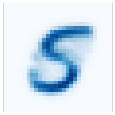
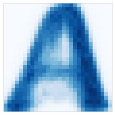
Mirror Prox for WB

Dual Extra-polation

IBP, $\gamma=10^{-3}$

IBP, $\gamma=10^{-5}$

Figure 1: WBs of hand-written digit ‘5’ (first row) and of letters ‘A’ (second row) computed by Algorithm 1 (Mirror Prox for WB), Algorithm 4 (Dual Extrapolation for WB) and the IBP with small values of the regularizing parameter.

MNIST and notMNIST.

In the paper, we mentioned that when a high-precision $\varepsilon$ of calculating Wasserstein barycenters is desired, the iterative Bregman projections (IBP) algorithm with regularizing parameter $\gamma$ is numerically unstable (as $\gamma$ must be selected proportional to $\varepsilon$ Peyré and Cuturi, (2018); Kroshnin et al., (2019)) in contrast to Algorithm 1 (Mirror Prox for WB) and Algorithm 4 (Dual Extrapolation for WB). Now we support this statement by computing Wasserstein barycenters of hand-written digits ‘5’ from the MNIST dataset and letters ‘A’ in a variety of fonts from the notMNIST dataset. Figure 1 illustrates the results obtained by the proposed algorithms in comparison with the IBP algorithm from the POT Python library with small values of regularizing parameter ($\gamma=10^{-3};10^{-5}$).

Gaussian measures.

To compare the convergence of the proposed algorithms, we randomly generated 10 Gaussian measures with equally spaced support of 100 points in $[-10,10]$, mean from $[-5,5]$ and variance from $[0.8,1.8]$. We studied the convergence of calculated barycenters to the theoretical true barycenter Delon and Desolneux, (2020). Figure 2 presents the convergence with respect to the function optimality gap $\frac{1}{m}\sum_{i=1}^{m}\mathcal{W}(p,q_{i})-\frac{1}{m}\sum_{i=1}^{m}\mathcal{W}(p^{*},q_{i})$. Here $p^{*}$ is the true barycenter. Despite the fact that Algorithm 4 has better complexity bound, Algorithm 1 has better convergence in practice. The slope ration $-1$ for the convergence of Algorithm 1 in log-scale perfectly fits the theoretical dependence of working time (iteration number $N$) on the desired accuracy $\varepsilon$ ($N\sim\varepsilon^{-1}$ from Theorem 3.3). For Algorithm 4, this slope ratio $-1$ is achieved only after a number of iterations but this is due to the need of solving practically computationally costly subproblems.

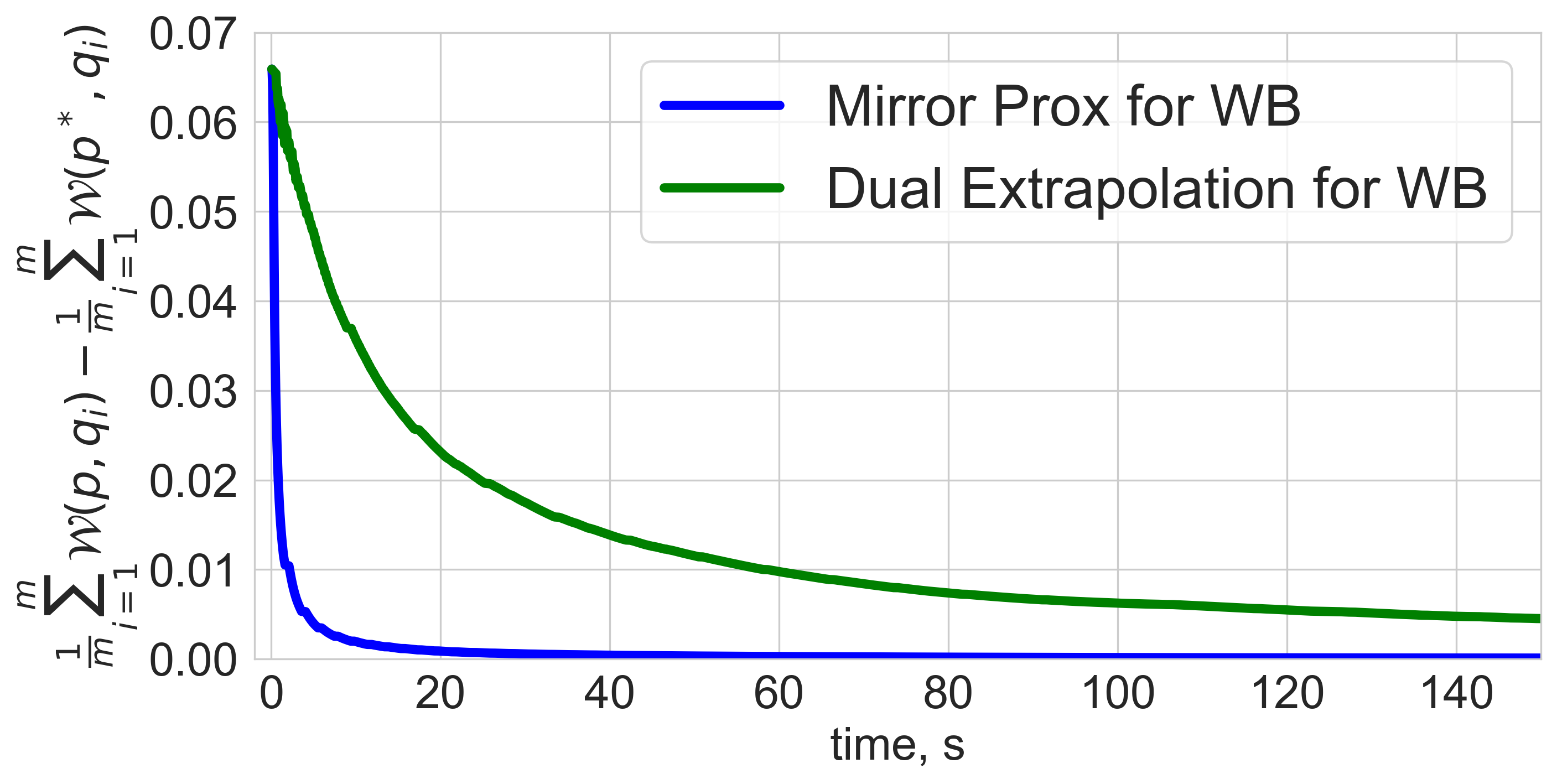
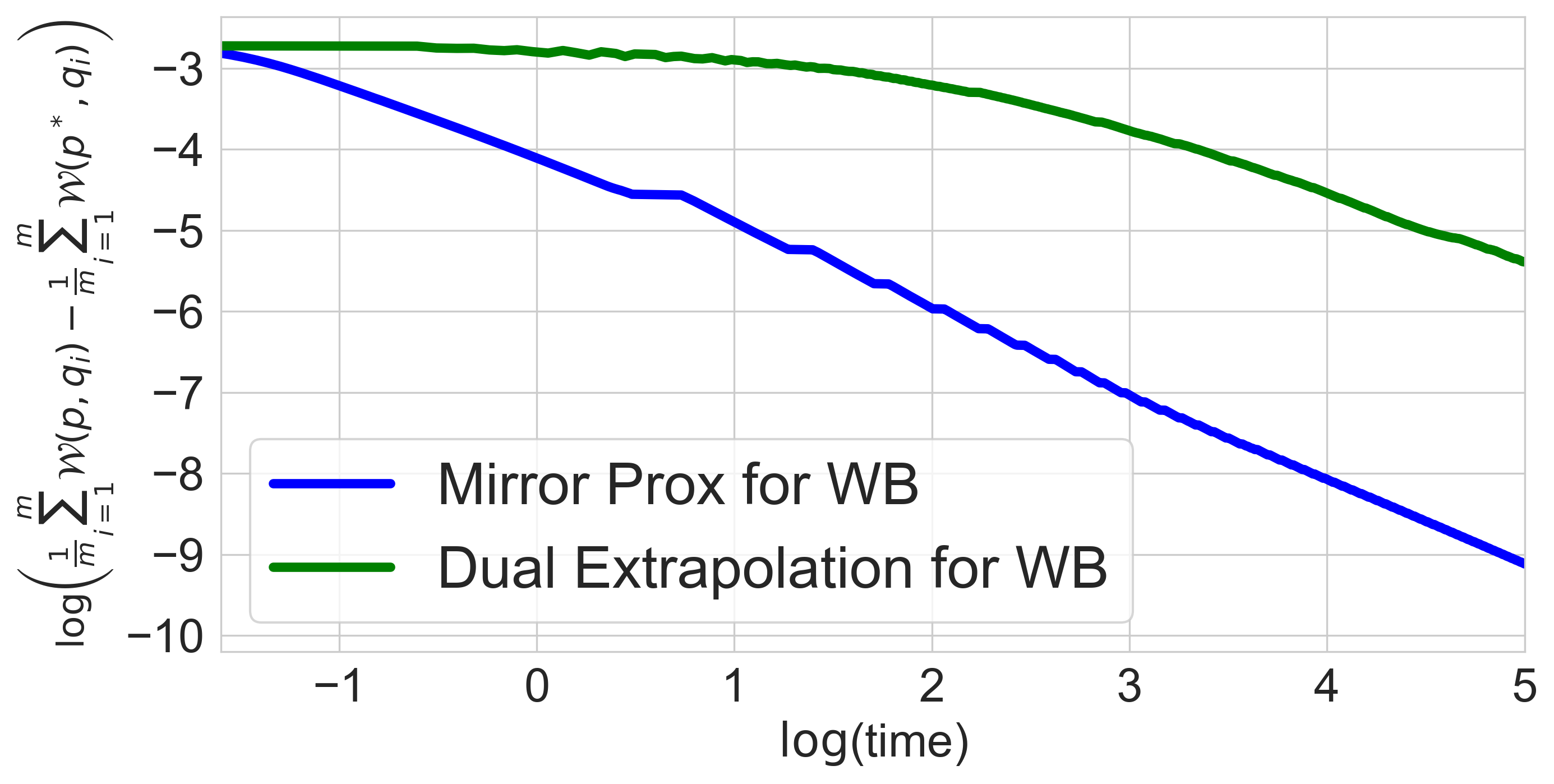
Figure 2: Convergence of Algorithm 1 (Mirror Prox for WB) and Algorithm 4 (Dual Extrapolation for WB) to the true barycenter of Gaussian measures w.r.t the function optimality gap $\frac{1}{m}\sum_{i=1}^{m}\mathcal{W}(p,q_{i})-\frac{1}{m}\sum_{i=1}^{m}\mathcal{W}(p^{*},q_{i})$. Here $p^{*}$ is the true barycenter.

Figure 3 illustrates the convergence of the barycenters obtained by Algorithms 1 and 4 to the true barycenter.

After 20 seconds

After 100 seconds

After 500 seconds

Figure 3: Convergence of the barycenters obtained by Algorithm 1 (Mirror Prox for WB) and Algorithm 4 (Dual Extrapolation for WB) to the true barycenter of Gaussian measures.

Next, we compare the convergence of the barycenters obtained by Algorithms 1 and 4 with the barycenter obtained by the IBP algorithm. Figure 4 demonstrates better approximations of the true Gaussian barycenter by Algorithms 1 and 4 compared to the $\gamma$-regularized IBP barycenter. The regularization parameter for the IBP algorithm (from the POT python library) is taken as smallest as possible under which the IBP still works since the smaller $\gamma$, the closer regularized IBP barycenter is to the true barycenter.

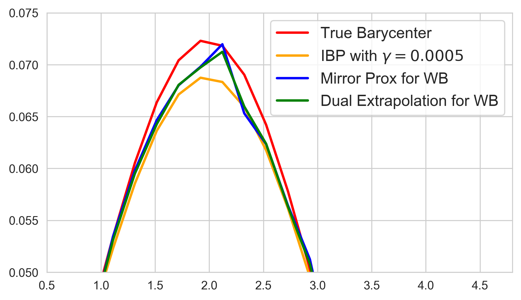
Figure 4: Convergence of the barycenters obtained by Algorithm 1 (Mirror Prox for WB), Algorithm 4 (Dual Extrapolation for WB), and the IBP to the true barycenter of Gaussian measures.

6 Conclusion

In this work, we provided two algorithms which have theoretical and practical interests. The main theoretical value is obtaining $\sqrt{n}$ faster algorithm for approximating Wasserstein barycenters of discrete measures with support $n$. The main practical value is the opportunity to calculate Wasserstein barycenters with a high desired precision that is not possible by using entropy-regularized based approaches.

Acknowledgements

The research of Section 3 is supported by the Ministry of Science and Higher Education of the Russian Federation (Goszadaniye) No. 075-00337-20-03, project No. 0714-2020-0005. The work of Section 4 was prepared within the framework of the HSE University Basic Research Program. The research of Section 5 is supported by the Russian Science Foundation (project 18-71-10108). The work of D. Tiapkin was fulfilled in Sirius, Sochi https://ssopt.org (August 2020), the work was initiated by A.Gasnikov.

7 MISSING PROOFS

7.1 Proof of Theorem 4.3

Theorem (Theorem 4.3).

$r$ is 3-area-convex with respect to the gradient operator $G$.

Proof.

Firstly, we define some notation connected to block-diagonal matrices. Assume that $D$ is a block diagonal matrix of size $ak\times bk$

$$D=\begin{pmatrix}B_{1}&0&\cdots&0\\ 0&B_{2}&\cdots&0\\ \vdots&\vdots&\ddots&\vdots\\ 0&0&\cdots&B_{k}\end{pmatrix},$$

where matrices $B_{i}$ of size $a\times b$. We refer to $i$-th block of $D$ as $D_{(i)}=B_{i}$. Also we define $D_{[i]}$ as a matrix $D$ with all blocks zeroes except the i-th one. Equivalent, we can write $D_{[i]}=\delta_{ii}^{(k)}\otimes D_{(i)}$, where $\delta_{ij}^{(k)}$ is a matrix of size $k\times k$ with $1$ on the position $i,j$ position and $0$ in any other, and $\otimes$ is a Kronecker product of matrices.

We will use a second-order criteria proposed by Jambulapati et al., (2019). We will show that

$$\begin{pmatrix}\nabla^{2}r(\mathbf{z})&-J\\ J&\nabla^{2}r(\mathbf{z})\end{pmatrix}\succeq 0,$$

where

$$J=\frac{2\|d\|_{\infty}}{m}\begin{pmatrix}0&\mathbf{A}^{T}\\ -\mathbf{A}&0\end{pmatrix}=\frac{2\|d\|_{\infty}}{n}\begin{pmatrix}0&0&\hat{A}^{\top}\\ 0&0&\mathcal{E}^{\top}\\ -\hat{A}&-\mathcal{E}&0\end{pmatrix}$$

is the Jacobian matrix for $F(\textbf{x},\textbf{y})$.

A good idea to remove a positive multiplicative term $2\|d\|_{\infty}m^{-1}$ to simplify the statement. Define $r^{\prime}(\mathbf{z})=1/(2\|d\|_{\infty}m^{-1})r(\mathbf{z})$ and $J^{\prime}=1/(2\|d\|_{\infty}m^{-1})J$. Hence we only should show that

$$P=\begin{pmatrix}\nabla^{2}r^{\prime}(\mathbf{z})&-J^{\prime}\\ J^{\prime}&\nabla^{2}r^{\prime}(\mathbf{z})\end{pmatrix}=\frac{m}{2\|d\|_{\infty}}\begin{pmatrix}\nabla^{2}r(\mathbf{z})&-J\\ J&\nabla^{2}r(\mathbf{z})\end{pmatrix}\succeq 0.$$

Then we can rewrite $r^{\prime}$ in the following manner

$$r^{\prime}(\mathbf{x},\mathbf{y}) =\sum_{i=1}^{m}\biggl{[}10\langle x_{i},\log x_{i}\rangle+\langle Ax_{i},(y_{i})^{2}\rangle\biggl{]}+5m\langle p,\log p\rangle-p^{T}\mathcal{E}^{T}(\mathbf{y}^{2})=$$

$$=\sum_{i=1}^{m}\biggl{[}10\langle x_{i},\log x_{i}\rangle+\langle Ax_{i},(y_{i})^{2}\rangle\biggl{]}+\sum_{i=1}^{m}\biggl{[}5\langle p,\log p\rangle+\langle B_{\mathcal{E}}p,(y_{i})^{2}\rangle\biggl{]}.$$

In this case, we can easily calculate the hessian of $r^{\prime}$, divide it into blocks:

$$\nabla^{2}r^{\prime}(\mathbf{z}) =\begin{pmatrix}\nabla^{2}_{\hat{x},\hat{x}}r^{\prime}(\mathbf{z})&\nabla^{2}_{\hat{x},p}r^{\prime}(\mathbf{z})&\nabla^{2}_{\hat{x},\mathbf{y}}r^{\prime}(\mathbf{z})\\ \nabla^{2}_{p,\hat{x}}r^{\prime}(\mathbf{z})&\nabla^{2}_{p,p}r^{\prime}(\mathbf{z})&\nabla^{2}_{p,\mathbf{y}}r^{\prime}(\mathbf{z})\\ \nabla^{2}_{\mathbf{y},\hat{x}}r^{\prime}(\mathbf{z})&\nabla^{2}_{\mathbf{y},p}r^{\prime}(\mathbf{z})&\nabla^{2}_{\mathbf{y},\mathbf{y}}r^{\prime}(\mathbf{z})\end{pmatrix}$$

$$=\begin{pmatrix}10\operatorname{diag}((\hat{x})^{-1})&0_{mn^{2}\times n}&2\hat{A}^{\top}\operatorname{diag}(\mathbf{y})\\ 0_{n\times mn^{2}}&5m\operatorname{diag}((p)^{-1})&-2\mathcal{E}^{\top}\operatorname{diag}(\mathbf{y})\\ 2\operatorname{diag}(\mathbf{y})\hat{A}&-2\operatorname{diag}(y)\mathcal{E}&2\operatorname{diag}(\hat{A}\hat{x})-2\operatorname{diag}(\mathcal{E}p)\end{pmatrix},$$

where $\operatorname{diag}(v)$ for a vector $v\in\mathbb{R}^{n}$ produces a diagonal matrix with $v$ on diagonal and $v^{-1}$ is a entry-wise operation on vector.

We notice that matrices $\operatorname{diag}((\hat{x})^{-1}),\hat{A}^{\top}\operatorname{diag}(\mathbf{y}),\operatorname{diag}(\hat{A}\hat{x})$ have a block-diagonal structure with $m$ blocks. Define the following matrices

$$B_{i}(\mathbf{z})=\begin{pmatrix}10\operatorname{diag}((\hat{x})^{-1})_{[i]}&0_{mn^{2}\times n}&2(\hat{A}^{\top}\operatorname{diag}(\mathbf{y}))_{[i]}\\ 0_{n\times mn^{2}}&0_{n\times n}&0_{n\times 2mn}\\ 2(\operatorname{diag}(\mathbf{y})\hat{A})_{[i]}&0_{2mn\times n}&2\operatorname{diag}(\hat{A}\hat{x})_{[i]}\end{pmatrix}$$

and

$$R(\mathbf{z})=\begin{pmatrix}0_{mn^{2}\times mn^{2}}&0_{mn^{2}\times n}&0_{mn^{2}\times 2mn}\\ 0_{n\times mn^{2}}&5m\operatorname{diag}((p)^{-1})&-2\mathcal{E}^{\top}\operatorname{diag}(\mathbf{y})\\ 0_{2mn\times mn^{2}}&-2\operatorname{diag}(y)\mathcal{E}&-2\operatorname{diag}(\mathcal{E}p)\end{pmatrix}.$$

Using these matrices, the decomposition of Hessian can be observed: $\nabla^{2}r^{\prime}(\mathbf{z})=\sum_{i=1}^{m}B_{i}(\mathbf{z})+R(\mathbf{z}).$

We notice that the matrix $J^{\prime}$ has the same block decomposition:

$$C_{i}=\begin{pmatrix}0&0&(\hat{A}^{\top})_{[i]}\\ 0&0&0\\ -(\hat{A})_{[i]}&0&0\end{pmatrix},\ \ \ S=\begin{pmatrix}0&0&0\\ 0&0&\mathcal{E}^{\top}\\ 0&-\mathcal{E}&0\end{pmatrix}.$$

Clearly we have $J^{\prime}=\sum_{i=1}^{m}C_{i}+S$. Using these two decompositions, we get the following:

$$P=\sum_{i=1}^{m}\underbrace{\begin{pmatrix}B_{i}(\mathbf{z})&-C_{i}\\ C_{i}&B_{i}(\mathbf{z})\end{pmatrix}}_{P_{i}}+\begin{pmatrix}R(\mathbf{z})&-S\\ S&R(\mathbf{z})\end{pmatrix}.$$

It can be observed that each matrix $P_{i}$ is almost a corresponding matrix for the area-convex regularizer for the optimal transportation problem with variables $x_{i},y_{i}$ in Jambulapati et al., (2019), except the rows and columns of zeros. Moreover, it was proven that these matrices are positive semi-definite. Hence, only the remaining term is need to be examined.

Firstly, we write the action of non-zero corner of $R(\mathbf{z})$, called $\hat{R}(\mathbf{z})$, as a quadratic form:

$$Q_{\hat{R}(\mathbf{z})}(u,v)=(u\top,v\top)\hat{R}(\mathbf{z})\begin{pmatrix}u\\ v\end{pmatrix}=(u\top,v\top)\begin{pmatrix}5m\operatorname{diag}((p)^{-1})&-2\mathcal{E}^{\top}\operatorname{diag}(\mathbf{y})\\ -2\operatorname{diag}(y)\mathcal{E}&-2\operatorname{diag}(\mathcal{E}p)\end{pmatrix}\begin{pmatrix}u\\ v\end{pmatrix}.$$

The we can use the trick induced by the structure of the matrix $\mathcal{E}$ to compute the quadratic form. The trick is about to rewrite $m$ in the following way: $m=\|\mathcal{E}_{:,j}\|_{1}=-\sum_{i=1}^{2mn}\mathcal{E}_{ij},\forall j\in[n].$

Then, we can calculate the quadratic form:

$$Q_{\hat{R}(\mathbf{z})}(u,v)=\sum_{i,j}(-\mathcal{E}_{ij})\left(\frac{5u_{j}^{2}}{p_{j}}+4u_{j}v_{i}y_{i}+2v_{i}^{2}p_{j}\right).$$

Secondly, we wrtie the action of non-zero corner of $S$, called $\hat{S}$, as a bilinear form

$$B_{\hat{S}}((a,b),(u,v))=(x\top,y\top)\begin{pmatrix}0&\mathcal{E}^{\top}\\ -\mathcal{E}&0\end{pmatrix}\begin{pmatrix}u\\ v\end{pmatrix}=\sum_{i,j}\mathcal{E}_{ij}\left(a_{j}v_{i}-u_{j}b_{i}\right),$$

and, as a result, we have the complete analytic expression for the quadratic form induced by the remaining term of $P$:

$$((a^{\top},b^{\top}),(u^{\top},v^{\top})) \begin{pmatrix}\hat{R}(\mathbf{z})&-\hat{S}\\ \hat{S}&\hat{R}(\mathbf{z})\end{pmatrix}\begin{pmatrix}\left(\begin{array}[]{c}a\\ b\end{array}\right)\\ \left(\begin{array}[]{c}u\\ v\end{array}\right)\end{pmatrix}$$

$$=\sum_{i,j}(-\mathcal{E}_{ij})\left(\frac{5a_{j}^{2}}{p_{j}}+4a_{j}b_{i}y_{i}+2b_{i}^{2}p_{j}+2a_{j}v_{i}-2u_{j}b_{i}+\frac{5u_{j}^{2}}{p_{j}}+4u_{j}v_{i}y_{i}+2v_{i}^{2}p_{j}\right)$$

$$=\sum_{i,j}(-\mathcal{E}_{ij})\frac{1}{p_{j}}\biggl{(}(2a_{j}y_{i}+b_{i}p_{j})^{2}+(2u_{j}y_{i}+v_{i}p_{j})^{2}$$

$$+(a_{j}+v_{i}p_{j})^{2}+(u_{j}+b_{i}p_{j})^{2}+(1-(y_{i})^{2})(a_{j}^{2}+u_{j}^{2}))\biggl{)}\geq 0.$$

The final inequality follows from the range of $y_{i}\in[-1,1]$ and finishes the proof. ∎

7.2 Proof of Theorem 4.4

Theorem (Theorem 4.4).

Let at each iteration, Dual Extrapolation algorithm calls Alternating minimization (AM) scheme to make the proximal steps. Then for $N=\lceil\frac{4\kappa\Theta}{\varepsilon}\rceil$ iterations of Dual Extrapolation algorithm running with regularizer (18) and $\kappa=3$, AM scheme accumulates additive error $\varepsilon/2$ running with

$$M=24\log\left(\left(\frac{88\|d\|_{\infty}}{\varepsilon^{2}}+\frac{4}{\varepsilon}\right)\Theta+\frac{36\|d\|_{\infty}}{\varepsilon}\right)$$

iterations in $O(mn^{2}\log\gamma)$ time, where $\gamma=\varepsilon^{-1}\|d\|_{\infty}\log n$.

To prove this theorem we will use the results from Jambulapati et al., (2019) about their Alternating minimization scheme. Firstly, we need to obtain a linear convergence and we can do it by adapting an argument of Jambulapati et al., (2019, Lemma 6) to our setup.

Lemma 7.1.

For some $\mathbf{x}^{k+1},\mathbf{y}_{k}$, let $\mathcal{X}_{k+1}=\{\mathbf{x}\mid\mathbf{x}\geq\frac{1}{2}\mathbf{x}^{k+1}\}$ where inequality is entrywise, and let $\mathcal{Y}_{k}$ be the entire domain of $\mathbf{y}$ (i.e. $\mathcal{Y}$). Then for any $\mathbf{x}^{\prime}\in\mathcal{X}_{k+1},\mathbf{y}^{\prime},\mathbf{y}^{\prime\prime}\in\mathcal{Y}_{k}$,

$$\nabla^{2}r(\mathbf{x}^{\prime},\mathbf{y}^{\prime})\succeq\frac{1}{12}\nabla^{2}_{\mathbf{y}\mathbf{y}}r(\mathbf{x}^{k+1},\mathbf{y}^{\prime\prime}).$$

Proof.

The only thing that differs in the analysis is a diagonal approximation then does not depends on $\mathbf{y}$. Hence, we only need to show that for any $\mathbf{y}$

$$D(\mathbf{x})\preceq\nabla^{2}r(\mathbf{x},\mathbf{y})\preceq 6D(\mathbf{x}),$$

where $D(\mathbf{x})$ is the diagonal approximation

$$D(\mathbf{x})=\begin{pmatrix}2\operatorname{diag}((\hat{x})^{-1})&0_{mn^{2}\times n}&0_{mn^{2}\times 2mn}\\ 0_{n\times mn^{2}}&m\operatorname{diag}((p)^{-1})&0_{n\times 2mn}\\ 0_{2mn\times mn^{2}}&0_{2mn\times n}&\operatorname{diag}(\hat{A}\hat{x})-\operatorname{diag}(\mathcal{E}p)\end{pmatrix}.$$

It is easy to see that $D(\mathbf{x})$ has the same block structure as $\nabla^{2}r(\mathbf{x},\mathbf{y})$ and we can prove our inequalities for each block separately. But all blocks connected to $\hat{x}$ is blocks that appears in optimal transport problem and the required inequalities were proven in Jambulapati et al., (2019). Hence, we only need to show that

$$\hat{D}_{p}(\mathbf{x})\preceq\hat{R}(\mathbf{x},\mathbf{y})\preceq 6\hat{D}_{p}(\mathbf{x}),$$

where

$$\hat{D}_{p}(\mathbf{x})=\begin{pmatrix}m\operatorname{diag}((p)^{-1})&0_{n\times 2mn}\\ 0_{2mn\times n}&-\operatorname{diag}(\mathcal{E}p)\end{pmatrix}.$$

and $\hat{R}$ was defined in the proof of Theorem 4.3.

Also, in the proof of Theorem 4.3 we show that

$$Q_{\hat{R}(\mathbf{z})}(u,v)=\sum_{i,j}(-\mathcal{E}_{ij})\left(\frac{5u_{j}^{2}}{p_{j}}+4u_{j}v_{i}y_{i}+2v_{i}^{2}p_{j}\right).$$

Using the same idea, we can write the action of quadratic form induced by $\hat{D}_{p}$:

$$Q_{\hat{D}_{p}(\mathbf{x})}(u,v)=\sum_{i,j}(-\mathcal{E}_{ij})\left(\frac{u_{j}^{2}}{p_{j}}+v_{i}^{2}p_{j}\right).$$

Using the fact that $y_{i}\in[-1,1]$, we can obtain the required by the following inequalities and finish the proof:

$$\frac{u_{j}^{2}}{p_{j}}+v_{i}^{2}p_{j}\leq\frac{5u_{j}^{2}}{p_{j}}+4u_{j}v_{i}y_{i}+2v_{i}^{2}p_{j}\leq\frac{6u_{j}^{2}}{p_{j}}+6v_{i}^{2}p_{j}.$$

∎

By the exactly same arguments, we obtain the linear rate of converge for our Alternating Minimization (AM) scheme. We need to show last two points

• Bound the complexity of each iteration

• Bound the initial range

Lemma 7.2.

For $H(\mathbf{x},\mathbf{y})$, defined in (19), we can implement the steps

1. $\mathbf{x}^{k+1}\triangleq\arg\min\limits_{\mathbf{x}\in\mathcal{X}}H(\mathbf{x},\mathbf{y}^{k})$,

2. $\mathbf{y}^{k+1}\triangleq\arg\min\limits_{\mathbf{y}\in\mathcal{Y}}H(\mathbf{x}^{k+1},\mathbf{y})$,

in time $O(mn^{2})$.

Proof.

First of all, divide a vector $\bm{v}$ from the definition of function (19) into $m+1$ part and vector $\bm{u}$ into $m$ parts. We have the following function to optimize by some regrouping and rewriting a regularizer in homogeneous manner

$$H(\mathbf{x},\mathbf{y}) =\frac{2\|d\|_{\infty}}{m}\sum_{i=1}^{m}\biggl{(}\frac{m}{2\|d\|_{\infty}}\langle v_{i},x_{i}\rangle+\langle(y_{i})^{2},Ax_{i}\rangle+10\langle x_{i},\log x_{i}\rangle$$

$$+\frac{m}{2\|d\|_{\infty}}\langle u_{i},y_{i}\rangle+\langle B_{\mathcal{E}}p,(y_{i})^{2}\rangle\biggl{)}+10\|d\|_{\infty}\langle p,\log p\rangle+\langle v_{m+1},p\rangle.$$

We notice that each $x_{i}$ is independent from others and we can compute $x^{(k+1)}_{i}$ apart as a solutions of the following optimization problems:

$$x^{k+1}_{i}=\arg\min_{x\in\Delta^{n^{2}}}\left\langle\underbrace{\frac{m}{20\|d\|_{\infty}}v_{i}+\frac{1}{10}A^{\top}(y_{i}^{k})^{2}}_{\gamma_{i}},x\right\rangle+\langle x,\log x\rangle,$$

and the solution of this type of problems is well-known and proportional to $\exp(-\gamma_{i})$. The multiplication on the matrix $A$ and $A^{\top}$ can be computed in $O(n^{2})$ time, because these matrices consists of $O(n^{2})$ non-zero entries, and all these steps can be performed in $O(mn^{2})$.

Also we need to compute an optimal $p$ by the same idea

$$p^{k+1}=\arg\min_{p\in\Delta^{n}}\left\langle\underbrace{\frac{1}{10\|d\|_{\infty}}v_{m+1}-\frac{1}{5m}\mathcal{E}^{\top}(\mathbf{y}^{k})^{2}}_{\gamma_{m+1}},p\right\rangle+\langle p,\log p\rangle.$$

As in the previous case, an optimal $p^{k+1}$ is proportional to $\exp(-\gamma_{m+1})$ and it can be computed in $O(mn^{2})$ time.

For the computation of $\mathbf{y}^{(k+1)}$ we notice that each $[y^{(k+1)}_{i}]_{j}$ can be computed separately as a solution of the following 1-D optimization problem:

$$[y^{k+1}_{i}]_{j}=\arg\min_{y\in[-1,1]}\frac{m}{2\|d\|_{\infty}}[u_{i}]_{j}\cdot y+([Ax_{i}^{k+1}]_{j}+[B_{\mathcal{E}}p^{k+1}]_{j})\cdot y^{2}.$$

It could be easily solved in constant time if we know $Ax_{i}^{k+1}$ and $B_{\mathcal{E}}p^{k+1}=(p^{\top},0_{n})^{\top}$

$$[y^{k+1}_{i}]_{j}=\begin{cases}-1,&\alpha\leq-1\\ 1,&\alpha\geq 1\\ \alpha,&\alpha\in[-1,1]\end{cases},\quad\text{where }\alpha=\frac{-m[u_{i}]_{j}}{4\|d\|_{\infty}([Ax_{i}]_{j}+[B_{\mathcal{E}}p]_{j})}.$$

Hence, we can make all calculations in $O(mn^{2})$. ∎

Now we are ready to write the final proof.

Proof of Theorem 4.4..

To proof the final result, we need to remind the proximal operator for $r$:

$$\operatorname{prox}_{\bar{\mathbf{z}}}^{r}(v)=\arg\min_{\mathbf{z}\in\mathcal{Z}}\langle v,\mathbf{z}\rangle+B_{r}(\bar{z},\mathbf{z})=\arg\min_{\mathbf{z}\in\mathcal{Z}}\langle v-\nabla r(\bar{\mathbf{z}}),\mathbf{z}\rangle+r(\mathbf{z}).$$

We notice, that it is equivalent to the next view, separate over $\mathbf{x}$ and $\mathbf{y}$:

$$\operatorname{prox}_{\bar{\mathbf{x}},\bar{\mathbf{y}}}^{r}(v)=\arg\min_{\mathbf{x}\in\mathcal{X},\mathbf{y}\in\mathcal{Y}}\langle v_{x}-\nabla_{\mathbf{x}}r(\bar{\mathbf{x}},\bar{\mathbf{y}}),\mathbf{x}\rangle+\langle v_{y}-\nabla_{\mathbf{y}}r(\bar{\mathbf{x}},\bar{\mathbf{y}}),\mathbf{y}\rangle+r(\mathbf{x},\mathbf{y}).$$ (20)

We have precisely the type of problems that can be solved using AM scheme described above in linear time, moreover, each step reduces error by $1/24$ factor (similar as Jambulapati et al., (2019)).

The only thing we need to bound is an initial error. For this goal we should bound the norm of the gradient and the argument of the proximal function in all calls during the algorithm.

Firstly, divide gradient operator $G(\mathbf{z})=(G_{\mathbf{x}}(\mathbf{z})^{\top},G_{\mathbf{y}}(\mathbf{z})^{\top})^{\top}$, defined in (7), into two parts and bound uniformly $\ell_{\infty}$ and $\ell_{1}$ norms of each part respectively

$$\|G_{\mathbf{x}}(\mathbf{z})\|_{\infty} =\frac{1}{m}\|\bm{d}+2\|d\|_{\infty}\bm{A}^{\top}\mathbf{y}\|_{\infty}\leq\frac{\|d\|_{\infty}}{m}+\frac{2\|d\|_{\infty}}{m}\|\bm{A}^{\top}\mathbf{y}\|_{\infty}\leq 3\|d\|_{\infty},$$

$$\|G_{\mathbf{x}}(\mathbf{z})\|_{1}\ =\frac{1}{m}\|2\|d\|_{\infty}(\bm{c}-\bm{A}\mathbf{x})\|_{1}\leq\frac{2\|d\|_{\infty}}{m}\left(\|\bm{c}\|_{1}+\|\bm{A}\mathbf{x}\|_{1}\right)\leq 8\|d\|_{\infty}.$$

In the inequality in the first row we used the fact $m\geq 1$ for simplicity and in the second one we use the fact that matrix $A$ and vector $x_{i}$ are non-negative, hence, $\|Ax_{i}\|_{1}=\langle\mathbf{1}_{n},Ax_{i}\rangle=2\langle\mathbf{1}_{n},x_{i}\rangle=2$, where $\mathbf{1}_{n}$ is a vector consists of ones.

Then we can use the fact that the argument of the first prox-operator $\mathbf{s}^{k}=(\mathbf{s}^{k}_{\mathbf{x}},\mathbf{s}^{k}_{\mathbf{y}})$ is a sum of $k$ gradients multiplied by $1/2\kappa$, computed in different points. In the second operator we also add gradient operator, multiplied by $1/\kappa$. Since $k\leq{4\kappa\Theta\cdot\varepsilon^{-1}}$, we have by triangle inequality

$$\|\mathbf{s}^{k}_{\mathbf{x}}\|_{\infty} \leq\frac{k}{2\kappa}\cdot 3\|d\|_{\infty}\leq\frac{6\Theta\|d\|_{\infty}}{\varepsilon},$$

$$\|\mathbf{s}^{k}_{\mathbf{y}}\|_{1}\ \leq\frac{k}{2\kappa}8\|d\|_{\infty}\leq\frac{16\Theta\|d\|_{\infty}}{\varepsilon}.$$

Then, all our arguments of the proximal operator during the running time can be bounded in the following way (for $\kappa=3$)

$$\|v_{\mathbf{x}}\|_{\infty} \leq\frac{6\Theta\|d\|_{\infty}}{\varepsilon}+\|d\|_{\infty},$$

$$\|v_{\mathbf{y}}\|_{1}\ \leq\frac{16\Theta\|d\|_{\infty}}{\varepsilon}+\frac{8}{3}\|d\|_{\infty}.$$

Then fix $\mathbf{x}^{*}$ and $\mathbf{y}^{*}$ as minimizers for the proximal operator (20) and remind the bound for $\Theta\leq 40\log n\|d\|_{\infty}+6\|d\|_{\infty}$. Also we can compute $\|\nabla_{\mathbf{x}}r(\bar{\mathbf{x}},\bar{\mathbf{y}})\|_{\infty}\leq 20\|d\|_{\infty}(2\log n+1)$ and $\|\nabla_{\mathbf{y}}r(\bar{x},\bar{y})\|_{1}=0$.

Then we can write a suboptimality gap $\delta_{0}$ for our algorithm for any initial $\mathbf{x}^{0}$ and $\mathbf{y}^{0}$:

$$\delta_{0} =\langle v_{\mathbf{x}}-\nabla_{\mathbf{x}}r(\bar{\mathbf{x}},\bar{\mathbf{y}}),\mathbf{x}^{0}-\mathbf{x}^{*}\rangle+\langle v_{\mathbf{y}}-\nabla_{\mathbf{y}}r(\bar{\mathbf{x}},\bar{\mathbf{y}}),\mathbf{y}^{0}-\mathbf{y}^{*}\rangle+r(\mathbf{x}^{0},\mathbf{y}^{0})-r(\mathbf{x}^{*},\mathbf{y}^{*})$$

$$\leq\|v_{\mathbf{x}}-\nabla_{\mathbf{x}}r(\bar{\mathbf{x}},\bar{\mathbf{y}})\|_{\infty}\|\mathbf{x}^{0}-\mathbf{x}^{*}\|_{1}+\|v_{\mathbf{y}}-\nabla_{\mathbf{y}}r(\bar{\mathbf{x}},\bar{\mathbf{y}})\|_{1}\|\mathbf{y}^{0}-\mathbf{y}^{*}\|_{\infty}+\Theta$$

$$\leq 2\|d\|_{\infty}\cdot\left(\frac{6\Theta}{\varepsilon}+20\log n+10\right)+\|d\|_{\infty}+2\cdot\frac{16\Theta\|d\|_{\infty}}{\varepsilon}+\frac{8}{3}\|d\|_{\infty}+\Theta$$

$$\leq\left(\frac{44\|d\|_{\infty}}{\varepsilon}+2\right)\Theta+18\|d\|_{\infty}.$$

Then we can compute the total number of iterations to obtain $\varepsilon/2$ desired accuracy:

$$N=\log_{24/23}\frac{2\delta_{0}}{\varepsilon}\leq 24\log\left(\left(\frac{88\|d\|_{\infty}}{\varepsilon^{2}}+\frac{4}{\varepsilon}\right)\Theta+\frac{36\|d\|_{\infty}}{\varepsilon}\right)=O(\log\gamma),$$

where $\gamma=\|d\|\varepsilon^{-1}\log n$, as desired. Each iteration can be done in $O(mn^{2})$ time and we obtain the required complexity. ∎

References

- Allen-Zhu et al., (2017) Allen-Zhu, Z., Li, Y., Oliveira, R., and Wigderson, A. (2017). Much faster algorithms for matrix scaling. In 2017 IEEE 58th Annual Symposium on Foundations of Computer Science (FOCS), pages 890–901. https://arxiv.org/abs/1704.02315.
- Arjovsky et al., (2017) Arjovsky, M., Chintala, S., and Bottou, L. (2017). Wasserstein GAN. arXiv:1701.07875.
- Benamou et al., (2015) Benamou, J.-D., Carlier, G., Cuturi, M., Nenna, L., and Peyré, G. (2015). Iterative bregman projections for regularized transportation problems. SIAM Journal on Scientific Computing, 37(2):A1111–A1138.
- Bigot et al., (2012) Bigot, J., Klein, T., et al. (2012). Consistent estimation of a population barycenter in the wasserstein space. ArXiv e-prints.
- Blanchet et al., (2018) Blanchet, J., Jambulapati, A., Kent, C., and Sidford, A. (2018). Towards optimal running times for optimal transport. arXiv preprint arXiv:1810.07717.
- Bubeck, (2014) Bubeck, S. (2014). Theory of convex optimization for machine learning. arXiv preprint arXiv:1405.4980, 15.
- Cohen et al., (2017) Cohen, M. B., Madry, A., Tsipras, D., and Vladu, A. (2017). Matrix scaling and balancing via box constrained newton’s method and interior point methods. In 2017 IEEE 58th Annual Symposium on Foundations of Computer Science (FOCS), pages 902–913. https://arxiv.org/abs/1704.02310.
- Cuturi, (2013) Cuturi, M. (2013). Sinkhorn distances: Lightspeed computation of optimal transport. In Advances in Neural Information Processing Systems, pages 2292–2300.
- Delon and Desolneux, (2020) Delon, J. and Desolneux, A. (2020). A wasserstein-type distance in the space of gaussian mixture models. SIAM Journal on Imaging Sciences, 13(2):936–970.
- Dvurechensky et al., (2018) Dvurechensky, P., Gasnikov, A., and Kroshnin, A. (2018). Computational optimal transport: Complexity by accelerated gradient descent is better than by Sinkhorn’s algorithm. In Dy, J. and Krause, A., editors, Proceedings of the 35th International Conference on Machine Learning, volume 80, pages 1367–1376. arXiv:1802.04367.
- Ebert et al., (2017) Ebert, J., Spokoiny, V., and Suvorikova, A. (2017). Construction of non-asymptotic confidence sets in 2-Wasserstein space. arXiv:1703.03658.
- Guminov et al., (2019) Guminov, S., Dvurechensky, P., and Gasnikov, A. (2019). Accelerated alternating minimization. arXiv preprint arXiv:1906.03622.
- Jambulapati et al., (2019) Jambulapati, A., Sidford, A., and Tian, K. (2019). A direct iteration parallel algorithm for optimal transport. In Advances in Neural Information Processing Systems, pages 11359–11370.
- Kroshnin et al., (2019) Kroshnin, A., Tupitsa, N., Dvinskikh, D., Dvurechensky, P., Gasnikov, A., and Uribe, C. (2019). On the complexity of approximating Wasserstein barycenters. In Chaudhuri, K. and Salakhutdinov, R., editors, Proceedings of the 36th International Conference on Machine Learning, volume 97, pages 3530–3540. arXiv:1901.08686.
- Lin et al., (2020) Lin, T., Ho, N., Chen, X., Cuturi, M., and Jordan, M. I. (2020). Fixed-support wasserstein barycenters: Computational hardness and fast algorithm.
- Nemirovski, (2004) Nemirovski, A. (2004). Prox-method with rate of convergence o (1/t) for variational inequalities with lipschitz continuous monotone operators and smooth convex-concave saddle point problems. SIAM Journal on Optimization, 15(1):229–251.
- Nesterov, (2007) Nesterov, Y. (2007). Dual extrapolation and its applications to solving variational inequalities and related problems. Mathematical Programming, 109(2-3):319–344.
- Peyré and Cuturi, (2018) Peyré, G. and Cuturi, M. (2018). Computational optimal transport. arXiv:1803.00567.
- Rachev et al., (2011) Rachev, S. T., Stoyanov, S. V., and Fabozzi, F. J. (2011). A probability metrics approach to financial risk measures. John Wiley & Sons.
- Sherman, (2017) Sherman, J. (2017). Area-convexity, regularization, and undirected multicommodity flow. In Proceedings of the 49th Annual ACM SIGACT Symposium on Theory of Computing, pages 452–460.
- Solomon et al., (2015) Solomon, J., De Goes, F., Peyré, G., Cuturi, M., Butscher, A., Nguyen, A., Du, T., and Guibas, L. (2015). Convolutional wasserstein distances: Efficient optimal transportation on geometric domains. ACM Transactions on Graphics (TOG), 34(4):66.
- Tarjan, (1997) Tarjan, R. E. (1997). Dynamic trees as search trees via euler tours, applied to the network simplex algorithm. Mathematical Programming, 78(2):169–177.