BCS-BEC Crossover Effects and Pseudogap in Neutron Matter

Abstract

Due to the large neutron-neutron scattering length, dilute neutron matter resembles the unitary Fermi gas, which lies half-way in the crossover from the BCS phase of weakly coupled Cooper pairs to the Bose-Einstein condensate of dimers. We discuss crossover effects in analogy with the T-matrix theory used in the physics of ultracold atoms, which we generalize to the case of a non-separable finite-range interaction. A problem of the standard Nozières–Schmitt-Rink approach and different ways to solve it are discussed. It is shown that in the strong-coupling regime, the spectral function exhibits a pseudo-gap at temperatures above the critical temperature $T_{c}$. The effect of the correlated density on the density dependence of $T_{c}$ is found to be rather weak, but a possibly important effect due to the reduced quasiparticle weight is identified.

I Introduction

The inner crust of neutron stars is characterized by the presence of a dilute gas of neutrons in between much denser clusters Chamel and Haensel (2008). The superfluidity of this gas is of decisive importance, e.g., to explain pulsar glitches and to determine the thermal evolution of neutron stars. Nevertheless, in spite of a long effort and the existence of Quantum Monte-Carlo (QMC) calculations of the gap at low densities Abe and Seki (2009); Gezerlis and Carlson (2010), there remain large uncertainties about the density dependence of the pairing gap and the critical temperature of neutron matter.

In reality, the neutron gas in the inner crust is not uniform because of the nuclear clusters. However, if the pairing is strong enough and the Cooper-pair size (coherence length) small enough, i.e., much smaller than the distance between clusters, it should be possible to treat the neutron gas approximately as uniform matter, except near the cluster surface Okihashi and Matsuo (2020). Furthermore, in the cases where the local-density approximation is not valid, the calculations rely generally on density-dependent effective interactions, fitted such that they reproduce, at the mean-field level, the realistic pairing gaps in uniform matter Chamel et al. (2010); Okihashi and Matsuo (2020). So, also in this case, the understanding of uniform neutron matter is a necessary prerequisite to describe superfluidity of the inner crust.

The neutron-neutron ($nn$) interaction has a very large scattering length $a\simeq-18.7\pm 0.6\;\text{fm}$ González Trotter et al. (1999) or $-16.59\pm 1.17\;\text{fm}$ Babenko and Petrov (2013)) while its effective range is only $r_{0}=2.83\pm 0.11\;\text{fm}$ Babenko and Petrov (2013). Hence, at low densities, when the mean distance between the neutrons is between $3$ and $16\;\text{fm}$, the neutron gas resembles a unitary Fermi gas, an idealized system of spin-$1/2$ Fermions with a contact interaction having infinite scattering length, which was originally introduced as a schematic model of dilute neutron matter Baker (1999).

A few years later, the unitary Fermi gas was experimentally realized with ultracold trapped gases of alkali atoms, where the interaction has practically zero range (four orders of magnitude smaller than the interparticle distance) and the scattering length can be tuned with the help of a magnetic field from negative to positive values by passing through infinity at the so-called Feshbach resonance. This allows one to study not only the unitary limit, but the whole crossover from BCS pairing with Cooper pairs in the case of weakly attractive interactions ($a<0$) to the Bose-Einstein condensation (BEC) of bound dimers in the case $a>0$ Calvanese Strinati et al. (2018). The unitary limit is just a special case in this crossover, corresponding to the situation where the binding energy of the dimer in free space tends to zero.

On the BEC side and in the crossover region, it is crucial for a correct description of the superfluid phase transition that pair correlations persist at temperatures above the critical temperature $T_{c}$. On the BEC side of the crossover, these correlations can easily be interpreted as dimers which are already formed but not yet condensed. This implies in particular that the BCS relation $T_{c}=0.57\,\Delta(0)$ between the critical temperature $T_{c}$ and the zero-temperature pairing gap $\Delta(0)$ is not fulfilled in this regime. The simplest theory that correctly interpolates between the BCS and the BEC limits was proposed by Nozières and Schmitt-Rink (NSR) Nozières and Schmitt-Rink (1985).

In nuclear systems, the interaction is of course fixed. Nevertheless, a BCS-BEC crossover is expected to happen in symmetric nuclear matter if one varies the density: at very low density, there will be a BEC of deuterons, which continuously goes over to a BCS superfluid with proton-neutron Cooper pairs at higher density Baldo et al. (1995). The critical temperature $T_{c}$ in this crossover was studied in Schmidt et al. (1990); Stein et al. (1995); Jin et al. (2010) using an approach similar to the NSR theory.

The case of neutron matter is somewhat different, because no bound dineutron state and hence no BEC phase exist. Nevertheless, with varying density, neutron matter passes from the strongly coupled regime close to the unitary limit to the weakly coupled BCS regime. The relevance of BCS-BEC crossover-like physics in dilute neutron matter was pointed out in Matsuo (2006). Consequently, NSR-like corrections of $T_{c}$ due to pair correlations in the normal phase were studied in Ramanan and Urban (2013, 2018); Tajima et al. (2019); Urban and Ramanan (2020), and in Ohashi et al. (2020); Inotani et al. (2019) the NSR-like approach was also extended to temperatures below $T_{c}$.

In previous work following the NSR and related approaches, the single-particle self-energy and spectral function were usually not computed. One reason is that in these approaches the density $\rho$ is often obtained as the derivative of the thermodynamic potential with respect to the chemical potential $\mu$ Nozières and Schmitt-Rink (1985); Sá de Melo et al. (1993); Tajima et al. (2019); Ohashi et al. (2020); Inotani et al. (2019). Computing the thermodynamic potential in the ladder approximation, one automatically obtains an expression which is equivalent to truncating the Dyson equation for the single-particle Green’s function at the first order in the self-energy Calvanese Strinati et al. (2018). In this case, when calculating only the density $\rho$ and not the occupation numbers $n(k)$, the somewhat difficult computation of the self-energy can be avoided. However, some problems of the different approaches show up when one looks at the occupation numbers $n(k)$, and some interesting aspects of the crossover regime, such as the existence of a pseudogap, can only be studied by looking at the spectral function. In this context, let us note that the density of states, which is usually considered when discussing the pseudogap, is obtained by integrating the spectral function over momentum.

In the present work, we revisit this problem, but now we compute the self-energy, which gives us access to the occupation numbers and to the spectral function. In Sec. II, we recall the T matrix formalism and discuss in some detail the way we deal with non-separable interactions. In Sec. III, we will show our results for the spectral function, the pseudogap, the correlated occupation numbers, and the density dependence of the critical temperature. We will in particular discuss the differences between the original NSR approach, its modifications that have been used previously, and our more complete treatment of the self-energy. Some open questions are discussed in Sec. IV, and we conclude in Sec. V.

II T-matrix formalism

II.1 Vertex function

The superfluid phase transition is an instability of the normal phase towards the superfluid one which shows up in the two-particle T matrix (vertex function) $\Gamma$. We compute $\Gamma$ within the ladder approximation, i.e., by resumming ladder diagrams in the medium. In this formalism, the vertex function for total momentum $k$, in- and outgoing relative momenta $q$ and $q^{\prime}$, and total energy of the pair $\omega$, is the solution of the following Lippmann-Schwinger like equation corresponding to the Feynman diagrams shown in Fig. 1(a),

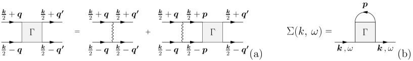
Figure 1: Feynman diagrams for (a) the vertex function $\Gamma$ and (b) the self-energy $\Sigma$ in ladder approximation.

$$\Gamma(q,q^{\prime},k,\omega)=v(q,q^{\prime})+\int\dfrac{d^{3}\mathbf{p}}{(2\pi)^{3}}\,v(q,p)\,G_{0}^{(2)}(\mathbf{p},\textbf{\text{k}},\omega)\,\Gamma(p,q^{\prime},k,\omega)\,,$$ (1)

where $v(q,q^{\prime})$ is the matrix element of the $s$-wave $nn$ interaction. In our calculations, we will use interactions of the $V_{\text{low-}k}$ type Bogner et al. (2010). Notice that, in contrast to nuclear matter with protons or very dense neutron matter Holt et al. (2010), the effect of three-body interactions is not important in dilute neutron matter because the leading contact term is forbidden by the Pauli principle.

At finite temperature, the two-particle Green’s function $G_{0}^{(2)}$ is written within the Matsubara formalism Fetter and Walecka (1971) as

$$G_{0}^{(2)}(\mathbf{p},\textbf{\text{k}},i\Omega_{N})=\dfrac{1}{\beta}\sum_{n}G_{0}(|\tfrac{\textbf{\text{k}}}{2}+\mathbf{p}|,i\omega_{n})\,G_{0}(|\tfrac{\textbf{\text{k}}}{2}-\mathbf{p}|,i\Omega_{N}-i\omega_{n})\,,$$ (2)

where $\xi_{k}=\hbar^{2}k^{2}/(2m)-\mu$ is the neutron single-particle energy relative to the chemical potential $\mu$, with $\hbar$ the reduced Planck constant and $m$ the neutron mass, $\beta=1/T$ is the inverse of the temperature $T$, $\Omega_{N}=2\pi NT$ and $\omega_{n}=(2n+1)\pi T$ are bosonic and fermionic Matsubara frequencies, respectively, and $G_{0}(k,i\omega_{n})=1/(i\omega_{n}-\xi_{k})$ is the free single-particle Green’s function. After summation over $\omega_{n}$ and analytic continuation to the real $\omega$ axis, we obtain the retarded two-particle Green’s function

$$G_{0}^{(2)}(\mathbf{p},\textbf{\text{k}},\omega)=\dfrac{1-f_{\text{\tiny{F}}}(\xi_{\textbf{\text{k}}/2+\mathbf{p}})-f_{\text{\tiny{F}}}(\xi_{\textbf{\text{k}}/2-\mathbf{p}})}{\omega-\xi_{\textbf{\text{k}}/2+\mathbf{p}}-\xi_{\textbf{\text{k}}/2-\mathbf{p}}+i\varepsilon}\,,$$ (3)

where $f_{\text{\tiny{F}}}(\xi)=1/(e^{\beta\xi}+1)$ denotes the Fermi function. The limit $\varepsilon\to 0^{+}$ is implicitly understood. To simplify the writing, we set $\hbar=m=1$ in the following formulas. In practice, this amounts to measuring energies in units of $\text{fm}^{-2}$ instead of MeV with the conversion factor $1~{}\text{fm}^{-2}=(\hbar^{2}/m)\;\text{fm}^{-2}=41.44\;\text{MeV}$. In the present case that $\xi_{k}$ is quadratic in $k$, the angular integral in Eq. (1) can be easily written with the angle-averaged two-particle Green’s function

$$\bar{G}_{0}^{(2)}(p,k,\omega)=\frac{1}{2}\int_{-1}^{1}d\cos\theta\,G_{0}^{(2)}(\mathbf{p},\textbf{\text{k}},\omega)=\dfrac{\bar{Q}(k,p)}{\omega+2\mu-\tfrac{k^{2}}{4}-p^{2}+i\varepsilon}$$ (4)

where $\theta$ is the angle between k and $\mathbf{p}$ and the angle-averaged Pauli blocking factor is given by

$$\bar{Q}(k,p)=\frac{1}{2}\int_{-1}^{1}d\cos\theta\,\big{[}1-f_{\text{\tiny{F}}}(\xi_{\textbf{\text{k}}/2+\mathbf{p}})-f_{\text{\tiny{F}}}(\xi_{\textbf{\text{k}}/2-\mathbf{p}})\big{]}=\dfrac{2T}{kp}\ln\left(\dfrac{1+e^{[(k/2+p)^{2}-2\mu]/(2T)}}{1+e^{[(k/2-p)^{2}-2\mu]/(2T)}}\right)-1\,.$$ (5)

In this way, Eq. (1) reduces to a one-dimensional integral equation

$$\Gamma_{l=0}(q,q^{\prime},k,\omega)=v_{l=0}(q,q^{\prime})+\dfrac{2}{\pi}\int_{0}^{\infty}dp\,p^{2}\,v_{l=0}(q,p)\dfrac{\bar{Q}(k,p)}{p_{0}^{2}-p^{2}+i\varepsilon}\Gamma_{l=0}(p,q^{\prime},k,\omega),$$ (6)

where

$$p_{0}=\sqrt{\omega+2\mu-k^{2}/4}$$ (7)

denotes the on-shell momentum in the center-of-mass frame. The subscripts $l=0$ in Eq. (6) indicate that we use conventions that are common if one works in a partial wave basis, i.e., $v=4\pi v_{l=0}$ and $\Gamma=4\pi\Gamma_{l=0}$.

II.2 Numerical solution for a non-separable interaction

In order to solve numerically Eq. (6), we will use Weinberg’s eigenvalues Weinberg (1963); Ramanan and Urban (2013). If the integral equation is schematically written as $\Gamma=V+VG\Gamma$, the idea is to diagonalize the operator $VG$, i.e., to find the eigenvectors $u$ and eigenvalues $\eta$ such that $VGu=\eta u$. Explicitly, one has to solve for each $k$ and $\omega$

$$\dfrac{2}{\pi}\int_{0}^{p_{\max}}dp\,p^{2}\,v_{l=0}(q,p)\dfrac{\bar{Q}(k,p)}{p_{0}^{2}-p^{2}+i\varepsilon}u_{n}(p,k,\omega)=\eta_{n}(k,\omega)u_{n}(q,k,\omega)\,.$$ (8)

Here, we have assumed that the matrix elements $v(q,q^{\prime})$ fall off fast enough so that in practice the integral can be cut off at some momentum $p_{\max}$.

To solve Eq. (8), we discretize the interval from $0$ to $p_{\max}$ into a grid of $n_{q}$ points $q_{i}$. Assuming that the eigenfunctions $u_{n}$ can be interpolated between these points with a cubic spline, we can write them as

$$u_{n}(q,k,\omega)=\sum_{i}c_{ni}(k,\omega)\varphi_{i}(q)\,,$$ (9)

where $\varphi_{i}(q)$ is the piecewise cubic basis function for the B-spline representation Törnig and Spellucci (1990) of $u_{n}$, i.e., it is a “hat function” having its maximum at $q_{i}$ and vanishing outside the interval $(q_{i-2},q_{i+2})$. The advantage of this method is that, although the kernel of the integral equation may be strongly peaked near the Fermi surface (especially at low temperature), it is not necessary to use a very fine momentum grid $q_{i}$, because the shape of $u(q,k,\omega)$ follows the smooth $q$ dependence of $v_{l=0}(q,p)$.

By injecting the expression (9) into Eq. (8) and taking the values of $q$ on the grid points $q_{i}$, we get

$$\sum_{j}\dfrac{2}{\pi}\int_{q_{j-2}}^{q_{j+2}}dp\,p^{2}\,v(q_{i},p)\dfrac{\bar{Q}(k,p)}{p_{0}^{2}-p^{2}+i\varepsilon}\,\varphi_{j}(p)\,c_{nj}(k,\omega)=\eta_{n}(k,\omega)\sum_{j}\varphi_{j}(q_{i})\,c_{nj}(k,\omega)\,.$$ (10)

Introducing the matrices

$$M_{ij}(k,\omega)=\dfrac{2}{\pi}\displaystyle\int_{q_{j-2}}^{q_{j+2}}dp\,p^{2}\,v(q_{i},p)\dfrac{\bar{Q}(k,p)}{p_{0}^{2}-p^{2}+i\varepsilon}\varphi_{j}(p)\qquad\mbox{and}\qquad A_{ij}=\varphi_{j}(q_{i})\,,$$ (11)

we can write Eq. (10) in matrix notation as $Mc_{n}=\eta_{n}Ac_{n}$ or finally

$$A^{-1}\,M(k,\omega)\,c_{n}(k,\omega)=\eta_{n}(k,\omega)\,c_{n}(k,\omega)\,,$$ (12)

which is just an ordinary matrix diagonalization problem. In practice, the imaginary part of the matrix $M$ can be calculated analytically,

$$\operatorname{Im}M_{ij}(k,\omega)=-2\,v_{l=0}(q_{i},p_{0})\,\bar{Q}(k,p_{0})\,\varphi_{j}(p_{0})\,,$$ (13)

and the real part is obtained as a principal-value integral.

Let us now express also the vertex function $\Gamma$ in the basis of the hat functions:

$$\Gamma_{l=0}(q,q^{\prime},k,\omega)=\sum_{m,n}C_{mn}(k,\omega)\,\varphi_{m}(q)\,\varphi_{n}(q^{\prime})\,.$$ (14)

Inserting this into Eq. (6) and placing the points $q$ and $q^{\prime}$ on the grid points $q_{i}$ and $q_{j}$, we get

$$\sum_{m,n}C_{mn}\,\varphi_{m}(q_{i})\,\varphi_{n}(q_{j})=v(q_{i},q_{j})+\sum_{m,n}\dfrac{2}{\pi}\int_{q_{m-2}}^{q_{m+2}}dp\,p^{2}\,v(q_{i},p)\dfrac{\bar{Q}(k,p)}{p_{0}^{2}-p^{2}+i\varepsilon}\varphi_{m}(p)\,C_{mn}\,\varphi_{n}(q_{j})\,.$$ (15)

We recognize the matrices $M$ and $A$ defined in Eq. (11). We also define the matrix $V_{ij}=v_{l=0}(q_{i},q_{j})$, so that Eq. (15) can be written in matrix notation as $ACA^{\intercal}=V+MCA^{\intercal}$ and therefore

$$C=(I-A^{-1}M)^{-1}\tilde{V}\,,$$ (16)

with $I$ the identity matrix and $\tilde{V}=A^{-1}V(A^{\intercal})^{-1}$ the coefficients one needs to express $v_{l=0}(q,q^{\prime})$ in terms of hat functions analogously to Eq. (14).

Now we make use of Weinberg’s eigenvalues $\eta_{n}$ and eigenvectors $c_{n}$ which we determined previously. This allows us to write the matrix $A^{-1}M$ in the form $A^{-1}M=PDP^{-1}$, with $D=\text{diag}(\eta_{1},\eta_{2},\dots,\eta_{n_{q}})$ and $P=(c_{1},c_{2},\dots,c_{n_{q}})$. For given values of $k$ and $\omega$, the coefficients $C_{ij}$ of the vertex function are given by

$$C=P\,(I-D)^{-1}\,P^{-1}\,\tilde{V}\,.$$ (17)

The vertex function allows us to determine the critical temperature $T_{c}$. The Thouless criterion Thouless (1960) tells us that at the critical temperature, a pole appears in the T matrix. This amounts to solving the equation:

$$\Gamma^{-1}(q,q^{\prime},k=0,\omega=0;T=T_{c})=0\,.$$ (18)

However, we can also determine $T_{c}$ directly from the Weinberg eigenvalues as explained in Ramanan and Urban (2013). When we look at the coefficients given by Eq. (17), we notice that the pole in the vertex function appears if at least one of the eigenvalues is equal to one. More explicitly, the critical temperature is reached when

$$\max\eta_{n}(k=0,\omega=0;T=T_{c})=1\,.$$ (19)

One can easily see that this is equivalent to writing the BCS gap equation in the limit of a vanishing gap, when the momentum dependent gap becomes proportional to the eigenvector $\Delta_{q}\propto u_{n}(q,0,0)$.

II.3 Vertex function with a separable interaction

Solving Eq. (6) is much simpler if we consider the case of a separable interaction, i.e.,

$$v(q,q^{\prime})=g\,F(q)\,F(q^{\prime})\,,$$ (20)

where $F$ is a form factor of the interaction and $g$ the coupling constant. (Separable interactions are also very helpful in solving the gap equation below $T_{c}$ Khodel et al. (1996).) In this case, the vertex function can be written as

$$\Gamma(q,q^{\prime},k,\omega)=\dfrac{F(q)\,F(q^{\prime})}{1/g-J(k,\omega)}\,,$$ (21)

with

$$J(k,\omega)=\dfrac{2}{\pi}\int_{0}^{\infty}dp\,p^{2}\,[F(p)]^{2}\dfrac{\bar{Q}(k,p)}{p_{0}^{2}-p^{2}+i\varepsilon}\,,$$ (22)

where $p_{0}$ is defined in Eq. (7).

The $V_{\text{low-}k}$ interaction with a cutoff of $\Lambda=2\,\text{fm}^{-1}$ is reasonably well reproduced with a Gaussian form factor

$$F(q)=e^{-q^{2}/q_{0}^{2}}\,.$$ (23)

The two parameters to be adjusted are then the coupling constant $g$ and the width of the Gaussian $q_{0}$. One way to obtain these parameters, given in Table 1,

	$g_{l=0}\;(\text{fm})$	$q_{0}\;(\text{fm}^{-1})$
$nn$ interaction	$-1.644$	$1.367$
unitary limit	$-1.834$	$1.367$

Table 1: Parametrizations of the separable interaction. First line: fit to the BCS critical temperature computed with $V_{\text{low-}k}$ with cut-off $\Lambda=2\,\text{fm}^{-1}$ [$g_{l=0}$ given here is related to $g=-856\;\text{MeV}\,\text{fm}^{3}$ in Martin and Urban (2014) by $g_{l=0}=gm/(4\pi\hbar^{2})$]. Second line: unitary limit ($a\to\infty$).

is to fit the critical temperature curve obtained with the $V_{\text{low-}k}$ interaction in the BCS approximation Martin and Urban (2014), as shown in Fig. 2. In view of the quality of the fit and the gain in simplicity of the calculations, we will perform some of our calculations with this separable interaction instead of the $V_{\text{low-}k}$ interaction.

With the parameters given in Table 1, one finds a scattering length $a=-15.9\;\text{fm}$ which is a bit smaller than the real $nn$ scattering length González Trotter et al. (1999); Babenko and Petrov (2013) but still very large compared to the range of the $nn$ interaction and therefore close to the unitary limit $a\to\infty$. Although in nature, neutron matter is not in the unitary limit, it is interesting to consider it as a test case for the theory. This can be done by slightly readjusting the coupling constant, see Table 1.

II.4 Self-energy

The Feynman diagram for the self-energy in ladder approximation is represented in Fig. 1(b). The corresponding expression reads Ramanan and Urban (2013)

$$\Sigma(k,i\omega_{n})=\int\dfrac{d^{3}\mathbf{p}}{(2\pi)^{3}}\,\dfrac{1}{\beta}\sum_{m}G_{0}(p,i\omega_{m})\Gamma\big{(}\tfrac{|\textbf{\text{k}}-\mathbf{p}|}{2},|\textbf{\text{k}}+\mathbf{p}|,i\omega_{n}+i\omega_{m}\big{)}\,.$$ (24)

Since here in- and outgoing momenta in $\Gamma$ are equal, we use the notation $\Gamma(q,k,\omega)$ for $\Gamma(q,q,k,\omega)$. The self-energy can be split into two contributions $\Sigma(k,\omega)=\Sigma_{\text{\tiny{HF}}}(k)+\Sigma_{\text{\tiny{E}}}(k,\omega)$, where $\Sigma_{\text{\tiny{HF}}}$ is the energy-independent Hartree-Fock (HF) term

$$\Sigma_{\text{\tiny{HF}}}(k)=\int\dfrac{d^{3}\mathbf{p}}{(2\pi)^{3}}\,v\big{(}\tfrac{|\textbf{\text{k}}-\mathbf{p}|}{2},\tfrac{|\textbf{\text{k}}-\mathbf{p}|}{2}\big{)}\,f_{\text{\tiny{F}}}(\xi_{p})\,,$$ (25)

generated by the first-order (Born) term in $\Gamma$, and $\Sigma_{\text{\tiny{E}}}$ is the remaining energy dependent term. After analytic continuation to real energies, the imaginary part of the retarded self-energy can be written as

$$\operatorname{Im}\Sigma(k,\omega)=-\int\dfrac{d^{3}\mathbf{p}}{(2\pi)^{3}}\,[f_{\text{\tiny{F}}}(\xi_{p})+f_{\text{\tiny{B}}}(\omega+\xi_{p})]\operatorname{Im}\Gamma(\tfrac{|\textbf{\text{k}}-\mathbf{p}|}{2},|\textbf{\text{k}}+\mathbf{p}|,\omega+\xi_{p})\,,$$ (26)

where $f_{\text{\tiny{B}}}(\xi)=1/(e^{\beta\xi}-1)$ denotes the Bose function. The real part can then be computed as

$$\operatorname{Re}\Sigma(k,\omega)=\Sigma_{\text{\tiny{HF}}}(k)-\mathcal{P}\!\int\dfrac{d\omega^{\prime}}{\pi}\,\dfrac{\operatorname{Im}\Sigma(k,\omega^{\prime})}{\omega-\omega^{\prime}}\,,$$ (27)

where $\mathcal{P}$ denotes the principal value.

II.5 Occupation numbers

The BCS-BEC crossover (strong-coupling) regime is characterized by the existence of pairing correlations even above the superfluid critical temperature. These modify the occupation numbers which are therefore no longer given by those of an ideal Fermi gas, $n_{0}(k)=f_{\text{\tiny{F}}}(\xi_{k})$. The presence of non-condensed pairs can considerably modify the relationship between the chemical potential $\mu$ and the density and thus the density dependence of the critical temperature $T_{c}$.

The first way to include this effect is the Nozières–Schmitt-Rink (NSR) approach Nozières and Schmitt-Rink (1985); Sá de Melo et al. (1993). Although originally formulated differently, it amounts to computing the density from a Green’s function which is dressed with only one self-energy insertion Calvanese Strinati et al. (2018), i.e.,

$$G(k,i\omega_{n})=G_{0}(k,i\omega_{n})+[G_{0}(k,i\omega_{n})]^{2}\,\Sigma(k,i\omega_{n})\,.$$ (28)

Inserting for $\Sigma$ the spectral representation (right-hand side of Eq. (27) without the principal value and with $\omega$ replaced by $i\omega_{n}$), and performing the summations over $\omega_{n}$, one obtains the NSR occupation numbers $n_{\text{\tiny{NSR}}}(k)=n_{0}(k)+n_{\text{\tiny{NSR}}}^{c}(k)$, with

$$n_{\text{\tiny{NSR}}}^{c}(k)=f_{\text{\tiny{F}}}^{\prime}(\xi_{k})\,\Sigma_{\text{\tiny{HF}}}(k)+\int\dfrac{d\omega}{\pi}\,\operatorname{Im}\Sigma(k,\omega)\dfrac{f_{\text{\tiny{F}}}(\xi_{k})-f_{\text{\tiny{F}}}(\omega)-(\xi_{k}-\omega)f_{\text{\tiny{F}}}^{\prime}(\xi_{k})}{(\xi_{k}-\omega)^{2}}\,.$$ (29)

By $f_{\text{\tiny{F}}}^{\prime}(\xi)$ we denote the derivative $df_{\text{\tiny{F}}}(\xi)/d\xi$.

However, the occupation numbers obtained within the NSR approach are not satisfactory (see for example Fig. 5 (b) below). The real part of the self-energy produces a shift of the quasiparticle energy which the NSR theory improperly counts as part of the correlation correction. For example, if we consider a constant self-energy (of type $\Sigma_{\text{\tiny{HF}}}$), Eq. (29) (of which only the first term remains) is only a perturbative expansion of the occupation numbers $n(k)=f_{\text{\tiny{F}}}(\xi_{k}^{\star})$ of an uncorrelated gas of quasiparticles of energy $\xi_{k}^{\star}=\xi_{k}+\Sigma_{\text{\tiny{HF}}}(k)$.

This problem has been solved for the case of symmetric nuclear matter in Refs. Schmidt et al. (1990); Stein et al. (1995); Jin et al. (2010) following an approach presented initially for an electronic system in Zimmermann and Stolz (1985). In simple words, we must eliminate the shift of the quasiparticle energy from the calculation of the correlations. Within the formalism of self-consistent Green’s functions Haussmann et al. (2007), we should compute the T matrix $\Gamma$ and the self-energy $\Sigma$ with the dressed Green’s function $G=1/(\omega-\xi_{k}-\Sigma)$. The quasiparticle approximation consists in approximating in $\Gamma$ and $\Sigma$ this Green’s function by $G_{0}^{\star}=1/(\omega-\xi_{k}^{\star})$, with

$$\xi_{k}^{\star}=\xi_{k}+\operatorname{Re}\Sigma(k,\xi_{k}^{\star})\,,$$ (30)

where $\Sigma$ should be computed self-consistently with $G_{0}^{\star}$. Thus, the dressed Green’s function can be written as

$$G(k,\omega)=\dfrac{1}{\omega-\xi_{k}-\Sigma(k,\omega)}=\dfrac{1}{\omega-\xi_{k}^{\star}-[\Sigma(k,\omega)-\operatorname{Re}\Sigma(k,\xi_{k}^{\star})]}\;\,,$$ (31)

which shows that one has to subtract $\operatorname{Re}\Sigma(k,\xi_{k}^{\star})$ from the self-energy. In practice, as our self-energy contains only the $s$-wave part of the total interaction, we do not have the means to calculate $\xi_{k}^{\star}$. We could for example use an energy-density functional of Skyrme or Gogny type to calculate the effective mass and the shift of the chemical potential. In neutron matter, the effective mass is close to the free mass Buraczynski et al. (2019). The rest can be absorbed in a shift in chemical potential which does not impact our results because we do not calculate thermodynamic quantities. For this reason, we directly use $\xi_{k}^{\star}=\xi_{k}$.

A first approximation presented in Ramanan and Urban (2013) consists in subtracting only the HF part from the self-energy. The HF self-energy is expected to be the dominant term, and this avoids the computation of the complete self-energy. Furthermore, analogous to the approximation (28) used in NSR theory, the dressed Green’s function (31) is again truncated to first order. Thus, we have the following expression for the dressed Green’s function:

$$G(k,i\omega_{n})=G_{0}(k,i\omega_{n})+[G_{0}(k,i\omega_{n})]^{2}\,[\Sigma(k,i\omega_{n})-\Sigma_{\text{\tiny{HF}}}(k)]\,.$$ (32)

Analogously to the NSR case, we get now $n_{\text{s-\tiny{HF}}}(k)=n_{0}(k)+n_{\text{s-\tiny{HF}}}^{c}(k)$, with

$$n_{\text{s-\tiny{HF}}}^{c}(k)=\int\dfrac{d\omega}{\pi}\,\operatorname{Im}\Sigma(k,\omega)\,\dfrac{f_{\text{\tiny{F}}}(\xi_{k})-f_{\text{\tiny{F}}}(\omega)-(\xi_{k}-\omega)f_{\text{\tiny{F}}}^{\prime}(\xi_{k})}{(\xi_{k}-\omega)^{2}}\,.$$ (33)

However, in contrast to Ref. Ramanan and Urban (2013), we do compute the self-energy and therefore nothing prevents us from subtracting the total self-energy instead of only the HF part. In this case, we write

$$G(k,i\omega_{n})=G_{0}(k,i\omega_{n})+[G_{0}(k,i\omega_{n})]^{2}\,[\Sigma(k,i\omega_{n})-\operatorname{Re}\Sigma(k,\xi_{k})]\,,$$ (34)

which leads to the occupation numbers $n_{\text{s-tot}}(k)=n_{0}(k)+n_{\text{s-tot}}^{c}(k)$, with Jin et al. (2010)

$$n_{\text{s-tot}}^{c}(k)=\mathcal{P}\!\int\dfrac{d\omega}{\pi}\,\operatorname{Im}\Sigma(k,\omega)\,\dfrac{f_{\text{\tiny{F}}}(\xi_{k})-f_{\text{\tiny{F}}}(\omega)}{(\xi_{k}-\omega)^{2}}\,.$$ (35)

In the three methods above, the correlated occupation numbers are calculated from the first-order truncated Dyson equation. But we can also consider the complete Dyson equation. In this case, we compute the spectral function as the imaginary part of the Green’s function

$$A(k,\omega)=-\operatorname{Im}\dfrac{1}{\omega-\xi_{k}-[\Sigma(k,\omega)-\operatorname{Re}\Sigma(k,\xi_{k})]}\,,$$ (36)

which allows us to calculate the occupation numbers $n_{\text{\tiny{D}}}$ with the complete Dyson equation

$$n_{\text{\tiny{D}}}(k)=\int\dfrac{d\omega}{\pi}A(k,\omega)\,f_{\text{\tiny{F}}}(\omega)\,.$$ (37)

III Numerical results

III.1 Critical temperature as a function of the chemical potential

As pointed out in the end of Sec. II.2, the critical temperature $T_{c}$ determined via Eq. (19) as a function of the chemical potential $\mu$ is the same as in the BCS approximation. The difference appears only when one computes $T_{c}$ as a function of the density $n$, since the correlations change the relationship between $\mu$ and $n$.

In Fig. 2,

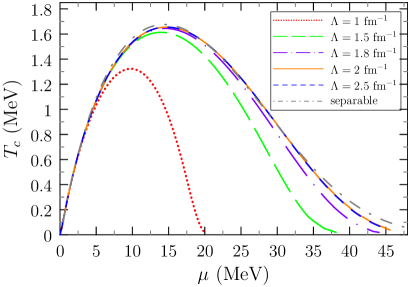
Figure 2: BCS critical temperature $T_{c}$ as a function of the chemical potential $\mu$ for different cutoff values $\Lambda$. The red, green, purple, orange and blue curves correspond to $\Lambda=1$, $1.5$, $1.8$, $2$, and $2.5\;\text{fm}^{-1}$, respectively. The curves obtained for smaller cutoffs are only valid in the range where they agree with the $\Lambda=2$ and $2.5\;\text{fm}^{-1}$ results. The gray curve represents the critical temperature obtained with the separable potential (20).

we display $T_{c}$ as a function of $\mu$, computed with different $V_{\text{low-}k}$ interactions. Matrix elements of the $V_{\text{low-}k}$ interaction are available for arbitrary values of the cutoff $\Lambda$. In our calculations, we use matrix elements of Ref. Ramanan and Urban (2018). For each cutoff, the $V_{\text{low-}k}$ interaction is constructed such that it reproduces the low-energy $nn$ scattering data, but of course only at momenta below that cutoff. Thus the lower cutoffs make only sense for small values of the chemical potential where the cutoff dependence does not yet set in. For $\Lambda\geq 2\;\text{fm}^{-1}$, the $T_{c}$ vs. $\mu$ curve remains unchanged over the whole range of chemical potentials and shows the usual behaviour. For the smaller cutoffs, however, we see that the chemical potential must be limited to $\mu<5\;\text{MeV}$ for $\Lambda=1\;\text{fm}^{-1}$, $\mu<10\;\text{MeV}$ for $\Lambda=1.5\;\text{fm}^{-1}$, and so on, which can be summarized as $\mu[\text{MeV}]\lesssim 4\,(\Lambda[\text{fm}^{-1}])^{2}$. We also display the result obtained with the separable interaction. For $\mu\lesssim 35\;\text{MeV}$, it reproduces well the $V_{\text{low-}k}$ results obtained with $\Lambda=2\;\text{fm}^{-1}$.

III.2 Spectral function and pseudogap

Below the critical temperature $T_{c}$, the pairing gap corresponds to an energy interval around the Fermi energy ($\omega=0$) where there are no states, because adding or removing a particle requires the energy to break a pair. Above $T_{c}$, such a gap does not exist, but in some cases one observes an energy region of reduced density of states, which is called the pseudogap. The spectral function $A(k,\omega)$, Eq. (36), can give give us information on this pseudogap. Figure 3

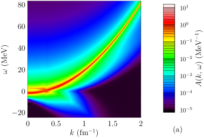
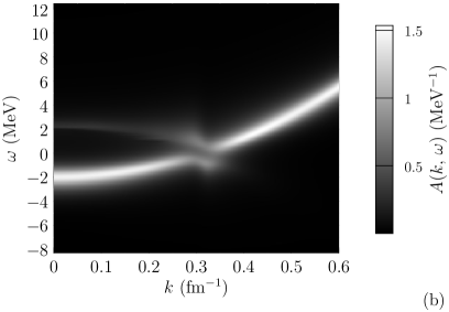
Figure 3: Two-dimensional map of the spectral function $A(k,\omega)$ for $\mu=2\;\text{MeV}$ and $T=1.01\,T_{c}(\mu)$ with the separable interaction. In figure (a), we can clearly see the position of the peak located at $\omega=k^{2}/2-\mu$ and a double-peak structure for $k\lesssim k_{\text{\tiny{F}}}$. Figure (b) is a zoom on the region with the double peak.

displays the spectral function computed for $\mu=2\;\text{MeV}$ at $T=0.53\;\text{MeV}$ which is slightly above $T_{c}$. We can clearly see a double peak for momenta below and around $k_{\text{\tiny{F}}}$, as well as the significant level repulsion between the two peaks near $k=k_{\text{\tiny{F}}}$. Although we are in the normal phase, this behavior reminds the quasiparticle spectrum in BCS theory in the superfluid phase below $T_{c}$, except that the peaks have a width and the spectral function does not vanish between the peaks.

To quantify the presence of the pseudogap, we define the level density

$$N(\omega)=\dfrac{1}{2\pi^{3}}\int_{0}^{\infty}dk\,k^{2}\,A(k,\omega)$$ (38)

Figure 4

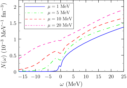
Figure 4: Level densities for several values of the chemical potential $\mu=1\;\text{MeV}$ (blue line), $5\;\text{MeV}$ (green dash-dot line), $10\;\text{MeV}$ (red dashed line) and $20\;\text{MeV}$ (double-dashed purple line) slightly above the respective critical temperatures $T=1.01\,T_{c}(\mu)$ which are $0.27,1.09,1.57$, and $1.53\;\text{MeV}$.

shows the level density calculated for different values of the chemical potential at the corresponding critical temperatures. In all cases, we see a dip in the level density around $\omega=0$. For $\mu=20\;\text{MeV}$, however, this reduction is very weak, because we are no longer in the strong-coupling regime. For $\mu=1\;\text{MeV}$ the dip looks very small, but one has to remember that also the relevant energy scale given by $\mu$ is much smaller.

While, to our knowledge, the pseudogap has not yet been discussed for the case of pure neutron matter, we notice that it was theoretically predicted for the case of dilute symmetric nuclear matter, which undergoes a true crossover from a BEC of deuterons to a BCS phase of $pn$ Cooper pairs Schnell et al. (1999). In ultracold Fermi gases in the BCS-BEC crossover, some hints for the backbending of the peak energy near $k=k_{\text{\tiny{F}}}$ at temperatures above $T_{c}$ were experimentally observed Gaebler et al. (2010). However, even in the unitary Fermi gas, where pairing correlations are stronger than in neutron matter, it is not clear whether the pseudogap phase exists. Theoretically, it tends to be very visible in non self-consistent T-matrix approaches, such as the present one, but less pronounced in self-consistent Green’s functions and quantum Monte-Carlo calculations Jensen et al. (2019). A pseudogap can have some effect on the spin susceptibility and the specific heat Jensen et al. (2020), but in the present case these effects are probably too weak to be observed in neutron stars.

III.3 Occupation numbers

Figure 5

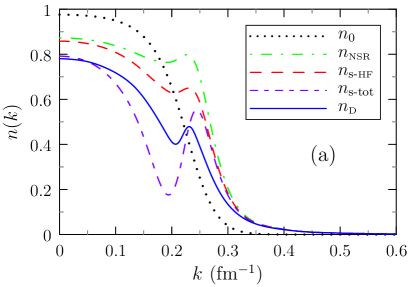
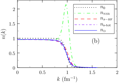
Figure 5: Occupation numbers at $T=1.01\,T_{c}(\mu)$ with (a) $\mu=1\;\text{MeV}$ and (b) $\mu=20\;\text{MeV}$. The dotted black curve represents the free occupation numbers. The green dash-dot curve represents the NSR occupation numbers. The occupation numbers with HF subtraction (s-HF) and total subtraction (s-tot) are represented, respectively, by the red dashed curve and by the purple double dashed curve. Occupation numbers calculated with the full Dyson equation are represented by the blue line.

shows the shape of the occupation numbers, computed at the critical temperature (in practice, slightly above $T_{c}$), for the different approximations defined in Sec. II.5. The left panel (a) was computed with $\mu=1\;\text{MeV}$, where the neutron matter is in a strong-coupling regime since with $T_{c}=0.27\;\text{MeV}$ the ratio $T_{c}/\mu$ is not small. We notice that the occupation numbers including the correlations look all very different from the free ones (dotted black line) but they depend strongly on the choice of the approximation which is used (NSR, subtraction of the HF self-energy, subtraction of the total self-energy, or full Dyson equation).

The right panel (b) was computed with $\mu=20\;\text{MeV}$. In this case, the critical temperature of $T_{c}=1.52\;\text{MeV}$ is close to its maximum, but the ratio $T_{c}/\mu$ is much smaller than for $\mu=1\;\text{MeV}$, and we are therefore more in a weak-coupling situation. In this case, one would expect that BCS theory is valid and the occupation numbers above $T_{c}$ are close to the free ones. As we see from the figure, this is indeed the case for all approximations except NSR. The peak in the NSR occupation numbers is clearly unphysical. When we look at the formula (29), we can see that the derivative of the Fermi function will produce a peak near $k_{\text{\tiny{F}}}$. This has nothing to do with correlations but it simply reflects the shift of the quasiparticle energies, treated to first order in a Taylor expansion. This effect is absent in the other approximations where the chemical potential has to be interpreted as an effective one, $\mu^{\star}$, which already includes the shift, as pointed out below Eq. (31). Therefore, the NSR curve and the other curves are not really comparable as they correspond to different values of the real chemical potentials.

III.4 Correlated density

The main objective of the T-matrix theory is to determine the density dependence of the critical temperature. As mentioned in Sec. III.1, the relation between $T_{c}$ and $\mu$ is the same as in BCS theory, and the effect of the correlations above $T_{c}$ enters only through the $\mu$ dependence of the density $\rho$. The density is calculated directly from the occupation numbers as

$$\rho=2\int\dfrac{d^{3}k}{(2\pi)^{3}}\,n(k)\,,$$ (39)

where the factor of two accounts for the spin degeneracy. As we have seen in Sec. II.5, for the approximations that treat the correlations only perturbatively (NSR, HF subtraction or total subtraction), the density is naturally separated into two parts such that $\rho=\rho_{0}+\rho_{c}$, with $\rho_{0}$ the free density and $\rho_{c}$ the correlated density. In the case of the full Dyson equation, we directly obtain the total occupation numbers and therefore the total density $\rho$. In this case, we define the correlated density as $\rho_{c}=\rho-\rho_{0}$.

The four panels in Fig. 6 represent the ratios $\rho_{c}/\rho_{0}$, computed at the critical temperature $T_{c}(\mu)$, as a function of the chemical potential $\mu$, in the four different approximations: (a) NSR, Eq. (29); (b) HF subtraction, Eq. (33); (c) total subtraction, Eq. (35); and (d) full Dyson equation, Eq. (37).

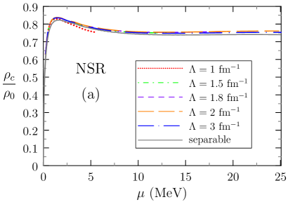
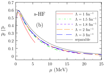
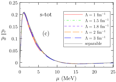
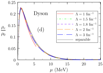
Figure 6: Correlated densities at $T=1.01\,T_{c}(\mu)$ as a function of the chemical potential for four methods to calculate the correlations: (a) NSR, (b) HF subtraction, (c) total self-energy subtraction, and (d) full Dyson equation. The calculations were done with $V_{\text{low-}k}$ interactions corresponding to cutoffs $\Lambda=1$ (red), $1.5$ (green), $1.8$ (purple), $2$ (orange), $3$ (blue), and with the separable interaction (grey curves).

The calculations were done using $V_{\text{low-}k}$ interactions with different cutoffs $\Lambda$ and with the separable interaction. Before we turn to a discussion of the cutoff dependence, let us look at the results obtained with the largest cutoffs $\Lambda=2$ and $3\;\text{fm}$ (orange and blue long dashes), which lie practically on top of each other and are very close to the results obtained with the separable interaction (gray solid lines).

We see that at very small chemical potential, the ratio $\rho_{c}/\rho_{0}$ rises quickly, because the $nn$ scattering length is so large that one quickly gets into the strong-coupling regime. However, what happens at larger chemical potentials depends on the approximation. Since the $nn$ interaction gets weaker at higher momentum, one would expect that neutron matter returns into the weak-coupling regime at high density, i.e., at high chemical potentials, and in this case, the ratio $\rho_{c}/\rho_{0}$ should become small. We see that this is true for all approximations except the NSR one [Fig. 6(a)]. This shows us once again the problem that exists with the NSR theory, namely that it counts the effect of the shift of the quasiparticle energy as “correlations” (or as “fluctuations” in the terminology of Ref. Inotani et al. (2019)). Thus, in the weak coupling limit at large values of the chemical potential, the NSR “correlated density” remains very high whereas it should tend towards zero.

This problem is solved in the other three methods by the subtraction of the quasiparticle energy shift from the self-energy. However, as mentioned in Sec. III.3, some caution should be used when comparing Fig. 6(b-c) with the NSR result in Fig. 6(a), because the chemical potential $\mu$ does not have the same meaning in the two cases. We see that among the three approaches employing a subtraction, subtracting only the HF self-energy [Fig. 6(b)], as it was done in Ramanan and Urban (2013), yields a significantly larger correlated density than the subtraction of the total self-energy [Fig. 6(c)] or the full Dyson equation [Fig. 6(d)]. It is interesting to notice that the last two approximations give almost identical results for $\rho_{c}$ in spite of the different shapes of the corresponding occupation numbers [cf. Fig. 5].

Let us now discuss the results obtained with lower cutoffs $\Lambda=1-1.8\;\text{fm}^{-1}$ (red, green and purple lines in Fig. 6). Keeping in mind the dependence of $T_{c}$ on the cutoff, shown in Fig. 2, we limit these curves to the interval of $\mu$ where $T_{c}$ is cutoff independent. Nevertheless, we notice that the correlated densities depend on the cutoff values, but to a greater or lesser extent depending on the approximation that is used. In the NSR case [Fig. 6(a)], only the $\Lambda=1\;\text{fm}^{-1}$ result deviates significantly from the results obtained with higher cutoffs. The strongest cutoff dependence, even for $\Lambda=1.8\;\text{fm}^{-1}$, can be seen in the calculation using the HF subtraction [Fig. 6(b)], while the cutoff dependence is hardly visible for calculations using total self-energy subtraction [Fig. 6(c)] and the full Dyson equation [Fig. 6(d)]. This can be easily understood because the HF self-energy $\Sigma_{\text{\tiny{HF}}}$, Eq. (25), uses directly the interaction $v$ instead of the T matrix $\Gamma$, but the $V_{\text{low-}k}$ interaction is made such that $\Gamma$ in vacuum is independent of the cutoff, which implies a strong cutoff dependence of $v$ and hence of $\Sigma_{\text{\tiny{HF}}}$. Although the cutoff independence of $\Gamma$ in vacuum does not necessarily ensure the cutoff independence of $\Gamma$ in the medium, we see that the results that employ the full $\Gamma$, i.e., the subtraction of the total self-energy and the full Dyson equation, satisfy the cutoff independence very well. It is, however, not clear why for $\Lambda=1\;\text{fm}^{-1}$, the cutoff dependence of the NSR result sets in already at an unexpectedly small value of $\mu$.

III.5 Density dependence of the critical temperature

Having computed the critical temperature $T_{c}$ and the total density $\rho$ as functions of the chemical potential $\mu$, we can now compute $T_{c}$ as a function $\rho$. To emphasize the low-density behavior, where strong-coupling effects are most pronounced, we show in Fig. 7 the critical temperature $T_{c}$

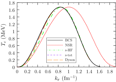
Figure 7: Critical temperature $T_{c}$ as a function of $k_{\text{\tiny{F}}}$ calculated with the separable interaction with different approximations for the density: uncorrelated density (BCS, black solid line), NSR scheme (red dots), HF subtraction (green dashed-dotted curve), subtraction of the total self-energy (purple short dashes), full Dyson equation (orange long dashes).

as a function of the Fermi momentum $k_{\text{\tiny{F}}}$, which is related to $\rho$ by $k_{\text{\tiny{F}}}=(3\pi^{2}\rho)^{1/3}$.

Compared to the BCS result (black curve), which is computed with the uncorrelated density $\rho_{0}$, the curves that account for the correlations in the normal phase are more or less strongly shifted to the right, depending on the correlated density $\rho_{c}$. The fact that the NSR correlated density does not tend towards zero in the high-density limit causes the NSR curve (red) to be shifted even at the highest densities where $T_{c}$ is very low, as it was also found in Ref. Inotani et al. (2019). In the other treatments of the correlations, the curves tend towards the BCS one at high density, which is the expected result since this limit corresponds to the weak-coupling region where the BCS theory should be valid. The correlated densities calculated with the subtraction of the total self-energy (purple) and with the full Dyson equation (orange) being almost identical, it is difficult to distinguish these two curves in Fig. 7.

In order to better see where the weak- and strong coupling regimes are located, we plot in Fig. 8(a) the ratio $T_{c}/E_{\text{\tiny{F}}}$ as a function of $k_{\text{\tiny{F}}}$, where $E_{\text{\tiny{F}}}=\hbar^{2}k_{\text{\tiny{F}}}^{2}/(2m)$ denotes the Fermi energy.

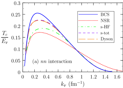
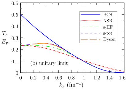
Figure 8: Ratio $T_{c}/E_{\text{\tiny{F}}}$ as a function of $k_{\text{\tiny{F}}}$ for the separable interaction. The blue solid curve represents the free case (BCS), the red dotted curve the NSR case, the green dashed-dotted curve the HF subtraction, the purple short dashed curve the subtraction of the total self-energy, and the orange long dashed curve the density obtained with the full Dyson equation. Panel (a) shows results for the physical $nn$ interaction, while panel (b) shows results for the interaction that was readjusted to give an infinite $nn$ scattering length (unitary limit).

The BCS theory should hold in the weak-coupling limit $T_{c}/E_{\text{\tiny{F}}}\ll 1$. Therefore, largest deviation from the BCS solid curve (blue) should be seen around $k_{\text{\tiny{F}}}\approx 0.3\;\text{fm}^{-1}$, where the ratio $T_{c}/E_{\text{\tiny{F}}}$ has its maximum. Again, as discussed above, the NSR dotted curve (red) is the only one that does not tend towards the BCS curve at high density. In the case of HF subtraction (green short dashed curve), used in Ref. Ramanan and Urban (2013), a significant reduction of $T_{c}$ compared to the BCS one is seen in the interval $k_{\text{\tiny{F}}}\approx 0.1-0.8\;\text{fm}^{-1}$ ($\rho\approx 5\cdot 10^{-5}-2\cdot 10^{-2}\;\text{fm}^{-3}$), and the reduction can be up to $\sim 30\,\%$. With the subtraction of the total self-energy (purple short dashed curve) or the full Dyson equation (orange long dashed curve), a significant deviation from the BCS result is observed only in the smaller interval $k_{\text{\tiny{F}}}\approx 0.1-0.6\;\text{fm}^{-1}$ (i.e., $\rho\sim 5\cdot 10^{-5}-7\cdot 10^{-3}\;\text{fm}^{-3}$) and the reduction is at most $\sim 12\,\%$.

The small correlated densities that we get with the subtraction of the total self-energy or with the Dyson equation are quite astonishing. In ultracold atoms (i.e., with a contact interaction) in the unitary limit, the experimental result is $T_{c}/E_{\text{\tiny{F}}}\simeq 0.16$ Nascimbène et al. (2010); Ku et al. (2012), while the BCS theory predicts $T_{c}/E_{\text{\tiny{F}}}\simeq 0.5$. A large part of the observed suppression is believed to come from the correlated pairs above $T_{c}$, for instance with NSR one finds $T_{c}/E_{\text{\tiny{F}}}\simeq 0.23$ Sá de Melo et al. (1993), i.e., a suppression by more than $50\,\%$ compared to BCS. The remaining reduction could be, e.g., due to screening effects Pisani et al. (2018), but within the self-consistent Green’s function formalism one finds $T_{c}/E_{\text{\tiny{F}}}\simeq 0.16$ even though screening is not included Haussmann et al. (2007).

Let us therefore test our methods by verifying that we reproduce the known results. To that end, we repeat the calculations with the modified value of the coupling constant $g$ of the separable interaction corresponding to the unitary limit given in Table 1. Figure 8(b) shows us the ratio $T_{c}/E_{\text{\tiny{F}}}$ as a function of $k_{\text{\tiny{F}}}$ for this case. We notice that $T_{c}/E_{\text{\tiny{F}}}$ remains finite even in the limit $k_{\text{\tiny{F}}}\to 0$. This is a peculiarity of the unitary limit, because the dimensionless parameter $k_{\text{\tiny{F}}}a$ remains infinite independently of the value of $k_{\text{\tiny{F}}}$. However, the finite range $r_{0}$ of the interaction becomes negligible in this limit because the relevant dimensionless combination $k_{F}r_{0}$ tends to zero. Hence, in the limit $k_{\text{\tiny{F}}}\to 0$, our results reproduce those obtained in ultracold atoms with a contact interaction: In BCS, we find $T_{c}/E_{\text{\tiny{F}}}\simeq 0.5$ and in the correlated cases (NSR, HF subtraction, total self-energy subtraction, and full Dyson equation) we find $T_{c}/E_{\text{\tiny{F}}}\simeq 0.23$ which is compatible with the results obtained in Sá de Melo et al. (1993) for NSR and in Pantel et al. (2014) for the subtraction of the total self-energy (denoted there Zimmermann-Stolz (ZS) scheme after Ref. Zimmermann and Stolz (1985)).

For finite values of $k_{\text{\tiny{F}}}$, the interaction gets weaker because of its momentum dependence, and we expect that, as a function of $k_{\text{\tiny{F}}}$, we should find a similar behavior as if one increases the parameter $-1/(k_{\text{\tiny{F}}}a)$ in the BEC-BCS crossover of cold atoms. All curves except the NSR one tend towards the BCS result. We also find that the behavior of the curves for NSR and total self-energy subtraction is similar to that obtained in cold atoms, namely that the NSR curve is strictly increasing with increasing interaction on the BCS side (since the maximum lies on the BEC side Sá de Melo et al. (1993)), while the curve for total self-energy subtraction has its maximum on the BCS side Pantel et al. (2014).

From this comparison we conclude that the smallness of the correlation correction that we find in Fig. 8(a) is a consequence of the finite scattering length $a=-15.9\;\text{fm}$ of the realistic separable interaction. Although this value is quite large compared to other nuclear scales, the parameter $k_{\text{\tiny{F}}}a$ gets only large when the finite range of the interaction already starts to weaken it, so that the BCS-BEC crossover effects remain rather weak.

IV Open questions

IV.1 Problem of the subtraction

In Sec. II.5, we argued that in a non-self-consistent treatment of the propagators, we have to subtract from the self-energy the mean-field like quantity $\Sigma(k,\xi_{k})$. In Fig. 9, we represent the momentum dependence of this shift in the case of the separable interaction.

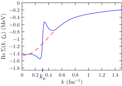
Figure 9: Real part of the on-shell self-energy $\Sigma(k,\xi_{k})$ as a function of $k$ for $\mu=2\;\text{MeV}$ and $T=1.01\,T_{c}(\mu)=0.53\;\text{MeV}$, computed with the separable interaction (blue curve). The value of $k_{\mu}=\sqrt{2m\smash{\mu}}/\hbar$ approximates the position of the Fermi surface. The red dotted line is not the result of a calculation but it is drawn by hand to show schematically how a more appropriate subtraction could look like.

By defining $k_{\mu}=\sqrt{2m\smash{\mu}}/\hbar$ which roughly indicates the position of the Fermi surface, we notice a big jump in this region. It is clear that a momentum dependent mean field as computed with, e.g., a Skyrme or Gogny interaction, would never have such a shape. We suspect that by doing this subtraction, while computing the internal propagators in $\Gamma$ and $\Sigma$ with the free dispersion relation, we remove parts of the physical effects caused by the self-energy. It seems probable that this subtraction, as it was implicitly also used in Zimmermann and Stolz (1985); Schmidt et al. (1990); Stein et al. (1995); Jin et al. (2010); Pantel et al. (2014), reduces the pseudogap and the correlated densities. We notice that in the literature there are other possible ways to do this subtraction. One of them, used in Perali et al. (2002); Pieri et al. (2004), consists in neglecting the momentum dependence and taking it at $k=k_{\mu}$, i.e., subtracting a constant $\Sigma_{0}=\operatorname{Re}\Sigma(k_{\mu},0)$. Looking at the graph, we see that this is problematic, too, because the subtraction is precisely fixed in the zone of the jump where the function varies rapidly, so that the value of the subtraction depends very sensitively on the approximation. Qualitatively, we think that it would be more appropriate to subtract a smooth curve as schematically represented in Fig. 9 by the red dotted line.

IV.2 Effect of the quasiparticle weight

In Ref. Cao et al. (2006), a new effect was discussed that strongly reduces the critical temperature, namely the reduced quasiparticle weight. It is well known that the Cooper instability comes from the jump of the Pauli factor $1-f_{\text{\tiny{F}}}(\xi_{\textbf{\text{k}}/2+\mathbf{p}})-f_{\text{\tiny{F}}}(\xi_{\textbf{\text{k}}/2-\mathbf{p}})$ in the numerator of Eq. (3) at $p=k_{\mu}$ for $k=0$. However, this Pauli factor is obtained with uncorrelated Green’s functions having a quasiparticle weight of unity, $Z=1$. In Ref. Cao et al. (2006), it was argued that the amplitude of the jump should be multiplied by the quasiparticle weight $Z<1$, which in that work was determined from a Brückner calculation.

A more self-consistent method to include this effect would be the so-called renormalized RPA (r-RPA) Schuck et al. (2020), where, in the particle-particle channel, the Pauli factor is replaced by

$$1-f_{\text{\tiny{F}}}(\xi_{\textbf{\text{k}}/2+\mathbf{p}})-f_{\text{\tiny{F}}}(\xi_{\textbf{\text{k}}/2-\mathbf{p}})\to 1-n(\textbf{\text{k}}/2+\mathbf{p})-n(\textbf{\text{k}}/2-\mathbf{p})\,,$$ (40)

with $n(k)$ the correlated occupation numbers, which should be calculated self-consistently. At zero-temperature, the correlated occupation numbers have a jump of height $Z$ at $k=k_{\text{\tiny{F}}}$ and therefore the height of the jump of the Pauli factor is also reduced by a factor of $Z$. We recently applied this method to the case of strongly polarized Fermi gases at zero temperature Durel and Urban (2020) where it reduces the critical polarization, which plays a similar role as the critical temperature in the present case.

However, here it turns out that it is not possible to realize a self-consistent calculation of r-RPA type. When we insert the correlated occupation numbers in the Pauli factor $\bar{Q}(k,p)$, it does no longer vanish at $p=k_{\mu}$, leading to a non-vanishing imaginary part of the vertex function $\Gamma$ at $\omega=0$. This makes it impossible to calculate the self-energy, as one can see from Eq. (26): $\operatorname{Im}\Gamma$ must vanish where the Bose function $f_{\text{\tiny{B}}}$ diverges.

Despite this problem, let us estimate the order of magnitude of the effect. To that end, we replace in the angle averaged Pauli factor $\bar{Q}$ the free occupation numbers by the correlated ones according to Eq. (40), calculated with the full Dyson equation with the separable interaction. For this choice, in certain regions (in the not too strongly coupled regime), the imaginary part of $\operatorname{Im}J(k=0,\omega)$ [cf. Eq. (22)] changes sign almost at $\omega=0$ so that we can try to estimate the critical temperature from $\operatorname{Re}J(k=0,\,\omega=0\,;\,T=T_{c})=1/g$ [cf. Eq. (21)].

This is illustrated in Fig. 10.

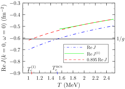
Figure 10: Real part of $J(k=0,\,\omega=0)$ for $\mu=20$ MeV as a function of the temperature $T$. The blue dash-dot curve represents the usual calculation, using $\bar{Q}$ according to Eq. (5), while the the green curve displays $J^{(1)}$ which is obtained when the Fermi functions in the Pauli factor are replaced according to Eq. (40). The red dashed curve is an extrapolation of $J^{(1)}$ down to $T_{c}^{(1)}$ under the assumption that it has the same form as $J$.

Notice that the occupation numbers $n(k)$ used in Eq. (40) are computed with the ordinary $J$ and not self-consistently, because, as mentioned above, we cannot compute the self-energy with the modified $J$. Hence, our modified $J$, denoted $J^{(1)}$, can be regarded as a first step of a self-consistent iteration. Furthermore, as it is impossible to compute the correlated occupation numbers below $T_{c}^{\text{\tiny{BCS}}}$, it is necessary to extrapolate $J^{(1)}$ to the new critical temperature $T_{c}^{(1)}$. In the example $\mu=20$ MeV presented in Fig. 10, we find that at temperatures not too close to $T_{c}^{\text{\tiny{BCS}}}$ this effect reduces $\operatorname{Re}J(0,0)$ by about $10\,\%$, reducing $T_{c}$ by about $30\,\%$. Although this is only a rough estimate, it indicates that this effect might be important.

V Conclusions

The in-medium T-matrix formalism makes it possible to describe pair correlations in neutron matter. To model the $nn$ interaction, we use the effective low-momentum interaction $V_{\text{low-}k}$. We presented a numerical method to solve the integral equation for the vertex function $\Gamma$. It is also possible to replace $V_{\text{low-}k}$ by a separable interaction which gives very similar results and largely facilitates the numerical computations.

Because of the large $nn$ scattering length, it is believed that dilute neutron matter is close to the unitary Fermi gas and that BCS-BEC crossover physics plays an important role. We pointed out that the standard NSR theory, which is widely used for the BCS-BEC crossover, has the shortcoming not to tend towards the weak-coupling BCS theory at high density. It leads to unphysical occupation numbers and to an incorrect shift of the $T_{c}$ vs. $\rho$ curve, because it attributes the mean-field like shift of the quasiparticle energy to the correlations.

We compared different prescriptions to avoid these deficiencies by subtracting this shift from the dynamical (i.e., energy dependent) part of the self-energy. Subtracting only the Hartree-Fock (HF) part, as in Ref. Ramanan and Urban (2013), is already enough to make the correlations tend towards zero in the weak-coupling limit. To go beyond this approximation, we subtract the total on-shell self-energy, as implicitly done within the Zimmermann-Stolz scheme Zimmermann and Stolz (1985) which was previously used for the description of the BCS-BEC crossover in dilute symmetric nuclear matter Schmidt et al. (1990); Stein et al. (1995); Jin et al. (2010). This prescription avoids the unphysical dependence of the HF subtraction on the cutoff of the $V_{\text{low-}k}$ interaction, but has the effect of further reducing the correlations and therefore the crossover effects. With the explicit calculation of the self-energy, we are also able to calculate the correlations through the full Dyson equation and not just its truncation to the first order as it is customary to do. This method gives us access to the spectral function and allows us to highlight the existence of a pseudo-gap in neutron matter above $T_{c}$. As discussed in Sec. IV.1, it is possible that we underestimate the pseudogap as a consequence of the subtraction method.

At a quantitative level, it seems that the suppression of the critical temperature for a given density, due to the density of preformed pairs, is too weak to have much effect on neutron-star observables. However, a more important effect is expected to result from the quasiparticle weight $Z<1$, as also pointed out in Ref. Cao et al. (2006). In the weak-coupling regime we estimate that this effect may reduce $T_{c}$ by $\sim 30\,\%$, but our present theory does not allow us to compute it self-consistently or in the strong-coupling regime.

Finally, a large uncertainty comes from screening of the bare $nn$ interaction in the medium Cao et al. (2006); Ramanan and Urban (2018); Urban and Ramanan (2020) which is not included in the present study. These effects depend sensitively on the approximations that are used, on the Landau parameters and on the momentum dependence of the effective interaction used in the residual particle-hole interaction. From the results of Ref. Urban and Ramanan (2020), it seems most likely that in the low-density region corresponding to the strong-coupling regime, screening suppresses the critical temperature by about $30-40\,\%$, thereby reducing further the crossover effects.

References

- Chamel and Haensel (2008) N. Chamel and P. Haensel, Living Reviews in Relativity 11, 10 (2008).
- Abe and Seki (2009) T. Abe and R. Seki, Phys. Rev. C 79, 054002 (2009).
- Gezerlis and Carlson (2010) A. Gezerlis and J. Carlson, Phys. Rev. C 81, 025803 (2010).
- Okihashi and Matsuo (2020) T. Okihashi and M. Matsuo, ArXiv e-prints (2020), eprint 2009.11505.
- Chamel et al. (2010) N. Chamel, S. Goriely, J. M. Pearson, and M. Onsi, Phys. Rev. C 81, 045804 (2010).
- González Trotter et al. (1999) D. E. González Trotter, F. Salinas, Q. Chen, A. S. Crowell, W. Glöckle, C. R. Howell, C. D. Roper, D. Schmidt, I. Šlaus, H. Tang, et al., Phys. Rev. Lett. 83, 3788 (1999).
- Babenko and Petrov (2013) V. Babenko and N. Petrov, Phys. Atom. Nuclei 76, 684 (2013).
- Baker (1999) G. A. Baker, Phys. Rev. C 60, 054311 (1999).
- Calvanese Strinati et al. (2018) G. Calvanese Strinati, P. Pieri, G. Röpke, P. Schuck, and M. Urban, Phys. Rep. 738, 1 (2018).
- Nozières and Schmitt-Rink (1985) P. Nozières and S. Schmitt-Rink, J. Low Temp. Phys. 59, 195 (1985).
- Baldo et al. (1995) M. Baldo, U. Lombardo, and P. Schuck, Phys. Rev. C 52, 975 (1995).
- Schmidt et al. (1990) M. Schmidt, G. Röpke, and H. Schulz, Annals of Physics 202, 57 (1990).
- Stein et al. (1995) H. Stein, A. Schnell, T. Alm, and G. Röpke, Z. Phys. A 351, 295 (1995).
- Jin et al. (2010) M. Jin, M. Urban, and P. Schuck, Phys. Rev. C 82, 024911 (2010).
- Matsuo (2006) M. Matsuo, Phys. Rev. C 73, 044309 (2006).
- Ramanan and Urban (2013) S. Ramanan and M. Urban, Phys. Rev. C 88, 054315 (2013).
- Ramanan and Urban (2018) S. Ramanan and M. Urban, Phys. Rev. C 98, 024314 (2018).
- Tajima et al. (2019) H. Tajima, T. Hatsuda, P. van Wyk, and Y. Ohashi, Scientific Reports 9 (2019).
- Urban and Ramanan (2020) M. Urban and S. Ramanan, Phys. Rev. C 101, 035803 (2020).
- Ohashi et al. (2020) Y. Ohashi, H. Tajima, and P. van Wyk, Prog. Part. Nucl. Phys. 111, 103739 (2020).
- Inotani et al. (2019) D. Inotani, S. Yasui, and M. Nitta, ArXiv e-prints (2019), eprint 1912.12420v1.
- Sá de Melo et al. (1993) C. A. R. Sá de Melo, M. Randeria, and J. R. Engelbrecht, Phys. Rev. Lett. 71, 3202 (1993).
- Bogner et al. (2010) S. Bogner, R. Furnstahl, and A. Schwenk, Prog. Part. Nucl. Phys. 65, 94 (2010).
- Holt et al. (2010) J. W. Holt, N. Kaiser, and W. Weise, Phys. Rev. C 81, 024002 (2010).
- Fetter and Walecka (1971) A. L. Fetter and J. D. Walecka, Quantum Theory of Many-Particle Systems (McGraw-Hill, New York, 1971).
- Weinberg (1963) S. Weinberg, Phys. Rev. 131, 440 (1963).
- Törnig and Spellucci (1990) W. Törnig and P. Spellucci, Numerische Mathematik für Ingenieure und Physiker (Springer, Berlin, 1990).
- Thouless (1960) D. J. Thouless, Annals of Physics 10, 553 (1960).
- Khodel et al. (1996) V. A. Khodel, V. V. Khodel, and J. W. Clark, Nucl. Phys. A 598, 390 (1996).
- Martin and Urban (2014) N. Martin and M. Urban, Phys. Rev. C 90, 065805 (2014).
- Zimmermann and Stolz (1985) R. Zimmermann and H. Stolz, Phys. Status Solidi B 131, 151 (1985).
- Haussmann et al. (2007) R. Haussmann, W. Rantner, S. Cerrito, and W. Zwerger, Phys. Rev. A 75, 023610 (2007).
- Buraczynski et al. (2019) M. Buraczynski, N. Ismail, and A. Gezerlis, Phys. Rev. Lett. 122, 152701 (2019).
- Schnell et al. (1999) A. Schnell, G. Röpke, and P. Schuck, Phys. Rev. Lett. 83, 1926 (1999).
- Gaebler et al. (2010) J. P. Gaebler, J. T. Stewart, T. E. Drake, D. S. Jin, A. Perali, P. Pieri, and G. C. Strinati, Nature Physics 6, 659 (2010).
- Jensen et al. (2019) S. Jensen, C. Gilbreth, and Y. Alhassid, Eur. Phys. J. ST 227, 2241 (2019).
- Jensen et al. (2020) S. Jensen, C. N. Gilbreth, and Y. Alhassid, Phys. Rev. Lett. 124, 090604 (2020).
- Nascimbène et al. (2010) S. Nascimbène, N. Navon, K. J. Jiang, F. Chevy, and C. Salomon, Nature 463, 1057 (2010).
- Ku et al. (2012) M. J. H. Ku, A. T. Sommer, L. W. Cheuk, and M. W. Zwierlein, Science 335, 563 (2012).
- Pisani et al. (2018) L. Pisani, A. Perali, P. Pieri, and G. C. Strinati, Phys. Rev. B 97, 014528 (2018).
- Pantel et al. (2014) P.-A. Pantel, D. Davesne, and M. Urban, Phys. Rev. A 90, 053629 (2014), erratum ibid. 2016, 94, 019901.
- Perali et al. (2002) A. Perali, P. Pieri, G. C. Strinati, and C. Castellani, Phys. Rev. B 66, 024510 (2002).
- Pieri et al. (2004) P. Pieri, L. Pisani, and G. C. Strinati, Phys. Rev. B 70, 094508 (2004).
- Cao et al. (2006) L. G. Cao, U. Lombardo, and P. Schuck, Phys. Rev. C 74, 064301 (2006).
- Schuck et al. (2020) P. Schuck, D. S. Delion, J. Dukelsky, M. Jemai, E. Litvinova, G. Röpke, and M. Tohyama, ArXiv e-prints (2020), eprint 2009.00591.
- Durel and Urban (2020) D. Durel and M. Urban, Phys. Rev. A 101, 013608 (2020).