Black Holes in Double-Logarithmic Nonlinear Electrodynamics

Abstract

The electric and magnetic black hole solutions are found by coupling the recently introduced nonlinear electrodynamics (NED) model, called “double logharitmic nonlinear electrodynamics” with cosmological Einstein gravity. The solutions become Reissner-Nordstrom (RN) black hole in the weak field limit and asymptotically. The electric solution is expressed as an integral equation while the magnetic black hole solution is expressed in terms of elementary functions. Hence, the thermodynamic structure of the magnetic black hole solution is analyzed by deriving the modified Smarr’s formula and studying the first law of thermodynamics. Moreover, its stability is investigated by deriving the heat capacity.

I Introduction

In early time cosmology the problem of big bang singularity and inflation are still contemporary. Nonlinear electrodynamics (NED) maybe a solution to these problems. The gravitational fields and electromagnetic fields were very strong in creation of the universe. There is an inextricable relation between strong fields and nonlinearities therefore the nonlinear effects not only took an important role in early time universe but also are crucial in understanding black hole singularities.

As a NED Born-Infeld (BI) electrodynamics Born ; Born-Infeld , whose action comes out from low energy effective action of superstring theory Fradkin-Tseytlin ; Tseytlin , solves the problem of singularity of the electric field at the center of a charged point particle, therefore the electric energy of charged particles becomes finite. Beside BI, some models of NED are introduced in Gitman-Shabad ; Kruglov-1 ; Kruglov-2 ; Kruglov-3 ; Gullu-Mazharimousavi and these models are free of singularity of the electric field at the center of charged particles. At the weak field limit BI theory goes to Maxwell electrodynamics which can be thought as an approximation of NED.

The properties of NED can be comprehensible in the framework of gravity since, strong electromagnetic fields are dominant in the early period of the universe, at the center of black holes and charged particles. The exact black hole solution in General Relativity (GR) was given in Oliveira by use of a NED Lagrangian which defines a large class of non-linear theories including BI and Euler-Heisenberg (EH) electrodynamics whose weak field limit also tends to Maxwell electrodynamics. Other models of NED coupled to gravity have been studied in Ayon-Beato-Garcia ; Breton-1 ; Dymnikova ; Balart-Vagenas ; Kruglov-4 . The solution of these models are singularity free black hole solutions which asymptotically behave as the Raisner-Nördstrom (RN) black hole Reissner ; Nordstrom . There is already a rich literature in this respect as contributions of NED models in the formation of different type black holes Fernando-Krug -Kruglov-13 . Moreover, instead of dark energy, non-linear electromagnetic fields are introduced to explain the inflation period in early time universe Garcia-Breton ; Camara-et.al. . In addition, some models of NED were used to depict accelerated expansion of the universe Elizalde-et.al. ; Novello-et.al.-1 ; Novello-et.al.-2 ; Vollick ; Kruglov-5 ; Kruglov-6 . In $\Lambda$-Cold Dark Matter ($\Lambda$CDM) model the expansion of the universe is driven by the cosmological constant $\Lambda$, on the other hand the non-zero trace of the energy-momentum tensor in NED can play the role of cosmological constant Labun ; Schutzhold .

In this paper we consider a recently introduced NED model Gullu-Mazharimousavi , which is constructed by both Maxwell (Lorentz) invariants $\mathcal{F}=F^{\mu\nu}F_{\mu\nu}$ and $\mathcal{G}=F_{\mu\nu}\tilde{F}^{\mu\nu}$ and carries one dimensional parameter $\beta$, and couple it to the gravitational field. Due to the technical difficulty of finding a dyonic black hole solution in which the electric and magnetic fields coexist, we have found electric and magnetic black hole solutions separately in the absence of the second invariant term, $\mathcal{G}$, in the model. The solutions are in the form of modified RN black hole for both cases. We find the electric type black hole solution by setting the magnetic field to zero and letting the source to be electrically charged. The solution is inexact namely, it can only be expressed as an integral expression therefore its series expansion can be of any use. In the second case the electric field is set to zero and the source of gravitational field becomes magnetized and the magnetic black hole solution is exact. Due to this property, the magnetic black hole solution is analyzed in more detail. The first law of thermodynamics, Hawking radiation, the extension of Smarr’s formula and thermal stability are worked out for the magnetic black hole solution Smarr ; Breton-2 ; Rasheed ; Zhang-Gao ; Hu-Kuang-Ong ; Wang-Wu-Yang .

The layout of the paper is as follows: In Section 2 we review the NED model under consideration. In Section 3 electric and magnetic type solutions are found by coupling minimally nonlinear electromagnetic fields to gravitational fields. The thermodynamic properties of the magnetic type solution is investigated in Section 4. Thermal stability of the magnetic black hole constitute the subject for Section 5. The paper is brought to completion with the Conclusion in Section 6.

In the continuation, we take $\hbar=c=\varepsilon_{0}=\mu_{0}=1$ and the metric with mostly plus signature. The coordinates are defined as $x^{\mu}=\left(t,r,\theta,\phi\right)$. Greek indices run from $0$ to $3$ and Latin indices run from $1$ to $3$.

II The New NED Model:

The Double-Logarithmic Lagrangian Gullu-Mazharimousavi is given by

$$\mathcal{L}_{e} =\frac{1}{2\beta}\left[\left(1-\sqrt{-2\beta\mathcal{F}}\right)\ln\left(1-\sqrt{-2\beta\mathcal{F}}\right)+\left(1+\sqrt{-2\beta\mathcal{F}}\right)\ln\left(1+\sqrt{-2\beta\mathcal{F}}\right)\right],$$ (1)

in which $\mathcal{F}=F_{\mu\nu}F^{\mu\nu}=2\left(\boldsymbol{B}^{2}-\boldsymbol{E}^{2}\right)$ is the Maxwell invariant and the electromagnetic strength tensor is given in terms of the gauge potential $F_{\mu\nu}=\partial_{\mu}A_{\nu}-\partial_{\nu}A_{\mu}$ which in the matrix form reads

$$F_{\mu\nu}= \left(\begin{array}[]{cccc}0&E_{r}&0&0\\ -E_{r}&0&0&0\\ 0&0&0&-B_{r}r^{2}\sin\theta\\ 0&0&B_{r}r^{2}\sin\theta&0\end{array}\right),$$ (6)

$$F^{\mu\nu}= \left(\begin{array}[]{cccc}0&-E_{r}&0&0\\ E_{r}&0&0&0\\ 0&0&0&-\frac{B_{r}}{r^{2}\sin\theta}\\ 0&0&\frac{B_{r}}{r^{2}\sin\theta}&0\end{array}\right),$$ (11)

where the electric field and magnetic field are static and depend only on the radial coordinate. In the following computation we need also,

$$F_{\mu\lambda}F^{\nu\lambda}= \left(\begin{array}[]{cccc}-E_{r}^{2}&0&0&0\\ 0&-E_{r}^{2}&0&0\\ 0&0&B_{r}^{2}&0\\ 0&0&0&B_{r}^{2}\end{array}\right).$$ (16)

In the weak field limit $\beta\rightarrow 0$, (1) reduces to the linear Maxwell Lagrangian

$$-\mathcal{F}+\frac{1}{3}\mathcal{F}^{2}\beta-\frac{4}{15}\mathcal{F}^{3}\beta^{2}+O[\beta]^{5/2}.$$ (17)

where the zeroth order term is the usual Maxwell’s theory which can be achieved when $\beta=0$. The first order correction to the Maxwell’s theory is $\frac{1}{3}\mathcal{F}^{2}$. The Lagrangian for the gravity part is the cosmological Einstein-Hilbert Lagrangian

$$\mathcal{L}_{g}=R-2\Lambda,$$ (18)

where $\Lambda$ is the cosmological constant and the action in which the electromagnetic field couples minimally to the gravity field reads as

$$I=\int d^{4}x\sqrt{-g}\left(\frac{1}{2\kappa}\mathcal{L}_{g}+\mathcal{L}_{e}\right),$$ (19)

where $\kappa=8\pi G$ and $G$ is the four dimensional Newton’s constant. The static spherically symmetric line element is chosen to be

$$ds^{2}= -f\left(r\right)dt^{2}+\frac{1}{f\left(r\right)}dr^{2}+r^{2}d\Omega^{2},$$ (20)

in which $d\Omega=d\theta^{2}+\sin^{2}\theta d\phi^{2}$. The field equations of gravitational and electromagnetic fields are

$$\mathcal{G}_{\mu}^{\nu}= \kappa T_{\mu}^{\nu},$$ (21)

where the cosmological Einstein tensor reads $\mathcal{G}_{\mu}^{\nu}=G_{\mu}^{\nu}-\Lambda\delta_{\mu}^{\nu}$ with the Einstein tensor $G_{\mu}^{\nu}=R_{\mu}^{\nu}-\frac{1}{2}\delta_{\mu}^{\nu}R$ and the energy-momentum tensor is defined to be

$$T_{\mu}^{\nu}\equiv\mathcal{L}\delta_{\mu}^{\nu}-4\mathcal{L}_{\mathcal{F}}F_{\mu\lambda}F^{\nu\lambda}$$ (22)

which results in

$$T_{\mu}^{\nu}= \frac{1}{2\beta}\left[\left(1-\sqrt{-2\beta\mathcal{F}}\right)\ln\left(1-\sqrt{-2\beta\mathcal{F}}\right)+\left(1+\sqrt{-2\beta\mathcal{F}}\right)\ln\left(1+\sqrt{-2\beta\mathcal{F}}\right)\right]\delta_{\mu}^{\nu}$$

$$-\frac{2F_{\mu\lambda}F^{\nu\lambda}}{\sqrt{-2\beta\mathcal{F}}}\ln\left(\frac{1-\sqrt{-2\beta\mathcal{F}}}{1+\sqrt{-2\beta\mathcal{F}}}\right),$$ (23)

and the second field equation reads

$$\partial_{\alpha}\left\{\frac{\sqrt{-g}}{\sqrt{-2\beta\mathcal{F}}}\ln\left(\frac{1-\sqrt{-2\beta\mathcal{F}}}{1+\sqrt{-2\beta\mathcal{F}}}\right)F^{\alpha\beta}\right\}= 0$$ (24)

after varying the action (19) with respect to the gauge potential $A_{\mu}$. For the metric (20) the components of the cosmological Einstein tensor becomes

$$\mathcal{G}_{0}^{0}=\mathcal{G}_{1}^{1}= \frac{rf^{\prime}\left(r\right)+f\left(r\right)-1-r^{2}\Lambda}{r^{2}}$$

$$\mathcal{G}_{2}^{2}=\mathcal{G}_{3}^{3}= \frac{rf^{\prime\prime}\left(r\right)+2f^{\prime}\left(r\right)-2\Lambda r}{2r}$$ (25)

which will be needed for later use.

III Electric Part:

In this section we find the electric field of a point charge and the electric black hole solution for $B_{r}=0$ which means we have only electric monopole sitting at the origin.

III.1 The Electric Field:

The electric field of a point charge can be found by use of (24). The Maxwell invariant depends only on the Electric field, $\mathcal{F}=-2E_{r}^{2}$, and the electric field has just radial component $\boldsymbol{E}=\left(E_{r}\left(r\right),\,0,\,0\right)$. The determinant of the metric tensor (20) is

$$\sqrt{-g}= r^{2}\sin\theta.$$ (26)

Once the index $\beta$ is taken to be zero, then (24) reduces to

$$\partial_{r}\left\{\frac{r^{2}}{\sqrt{\beta}}\left(\tanh^{-1}\left(\sqrt{\beta}E_{r}\left(r\right)\right)\right)\right\} =0.$$ (27)

The terms inside the parenthesis in (27) are equal to a constant. Then, the electric field of a point particle reads

$$E_{r}\left(r\right)= \frac{1}{2\sqrt{\beta}}\tanh\left(\frac{2\sqrt{\beta}q}{r^{2}}\right),$$ (28)

where $q$ is a constant corresponding to the electric charge of the black hole. In the weak field limit $\beta\rightarrow 0$ the electric field reduces to Coulomb’s field i.e., $E_{r}=\frac{q}{r^{2}}$.

III.2 The Electric Black Hole Solution:

In this part we will solve the Einstein field equations (21) upon use of (20). The energy-momentum tensor reads explicitly

$$T_{\mu}^{\nu}= \mathcal{A}\delta_{\mu}^{\nu}-\mathcal{B}F_{\mu\lambda}F^{\nu\lambda},$$ (29)

where we have defined

$$\mathcal{A}\equiv \frac{1}{2\beta}\left[\left(1-2\sqrt{\beta}E_{r}\right)\ln\left(1-2\sqrt{\beta}E_{r}\right)+\left(1+2\sqrt{\beta}E_{r}\right)\ln\left(1+2\sqrt{\beta}E_{r}\right)\right],$$ (30)

$$\mathcal{B}\equiv \frac{1}{\sqrt{\beta}E_{r}}\ln\left(\frac{1-2\sqrt{\beta}E_{r}}{1+2\sqrt{\beta}E_{r}}\right).$$ (31)

Then, (21) reduces to the first order differential equation given by

$$f^{\prime}\left(r\right)r+f\left(r\right)-\Lambda r^{2}-1= \frac{\kappa r^{2}}{2\beta}\ln\left(1-4\beta E_{r}^{2}\right).$$ (32)

Rewriting (32) as

$$\left(f\left(r\right)r\right)^{\prime}= \frac{\kappa r^{2}}{2\beta}\ln\left(\text{sech}^{2}\left(\frac{2\sqrt{\beta}q}{r^{2}}\right)\right)+\Lambda r^{2}+1$$ (33)

where we have used (28) and the trigonometric identity $\text{sech}^{2}x=1-\tanh^{2}x$. Integrating both sides of (33) one gets the solution of electric black hole as follows

$$f\left(r\right)= \frac{\kappa}{2\beta r}\int r^{2}\ln\left(\text{sech}^{2}\left(\frac{2\sqrt{\beta}q}{r^{2}}\right)\right)dr+\frac{\Lambda r^{2}}{3}+1-\frac{2GM}{r},$$ (34)

where the integration constant is defined as

$$C=2GM,$$ (35)

in which $M$ represents the Schwarzschield mass when there is no electromagnetic field. This solution can be numerically analyzed because the integral can not be expressed in terms of elementary functions. After expanding (34) in Taylor series expansion around $\beta=0$ up to the first order we get

$$f\left(r\right)= 1-\frac{2MG}{r}+\frac{2\kappa q^{2}}{r^{2}}+\frac{\Lambda}{3}r^{2}-\frac{4\kappa q^{4}\beta}{15r^{6}}-\frac{2G}{\beta r}\int r^{2}\mathcal{O}\left(\beta\right)^{\frac{3}{2}}dr.$$ (36)

Setting $\beta=0$ the solution (36) reduces to

$$f\left(r\right)= 1-\frac{2MG}{r}+\frac{2\kappa q^{2}}{r^{2}}+\frac{\Lambda}{3}r^{2},$$ (37)

which is the RN solution not only in the weak field limit but also asymptotically. Since, this solution can not be written in terms of elementary functions we have to confine ourselves to these limits. In the next section, we shall find an exact magnetic black hole solution whose physical properties can be analyzed.

IV Magnetic Part:

The Bianchi identity for $E_{r}=0$ implies that

$$B_{r}=\frac{P}{r^{2}}$$

in which $P$ is the magnetic monopole charge. The equation of motion (21) with $\mathcal{F}=\frac{2P^{2}}{r^{4}}$ reads

$$\frac{1}{\kappa}\mathcal{G}_{\mu}^{\nu}= \mathcal{C}\delta_{\mu}^{\nu}-\mathcal{D}F_{\mu\lambda}F^{\nu\lambda}$$ (38)

where the right hand side corresponds to the energy-momentum tensor with the following defined parameters

$$\mathcal{C}\equiv \frac{1}{2\beta}\left[\left(1-\frac{2\sqrt{-\beta}P}{r^{2}}\right)\ln\left(1-\frac{2\sqrt{-\beta}P}{r^{2}}\right)+\left(1+\frac{2\sqrt{-\beta}P}{r^{2}}\right)\ln\left(1+\frac{2\sqrt{-\beta}P}{r^{2}}\right)\right]$$

$$\mathcal{D}\equiv \frac{1}{\sqrt{-\beta}\frac{P}{r^{2}}}\ln\left(\frac{1-2\sqrt{-\beta}\frac{P}{r^{2}}}{1+2\sqrt{-\beta}\frac{P}{r^{2}}}\right).$$ (39)

The differential equation, we get from (38) is

$$f^{\prime}\left(r\right)r+f\left(r\right)= \frac{\kappa r^{2}}{\beta}\left(\ln\sqrt{1+\frac{4\beta P^{2}}{r^{4}}}-2\frac{\sqrt{\beta}P}{r^{2}}\arctan\left(2\frac{\sqrt{\beta}P}{r^{2}}\right)\right)+1+\Lambda r^{2}$$ (40)

which admits the solution

$$f\left(r\right)= -\frac{2MG}{r}+\frac{\Lambda}{3}r^{2}+1-\frac{4\kappa P^{2}}{r_{0}^{2}}\arctan\left(\frac{r_{0}^{2}}{r^{2}}\right)+\frac{2\kappa P^{2}}{3r_{0}^{4}}r^{2}\ln\left(\frac{r^{4}+r_{0}^{4}}{r^{4}}\right)$$

$$+\frac{4\sqrt{2}\kappa P^{2}}{3r_{0}r}\left[\arctan\left(1-\frac{\sqrt{2}r}{r_{0}}\right)-\arctan\left(1+\frac{\sqrt{2}r}{r_{0}}\right)\right]$$

$$+\frac{2\sqrt{2}\kappa P^{2}}{3r_{0}r}\ln\left(\frac{r^{2}+\sqrt{2}r_{0}r+r_{0}^{2}}{r^{2}-\sqrt{2}r_{0}r+r_{0}^{2}}\right),$$ (41)

in which $r_{0}^{2}=2P\sqrt{\beta}$ and we have defined the integration constant as (35) where $M$ refers to the total mass of the black hole. Once, the weak field limit is taken i.e., $\beta\rightarrow 0$, after expanding (41) around $\beta=0$ we get the solution for the magnetic black hole as

$$f\left(r\right)= 1-\frac{2GM}{r}+\frac{2\kappa P^{2}}{r^{2}}+\frac{r^{2}\Lambda}{3},$$ (42)

which is the RN solution with the ADM mass $M$. Asymptotically, when $r\rightarrow\infty$, the magnetic black hole solution reads

$$f\left(r\right)= 1+\frac{\Lambda}{3}r^{2}-2G\left(M+\frac{2\kappa\sqrt{2}P^{2}\pi}{3Gr_{0}}\right)\frac{1}{r}+\frac{2\kappa P^{2}}{r^{2}}+\mathcal{O}\left(r^{3}\right),$$ (43)

where $M_{\text{ADM}}$, the apparent mass, becomes

$$M_{\text{ADM}}= M+\frac{2\kappa\sqrt{2}\pi P^{2}}{3r_{0}G},$$ (44)

such that the second term in the right hand side is the share of NED’s field mass. Since, the last term in (43) goes to zero at $r\rightarrow\infty$ the solution reduces to (anti)-de Sitter-Schwarzschild black hole and without the cosmological constant it reduces to Schwarzschild black hole as expected. Around the origin $r\rightarrow 0$ the solution (41) behaves as

$$f\left(r\right)= 1-\frac{\pi\kappa P}{\sqrt{\beta}}-\frac{2GM}{r}+\mathcal{O}\left(r^{3}\right),$$ (45)

which is apparently singular due to the constant term $-\frac{\pi\kappa P}{\sqrt{\beta}}$, a global monopole type constant which gives rise to a deflection angle Barriola-Vilenkin .

V The First Law of Thermodynamics and Smarr’s Formula:

In this section the thermodynamic structure of (41) is analyzed. For this reason, the Smarr’s formula is constructed by use of the Euler’s homogeneous function theorem stating that if $f\left(\lambda^{i}x,\lambda^{j}y,\lambda^{k}z\right)=\lambda^{l}f\left(x,y,z\right)$, where $\lambda$ is a constant and $\left(i,j,k,l\right)$ are integer powers, then $lf\left(x,y,z\right)=ix\left(\frac{\partial f}{\partial x}\right)+jy\left(\frac{\partial f}{\partial y}\right)+kz\left(\frac{\partial f}{\partial z}\right)$. First let us find the mass of the black hole using (41) which becomes zero at the horizon $r=r_{h}$

$$M= \frac{\sqrt{2}P^{3/2}\pi}{3\beta^{1/4}}+\frac{\Lambda}{6G}r_{h}^{3}+\frac{r_{h}}{2G}-\frac{P\beta^{\frac{1}{2}}r_{h}}{\beta}\arctan\left(\frac{P\beta^{\frac{1}{2}}}{r_{h}^{2}}\right)+\frac{r_{h}^{3}}{6\beta}\ln\left(\frac{r_{h}^{4}+P^{2}\beta}{r_{h}^{4}}\right)$$

$$+\frac{\sqrt{2}P^{\frac{3}{2}}\beta^{\frac{3}{4}}}{3\beta}\arctan\left(1-\frac{\sqrt{2}r_{h}}{P^{\frac{1}{2}}\beta^{\frac{1}{4}}}\right)-\frac{\sqrt{2}P^{\frac{3}{2}}\beta^{\frac{3}{4}}}{3\beta}\arctan\left(1+\frac{\sqrt{2}r_{h}}{P^{\frac{1}{2}}\beta^{\frac{1}{4}}}\right)$$

$$+\frac{\sqrt{2}P^{\frac{3}{2}}\beta^{\frac{3}{4}}}{6\beta}\ln\left(\frac{P\beta^{\frac{1}{2}}+\sqrt{2}P^{\frac{1}{2}}\beta^{\frac{1}{4}}r_{h}+r_{h}^{2}}{P\beta^{\frac{1}{2}}-\sqrt{2}P^{\frac{1}{2}}\beta^{\frac{1}{4}}r_{h}+r_{h}^{2}}\right),$$ (46)

where $r_{h}$ is the radius of the horizon. The Hawking-Bekenstein entropy is $S=\frac{\pi r_{h}^{2}}{G}$, then $r_{h}=\sqrt{\frac{SG}{\pi}}$. The ADM mass of the black hole can be rewritten in terms of the entropy, magnetic charge and the $\beta$ parameter as

$$M\left(S,P,\beta,\Lambda\right)= \frac{2P^{2}\kappa\pi}{3\sqrt{P\sqrt{\beta}}G}+\frac{S\Lambda}{6\pi}\sqrt{\frac{SG}{\pi}}+\frac{1}{2G}\sqrt{\frac{SG}{\pi}}-\frac{P\sqrt{\frac{SG}{\pi}}}{\sqrt{\beta}G}\kappa\arctan\left(\frac{2P\pi\sqrt{\beta}}{SG}\right)$$

$$+\frac{S\sqrt{\frac{SG}{\pi}}}{12\pi\beta}\kappa\ln\left(1+\frac{4P^{2}\beta\pi^{2}}{G^{2}S^{2}}\right)$$

$$+\frac{2P^{2}\kappa}{3\sqrt{P\sqrt{\beta}}G}\left[\arctan\left(1-\frac{\sqrt{\frac{SG}{\pi}}}{\sqrt{P\sqrt{\beta}}}\right)-\arctan\left(1+\frac{\sqrt{\frac{SG}{\pi}}}{\sqrt{P\sqrt{\beta}}}\right)\right]$$

$$+\frac{P^{2}\kappa}{3\sqrt{P\sqrt{\beta}}G}\ln\left(\frac{2P\sqrt{\beta}+2\sqrt{P\sqrt{\beta}}\sqrt{\frac{SG}{\pi}}+\frac{SG}{\pi}}{2P\sqrt{\beta}-2\sqrt{P\sqrt{\beta}}\sqrt{\frac{SG}{\pi}}+\frac{SG}{\pi}}\right).$$ (47)

In that case, we redefine the variables of the mass function (47) as follow:

$$S\rightarrow \lambda^{i}S,\;P\rightarrow\lambda^{j}P,\;\beta\rightarrow\lambda^{k}\beta,\;\Lambda\rightarrow\lambda^{n}\Lambda,$$ (48)

and the integer powers of the redefined parameters take the following equalities to satisfy the Euler’s homogeneous function theorem

$$i=k=2l,\; j=l,\;n=-2l.$$ (49)

With these choice of indices the Smarr’s formula becomes

$$M\left(S,P,\beta,\Lambda\right)= 2S\left(\frac{\partial M}{\partial S}\right)+P\left(\frac{\partial M}{\partial P}\right)+2\beta\left(\frac{\partial M}{\partial\beta}\right)-2\Lambda\left(\frac{\partial M}{\partial\Lambda}\right).$$ (50)

The derivative of the black hole mass (47) with respect to entropy corresponds to the Hawking temperature,

$$T_{H}=\frac{f^{\prime}\left(r_{h}\right)}{4\pi}=\frac{\partial M}{\partial S},$$ (51)

where

$$T_{H}=\frac{\partial M}{\partial S}= \frac{1}{4\sqrt{\pi GS}}+\frac{\sqrt{GS}\Lambda}{4\pi\sqrt{\pi}}-\frac{P\kappa}{2\sqrt{GS\beta\pi}}\arctan\left[\frac{2P\pi\sqrt{\beta}}{GS}\right]$$

$$+\frac{\kappa\sqrt{GS}}{8\pi\sqrt{\pi}\beta}\ln\left[1+\frac{4P^{2}\pi^{2}\beta}{G^{2}S^{2}}\right].$$ (52)

The second term in (50) refers to the magnetic potential $\phi_{P}$ on the horizon

$$\phi_{P}=\frac{\partial M}{\partial P}= \frac{\pi\kappa\sqrt{P}}{\beta^{\frac{1}{4}}G}+\frac{\sqrt{P}\kappa}{G\beta^{1/4}}\left(\arctan\left[1-\frac{\sqrt{\frac{GS}{\pi}}}{\sqrt{P\sqrt{\beta}}}\right]-\arctan\left[1+\frac{\sqrt{\frac{GS}{\pi}}}{\sqrt{P\sqrt{\beta}}}\right]\right)$$

$$+\frac{\sqrt{P}\kappa}{2G\beta^{1/4}}\ln\left[\frac{2P\sqrt{\beta}+2\sqrt{P\sqrt{\beta}}\sqrt{\frac{SG}{\pi}}+\frac{SG}{\pi}}{2P\sqrt{\beta}-2\sqrt{P\sqrt{\beta}}\sqrt{\frac{SG}{\pi}}+\frac{SG}{\pi}}\right]-\sqrt{\frac{GS}{\pi}}\frac{\arctan\left[\frac{2\pi P\sqrt{\beta}}{SG}\right]}{\sqrt{\beta}G}.$$ (53)

The third term in (50) is

$$K_{\beta}=\frac{\partial M}{\partial\beta}= -\frac{\pi\kappa P^{\frac{3}{2}}}{6\beta^{\frac{5}{4}}G}-\frac{P^{3/2}\kappa\left(\arctan\left[1-\frac{\sqrt{\frac{GS}{\pi}}}{\sqrt{P\sqrt{\beta}}}\right]-\arctan\left[1+\frac{\sqrt{\frac{GS}{\pi}}}{\sqrt{P\sqrt{\beta}}}\right]\right)}{6\beta^{\frac{5}{4}}G}$$

$$-\frac{P^{3/2}\kappa\ln\left[\frac{2P\sqrt{\beta}+2\sqrt{P\sqrt{\beta}}\sqrt{\frac{SG}{\pi}}+\frac{SG}{\pi}}{2P\sqrt{\beta}-2\sqrt{P\sqrt{\beta}}\sqrt{\frac{SG}{\pi}}+\frac{SG}{\pi}}\right]}{12\beta^{\frac{5}{4}}G}+\frac{P\sqrt{\frac{GS}{\pi}}\kappa\arctan\left[\frac{2\pi P\sqrt{\beta}}{GS}\right]r_{h}}{2\beta^{\frac{3}{2}}G}-\frac{S\sqrt{\frac{GS}{\pi}}\kappa\ln\left[1+\frac{4P^{2}\beta\pi^{2}}{G^{2}S^{2}}\right]}{12\pi\beta^{2}}$$ (54)

which is defined as the $\beta$-potential $K_{\beta}$.

The derivative of the black hole mass with respect to $\Lambda$ is

$$V=\frac{\partial M}{\partial\Lambda}= \frac{S\sqrt{\frac{GS}{\pi}}}{6\pi},$$ (55)

which is nothing but the thermodynamic volume $V$ Kastor .

Then the Smarr formula becomes

$$M= 2ST_{H}+P\phi_{P}+2\beta K+2pV,$$ (56)

which relates the black hole mass with the entropy, thermodynamic potentials and the cosmological constant. Note that, in extended thermodynamic phase space we denoted the cosmological pressure $p$ for $-\varLambda.$ The equation (56) shows that the first law of thermodynamics is satisfied for the magnetic black hole solution. In the next part the thermal stability of the magnetic blackhole solution is considered.

V.1 Thermal Stability of the Magnetic Black Hole Solution

In this part we investigate the thermal stability of the black hole solution (41) without the cosmological constant by analyzing the behavior of the thermal heat capacity when the magnetic charge is constant while the radius of the event horizon is changing,

$$C_{P}= T_{H}\left(\frac{\partial S}{\partial T_{H}}\right)_{P},$$ (57)

which becomes after defining unitless variables

$$\widetilde{C}_{P}= \frac{\left(2\alpha-2\arctan\left[\frac{1}{x_{h}^{2}}\right]+x_{h}^{2}\ln\left[1+\frac{1}{x_{h}^{4}}\right]\right)x_{h}^{2}}{-2\alpha+2\arctan\left[\frac{1}{x_{h}^{2}}\right]+x_{h}^{2}\ln\left[1+\frac{1}{x_{h}^{4}}\right]},$$ (58)

and Hawking temperature

$$\widetilde{T}_{H}= \frac{1}{x_{h}}-\frac{1}{\alpha x_{h}}\arctan\left[\frac{1}{x_{h}^{2}}\right]+\frac{x_{h}}{2\alpha}\ln\left[1+\frac{1}{x_{h}^{4}}\right],$$ (59)

where we have defined $r_{0}^{2}\equiv 2P\sqrt{\beta}$, the unitless variables $x_{h}\equiv\frac{r_{h}}{r_{0}}$, $\widetilde{T}_{H}=r_{0}^{4}\pi T_{H},$ $\widetilde{C}_{P}=\frac{G}{2\pi r_{0}^{2}}C_{P}$ and $\alpha=\frac{\sqrt{\beta}}{2P\kappa}$. The graphs of (59) and (58) are given in Fig.1 and Fig.2 respectively.

Figure 1:

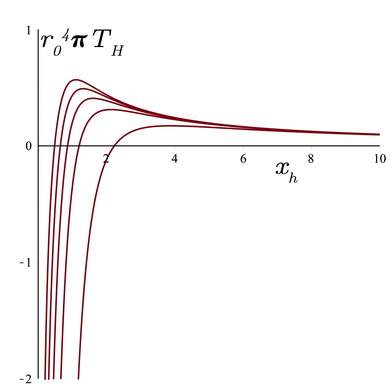
The Hawking temperature is plotted with respect to $x_{h}$ for five different values of $\alpha$ between $0.1$ and $1$ with equal steps. In all plots we have a maximum value for the Hawking temperature where the first derivative is zero.

The Hawking temperature has only one transition point which is type-1. When $x_{h}$ is smaller than the transition point the Hawking temperature is negative and when it is greater than the transition point the Hawking temperature is positive and it tends to zero for $x_{h}\rightarrow\infty$.

Figure 2:

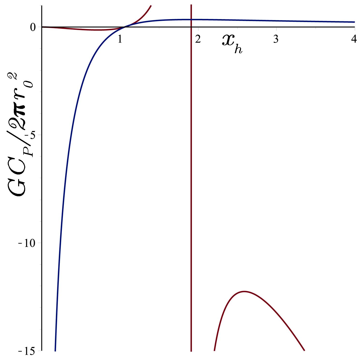
Both the Hawking temperature and heat capacity is plotted for $\alpha=0.5$ in this figure. The heat capacity has two transition points one of which coincides with the transition point of Hawking temperature. The second transition point of the heat capacity is located at a point where the Hawking temperature has its maximum value.

The positivity of heat capacity and Hawking temperature are sign to a physical and stable black hole solutions. The heat capacity has type-1 transition, at which $C_{P}=0$, and type-2 transition, where $C_{P}\rightarrow\infty$, points (the maximum point of Hawking temperature). It is negative when $x_{h}$ is between zero and type-1 transition point and greater than type-2 transition point. It is positive between the transition points, $C_{P}>0$ which is the necessary condition to have thermal stability. As a result the black hole is thermally stable between the transition points where both the heat capacity and Hawking temperature takes positive values.

VI Conclusion:

We have found RN type electric and magnetic black hole solutions in “Double-Logarithmic nonlinear electrodynamics” theory which is given by the Lagrangian (1). The pure magnetic black hole solution is given in terms of elementary functions and becomes singular with a global monopole type constant term which affect the lensing effect by giving rise to an angle of deficiency. In spite of that, the pure electric black hole solution can be expressed as an integral equation. Due to the nice property of magnetic black hole solution we have analyzed its thermodynamic structure. We have derived the black hole first law and the Smarr’s formula. Also, the stability is investigated by use of the heat capacity and Hawking temperature. Both heat capacity and Hawking temperature becomes positive between type-1 and type-2 transition points of heat capacity where the theory turns out to be stable and admits stable black holes.

References

• (1) M. Born, Proc. R. Soc. A 143, 410 (1934).
• (2) M. Born, L. Infeld, Proc. R. Soc. A 144, 425 (1934).
• (3) E. S. Fradkin, A. Tseytlin, Phys. Lett. B 163, 123 (1985).
• (4) A. Tseytlin, Nucl. Phys. B 276, 391 (1986).
• (5) D. M. Gitman, A. E. Shabad, Eur. Phys. J. C 74, 3186 (2014).
• (6) S. I. Kruglov, Eur. Phys. J. C 75, 88 (2015).
• (7) S. I. Kruglov, Ann. Phys. 353, 299 (2015).
• (8) S. I. Kruglov, Ann. Phys. 527, 397 (2015).
• (9) I. Gullu, S. H. Mazharimousavi, arXiv:2009.08665 (2020).
• (10) H. P. de Oliveira, Class Quantum Grav. 11, 1469 (1994).
• (11) W. Heisenberg, H. Euler, Z. Phys. 98, 714 (1936).
• (12) E. Ayon-Beato, A. García, Phys. Rev. Lett. 80, 5056 (1998).
• (13) N. Breton, Phys. Rev. D 67, 124004 (2003).
• (14) I. Dymnikova, Clas. Quant. Grav. 21, 4417 (2004).
• (15) L. Balart, E. C. Vagenas, Phys. Rev. D 90, 124045 (2014).
• (16) S. I. Kruglov, Int. J. Geom. Meth. Mod. Phys. 12, 1550073 (2015).
• (17) H. Reissner, Annalen der Physik, 355, 106-120 (1916).
• (18) G. Nordstrom, Proc. Kon. Ned. Akad. Wet. 20, 1238 (1918).
• (19) S. Fernando, D. Krug, Gen. Relativ. Gravit. 35, 129 (2003).
• (20) T. K. Dey, Phys. Lett. B 595, 484 (2004).
• (21) R.-G. Cai, D.-W. Pang, A. Wang, Phys. Rev. D 70, 124034 (2004).
• (22) D. L. Wiltshire, Phys. Rev. D 38, 2445 (1988).
• (23) M. Aiello, R. Ferraro, G. Giribet, Phys. Rev. D 70, 104014 (2004).
• (24) J. Diaz-Alonso, D. Rubiera-Garcia, Phys. Rev. D 81, 064021 (2010).
• (25) J. Diaz-Alonso, D. Rubiera-Garcia, Phys. Rev. D 82, 085024 (2010).
• (26) J. Diaz-Alonso, D. Rubiera-Garcia, J. Phys. Conf. Ser. 283, 012014 (2011).
• (27) J. Diaz-Alonso, D. Rubiera-Garcia, J. Phys. Conf. Ser. 314, 012065 (2011).
• (28) H. H. Soleng, Phys. Rev. D 52, 6178 (1995).
• (29) H. Yajima, T. Tamaki, Phys. Rev. D 63, 064007 (2001).
• (30) E. Ayon-Beato, A. Garcia, Phys. Lett. B 464, 25 (1999).
• (31) D. J. Cirilo Lombardo, Int. J. Theor. Phys. 48, 2267 (2009).
• (32) A. Burinskii, S. R. Hildebrandt, Phys. Rev. D 65, 104017 (2002).
• (33) M. Novello, S. E. P. Bergliaffa, J. M. Salim, Class. Quantum Grav. 17, 3821 (2000).
• (34) K. A. Bronnikov, Phys. Rev. D 63, 044005 (2001).
• (35) M. Hassaine, C. Martinez, Phys. Rev. D 75, 027502 (2007).
• (36) M. Hassaine, C. Martinez, Class. Quan. Grav. 25, 195023 (2008).
• (37) H. A. Gonzalez, M. Hassaine, C. Martinez, Phys. Rev. D 80, 104008 (2009).
• (38) S. H. Mazharimousavi, M. Halilsoy, O. Gurtug, Class. Quantum Grav. 27, 205022 (2010).
• (39) M. H. Dehghani, H. R. R. Sedehi, Phys. Rev. D 74, 124018 (2006).
• (40) M. H. Dehghani, S. H. Hendi, A. Sheykhi, H. R. Sedehi, J. Cosmol. Astropart. Phys. 02, 020 (2007).
• (41) S. H. Hendi, Phys. Rev. D 82, 064040 (2010).
• (42) [4] S. I. Kruglov, Ann. Phys. 383, 550 (2017).
• (43) S. I. Kruglov, Ann. Phys. 378, 59 (2017).
• (44) S. I. Kruglov, Int. J. Mod. Phys. A 33, 1850023 (2018).
• (45) S. I. Kruglov, Int. J. Mod. Phys. A 32, 1750147 (2017).
• (46) S. I. Kruglov, Ann. Phys. (Berlin) 529, 1700073 (2017).
• (47) S. I. Kruglov, EPL 115, 60006 (2016).
• (48) S. I. Kruglov, Phys. Lett. A 379, 623 (2015).
• (49) R. García-Salcedo, N. Breton, Int. J. Mod. Phys. A 15, 4341 (2000).
• (50) C. S. Camara, M. R. de Garcia Maia, J. C. Carvalho, J. A. S. Lima, Phys. Rev. D 69, 123504 (2004).
• (51) E. Elizalde, J. E. Lidsey, S. Nojiri, S. D. Odintsov, Phys. Lett. B 574, 1 (2003).
• (52) M. Novello, S. E. Perez Bergliaffa, J. M. Salim, Phys. Rev. D 69, 127301 (2004).
• (53) M. Novello, E. Goulart, J. M. Salim, S. E. Perez Bergliaffa, Class. Quant. Grav. 24, 3021 (2007).
• (54) D. N. Vollick, Phys. Rev. D 78, 063524 (2008).
• (55) S. I. Kruglov, Phys. Rev. D 92, 123523 (2015).
• (56) S. I. Kruglov, Int. J. Mod. Phys. D 25, 11, 1640002 (2016).
• (57) L. Labun, J. Rafelski, Phys. Rev. D 81, 065026 (2010).
• (58) R. Schutzhold, Phys. Rev. Lett. 89, 081302 (2002).
• (59) L. Smarr, Phys. Rev. Lett. 30, 71 (1973).
• (60) N. Breton, Gen. Relativ. Gravit. 37, 643 (2005).
• (61) D. A. Rasheed, (1997) arXiv:hep-th/9702087.
• (62) Y. Zhang, S. Gao, Class. Quantum Grav. 35, 145007 (2018).
• (63) S-Q. Hu, X-M. Kuang, Y. C. Ong, Gen. Relativ. Gravit. 51, 55 (2019).
• (64) P. Wang, H. Wu, H. Yang, Eur. Phys. J. C 79, 572 (2019).
• (65) M. Barriola, A. Vilenkin, Phys. Rev. Lett. 63, 341 (1989).
• (66) D. Kastor, S. Ray, J. Traschen, Class. Quantum Grav. 26, 195011 (2009).