Robust Adaptive Control of LPV Systems With
Unmatched Uncertainties

Abstract

In controlling systems with large operating envelopes, it is often necessary to adjust the desired dynamics according to operating conditions. This paper presents a robust adaptive control architecture for linear parameter-varying (LPV) systems that allows for the desired dynamics to be systematically scheduled, while being able to handle a broad class of uncertainties, both matched and unmatched, which can depend on both time and states. The proposed controller adopts an ${\mathcal{L}_{1}}$  adaptive control architecture for designing the adaptive control law and peak-to-peak gain (PPG) minimization for designing the robust control law to mitigate the effect of unmatched uncertainties. Leveraging the PPG bound of an LPV system, we derive transient and steady-state performance bounds in terms of the input and output signals of the actual closed-loop system as compared to the same signals of a nominal system. The efficacy of the proposed method is validated by extensive simulations using the short-period dynamics of an F-16 aircraft operating in a large envelope.

I Introduction

Gain scheduling (GS) is a common practice for controlling nonlinear and time-varying systems with large operating envelopes [1]. As a systematic way for GS design and analysis, the linear parameter-varying (LPV) systems approach has been extensively studied in the last three decades [2, 3, 4, 5], with numerous applications , e.g., in aerospace [6, 7, 8, 9] and automotive systems [10, 11]. On the other hand, model uncertainties and exogenous disturbances are inherent in real-world systems, which lead to degraded stability and performance if not addressed properly. Adaptive control methods have presented a number of promising solutions for controlling uncertain systems under certain assumptions with different guarantees. In the last several decades, the field of adaptive control has witnessed tremendous developments, capturing different classes of linear and nonlinear systems, subject to various parametric and state-dependent uncertainties, and unmodeled dynamics [12, 13, 14]. Despite the significant progress made in the past several decades in model reference adaptive control (MRAC), the solutions are limited to parametric or structured nonlinear uncertainties [12, 14]. Disturbance-observer (DOB) based control and related methods such as active disturbance rejection control (ADRC) [15] are a group of promising approaches for controlling linear and nonlinear systems subject to uncertainties and disturbances [16]. Hereafter, we use DOBC to refer to both DOB based control and the related methods including ADRC. The main idea of DOBC is to lump model uncertainties, unmodeled dynamics, and external disturbances together as a “disturbance”, estimate it via an observation mechanism, and then compute control actions to compensate for the estimated disturbance. However, DOB design often needs inversion of the nominal dynamics (for frequency-domain design methods) which are generally only applicable to minimum-phase LTI systems, or an exogenous system with known parameters that is assumed to generate the disturbances (for time-domain design methods). Moreover, state-dependence of uncertainties are generally ignored in theoretic analysis of DOBC [16]. As an alternative and promising solution for controlling uncertain systems, the ${\mathcal{L}_{1}}$ adaptive control (${\mathcal{L}_{1}}$AC) [17] can handle a broad class of uncertainties without needing a parametric structure, and allows for the use of fast adaptation without sacrificing robustness thanks to the decoupling of the control loop from the estimation loop. Further, ${\mathcal{L}_{1}}$AC provides guaranteed tracking performance, both in transient and steady-state, and guaranteed robustness margins (e.g., nonzero time-delay margin), in the presence of various uncertainties. ${\mathcal{L}_{1}}$AC has been verified on many real-world systems including NASA’s subscale commercial jet [18], and Calspan’s Learjet (a piloted aircraft) [19, 20]. It has also been adopted within the Learn-to-Fly framework of NASA and validated by flight tests [21].

Existing adaptive control and DOBC schemes mostly employ a linear time-invariant (LTI) system to describe the desired or nominal dynamics. However, using an LTI model for a system with a large operating envelope could lead to large uncertainties in certain operating regions. Large uncertainties will cause large compensation actions, which could be energy inefficient or even cause actuator saturation and consequently loss of stability or degraded performance. Additionally, in certain applications, it is preferable to change the desired dynamics according to the operating condition. For instance, for the longitudinal dynamics of manned aircraft, pilots usually prefer faster response at higher speeds and slower response at lower speeds during up-and-away flight [6]. Under these scenarios, using an LPV model to characterize the desired dynamics provides the desired perspective. Nonlinear models have also been employed in adaptive and DOB controllers to describe the desired dynamics [22, 16, 23, 24, 25], but are probably not as appropriate for characterizing the variation of desired dynamics according to operating conditions as an LPV formulation does. Furthermore, for complex systems such as aerospace systems, it may be challenging to get a nonlinear analytic model for the whole operating envelope, e.g., due to the use of look-up tables to model sophisticated aerodynamics. In contrast, it is much easier to obtain an LPV model through interpolation of a series of LTI models resulting from linearization at different operating conditions. However, adaptive or DOB-based control of LPV systems has rarely been explored. [26] studied an MRAC scheme for switched LPV systems, but considered only matched parametric uncertainties with only asymptotic performance guarantees. [27] presented an ${\mathcal{L}_{1}}$AC controller for LPV systems in the presence of matched parametric uncertainties and external disturbances.

It remains a challenging problem in adaptive control or DOBC to handle unmatched uncertainties (UUs), i.e., those that enter the system through different channels from the control inputs. In general, it is impossible to remove the influence of the UUs on system states; therefore, almost all of the existing efforts focus on eliminating or attenuating the effect of UUs on interested variables, e.g., system outputs. For nominal LTI systems that are minimum-phase and square (i.e., having the same number of input and output channels), [28] used the nominal system inversion to design a dynamic feedforward compensation term to remove the effect of the UUs on the output channels in ${\mathcal{L}_{1}}$AC. Similar ideas were explored independently in DOBC, in which static feedforward terms were designed to eliminate the effect of UUs on the outputs in steady state only for LTI systems [29] and nonlinear systems [30]. $H_{\infty}$ control theory was utilized to design state-feedback gains to attenuate the effect of UUs in DOBC [31]. For systems transformable to strict or semi-strict feedback forms, backstepping techniques have been leveraged to handle UUs in adaptive control [32, 33], and in DOBC [34]. Alternative approaches based on learning the UUs and incorporating the learned model to adapt the reference model were investigated in linear MRAC settings [35, 36]. However, the tracking performance during the learning transients can be quite poor, due to a lack of active compensation for the UUs.

Statement of Contributions. The contributions of this paper are threefold. To facilitate systematic scheduling of desired dynamics in controlling uncertain aerospace systems with large operating envelopes, this paper presents a robust adaptive control scheme for LPV systems that can handle a broad class of uncertainties that can depend on both time and states and can be unmatched. The proposed control scheme leverages the ${\mathcal{L}_{1}}$AC architecture to design the adaptive control law. A dynamic feedforward LPV mapping, computed using linear matrix inequality (LMI) techniques, is introduced to attenuate the effect of unmatched uncertainties. This approach is more general and does not need restrictive assumptions such as strict-feedback form, system squareness and non-minimum phase, needed in [32, 33, 34, 28]. As a by-product, we present LMI conditions to synthesize dynamic feedforward LPV controllers for PPG minimization that do not need the derivatives of scheduling parameters for implementation while not relying on structured Lyapunov functions. Second, we derive uniform transient performance bounds in terms of the inputs and states of the robust adaptive system as compared to the same signals of a nominal system. Furthermore, we show that the transient performance bounds can be systematically reduced by reducing the estimation sampling time. Third, we apply the proposed method to control the longitudinal motion of an F-16 aircraft operating in a large envelope, and conduct extensive simulations using both LPV and fully nonlinear models to validate the control performance.

The paper is organized as follows. Section II introduces the main problem and key assumptions. Section III includes basic definitions and preliminary lemmas. Section IV explains the proposed robust adaptive control architecture, while the performance analysis is given in Section V. Section VI includes the simulation results on the short-period dynamics of an F-16 aircraft.

We denote by $\mathbb{R}^{n}$ the set of $n$-dimensional real vectors, $\mathbb{R}^{+}$ the set of non-negative real numbers, $\mathbb{R}^{m\times n}$ the set of real $m$ by $n$ matrices. $\mathbb{I}_{n}$ denotes an $n$ by $n$ identity matrix, and ${0}$ denotes a zero matrix of compatible dimension. $\mathbb{Z}_{i}$ and $\mathbb{Z}_{1}^{n}$ denote the integer sets $\{i,i+1,\cdots\}$ and $\{1,2,\cdots,n\}$, respectively. $\left\lVert\cdot\right\rVert$, $\left\lVert\cdot\right\rVert_{1}$ and $\left\lVert\cdot\right\rVert_{\infty}$ to denote the $2$-norm, $1$-norm and $\infty$-norm of a vector or a matrix, respectively. $\bar{\lambda}(P)$ and $\underline{\lambda}(P)$ denote the maximal and minimal singular values of the matrix $P$, respectively. For symmetric matrices $P$ and $Q$, $P>Q$ means $P-Q$ is positive definite. $\langle X\rangle$ is the shorthand notation of $X+X^{\top\!}$. In symmetric matrices, $\star$ denotes an off-diagonal block induced by symmetry. For a matrix $A\in\mathbb{R}^{m\times n}$, $\mathrm{vec}(A)\in R^{mn}$ represents the vectorization of $A$. The Laplace transform of a function $x(t)$ is denoted by $x(s)\triangleq\mathfrak{L}[x(t)]$. The mapping corresponding to a state-space realization $(A,B,C,D)$ is denoted by ${\left[\begin{array}[]{c|c}A&B\\ \hline\cr C&D\end{array}\right]}$ .

II Problem Statement

Consider the class of multiple-input multiple-output LPV systems subject to uncertainties

$$\dot{x}(t)= ~{}A(\theta(t))x(t)+B(\theta(t))\omega u_{\textup{total}}(t)+f(t,x(t))$$ (1a)

$$y(t)= ~{}C(\theta(t))x(t),\ x(0)=x_{0},$$ (1b)

where $x(t)\in\mathbb{R}^{n}$ is the state vector, $u_{\textup{total}}(t)\in\mathbb{R}^{m}$ is the control input vector, $y(t)\in\mathbb{R}^{p}$ is the output vector, $\theta(t)\triangleq[\theta_{1}(t),\cdots,\theta_{s}(t)]\in\mathbb{R}^{s}$ is a vector of time-varying parameters that can be measured online, $A(\theta(t))\in\mathbb{R}^{n\times n}$, $B(\theta(t))\in\mathbb{R}^{n\times m}$, and $C(\theta(t))\in\mathbb{R}^{m\times n}$ are known matrices dependent on $\theta(t)$. The nominal model $\dot{x}(t)=A(\theta(t))x(t)+B(\theta(t))u_{\textup{total}}(t),y(t)=C(\theta(t))x(t)$ is termed as an LPV model and can be used to characterize a nonlinear system in a large operating envelope [1]. Additionally, $\omega\in\mathbb{R}^{m\times m}$ is an unknown matrix introduced to model actuator failures or modeling errors, which could lead to uncertain control gains or incorrectly estimated control effectiveness [14, Section 9.5]. Moreover, $f\mathrel{\mathop{\mathchar 58\relax}}\mathbb{R}\times\mathbb{R}^{n}\rightarrow\mathbb{R}^{n}$ is an unknown nonlinear function that can represent model uncertainties, unknown parameters and external disturbances [17, Section 2.4]. The initial state vector $x_{0}$ is assumed to be inside an arbitrarily large known set, i.e., for some known $\rho_{0}>0$, $\left\lVert x_{0}\right\rVert\leq\rho_{0}<\infty.$ Hereafter, for the brevity of notation, we often omit the dependence of $\theta(t)$, $x(t)$ and $u(t)$ on $t$. Given 1, we would like to design a controller to ensure stability of the closed-loop system and to track a given bounded piecewise-continuous reference signal $r(t)\in\mathbb{R}^{p}$ (which satisfies $\left\lVert r\right\rVert_{\mathcal{L}_{\infty}}\leq\bar{r}$ for a known constant $\bar{r}$) with prescribed performance.

Assumption 1.

The parameter vector $\theta(t)$ and its derivative are in compact sets, i.e.,

$$\begin{split}\theta(t)\in\Theta,\quad\dot{\theta}(t)\in\Theta_{d},\quad\max_{\dot{\theta}\in\Theta_{d}}\left\lVert\dot{\theta}(t)\right\rVert\leq b_{\dot{\theta}},\end{split}$$ (2)

where $\Theta\triangleq[\underline{\theta}_{1},\bar{\theta}_{1}]\times\cdots\times[\underline{\theta}_{s},\bar{\theta}_{s}]$ and $\Theta_{d}\triangleq[\underline{\nu}_{1},\bar{\nu}_{1}]\times\cdots\times[\underline{\nu}_{s},\bar{\nu}_{s}]$ are known, and $b_{\dot{\theta}}$ is a known constant.

Under Assumption 1, for the nominal or uncertainty-free plant (corresponding to the plant 1 with $\omega=\mathbb{I}_{m}$ and $f(t,x(t))=0$), we can design a baseline controller

$$u_{\textup{bl}}(t)=K_{x}(\theta)x(t),$$ (3)

where $K_{x}(\theta)\in\mathbb{R}^{m\times n}$ is a parameter-dependent (PD) feedback gain matrix to ensure closed-loop stability.

Remark 1.

Assumption 1 is standard in analysis and control synthesis for LPV systems [3, 4, 5, 37, 38], and therefore is not restrictive. In the absence of uncertainties, under Assumption 1, it is straightforward to design the baseline controller 3 using existing methods, e.g., via the PD Lyapunov functions and linear matrix inequalities (LMIs) [4, 3, 5, 38].

With the nominal plant and the baseline controller 3, we can obtain the following ideal (or nominal) closed-loop system

$$\dot{x}_{\textup{id}}(t) =A_{m}(\theta)x_{\textup{id}}(t)+B(\theta)u_{\textup{id}}(t),\ x_{\textup{id}}(0)=x_{0},$$ (4a)

$$u_{\textup{id}}(t) =K_{r}(\theta)x_{\textup{id}}(t),\quad y_{\textup{id}}(t)=C(\theta)x_{\textup{id}}(t),$$ (4b)

where $A_{m}(\theta)\triangleq A(\theta)+B(\theta)K_{x}(\theta)$ and $K_{r}(\theta)\in\mathbb{R}^{m\times p}$ is a parameter-dependent (PD) feedforward gain matrix for achieving desired performance in tracking $r(t)$ in the absence of uncertainties.

Remark 2.

For square systems, i.e., $m=p$, we can set $K_{r}(\theta)=-\left(C(\theta)A_{m}^{-1}(\theta)B(\theta)\right)^{-1}$ to ensure zero steady-state error when tracking a step reference command for any fixed $\theta$ value. For non-square systems, $K_{r}(\theta)$ can be designed using other techniques such as $H_{\infty}$ control.

The goal is to design a state-feedback robust adaptive controller to ensure that $y(t)$ stays close to $y_{\textup{id}}(t)$, the output of the ideal CL system 4, with quantifiable bounds on the transient and steady-state performance. We next introduce the main assumptions needed for theoretical analysis and performance guarantees.

Assumption 2.

(Lyapunov stability of the ideal CL system) There exists a PD symmetric matrix $P(\theta)$ and a positive constant $\mu_{P}$ such that

$$\begin{split}\left\langle\!A_{m}^{\top\!}(\theta)P(\theta)\!\right\rangle+\dot{P}(\theta)&\!\leq\!-\mu_{P}P(\theta),\ \forall(\theta,\dot{\theta})\in\Theta\!\times\!\Theta_{d},\\ P(\theta)&\!>\!0,\ \forall\theta\in\Theta.\end{split}$$ (5)

Remark 3.

Assumption 2 ensures stability of 4 [3]. Indeed, given the closed-loop system 4a, the matrix $P(\theta)$ that satisfies 5 (which defines a PD Lyapunov function $V(t,\theta)\triangleq x^{\top\!}(t)P(\theta)x(t)$) can be easily searched for via solving a parameter-dependent LMI (PD-LMI) problem [38, 3, Section 1.3]. Moreover, the matrix $P(\theta)$ that satisfies 5 is automatically generated if the baseline controller is designed using PD Lyapunov functions [3, 4] (see also the example in Section VI-A). Therefore, Assumption 2 is not restrictive.

Given the baseline controller in 3, we adopt a compositional control law in the form of

$$u_{\textup{total}}(t)=u_{\textup{bl}}(t)+u(t),$$ (6)

where $u(t)$ is a robust adaptive control law to be designed to compensate for the uncertainties and track the reference signal $r(t)$.

Assumption 3.

(Partial knowledge of input gain) The input gain matrix $\omega$ is assumed to be an unknown strictly row-diagonally dominant matrix with $\textup{sgn}(\omega_{ii})$ known. Furthermore, we assume that $\omega\in\Omega\triangleq\{\omega\in\mathbb{R}^{m\times m}\mathrel{\mathop{\mathchar 58\relax}}\mathrm{vec}(w)\in\hat{\Omega}\}$ with $\hat{\Omega}\subset\mathbb{R}^{m^{2}}$ being a convex polytope. Without loss of generality, we further assume that $\mathbb{I}_{m}\in\Omega$.

Remark 4.

The first statement in Assumption 3 indicates that $\omega$ is always non-singular with known sign for the diagonal elements, and is essentially the same as the assumptions made in existing relevant work in adaptive control, e.g, [39] [12, Sections 6 and 7]. The choice of the form for $\omega$ is motivated by aerospace applications where control directions are known but their magnitudes and coupling are uncertain [39].

Assumption 4.

(Uniform boundedness of $f(t,0)$) There exist constants $b_{f}^{0}$ such that $\left\lVert f(t,0)\right\rVert\leq b_{f}^{0}$, for any $t\geq 0$.

Assumption 5.

(Semiglobal Lipschitz continuity of $f(t,x)$) For arbitrary $\delta>0$, there exist positive constants $L_{f}^{\delta}$ such that $\left\lVert f(t,x_{1})-f(t,x_{2})\right\rVert\leq L_{f}^{\delta}\left\lVert x_{1}-x_{2}\right\rVert,$ for any $t\geq 0$ and any $x_{j}$ satisfying $\left\lVert x_{j}\right\rVert\leq\delta,\ j=1,2$.

Assumption 6.

(Uniform boundedness of rate of variation of $f(t,x)$ with respect to $t$) There exists positive constant $l_{f}$ such that for any $x$ and $t_{1},t_{2}\geq 0$, $\left\|{f(t_{1},x)-f(t_{2},x)}\right\|\leq{l_{f}}\left\lvert t_{1}-t_{2}\right\rvert.$

Remark 5.

Roughly speaking, Assumptions 5 and 6 require the rate of variation of $f(t,x)$ with respect to both $x$ and $t$ to be bounded, which are less restrictive than requiring the uncertainties to be slowly varying (i.e., $\dot{f}\simeq 0$) [30] or have constant values in steady state (i.e., $\lim_{t\rightarrow\infty}\dot{f}=0$) [29, 34] needed in some DOBC work.

Assumption 7.

$B(\theta)$ has full column rank for all $\theta\in\Theta$, and there exist positive constants $L_{B}$, $L_{B^{\dagger}}$ and $L_{K_{x}}$ such that

$$\left\lVert B(\theta^{1})-B(\theta^{2})\right\rVert \leq L_{B}\left\lVert\theta^{1}-\theta^{2}\right\rVert,$$ (7)

$${\left\lVert B^{\dagger}(\theta^{1})-B^{\dagger}(\theta^{2})\right\rVert} {\leq L_{B^{\dagger}}\left\lVert\theta^{1}-\theta^{2}\right\rVert},$$ (8)

$${\left\lVert K_{x}(\theta^{1})-K_{x}(\theta^{2})\right\rVert} {\leq L_{K_{x}}\left\lVert\theta^{1}-\theta^{2}\right\rVert,}$$ (9)

for any $\theta^{i}\in\Theta$, $i=1,2$, where $B^{\dagger}(\theta)$ denotes the pseudo-inverse of $B(\theta)$, and $K_{x}(\theta)$ is the gain of the baseline controller 3.

III Preliminaries and Basic Lemmas

In this section, we introduce some definitions, notations, and lemmas for deriving the main results. Hereafter, for notation compactness, we often omit the time dependence of $\theta$ and $x$.

Under Assumption 7, let us define

$$\bar{B}(\theta)\triangleq\left[B(\theta),B_{u}(\theta)\right],$$ (10)

where $B_{u}(\theta)\in\mathbb{R}^{n\times(n-m)}$ is a matrix dependent on $\theta$ such that $\textup{rank}[\bar{B}(\theta)]=n$ and $B^{\top\!}(\theta)B_{u}(\theta)=0$ for any $\theta\in\Theta$. On the other hand, since $\textup{rank}[\bar{B}(\theta)]=n$ and $B^{\top\!}(\theta)B_{u}(\theta))=0$ for any $\theta\in\Theta$, we can always find vector-valued functions $f_{i}(t,x(t))$ ($i=1,2$) such that

$$\bar{B}(\theta)[f_{1}^{\top\!}(t,x),f_{2}^{\top\!}(t,x)]^{\top\!}=B(\theta)f_{1}(t,x)+B_{u}(\theta)f_{2}(t,x)=\!{\bar{f}}(t,x)\!\triangleq\!f(t,x)\!+\!B(\theta)(\omega\!-\!\mathbb{I}_{m})K_{x}(\theta)x\!$$ (11)

holds for any $t$ and any $\theta\in\Theta$, where the dependence of $x(t)$ and $r(t)$ on $t$ has been omitted for brevity. With 6, 3 and 11, the system (1) can be rewritten as

$$\dot{x}(t)\!= ~{}A_{m}(\theta)x(t)\!+\!B(\theta)\omega u(t)\!+\!{\bar{f}}(t,x(t))$$ (12a)

$$\!= ~{}A_{m}(\theta)x(t)\!+\!B(\theta)\left(\omega u(t)\!+\!f_{1}(t,x(t))\right)+\!B_{u}(\theta)f_{2}(t,x(t)),$$ (12b)

$$y(t)\!= ~{}C(\theta)x(t),\ x(0)=x_{0}.$$ (12c)

Since the set $\Theta$ (introduced in Assumption 1) and the parameter-dependent matrices are all known, we can define and compute the following constants:

$$b_{A_{m}}\!\!\triangleq\!\max_{\theta\in\Theta}\!\left\lVert A_{m}(\theta)\right\rVert,\ b_{B}\!\triangleq\!\max_{\theta\in\Theta}\!\left\lVert B(\theta)\right\rVert,\ b_{B^{\dagger}}\!\triangleq\!\max_{\theta\in\Theta}\!\left\lVert B^{\dagger}(\theta)\right\rVert,$$

$$b_{C}\!\triangleq\!\max_{\theta\in\Theta}\!\left\lVert C(\theta)\right\rVert,\ b_{B_{u}}\!\triangleq\!\max_{\theta\in\Theta}\!\left\lVert B_{u}(\theta)\right\rVert,\ b_{B_{u}^{\dagger}}\!\triangleq\!\max_{\theta\in\Theta}\!\left\lVert B_{u}^{\dagger}(\theta)\right\rVert,$$

$${b_{K_{x}}\!\triangleq\!\max_{\theta\in\Theta}\!\left\lVert K_{x}(\theta)\right\rVert,\ b_{K_{r}}\!\triangleq\!\max_{\theta\in\Theta}\!\left\lVert K_{r}(\theta)\right\rVert},$$ (13)

where $B_{u}^{\dagger}(\theta)$ denotes the pseudo-inverse of $B_{u}(\theta)$ introduced in 10. Next, we present a lemma stating some properties of $f_{i}(t,x)$ under the assumptions introduced in Section II. The proof is given in Appendix A-A.

Lemma 1.

Suppose Assumptions 3, 1, 7, 4, 5 and 6 hold, and consider the functions ${\bar{f}}(t,x)$ and $f_{i}(t,x)$ ($i=1,2$) that satisfy 11. Then, given an arbitrary $\delta>0$, for any $x_{i}$ satisfying $\left\lVert x_{i}\right\rVert\leq\delta$ ($i=1,2$) and for any $t_{i}\geq 0$ ($i=1,2$), we have

$$\left\lVert{\bar{f}}(t,0)\right\rVert \leq b_{f}^{0},\ \forall t\geq 0,$$ (14)

$$\left\|{f_{i}(t,0)}\right\| \leq{b_{f_{i}}^{0}},\ \forall t\geq 0,$$ (15)

$$\left\|{{\bar{f}}(t_{1},x_{1})\!-\!{\bar{f}}(t_{2},x_{2})}\right\| \leq{L_{{\bar{f}}}^{\delta}}\left\|{x_{1}\!-\!x_{2}}\right\|+l_{\bar{f}}\left\lvert t_{1}\!-\!t_{2}\right\rvert,$$ (16)

$$\left\|{f_{i}(t_{1},x_{1})\!-\!f_{i}(t_{2},x_{2})}\right\| \leq{L_{f_{i}}^{\delta}}\left\|{x_{1}\!-\!x_{2}}\right\|+l_{f_{i}}\left\lvert t_{1}\!-\!t_{2}\right\rvert,$$ (17)

where $b_{f}^{0}$ is introduced in Assumption 4, and

$$b_{f_{1}}^{0}\! \triangleq b_{B^{\dagger}}b_{f}^{0},b_{f_{2}}^{0}\triangleq b_{B^{\dagger}_{u}}b_{f}^{0},$$ (18a)

$$l_{\bar{f}} \triangleq{l_{f}}+{\max\limits_{\omega\in\Omega}}\left\|{\omega-{\mathbb{I}_{m}}}\right\|\left({L_{B}b_{K_{x}}+b_{B}{L_{K_{x}}}}\right)\delta{b_{\dot{\theta}}},$$ (18b)

$$L_{\bar{f}} \triangleq{L_{f}^{\delta}}+\mathop{\max}\limits_{\theta\in\Theta}\left\|{B(\theta)K_{x}(\theta)}\right\|{\max\limits_{\omega\in\Omega}}\left\|{\omega-{\mathbb{I}_{m}}}\right\|,$$ (18c)

$$l_{f_{1}}\! \triangleq{l_{f}}b_{B^{\dagger}}\!+\!L_{B^{\dagger}}b_{\dot{\theta}}({b_{f}^{0}}\!+\!{L_{f}^{\delta}}\delta)\!+\!{L_{K_{x}}}b_{\dot{\theta}}\delta{\max_{\omega\in\Omega}}\left\|{\omega\!-\!{\mathbb{I}_{m}}}\right\|,$$ (18d)

$$l_{f_{2}}\! \triangleq{l_{f}}b_{B_{u}^{\dagger}}+L_{B_{u}^{\dagger}}b_{\dot{\theta}}({b_{f}^{0}}+{L_{f}^{\delta}}\delta),$$ (18e)

$$L_{f_{1}}^{\delta}\! \triangleq{L_{f}^{\delta}}b_{B^{\dagger}}\!+\!\!{\max\limits_{\omega\in\Omega,\>\theta\in\Theta}}\left\|{(\omega\!-\!{\mathbb{I}_{m}})K_{x}(\theta)}\right\|,$$ (18f)

$$L_{f_{2}}^{\delta}\! \triangleq{L_{f}^{\delta}}b_{B_{u}^{\dagger}}.$$ (18g)

Definition 1.

The $\mathcal{L}_{\infty}$ and truncated $\mathcal{L}_{\infty}$ norm of a function $x\mathrel{\mathop{\mathchar 58\relax}}\mathbb{R}^{+}\rightarrow\mathbb{R}^{n}$ are defined as $\left\lVert x\right\rVert_{\mathcal{L}_{\infty}}\triangleq\sup_{t\geq 0}\left\lVert x(t)\right\rVert$, and $\left\lVert x\right\rVert_{\mathcal{L}_{\infty}^{[0,\tau]}}\triangleq\sup_{0\leq t\leq\tau}\left\lVert x(t)\right\rVert$, respectively.

Definition 2.

[40, Section III.F] For a stable proper MIMO system $H(s)$ with input $\mathrm{u}(t)\in\mathbb{R}^{m}$ and output $\mathrm{y}(t)\in\mathbb{R}^{p}$, its ${\mathcal{L}_{1}}$ norm is defined as

$$\left\lVert H(s)\right\rVert_{\mathcal{L}_{1}}\triangleq\sup_{\mathrm{x}(0)=0,\left\lVert\mathrm{u}\right\rVert_{\mathcal{L}_{\infty}}\leq 1}{\left\lVert\mathrm{y}\right\rVert_{\mathcal{L}_{\infty}}}.$$ (19)

The ${\mathcal{L}_{1}}$ norm of an LTI system in Definition 2 is also known as the peak-to-peak gain (PPG) [40, Section III.F]. The following lemma is directly from Definition 2.

Lemma 2.

For a stable proper MIMO system $H(s)$ with input $\mathrm{u}(t)\in\mathbb{R}^{m}$ and output $\mathrm{y}(t)\in\mathbb{R}^{p}$, we have $\left\lVert\mathrm{y}\right\rVert_{\mathcal{L}_{\infty}^{[0,\tau]}}\leq\left\lVert H(s)\right\rVert_{\mathcal{L}_{1}}\left\lVert\mathrm{u}\right\rVert_{\mathcal{L}_{\infty}^{[0,\tau]}}$, for any $\tau\geq 0$.

Remark 6.

We use the vector 2-norm in definition of the ${\mathcal{L}_{\infty}}$ function norm (Definition 1) to further define the ${\mathcal{L}_{1}}$ system norm (Definition 2), which is different from the common practice that uses the vector $\infty$-norm (see e.g., [17, Section A.7.1]).

Let $x_{\textup{in}}$ be the state of the system

$$\dot{x}_{\textup{in}}(t)=A_{m}(\theta)x_{\textup{in}}(t),\quad x_{\textup{in}}(0)=x_{0}.$$ (20)

Then $x_{\textup{in}}$ is bounded according to the following lemma.

Lemma 3.

Given the autonomous system in (20), under Assumption 2, the following inequality holds:

$$\left\lVert x_{\textup{in}}\right\rVert_{\mathcal{L}_{\infty}}\leq\rho_{\textup{in}},$$ (21)

where $\rho_{\textup{in}}\triangleq\rho_{0}\sqrt{\frac{{\max_{\theta\in\Theta}{\bar{\lambda}(P(\theta))}}}{{\min_{\theta\in\Theta}{\underline{\lambda}(P(\theta))}}}}$ with $\rho_{0}$ defined below (1).

Proof. Define $V(t,\theta)\triangleq x_{\textup{in}}^{\top\!}(t)P(\theta)x_{\textup{in}}(t)$, where $P(\theta)$ is introduced in (5). From the dynamics in (20) and the inequality in (5), we have

$$\dot{V}(t,\theta) =x_{\textup{in}}^{\top\!}(t)\left(A_{m}^{\top\!}(\theta)P(\theta)+P(\theta)A_{m}(\theta)+\dot{P}(\theta)\right)x_{\textup{in}}(t)\leq-\mu_{P}x_{\textup{in}}^{\top\!}(t)P(\theta)x_{\textup{in}}(t)=-\mu_{P}V(t,\theta).$$

Therefore, $V(t,\theta)\leq V(0,\theta(0))\textup{e}^{-\mu_{P}t}\leq x_{\textup{in}}^{\top\!}(0)P(\theta(0))x_{\textup{in}}(0)\textup{e}^{-\mu_{P}t}\leq{\max_{\theta\in\Theta}{\bar{\lambda}(P(\theta))}}\left\lVert x_{0}\right\rVert^{2}\textup{e}^{-\mu_{P}t}.$ The preceding inequality, together with the fact that $V(t,\theta)\geq{\min_{\theta\in\Theta}{\underline{\lambda}(P(\theta))}}\left\lVert x_{\textup{in}}(t)\right\rVert^{2},$ leads to

$$\begin{split}\left\lVert x_{\textup{in}}(t)\right\rVert&\leq\left\lVert x_{0}\right\rVert\sqrt{\frac{{\max_{\theta\in\Theta}{\bar{\lambda}(P(\theta))}}}{{\min_{\theta\in\Theta}{\underline{\lambda}(P(\theta))}}}}\textup{e}^{-\frac{\mu_{P}}{2}t}\leq\rho_{0}\sqrt{\frac{{\max_{\theta\in\Theta}{\bar{\lambda}(P(\theta))}}}{{\min_{\theta\in\Theta}{\underline{\lambda}(P(\theta))}}}},\quad\forall t\geq 0,\end{split}$$

which proves (21). $\blacksquare$

We next consider a general LPV system:

$$\mathcal{G}(\theta)\mathrel{\mathop{\mathchar 58\relax}}\left\{\begin{aligned} \dot{\mathrm{x}}(t)&=\mathrm{A}(\theta(t))\mathrm{x}(t)+\mathrm{B}(\theta(t))\mathrm{u}(t),\\ \mathrm{y}(t)&=\mathrm{C}(\theta(t))\mathrm{x}(t)+\mathrm{D}(\theta(t))\mathrm{u}(t),\end{aligned}\right.$$ (22)

where $\mathrm{x}(t)\in\mathbb{R}^{n},\ \mathrm{u}(t)\in\mathbb{R}^{m},\ \mathrm{y}(t)\in\mathbb{R}^{p}$, and $\mathrm{A}(\theta),\mathrm{B}(\theta),\mathrm{C}(\theta),\mathrm{D}(\theta)$ are state-space matrices of compatible dimensions depending on the varying parameter vector $\theta(t)\in\mathbb{R}^{s}$. Furthermore, the trajectory of $\theta$ is constrained by (2). We use $\mathcal{G}(\theta)$ to denote the input-output mapping of the system in (22).

Definition 3 ([41]).

Given a stable LPV system in (22) subject to Assumption 1, the PPG of $\mathcal{G}(\theta)$ is defined as

$$\left\lVert\mathcal{G}(\theta)\right\rVert_{\mathcal{L}_{1}}\triangleq\sup_{\mathrm{x}(0)=0,\ \left\lVert\mathrm{u}\right\rVert_{\mathcal{L}_{\infty}}\leq 1}\sup_{\ \theta(t)\in\Theta,\ \dot{\theta}(t)\in\Theta_{d}}{\left\lVert\mathrm{y}\right\rVert_{\mathcal{L}_{\infty}}}.$$ (23)

Moreover, a positive scalar $\gamma$ is a bound on the PPG of $\mathcal{G}(\theta)$ if for $\mathrm{x}(0)=0$ and all trajectories of $\theta$ satisfying (2), we have

$$\left\lVert\mathrm{y}\right\rVert_{\mathcal{L}_{\infty}^{[0,\tau]}}\leq\gamma\left\lVert\mathrm{u}\right\rVert_{\mathcal{L}_{\infty}^{[0,\tau]}},\quad\forall\tau\geq 0.$$ (24)

The PPG is equivalent to the ${\mathcal{L}_{1}}$ norm for an LTI system, and thus we still use $\left\lVert\cdot\right\rVert_{\mathcal{L}_{1}}$ to denote the PPG of an LPV system. In practice, it is very challenging to compute the PPG of an LPV system exactly. However, a PPG bound can be computed using LMI techniques (see Lemma 5). Hereafter, we use $\left\lVert\mathcal{G}(\theta)\right\rVert_{\bar{\mathcal{L}}_{1}}$ to denote an arbitrary PPG bound of $\mathcal{G}(\theta)$. Next lemma follows straightforwardly from the inequalities in (23) and (24), and thus the proof is omitted.

Lemma 4.

Given a stable LPV system in (22) with $\mathrm{x}(0)=0$, we have

$$\left\lVert\mathrm{y}\right\rVert_{\mathcal{L}_{\infty}^{[0,\tau]}}\leq\left\lVert\mathcal{G}(\theta)\right\rVert_{\bar{\mathcal{L}}_{1}}\left\lVert\mathrm{u}\right\rVert_{\mathcal{L}_{\infty}^{[0,\tau]}},\quad\forall\tau\geq 0.$$ (25)

The LMI conditions for computing a PPG bound for an LTI system are given in [40, Section III.F]. The following lemma is a straightforward extension of this result to LPV systems using the PD Lyapunov function $V(t,\theta)=\mathrm{x}^{\top\!}(t)\mathrm{P}(\theta)\mathrm{x}(t)$. Therefore, the detailed proof is omitted for brevity.

Lemma 5.

Given the LPV system in (22) subject to Assumption 1, it is bounded-input-bounded-output (BIBO) stable, and $\gamma>0$ is a PPG bound of this system, if there exist a PD and symmetric matrix $\mathrm{P}(\theta)$ and positive constants $\mu$ and $\upsilon$, such that the following inequalities hold:

$$\begin{bmatrix}[1.2]\left\langle\mathrm{A}^{\top\!}(\theta)\mathrm{P}(\theta)\right\rangle+\mu\mathrm{P}(\theta)+\dot{\mathrm{P}}(\theta)&\star\\ \mathrm{B}^{\top\!}(\theta)\mathrm{P}(\theta)&-\upsilon\mathbb{I}_{m}\end{bmatrix}<0,\quad\forall(\theta,\dot{\theta})\in\Theta\times\Theta_{d},$$ (26)

$$\begin{bmatrix}[1]\mu\mathrm{P}(\theta)&\star&\star\\ 0&(\gamma-\upsilon)\mathbb{I}_{m}&\star\\ \mathrm{C}(\theta)&\mathrm{D}(\theta)&\gamma\mathbb{I}_{p}\end{bmatrix}>0,\quad\forall\theta\in\Theta.$$ (27)

Remark 7.

Due to the term $\mu\mathrm{P}(\theta)$, the inequalities (26) and (27) are only LMIs if $\mu$ is fixed. Thus, finding the best bound requires performing a line search over $\mu>0$. The PD-LMIs 26 and 27, despite involving the derivatives of decision matrices, are standard in the LPV literature [4], and can be readily solved by available techniques (see Section IV-C).

The following lemma characterizes the state evolution of a BIBO stable LPV system, given a bounded input.

Lemma 6.

Consider an LPV system in (22) with $\mathrm{x}(0)=0$, subject to Assumption 1. If there exists a PD symmetric matrix $\mathrm{P}(\theta)$ and a constant $\mu>0$ such that

$$\left\langle\mathrm{A}^{\top\!}(\theta)\mathrm{P}(\theta)\right\rangle+\dot{\mathrm{P}}(\theta)\leq-\mu\mathrm{P}(\theta),\ \forall(\theta,\dot{\theta})\in\Theta\times\Theta_{d},$$ (28)

then

$$\left\lVert\mathrm{x}(t)\right\rVert\leq\beta_{\Theta}(t,\mu,\mathrm{P}(\theta),\mathrm{B}(\theta))\left\lVert\mathrm{u}\right\rVert_{\mathcal{L}_{\infty}^{[0,t]}},\quad\forall t\geq 0,$$ (29)

where

$$\!\!\!\beta_{\Theta} (t,\mu,\mathrm{P},\mathrm{B})\!\triangleq\!\sqrt{\!\sqrt{\frac{\lambda_{2}}{\lambda_{1}}}(1\!-\!e^{-\mu t})}\frac{2}{\mu\lambda_{1}}\!\max_{\theta\in\Theta}\!\left\lVert\mathrm{P}(\theta)\mathrm{B}(\theta)\right\rVert\!,$$ (30)

$$\!\!\!\lambda_{1} ={\min_{\theta\in\Theta}{\underline{\lambda}(\mathrm{P}(\theta))}},\ \lambda_{2}={\max_{\theta\in\Theta}{\bar{\lambda}(\mathrm{P}(\theta))}}.$$ (31)

Proof. Define $V(t,\theta)=\mathrm{x}^{\top\!}(t)\mathrm{P}(\theta)\mathrm{x}(t)$. Then,

$$\dot{V}(t,\theta) =\mathrm{x}^{\top\!}\left(\langle\mathrm{A}^{\top\!}(\theta)\mathrm{P}(\theta)\rangle+\dot{\mathrm{P}}(\theta)\right)\mathrm{x}+2\mathrm{x}^{\top\!}\mathrm{P}(\theta)\mathrm{B}(\theta)u\leq-\mu\mathrm{x}^{\top\!}\mathrm{P}(\theta)\mathrm{x}+2\mathrm{x}^{\top\!}\mathrm{P}(\theta)\mathrm{B}(\theta)\mathrm{u}$$ (32)

$$\leq-\mu\lambda_{1}\left\lVert\mathrm{x}(t)\right\rVert^{2}+2\left\lVert\mathrm{x}(t)\right\rVert\left\lVert\mathrm{P}(\theta)\mathrm{B}(\theta)\right\rVert\left\lVert\mathrm{u}(t)\right\rVert\leq 0,\quad\forall\left\lVert\mathrm{x}(t)\right\rVert\geq\frac{2}{\mu\lambda_{1}}\max_{\theta\in\Theta}\left\lVert\mathrm{P}(\theta)\mathrm{B}(\theta)\right\rVert\left\lVert\mathrm{u}\right\rVert_{\mathcal{L}_{\infty}^{[0,t]}}.$$

The preceding inequality indicates that

$$V(t,\theta)\leq\lambda_{2}\left(\frac{2}{\mu\lambda_{1}}\max_{\theta\in\Theta}\left\lVert\mathrm{P}(\theta)\mathrm{B}(\theta)\right\rVert\left\lVert\mathrm{u}\right\rVert_{\mathcal{L}_{\infty}^{[0,t]}}\right)^{2},$$ (33)

which, together with $V(t,\theta)\geq\lambda_{1}\left\lVert\mathrm{x}(t)\right\rVert^{2}$, implies that

$$\left\lVert\mathrm{x}\right\rVert_{\mathcal{L}_{\infty}^{[0,t]}}\leq\sqrt{\frac{\lambda_{2}}{\lambda_{1}}}\frac{2}{\mu\lambda_{1}}\max_{\theta\in\Theta}\left\lVert\mathrm{P}(\theta)\mathrm{B}(\theta)\right\rVert\left\lVert\mathrm{u}\right\rVert_{\mathcal{L}_{\infty}^{[0,t]}}.$$ (34)

Next, we show that the preceding bound on $\mathrm{x}$ can be further improved. Equation (32) indicates that

$$\dot{V}(t,\theta)\leq-\mu V(t,\theta)+2\left\lVert\mathrm{x}(t)\right\rVert\left\lVert\mathrm{P}(\theta)\mathrm{B}(\theta)\right\rVert\left\lVert\mathrm{u}(t)\right\rVert,$$

which, together with $V(0,\theta)=0$, leads to

$$V(t,\theta)\leq e^{-\mu t}V(0,\theta)+\int_{0}^{t}e^{-\mu(t-\tau)}2\left\lVert\mathrm{x}(\tau)\right\rVert\left\lVert\mathrm{P}(\theta(\tau))\mathrm{B}(\theta(\tau))\right\rVert\left\lVert\mathrm{u}(\tau)\right\rVert d\tau$$

$$\leq 2\left\lVert\mathrm{x}\right\rVert_{\mathcal{L}_{\infty}^{[0,t]}}\max_{\theta\in\Theta}\left\lVert\mathrm{P}(\theta)\mathrm{B}(\theta)\right\rVert\left\lVert\mathrm{u}\right\rVert_{\mathcal{L}_{\infty}^{[0,t]}}\int_{0}^{t}e^{-\mu(t-\tau)}d\tau$$

$$\leq 2\left\lVert\mathrm{x}\right\rVert_{\mathcal{L}_{\infty}^{[0,t]}}\max_{\theta\in\Theta}\left\lVert\mathrm{P}(\theta)\mathrm{B}(\theta)\right\rVert\left\lVert\mathrm{u}\right\rVert_{\mathcal{L}_{\infty}^{[0,t]}}\frac{1}{\mu}(1-e^{-\mu t}).$$

By plugging (34) into the above equality and further considering $V(t,\theta)\geq\lambda_{1}\left\lVert\mathrm{x}(t)\right\rVert^{2}$, we arrive at (29). $\blacksquare$

The following lemma refines the result in Lemma 6 and establishes individual bounds for the states of (22) before and after an arbitrary time instant $T$.

Lemma 7.

Given an LPV system in (22) with $\mathrm{x}(0)=0$, subject to Assumption 1, assuming that there exists a PD and symmetric matrix $\mathrm{P}(\theta)$ and a constant $\mu>0$ such that (28) holds, we have

$$\left\lVert\mathrm{x}(t)\right\rVert\leq\!\left\{\!\!\!\begin{array}[]{lr}\beta_{\Theta}(T,\mu,\mathrm{P},\mathrm{B})\left\lVert\mathrm{u}\right\rVert_{\mathcal{L}_{\infty}^{[0,T]}},\ \forall 0\leq t\leq T,\\ \!\!\!\begin{array}[]{l}\sqrt{\frac{\lambda_{2}}{\lambda_{1}}}\beta_{\Theta}(T,\mu,\mathrm{P},\mathrm{B})\left\lVert\mathrm{u}\right\rVert_{\mathcal{L}_{\infty}^{[0,T]}}\,\negmedspace{}+\beta_{\Theta}(\infty,\mu,\mathrm{P},\mathrm{B})\left\lVert\mathrm{u}\right\rVert_{\mathcal{L}_{\infty}^{[T,t]}},\ \forall t>T,\end{array}\end{array}\right.$$ (35)

where $\lambda_{i}$ ($i=1,2$) are defined in (31).

Proof. The first part follows directly from Lemma 6, along with the fact that for $0\leq t\leq T$, $\beta_{\Theta}(t,\mu,\mathrm{P},\mathrm{B})$ $\leq\beta_{\Theta}(T,\mu,\mathrm{P},\mathrm{B})$. The second part results from application of Lemmas 3 and 6 considering the state evolution starting from $T$ with the initial condition $x(T)$ , as well as the fact of $\beta_{\Theta}(t-T,\mu,\mathrm{P},\mathrm{B})\leq\beta_{\Theta}(\infty,\mu,\mathrm{P},\mathrm{B})$ for any $t>T$. $\blacksquare$

IV Robust Adaptive Control of LPV Systems With Unmatched Uncertainties

A unique feature of an $\mathcal{L}_{1}$AC architecture is a low-pass filter that decouples the estimation loop from the control loop, thereby allowing for arbitrarily fast adaptation without sacrificing the robustness [17]. In the presence of unknown input gain as considered in this paper, the filter is constructed through a feedback gain matrix $K\in\mathbb{R}^{m\times m}$ and an $m\times m$ strictly proper transfer function matrix $D(s)$, which lead, for all $\omega\in\Omega$, to a strictly proper stable low-pass filter $\mathcal{C}(s)\triangleq\omega KD(s)(\mathbb{I}_{m}+\omega KD(s))^{-1},$ with DC gain $C(0)=\mathbb{I}_{m}$. The gain $K$ and the filter $D(s)$ will be used in the control law in (46). See also Remark 9 for more insights. For simplifying the derivations, we set $D(s)=\frac{1}{s}\mathbb{I}_{m}$, which leads to

$$\mathcal{C}(s)=\omega K(s\mathbb{I}_{m}+\omega K)^{-1}.$$ (36)

Hereafter, we use the notation $\mathcal{C}$ (i.e., without argument) to denote the input-output mapping corresponding to the transfer function matrix $\mathcal{C}(s)$. We now introduce a few notations to be used later in the controller design and performance analysis. Let $\mathcal{H}_{xm}(\theta)$ and $\mathcal{H}_{m}(\theta)$ respectively denote the input-to-state and input-to-output mappingsof the system

$$\dot{x}(t)=A_{m}(\theta)x(t)+B(\theta)u(t),\ y(t)=C(\theta)x(t),$$ (37)

and $\mathcal{H}_{xum}(\theta)$ and $\mathcal{H}_{um}(\theta)$ respectively denote the input-to-state and input-to-output mappings of the system

$$\dot{x}(t)=A_{m}(\theta)x(t)+B_{u}(\theta)u(t),\ y(t)=C(\theta)x(t).$$ (38)

We further define

$$\mathcal{G}_{xm}(\theta) \triangleq\mathcal{H}_{xm}(\theta)(\mathbb{I}_{m}-\mathcal{C}),$$ (39a)

$$\mathcal{G}_{xum}(\theta) \triangleq\mathcal{H}_{xum}(\theta)-\mathcal{H}_{xm}(\theta)\mathcal{C}{\bar{\mathcal{H}}}(\theta).$$ (39b)

In (39b), ${\bar{\mathcal{H}}}(\theta)$ is a $\theta$-dependent mapping designed to mitigate the effect of the unmatched uncertainty, detailed in Section IV-B. For presentation of Section IV-B, we also define

$$\mathcal{G}_{m}(\theta)\triangleq C(\theta)\mathcal{G}_{xm}(\theta),\ \mathcal{G}_{um}(\theta)\triangleq C(\theta)\mathcal{G}_{xum}(\theta),$$ (40)

where $C(\theta)$ is the output matrix in (1).

IV-A Proposed control architecture

The dynamics in 12a is equivalent to

$$\dot{x}(t)=A_{m}(\theta)x(t)+B(\theta)u(t)+\sigma(t,x(t),u(t)),$$ (41)

where

$$\sigma(t,x(t),u(t))\triangleq B(\theta)(\omega-\mathbb{I}_{m})u(t)+{\bar{f}}(t,x(t)),$$ (42)

with ${\bar{f}}(t,x(t))$ defined in 11. We now describe the proposed robust adaptive control architecture (see Fig. 1) consisting of a state predictor, an adaptive law and a low-pass filtered control law.

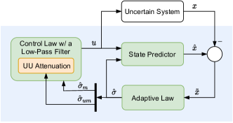
Figure 1: Proposed robust adaptive control architecture

State Predictor: The state predictor is selected as:

$$\begin{split}\dot{\hat{x}}(t)&=A_{m}(\theta)x(t)+B(\theta)u(t)+\hat{\sigma}(t)-a\tilde{x}(t),\end{split}$$ (43)

where $\hat{x}(0)={x}_{0}$, $\hat{x}(t)\in\mathbb{R}^{n}$ is the predicted state vector, $\tilde{x}(t)\triangleq\hat{x}(t)-x(t)$ is the prediction error, $a$ is a positive scalar, and $\hat{\sigma}(t)$ is the adaptive estimation of the lumped uncertainty, $\sigma(t,x,u)$, defined in 42.

Adaptive Law: The estimation $\hat{\sigma}(t)$ is updated by the following piecewise-constant estimation law (similar to that in [17, Section 3.3]):

$$\begin{split}\hat{\sigma}(t)&=\hat{\sigma}(iT),\quad t\in[iT,(i+1)T),\\ \hat{\sigma}(iT)&=-\Upsilon(T)\tilde{x}(iT),\end{split}$$ (44)

for $i=0,1,\cdots$, where $T$ is the estimation sampling time, and $\Upsilon(T)\triangleq a/({e^{aT}-1})$. We further let

$$\begin{bmatrix}\hat{\sigma}_{m}(t)\\ \hat{\sigma}_{um}(t)\end{bmatrix}=\begin{bmatrix}[1]\mathbb{I}_{m}&0\\ 0&\mathbb{I}_{n-m}\end{bmatrix}\bar{B}^{-1}(\theta(t))\hat{\sigma}(t),$$ (45)

Note that $\hat{\sigma}_{m}(t)$ and $\hat{\sigma}_{um}(t)$ represent the matched and unmatched components of $\hat{\sigma}(t)$, respectively.

Remark 8.

The parameter $a$ in (43) must be positive to ensure the stability of the prediction error dynamics (defined later in (75)) and accurate estimation of the uncertainty (defined in (42)). Based the estimation error bound defined later in (86), the smaller $a$ is, the more accurate the uncertainty estimation is. On the other hand, setting $a$ too small, together with a small sampling time ($T$ near 0), will make the estimation gain $\Upsilon(T)$ in (44) approach $\infty$, potentially causing numerical issues.

Control Laws: The control signal $u(t)$ is generated as the output of the following dynamic system:

$$\dot{u}(t)=-K\left(u(t)+\hat{\sigma}_{m}(t)+\hat{\eta}_{2}(t)-K_{r}(\theta)r(t)\right),$$ (46)

where $\hat{\eta}_{2}\triangleq{\bar{\mathcal{H}}}(\theta)\hat{\sigma}_{um}$. Here, ${\bar{\mathcal{H}}}(\theta)$ denotes a dynamic feedforward mapping for attenuating the effect of UUs, which will be detailed in Section IV-B.

Remark 9.

Equation 46 can be rewritten as $u=-\omega^{-1}\mathcal{C}\left((\mathbb{I}_{m}-\omega)u+\hat{\sigma}_{m}+\hat{\eta}_{2}-K_{r}(\theta)r\right)$, which clearly shows the filter $\mathcal{C}(s)$ embedded in the control law.

Remark 10.

To improve tracking performance when $K$ is small (indicating the filter in (36) has a low (nominal) bandwidth), one can choose to use a different filter of a higher bandwidth for the feedforward signal, $K_{r}(\theta)r(t)$, or not to filter it. In this case, the control law in (46) should be adapted to $u=u_{ad}+\mathcal{C}_{r}\left(K_{r}(\theta)r)\right)$, where $\mathcal{C}_{r}$ represents a filter (with $\mathcal{C}_{r}=\mathbb{I}_{m}$ corresponding to the no-filtering case) and $u_{ad}(t)$ is generated by $\dot{u}_{ad}(t)=-K\left(u_{ad}(t)+\hat{\sigma}_{m}(t)+\hat{\eta}_{2}(t)\right)$ and $\hat{\sigma}_{m}$ and $\hat{\eta}_{2}$ having the same meaning as in (46). The analysis in Section V based on the control law in (46) can be straightforwardly adjusted accordingly, and is omitted.

IV-B Unmatched uncertainty attenuation via PPG minimization

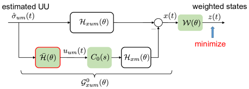
Figure 2: Scheme for unmatched uncertainty attenuation

Existing ${\mathcal{L}_{1}}$AC architectures often rely on the direct inversion of the nominal LTI systems to cancel the effect of unmatched uncertainties (UUs) on the outputs under the assumption that the nominal systems are square and minimum phase [28]. The idea cannot be applied here since it is very challenging, if not impossible, to compute the inverse of an LPV system, or even define it. Here, we propose a new method for unmatched uncertainty attenuation (UUA) based on PPG minimization. The main idea is as follows. With the UU estimation, $\hat{\sigma}_{um}(t)$, we design a feedforward LPV mapping ${\bar{\mathcal{H}}}(\theta)$ to produce a control input $u_{um}(t)$ that tries to minimize the PPG gain from $\hat{\sigma}_{um}(t)$ to the weighted output $z(t)\in\mathbb{R}^{n}$. The idea is shown in Fig. 2, where the weighting function $\mathcal{W}(\theta)$ can be used to tune the frequency range where we want to suppress the effect of the UUs, and emphasize different output channels. $C_{0}(s)$ is a low-pass filter defined by $C_{0}(s)\triangleq\omega_{0}K(s\mathbb{I}_{m}+\omega_{0}K)^{-1},$ which is obtained by plugging a nominal input gain $\omega_{0}$ (selected to be $\mathbb{I}_{m}$ in (43)) into (36). Letting $\mathcal{C}_{0}$ denote the input-output mapping of $C_{0}(s)$, with the architecture in Fig. 2, the mapping from $\hat{\sigma}_{um}(t)$ to $x(t)$ can be represented by $\mathcal{G}_{xum}^{0}(\theta)\triangleq\mathcal{H}_{xum}(\theta)-\mathcal{H}_{xm}(\theta)\mathcal{C}_{0}{\bar{\mathcal{H}}}(\theta)$, which will be exactly $\mathcal{G}_{xum}(\theta)$ in the stability condition (64) if $\omega_{0}=\omega$.

Remark 11.

If we set $\mathcal{W}(\theta)=\textup{diag}(C(\theta),0)$, then $z=[y,0]^{\top\!}$, which means that ${\bar{\mathcal{H}}}(\theta)$ is for attenuating the effect of the UUs on the outputs. This is desired for improving the tracking performance. On the other hand, if we set $\mathcal{W}(\theta)=\mathbb{I}_{n}$, then we have $z=x,$ which indicates that ${\bar{\mathcal{H}}}(\theta)$ is for mitigating the effect of the UUs on all the states. By setting $\mathcal{W}(\theta)=\mathbb{I}_{n}$, we can minimize $\left\lVert\mathcal{G}_{xum}^{0}(\theta)\right\rVert_{\bar{\mathcal{L}}_{1}}$ and potentially $\left\lVert\mathcal{G}_{xum}(\theta)\right\rVert_{\bar{\mathcal{L}}_{1}}$ as well, which allows for the stability condition (64) to hold under more severe uncertainties. Thus, $\mathcal{W}(\theta)$ can be tuned to balance the tracking performance and the robustness margin for satisfying the stability condition (64).

Remark 12.

We design ${\bar{\mathcal{H}}}(\theta)$ to minimize the PPG as the performance index from the UUs to the weighted states, because we aim to provide a transient performance guarantee. If the transient performance is not a major concern, then other performance indices can be utilized, such as $\mathcal{L}_{2}$ gain.

Remark 13.

The proposed approach for UUA can be easily adapted for LTI systems. It does not need strict-feedback forms required in backstepping based approaches [32, 33, 34, 42], and relaxes square system and non-minimum phase assumptions needed in dynamic inversion based approaches [28]. Combined with the small-gain theorem (used to derive (64)), our approach deals with state- and time-dependent uncertainties, unlike the $H_{\infty}$ [31] and coordinate transformation [43] approaches that handle only bounded disturbances.

Next, we will show how to design the mapping ${\bar{\mathcal{H}}}(\theta)$ leveraging the multivariable feedback control theory [40] and its extension to LPV systems [4, 44]. Let us denote the state-space realization of $\mathcal{W}(\theta)$ as $\left(A_{\mathcal{W}}(\theta),B_{\mathcal{W}}(\theta),C_{\mathcal{W}}(\theta),D_{\mathcal{W}}(\theta)\right)$, and the order of $\mathcal{W}(\theta)$, i.e., the number of state variables, as $n_{\mathcal{W}}$. The generalized plant for designing ${\bar{\mathcal{H}}}(\theta)$ is then given by

$$\dot{\bar{x}}(t) =\bar{A}(\theta)\bar{x}(t)+{{\bar{B}}_{1}}(\theta){\hat{\sigma}_{um}}(t)+{{\bar{B}}_{2}}(\theta){u_{um}}(t),$$

$$z(t) ={{\bar{C}}_{1}}(\theta)\bar{x}(t)+{{\bar{D}}_{11}}(\theta){\hat{\sigma}_{um}}(t)+{{\bar{D}}_{12}}(\theta){u_{um}}(t),$$ (47)

$$\bar{y}(t) ={{\bar{C}}_{2}}(\theta)\bar{x}(t)+{{\bar{D}}_{21}}(\theta){\hat{\sigma}_{um}}(t),\vspace{-3mm}$$

where $\bar{x}\triangleq\left[\begin{array}[]{*{20}{c}}{{x_{um}^{\top\!}}}&{{x_{m}^{\top\!}}}&{{x_{\mathcal{W}}^{\top\!}}}\end{array}\right]^{\top\!}$,

$$\left[{\begin{array}[]{*{20}{c}}{\bar{A}}&\vline&{{{\bar{B}}_{1}}}&\vline&{{{\bar{B}}_{2}}}\\ \hline\cr{{{\bar{C}}_{1}}}&\vline&{{{\bar{D}}_{11}}}&\vline&{{{\bar{D}}_{12}}}\\ \hline\cr{{{\bar{C}}_{2}}}&\vline&{{{\bar{D}}_{21}}}&\vline&\end{array}}\right]\triangleq{\left[{\begin{array}[]{*{20}{c}}{{A_{m}}}&0&0&\vline&{{B_{u}}}&\vline&0\\ 0&{{A_{m}}}&0&\vline&0&\vline&{{B}}\\ {{B_{\mathcal{W}}}{C}}&{{B_{\mathcal{W}}}{C}}&{{A_{\mathcal{W}}}}&\vline&0&\vline&0\\ \hline\cr{{D_{\mathcal{W}}}{C}}&{{D_{\mathcal{W}}}{C}}&{{C_{\mathcal{W}}}}&\vline&0&\vline&0\\ \hline\cr 0&0&0&\vline&{{\mathbb{I}_{n-m}}}&\vline&\end{array}}\right]},$$

with the dependence of the matrices on $\theta$ omitted. Here, $x_{um}(t)\in\mathbb{R}^{n}$, $x_{m}(t)\in\mathbb{R}^{n}$ and $x_{W}(t)\in\mathbb{R}^{n_{\mathcal{W}}}$ are the state variables associated with $\mathcal{H}_{um}(\theta)$, $\mathcal{H}_{m}(\theta)$ and $\mathcal{W}(\theta)$, respectively. Obviously, the dimension of the generalized plant in (47) is $\bar{n}=2n+n_{\mathcal{W}}$. We consider ${\bar{\mathcal{H}}}(\theta)$ of the same order as the generalized plant (47) with the state-space realization:

$$\left\{\begin{aligned} \dot{x}_{\bar{\mathcal{H}}}(t)&=A_{\bar{\mathcal{H}}}(\theta)x_{\bar{\mathcal{H}}}(t)+B_{\bar{\mathcal{H}}}(\theta)\bar{y}(t)\\ u_{um}(t)&=C_{\bar{\mathcal{H}}}(\theta)x_{\bar{\mathcal{H}}}(t)+D_{\bar{\mathcal{H}}}(\theta)\bar{y}(t)\end{aligned}\right.,$$ (48)

where $x_{\bar{\mathcal{H}}}(t)\in\mathbb{R}^{\bar{n}}$. The following lemma presents synthesis conditions for designing ${\bar{\mathcal{H}}}(\theta)$ in order to minimize the PPG from $\hat{\sigma}_{um}(t)$ to $z(t)$.

Lemma 8.

Consider the LPV generalized plant in (47) subject to Assumption 1. There exists an LPV controller (48) enforcing internal stability and a bound $\gamma$ on the PPG of the closed-loop system, whenever there exist PD symmetric matrices $X(\theta)$ and $Y(\theta)$, a PD quadruple of state-space data ($\hat{A}(\theta),\hat{B}(\theta),\hat{C}(\theta),\hat{D}(\theta)$) and positive constants $\mu$ and $\upsilon$ such that the conditions (53) and (58) hold. In such case, the controller in (48) is given by

$$\left\{\begin{array}[]{ll}{A_{\bar{\mathcal{H}}}}(\theta)=\hat{A}{(X-Y)^{-1}},&{B_{\bar{\mathcal{H}}}}(\theta)=\hat{B},\\ {C_{\bar{\mathcal{H}}}}(\theta)=\hat{C}{(X-Y)^{-1}},&{D_{\bar{\mathcal{H}}}}(\theta)=\hat{D}.\end{array}\right.$$ (49)

$$\left[{\begin{array}[]{*{20}{c}}M_{11}&\star&\star\\ M_{21}&{-\dot{Y}+\left\langle\bar{A}Y\right\rangle+\mu Y}&\star\\ M_{31}&{{\bar{B}}_{1}^{\top}\!\!+\!\bar{D}_{21}^{\top\!}({{\hat{B}}^{\top}}\!\!+\!\hat{D}{\bar{B}}_{2}^{\top})}&{-\upsilon{\mathbb{I}_{n-m}}}\end{array}}\right] <0,$$ (53)

$$\left[{\begin{array}[]{*{20}{c}}{\mu X}&\star&\star&\star\\ {\mu Y}&{\mu Y}&\star&\star\\ 0&0&{(\gamma-\upsilon){\mathbb{I}_{n-m}}}&\star\\ {{{\bar{C}}_{1}}X\!-\!{{\bar{D}}_{12}}\hat{C}}&{{{\bar{C}}_{1}}Y}&{{{\bar{D}}_{11}}\!+\!{{\bar{D}}_{12}}\hat{D}{{\bar{D}}_{21}}}&{\gamma{\mathbb{I}_{n}}}\end{array}}\right] >0,$$ (58)

where $M_{11}\triangleq{-\dot{X}+\left\langle{\bar{A}X-{{\bar{B}}_{2}}\hat{C}}\right\rangle+\mu X}$, $M_{21}\triangleq-\hat{A}-{{\bar{B}}_{2}}\hat{C}+\bar{A}X-\dot{Y}+{{\bar{A}}^{\top}}+\mu{\mathbb{I}_{\bar{n}}}$, $M_{31}\triangleq{{{({{\bar{B}}_{1}}+{{\bar{B}}_{2}}\hat{D}{{\bar{D}}_{21}})}^{\top}}}$.

Proof. The proof is built upon a preliminary lemma, i.e., Lemma 13, given in Appendix A-B. The equations 49, 53 and 58 can be derived from 140, 141 and 146 in Lemma 13 in two steps. The first step is to do a congruence transformation, which includes (i) multiplying the left-hand side of (141) by $\rm{diag}(\mathbb{I}_{\bar{n}},\tilde{Y}^{-1}(\theta),\mathbb{I}_{n-m})$ and its transpose from the left and right, and (ii) multiplying the left-hand side of (146) by $\rm{diag}(\mathbb{I}_{\bar{n}},\tilde{Y}^{-1}(\theta),\mathbb{I}_{n-m},\mathbb{I}_{n})$ and its transpose from the left and right. The second step is to introduce new variables $X(\theta)$, $Y(\theta)$ such that $X(\theta)=\tilde{X}(\theta)$, $Y(\theta)=\tilde{Y}^{-1}(\theta)$. Since both of these two steps induce equivalent transformations, the result directly follows from Lemma 13 in Appendix A-B. $\blacksquare$

Remark 14.

Similar to the computation of a PPG bound of a given LPV system according to Lemma 5, a line search for $\mu$ is needed. Also, since $\gamma$ appears linearly in the synthesis conditions in Lemma 8, we can design the mapping ${\bar{\mathcal{H}}}(\theta)$ to minimize $\gamma$.

Remark 15.

Lemma 8 presents the LMI conditions for synthesizing dynamic feedforward LPV controllers for PPG minimization, which do not need the derivatives of scheduling parameters for implementation, without imposing restrictive structures on the Lyapunov functions (see [4, Section III] and Remark 24).

For performance analysis in Section V (more specifically in Lemma 11), we define

$$\mathcal{F}(\theta)\triangleq{\mathcal{C}}\left({B^{\dagger}(\theta)+\bar{\mathcal{H}}(\theta)B_{u}^{\dagger}(\theta)}\right),$$ (59)

where $B^{\dagger}(\theta)$ and $B_{u}^{\dagger}(\theta)$ are the pseudo-inverse of $B(\theta)$ and $B_{u}(\theta)$, respectively. Then, under zero initial states, given the signal ${\tilde{\sigma}}(t)\in\mathbb{R}^{n}$ (defined later in (76a)) to $\mathcal{F}(\theta)$ as the input, the output $y_{\mathcal{F}}(t)\in\mathbb{R}^{m}$ can be computed as

$$\begin{split}{{\dot{x}_{\mathcal{F}}}}(t)&={A_{\mathcal{F}}}(\theta){x_{\mathcal{F}}}(t)+{B_{\mathcal{F}}}(\theta){{\tilde{\sigma}}}(t),\quad x_{\mathcal{F}}(0)=0,\\ y_{\mathcal{F}}(t)&={C_{\mathcal{F}}}(\theta){x}_{\mathcal{F}}(t),\end{split}$$ (60)

where $A_{\mathcal{F}}(\theta)$, $B_{\mathcal{F}}(\theta)$ and $C_{\mathcal{F}}(\theta)$ are the state-space matrices. Since both ${\bar{\mathcal{H}}}(\theta)$ and $\mathcal{C}$ are stable, $\mathcal{F}(\theta)$ is also stable. In order to establish the bound on $y_{\mathcal{F}}(t)$ given a bounded ${\tilde{\sigma}}(t)$ to $\mathcal{F}(\theta)$ later in Lemma 11, we make the following assumption.

Assumption 8.

There exists a PD symmetric matrix $P_{\mathcal{F}}(\theta)$ and a constant $\mu_{\mathcal{F}}$ such that

$$\left\langle\!A_{\mathcal{F}}^{\top\!}(\theta)P_{\mathcal{F}}(\theta)\!\right\rangle\!+\!\dot{P}_{\mathcal{F}}(\theta) \!\leq\!-\mu_{\mathcal{F}}P_{\mathcal{F}}(\theta),\ \forall(\theta,\dot{\theta})\in\Theta\!\times\!\Theta_{d},$$

$$P_{\mathcal{F}}(\theta) >0,\ \forall\theta\in\Theta.$$ (61)

Remark 16.

Assumption 8 essentially means that there exists a quadratic PD Lyapunov function $V(t,\theta)\triangleq x_{\mathcal{F}}^{\top\!}(t)P_{\mathcal{F}}(\theta)x_{\mathcal{F}}(t)$ guaranteeing the stability of the system defined in (60).

Remark 17.

The only decision variables in (61) are $P_{\mathcal{F}}(\theta)$ and $\mu_{\mathcal{F}}$. Thus, Assumption 8 can be verified by performing a line search for $\mu_{\mathcal{F}}$ and solving a PD-LMI problem for each $\mu_{\mathcal{F}}$.

IV-C Computational perspectives

Solving PD-LMI conditions: Up to now, LMI technique is still the most common and effective technique for analysis and control synthesis for LPV systems [38, Section 1.3]. Therefore, it is no surprise that (PD-)LMIs are adopted in this work for (i) determining the state bounds for autonomous LPV systems (Lemma 3), (ii) computing the PPG bounds for LPV systems (Lemma 5) and (iii) designing the feedforward mapping for unmatched uncertainty attention (Lemma 8). The PD-LMIs can be solved by applying the gridding technique for general parameter dependence [4]. Under special circumstances like polynomial parameter dependence, techniques such as sum-of-square relaxations [45] can be employed to obtain a finite number of sufficient LMI conditions, which can then be solved efficiently using off-the-shelf packages and solvers.

Incorporation of unknown input gain matrix: In the presence of uncertain input gain, to verify the stability condition in (64), we need to compute the PPG bounds of several mappings (i.e., $\mathcal{G}_{xm}(\theta),\ \mathcal{G}_{xum}(\theta)$ and $\mathcal{H}_{xm}(\theta)\mathcal{C}K_{r}(\theta)$) involving the uncertain input gain $\omega$. Therefore, $\omega$ will appear in the LMI conditions 26 and 27 when we apply Lemma 5. Fortunately, under proper state-space realizations, $\omega$ will appear linearly in the state-space matrices of those mappings (as demonstrated in Appendix B), and thus appear linearly in the LMI conditions in Lemma 5. Considering that $\mathrm{vec}(\omega)\in\hat{\Omega}$ with $\hat{\Omega}$ being a polytope (Assumption 3), to account for the uncertainty in $\omega$, we can formulate robust LMI conditions using the vertices of $\hat{\Omega}$; the resulting LMIs will be independent of $w$.

V Stability and Performance Analysis

In this section, we will analyze the performance of the adaptive closed-loop system with the controller defined in 43, 44 and 46, and derive performance bounds for both transient and steady-state phases under certain conditions. The characterization of the performance of the adaptive system uses a non-adaptive reference system, defined as

$$\dot{x}_{\textup{r}}(t) =A_{m}\left(\theta\right)x_{\textup{r}}(t)+B\left(\theta\right)\left(\omega u_{\textup{r}}(t)+f_{1}(t,x_{\textup{r}}(t)\right)+B_{u}(\theta)f_{2}(t,x_{\textup{r}}(t)),\ x_{\textup{r}}(0)=x_{0},$$

$$u_{\textup{r}} =-\omega^{-1}\mathcal{C}\left(\eta_{1\textup{r}}+{\bar{\mathcal{H}}}(\theta)\eta_{2\textup{r}}-K_{r}(\theta)r\right),$$ (62)

$$y_{\textup{r}}(t) =C(\theta)x_{\textup{r}}(t),$$

where

$$\eta_{i\textup{r}}(t)\triangleq f_{i}(t,x_{\textup{r}}(t)),\quad i=1,2.$$ (63)

It can be seen that the control law in the reference system aims to partially cancel the matched uncertainty within the bandwidth of the filter $\mathcal{C}(s)$ and reject the unmatched uncertainty based on the idea introduced in Section IV-B. Moreover, the control law utilizes the true uncertainties and is thus not implementable. Therefore, the reference system is only used to help characterize the performance of the adaptive system. With the reference system, performance analysis of the adaptive system will be performed in four steps: (i) establish the boundedness of the reference system (Lemma 9); (ii) quantify the difference between the state, input and output signals of the adaptive system and those of the reference system (Theorem 1); (iii) quantify the difference between the state, input and output signals of the reference system and those of the ideal system (Lemma 12); (iv) based on the results from (ii) and (iii), quantify the difference between the state, input and output signals of the adaptive system and those of the ideal system (Theorem 2).

V-A Stability condition

Given the uncertain system dynamics in 12, a constant $\rho_{0}$ (the bound on $\left\lVert x_{0}\right\rVert$), a baseline controller 3 that guarantees the stability of the nominal CL system (Assumption 2), and the prior knowledge of uncertainties represented in Assumptions 3, 5, 6 and 4, for guaranteeing the stability and tracking performance, the design of $K$ in 36 needs to ensure that there exists a positive constant $\rho_{r}$ such that the following condition holds:

$$\left\lVert\mathcal{G}_{xm}(\theta)\right\rVert_{\bar{\mathcal{L}}_{1}}({L_{f_{1}}^{\rho}\rho_{r}+b_{f_{1}}^{0}})+\left\lVert\mathcal{G}_{xum}(\theta)\right\rVert_{\bar{\mathcal{L}}_{1}}({L_{f_{2}}^{\rho}\rho_{r}+b_{f_{2}}^{0}})<{\rho_{r}-\left\lVert\mathcal{H}_{xm}(\theta)\mathcal{C}K_{r}(\theta)\right\rVert_{\bar{\mathcal{L}}_{1}}\left\lVert r\right\rVert_{\mathcal{L}_{\infty}}-\rho_{\textup{in}}},$$ (64)

where $\mathcal{C}$ denotes the input-output mapping of $\mathcal{C}(s)$, and

$$\rho \triangleq\rho_{r}+\gamma_{1},$$ (65)

with ${\gamma}_{1}$ being a positive constant that is selected by users and therefore can be arbitrarily small. Additionally, $L_{f_{i}}^{\rho}$ $(i=1,2)$ are defined in 18g and 18f, $K_{r}(\theta)$ is the feedforward gain introduced in (4), and $\mathcal{G}_{xm}(\theta)$ and $\mathcal{G}_{xum}(\theta)$ are defined in 39.

Remark 18.

The condition in (64) will be used to guarantee the stability of a non-adaptive reference system (defined later in (62)) and derive the performance bounds of the closed-loop adaptive system with respect to the reference system (see Theorem 1) in Section V. More specifically, we will show that the states of the reference system and the adaptive systems are bounded by $\rho_{r}$ and $\rho$, respectively, while the bound on their difference, i.e., $\gamma_{1}$, can be made arbitrarily small.

Also, the stability condition (64) uses PPG bounds instead of ${\mathcal{L}_{1}}$ norms, generally used in existing ${\mathcal{L}_{1}}$AC work with desired dynamics represented by LTI models [17]. This is because for LPV systems it is difficult to compute the ${\mathcal{L}_{1}}$ norm exactly, while an upper bound for the PPG can be computed using LMIs, as shown in Lemma 5.

Remark 19.

In the absence of UUs, condition (64) degrades to $\left\lVert\mathcal{G}_{xm}(\theta)\right\rVert_{\bar{\mathcal{L}}_{1}}({L_{f_{1}}^{\rho}\rho_{r}+b_{f_{1}}^{0}})<\rho_{r}-\left\lVert\mathcal{H}_{xm}(\theta)\mathcal{C}K_{r}(\theta)\right\rVert_{\bar{\mathcal{L}}_{1}}\cdot\\ \left\lVert r\right\rVert_{\mathcal{L}_{\infty}}-\rho_{\textup{in}},$ which can always be satisfied by increasing the filter bandwidth since $\mathcal{G}_{xm}(\theta)$ tends towards $0$ when the filter bandwidth becomes infinite. Additionally, if all the terms in (64) except $\rho_{r}$ are finite and $L_{f_{i}}^{\rho}$ ($i=1,2$) are sufficiently small regardless of $\rho_{r}$ (meaning that the uncertainties $f_{i}(t,x)$ ($i=1,2$) change sufficiently slowly with respect to $x$), such that $\left\lVert\mathcal{G}_{xm}(\theta)\right\rVert_{\bar{\mathcal{L}}_{1}}L_{f_{1}}^{\rho}+\left\lVert\mathcal{G}_{xum}(\theta)\right\rVert_{\bar{\mathcal{L}}_{1}}L_{f_{2}}^{\rho}<1$, then we can always find a large enough $\rho_{r}$ such that (64) holds.

Remark 20.

The condition in (64) could be rather conservative because it is derived using small gain theorem (see the proof of Lemma 9), and furthermore, the PPG bound computed using LMI techniques could be quite loose. Nevertheless, it provides a verifiable way for theoretic guarantees, when addressing the challenging problem of adaptive control of LPV systems subject to unmatched nonlinear uncertainties.

V-B Boundedness of the reference system

We now present a lemma to establish the boundedness of the reference system.

Lemma 9.

Given the closed-loop reference system in (62), if Assumption 2, conditions 17 and 15, and the stability condition (64) hold, we have

$$\left\lVert x_{\textup{r}}\right\rVert_{\mathcal{L}_{\infty}} <\rho_{r},\quad\left\lVert u_{\textup{r}}\right\rVert_{\mathcal{L}_{\infty}}<\rho_{ur},$$ (66)

where

$$\rho_{ur}\triangleq \left\lVert\omega^{-1}\mathcal{C}(s)\right\rVert_{\mathcal{L}_{1}}\left(\max_{\theta\in\Theta}\left\lVert K_{r}(\theta)\right\rVert\left\lVert r\right\rVert_{\mathcal{L}_{\infty}}+L_{f_{1}}^{\rho_{r}}{\rho_{r}}+b_{f_{1}}^{0}+\left\lVert{\bar{\mathcal{H}}}(\theta)\right\rVert_{\bar{\mathcal{L}}_{1}}(L_{f_{2}}^{\rho_{r}}{\rho_{r}}+b_{f_{2}}^{0})\right).$$ (67)

Proof. It follows from (62), the definition of $\mathcal{H}_{xm}(\theta)$ above (37), and the definitions of $\mathcal{G}_{xm}(\theta)$ and $\mathcal{G}_{xum}(\theta)$ in (39) that

$$x_{\textup{r}}=\mathcal{G}_{xm}(\theta)\eta_{1\textup{r}}+\mathcal{G}_{xum}(\theta)\eta_{2\textup{r}}+\mathcal{H}_{xm}(\theta)\mathcal{C}K_{r}(\theta)r+x_{\textup{in}}.$$

Due to Assumption 2, according to Lemma 4, we have

$$\left\lVert x_{\textup{r}}\right\rVert_{\mathcal{L}_{\infty}^{[0,\tau]}}\leq\left\lVert x_{\textup{in}}\right\rVert_{\mathcal{L}_{\infty}}+\left\lVert\mathcal{G}_{xm}(\theta)\right\rVert_{\bar{\mathcal{L}}_{1}}\left\lVert\eta_{1\textup{r}}\right\rVert_{\mathcal{L}_{\infty}^{[0,\tau]}}+\left\lVert\mathcal{G}_{xum}(\theta)\right\rVert_{\bar{\mathcal{L}}_{1}}\!\left\lVert\eta_{2\textup{r}}\right\rVert_{\mathcal{L}_{\infty}^{[0,\tau]}}+\left\lVert\mathcal{H}_{xm}(\theta)\mathcal{C}K_{r}(\theta)\right\rVert_{\bar{\mathcal{L}}_{1}}\!\left\lVert r\right\rVert_{\mathcal{L}_{\infty}}\!.$$ (68)

If the bound on $x_{\textup{r}}$ in (66) is not true, since $\left\lVert x_{\textup{r}}(0)\right\rVert=\left\lVert x_{0}\right\rVert<\rho_{r}$ and $x_{\textup{r}}(t)$ is continuous, then there exists $\tau>0$ such that $\left\lVert x_{\textup{r}}(t)\right\rVert<\rho_{r}$, for any $t\in[0,\tau)$, and $\left\lVert x_{\textup{r}}(\tau)\right\rVert=\rho_{r},$ which implies that

$$\left\lVert x_{\textup{r}}\right\rVert_{\mathcal{L}_{\infty}^{[0,\tau]}}=\rho_{r}.$$ (69)

Further considering conditions 17 and 15, we have

$$\left\lVert\eta_{i\textup{r}}\right\rVert_{\mathcal{L}_{\infty}^{[0,\tau]}}\leq L_{f_{i}}^{\rho_{r}}\rho_{r}+b_{f_{i}}^{0},\quad i=1,2.$$ (70)

Plugging the preceding inequality into (68) results in $\left\lVert x_{\textup{r}}\right\rVert_{\mathcal{L}_{\infty}^{[0,\tau]}}\leq\left\lVert x_{\textup{in}}\right\rVert_{\mathcal{L}_{\infty}}+\left\lVert\mathcal{G}_{xm}(\theta)\right\rVert_{\bar{\mathcal{L}}_{1}}(L_{f_{1}}^{\rho_{r}}\rho_{r}+b_{f_{1}}^{0})+\left\lVert\mathcal{G}_{xum}(\theta)\right\rVert_{\bar{\mathcal{L}}_{1}}\cdot\\ (L_{f_{2}}^{\rho_{r}}\rho_{r}+b_{f_{2}}^{0})+\left\lVert\mathcal{H}_{xm}(\theta)\mathcal{C}K_{r}(\theta)\right\rVert_{\bar{\mathcal{L}}_{1}}\left\lVert r\right\rVert_{\mathcal{L}_{\infty}}<\rho_{r}-\rho_{\textup{in}}+\left\lVert x_{\textup{in}}\right\rVert_{\mathcal{L}_{\infty}}\leq\rho_{r},$ where the third and last inequalities are due to (64) (together with the fact that $L_{f_{i}}^{\rho_{r}}\leq L_{f_{i}}^{\rho}$ for $i=1,2$) and (21), respectively. As a result, we arrive at $\left\lVert x_{\textup{r}}\right\rVert_{\mathcal{L}_{\infty}^{[0,\tau]}}<\rho_{r}$, contradicting (69). This proves the bound on $x_{\textup{r}}$ in (66). Using 66 and 70 and the definition of $u_{\textup{r}}$ in (62), we obtain the bound on $u_{\textup{r}}$ in (66). $\blacksquare$

Let $\bar{\gamma}_{0}$ be a small positive constant such that

$$\frac{\left\lVert\mathcal{H}_{xm}(\theta)\right\rVert_{\bar{\mathcal{L}}_{1}}}{1-\left\lVert\mathcal{G}_{xm}(\theta)\right\rVert_{\bar{\mathcal{L}}_{1}}L_{f_{1}}^{\rho}-\left\lVert\mathcal{G}_{xum}(\theta)\right\rVert_{\bar{\mathcal{L}}_{1}}L_{f_{2}}^{\rho}}\bar{\gamma}_{0}<\gamma_{1},$$ (71)

where $\gamma_{1}$ is introduced in 65. We further define

$$\rho_{u}\triangleq\rho_{ur}+\gamma_{2},$$ (72)

$$\gamma_{2}\triangleq\left({{{\|{{\omega^{-1}}{\mathcal{C}}}\|}_{{{\mathcal{L}}_{1}}}}{L_{f_{1}}^{\rho}}\!+\!{{\|{{\omega^{-1}}{\mathcal{C}}\bar{\mathcal{H}}(\theta)}\|}_{{{\bar{\mathcal{L}}}_{1}}}}{L_{f_{2}}^{\rho}}}\right){\gamma_{1}}\!+\!\|{{\omega^{-1}}}\|{{\bar{\gamma}}_{0}}.$$ (73)

We will show (in Theorem 1) that $\rho$ and $\rho_{u}$ in (65) and (72) are the bounds for the states and inputs of the adaptive closed-loop system with the controller defined by 43, 44 and 46.

V-C Transient and steady-state performance

For the derivations in this section, let us first define

$$\eta_{i}(t) \triangleq f_{i}(t,x(t)),\quad i=1,2,$$ (74a)

$$\tilde{\eta}_{m}(t) \triangleq\hat{\sigma}_{m}(t)-\left((\omega-\mathbb{I}_{m})u(t)+\eta_{1}(t)\right),\quad$$ (74b)

$$\tilde{\eta}_{um}(t) \triangleq\hat{\sigma}_{um}(t)-\eta_{2}(t).$$ (74c)

From 12aand 43, we obtain the prediction error dynamics:

$$\dot{\tilde{x}}(t)=-a\tilde{x}(t)+\hat{\sigma}(t)-B(\theta)(\omega-\mathbb{I}_{m})u(t)-{{\bar{f}}(t,x(t))}=-a\tilde{x}(t)+\hat{\sigma}(t)-\sigma(t,x(t),u(t)),\ \tilde{x}(0)=0,$$ (75)

where $\sigma(t,x(t),u(t))$ is defined in 42. Recalling from (45) that $\hat{\sigma}(t)=B(\theta)\hat{\sigma}_{m}(t)+B_{u}(\theta)\hat{\sigma}_{um}(t),$ and considering (11), (42) and (74), we have

$${\tilde{\sigma}}(t) \triangleq\hat{\sigma}(t)-\sigma(t,x(t),u(t))$$ (76a)

$$=B(\theta)\tilde{\eta}_{m}(t)+B_{u}(\theta)\tilde{\eta}_{um}(t),$$ (76b)

which further implies that

$$\begin{bmatrix}\tilde{\eta}_{m}(t)\\ \tilde{\eta}_{um}(t)\end{bmatrix}=\begin{bmatrix}B^{\dagger}(\theta)\\ B_{u}^{\dagger}(\theta)\end{bmatrix}\tilde{\sigma}(t).$$ (77)

For following derivations, let us first define

$$b_{\sigma}(\rho,\rho_{u})\triangleq \ b_{B}\max_{\omega\in\Omega}\left\lVert\omega\!-\!\mathbb{I}_{m}\right\rVert(\rho_{u}{+b_{K_{x}}\rho})+L_{f}^{\rho}\rho+b_{f}^{0},$$ (78)

$$b_{\dot{x}}(\rho,\rho_{u})\triangleq \ b_{A_{m}}\rho+b_{B}\rho_{u}\max_{\omega\in\Omega}\left\lVert\omega\right\rVert+L_{f}^{\rho}\rho+b_{f}^{0}{+b_{B}\max\limits_{\omega\in\Omega}\left\lVert(\omega\!-\!\mathbb{I}_{m})\right\rVert b_{K_{x}}\rho},$$ (79)

$$b_{\hat{\sigma}}(\rho,\rho_{u})\triangleq \ e^{-aT}\sqrt{n}~{}b_{\sigma}(\rho,\rho_{u}),$$ (80)

$$b_{\dot{u}}(\rho,\rho_{u})\triangleq \ \left\|K\right\|\left[{{\rho_{u}}}+(1+\left\|{\bar{\mathcal{H}}(\theta)}\right\|_{{\bar{\mathcal{L}}}_{1}})b_{B^{\dagger}}{b_{\hat{\sigma}}}(\rho,{\rho_{u}})+b_{K_{r}}{\left\|r\right\|}_{{\mathcal{L}}_{\infty}}\right],$$ (81)

$$b_{{\tilde{\sigma}}}(\rho,\rho_{u})\triangleq \ 2\sqrt{n}~{}T\left[\left\|{\omega-{\mathbb{I}_{m}}}\right\|({{b_{{B}}}{b_{\dot{u}}}(\rho,{\rho_{u}})+L_{B}{b_{\dot{\theta}}}{\rho_{u}}})+{l_{f}}+{L_{f}^{\rho}}{b_{\dot{x}}}(\rho,{\rho_{u}})\right]+(1-e^{-aT})\sqrt{n}~{}b_{\sigma}(\rho,\rho_{u}).\vspace{-8mm}$$ (82)

Lemma 10.

Given the uncertain system in (12) satisfying Assumptions 7, 6, 5, 4 and 3, the state predictor in (43) and the adaptive law in (44), if

$$\left\lVert x\right\rVert_{\mathcal{L}_{\infty}^{[0,\tau]}}\leq\rho,\quad\left\lVert u\right\rVert_{\mathcal{L}_{\infty}^{[0,\tau]}}\leq\rho_{u},$$ (83)

then

$$\left\lVert{\tilde{\sigma}}(t)\right\rVert \leq\left\{\begin{array}[]{l}b_{\sigma}(\rho,\rho_{u}),\quad\forall t\in[0,T),\\ b_{{\tilde{\sigma}}}(\rho,\rho_{u}),\quad\forall t\in[T,\tau].\end{array}\right.$$ (86)

Proof. In the following proof, we often omit the dependence of $\sigma$ on $x$ and $u$, i.e., simply writing $\sigma(t)$ for $\sigma(t,x(t),u(t))$, for notation brevity. As explained in the proof of Lemma 1, Assumptions 5 and 4 imply $\left\lVert f(t,x)\right\rVert\leq L_{f}^{\rho}\rho+b_{f}^{0}$, for all $\left\lVert x\right\rVert\leq\rho$ and for all $t\geq 0$, which, together with the definition of ${\bar{f}}(t,x)$ in 11 and (83), indicate

$$\left\lVert{\bar{f}}(t,x)\right\rVert\leq L_{f}^{\rho}\rho+b_{f}^{0}+b_{B}\max\limits_{\omega\in\Omega}\left\lVert(\omega\!-\!\mathbb{I}_{m})\right\rVert b_{K_{x}}\rho,\quad\forall t\in[0,\tau].$$ (87)

From 87 and the definition of $\sigma(t,x,u)$ in (42), we have

$$\left\lVert\sigma(t,x,u)\right\rVert\leq\left\lVert B(\theta)\right\rVert\left\lVert\omega-\mathbb{I}_{m}\right\rVert\rho_{u}+\left\lVert{{\bar{f}}(t,x)}\right\rVert\leq L_{f}^{\rho}\rho+b_{f}^{0}+b_{B}\max_{\omega\in\Omega}\left\lVert\omega\!-\!\mathbb{I}_{m}\right\rVert(\rho_{u}\!+\!b_{K_{x}}\rho)=b_{\sigma}(\rho,\rho_{u}),$$ (88)

for any $t$ in $[0,\tau]$. Equations 87, 12a and 83 imply

$$\left\lVert\dot{x}(t)\right\rVert\leq\left\lVert A_{m}(\theta)\right\rVert\left\lVert x(t)\right\rVert+\left\lVert B(\theta)\right\rVert\left\lVert\omega\right\rVert\left\lVert u(t)\right\rVert+\left\lVert{{\bar{f}}(t,x)}\right\rVert\leq b_{\dot{x}}(\rho,\rho_{u}),\quad\forall t\in[0,\tau],$$ (89)

where $b_{\dot{x}}(\rho,\rho_{u})$ is defined in (79). From the prediction error dynamics in (75), we have for $0\leq t<T$, $i\in\mathbb{Z}_{0}$,

$$\tilde{x}(iT+t)=e^{-at}\tilde{x}(iT)\!+\!\int_{iT}^{iT+t}\!e^{-a(iT+t-\xi)}(\hat{\sigma}(\xi)\!-\!\sigma(\xi))d\xi=e^{-at}\tilde{x}(iT)+\int_{iT}^{iT+t}\!e^{-a(iT+t-\xi)}(\hat{\sigma}(iT)\!-\!\sigma(\xi))d\xi,\vspace{-3mm}$$ (90)

which implies that for $i\in\mathbb{Z}_{0}$, $\tilde{x}((i\!+\!1)T)=e^{-aT}\tilde{x}(iT)\!+\!\int_{iT}^{(i\!+\!1)T}e^{-a((i\!+\!1)T-\xi)}\hat{\sigma}(iT)d\xi-\int_{iT}^{(i\!+\!1)T}e^{-a((i\!+\!1)T-\xi)}\sigma(\xi)d\xi$. Plugging the adaptive law in (44) into the above equation gives

$$\tilde{x}((i+1)T)=-\int_{iT}^{(i+1)T}e^{-a((i+1)T-\xi)}\sigma(\xi)d\xi.$$ (91)

Furthermore, since $e^{-a((i+1)T-\xi)}$ is always positive and $\sigma(\xi)$ is continuous, we can apply the first mean value theorem in an element-wise manner to (91). Doing this gives $\tilde{x}((i+1)T)=-\int_{iT}^{(i+1)T}e^{-a((i+1)T-\xi)}d\xi\bm{[}\sigma_{j}(\tau_{j}^{*})\bm{]}$, further implying

$$\tilde{x}((i+1)T)=-\frac{1}{a}(1-e^{-aT})\bm{[}\sigma_{j}(\tau_{j}^{*})\bm{]},$$ (92)

for some $\tau_{j}^{*}\in(iT,(i+1)T)$, for $j\in\mathbb{Z}_{1}^{n}$ and $i\in\mathbb{Z}_{0}$, where $\sigma_{j}(t)$ is the $j$-th element of $\sigma(t)$, and

$$\bm{[}\sigma_{j}(\tau_{j}^{*})\bm{]}\triangleq[\sigma_{1}(\tau_{1}^{*}),\sigma_{2}(\tau_{2}^{*}),\cdots,\sigma_{n}(\tau_{n}^{*})]^{\top\!}.$$

The adaptive law in (44) and the equality (92) indicate that for any $t\in\left[(i+1)T,(i+2)T\right)\\ \cap[0,\tau]$ with $i\in\mathbb{Z}_{0}$, there exist $\tau_{j}^{*}\in(iT,(i+1)T)$ ($j\in\mathbb{Z}_{1}^{n}$) such that

$$\hat{\sigma}(t)=-\frac{a}{e^{aT}-1}\tilde{x}((i+1)T)=e^{-aT}\bm{[}\sigma_{j}(\tau_{j}^{*})\bm{]}.$$ (93)

Note that

$$\left\lVert\sigma(t)-\bm{[}\sigma_{j}(\tau_{j}^{*})\bm{]}\right\rVert\leq\sqrt{n}\left\lVert\sigma(t)-\bm{[}\sigma_{j}(\tau_{j}^{*})\bm{]}\right\rVert_{\infty}=\sqrt{n}\left\lvert\sigma_{j^{\star}_{t}}(t)-{\sigma_{j^{\star}_{t}}(\tau_{j^{\star}_{t}}^{*})}\right\rvert\leq\sqrt{n}\left\lVert\sigma(t)-{\sigma(\tau_{j^{\star}_{t}}^{*})}\right\rVert,$$ (94)

where $j^{\star}_{t}=\arg\max_{j\in\mathbb{Z}_{1}^{n}}\left\lvert\sigma_{j}(t)-{\sigma_{j}(\tau_{j}^{*})}\right\rvert$. Similarly, we have

$$\left\lVert\bm{[}\sigma_{j}(\tau_{j}^{*})\bm{]}\right\rVert \leq\sqrt{n}\left\lvert{\sigma_{{\bar{j}^{\star}}}(\tau_{{\bar{j}^{\star}}}^{*})}\right\rvert\leq\sqrt{n}\left\lVert{\sigma(\tau_{{\bar{j}^{\star}}}^{*})}\right\rVert,$$ (95)

where ${\bar{j}^{\star}}=\arg\max_{j\in\mathbb{Z}_{1}^{n}}\left\lvert{\sigma_{j}(\tau_{j}^{*})}\right\rvert$. The preceding inequality, together with (93), implies that for any $t$ in $[T,\tau]$, we have $\left\lVert\hat{\sigma}(t)\right\rVert\leq e^{-aT}\sqrt{n}~{}b_{\sigma}(\rho,\rho_{u})=b_{\hat{\sigma}}(\rho,\rho_{u}),$ where $b_{\hat{\sigma}}(\rho,\rho_{u})$ is defined in (80). Further considering that $\hat{\sigma}(t)=0$ in $[0,T)$, we have $\left\lVert\hat{\sigma}\right\rVert_{\mathcal{L}_{\infty}^{[0,\tau]}}\leq b_{\hat{\sigma}}(\rho,\rho_{u}).$ On the other hand, the equality in (45) indicates that

$$\left\lVert\begin{bmatrix}[1]{{{\hat{\sigma}}_{m}}}\\ {{{\hat{\sigma}}_{um}}}\end{bmatrix}\right\rVert_{\mathcal{L}_{\infty}^{[0,\tau]}}\leq{\max_{\theta\in\Theta}}\left\|{{\bar{B}^{-1}}(\theta)}\right\|{\left\lVert\hat{\sigma}\right\rVert_{\mathcal{L}_{\infty}^{[0,\tau]}}}\leq{b_{B^{\dagger}}}{b_{\hat{\sigma}}}(\rho,{\rho_{u}}),$$

which, together with the control law in (46), implies

$$\left\lVert\dot{u}\right\rVert_{\mathcal{L}_{\infty}^{[0,\tau]}} \leq\left\|K\right\|\left[{\rho_{u}}+\left\lVert\hat{\sigma}_{m}\right\rVert_{\mathcal{L}_{\infty}^{[0,\tau]}}+{{\left\|{\bar{\mathcal{H}}(\theta)}\right\|}_{{{\bar{\mathcal{L}}}_{1}}}}{\left\lVert\hat{\sigma}_{um}\right\rVert_{\mathcal{L}_{\infty}^{[0,\tau]}}}\!+\!b_{K_{r}}\left\lVert r\right\rVert_{\mathcal{L}_{\infty}}\right]$$

$$\leq\left\|K\right\|\left[{{\rho_{u}}}+\left(1+\left\|{\bar{\mathcal{H}}(\theta)}\right\|_{{\bar{\mathcal{L}}}_{1}}\right)b_{B^{\dagger}}{b_{\hat{\sigma}}}(\rho,{\rho_{u}})\right]+\!\left\|K\right\|b_{K_{r}}{\left\|r\right\|}_{{\mathcal{L}}_{\infty}}\!\!=b_{\dot{u}}(\rho,\rho_{u}).$$ (96)

Define $\tilde{\omega}\triangleq\omega-\mathbb{I}_{m}$. With the bounds on $\left\lVert\dot{x}(t)\right\rVert$ and $\left\lVert\dot{u}(t)\right\rVert$ in (89) and (96), a bound on $\left\|{\sigma(t)-\sigma(\tau_{j^{\star}_{t}}^{*})}\right\|$ (used in (94)) is given by

$$\left\|{\sigma(t)-\sigma(\tau_{j^{\star}_{t}}^{*})}\right\|=\left\|{{B}(\theta(t))\tilde{\omega}u(t)+{\bar{f}}(t,x(t))-{B}(\theta(\tau_{j^{\star}_{t}}^{*}))\tilde{\omega}u(\tau_{j^{\star}_{t}}^{*})-{\bar{f}}(\tau_{j^{\star}_{t}}^{*},x(\tau_{j^{\star}_{t}}^{*}))}\right\|$$

$$=\left\|{{{B}(\theta(t))\tilde{\omega}\left({u(t)-u(\tau_{j^{\star}_{t}}^{*})}\right)+\left({{B}(\theta(t))-{B}(\theta(\tau_{j^{\star}_{t}}^{*}))}\right)\tilde{\omega}u(\tau_{j^{\star}_{t}}^{*})}+{\bar{f}}(t,x(t))-{\bar{f}}(\tau_{j^{\star}_{t}}^{*},x(\tau_{j^{\star}_{t}}^{*}))}\right\|$$

$$\leq\left\|{\tilde{\omega}}\right\|\left({\left\|{{B}(\theta(t))}\right\|\left\|{u(t)-u(\tau_{j^{\star}_{t}}^{*})}\right\|+\left\|{{B}(\theta(t))-{B}(\theta(\tau_{j^{\star}_{t}}^{*}))}\right\|\left\|{u(\tau_{j^{\star}_{t}}^{*})}\right\|}\right)+\left\|{{\bar{f}}(t,x(t))-{\bar{f}}(\tau_{j^{\star}_{t}}^{*},x(\tau_{j^{\star}_{t}}^{*}))}\right\|$$

$$\leq\left\|{\tilde{\omega}}\right\|\left({\left\|{{B}(\theta(t))}\right\|\left\|{\mathop{\smallint}\nolimits_{\tau_{j^{\star}_{t}}^{*}}^{t}\dot{u}(\xi)d\xi}\right\|+\left\|{{B}(\theta(t))-{B}(\theta(\tau_{j^{\star}_{t}}^{*}))}\right\|\left\|{u(\tau_{j^{\star}_{t}}^{*})}\right\|}\right)+{l_{f}}(t-\tau_{j^{\star}_{t}}^{*})+L_{f}^{\rho}\left\|{x(t)-x(\tau_{j^{\star}_{t}}^{*})}\right\|$$

$$\leq\left\|{\tilde{\omega}}\right\|\left({{b_{{B}}}\mathop{\smallint}\nolimits_{\tau_{j^{\star}_{t}}^{*}}^{t}\left\|{\dot{u}(\xi)}\right\|d\xi+L_{B}\left\|{\theta(t)-\theta(\tau_{j^{\star}_{t}}^{*})}\right\|\left\|{u(\tau_{j^{\star}_{t}}^{*})}\right\|}\right)+{l_{f}}(t-\tau_{j^{\star}_{t}}^{*})+L_{f}^{\rho}\left\|{\mathop{\smallint}\nolimits_{\tau_{j^{\star}_{t}}^{*}}^{t}\dot{x}(\xi)d\xi}\right\|$$ (97a)

$$\leq\left\|{\tilde{\omega}}\right\|\left({{b_{{B}}}{b_{\dot{u}}}(\rho,{\rho_{u}})(t-\tau_{j^{\star}_{t}}^{*})+L_{B}\left\|{\mathop{\smallint}\nolimits_{\tau_{j^{\star}_{t}}^{*}}^{t}\dot{\theta}(\xi)d\xi}\right\|{\rho_{u}}}\right)+{l_{f}}(t-\tau_{j^{\star}_{t}}^{*})+L_{f}^{\rho}{b_{\dot{x}}}(\rho,{\rho_{u}})(t-\tau_{j^{\star}_{t}}^{*})$$ (97b)

$$\leq\!\left({\left\|{\tilde{\omega}}\right\|\!\left({{b_{{B}}}{b_{\dot{u}}}(\rho,{\rho_{u}})\!+\!L_{B}{b_{\dot{\theta}}}{\rho_{u}}}\!\right)\!+\!{l_{f}}\!+\!L_{f}^{\rho}{b_{\dot{x}}}(\rho,{\rho_{u}})}\!\right)(t\!-\!\tau_{j^{\star}_{t}}^{*})\leq 2T\!\left({\left\|{\tilde{\omega}}\right\|\!\left({{b_{{B}}}{b_{\dot{u}}}(\rho,{\rho_{u}})\!+\!L_{B}{b_{\dot{\theta}}}{\rho_{u}}}\!\right)\!+\!{l_{f}}\!+\!{L_{f}^{\rho}}{b_{\dot{x}}}(\rho,{\rho_{u}})}\!\right)$$ (97c)

where 97a is due to 7, 97b is due to 96, and (97c) is due to the fact of $t\in\left[(i+1)T,(i+2)T\right)\cap[0,\tau]$ with $i\in\mathbb{Z}_{0}$ and $\tau_{j^{\star}_{t}}^{*}\in(iT,(i+1)T)$. Therefore, for any $t\in[T,\tau]$, we have $\left\lVert{\tilde{\sigma}}(t)\right\rVert\!=\!\left\lVert\sigma(t)-\hat{\sigma}(t)\right\rVert\!=\!\left\lVert\sigma(t)-e^{-aT}\bm{[}\sigma_{j}(\tau_{j}^{*})\bm{]}\right\rVert\!\leq\!\left\lVert\sigma(t)-\bm{[}\sigma_{j}(\tau_{j}^{*})\bm{]}\right\rVert+(1\!-\!e^{-aT})\left\lVert\bm{[}\sigma_{j}(\tau_{j}^{*})\bm{]}\right\rVert\!\leq\!\sqrt{n}\left\lVert\sigma(t)-{\sigma(\tau_{j^{\star}_{t}}^{*})}\right\rVert\!+\!(1\!-\!e^{-aT})\sqrt{n}\left\lVert{\sigma(\tau_{{\bar{j}^{\star}}}^{*})}\right\rVert,$ where the third equality is due to 93, and the last inequality is due to (94) and 95. Plugging the bounds (88) and (97c) into the preceding inequality and considering the definition in (82) lead to $\left\lVert{\tilde{\sigma}}(t)\right\rVert\leq b_{{\tilde{\sigma}}}(\rho,\rho_{u})$ for any $t\in[T,\tau]$. On the other hand, the inequality (88) and the fact of $\hat{\sigma}(0)=0$ imply $\left\lVert{\tilde{\sigma}}(t)\right\rVert=\left\lVert\sigma(t\right\rVert\leq b_{\sigma}(\rho,\rho_{u})$ for any $t\in[0,T)$. As a result, we have proved (86). $\blacksquare$

Remark 21.

Given finite $\rho$ and $\rho_{u}$ and bounded reference signal $r$ in $[0,\tau]$, the definition in (82) implies $\lim_{T\rightarrow 0}b_{{\tilde{\sigma}}}(\rho,\rho_{u})=0.$ This means that the uncertainty estimation error in $[T,\tau]$ can be made arbitrarily small by decreasing $T$, even in the presence of initialization error, i.e., $\tilde{x}(0)\neq 0$.

Lemma 11.

Given the dynamic mapping $\mathcal{F}(\theta)$ in (60), if Assumption 8 holds and the input ${\tilde{\sigma}}$ is bounded by (86), we have

$$\left\lVert y_{\mathcal{F}}\right\rVert_{\mathcal{L}_{\infty}^{[0,\tau]}}\leq\gamma_{0}(T,\rho,\rho_{u}),$$ (98)

where

$$\gamma_{0}(T,\rho,\rho_{u})\triangleq \max_{\theta\in\Theta}\left\lVert C_{\mathcal{F}}(\theta)\right\rVert\left(\tilde{\lambda}\beta_{\Theta}(T,\mu_{\mathcal{F}},P_{\mathcal{F}},B_{\mathcal{F}})b_{\sigma}(\rho,\rho_{u})+\beta_{\Theta}(\infty,\mu_{\mathcal{F}},P_{\mathcal{F}},B_{\mathcal{F}})b_{{\tilde{\sigma}}}(\rho,\rho_{u})\right),\vspace{-3mm}$$ (99)

with $\tilde{\lambda}\triangleq\sqrt{\frac{{\max_{\theta\in\Theta}{\bar{\lambda}(P_{\mathcal{F}}(\theta))}}}{{\min_{\theta\in\Theta}{\underline{\lambda}(P_{\mathcal{F}}(\theta))}}}}$ and $\beta_{\Theta}(\cdot,\cdot,\cdot,\cdot)$ defined in (30). Furthermore,

$$\lim_{T\rightarrow 0}\gamma_{0}(T,\rho,\rho_{u})=0.$$ (100)

Proof. Since Assumption 8 holds, applying Lemma 7 while considering the bound on ${\tilde{\sigma}}$ in (86) immediately lead to

$$\left\lVert x_{\mathcal{F}}(t)\right\rVert\leq\left\{\!\!\!\begin{array}[]{l}\beta_{\Theta}(T,\mu_{\mathcal{F}},P_{\mathcal{F}},B_{\mathcal{F}})b_{\sigma}(\rho,\rho_{u}),\ \ \forall t\in[0,T],\\ \sqrt{\frac{{\max_{\theta\in\Theta}{\bar{\lambda}(P_{\mathcal{F}}(\theta))}}}{{\min_{\theta\in\Theta}{\underline{\lambda}(P_{\mathcal{F}}(\theta))}}}}\beta_{\Theta}(T,\mu_{\mathcal{F}},P_{\mathcal{F}},B_{\mathcal{F}})b_{\sigma}(\rho,\rho_{u})+\beta_{\Theta}(\infty,\mu_{\mathcal{F}},P_{\mathcal{F}},B_{\mathcal{F}})b_{{\tilde{\sigma}}}(\rho,\rho_{u}),\ \ \forall t\in(T,\tau],\end{array}\right.$$

which further implies $\left\lVert x_{\mathcal{F}}\right\rVert_{\mathcal{L}_{\infty}^{[0,\tau]}}\leq\sqrt{\frac{{\max_{\theta\in\Theta}{\bar{\lambda}(P_{\mathcal{F}}(\theta))}}}{{\min_{\theta\in\Theta}{\underline{\lambda}(P_{\mathcal{F}}(\theta))}}}}\beta_{\Theta}(T,\mu_{\mathcal{F}},P_{\mathcal{F}},B_{\mathcal{F}})b_{\sigma}(\rho,\rho_{u})+\beta_{\Theta}(\infty,\mu_{\mathcal{F}},P_{\mathcal{F}},B_{\mathcal{F}})b_{{\tilde{\sigma}}}(\rho,\rho_{u}).$ The above inequality together with the output equation in (60) immediately gives (98). On the other hand, the definitions in (30) and (82) indicate $\lim_{T\rightarrow 0}\beta_{\Theta}(T,\mu_{\mathcal{F}},P_{\mathcal{F}},B_{\mathcal{F}})=0$ and $\lim_{T\rightarrow 0}b_{{\tilde{\sigma}}}(\rho,\rho_{u})=0$, which, together with the fact that all other terms on the right-hand side of (99) are finite, implies (100). $\blacksquare$

Next, we show that if $T$ is chosen to satisfy

$$\gamma_{0}(T,\rho,\rho_{u})<\bar{\gamma}_{0},$$ (101)

then we can prove the stability and derive the performance bounds of the actual closed-loop adaptive system with respect to the reference system defined in 62.

Theorem 1.

Consider the uncertain system (1) subject to Assumption 1, the control law 6 consisting of the baseline controller 3 and the robust adaptive controller defined via 43, 44 and 46, and the reference system (62). Suppose Assumptions 8, 7, 3, 4, 5, 6 and 2, the stability condition (64) holds with a user-selected constant $\gamma_{1}$ that can be arbitrarily small, and the constraints 71 and 101 hold. Then, we have

$$\left\lVert x\right\rVert_{\mathcal{L}_{\infty}} \leq\rho,$$ (102)

$$\left\lVert u\right\rVert_{\mathcal{L}_{\infty}} \leq\rho_{u},$$ (103)

$$\left\lVert x_{\textup{r}}-x\right\rVert_{\mathcal{L}_{\infty}} \leq\gamma_{1},$$ (104)

$$\left\lVert u_{\textup{r}}-u\right\rVert_{\mathcal{L}_{\infty}} \leq\gamma_{2}.$$ (105)

$$\left\lVert y_{\textup{r}}-y\right\rVert_{\mathcal{L}_{\infty}} \leq b_{C}\gamma_{1},\vspace{-3mm}$$ (106)

where $\rho$, $\rho_{u}$ and $\gamma_{2}$ are defined in 65, 72 and 73, respectively.

Proof. As shown in Section II, under the baseline controller 3, the compositional control law 6 and Assumption 7, we have that (i) the dynamics in (1) is equivalent to (12), and (ii) conditions 17 and 15 hold according to Lemma 1 since Assumptions 3, 1, 7, 4, 5 and 6 hold. We next use contradiction for the proof. Assume that at least one of the bounds in (104) and (105) does not hold. Then, since $\left\lVert x_{\textup{r}}(0)-x(0)\right\rVert=0<\gamma_{1}$, $\left\lVert u_{\textup{r}}(0)-u(0)\right\rVert=0<\gamma_{2}$, and $x(t)$, $x_{\textup{r}}(t)$, $u(t)$ and $u_{\textup{r}}(t)$ are continuous, there exists $\tau>0$ such that $\left\lVert x_{\textup{r}}(\tau)-x(\tau)\right\rVert=\gamma_{1}\ \textup{or}\ \left\lVert u_{\textup{r}}(\tau)-u(\tau)\right\rVert=\gamma_{2},$ while $\left\lVert x_{\textup{r}}(t)-x(t)\right\rVert<\gamma_{1}$ and $\left\lVert u_{\textup{r}}(t)-u(t)\right\rVert<\gamma_{2}$ for any $t$ in $[0,\tau)$. This implies that at least one of the following equalities holds:

$$\left\lVert x_{\textup{r}}-x\right\rVert_{\mathcal{L}_{\infty}^{[0,\tau]}}=\gamma_{1},\quad\left\lVert u_{\textup{r}}-u\right\rVert_{\mathcal{L}_{\infty}^{[0,\tau]}}=\gamma_{2}.$$ (107)

Since Assumption 2, and conditions 15, 17 and 64 hold, it follows from Lemma 9 that

$$\left\lVert x_{\textup{r}}\right\rVert_{\mathcal{L}_{\infty}^{[0,\tau]}}\leq\rho_{r},\quad\left\lVert u_{\textup{r}}\right\rVert_{\mathcal{L}_{\infty}^{[0,\tau]}}\leq\rho_{ur}.$$ (108)

The definitions of $\rho$ and $\rho_{u}$ in (65) and (72), and the bounds in 107 and (108) imply that

$$\left\lVert x\right\rVert_{\mathcal{L}_{\infty}^{[0,\tau]}} \leq\rho_{r}+\gamma_{1}=\rho,$$ (109)

$$\left\lVert u\right\rVert_{\mathcal{L}_{\infty}^{[0,\tau]}} \leq\rho_{ur}+\gamma_{2}=\rho_{u}.$$ (110)

It follows from (46) that

$$u\!=\!-{\omega^{-1}}{\mathcal{C}}\left({{\eta_{1}}\!+\!{\tilde{\eta}_{m}}\!+\!\bar{\mathcal{H}}(\theta){\eta_{2}}\!+\!\bar{\mathcal{H}}(\theta){\tilde{\eta}_{um}}\!-\!{K_{r}}(\theta)r}\right),$$ (111)

where $\eta_{i}$, $\tilde{\eta}_{m}$ and $\tilde{\eta}_{um}$ are defined in (74). Equation 111 further implies $\omega u=-{\mathcal{C}}\left({\eta_{1}}+{\tilde{\eta}_{m}}+\right.\left.\bar{\mathcal{H}}(\theta){\eta_{2}}+\bar{\mathcal{H}}(\theta){\tilde{\eta}_{um}}-{K_{r}}(\theta)r\right).$ Therefore, the system in (12) (which is equivalent to (1) as explained at the beginning of this proof) can be rewritten using input-output mapping as:

$$x=\ {\mathcal{G}_{xm}}(\theta){\eta_{1}}+{\mathcal{G}_{xum}}(\theta){\eta_{2}}-{{\mathcal{H}}_{xm}}(\theta){\mathcal{C}}({\tilde{\eta}_{m}}+\bar{\mathcal{H}}(\theta){\tilde{\eta}_{um}})+{{\mathcal{H}}_{xm}}(\theta){\mathcal{C}}{K_{r}}(\theta)r+{x_{{\rm{in}}}}$$

$$=\ {\mathcal{G}_{xm}}(\theta){\eta_{1}}+{\mathcal{G}_{xum}}(\theta){\eta_{2}}-{{\mathcal{H}}_{xm}}(\theta){\mathcal{F}}(\theta)\tilde{\sigma}+{{\mathcal{H}}_{xm}}(\theta){\mathcal{C}}{K_{r}}(\theta)r+{x_{{\rm{in}}}},$$ (112)

where the second equality is due to ${\mathcal{C}}({\tilde{\eta}_{m}}+\bar{\mathcal{H}}(\theta){\tilde{\eta}_{um}})={\mathcal{C}}(B^{\dagger}(\theta)+\bar{\mathcal{H}}(\theta)B_{u}^{\dagger}(\theta)){\tilde{\sigma}}=\mathcal{F}(\theta){\tilde{\sigma}}$ according to (77) and (59), with $\mathcal{H}_{xm}(\theta)$, $\mathcal{G}_{m}(\theta)$ and $\mathcal{G}_{um}(\theta)$ introduced in (37) and 40. The definition of the reference system in 62 implies

$${x_{\textup{r}}}={\mathcal{G}_{xm}}(\theta){\eta_{1\textup{r}}}\!+\!{\mathcal{G}_{xum}}(\theta){\eta_{2\textup{r}}}\!+\!{{\mathcal{H}}_{xm}}(\theta){\mathcal{C}}{K_{r}}(\theta)r\!+\!x_{{\rm{in}}},$$ (113)

which, together with (112), leads to

$${x_{\textup{r}}}-x=~{} {\mathcal{G}_{xm}}(\theta)({\eta_{1\textup{r}}}-{\eta_{1}})+{\mathcal{G}_{xum}}(\theta)({\eta_{{2\textup{r}}}}-\eta_{2})+{{\mathcal{H}}_{xm}}(\theta){\mathcal{F}}(\theta)\tilde{\sigma}.$$ (114)

The condition 17 (which holds as explained at the beginning of the proof), together with 108 and 109, implies

$${\left\|{{\eta_{i\textup{r}}}\!-\!{\eta_{i}}}\right\|_{{\mathcal{L}}_{\infty}^{[0,\tau]}}}\leq\!L_{f_{i}}^{\rho}{\left\|{{x_{\textup{r}}}\!-\!x}\right\|_{{\mathcal{L}}_{\infty}^{[0,\tau]}}},$$ (115)

where $\eta_{i\textup{r}}(t,x_{\textup{r}})=f_{i}(t,x_{\textup{r}})$ and $\eta_{i}(t)=f_{i}(t,x(t))$ according to 63 and 74a. Under Assumption 2, according to Lemma 2, equations 115 and (114) imply

$${\left\|{{x_{\textup{r}}}\!-\!x}\right\|_{{\mathcal{L}}_{\infty}^{[0,\tau]}}}\!\leq\!\left\|{\mathcal{G}_{xm}}(\theta)\right\|_{{{\bar{\mathcal{L}}}_{1}}}{L_{f_{1}}^{\rho}}\left\|x_{\textup{r}}\!-\!x\right\|_{{\mathcal{L}}_{\infty}^{[0,\tau]}}\!+\!\left\|{\mathcal{G}_{xum}}(\theta)\right\|_{{{\bar{\mathcal{L}}}_{1}}}\!\!L_{f_{2}}^{\rho}\!\left\|{{x_{\textup{r}}}\!-\!x}\right\|_{{\mathcal{L}}_{\infty}^{[0,\tau]}}\!+\!\left\|{{{\mathcal{H}}_{xm}}(\theta)}\right\|_{{\bar{\mathcal{L}}}_{1}}\!\left\|{\mathcal{F}}(\theta)\tilde{\sigma}\right\|_{{\mathcal{L}}_{\infty}^{[0,\tau]}},$$

which can be rewritten as $\zeta{\left\|{{x_{\textup{r}}}\!-\!x}\right\|_{{\mathcal{L}}_{\infty}^{[0,\tau]}}}\leq\left\|{{{\mathcal{H}}_{xm}}(\theta)}\right\|_{{{\bar{\mathcal{L}}}_{1}}}\left\|{\mathcal{F}}(\theta)\tilde{\sigma}\right\|_{{\mathcal{L}}_{\infty}^{[0,\tau]}},$ where $\zeta\triangleq 1\!-\!{\left\|{{\mathcal{G}_{xm}}(\theta)}\right\|}_{{{\bar{\mathcal{L}}}_{1}}}{L_{f_{1}}^{\rho}}\!-\!{\left\|{{\mathcal{G}_{xum}}(\theta)}\right\|}_{{{\bar{\mathcal{L}}}_{1}}}{L_{f_{2}}^{\rho}}$. Since $\zeta$ is positive according to the stability condition in (64), the preceding inequality can be further written as

$${\left\|{{x_{\textup{r}}}-x}\right\|_{{\mathcal{L}}_{\infty}^{[0,\tau]}}}\leq\frac{1}{\zeta}{{{{\left\|{{{\mathcal{H}}_{xm}}(\theta)}\right\|}_{{{\bar{\mathcal{L}}}_{1}}}}{{\left\|{{\mathcal{F}}(\theta)\tilde{\sigma}}\right\|}_{{\mathcal{L}}_{\infty}^{[0,\tau]}}}}}\leq\frac{1}{\zeta}{{{{\left\|{{{\mathcal{H}}_{xm}}(\theta)}\right\|}_{{{\bar{\mathcal{L}}}_{1}}}}{\gamma_{0}}(T,\rho,{\rho_{u}})}}{}<\frac{1}{\zeta}{{{{\left\|{{{\mathcal{H}}_{xm}}(\theta)}\right\|}_{{{\bar{\mathcal{L}}}_{1}}}}{{\bar{\gamma}}_{0}}}}{\zeta},$$

where the second inequality results from Lemma 11 and 86 (which holds according to Lemma 10), and the third inequality is due to constraint (101). Further considering (71) yields

$$\left\|{{x_{\textup{r}}}-x}\right\|_{{\mathcal{L}}_{\infty}^{[0,\tau]}}<\gamma_{1}.$$ (116)

On the other hand, (62) and (111) imply that ${u_{\textup{r}}}-u=-{\omega^{-1}}{\mathcal{C}}\left({{\eta_{1\textup{r}}}-{\eta_{1}}}\right)-{\omega^{-1}}{\mathcal{C}}\bar{\mathcal{H}}(\theta)\left({{\eta_{2\textup{r}}}-\eta_{2}}\right)+{\omega^{-1}}{\mathcal{C}}\left({{\tilde{\eta}_{m}}+\bar{\mathcal{H}}(\theta){\tilde{\eta}_{um}}}\right).$ Considering the bound in (115), we have

$$\left\|{{u_{\textup{r}}}-u}\right\|_{{\mathcal{L}}_{\infty}^{[0,\tau]}} \leq{\left\|{{\omega^{-1}}{\mathcal{C}}}\right\|_{{{\mathcal{L}}_{1}}}}{L_{f_{1}}^{\rho}}{\left\|{{x_{\textup{r}}}-x}\right\|_{{\mathcal{L}}_{\infty}^{[0,\tau]}}}+{\left\|{{\omega^{-1}}{\mathcal{C}}\bar{\mathcal{H}}(\theta)}\right\|_{{{\bar{\mathcal{L}}}_{1}}}}{L_{f_{2}}^{\rho}}{\left\|{{x_{\textup{r}}}-x}\right\|_{{\mathcal{L}}_{\infty}^{[0,\tau]}}}+\left\|{{\omega^{-1}}}\right\|{\left\|{{\mathcal{F}}(\theta)\tilde{\sigma}}\right\|_{{\mathcal{L}}_{\infty}^{[0,\tau]}}}$$

$$<\left({{{\left\|{{\omega^{-1}}{\mathcal{C}}}\right\|}_{{{\mathcal{L}}_{1}}}}{L_{f_{1}}^{\rho}}+{{\left\|{{\omega^{-1}}{\mathcal{C}}\bar{\mathcal{H}}(\theta)}\right\|}_{{{\bar{\mathcal{L}}}_{1}}}}{L_{f_{2}}^{\rho}}}\right){\gamma_{1}}+\left\|{{\omega^{-1}}}\right\|{{\bar{\gamma}}_{0}},$$

where the last inequality is due to 86 (which holds according to Lemma 10), Lemma 11, and the constraint in (101). Further considering the definition of $\gamma_{2}$ in (73) gives

$$\left\|{{u_{\textup{r}}}-u}\right\|_{{\mathcal{L}}_{\infty}^{[0,\tau]}}<\gamma_{2}.$$ (117)

Finally, we notice that the upper bounds in (116) and (117) contradict both of the two equalities in (107), indicating that neither of the two equalities can hold. This proves the bounds in (104) and (105). The bounds in 102 and 103 follow directly from 109 and 110, with $\tau=+\infty$, while the bound in (106) follows from $y_{\textup{r}}(t)-y(t)=C(\theta)(x_{\textup{r}}(t)-x(t))$, and the bound on $C(\theta)$ in (13). This completes the proof. $\blacksquare$

Remark 22.

Theorem 1 indicates that the differences between the states and inputs of the actual adaptive system and the same signals of the non-adaptive reference system in (62) are bounded by constants $\gamma_{1}$ and $\gamma_{2}$, respectively. As mentioned below (65), $\gamma_{1}$ satisfies the constraint (71) that depends on the constant $\bar{\gamma}_{0}$, while $\gamma_{2}$ is dependent on $\gamma_{1}$ and $\bar{\gamma}_{0}$ according to (73). Furthermore, $\bar{\gamma}_{0}$ is constrained by (101) that involves the estimation sampling time $T$. Also, (100) implies that $\bar{\gamma}_{0}$ can be made arbitrarily small while still satisfying the constraint (101) by reducing $T$. Moreover, (71) and (73) imply that both $\gamma_{1}$ and $\gamma_{2}$ can be made arbitrarily small by reducing $\bar{\gamma}_{0}$. Therefore, the difference between the inputs and states of the actual adaptive system and those of the reference system can be made arbitrarily small by reducing $T$, while the size of $T$ is limited by computational hardware and measurement noises.

After establishing the bounds between the actual closed-loop system and the reference system, we now consider the bounds between the reference system and the ideal system. The results are summarized in the following lemma.

Lemma 12.

Given the reference system in (62) and the ideal system in (4), if Assumption 2, conditions 15 and 17, and the stability condition in 64 hold, we have

$${\left\|{{x_{\textup{r}}}-{x_{{\rm{id}}}}}\right\|_{{\mathcal{L}}{{}_{\infty}}}} \leq\alpha_{1}(\mathcal{C},{\bar{\mathcal{H}}}),$$ (118)

$${\left\|{{u_{\textup{r}}}-{u_{{\rm{id}}}}}\right\|_{{\mathcal{L}}{{}_{\infty}}}} \leq\alpha_{2}(\mathcal{C},{\bar{\mathcal{H}}}),$$ (119)

$${\left\|{{y_{\textup{r}}}-{y_{{\rm{id}}}}}\right\|_{{\mathcal{L}}{{}_{\infty}}}} \leq\alpha_{3}(\mathcal{C},{\bar{\mathcal{H}}}),$$ (120)

where

$$\alpha_{1}(\mathcal{C},{\bar{\mathcal{H}}})\triangleq{\left\|{{{\mathcal{G}}_{xm}}(\theta)}\right\|_{{{\bar{\mathcal{L}}}_{1}}}}(L_{f_{1}}^{\rho_{r}}{\rho_{r}}+{b_{f_{1}}^{0}})+{\left\|{{{\mathcal{G}}_{xum}}(\theta)}\right\|_{{{\bar{\mathcal{L}}}_{1}}}}(L_{f_{2}}^{\rho_{r}}{\rho_{r}}\!+\!{b_{f_{2}}^{0}})\!+\!{\left\|{{{\mathcal{H}}_{xm}}(\theta)({\mathcal{C}}\!-\!{\mathbb{I}_{m}}){K_{r}}(\theta)}\right\|_{{{\bar{\mathcal{L}}}_{1}}}}{\left\|r\right\|_{{\mathcal{L}}{{}_{\infty}}}},$$ (121)

$$\alpha_{2}(\mathcal{C},{\bar{\mathcal{H}}})\triangleq{\left\|{{\omega^{-1}}{\mathcal{C}}}\right\|_{{{\mathcal{L}}_{1}}}}(L_{f_{1}}^{\rho_{r}}{\rho_{r}}+{b_{f_{1}}^{0}})+{\left\|{{\omega^{-1}}{\mathcal{C}}\bar{\mathcal{H}}(\theta)}\right\|_{{{\bar{\mathcal{L}}}_{1}}}}(L_{f_{2}}^{\rho_{r}}{\rho_{r}}+{b_{f_{2}}^{0}})+{\left\|{({{\omega^{-1}}{\mathcal{C}}-{\mathbb{I}_{m}}}){K_{r}}(\theta)}\right\|_{{{\bar{\mathcal{L}}}_{1}}}}{\left\|r\right\|_{{\mathcal{L}}{{}_{\infty}}}},$$ (122)

$$\alpha_{3}(\mathcal{C},{\bar{\mathcal{H}}})\triangleq{\left\|{{\mathcal{G}}{{}_{m}}(\theta)}\right\|_{{{\bar{\mathcal{L}}}_{1}}}}(L_{f_{1}}^{\rho_{r}}{\rho_{r}}+{b_{f_{1}}^{0}})+{\left\|{{{\mathcal{G}}_{um}}(\theta)}\right\|_{{{\bar{\mathcal{L}}}_{1}}}}(L_{f_{2}}^{\rho_{r}}{\rho_{r}}\!+\!{b_{f_{2}}^{0}})\!+\!{\left\|{{{\mathcal{H}}_{m}}(\theta)({\mathcal{C}}\!-\!{\mathbb{I}_{m}}){K_{r}}(\theta)}\right\|_{{{\bar{\mathcal{L}}}_{1}}}}{\left\|r\right\|_{{\mathcal{L}}{{}_{\infty}}}}.$$ (123)

Proof. The ideal dynamics in (4) implies ${x_{{\rm{id}}}}={{\mathcal{H}}_{xm}}(\theta){K_{r}}(\theta)r+{x_{{\rm{in}}}},$ which, together with (113), leads to ${x_{\textup{r}}}-{x_{{\rm{id}}}}={{\mathcal{G}}_{xm}}(\theta){\eta_{1\textup{r}}}+{{\mathcal{G}}_{xum}}(\theta){\eta_{2\textup{r}}}+{{\mathcal{H}}_{xm}}(\theta)({\mathcal{C}}-{\mathbb{I}_{m}}){K_{r}}(\theta)r.$ Therefore, ${\left\|{{x_{\textup{r}}}-{x_{{\rm{id}}}}}\right\|_{{\mathcal{L}}{{}_{\infty}}}}\leq{\left\|{{\mathcal{G}}{{}_{xm}}(\theta)}\right\|_{{{\bar{\mathcal{L}}}_{1}}}}{\left\|{{\eta_{1\textup{r}}}}\right\|_{{\mathcal{L}}{{}_{\infty}}}}+{\left\|{{{\mathcal{G}}_{xum}}(\theta)}\right\|_{{{\bar{\mathcal{L}}}_{1}}}}{\left\|{{\eta_{{2\textup{r}}}}}\right\|_{{\mathcal{L}}{{}_{\infty}}}}+{\left\|{{{\mathcal{H}}_{xm}}(\theta)({\mathcal{C}}-{\mathbb{I}_{m}}){K_{r}}(\theta)}\right\|_{{{\bar{\mathcal{L}}}_{1}}}}{\left\|r\right\|_{{\mathcal{L}}{{}_{\infty}}}},$ which holds due to Assumption 2 and Lemma 2. The preceding inequality implies (118), since for $i=1,2,$

$${\left\|{{\eta_{i\textup{r}}}}\right\|_{{\mathcal{L}}{{}_{\infty}}}}={\left\|{{f_{{i\textup{r}}}}(t,{x_{\textup{r}}})}\right\|_{{\mathcal{L}}{{}_{\infty}}}}\leq L_{f_{i}}^{\rho_{r}}{\rho_{r}}+{b_{f_{i}}^{0}},$$ (124)

which holds due to $\left\lVert x_{\textup{r}}\right\rVert_{\mathcal{L}_{\infty}}\leq\rho_{r}$ (Lemma 9) and conditions 15 and 17. On the other hand, ${y_{\textup{r}}}-{y_{{\rm{id}}}}={C}(\theta)\left({{x_{\textup{r}}}-{x_{{\rm{id}}}}}\right)={{\mathcal{G}}_{m}}(\theta){\eta_{1\textup{r}}}+{{\mathcal{G}}_{um}}(\theta){\eta_{2\textup{r}}}+{{\mathcal{H}}_{m}}(\theta)({\mathcal{C}}-{\mathbb{I}_{m}}){K_{r}}(\theta)r.$ Thus, ${\left\|{{y_{\textup{r}}}-{y_{{\rm{id}}}}}\right\|_{{\mathcal{L}}{{}_{\infty}}}}\leq{\left\|{{\mathcal{G}}{{}_{m}}(\theta)}\right\|_{{{\bar{\mathcal{L}}}_{1}}}}{\left\|{{\eta_{1\textup{r}}}}\right\|_{{\mathcal{L}}{{}_{\infty}}}}+{\left\|{{{\mathcal{G}}_{um}}(\theta)}\right\|_{{{\bar{\mathcal{L}}}_{1}}}}{\left\|{{\eta_{{2\textup{r}}}}}\right\|_{{\mathcal{L}}{{}_{\infty}}}}+{\left\|{{{\mathcal{H}}_{m}}(\theta)({\mathcal{C}}-{\mathbb{I}_{m}}){K_{r}}(\theta)}\right\|_{{{\bar{\mathcal{L}}}_{1}}}}{\left\|r\right\|_{{\mathcal{L}}{{}_{\infty}}}},$ which, together with 124, implies (120).

The input equations in (62) and (4) indicate ${u_{\textup{r}}}-{u_{{\rm{id}}}}=-{\omega^{-1}}{\mathcal{C}}{\eta_{1\textup{r}}}-{\omega^{-1}}{\mathcal{C}}\bar{\mathcal{H}}(\theta){\eta_{{2\textup{r}}}}+\left({{\omega^{-1}}{\mathcal{C}}-{\mathbb{I}_{m}}}\right){K_{r}}(\theta)r.$ Therefore, ${\left\|{{u_{\textup{r}}}-{u_{{\rm{id}}}}}\right\|_{{\mathcal{L}}{{}_{\infty}}}}\leq{\left\|{{\omega^{-1}}{\mathcal{C}}}\right\|_{{{\mathcal{L}}_{1}}}}{\left\|{{\eta_{1\textup{r}}}}\right\|_{{\mathcal{L}}{{}_{\infty}}}}+{\left\|{{\omega^{-1}}{\mathcal{C}}\bar{\mathcal{H}}(\theta)}\right\|_{{{\bar{\mathcal{L}}}_{1}}}}{\left\|{{\eta_{{2\textup{r}}}}}\right\|_{{\mathcal{L}}{{}_{\infty}}}}+{\left\|{\left({{\omega^{-1}}{\mathcal{C}}-{\mathbb{I}_{m}}}\right){K_{r}}(\theta)}\right\|_{{{\bar{\mathcal{L}}}_{1}}}}{\left\|r\right\|_{{\mathcal{L}}{{}_{\infty}}}},$ which leads to (119) due to (124). $\blacksquare$

Remark 23.

According to 121, 122 and 123, $\alpha_{i}(\mathcal{C},{\bar{\mathcal{H}}})$ ($i=1,2,3$) depend on the filter $\mathcal{C}(s)$ and the mapping ${\bar{\mathcal{H}}}(\theta)$ (for UUA). The terms ${\left\|{{{\mathcal{G}}_{xm}}(\theta)}\right\|_{{{\bar{\mathcal{L}}}_{1}}}}$ and ${\left\|{{{\mathcal{H}}_{xm}}(\theta)({\mathcal{C}}-{\mathbb{I}_{m}}){K_{r}}(\theta)}\right\|_{{{\bar{\mathcal{L}}}_{1}}}}$ in 121, and ${\left\|{{{\mathcal{G}}_{m}}(\theta)}\right\|_{{{\bar{\mathcal{L}}}_{1}}}}$ and ${\left\|{{{\mathcal{H}}_{m}}(\theta)({\mathcal{C}}-{\mathbb{I}_{m}}){K_{r}}(\theta)}\right\|_{{{\bar{\mathcal{L}}}_{1}}}}$ in 123 can be systematically reduced (to zero) by increasing the filter bandwidth (to infinity). Despite being desired for better performance bounds, a high-bandwidth filter allows for high-frequency control signals to enter the system under fast adaptation (corresponding to small $T$), compromising the robustness (e.g., reducing stability margins). Thus, the filter presents a trade-off between robustness and performance. More details about the role and design of the filter can be found in [17], and is beyond the scope of this paper.

With the results in Theorem 1 and Lemma 12, we are now ready to quantify the difference between the adaptive closed-loop system and the ideal system in the following theorem.

Theorem 2.

Consider the uncertain system (1) subject to Assumption 1, the control law 6 consisting of the baseline controller 3 and the robust adaptive controller defined via 43, 44 and 46, and the ideal system in (4). Suppose Assumptions 8, 7, 3, 4, 5, 6 and 2 hold, and the stability condition (64) holds with a user-selected constant $\gamma_{1}$ that can be arbitrarily small, and the constraints 71 and 101 hold. Then, we have

$${\left\|{{x}-{x_{{\rm{id}}}}}\right\|_{{\mathcal{L}}{{}_{\infty}}}} \leq\alpha_{1}(\mathcal{C},{\bar{\mathcal{H}}})+\gamma_{1},$$ (125)

$${\left\|{{u}-{u_{{\rm{id}}}}}\right\|_{{\mathcal{L}}{{}_{\infty}}}} \leq\alpha_{2}(\mathcal{C},{\bar{\mathcal{H}}})+\gamma_{2},$$ (126)

$${\left\|{{y}-{y_{{\rm{id}}}}}\right\|_{{\mathcal{L}}{{}_{\infty}}}} \leq\alpha_{3}(\mathcal{C},{\bar{\mathcal{H}}})+b_{C}\gamma_{1}.$$ (127)

Proof. Since $x(t)-x_{\textup{id}}(t)=x(t)-x_{\textup{r}}(t)+x_{\textup{r}}(t)-x_{\textup{id}}(t),$ we have $\left\lVert x-x_{\textup{id}}\right\rVert_{\mathcal{L}_{\infty}}\leq\left\lVert x-x_{\textup{r}}\right\rVert_{\mathcal{L}_{\infty}}+\left\lVert x_{\textup{r}}-x_{\textup{id}}\right\rVert_{\mathcal{L}_{\infty}}.$ Then, the bound in (125) immediately follows from (104) in Theorem 1 and (118) in Lemma 12 (since conditions 17 and 15 hold as explained in the proof of Theorem 1). The bounds in (126) and (127) can be proved analogously. $\blacksquare$

According to (125) and (127), each of the bounds on $\left\lVert x-x_{\textup{id}}\right\rVert_{\mathcal{L}_{\infty}}$ and $\left\lVert y-y_{\textup{id}}\right\rVert_{\mathcal{L}_{\infty}}$ contains two terms. The first term $\alpha_{i}(\mathcal{C},{\bar{\mathcal{H}}})\ (i=1,3)$ can be reduced by increasing the filter bandwidth, but cannot be made arbitrarily small due to its dependence on ${\bar{\mathcal{H}}}(\theta)$ (see Remark 23). The second term, however, can be arbitrarily reduced by decreasing the estimation sampling time $T$ in theory, although the size of T is limited by computation hardware and measurement noises in practice. (see Remark 22).

VI Simulation Results

We consider the short-period longitudinal dynamics of an F-16 aircraft, which involves the angle of attack (AoA) and pitch rate of the aircraft as the states and the elevator deflection as the control input. The control objective is to track a reference AoA signal throughout a large operating envelope.

VI-A LPV modeling and baseline controller design

The operating envelope of the aircraft was selected as $h\in[5000,40000]\ \textup{ft},V\in[350,900]\ \textup{ft/s}$, where $h$ and $V$ are the altitude and the true airspeed, respectively. The dynamic pressure $\bar{q}=\frac{1}{2}\rho(h)V^{2},$ where $\rho(h)$ is the air density at altitude $h$. To derive an LPV model to capture the time-varying short-period dynamics (SPD), we used the software package in [46] that implements the nonlinear six-degree-of-freedom F-16 model, which has $13$ states. We first linearized this full nonlinear model at different trim points, then used the linearized models for the SPD to fit an LPV model. The scheduling parameters are chosen to be the (linearly) scaled dynamic pressure, $\bar{q}_{s}\in[-1,1]$, and scaled airspeed, $V_{s}\in[-1,1]$, where $\bar{q}_{s}\triangleq 2\frac{\bar{q}-\bar{q}_{\min}}{\bar{q}_{\max}-\bar{q}_{\min}}-1,\quad V_{s}\triangleq 2\frac{V-V_{\min}}{V_{\max}-V_{\min}}-1,$ with $\bar{q}_{\min}=37.1$ psf, $\bar{q}_{\max}=830.4$ psf, $V_{\min}=350$ ft/s, $V_{\max}=900$ ft/s. The LPV model for the SPD is obtained as $\dot{x}(t)=A(\theta){x(t)}+B(\theta)u_{total}(t),\ x(0)=[0,0]^{\top\!},$ where $x(t)\triangleq[\tilde{\alpha}(t),\tilde{q}(t)]^{\top\!}$, $u_{total}(t)\triangleq\tilde{\delta}_{e}(t)$, $\theta(t)\triangleq[\bar{q}_{s}(t),V_{s}(t)],\ \tilde{\alpha}(t)\triangleq\alpha(t)-\alpha_{0}(\theta(t)),\ \tilde{q}(t)\triangleq q(t)-q_{0}(\theta(t)),\ \tilde{\delta}_{e}(t)\triangleq\delta_{e}(t)-\delta_{e,0}(\theta(t))$. In the preceding equations, $\alpha(t)$ is the AoA, $q(t)$ is the pitch rate, $\delta_{e}$ is the elevator deflection, and $\alpha_{0}(\theta(t))$, $q_{0}(\theta(t))$ and $\delta_{e,0}(\theta(t))$ are the corresponding value at the trim point defined by $\theta(t)$. The state-space matrices are obtained as

$$A(\theta) =\begin{bmatrix}-0.97&0.94\\ -3.44&-1.30\end{bmatrix}-\begin{bmatrix}0.70&0.02\\ 2.99&0.89\end{bmatrix}\bar{q}_{s}-\begin{bmatrix}.004&0\\ -.086&.004\end{bmatrix}V_{s},\quad B(\theta)=\begin{bmatrix}-0.002\\ -0.264\end{bmatrix}+\begin{bmatrix}0.001\\ -0.241\end{bmatrix}\bar{q}_{s}.\hfill$$ (128)

We set $\left\lvert\dot{\theta}_{1}\right\rvert\leq 0.02$ and $\left\lvert\dot{\theta}_{2}\right\rvert\leq 0.05$, and $\left\lVert x(0)\right\rVert\leq 0.3$. It is obvious that Assumption 1 holds with sets and constants that can be easily computed. For instance, the sets and constants in Assumption 1 can be determined as $\Theta=[-1,1]\times[-1,1]$, $\Theta_{d}=[-0.02,0.02]\times[-0.05,0.05]$, $b_{\dot{\theta}}=0.054.$

The adaptive flight control design often proceeds with a control augmentation architecture (CAA)[47], which includes a baseline control law in the form of 3, designed for the nominal plant to achieve desired closed-loop performance in the absence of uncertainties, and an adaptive control law $u(t)$ to handle the uncertainties. Within this CAA, $u_{\textup{total}}(t)=u_{\textup{bl}}(t)+u(t)$. As noted in [6], it is desirable that the response of AoA to a longitudinal stick input approximates a second-order transfer function. Furthermore, pilots like higher (lower) bandwidth at higher (lower) speeds during up-and-away flight. We therefore design $K_{x}(\theta)$ such that the natural frequency of the nominal closed-loop system $\dot{x}={A_{m}(\theta)}x$ with $A_{m}(\theta)=A(\theta)+B(\theta)K_{x}(\theta)$ ranges from 2 rad/s at $\bar{q}_{\min}$ to 6 rad/s at $\bar{q}_{\max}$, and the damping ratio is lower bounded by 0.7. Here we used the method based on PD Lyapunov functions proposed [3] for designing the LPV gain $K_{x}(\theta)$, where pole placement constraints are enforced following [48] to satisfy the requirements mentioned above for natural frequency and damping ratio. Note that a matrix $P(\theta)$ was automatically generated from this design process to satisfy Assumption 2 (see also Remark 3). The open-loop and closed-loop poles when $\bar{q}_{s}$ changes from $-1$ to $1$ with $V_{s}=1$ are shown in Fig. 3, where the dashed lines denote a damping ratio equal to 0.7.

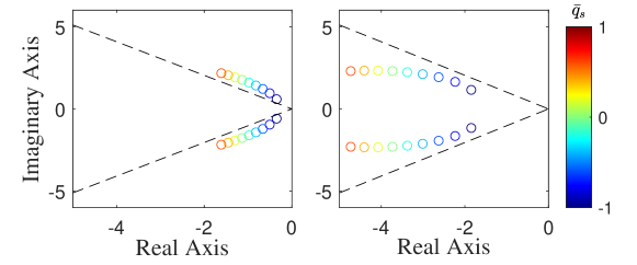
Figure 3: Open-loop (left) and closed-loop (right) poles when $\bar{q}_{s}$ changes from $-1$ to $1$ with an increment of $0.2$

It can be verified that Assumption 7 holds with the constants $L_{B}$, $L_{B^{\dagger}}$ and $L_{K_{x}}$ that can be computed numerically.

VI-B Uncertainties and adaptive controller design

We set the uncertainties in (1) as

$$\omega=0.7,\quad f(t,x)=[0.02\sin(20\pi x_{1}(t))+0.01\sin(\pi t),5x_{1}(t)x_{2}(t)+0.01\cos(2\pi t)]^{\top\!},$$ (129)

and $\Omega=[0.5,1.5]$. It is obvious that Assumption 3 holds, and furthermore, $f(t,x)$ satisfies the inequalities in Assumption 4 with a constant $b_{f}^{0}=0.01\sqrt{2}$. Using the Jacobian of $f(t,x)$ with respect to $x$ and the relation between the 2-norm and Frobenius norm of a matrix, one can verify that Assumption 5 holds with $L_{f}^{\delta}=0.16\pi^{2}+25\delta^{2}$. Additionally, Assumption 6 holds with the constant $l_{f}=0.0702$. So far we have verified that Assumptions 7, 3, 4, 5, 6 and 2 all hold.

For the robust adaptive controller design, we chose $\ T=0.001\ s,\ a=10,\ K=30,$ where $K$ specifies a nominal bandwidth of $30$ rad/s for the low-pass filter (see Remark 9). We used the gridding technique [4] to convert the PD-LMIs involved in the baseline and robust adaptive controller design into a finite number of LMIs, which were solved by Yalmip [49] and the Mosek solver [50]. For verification of the stability condition in (64), we need to compute the PPG bounds of $\mathcal{G}_{xm}(\theta)$, $\mathcal{G}_{xum}(\theta)$, and $\mathcal{H}_{xm}(\theta)\mathcal{C}K_{r}(\theta)$, using Lemma 5, and $\rho_{\textup{in}}$, using Lemma 3. Using an affine parameterization for the decision matrix $\mathrm{P}(\theta)$, we were able to obtain $\left\lVert\mathcal{G}_{xm}(\theta)\right\rVert_{\bar{\mathcal{L}}_{1}}=0.0509$ (with $\mu=3.7$), and $\left\lVert\mathcal{H}_{xm}(\theta)\mathcal{C}K_{r}(\theta)\right\rVert_{\bar{\mathcal{L}}_{1}}=6.35$ (with $\mu=3.2$). As mentioned in Remark 11, the weighting function, $\mathcal{W}(\theta)$, can be used to tune the trade-off between the performance of unmatched uncertainty attenuation (UUA) (represented by $\left\lVert\mathcal{G}_{um}(\theta)\right\rVert_{\bar{\mathcal{L}}_{1}}$) and the margin left for satisfying the stability condition in (64) (represented by $\left\lVert\mathcal{G}_{xum}(\theta)\right\rVert_{\bar{\mathcal{L}}_{1}}$). To focus on UUA, we selected $\mathcal{W}(\theta)=\textup{diag}(1,0)$, and obtained $\left\lVert\mathcal{G}_{xum}(\theta)\right\rVert_{\bar{\mathcal{L}}_{1}}=1.874$ (with $\mu=3.6$). Also, given the initial state bound $\left\lVert x_{0}\right\rVert\leq\rho_{0}=0.3$, we computed $\rho_{\textup{in}}=3.56$ using Lemma 3. With these bounds and the properties of $f(t,x)$ computed earlier, the stability condition (64) can be verified. As mentioned in Remark 20, the condition 64 could be rather conservative. Therefore, to better illustrate the capability of the proposed techniques to deal with large uncertainties, we did not enforce satisfaction of condition (64) (and Assumption 8) for the subsequent simulations.

VI-C Simulation results using the LPV plant

We first simulate the control system using the fitted LPV model introduced in Section VI-A. To verify the performance of the proposed controller under nonzero initialization error, i.e., $\tilde{x}(0)\neq 0$, we intentionally set $\hat{x}(0)=[\pi/180,-0.1]^{\top\!}$. The trajectories of the scheduling parameters were selected to be $\theta(t)=\sin(\frac{2\pi}{5}t)\times[0.5,1]^{\top\!}$. We tested the AOA tracking performance using three step reference signals of different magnitudes, denoted by $r_{1}(t),\ r_{2}(t)$ and $r_{3}(t)$, respectively. Considering the low bandwidth of the filter $\mathcal{C}(s)$, we chose not to filter the feedforward signal (see Remark 10). The state and control input trajectories are illustrated in Fig. 4 and Fig. 5, respectively. In Fig. 4, the ideal response given by the ideal dynamics in (4) is also included. One can see that the actual trajectories of $x_{1}$ (i.e., $\tilde{\alpha}$) were very close to their ideal counterparts and displayed scaled response under step references of different magnitude, despite the presence of the uncertainties in (129). Fig. 4 also shows a relatively large discrepancy between the actual trajectory of $x_{2}$ (i.e., $\tilde{q}$) and its ideal counterpart, as expected. This is because we considered mitigating the effect of unmatched uncertainty on $x_{1}$ only when designing the mapping ${\bar{\mathcal{H}}}(\theta)$.

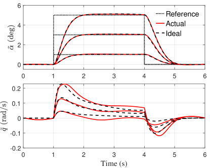
Figure 4: Trajectories of $x_{1}$ (top) and $x_{2}$ (bottom) under different references

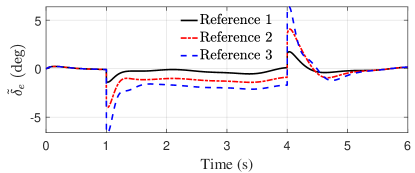
Figure 5: Trajectories of total control inputs under different references

Finally, Fig. 6 shows the actual lumped uncertainty and its estimation using the adaptive law in (44). We can see that due to the nonzero initialization error, i.e., $\tilde{x}(0)\neq 0$, the estimated uncertainty $\hat{\sigma}(t)$ deviated from its true value $\sigma(t,x,u)$ (defined in (42)) significantly at the first sampling interval $[0,T)$, but became very close to the true value afterward. This is consistent with Lemma 10.For comparison, Figure 7 depicts the performance degradation when we only applied the baseline input or compensated for the matched uncertainty only (by dropping the $\hat{\sigma}_{um}$ term in the control law defined by (46).

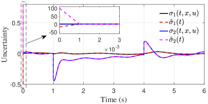
Figure 6: Actual and estimated (lumped) uncertainties under the step reference of two degrees. $\hat{\sigma}_{i}(t)$ and $\sigma_{i}(t,x,u)$ denote the $i$-th element of $\hat{\sigma}(t)$ and $\sigma(t,x,u)$, respectively.

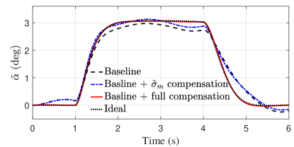
Figure 7: Trajectories of $x_{1}$ under $r(t)=3$ and different uncertainty compensation schemes

VI-D Simulation results using a full nonlinear model

We also used the full nonlinear model consisting of 13 states in [46] to perform more realistic simulations. We selected three trim points to represent the low, medium and high dynamic pressures:

• Low: $h=40,000\ \textup{ft}$, $V=400$ ft/s, $\bar{q}=48.5\ \textup{psf}$,

• Medium: $h=20,000\ \textup{ft}$, $\ V=600$ ft/s, $\bar{q}=228.6\ \textup{psf}$,

• High: $h=5,000\ \textup{ft},\$ $V=900$ ft/s, $\bar{q}=830.4\ \textup{psf}$.

We injected the same uncertainty in (129), and tested the tracking performance with a step reference signal. The AoA tracking performance is illustrated in Fig. 8, and the baseline and ${\mathcal{L}_{1}}$ control inputs are depicted in Fig. 9. From these results, we can see that the tracking response is different at different trim points, consistent with the design specifications. The actual trajectory of $x_{1}$ is still very close to its ideal counterpart, despite the presence of uncertainties and use of the simplified LPV model for controller design. For comparison, Fig. 10 depicts the significant degradation when there was no compensation for the uncertainties or compensation for the matched uncertainty only.

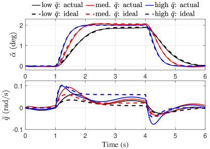
Figure 8: Trajectories of $x_{1}$ (top) and $x_{2}$ (right) under different trim points

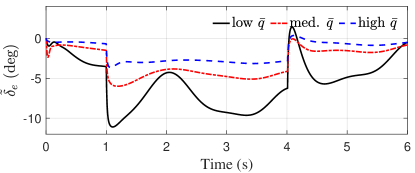
Figure 9: Trajectories of control inputs under different trim points

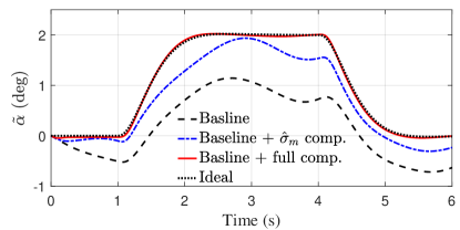
Figure 10: Trajectories of $x_{1}$ under the medium pressure scenario and different uncertainty compensation schemes

VII Conclusion

This paper presented a robust adaptive control architecture for LPV systems subject to unknown input gain and unmatched nonlinear uncertainties. Specifically, a new approach is introduced to mitigate the effect of the unmatched uncertainty on variables of interest, e.g., system outputs, which relies on computing a feedforward LPV mapping to minimize the peak-to-peak gain from the unmatched uncertainty to those variables of interest using linear matrix inequality (LMI) techniques. We derived the transient and steady-state performance bounds for the closed-loop system in terms of its input and output signals as compared to the same signals of a nominal system. Simulation results on the short-period dynamics of an F-16 aircraft validate theoretical development. Our future work includes extension to the output-feedback case.

Appendix A Proofs

A-A Proof of Lemma 1

Proof. For notation brevity, we define $\tilde{\omega}\triangleq\omega-\mathbb{I}_{m}$. Equation 14 directly follows from Assumption 4 and 11. Assumption 5 implies $\left\lVert f(t,x)-f(t,0)\right\rVert\leq L_{f}^{\delta}\left\lVert x\right\rVert\leq L_{f}^{\delta}\delta$, for any $\left\lVert x\right\rVert\leq\delta$ and any $t\geq 0$, which, together with Assumption 4, implies

$$\left\lVert f(t,x)\right\rVert\leq L_{f}^{\delta}\delta+b_{f}^{0},\quad\forall\left\lVert x\right\rVert\leq\delta,\forall t\geq 0.$$ (130)

With the bound $b_{\dot{\theta}}$ on $\left\lVert\dot{\theta}(t)\right\rVert$ in Assumption 1, we have

$$\left\lVert\theta(t_{1})-\theta(t_{2})\right\rVert=\left\|{\int_{{t_{1}}}^{{t_{2}}}{\dot{\theta}}(\tau)d\tau}\right\|\leq b_{\dot{\theta}}\left\lvert t_{1}-t_{2}\right\rvert.$$ (131)

Note that

$$\quad\left\|{B(\theta({t_{1}}))K_{x}(\theta({t_{1}})){x_{1}}\!-\!B(\theta({t_{2}}))K_{x}(\theta({t_{2}})){x_{2}}}\right\|$$

$$\leq\!\left\|{\left({B(\theta({t_{1}}))\!-\!B(\theta({t_{2}}))}\right)K_{x}(\theta({t_{1}})){x_{1}}}\right\|\!+\!\left\|{B(\theta({t_{2}}))\left({K_{x}(\theta({t_{1}}))\!-\!K_{x}(\theta({t_{2}}))}\right){x_{1}}}\right\|\!+\!\left\|{B(\theta({t_{2}}))K_{x}(\theta({t_{2}}))\left({{x_{1}}\!-\!{x_{2}}}\right)}\right\|$$

$$\leq\!L_{B}\left\|{\theta({t_{1}})\!-\!\theta({t_{2}})}\right\|\!\left\|{{x_{1}}}\right\|\left\|{K_{x}(\theta({t_{1}}))}\right\|\!+\!\left\|{B(\theta({t_{2}}))}\right\|{L_{K_{x}}}\left\|{\theta({t_{1}})\!-\!\theta({t_{2}})}\right\|\left\|{{x_{1}}}\right\|+\left\|{B(\theta({t_{2}}))K_{x}(\theta({t_{2}}))}\right\|\left\|{{x_{1}}\!-\!{x_{2}}}\right\|$$

$$\leq\!\left({L_{B}\left\|{K_{x}(\theta({t_{1}}))}\right\|\!+\!\left\|{B(\theta({t_{2}}))}\right\|{L_{K_{x}}}}\right)\!\left\|{{x_{1}}}\right\|b_{\dot{\theta}}\left\lvert t_{1}-t_{2}\right\rvert+\mathop{\max}\limits_{\theta\in\Theta}\left\|{B(\theta)K_{x}(\theta)}\right\|\left\|{{x_{1}}\!-\!{x_{2}}}\right\|$$

$$\leq\!\left({L_{B}b_{K_{x}}\!+\!b_{B}{L_{K_{x}}}}\right)\delta{b_{\dot{\theta}}}\left|{{t_{1}}\!-\!{t_{2}}}\right|\!+\!\mathop{\max}\limits_{\theta\in\Theta}\left\|{B(\theta)K_{x}(\theta)}\right\|\left\|{{x_{1}}\!-\!{x_{2}}}\right\|,$$

where the second inequality is due to Assumption 7 and 131, and the last inequality is due to the definitions in 13 and the fact that $\left\lVert x_{1}\right\rVert\leq\delta$. From the preceding inequality and the definition of ${{\bar{f}}}(t,x)$ in 11, we have

$$\left\|{{{\bar{f}}}({t_{1}},{x_{1}})-{{\bar{f}}}({t_{2}},{x_{2}})}\right\| \leq\left\|{f({t_{1}},{x_{1}})-f({t_{2}},{x_{2}})}\right\|+\left\|{\omega-{\mathbb{I}_{m}}}\right\|\left\|{B(\theta({t_{1}}))K_{x}(\theta({t_{1}})){x_{1}}-B(\theta({t_{2}}))K_{x}(\theta({t_{2}})){x_{2}}}\right\|$$

$$\leq{l_{f}}\left|t_{1}\!-\!t_{2}\right|+{L_{f}^{\delta}}\left\|{{x_{1}}-{x_{2}}}\right\|+\left\|{\omega-{\mathbb{I}_{m}}}\right\|\left({L_{B}b_{K_{x}}+b_{B}{L_{K_{x}}}}\right)\delta{b_{\dot{\theta}}}\left|t_{1}\!-\!t_{2}\right|$$

$$\quad+\left\|{\omega-{\mathbb{I}_{m}}}\right\|\mathop{\max}\limits_{\theta\in\Theta}\left\|{B(\theta)K_{x}(\theta)}\right\|\left\|{{x_{1}}-{x_{2}}}\right\|$$

$$\leq l_{{\bar{f}}}\left|t_{1}\!-\!t_{2}\right|+L_{{\bar{f}}}^{\delta}\left\|{{x_{1}}-{x_{2}}}\right\|.$$

Equation 11 implies

$$f_{1}(t,x) \!=\!B^{\dagger}\!(\theta){\bar{f}}(t,x)\!=\!B^{\dagger}\!(\theta)f(t,x)\!+\!(\omega\!-\!\mathbb{I}_{m})K_{x}(\theta)x,$$ (133a)

$$f_{2}(t,x) \!=\!B_{u}^{\dagger}(\theta)f(t,x),$$ (133b)

where $B^{\dagger}(\theta)$ and $B_{u}^{\dagger}(\theta)$ are the pseudo-inverse of $B(\theta)$ and $B_{u}(\theta)$, respectively. From Assumption 4 and 133, we obtain 15. On the other hand, from 133a, we have

$$\left\|{{f_{1}}({t_{1}},{x_{1}})\!-\!\!{f_{1}}({t_{1}},{x_{2}})}\right\| \leq\!\left\|{{B^{\dagger}}(\theta({t_{1}}))}\right\|\!\!\left\|{f({t_{1}},\!{x_{1}})\!-\!\!f({t_{1}},\!{x_{2}})}\right\|+\left\|{(\omega\!-\!{\mathbb{I}_{m}})K_{x}(\theta({t_{1}}))}\right\|\!\left\|{{x_{1}}\!\!-\!{x_{2}}}\right\|$$

$$\leq\!\left({{L_{f}^{\delta}}\left\|{{B^{\dagger}}(\theta({t_{1}}))}\right\|+\left\|{(\omega\!-\!{\mathbb{I}_{m}})K_{x}(\theta({t_{1}}))}\right\|}\right)\!\!\left\|{{x_{1}}\!-\!{x_{2}}}\right\|,$$

where the last inequality is due to Assumption 5. Considering the definition of $L_{f_{1}}^{\delta}$ in 18f, we have

$$\left\|{{f_{1}}({t_{1}},{x_{1}})\!-\!\!{f_{1}}({t_{1}},{x_{2}})}\right\|\leq L_{f_{1}}^{\delta}\!\left\|{{x_{1}}\!-\!{x_{2}}}\right\|.$$ (134)

Furthermore,

$$\left\|{{B^{\dagger}}(\theta({t_{1}}))f({t_{1}},{x_{2}})\!-\!{B^{\dagger}}(\theta({t_{2}}))f({t_{2}},{x_{2}})}\right\|$$

$$\leq \left\|{{B^{\dagger}}(\theta({t_{1}}))f({t_{1}},{x_{2}})\!-\!{B^{\dagger}}(\theta({t_{1}}))f({t_{2}},{x_{2}})}\right\|+\left\|{{B^{\dagger}}(\theta({t_{1}}))f({t_{2}},{x_{2}})\!-\!{B^{\dagger}}(\theta({t_{2}}))f({t_{2}},{x_{2}})}\right\|$$

$$\leq \left\|{{B^{\dagger}}(\theta({t_{1}}))}\right\|{l_{f}}\left|{{t_{1}}\!-\!{t_{2}}}\right|+L_{B^{\dagger}}b_{\dot{\theta}}\left|{{t_{1}}\!-\!{t_{2}}}\right|\!\left\|{f({t_{2}},{x_{2}})}\right\|$$ (135a)

$$\leq \left({{l_{f}}{\max_{\theta\in\Theta}}\left\|{{B^{\dagger}}(\theta)}\right\|+L_{B^{\dagger}}b_{\dot{\theta}}({b_{f}^{0}}+{L_{f}^{\delta}}\delta)}\right)\left|t_{1}\!-\!t_{2}\right|,$$ (135b)

where 135a is due to Assumption 6, 8 in Assumption 7 and 131, and 135b results from 130. As a result,

$$\left\|{{f_{1}}({t_{1}},{x_{2}})-{f_{1}}({t_{2}},{x_{2}})}\right\| =\left\|{B^{\dagger}}(\theta({t_{1}}))f({t_{1}},{x_{2}})\right.-{B^{\dagger}}(\theta({t_{2}}))f({t_{2}},{x_{2}})+\left.(\omega-{\mathbb{I}_{m}})\left({K_{x}(\theta({t_{1}}))-K_{x}(\theta({t_{2}}))}\right){x_{2}}\right\|$$

$$\leq\left\|{{B^{\dagger}}(\theta({t_{1}}))f({t_{1}},{x_{2}})-{B^{\dagger}}(\theta({t_{2}}))f({t_{2}},{x_{2}})}\right\|+\left\|{(\omega-{\mathbb{I}_{m}})}\right\|{L_{K_{x}}}b_{\dot{\theta}}\left|t_{1}\!-\!t_{2}\right|\left\|{{x_{2}}}\right\|,$$

where the inequality is due to 9 in Assumption 7 and 131. Further considering 135b and 18d, we have

$$\left\|{{f_{1}}({t_{1}},{x_{2}})-{f_{1}}({t_{2}},{x_{2}})}\right\|\leq~{}l_{f_{1}}\left|t_{1}\!-\!t_{2}\right|.$$ (136)

From 134 and 136, we obtain

$$\left\|{{f_{1}}({t_{1}},{x_{1}})-{f_{1}}({t_{2}},{x_{2}})}\right\|\leq\left\|{{f_{1}}({t_{1}},{x_{1}})-{f_{1}}({t_{1}},{x_{2}})}\right\|+\left\|{{f_{1}}({t_{1}},{x_{2}})-{f_{1}}({t_{2}},{x_{2}})}\right\|\leq L_{f_{1}}^{\delta}\left\|{{x_{1}}-{x_{2}}}\right\|+l_{f_{1}}\left|t_{1}\!-\!t_{2}\right|,$$ (137)

which proves 17 for $i=1$. Similarly,

$$\left\|{{f_{2}}({t_{1}},{x_{1}})\!-\!\!{f_{2}}({t_{1}},{x_{2}})}\right\| =\!\left\|{B_{u}^{\dagger}}(\theta({t_{1}}))\!\left({f({t_{1}},{x_{1}})\!\!-\!\!f({t_{1}},{x_{2}})}\right)\right\|$$

$$\leq\!\left\|{{B_{u}^{\dagger}}(\theta({t_{1}}))}\right\|\!\left\|{f({t_{1}},{x_{1}})\!-\!f({t_{1}},{x_{2}})}\right\|\!\leq\left\|{{B_{u}^{\dagger}}(\theta({t_{1}}))}\right\|{L_{f}^{\delta}}\left\|{{x_{1}}\!-\!{x_{2}}}\right\|\leq\!{L_{f_{2}}^{\delta}}\!\left\|{{x_{1}}\!-\!{x_{2}}}\right\|,$$ (138)

where the second last inequality is due to Assumption 5. Furthermore, following a procedure similar to that for deriving 135a, we can obtain

$$\left\|{{f_{2}}({t_{1}},{x_{2}})-{f_{2}}({t_{2}},{x_{2}})}\right\| =\left\|{{B_{u}^{\dagger}}(\theta({t_{1}}))f({t_{1}},{x_{2}})-{B_{u}^{\dagger}}(\theta({t_{2}}))f({t_{2}},{x_{2}})}\right\|$$

$$\leq\left\|{{B_{u}^{\dagger}}(\theta({t_{1}}))}\right\|{l_{f}}\left|t_{1}\!-\!t_{2}\right|+L_{B_{u}^{\dagger}}b_{\dot{\theta}}\left|t_{1}\!-\!t_{2}\right|\left\|{f({t_{2}},{x_{2}})}\right\|$$

$$\leq({{l_{f}}\left\|{{B_{u}^{\dagger}}(\theta({t_{1}}))}\right\|+L_{B_{u}^{\dagger}}b_{\dot{\theta}}\left\|{f({t_{2}},{x_{2}})}\right\|})\left|{{t_{1}}\!-\!{t_{2}}}\right|.$$

Further considering the definition of $l_{f_{2}}$ in 18e, we have

$$\left\|{{f_{2}}({t_{1}},{x_{2}})-{f_{2}}({t_{2}},{x_{2}})}\right\|\leq l_{f_{2}}\left|t_{1}\!-\!t_{2}\right|,$$ (139)

which, together with 138, leads to 17 for $i=2$. $\blacksquare$

A-B A Preliminary Lemma for Proof of Lemma 8

Lemma 13.

Consider the LPV generalized plant in (47), with parameter trajectories constrained by (2). There exists an LPV controller (48) enforcing internal stability and a bound $\gamma$ on the PPG of the closed-loop system, whenever there exist PD symmetric matrices $\tilde{X}(\theta)$ and $\tilde{Y}(\theta)$, a PD quadruple of state-space data ($\tilde{A}(\theta),\tilde{B}(\theta),\tilde{C}(\theta),\tilde{D}(\theta)$) and positive constants $\mu$ and $\upsilon$ such that the conditions (141) and (146) hold. In such case, the controller in (48) is given by

$$\left\{\begin{array}[]{rl}A_{\bar{\mathcal{H}}}(\theta)=&N^{-1}(\tilde{A}-\tilde{Y}{{\bar{B}}_{2}}{C_{\bar{\mathcal{H}}}}{M^{\top}}+\tilde{Y}\bar{A}\tilde{X}+\dot{\tilde{Y}}\tilde{X}+\dot{N}{M^{\top}})M^{-\top}\\ {B_{\bar{\mathcal{H}}}}(\theta)=&N^{-1}(\tilde{B}-\tilde{Y}{{\bar{B}}_{2}}{D_{\bar{\mathcal{H}}}})\\ C_{\bar{\mathcal{H}}}(\theta)=&\tilde{C}M^{-\top}\\ {D_{\bar{\mathcal{H}}}}(\theta)=&\tilde{D},\end{array}\right.$$ (140)

where $M$ and $N$ are computed from the factorization $N(\theta)M(\theta)^{\top\!}=\mathbb{I}_{\bar{n}}-\tilde{X}(\theta)\tilde{Y}(\theta)\mathrel{\mathop{\mathchar 58\relax}}$

$$\left[{\begin{array}[]{*{20}{c}}{\!-\dot{\tilde{X}}\!+\!\langle{\bar{A}\tilde{X}\!+\!{{\bar{B}}_{2}}\tilde{C}}\rangle\!+\!\mu\tilde{X}}&\star&\star\\ {\tilde{A}\!+\!{\bar{A}^{\top}}\!+\!\mu{\mathbb{I}_{\bar{n}}}}&{-\dot{\tilde{Y}}\!+\!\langle{\bar{A}\tilde{Y}}\rangle\!+\!\mu\tilde{Y}}&\star\\ {{{({{\bar{B}}_{1}}\!+\!{{\bar{B}}_{2}}\tilde{D}{{\bar{D}}_{21}})}^{\top}}}&\!{\bar{B}}_{1}^{\top}\!\!+\!\bar{D}_{21}^{\top\!}({{\tilde{B}}^{\top}}\!\!+\!\tilde{D}{\bar{B}}_{2}^{\top\!})&{-\upsilon{\mathbb{I}_{n-m}}}\end{array}}\right]<0,$$ (141)

$$\vspace{-2mm}\left[{\begin{array}[]{*{20}{c}}{\mu\tilde{X}}&\star&\star&\star\\ {\mu{\mathbb{I}_{\bar{n}}}}&{\mu\tilde{Y}}&\star&\star\\ 0&0&{(\gamma-\upsilon){\mathbb{I}_{n-m}}}&\star\\ {{{\bar{C}}_{1}}\tilde{X}\!+\!{{\bar{D}}_{12}}\tilde{C}}&{{{\bar{C}}_{1}}}&{{{\bar{D}}_{11}}\!+\!{{\bar{D}}_{12}}\tilde{D}{{\bar{D}}_{21}}}&{\gamma{\mathbb{I}_{n}}}\end{array}}\right]>0.$$ (146)

Note that in 140, 141 and 146, the dependence of the decision matrices on $\theta$ is omitted for brevity.

Sketch of proof. The result directly follows from extension of the conditions for bounding the PPG of LTI systems [40, Section IV.E] to LPV systems, and consideration of the fact that $\bar{C}_{2}=0$ and $\bar{D}_{11}=0$ according to (47). The extension is achieved through the use of a PD Lyapunov function that depends on $\tilde{X}$ and $\tilde{Y}$. $\blacksquare$

Remark 24.

Due to the derivative terms, $\dot{\tilde{Y}}(\theta)$ and $\dot{\tilde{N}}(\theta)$, in (140), implementation of the controller needs the derivative of scheduling parameters, $\dot{\theta}$, which is often not available in practice. One way to remove the dependence on $\dot{\theta}$ is to impose structures on the Lyapunov matrices , i.e., making either $\tilde{X}$ or $\tilde{Y}$ parameter-independent [4, Section III]. However, enforcing this structure will induce conservatism. Motivated by the idea in [44], we derive new conditions equivalent to (141) and (146) while removing the use of $\dot{\theta}$ in controller implementation without resorting to structured Lyapunov functions. The new conditions are given in Lemma 8.

Appendix B State-Space Realizations of LPV Mappings

We now show the state-space realization of mappings $\mathcal{G}_{xm}(\theta)$ and $\mathcal{H}_{xm}(\theta)\mathcal{C}K_{r}(\theta)$ involved in the stability condition in (64). The mapping $\mathcal{H}_{xm}(\theta)$ defined for 37 can be rewritten using its state-space realization as $\left[\begin{array}[]{c|c}A_{m}(\theta)&B(\theta)\\ \hline\cr\mathbb{I}_{n}&0_{n\times m}\end{array}\right]$. The mappings $\mathcal{C}$ for the filter in (36) and $\mathbb{I}_{m}-\mathcal{C}$ can be written as $\left[\begin{array}[]{c|c}-\omega K&\mathbb{I}_{m}\\ \hline\cr\omega K&0_{m\times m}\end{array}\right]$ and $\left[\begin{array}[]{c|c}-\omega K&\mathbb{I}_{m}\\ \hline\cr-\omega K&\mathbb{I}_{m}\end{array}\right]$, respectively. Thus, the definition in (39a) implies that $\mathcal{G}_{xm}(\theta)$ can be represented as

$$\mathcal{G}_{xm}(\theta)=\left[\begin{array}[]{c|c}\begin{bmatrix}A_{m}(\theta)&-B(\theta)\omega K\\ 0_{m\times n}&-\omega K\end{bmatrix}&\begin{bmatrix}B(\theta)\\ \mathbb{I}_{m}\end{bmatrix}\\ \hline\cr\begin{bmatrix}\mathbb{I}_{n}&0_{n\times m}\end{bmatrix}&0_{n\times m}\end{array}\right].$$ (147)

Similarly, the mapping $\mathcal{H}_{xm}(\theta)\mathcal{C}K_{r}(\theta)$ can be written as

$$\mathcal{H}_{xm}(\theta)\mathcal{C}K_{r}(\theta)\!=\!\left[\begin{array}[]{c|c}\begin{bmatrix}A_{m}(\theta)&B(\theta)\omega K\\ 0_{m\times n}&-\omega K\end{bmatrix}&\begin{bmatrix}0_{n\times m}\\ K_{r}(\theta)\end{bmatrix}\\ \hline\cr\begin{bmatrix}\mathbb{I}_{n}&0_{n\times m}\end{bmatrix}&0_{m\times m}\end{array}\right].$$ (148)

Note that the state space matrices in 147 and 148 are affine with respect to $\omega$. Similarly, the state-space realization of the mapping $\mathcal{G}_{xum}(\theta)$ can be derived and shown to have an affine relation with respect to $\omega$. With these state space realizations, the PPG bounds of $\mathcal{G}_{xm}(\theta)$, $\mathcal{H}_{xm}(\theta)\mathcal{C}K_{r}(\theta)$, and $\mathcal{G}_{xum}(\theta)$ can be computed using Lemma 5 in order to verify the stability condition in (64). See Section IV-C for an explanation of how to deal with the uncertain $\omega$ in computing the PPG bounds.

References

• [1] Wilson J Rugh and Jeff S Shamma. Research on gain scheduling. Automatica, 36(10):1401–1425, 2000. https://doi.org/10.1016/S0005-1098(00)00058-3.
• [2] Jeff S Shamma and Michael Athans. Guaranteed properties of gain scheduled control for linear parameter-varying plants. Automatica, 27(3):559–564, 1991. https://doi.org/10.1016/0005-1098(91)90116-J.
• [3] Fen Wu, Xin Hua Yang, Andy Packard, and Greg Becker. Induced ${L}_{2}$-norm control for LPV system with bounded parameter variation rates. Int. J. Robust Nonlinear Control, 6(9-10):983–998, 1996. https://doi.org/10.1002/(SICI)1099-1239(199611)6:9/10%3C983::AID-RNC263%3E3.0.CO;2-C.
• [4] Pierre Apkarian and Richard J Adams. Advanced gain-scheduling techniques for uncertain systems. IEEE Trans. Control Syst. Technol., 6(1):21–32, 1998. https://doi.org/10.1109/ACC.1997.612082.
• [5] Masayuki Sato. Gain-scheduled output-feedback controllers depending solely on scheduling parameters via parameter-dependent Lyapunov functions. Automatica, 47(12):2786–2790, 2011. https://doi.org/10.1016/j.automatica.2011.09.023.
• [6] Jean-Marc Biannic, Pierre Apkarian, and William L Garrard. Parameter varying control of a high-performance aircraft. J Guid Control Dyn, 20(2):225–231, 1997. https://doi.org/10.2514/2.4045.
• [7] Bei Lu, Fen Wu, and SungWan Kim. Switching LPV control of an F-16 aircraft via controller state reset. IEEE Trans. Control Syst. Technol., 14(2):267–277, 2006. https://doi.org/10.1109/TCST.2005.863656.
• [8] Tianyi He, Ali K. Al-Jiboory, Guoming G. Zhu, Sean S.-M. Swei, and Weihua Su. Application of ICC LPV control to a blended-wing-body airplane with guaranteed $H_{\infty}$ performance. Aerospace Science and Technology, 81:88–98, 2018. https://doi.org/10.1016/j.ast.2018.07.046.
• [9] Tianyi He, Guoming G Zhu, Sean S-M Swei, and Weihua Su. Smooth-switching lpv control for vibration suppression of a flexible airplane wing. Aerospace Science and Technology, 84:895–903, 2019. https://doi.org/10.1016/j.ast.2018.11.029.
• [10] Xiukun Wei and Luigi Del Re. Gain scheduled $H_{\infty}$ control for air path systems of diesel engines using LPV techniques. IEEE Trans. Control Syst. Technol., 15(3):406–415, 2007. https://doi.org/10.1109/TCST.2007.894633.
• [11] Andrew White, Guoming Zhu, and Jongeun Choi. Hardware-in-the-loop simulation of robust gain-scheduling control of port-fuel-injection processes. IEEE Trans. Control Syst. Technol., 19(6):1433–1443, 2011. https://doi.org/10.1109/TCST.2010.2095420.
• [12] Petros A. Ioannou and Jing Sun. Robust Adaptive Control. Dover Publications, Inc., Mineola, NY, 2012.
• [13] Kumpati S. Narendra and Anuradha M. Annaswamy. Stable Adaptive Systems. Prentice Hall, Englewood Cliffs, NJ, 1989.
• [14] Eugene Lavretsky and Kevin Wise. Robust and Adaptive Control: With Aerospace Applications. Springer, 2012.
• [15] J. Han. From PID to active disturbance rejection control. IEEE Trans. Ind. Electron., 56(3):900–906, 2009.
• [16] Wen-Hua Chen, Jun Yang, Lei Guo, and Shihua Li. Disturbance-observer-based control and related methods—An overview. IEEE Trans. Ind. Electron., 63(2):1083–1095, 2015. https://doi.org/10.1109/TIE.2015.2478397.
• [17] Naira Hovakimyan and Chengyu Cao. $\mathcal{L}_{1}$ Adaptive Control Theory: Guaranteed Robustness with Fast Adaptation. Society for Industrial and Applied Mathematics, Philadelphia, PA, 2010.
• [18] Naira Hovakimyan, Chengyu Cao, Evgeny Kharisov, Enric Xargay, and Irene Gregory. $\mathcal{L}_{1}$ adaptive control for safety critical systems. IEEE Control Systems Magazine, 55:54–104, October 2011. https://doi.org/10.1109/MCS.2011.941961.
• [19] Kasey A. Ackerman, Enric Xargay, Ronald Choe, Naira Hovakimyan, M. Christopher Cotting, Robert B. Jeffrey, Margaret P. Blackstun, T. Paul Fulkerson, Timothy R. Lau, and Shawn S. Stephens. Evaluation of an $\mathcal{L}_{1}$ adaptive flight control law on Calspan’s variable-stability Learjet. J Guid Control Dyn, 40(4):1051–1060, 2017. https://doi.org/10.2514/1.G001730.
• [20] Kasey Ackerman, Javier Puig-Navarro, Naira Hovakimyan, M. Christopher Cotting, Dustin J. Duke, Miguel J. Carrera, Nathan C. McCaskey, Dario Esposito, Jessica M. Peterson, and Jonathan R. Tellefsen. Recovery of desired flying characteristics with an $\mathcal{L}_{1}$ adaptive control law: Flight test results on Calspan’s VSS Learjet. In AIAA SciTech 2019 Forum, San Diego, California, January 2019. AIAA 2019-1084. https://doi.org/10.2514/6.2019-1084.
• [21] Steven Snyder, Pan Zhao, and Naira Hovakimyan. $\mathcal{L}_{1}$ adaptive control with switched reference models: Application to Learn-to-Fly. Journal of Guidance, Control, and Dynamics, 45(12):2229––2242, 2022. https://doi.org/10.2514/1.G006305.
• [22] Xiaofeng Wang and Naira Hovakimyan. $\mathcal{L}_{1}$ adaptive controller for nonlinear time-varying reference systems. Systems & Control Letters, 61(4):455 – 463, 2012. https://doi.org/10.1016/j.sysconle.2012.01.010.
• [23] Brett T Lopez and Jean-Jacques E Slotine. Adaptive nonlinear control with contraction metrics. IEEE Control Systems Letters, 5(1):205–210, 2020. https://doi.org/10.1109/LCSYS.2020.3000190.
• [24] Arun Lakshmanan, Aditya Gahlawat, and Naira Hovakimyan. Safe feedback motion planning: A contraction theory and $\mathcal{L}_{1}$-adaptive control based approach. In Proceedings of 59th IEEE Conference on Decision and Control (CDC), pages 1578–1583, 2020. https://doi.org/10.1109/CDC42340.2020.9303957.
• [25] Pan Zhao, Ziyao Guo, and Naira Hovakimyan. Robust nonlinear tracking control with exponential convergence using contraction metrics and disturbance estimation. Sensors, 22(13):4743, 2022. https://doi.org/10.3390/s22134743.
• [26] Jing Xie and Jun Zhao. Model reference adaptive control for switched LPV systems and its application. IET Control Theory & Applications, 10(17):2204–2212, 2016. https://doi.org/10.1049/iet-cta.2015.1332.
• [27] Steven Snyder, Pan Zhao, and Naira Hovakimyan. Adaptive control for linear parameter-varying systems with application to a VTOL aircraft. Aerospace Science and Technology, 112:106621, 2021. https://doi.org/10.1016/j.ast.2021.106621.
• [28] Enric Xargay, Naira Hovakimyan, and Chengyu Cao. $\mathcal{L}_{1}$ adaptive controller for multi-input multi-output systems in the presence of nonlinear unmatched uncertainties. In Proc. ACC, pages 874–879, 2010. https://doi.org/10.1109/ACC.2010.5530686.
• [29] S. Li, J. Yang, W. Chen, and X. Chen. Generalized extended state observer based control for systems with mismatched uncertainties. IEEE Trans. Ind. Electron., 59(12):4792–4802, 2012. https://doi.org/10.1109/TIE.2011.2182011.
• [30] Jun Yang, Shihua Li, and Wen-Hua Chen. Nonlinear disturbance observer-based control for multi-input multi-output nonlinear systems subject to mismatching condition. Int. J. Control, 85(8):1071–1082, 2012. https://doi.org/10.1080/00207179.2012.675520.
• [31] Xinjiang Wei and Lei Guo. Composite disturbance-observer-based control and $H_{\infty}$ control for complex continuous models. Int. J. Robust Nonlinear Control, 20(1):106–118, 2010. https://doi.org/10.1109/WCICA.2008.4593684.
• [32] Bin Yao and Masayoshi Tomizuka. Adaptive robust control of SISO nonlinear systems in a semi-strict feedback form. Automatica, 33(5):893–900, 1997. https://doi.org/10.1016/S0005-1098(96)00222-1.
• [33] Ali J. Koshkouei, Alan S. I. Zinober, and Keith J. Burnham. Adaptive sliding mode backstepping control of nonlinear systems with unmatched uncertainty. Asian Journal of Control, 6(4):447–453, 2004. https://doi.org/10.1111/j.1934-6093.2004.tb00365.x.
• [34] Haibin Sun, Shihua Li, Jun Yang, and Wei Xing Zheng. Global output regulation for strict-feedback nonlinear systems with mismatched nonvanishing disturbances. Int. J. Robust Nonlinear Control, 25(15):2631–2645, 2015. https://doi.org/10.1002/rnc.3216.
• [35] Metehan Yayla and Ali Turker Kutay. Adaptive control algorithm for linear systems with matched and unmatched uncertainties. In IEEE Conference on Decision and Control, pages 2975–2980, 2016. https://doi.org/10.1109/CDC.2016.7798713.
• [36] Girish Joshi and Girish Chowdhary. Hybrid direct-indirect adaptive control of nonlinear system with unmatched uncertainty. In International Conference on Control, Decision and Information Technologies (CoDIT), pages 127–132, 2019. https://doi.org/10.1109/CoDIT.2019.8820301.
• [37] Pierre Apkarian, Pascal Gahinet, and Greg Becker. Self-scheduled ${H}_{\infty}$ control of linear parameter-varying systems: A design example. Automatica, 31(9):1251–1261, 1995. https://doi.org/10.1016/0005-1098(95)00038-X.
• [38] Javad Mohammadpour and Carsten W Scherer. Control of Linear Parameter Varying Systems with Applications. Springer Science & Business Media, 2012.
• [39] Eugene Lavretsky, Ross Gadient, and Irene M Gregory. Predictor-based model reference adaptive control. J Guid Control Dyn, 33(4):1195–1201, 2010. https://doi.org/10.1109/CCDC52312.2021.9601487.
• [40] Carsten Scherer, Pascal Gahinet, and Mahmoud Chilali. Multiobjective output-feedback control via LMI optimization. IEEE Trans. Autom. Control, 42(7):896–911, 1997. https://doi.org/10.1109/9.599969.
• [41] Sungyung Lim. Analysis and Control of Linear Parameter-Varying Systems. PhD thesis, Stanford University, 1998.
• [42] Shihua Li, Haibin Sun, Jun Yang, and Xinghuo Yu. Continuous finite-time output regulation for disturbed systems under mismatching condition. IEEE Trans. Autom. Control, 60(1):277–282, 2014. https://doi.org/10.1109/TAC.2014.2324212.
• [43] Jiaxing Che and Chengyu Cao. $\mathcal{L}_{1}$ adaptive control of system with unmatched disturbance by using eigenvalue assignment method. In IEEE Conference on Decision and Control, pages 4823–4828, 2012. https://doi.org/10.1109/CDC.2012.6426412.
• [44] Masayuki Sato. Inverse system design for LPV systems using parameter-dependent Lyapunov functions. Automatica, 44(4):1072–1077, 2008. https://doi.org/10.1016/j.automatica.2007.08.013.
• [45] Didier Henrion and Andrea Garulli. Positive Polynomials in Control, volume 312 of Lecture Notes in Control and Information Sciences. Springer Verlag., Berlin, 2005.
• [46] Ying Huo. Matlab software package for six degrees of freedom nonlinear F-16 aicraft model. https://archive.siam.org/books/dc11/, 2006.
• [47] K.A. Wise, E. Lavretsky, and N. Hovakimyan. Adaptive control of flight: theory, applications, and open problems. In Proc. ACC, pages 5966–5971, 2006. https://doi.org/10.1109/ACC.2006.1657677.
• [48] Mahmoud Chilali and Pascal Gahinet. $H_{\infty}$ design with pole placement constraints: An LMI approach. IEEE Trans. Autom. Control, 41(3):358–367, 1996. https://doi.org/10.1109/9.486637.
• [49] Johan Lofberg. YALMIP: A toolbox for modeling and optimization in MATLAB. In Proceedings of 2004 IEEE International Symposium on Computer Aided Control Systems Design, pages 284–289, 2004. https://doi.org/10.1109/CACSD.2004.1393890.
• [50] Erling D. Andersen and Knud D. Andersen. The MOSEK interior point optimizer for linear programming: An implementation of the homogeneous algorithm. In High Performance Optimization, pages 197–232. 2000.