An Angular Multigrid Preconditioner for the Radiation Transport Equation with Forward-Peaked Scatter

Abstract

In a previous paper (Lathouwers and Perkó, 2019) we have developed an efficient angular multigrid preconditioner for the Boltzmann transport equation with forward-peaked scatter modeled by the Fokker-Planck approximation. The discretization was based on a completely discontinuous Galerkin finite element scheme both for space and angle. The scheme was found to be highly effective on isotropically and anisotropically refined angular meshes. The purpose of this paper is to extend the method to non-Fokker-Planck models describing the forward scatter by general Legendre expansions. As smoother the standard source iteration is used whereas solution on the coarsest angular mesh is effected by a special sweep procedure that is able to solve this problem with highly anisotropic scatter using only a small number of iterations. An efficient scheme is obtained by lowering the scatter order in the multigrid preconditioner. A set of test problems is presented to illustrate the effectivity of the method, i.e. in less iterations than the single-mesh case and more importantly with reduced computational effort.

1 Introduction

The solution of the linear Boltzmann equation (LBE) is computationally expensive due to its high dimensionality. Studies of numerical techniques focus mostly on the steady mono-energetic form being the building block for more complex cases. Discretization is generally performed by discrete ordinates which is straightforward to implement. Spatial discretization is most often performed by the discontinous Galerkin in space. Whatever the discretization used, some form of iteration is needed to resolve the system of equations. Source iteration, the most widespread technique, works well for optically thin media but is less suitable for thick scattering materials. As the slowest mode of convergence in thick scattering media has little angular dependence this can be remedied by the diffusion synthetic acceleration (DSA) that accelerates reduction of these errors by solution of a diffusion problem. When used as preconditioner in a Krylov method, this practically gives rise to an unconditionally effective and stable method.

For anisotropic scattering and in thin media, DSA is still ineffective. Multigrid methods where the problem is formulated on multiple levels lead to a more successfull approach. The basic principle of the multigrid approach is to smooth small wavelength errors on successive grids combined with an exact solver on the coarsest grid. DSA can be viewed as a two-grid technique in physical approach, switching between complete transport on the fine level and diffusion on the coarse level.

Our previous paper [6] has an extensive discussion of literature on multigrid approaches which we only briefly summarize here. The multigrid technique for radiation transport problems was pioneered by Morel and Manteuffel [9] where they constructed an angular multigrid method for the one dimensional $S_{N}$ equations. The method was extended to two dimensions by Pautz [11] by the introduction of high-frequency filtering to increase stability of the method. Various references have investigated the efficiency of angular multigrid schemes for both the $P_{N}$ and the $S_{N}$ equations [7, 8, 1, 12, 2]. These papers have shown the great benefit of multigrid: speedups of up to 10 are reported compared to single grid methods.

In previous work we have introduced a novel finite element angular discretization of the transport equation [5]. The method offers the capability to anisotropically refine the sphere to focus on important directions. In a later paper we added a discretization scheme for the Fokker-Planck small angle scatter term [4] and an angular multigrid scheme for the efficient solution [6]. The scheme utilizes the multigrid method as preconditioner for a Krylov method and was found to be highly effective compared to the single mesh preconditioner. The purpose of this paper is to widen the scope of these previously introduced methods to the more general case of highly anisotropic scatter as modeled by Legendre scatter expansion.

This paper is outlined as follows. In Section 2, we summarize the discontinuous Galerkin discretization in space-angle that our method is based on. The standard source iteration procedure is described in Section 3. The angular multigrid procedure proposed in the present work is discussed in Section 4 comprising of the mesh hierarchy, and the inter-grid transfers. Section 5 describes a newly formulated sweep methodology for efficient coarse mesh solution compatible with high order scatter. The method is tested on a set of model problems. Final conclusions are drawn in Section 6.

2 Space-angle discretization of the transport equation

The space-angle discretization of the Boltzmann equation has been presented in detail in [5] and [4], and will therefore be described briefly by only covering the essentials. Details can be found in the original references. Particle transport with highly anisotropic scatter is described by the linear Boltzmann transport equation. We neglect energy dependence in this paper as the focus is on accelerating the single group iterative method. The linear mono-energetic Boltzmann equation reads

$$\mathbf{\Omega}\cdot\nabla\phi(\textbf{r},\mathbf{\Omega})+\Sigma_{t}(\textbf{r})\phi(\textbf{r},\mathbf{\Omega})=Q(\textbf{r},\mathbf{\Omega})$$ (1)

where r is the spatial coordinate, $\mathbf{\Omega}$ is the unit direction vector, $\phi$ is the angular flux density, $Q$ is the volumetric source density including scatter, $\Sigma_{t}$ is the total macroscopic cross section. The angular flux for incoming directions is specified on the domain boundary, $\Gamma_{I}$,

$$\phi(\textbf{r},\mathbf{\Omega})=\phi_{in}(\textbf{r},\mathbf{\Omega}),\;\textbf{r}\in\Gamma_{I},\;\mathbf{\Omega}\cdot\hat{\textbf{n}}<0$$ (2)

2.1 Phase space elements

The spatial domain $V$ is made up of elements $V_{k}$, where $k$ is the index of the spatial element. A discontinuous solution space $S_{h,p}$, is defined containing polynomials of order $p$ at most. This is a standard approach and we focus our attention on the angular discretization.

The construction of angular elements is based on hierarchical sectioning of the unit sphere into patches, $D_{p}$, where $p$ is the patch index. The coordinate planes divide the sphere into cardinal octants, which are spherical triangles. We also assign a level, $l_{p}$, to a patch. The spherical triangles at the coarsest level are assigned a level of $l_{p}=0$. Spherical triangles with $l_{p}=1$ are obtained by halving the edges of the $l_{p}=0$ patches and subsequently connecting the emerged points with great circles. Every patch is hereby split into four daughters. This procedure can be repeated to arbitrary depth and locally on the sphere (aniostropic refinement).

The angular subdivision of the sphere is described by a set $P$ of patch indices such that $\cup_{p\in P}D_{p}\equiv D$ where $D$ denotes the unit sphere surface and $D_{p}\cap D_{q}\equiv\emptyset$ for $\forall p,q\in P,p\neq q$. The phase space mesh is then obtained by assigning an angular subdivision $P_{k}$ to each spatial element $V_{k}$ providing a high level of flexibility.

2.2 Angular basis functions

Two sets of angular basis functions, $\psi_{[p]d}(\mathbf{\Omega})$, are used throughout this paper. Both are local to the patch $D_{p}$ by setting $\psi_{[p]d}(\mathbf{\Omega})=0$ if $\mathbf{\Omega}\notin D_{p}$ and are discontinuous at the patch boundary. Here $\psi_{[p]d}(\mathbf{\Omega})$ denotes the $d$-th basis function on the patch with index $p$. The locality-property of the functions ensures that the streaming-removal terms will not couple to non-overlapping patches. As explained later, this eases the use of sweep-based algorithm. The two basis functions sets are:

1. Const A unit value function on the patch.

2. Lin A nodal set of three functions satisfying $\psi_{[p]d}(\mathbf{\Omega}_{d^{\prime}})=\delta_{dd^{\prime}}$ where $\mathbf{\Omega}_{d^{\prime}}$ are the patch-vertices. These functions result from projecting the standard Lagrange functions on a specific flat triangle on the octahedron onto the sphere. The flat triangle is formed by projecting the vertices of the patch to the octahedron.

2.3 Discretization

The flux in each energy group is written as a product of spatial and angular basis functions as

$$\phi(\textbf{r},\mathbf{\Omega})=\sum_{k,i}\sum_{p\in P_{k},d}\phi\indices{{}_{[k,p]}^{i,d}}\Phi_{[k]i}(\textbf{r})\Psi_{[p]d}(\mathbf{\Omega})$$ (3)

where $\Phi_{[k]i}(\textbf{r})$ is the $i$-th spatial basis function of element $k$ and $\Psi_{[p]d}(\mathbf{\Omega})$ is the $d$-th angular basis function on patch (angular element) $p$.

Substituting the expansion given by eq:Expansioneq: eq:Expansioneq:[] sec:eq: sec:eq:[] Equation LABEL:eq:\RefResult into the transport equation (LBEeq: LBEeq:[] sec:eq: sec:eq:[] Equation LABEL:eq:\RefResult), multiplying with a test function in space and angle and subsequently integrating over complete phase space leads to:

$$\sum_{f}\Upsilon_{[f,j,q]lm}-\sum_{\xi=1}^{3}\sum_{i}\sum_{d}V_{[j]li\xi}\phi\indices{{}_{[j,q]}^{id}}A\indices{{}_{[q,p]md}^{\xi}}+\Sigma_{a}\sum_{i}\sum_{d}N_{[j]li}\phi\indices{{}_{[j,q]}^{id}}M_{[q]md}=Q_{[j,q]lm},$$ (4)

where the streaming term reads

$$\Upsilon_{[f,j,q]lm}=\int_{\partial V_{j}^{f}}\Phi_{[j]l}(\textbf{r})\sum_{\begin{array}[]{c}k\in\{j,j_{f}^{\prime}\}\\ i\end{array}}\sum_{\begin{array}[]{c}p\in P_{k}\\ d\end{array}}\phi\indices{{}_{[k,p]}^{id}}\Phi_{[k]i}(\textbf{r})A_{[f,q,p]md}d\textbf{r}$$ (5)

and we made use of the following shorthand notations:

$$N_{[j]li}=\int_{V_{j}}\Phi_{[j]l}(\textbf{r})\Phi_{[j]i}(\textbf{r})d\textbf{r}$$ (6)

$$V_{[j]li\xi}=\int_{V_{j}}\nabla_{\xi}\Phi_{[j]l}(\textbf{r})\Phi_{[j]i}(\textbf{r})d\textbf{r}$$ (7)

$$A\indices{{}_{[q,p]md}^{\xi}}=\int_{D_{q}}\Omega^{\xi}\Psi_{[q]m}(\mathbf{\Omega})\Psi_{[p]d}(\mathbf{\Omega})d\mathbf{\Omega}$$ (8)

$$A_{[f,q,p]md}=\sum_{\xi=1}^{3}{\hat{n}}_{[f]\xi}A\indices{{}_{[q,p]md}^{\xi}}$$ (9)

$$A_{[f,q]md}=A_{[f,q,q]md}$$ (10)

$$M_{[q,p]md}=\int_{D_{q}}\Psi_{[q]m}(\mathbf{\Omega})\Psi_{[q]d}(\mathbf{\Omega})d\mathbf{\Omega}$$ (11)

$$M_{[q]md}=M_{[q,q]md}$$ (12)

$$Q_{[j,q]lm}=\int_{V_{j}}\int_{D_{q}}\Phi_{[j]l}(\textbf{r})\Psi_{[q]m}(\mathbf{\Omega})Q(\textbf{r},\mathbf{\Omega})d\mathbf{\Omega}d\textbf{r}.$$ (13)

Here, element $j$ has faces indexed by $f$ with its neighbor at face $f$ denoted as $j_{f}^{\prime}$ and ${\hat{n}}_{[f]\xi}$ is the $\xi$ coordinate of the outward normal of face $f$ in element $j$. The mass matrices in space and angle are denoted by $N$ and $M$, respectively. $V$ contains the volmetric streaming integral and $A$ is the angular Jacobian.

The face integrals from streaming need to be made unique by an upwinding procedure. In $S_{N}$ schemes this is straightforward. Here, the angular components on a patch need to be treated simultaneously. Various authors (e.g. [10]) have introduced Riemann procedures to separate the surface terms into inward and outward contributions. In previous papers [5, 4] we have derived how the numerical flux needs to be evaluated in the different situations, i.e. where the neighbor is either (i) equally refined, (ii) coarser or (iii) finer. To prevent repetition and concentrate on the multigrid aspects, we refer the reader to the original references for more in-depth discussion.

3 Single-grid solution approach

The discrete transport equation is written as

$$L{\boldsymbol{\phi}}=S{\boldsymbol{\phi}}+{\bf f}.$$ (14)

Here, $L$ and $S$ are the discrete transport and scatter operators, respectively and $f$ is the vector containing the independent source.

We use preconditioned Bicgstab [13] to solve the linear system with $L^{-1}$ as preconditioner, corresponding to Krylov-accelerated source iteration

$$L{\boldsymbol{\phi}}^{k+1}=S{\boldsymbol{\phi}}^{k}+{\boldsymbol{f}}.$$ (15)

In discrete ordinates codes the operator $L^{-1}$ is easily applied as the ordinates are independent. Here, we use a finite element discretization in angle, where such a sweep is no longer exact. The cause is possible bi-directionality due to some directions on a patch being incoming whereas others are outgoing with respect to the face. To precondition the system we have devised the following sweep algorithm:

• An $S_{2}$ ordinate set is used and for each ordinate, corresponding to a particular octant, the sweep order of the elements is determined.

• For each direction, we traverse the spatial elements and each angular element in the octant is visited and the corresponding linear system is solved. In more mathematical terms we perform a block Gauss-Seidel iteration for a given ordering of the spatio-angular elements. Splitting $L$ into implicit and explicit part, $L=L_{I}+L_{E}$, the iteration reads

  $$L_{I}{\bf\phi}^{k+1}=(S-L_{E}){\bf\phi}^{k}+{\bf f}$$ (16)

  and the preconditioner then is $L_{I}$.

We have previously demonstrated that this sweep algorithm is an effective preconditioner (see [5] for more details). In problems where scatter is highly anisotropic the procedure unfortunately becomes less effective.

4 An angular multigrid preconditioner

The multigrid method smooths the error on a given mesh and then transfers the residual to a coarser mesh where the lower frequency errors can be more effectively attenuated. As we deal with a linear problem, we use the linear multigrid algorithm as shown in Figure 1.

Algorithm $LMG(\boldsymbol{\phi}_{l},{\bf{f}}_{l},l)$
if $(l=0)$ then
$S(\boldsymbol{\phi}_{l},{\bf{f}}_{l},\nu_{coarse})$
else
$S(\boldsymbol{\phi},f,\nu_{pre})$
${\bf{r}}_{l}={\bf{f}}_{l}-A_{l}\boldsymbol{\phi}_{l}$
${\bf{f}}_{l-1}=R{\bf{r}}_{l}$
$\boldsymbol{\phi}_{l-1}=0$
$LMG(\boldsymbol{\phi}_{l-1},{\bf{f}}_{l-1},l-1)$
$\boldsymbol{\phi}_{l}=\boldsymbol{\phi}_{l}+P\boldsymbol{\phi}_{l-1}$
$S(\boldsymbol{\phi}_{l},{\bf{f}}_{l},\nu_{post})$
endif
end Algorithm LMG

Figure 1: Recursive linear multigrid algorithm based on the V-cycle ([14]). The number of pre- and post-smoothing steps is $\nu_{pre}$ and $\nu_{post}$, respectively. The restriction and prolongation operators are denoted by R and P.

Since the multigrid method has been extensively documented (ee e.g. [14]), we only discuss the particular multigrid components.

4.1 Multigrid components

A nested series of spherical meshes is obtained by refining a uniformly discretized sphere consisting of 8 spherical triangles (the octants). The coarsest mesh, $T_{0}$ has level $0$. Refined meshes are constructed by refining specific angular elements. Angular meshes are constrained to possess only up to two-irregularity, i.e. neighboring angular elements can differ by two levels at most. A series of triangulations $\{T_{l}\}$ is obtained with the maximum angular element level on $T_{l}$ is $l_{p}=l$. The finest angular mesh is $T_{L}$. The maximum occuring element refinement in the problem is $l_{p}=L$. An example of a series of spherical meshes is shown fig:circ_meshesfig: fig:circ_meshesfig:[] sec:fig: sec:fig:[] in Figure LABEL:fig:\RefResult.

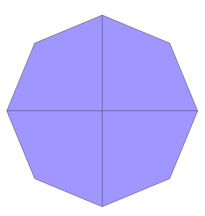
(a) $T_{0}$

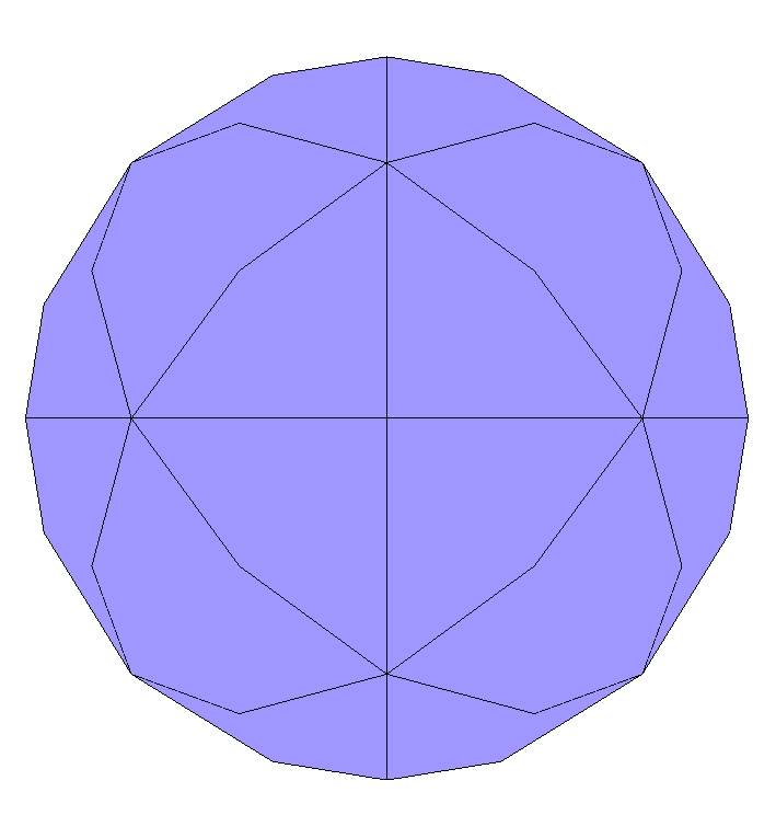
(b) $T_{1}$

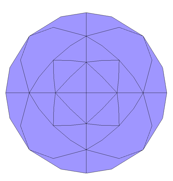
(c) $T_{2}$

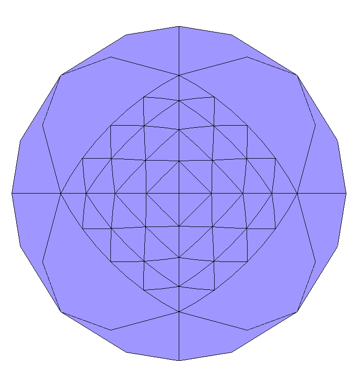
(d) $T_{3}$

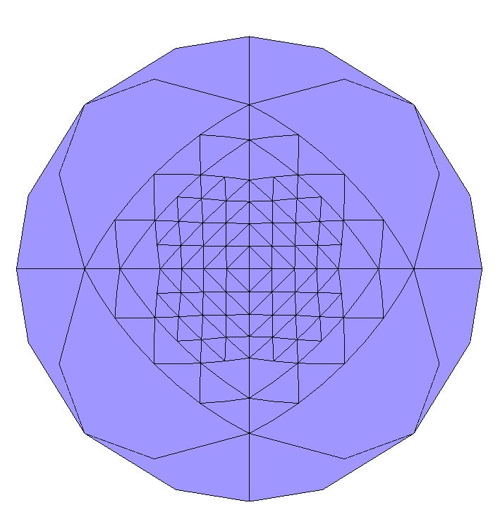
(e) $T_{4}$

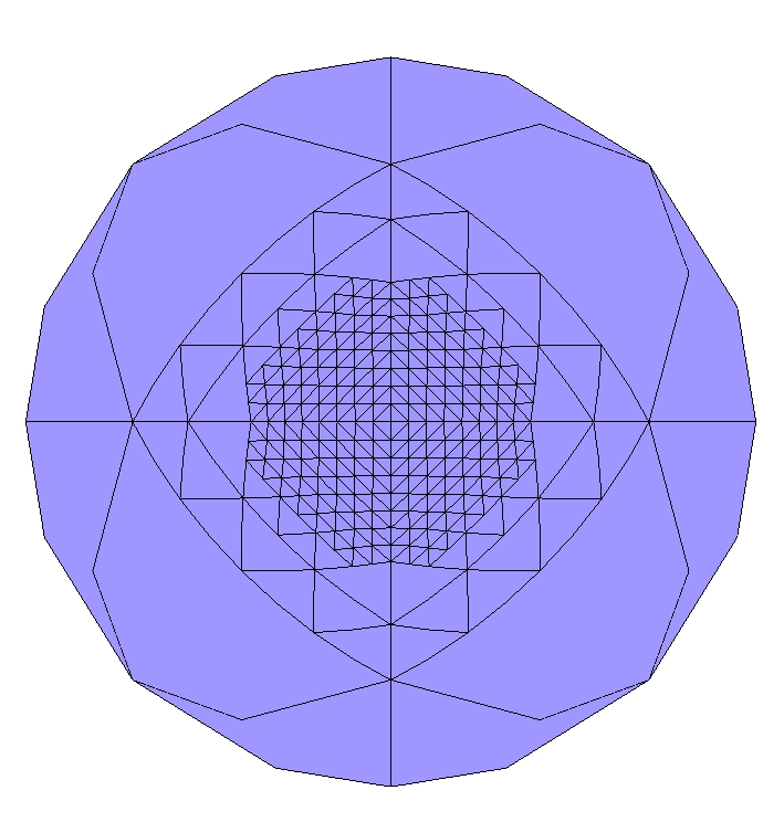
(f) $T_{5}$

Figure 2: A set of nested angular meshes. Mesh $T_{5}$ is the finest mesh. The mesh elements are shown as bisected triangles rather than as spherical triangles. This is due to the plotting.

The prolongation operator follows naturally from the use of a nested discontinuous finite element space, i.e. the complete angular solution can be prolongated without approximation from the coarse to the fine grid by Galerkin projection. The restriction operator is the transpose of prolongation operator, i.e. $R=P^{T}$.

As smoother the standard source iteration procedure is used. Hence we perform iterations of the form

$$L_{l}\phi_{l}^{k+1}=S_{l}\phi_{l}^{k}+f_{l}$$ (17)

where k is the iteration index.

The coarse mesh problems are formulated by direct discretization (Discretization Coarse Grid Approximation, DCA). This procedure is compatible with our matrix-free implementation of the transport solver. Solution on the coarsest level could be performed by source iteration. This is however not effective for highly anisotropic scatter. In Section 5.2 we describe a more effective approach.

5 Results

Although our method is general in terms of scattering functions used we focus on the Fokker-Planck equivalent scatter kernel. For such scatter kernels we have that the Legendre moments are given by

$$\sigma_{s,n}=\frac{\alpha}{2}\left(N(N+1)-n(n+1)\right)$$ (18)

where $\alpha$ is the momentum transfer coefficient. In the present paper we will vary the scatter order, $N$, to increase the forward-peaked nature of the scatter kernel. The normalized scatter cross section for varying $N$ is shown in Figure 3.

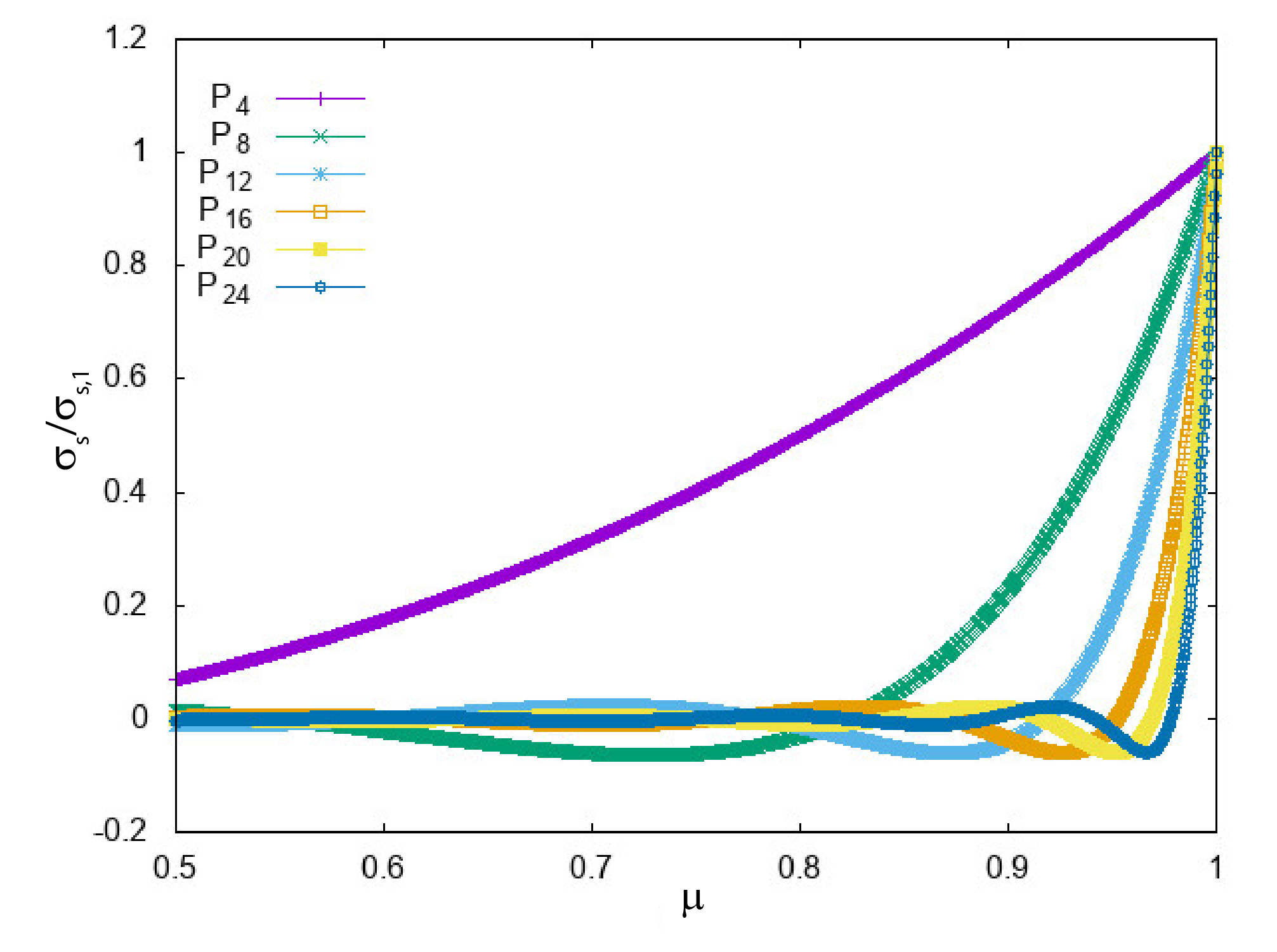
Figure 3: Scatter cross section normalized to maximum value as function of $\mu$ for different expansion orders, $N$.

5.1 Preliminary multigrid performance

In this section we present a preliminary study of multigrid performance and a discussion of the aspects that are crucial for obtaining an efficient method.

We apply the basic multigrid algorithm to a radiation transport problem in a cube of size $5\times 5\times 5\ cm^{3}$. The geometry is meshed with $30\times 30\times 30$ hexahedral elements. The meshes were produced by Gmsh [3]. Boundary conditions are vacuum on all sides and the problem is driven by a uniform isotropic unit strength source in the cube. The transport cross section is equal to 1 and the scatter moments are calculated from equation 18.

We use the multigrid V-cycle with the transport sweep as smoother, inter grid transfers based on Galerkin projection, discussed previously and a thorough coarse grid solution. The stop criterion is chosen as $||r||/||b||<10^{-8}$ where $r$ is the residual vector and $b$ the right hand side. The stop criterion for the coarse grid solver is set to $10^{-5}$. Uniformly refined angular meshes are used. Angular discretization is based on constant and linear basis functions.

For different angular refinement levels on the finest mesh (l = 1, 2, or 3), we investigate the effects of the number of smoothing cycles and restricting the scatter order on the coarse level to $N_{r}<N$ on the multigrid performance. The results for the number of iterations obtained are given in Table 1.

Table 1: Iteration counts for isotropically refined angular meshes (l) up to level 3 and scatter orders N of 4,8 and 16 for the 3D box problem with uniform isotropic source for single grid (SG), different multigrid cycles and limited scatter orders $N_{r}$ on the coarsest level.

basis	l	$N_{r}$	SG	V(1,1)	V(2,1)	SG	V(1,1)	V(2,1)	SG	V(1,1)	V(2,1)
			$N=4$			$N=8$			$N=16$
const	1	0	39	14	14	93	22	22	179	42	42
const	1	1		7	7		12	11		18	16
const	1	2		7	7		11	11		19	19
const	2	0	43	15	14	103	33	33	187	49	42
const	2	1		9	8		17	15		24	23
const	2	2		9	8		17	15		26	23
const	3	0	44	17	15	121	34	34	253	111	210
const	3	1		9	8		19	18		50	34
const	3	2		9	8		20	17		40	36
const	3	3					17	14		32	28
lin	1	0	44	15	14	127	45	33	287	245	231
lin	1	1		6	5		15	14		51	47
lin	1	2		5	4		12	9		26	22
lin	1	3					9	9		22	21
lin	2	0	45	14	14	123	42	32	294
lin	2	1		5	4		14	11		43	41
lin	2	2		4	4		9	8		23	21
lin	2	3					9	8		22	18
lin	3	0	44	13	12	124	31	31	284
lin	3	1		4	4		11	12		31	36
lin	3	2		4	3		8	7		22	22
lin	3	3					4	3		22	20

The main conclusions that can be drawn from this table are as follows: (i) Source iteration is an excellent smoother with V(1,1) not performing significantly worse than V(2,1). Considering the amount of work in smoothing, V(1,1) is favorable in all cases and V(2,1) is not considered throughout the remainder of the paper. (ii) Multigrid performance depends strongly on the choice of scatter order, $N_{r}$, in the coarse grid problem. The iteration counts decrease with increasing $N_{r}$. The iteration counts are consistently much lower than when using the single grid solver and more so for higher scatter anisotropy. Timings are not given in this table as the coarse grid problem has been deliberately solved accurately to investigate optimal multigrid performance and this part dominates the solution time in this approach. It is concluded that in order to build an effective acceleration technique for anisotropic scatter using multigrid, the coarse grid problem needs to be based on a scatter order that is sufficiently high. Using standard source iteration as solver on the coarse angular mesh however requires many steps to reduce the error adequately defying the goal of a cheap solution on the coarse angular mesh. An alternative approach is required for the coarse level.

5.2 Alternative coarse grid solver

The results using the exact solution at the coarsest grid indicate clearly that the coarse grid operator needs to include sufficiently high scatter orders for the multigrid algorithm to be efficient. The use of isotropic or linear anisotropic scatter leads to poor convergence ruling out DSA and its variations. Standard source iteration is a (reasonably) efficient smoother but not a good solution method for anisotropic scattering media, even on the coarsest angular grid.

Our previous work on the Fokker-Planck equation [6] has shown that for that case a good solver is obtained by performing a block Gauss-Seidel iteration over the angular elements, with 10 such sweeps being sufficient on the coarse level. Here, in the Legendre-scatter case we follow the same route: instead of using source iteration, a Gauss-Seidel technique is used. Such a Gauss-Seidel technique is easily implemented by first expanding the source vector given by the usual Legendre summation

$$Q(\textbf{r},\mathbf{\Omega})=\sum_{n,o}\sigma_{s,n}\Phi_{n,o}(\textbf{r})Y_{n,o}(\mathbf{\Omega})$$ (19)

with the flux moments defined as

$$\Phi_{n,o}(\textbf{r})=\int_{4\pi}\phi(\textbf{r},\mathbf{\Omega})Y_{n,o}(\mathbf{\Omega})d\mathbf{\Omega}$$ (20)

Inserting and expanding the flux moments leads to the discrete source, $Q_{[j,q]lm}$

$$Q_{[j,q]lm}=\sum_{p\in P_{j},d,i}N_{[j]li}\sum_{n,o}\sigma_{s,n}X_{[p],d,n,o}X_{[q],m,n,o}\phi\indices{{}_{[j,p]}^{id}}$$ (21)

where

$$X_{[q],m,n,o}=\int_{D_{q}}\Psi_{[q]m}(\mathbf{\Omega})Y_{n,o}(\mathbf{\Omega})d\mathbf{\Omega}$$ (22)

These integrals are pre-calculated and stored. On a given spatial element $j$ and angular element, $q$, a linear system can be solved considering all flux unknowns outside $j$,$q$ as given. The order in which the spatial and angular elements are visited is equal to the order in the standard sweep. This iteration has shown to be effective on the coarse grid. As in our previous work, 10 of such sweeps are sufficient. This coarse grid solver is used throughout the remainder of this work.

5.3 Reduced multigrid scatter order

The algorithm discussed in Section 5.2 - replacing the coarse mesh solver by the alternative sweep solver - is not optimal. Especially the large number of scatter moments involved for large $N$ is detrimental for performance. In the present section we investigate the performance of the multigrid algorithm when operating with reduced scatter order in the multigrid preconditioning stage. We consider the same problem as before, i.e. the box geometry with isotropic uniform source with an angular mesh that is 3 times isotropically refined. The multigrid preconditioner uses a reduced maximum scatter order $N_{r}$. We use 10 sweeps on the coarsest grid. The stop criterion is $||r||/||b||<10^{-8}$. The results of varying $N_{r}$ for different angular basis functions, and different cycles (V(1,0) and V(1,1)), are shown in Figure 4.

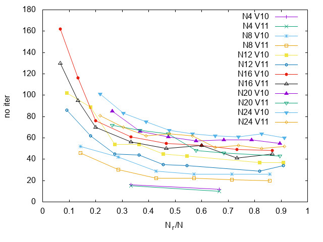
(a) Iteration counts for constant angular basis functions.

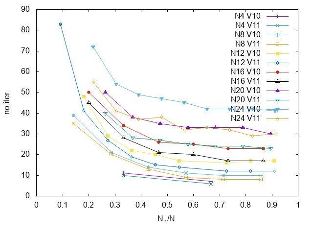
(b) Iteration counts for linear angular basis functions.

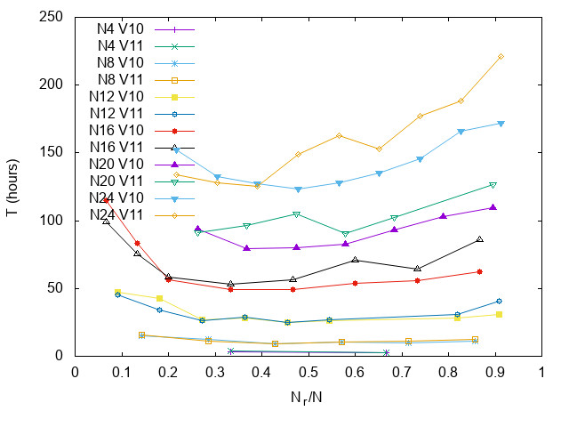
(c) Computational time for constant angular basis functions.

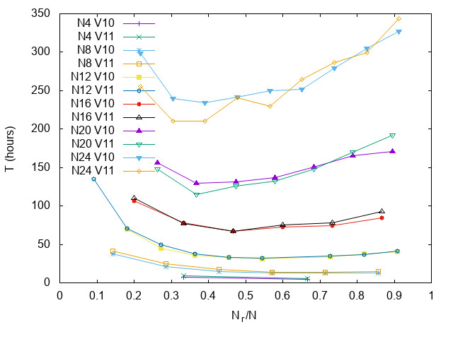
(d) Computational time for linear angular basis functions.

Figure 4: Effectivity of the multigrid algorithm for varying levels of the scatter order for the multigrid preconditioner using the V(1,0) and V(1,1) cycles for the 3D box geometry with uniform source and isotropic angular refinement. Iteration counts given in a and b. Computational times are given in c and d. Constant angular basis functions used in a and c. Linear basis is used in b and d.

The number of iterations required as function of $N_{r}$ decreases with the observation that linear basis function require less iterations than constant basis functions. This may be related to the interpolation operators in the constant basis function case not being accurate enough: Mesh independent multigrid convergence can only be obtained when the following condition is met: $m_{P}+m_{R}>2m$ where $m_{P}$ and $m_{R}$ are the order of polynomial that can be exactly prolongated, and restricted and $2m$ is the order of the differential equation. Although this can be improved by using more complex operators the main target of the paper is the higher-order basis functions, hence this approach has not been pursued.

Concerning the computational time, there is a clear optimum choice of $N_{r}$. On the one hand a small value of $N_{r}$ gives little computational cost but it is not very effective. On the other hand, large values of $N_{r}$ give more optimal multigrid performance but at great expense per iteration. The optimal choice adopted in the remainder of this paper are $N_{r}=2,4,6,7,8,9$ for $N=4,8,12,16,20,24$, respectively. This choice is not very sensitive as long as $N_{r}$ is not chosen on the low side where the computational cost rises quickly with decreasing $N_{r}$.

5.4 Final results on cubic domain

To illustrate the efficiency of the final multigrid procedure using the alternative sweep on the coarsest grid as solver and the reduced scatter order in the multigrid preconditioner we compare the single mesh algorithm to the multigrid algorithm in terms of the number of Krylov iterations and the computational time used. Figure 5 illustrates the main results where the parameters varied are the multigrid cycle used (V(1,0) and V(1,1)) and the scatter order $N$ which is varied between the relatively smooth case of $N=4$ and very forward peaked $N=24$.

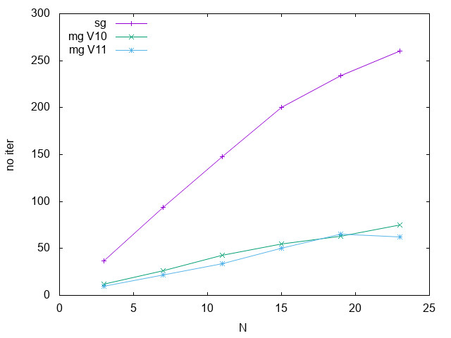
(a) Iteration counts for constant angular basis functions.

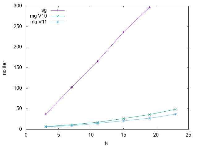
(b) Iteration counts for linear angular basis functions.

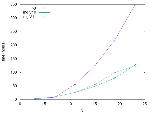
(c) Computational time for constant angular basis functions.

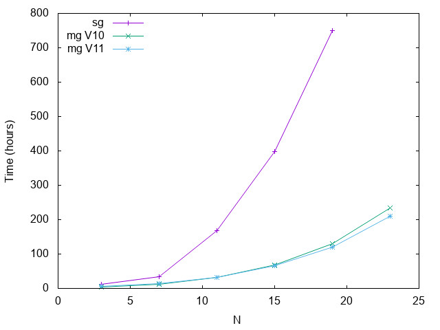
(d) Computational time for linear angular basis functions.

Figure 5: Number of Krylov iterations and computational time for the standard sweep and the multigrid preconditioner using the V(1,0) and V(1,1) cycles for the 3D box geometry with uniform source and isotropic angular refinement. Iteration counts given in a and b. Computational times are given in c and d. Constant angular basis functions used in a and c. Linear basis is used in b and d.

It is clear that the multigrid preconditioner gives a great enhancement of the performance compared to the single grid case both in terms of the number of Krylov iterations required and more importantly in terms of computational effort. As seen before, the constant basis functions do not lead to the same performance enhancements as the linear basis. Both sets of basis functions show the multigrid advantage to increase as the scatter order increases. The computational time saved is between 3 for the constant basis case (at $N=24$) and 6.5 for the linear basis case (at $N=20$, as the single grid at $N=24$ were considered too expensive to run).

5.5 Cubic domain with a boundary source

Following Turcksin and Morel [12] and our previous work on Fokker-Planck solution using multigrid [6] we consider the same cubic domain as earlier but impose a boundary source composed of a pencil beam in the z-direction on part of the cube surface

$$\phi(\textbf{r},\mathbf{\Omega})=\delta(\textbf{r},\mathbf{\Omega}-\textbf{r},\mathbf{\Omega}_{z}),\;z=0,\;2<x,y<3$$ (23)

The Dirac function is used in the DG formalism (see [6]). To capture the forward peaked radiative field due to the boundary condition used, we use a refined angular mesh concentrating elements on the z-pole of the sphere. For a given maximum level $l_{max}$ in the angular, elements with $\Omega_{z}>0.97$ are assigned this refinement level, elements with $0.9<\Omega_{z}<0.97$ are assigned level $l_{max}-1$, elements with $0.8<\Omega_{z}<0.9$ are assigned level $l_{max}-2$, elements with $0.6<\Omega_{z}<0.8$ are assigned level $l_{max}-3$, and all remaining elements are assigned level $l_{max}-4$. The angular meshes contain 20, 32, 44, 128, 440 and 1388 angular elements for $l_{max}$ between 1 and 6. Some of theses meshes are shown in Figure 6. The non-isotropic refinement is one of the advantages of the present method over discrete ordinates techniques for highly non-isotropic radiative fields.

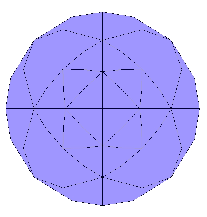
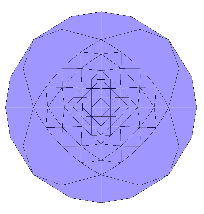
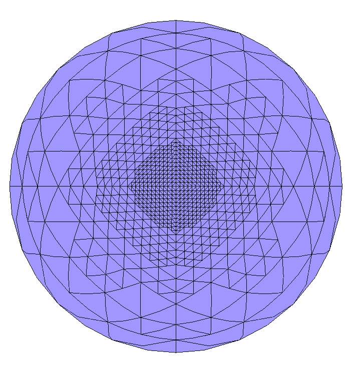
Figure 6: Non-isotropically refined angular meshes corresponding to $l_{max}$ = 2 (left), 4 (middle), 6 (right). The meshes are viewed from the positive $\Omega_{z}$-direction.

The results of the multigrid preconditioned method versus the regular sweep preconditioner are shown in Figure 7.

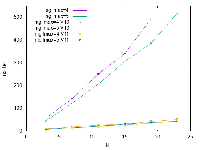
(a) Iteration counts for constant angular basis functions.

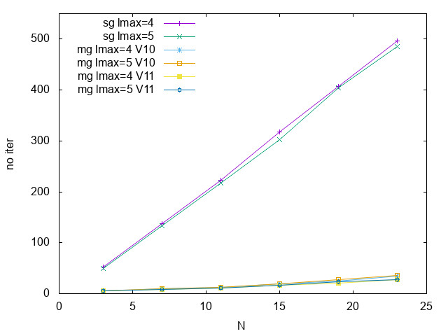
(b) Iteration counts for linear angular basis functions.

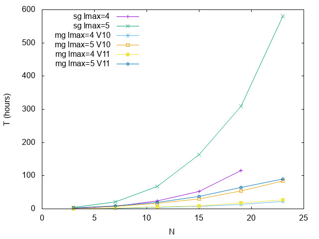
(c) Computational time for constant angular basis functions.

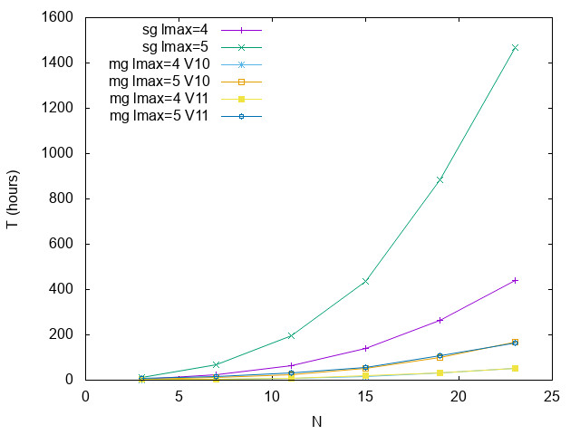
(d) Computational time for linear angular basis functions.

Figure 7: Number of Krylov iterations and computational time for the standard sweep and the multigrid preconditioner using the V(1,0) and V(1,1) cycles for the 3D box geometry with boundary source and anisotropic angular refinement with varying depth $l_{max}$. Iteration counts given in a and b. Computational times are given in c and d. Constant angular basis functions used in a and c. Linear basis is used in b and d.

As in the isotropically refined case, the multigrid based solver gets increasingly efficient w.r.t. to the single grid case with higher scatter order $N$. Here, the savings are even greater, i.e. up to around a factor of 6 for the constant basis functions ($N=24$) and up to a factor of around 9 for the linear basis ($N=24$). Finally, the effect of choice of multigrid cycling strategy is of little influence for the efficiency.

6 Conclusions

The standard transport sweep is not an effective preconditioner for the transport equation in the presence of highly forward scatter. Diffusion synthetic acceleration is also known not to be effective in these cases. In this work we have adapted an angular multigrid preconditioner originally developed for the Fokker-Planck equation to the case using Legendre scatter modeling. Interpolation operators are defined naturally through the hierarchic nature of the discontinuous Galerkin angular discretization. Smoothing on each level is effected by the standard source iteration technique. A new sweep algorithm was developed that is better capable of solving the coarse mesh problem, even for high scatter orders.

The multigrid preconditioner was used in several test cases. The first test case consists of a 3D geometry with a uniform isotropic source. Uniform angular refinement is used. It was found that the most effective strategy is to use a reduced scatter order for the multigrid preconditioner. The optimal value was found to increase slightly with the scatter order, $N$. Using this optimal value, a comparison was done with the standard sweep preconditioner in terms of number of Krylov iterations required and the computational time to solve the problem. In all cases the multigrid preconditioner outperformed the sweep algorithm, especially for the linear angular basis. With increasing scatter order, the difference between sweep and multigrid become greater. Another test case is a 3D geometry with a uni-directional boundary source. Here, the angular meshes are anisotropically refined to capture the anisotropic radiation field induced by the boundary condition. The multigrid preconditioner was again highly effective compared to the sweep preconditioner with similar trends as found in the volumetric source case.

References

- de Oliveira et al. [2000] C.R.E. de Oliveira, C.C. Pain, and M. Eaton. Hierarchical Angular Preconditioning for the Finite Element Spherical Harmonics Radiation Transport Method. In Proceedings of PHYSOR 2000, International Topical Meeting on Advances in Reactor Physics and Mathematics and Computation into the Next Millenium. Americal Nuclear Society, 2000.
- Drumm and Fan [2017] C.R. Drumm and W.C. Fan. Multilevel Acceleration of Scattering-source Iterations with Application to Electron Transport. Nuclear Engineering and Technology, 49:1114–1124, 2017.
- Geuzaine and Remacle [2009] C. Geuzaine and J.F. Remacle. Gmsh: A Three-dimensional Finite Element Mesh Gemerator with Built-in Pre- and Post-processing Facilities. Int. Journal for Numerical Methods in Engineering, 79(11):1309–1331, 2009.
- Hennink and Lathouwers [2017] A. Hennink and D. Lathouwers. A Discontinuous Galerkin Method for the Mono-Energetic Fokker-Planck Equation based on a Spherical Interior Penalty Formulation. Journal of Computational and Applied Mathematics, 330:253–267, 2017.
- Kópházi and Lathouwers [2015] J. Kópházi and D. Lathouwers. A Space-Angle DGFEM Approach for the Boltzmann Radiation Transport Equation with Local Angular Refinement. Journal of Computational Physics, 297:637–668, 2015.
- Lathouwers and Perkó [2019] D. Lathouwers and Z. Perkó. An Angular Multigrid Preconditioner for the Radiation Transport Equation with Fokker-Planck Scattering. Journal of Computational and Applied Mathematics, 350:165–177, 2019.
- Lee [2010a] B. Lee. A Novel Multigrid Method for SN Discretizations of the Mono-Energetic Boltzmann Transport Equation in the Optically Thick and Thin Regimes with Anisotropic Scatter, Part I. SIAM J. Sci. Comput., 31(6):4744–4773, 2010a.
- Lee [2010b] B. Lee. Improved Multiple-Coarsening Methods for SN Discretizations of the Bolltzmann Equation. SIAM J. Sci. Comput., 32(5):2497–2522, 2010b.
- Morel and Manteuffel [1999] J.E. Morel and T.A. Manteuffel. Two-Level Fourier Analysis of a Multigrid Approach for Discontinuous Galerkin Discretizations. Nucl. Sci. and Engng., 107:330–342, 1999.
- Pain et al. [2006] C.C. Pain, M.D. Eaton, R.P. Smedley-Stevenson, A.J.H. Goddard, M.D. Piggott, and C.R.E. de Oliveira. Space-Time Streamline Upwind Petrov-Galerkin Methods for the Boltzmann Transport Equation. Comput. Methods Appl. Mech. Engrg., 195:4334–4357, 2006.
- Pautz et al. [1999] S. Pautz, J.E. Morel, and M.L. Adams. An Angular Multigrid Aceleration Method for the SN Equations with Highly Forward-Peaked Scattering. In Proceedings of International Conference on Mathematics and Computation, Reactor Physics and Environmental Analyses in Nuclear Applications. Americal Nuclear Society, 1999.
- Turcksin et al. [2012] B. Turcksin, J.C. Ragusa, and J.E. Morel. Angular Multigrid Preconditioner for Krylov-Based Solution Techniques Applied to the Sn Equations with Highly Forward-Peaked Scattering. Transport Theory and Statistical Physics, 41(1-2):1–22, 2012.
- Van der Vorst [1992] H.A. Van der Vorst. Bi-CGSTAB: A Fast and Smoothly Converging Variant of Bi-CG for the Solution of Nonsymmetric Linear Systems. SIAM J. Sci. and Stat. Comput., 13(2):631–644, 1992.
- Wesseling [1992] P. Wesseling. An Introduction to Multigrid Methods. John Wiley and Sons, 1992.