Uniform deconvolution for Poisson Point Processes

Abstract

We focus on the estimation of the intensity of a Poisson process in the presence of a uniform noise. We propose a kernel-based procedure fully calibrated in theory and practice. We show that our adaptive estimator is optimal from the oracle and minimax points of view, and provide new lower bounds when the intensity belongs to a Sobolev ball. By developing the Goldenshluger-Lepski methodology in the case of deconvolution for Poisson processes, we propose an optimal data-driven selection of the kernel bandwidth. Our method is illustrated on the spatial distribution of replication origins and sequence motifs along the human genome.

Keywords: Convolution, Poisson Point Process, Adaptive estimation

1 Introduction

Inverse problems for Poisson point processes have focused much attention in the statistical literature over the last years, mainly because the estimation of a Poisson process intensity in the presence of additive noise is encountered in many practical situations like tomography, microscopy, high energy physics. Our work is motivated by an original application field in high throughput biology, that has been revolutionized by the development of high throughput sequencing. The applications of such technologies are many, and we focus on the particular cases where sequencing allows the fine mapping of genomic features along the genome, like transcription factors. The spatial distribution of these features can be modeled by a Poisson process with unknown intensity. Unfortunately, detections are prone to some errors, which produces data in the form of genomic intervals whose width is linked to the precision of detection. Since the exact position of the peak is unknown within the interval (and not necessarily positioned at the center on average), the appropriate error distribution is uniform, the level of noise being given by the width of the intervals. Another example is provided when studying the spatial distribution of sequence motifs along the genome. A sequence motif is a pattern of nucleotides that is widespread along the genome, with potentially unknown function, but whose frequent occurrence suggests some implication in biological pathways. G-quadruplexes motifs for instance are made of guanine (G) repeats in tetrads that form particular 3D structures whose biologically function is currently unknown (Chambers et al., 2015). However their implication in replication initiation has now been demonstrated (Picard et al., 2014) among other biological functions. These motifs are $\sim 25-30$ nucleotide long, and when studying their spatial distribution, their occurrence can be modelled by a Poisson process, and the uniform error model recalls that the data are in the form of intervals, without any reference occurrence point within the interval. Hence the spatial distribution of these motifs should be deconvoluted from this uniform error.

In the 2000s, several wavelet methods have been proposed for Poisson intensity estimation from indirect data (Antoniadis and Bigot, 2006), as well as B-splines and empirical Bayes estimation (Kuusela et al., 2015). Other authors turned to variational regularization: see the survey of Hohage and Werner (2016), which also contains examples of applications and reconstruction algorithms. From a more theoretical perspective, Kroll (2019) studied the estimation of the intensity function of a Poisson process from noisy observations in a circular model. His estimator is based on Fourier series and is not appropriate for uniform noise (whose Fourier coefficients are zero except the first).

The specificity of uniform noise has rather been studied in the context of density deconvolution. In this case also, classical methods based on the Fourier transform do not work either in the case of a noise with vanishing characteristic function (Meister, 2009). Nevertheless several corrected Fourier approaches were introduced (Hall et al., 2001, 2007; Meister, 2008; Feuerverger et al., 2008). In this line, the work of Delaigle and Meister (2011) is particularly interesting, even if it is limited to a density to estimate with finite left endpoint. In a recent work, Belomestny and Goldenshluger (2021) have shown that the Laplace transform can perform deconvolution for general measurement errors. Another approach consists in using Tikhonov regularization for the convolution operator (Carrasco and Florens, 2011; Trong et al., 2014). In the specific case of uniform noise (also called boxcar deconvolution), it is possible to use ad hoc kernel methods (Groeneboom and Jongbloed, 2003; van Es, 2011). In this context of non-parametric estimation, each method depends on a regularization parameter (such as a resolution level, a regularization parameter or a bandwidth), and only a good choice of this parameter allows to achieve an optimal reconstruction. This parameter selection is often named adaptation since the point is to adapt the parameter to the features of the target density. The above cited works (except Delaigle and Meister (2011)) do not address this adaptation issue or only from a practical point of view, although this is central both from the practical and theoretical points of views.

We propose a kernel estimator to estimate the intensity of a Poisson process in the presence of a uniform noise. We provide theoretical guarantees of its performance by deriving the minimax rates of convergence of the integrated squared risk for an intensity belonging to a Sobolev ball. To ensure the optimality of our procedure, we establish new lower bounds on this smoothness space. Then we provide an adaptive procedure for bandwidth selection using the Goldenshluger-Lepski methodology, and we show its optimality in the oracle and minimax frameworks. From the practical point of view we tune the method based on simulations to determine a consensus value for the hyperparameter. The empirical performance of our estimator is then studied by simulations and competed with a deconvolution method based on Gaussian errors. Finally we provide an illustration of our procedure on experimental data in Genomics, where the purpose is to study the spatial repartition of replication starting points and sequence motifs along chromosomes in humans (Picard et al., 2014). The code is available at https://github.com/AnnaBonnet/PoissonDeconvolution.

2 Uniform deconvolution model

We consider $(X_{i})_{i}$, the realization of a Poisson Process on $\mathbb{R}$, denoted by $N^{X}$, with $N_{+}:=N^{X}(\mathbb{R})$ the number of occurrences. The uniform convolution model consists in observing $(Y_{i})_{i}$, occurrences of a Poisson process $N^{Y}$, a noisy version of $N^{X}$ corrupted by a uniform noise, such that:

$$\forall\,i\in\{1,\ldots,N_{+}\},\quad Y_{i}=X_{i}+\varepsilon_{i},\quad\varepsilon_{i}\sim\mathcal{U}[-a;a],$$ (2.1)

where $a$, assumed to be known, is fixed. The errors $(\varepsilon_{i})_{i}$ are supposed mutually independent, and independent of $(X_{i})_{i}$. Then, we denote by $\lambda_{X}$ the intensity function of $N^{X}$, and $\mu_{X}$ its mean measure assumed to satisfy $\mu_{X}(\mathbb{R})<\infty$, so that

$$d\mu_{X}(x)=\lambda_{X}(x)dx,\quad x\in\mathbb{R}.$$

Note that $N_{+}\sim{\mathcal{P}}(\mu_{X}(\mathbb{R})),$ where ${\mathcal{P}}(\theta)$ denotes the Poisson distribution with parameter $\theta$. Then we further consider that observing $N^{X}$ with intensity $\lambda_{X}$ is equivalent to observing $n$ i.i.d. Poisson processes with common intensity $f_{X}$, with $\lambda_{X}=n\times f_{X}$. This specification will be convenient to adopt an asymptotic perspective. As for $\lambda_{Y}$, the intensity of $N^{Y}$, it can easily be shown that

$$n^{-1}\times\lambda_{Y}=n^{-1}\times(\lambda_{X}\star f_{\varepsilon})=f_{X}\star f_{\varepsilon}=:f_{Y},$$

where $f_{\varepsilon}$ stands for the density of the uniform distribution. The goal of the deconvolution method is to estimate $f_{X}$, based on the observation of $N^{Y}$ on a compact interval $[0,T]$ for some fixed positive real number $T$. In the following, we provide an optimal estimator of $f_{X}$ in the oracle and minimax settings. Minimax rates of convergence will be studied in the asymptotic perspective $n\to+\infty$ and parameters $a$ and $T$ will be viewed as constants. Furthermore, $\|f_{X}\|_{1}$, the $\mathbb{L}_{1}$-norm will be assumed to be larger than an absolute constant, denoted by $r$.

Notations.

We denote by $\|\cdot\|_{2,T}$, $\|\cdot\|_{1,T}$ and $\|\cdot\|_{\infty,T}$ the $\mathbb{L}_{2}$, $\mathbb{L}_{1}$ and sup-norm on $[0;T]$, and $\|\cdot\|_{2}$, $\|\cdot\|_{1}$, and $\|\cdot\|_{\infty}$ their analog on $\mathbb{R}$. Notation $\lesssim$ means that the inequality is satisfied up to a constant and $a_{n}=o(b_{n})$ means that the ratio $a_{n}/b_{n}$ goes to 0 when $n$ goes to $+\infty$. Finally, $\llbracket a;b\rrbracket$ denotes the set of integers larger or equal to $a$ and smaller or equal to $b$.

3 Estimation procedure

3.1 Deconvolution with kernel estimator

To estimate $f_{X}$ based on observations of $N^{Y}$, we introduce a kernel estimator which is based on the following heuristic arguments inspired from van Es (2011) who considered the setting of uniform deconvolution for density estimation. We observe that $f_{Y}$ can be expressed by using the cumulative distribution of the $X_{i}$’s:

$$F_{X}(x):=\int_{-\infty}^{x}f_{X}(u)du\leq\|f_{X}\|_{1},\quad x\in\mathbb{R}.$$

Indeed, for $x\in\mathbb{R}$,

$$f_{Y}(x) =\int_{\mathbb{R}}f_{X}(x-u)f_{\varepsilon}(u)du$$

$$=\frac{1}{2a}\int_{-a}^{a}f_{X}(x-u)du$$

$$=\frac{1}{2a}\bigg{(}F_{X}(x+a)-F_{X}(x-a)\bigg{)},$$ (3.1)

from which we deduce:

$$F_{X}(x)=2a\sum_{k=0}^{+\infty}f_{Y}\bigg{(}x-(2k+1)a\bigg{)},\quad x\in\mathbb{R}.$$

Then, from heuristic arguments, we get

$$f_{X}(x)=2a\sum_{k=0}^{+\infty}f^{\prime}_{Y}\bigg{(}x-(2k+1)a\bigg{)},$$ (3.2)

which provides a natural form of our kernel estimate $\widehat{f}_{Y}$. Note that differentiability of $f_{Y}$ is not assumed in the following. Indeed, we consider the kernel estimator of $f_{Y}$ such that

$$\widehat{f}_{Y}(x)=\frac{1}{nh}\int_{\mathbb{R}}K\left(\frac{x-u}{h}\right)dN^{Y}_{u},$$

with $dN^{Y}$ the point measure associated to $N^{Y}$, and $K$ a kernel with bandwidth $h>0$. Setting

$$K_{h}(x)=\frac{1}{h}K\bigg{(}\frac{x}{h}\bigg{)},$$

we can write

$$\widehat{f}_{Y}(x)=\frac{1}{n}\sum_{i=1}^{N_{+}}K_{h}\big{(}x-Y_{i}\big{)}.$$

Then, if $K$ is differentiable, we propose the following kernel-based estimator of $f_{X}$

$$\widehat{f}_{h}(x)=\frac{2a}{nh^{2}}\sum_{k=0}^{+\infty}\sum_{i=1}^{N_{+}}K^{\prime}\left(\frac{x-(2k+1)a-Y_{i}}{h}\right).$$

The proof of subsequent Lemma 1 in Appendix shows that the expectation of $\widehat{f}_{h}$ is a regularization of $f_{X}$, as typically desired for kernel estimates since we have

$$\mathbb{E}[\widehat{f}_{h}]=K_{h}\star f_{X}.$$ (3.3)

Then, our objective is to provide an optimal selection procedure for the parameter $h$.

3.2 Symmetrization of the estimator

Our estimator is based on the inversion and differentiation of Equation (3.1), which can also be performed as follows:

$$2a\sum_{k=0}^{+\infty}f_{Y}(x+(2k+1)a)=\sum_{k=0}^{+\infty}\bigg{(}F_{X}(x+2(k+1)a)-F_{X}(x+2ka)\bigg{)}=\|f_{X}\|_{1}-F_{X}(x)$$

and differentiated to obtain:

$$f_{X}(x)=-2a\sum_{k=0}^{+\infty}f^{\prime}_{Y}\bigg{(}x+(2k+1)a\bigg{)},$$

which leads to another estimator

$$\check{f}_{h}(x)=-\frac{2a}{nh^{2}}\sum_{k=0}^{+\infty}\sum_{i=1}^{N_{+}}K^{\prime}\left(\frac{x+(2k+1)a-Y_{i}}{h}\right).$$

In the framework of uniform deconvolution for densities, van Es (2011) proposes to use $\alpha\hat{f}_{h}(x)+(1-\alpha)\check{f}_{h}(x)$, a convex combination of $\hat{f}_{h}$ and $\check{f}_{h}$, as a combined estimator, to benefit from the small variance of $\check{f}_{h}(x)$ and $\hat{f}_{h}(x)$ for large and small values of $x$ respectively. Unfortunately the combination that minimizes the asymptotic variance of the combined estimator is achieved for $\alpha=1-F_{X}(x)$, and thus depends on an unknown quantity. van Es (2011) suggested to use a plug-in estimator, but to avoid supplementary technicalities, we finally consider the following symmetric kernel-based estimator:

$$\widetilde{f}_{h}(x):=\frac{1}{2}\bigg{(}\hat{f}_{h}(x)+\check{f}_{h}(x)\bigg{)}=\frac{a}{nh^{2}}\sum_{k=-\infty}^{+\infty}s_{k}\sum_{i=1}^{N_{+}}K^{\prime}\left(\frac{x-(2k+1)a-Y_{i}}{h}\right),$$ (3.4)

with $s_{k}=1$ if $k\geq 0$ and $s_{k}=-1$ if $k<0$. Then it is shown in Lemma 1 that

$$\mathbb{E}[\widetilde{f}_{h}]=(K_{h}\star f_{X}).$$

3.3 Risk of the kernel-based estimator

Our objective is to provide a selection procedure to select a bandwidth $\widehat{h}$, that only depends on the data, so that the $\mathbb{L}_{2}$-risk of $\widetilde{f}_{\widehat{h}}$ is smaller than the risk of the best kernel estimate (up to a constant), namely

$$\mathbb{E}\left[\|\widetilde{f}_{\widehat{h}}-f_{X}\|_{2,T}^{2}\right]\lesssim\inf_{h\in{\mathcal{H}}}\mathbb{E}\left[\|\widetilde{f}_{h}-f_{X}\|_{2,T}^{2}\right].$$

Our procedure is based on the bias-variance trade-off of the risk of any estimate $\widetilde{f}_{h}$

$$\mathbb{E}\Big{[}\|\widetilde{f}_{h}-f_{X}]\|_{2,T}^{2}\Big{]} =\|\mathbb{E}[\widetilde{f}_{h}]-f_{X}\|_{2,T}^{2}+\mathbb{E}\Big{[}\|\widetilde{f}_{h}-\mathbb{E}[\widetilde{f}_{h}]\|_{2,T}^{2}\Big{]}$$

$$=:B_{h}^{2}+v_{h}.$$ (3.5)

Then we use the following mild assumption:

Assumption 1

The kernel $K$ is supported on the compact interval $[-A,A]$, with $A\in\mathbb{R}_{+}^{*}$ and $K$ is differentiable on $[-A,A]$.

Then the variance of the estimator is such that:

Lemma 1

For any $h\in\mathcal{H}$ and any $x\in[0,T]$, we have

$$\mathbb{E}[\widetilde{f}_{h}(x)]=(K_{h}\star f_{X})(x).$$

Under Assumption 1 and if $h$ is small enough so that $Ah\leq a$, then

$$v_{h}:=\mathbb{E}\Big{[}\|\widetilde{f}_{h}-\mathbb{E}[\widetilde{f}_{h}]\|_{2,T}^{2}\Big{]}=\frac{aT\|f_{X}\|_{1}\|K^{\prime}\|_{2}^{2}}{2nh^{3}}.$$

The expectation of $\widetilde{f}_{h}$ has the expected expression (derived from (3.3)), but Lemma 1 also provides the exact expression of the variance term $v_{h}$ of our very specific estimate. Since our framework is an inverse problem, this variance does not reach the classical $(nh)^{-1}$ bound. Moreover, $v_{h}$ depends linearly on $\|f_{X}\|_{1}$ but also on $T$, which means that the estimation of $f_{X}$ has to be performed on the compact interval $[0,T]$, for $v_{h}$ to be finite. This requirement is due to Expression (3.4) of our estimate that shows that for any $x\in\mathbb{R}$, $\widetilde{f}_{h}(x)$ is different from 0 almost surely. This dependence of $v_{h}$ on $T$ is a direct consequence of our strategy not to make any assumption on the support of $f_{X}$, that can be unknown or non-compact. Of course, if the support of $f_{X}$ was known to be compact, like $[0,1]$, then we would force $\widetilde{f}_{h}$ to be null outside $[0,1]$ (for instance by removing large values of $|k|$ in the sum of (3.4)), and estimation would be performed on the set $[0,1]$. Actually, estimating a non-compactly supported Poisson intensity on the whole real line leads to deterioration of classical non-parametric rates in general (Reynaud-Bouret and Rivoirard, 2010).

3.4 Bandwidth selection

The objective of our procedure is to choose the bandwidth $h$, based on the Goldenshluger-Lepski methodology (Goldenshluger and Lepski, 2013). First, we introduce a finite set $\mathcal{H}$ of bandwidths such that for any $h\in\mathcal{H}$, $h\leq a/A,$ which is in line with assumptions of Lemma 1. Then, for two bandwidths $t$ and $h$, we also define

$$\widetilde{f}_{h,t}:=K_{h}\star\widetilde{f}_{t},$$

a twice regularized estimator, that satisfies the following property (see Lemma 7 in Appendix):

$$\widetilde{f}_{h,t}=\widetilde{f}_{t,h}.$$

Now we select the bandwidth as follows:

$$\widehat{h}:=\operatorname*{argmin}_{h\in\mathcal{H}}\left\{{\mathcal{A}}(h)+\frac{c\sqrt{N_{+}}}{nh^{3/2}}\right\},$$ (3.6)

where

$$c=(1+\eta)(1+\|K\|_{1})\|K^{\prime}\|_{2}\sqrt{\frac{aT}{2}}$$ (3.7)

for some $\eta>-1$ and

$${\mathcal{A}}(h):=\max_{t\in\mathcal{H}}\left\{\|\widetilde{f}_{h,t}-\widetilde{f}_{t}\|_{2,T}-\frac{c\sqrt{N_{+}}}{nt^{3/2}}\right\}_{+}.$$

Finally, we estimate $f_{X}$ with

$$\widetilde{f}=\widetilde{f}_{\widehat{h}}.$$ (3.8)

Note that ${\mathcal{A}}(h)$ is an estimation of the bias term $B_{h}$ of the estimator $\widetilde{f}_{h}$. Indeed,

$$B_{h}:=\|\mathbb{E}[\widetilde{f}_{h}]-f_{X}\|_{2,T}=\|K_{h}\star f_{X}-f_{X}\|_{2,T}$$

and we replace the unknown function $f_{X}$ with the kernel estimate $\widetilde{f}_{t}$. The term $\frac{c\sqrt{N_{+}}}{nt^{3/2}}$ in ${\mathcal{A}}(h)$ controls the fluctuations of $\|\widetilde{f}_{h,t}-\widetilde{f}_{t}\|_{2,T}$. Finally, since $\mathbb{E}[N_{+}]=n\|f_{X}\|_{1}$, (3.6) mimics the bias-variance trade-off (3.3) (up to the squares). In order to fully define the estimation procedure, it remains to choose the set of bandwidths ${\mathcal{H}}$. This is specified in Section 4.

4 Theoretical results

4.1 Oracle approach

The oracle setting allows us to prove that the bandwidth selection procedure described in Section 3.4 is (nearly) optimal among all kernel estimates. Indeed, we obtain the following result.

Theorem 2

Suppose that Assumption 1 is verified. We take $\eta>0$ and we consider the estimate $\widetilde{f}$ such that the finite set of bandwidths $\mathcal{H}$ satisfies

$$\min\mathcal{H}=1/(\delta n^{\frac{1}{3}})\quad\mbox{and}\quad\max\mathcal{H}=o(1)$$

for some constant $\delta>0$. Then, for $n$ large enough,

$$\mathbb{E}\left[\|\widetilde{f}_{\widehat{h}}-f_{X}\|_{2,T}^{2}\right]\leq C_{1}\inf_{h\in{\mathcal{H}}}\mathbb{E}\left[\|\widetilde{f}_{h}-f_{X}\|_{2,T}^{2}\right]+\frac{C_{2}}{n},$$ (4.1)

where $C_{1}=2+24(1+\eta)^{2}(1+\|K\|_{1})^{2}$ and $C_{2}$ is a constant depending on $\|f_{X}\|_{1}$, $T$, $a$, $\delta,$ $\eta$ and $K$.

The proof of this result can be found in Section 7.3, where the expression of $C_{2}$ is provided (see Equation (7.3)).

Remark 3

Note that condition $h\geq\delta^{-1}n^{-1/3}$ is equivalent to $\sup_{n}\sup_{h\in{\mathcal{H}}}v_{h}<\infty$

Remark 4

Equation (7.3) provides the explicit dependence of $C_{2}$ on $a,$ $\delta,$ $\eta,$ $T$ and $K$, showing that the kernel $K$ has to be chosen such that $\|K\|_{1},$ $\|K^{\prime}\|_{\infty}$, $\|K\|_{2},$ $\|K^{\prime}\|_{1}$ and $\|K^{\prime}\|_{2}$ are as small as possible. Nevertheless, in the minimax approach of Section 4.2, the kernel has to satisfy some constraints (see Assumption 2). The parameter $a$ is present in the remainder term of the risk bound in the following way $C_{2}/n=(k_{0}+k_{1}a+k_{2}a^{2})/n$. Thus the larger $a$ the worse the bound, this is expected since $a$ measures the noise level.

Theorem 2 shows that our procedure achieves nice performance: Up to the constant $C_{1}$ and the negligible term $C_{2}/n$ that goes to 0 quickly, our estimate has the smallest risk among all kernel rules under mild conditions on the set of bandwidths $\mathcal{H}.$

4.2 Minimax approach

The minimax approach is a framework that shows the optimality of an estimate among all possible estimates. For this purpose, we consider a class of functional spaces for $f_{X}$, then we derive the minimax risk associated with each functional space and show that our estimator achieves this rate. Here, we consider the class of Sobolev balls that can be defined, for instance, through the Fourier transform of $\mathbb{L}_{2}$-functions: Given $\beta>0$, $L>0$, $b>0$ and $r>0$, consider the following subset of the Sobolev ball of smoothness $\beta$ and radius $L$

$${\mathcal{S}}^{\beta}(L,r,b):=\left\{g\in\mathbb{L}_{2}:\quad\int_{-\infty}^{+\infty}|g^{*}(\xi)|^{2}(\xi^{2}+1)^{\beta}d\xi\leq L^{2},\ r\leq\|g\|_{1}\leq bL\right\},$$

where $g^{*}(\xi):=\int e^{ix\xi}g(x)dx$ is the Fourier transform of $g$. Observe that the classical Sobolev space corresponds to the case $r=0$ and $b=+\infty$; $r$ and $b$ will be viewed as constants in the sequel. In the Poisson setting, the ${\mathbb{L}}_{1}$-norm of the Poisson intensity is not fixed but it of course plays a key role in rates. Given $L$, the radius of the Sobolev ball containing $g$, the ${\mathbb{L}}_{1}$-norm of $g$ scales in $L$. We finally introduce the lower bound $\|g\|_{1}\geq r$ with $r>0$ to avoid the asymptotic setting where the Poisson intensity goes to 0.

From a statistical perspective, the minimax rate associated with the space ${\mathcal{S}}^{\beta}(L,r,b)$ is

$${\mathcal{R}}_{n}(\beta,L):=\inf_{Z_{n}}\sup_{f_{X}\in{\mathcal{S}}^{\beta}(L,r,b)}\mathbb{E}\left[\|Z_{n}-f_{X}\|_{2,T}^{2}\right],$$

where the infimum is taken over all estimators $Z_{n}$ of $f_{X}$ based on the observations $(Y_{i})_{i=1,\ldots,N_{+}}.$ In the notation, we drop the dependence of the risk on $r$ and $b$ since we are only interested in the dependence on $n$, $\beta$ and $L$. We first derive a lower bound for the minimax risk.

Theorem 5

We assume that $rL^{-1}\leq\pi/(2\mathfrak{c}_{\beta})\leq b$, where $\mathfrak{c}_{\beta}$ is defined in (7.4). There exists a positive constant $C_{3}$ only depending on $\beta,$ $a$ and $T$ such that, if $n$ is larger than some $n_{0}$ only depending on $r$ and $T$,

$${\mathcal{R}}_{n}(\beta,L)\geq C_{3}\left[L^{\frac{2\beta+6}{2\beta+3}}n^{-\frac{2\beta}{2\beta+3}}+Ln^{-1}\right].$$ (4.2)

Theorem 5 is proved in Section 7.4. To the best of our knowledge, because of the second term $Ln^{-1}$, the rate established in (4.2) is new. Of course, if $L$ is bounded then the second term is negligible with respect to the first one when $n\to+\infty$. The rate $n^{-\frac{2\beta}{2\beta+3}}$ is slower than the classical non-parametric rate $n^{-\frac{2\beta}{2\beta+1}}.$ It is the expected rate since our deconvolution problem corresponds to an inverse problem of order 1, meaning that $f_{\varepsilon}^{*}$, the characteristic function of the noise, satisfies

$$|f_{\varepsilon}^{*}(\xi)|=O(\xi^{-1})\text{ as }\xi\to\infty.$$

Note that the analog of the previous lower bound has been established in the density deconvolution context, first by Fan (1993), but with supplementary assumption $|{f_{\varepsilon}^{*}}^{\prime}(\xi)|=O(\xi^{-2})$ which is not satisfied in our case of uniform noise (see Equation (7.8)). Our proof is rather inspired by the work of Meister (2009), but we face here a Poisson inverse problem, and we have to control the ${\mathbb{L}}_{2}$-norm on $[0,T]$ instead of $\mathbb{R}.$ Furthermore, Theorem 2.14 of Meister (2009) only holds for $\beta>1/2$. Consequently, we use different techniques to establish Theorem 5, which are based on wavelet decompositions of the signal. Specifically, we use the Meyer wavelets of order 2.

We now show that the rate achieved by our estimate $\widetilde{f}$ corresponds to the lower bound (4.2), up to a constant. We have the following corollary, easily derived from Theorem 2, and based on the following assumption.

Assumption 2

The kernel $K$ is of order $\ell=\lfloor\beta\rfloor$, meaning that the functions $x\mapsto x^{j}K(x)$, $j=0,1,\ldots,\ell$ are integrable and satisfy

$$\int K(x)dx=1,\quad\int x^{j}K(x)dx=0,\quad j=1,\ldots,\ell.$$

Remark 6

See Proposition 1.3 of Tsybakov (2008) or Section 3.2 of Goldenshluger and Lepski (2014) for the construction of kernels satisfying Assumptions 1 and 2.

Corollary 1

Suppose that Assumptions 1 and 2 are satisfied. We take $\eta>0$ and we consider the estimate $\widetilde{f}$ such that the set of bandwidths $\mathcal{H}$ is

$$\mathcal{H}=\left\{D^{-1}:\quad D\in\llbracket\log n;\delta n^{\frac{1}{3}}\rrbracket\right\},$$

for some constant $\delta>0$. Then, for $n$ large enough,

$$\sup_{f_{X}\in{\mathcal{S}}^{\beta}(L,r,b)}\mathbb{E}\left[\|\widetilde{f}-f_{X}\|_{2,T}^{2}\right]\leq C_{4}\left[L^{\frac{2\beta+6}{2\beta+3}}n^{-\frac{2\beta}{2\beta+3}}+Ln^{-1}\right],$$

where $C_{4}$ only depends on $\delta$, $\eta$, $K,$ $\beta,$ $r,b$, $a$ and $T$.

Corollary 1, proved in Section 7.5, shows that our estimator is adaptive minimax, i.e. it achieves the best possible rate (up to a constant) and the bandwidth selection does not depend on the spaces parameters $(\beta,L)$ on the whole range $\{0<\beta<\ell+1,L>0\}$, where $\ell$ is the order of the chosen kernel. We have established the optimality of our procedure.

5 Simulation study and numerical tuning

In the following we use numerical simulations to tune the hyperparameters of our estimator and to assess the performance of our deconvolution procedure. We consider different shapes for the Poisson process intensity to challenge our estimator in different scenarii, by first generating Poisson processes on $[0,1]$ based on the Beta probability distribution function, with $f_{\text{unisym}}=\text{Beta}(2,2)$ (unimodal symmetric), $f_{\text{bisym}}=0.5\times\text{Beta}(2,6)+0.5\times\text{Beta}(6,2)$ (bimodal symmetric), $f_{\text{biasym}}=0.5\times\text{Beta}(2,20)+0.5\times\text{Beta}(2,2)$ (bimodal assymmetric). We also generate Poisson processes with Laplace distribution intensity (location $5$, scale $0.5$) to consider a sharp form and a different support. In this case, we consider that $T=10$. We consider a uniform convolution model with increasing noise ($a\in\{0.05,0.1\}$ for Beta, $a\in\{0.5,1,2,3\}$ for Laplace) and Poisson processes with increasing number of occurrences ($n\in\{500,1000\}$). For each set $(f_{X},n,a)$, we present the median performance over 30 replicates. In order to keep a bounded variance of our estimators, we explore different values of $h$ using a grid denoted by $\mathcal{H}$, with minimum value $h_{min}=\left(aT/n\right)^{1/3}$ (see Lemma 1 and Corollary 1). For Beta intensity we consider a grid $\mathcal{H}$ from $h_{min}$ to $0.5$ with steps of $0.025$ and for Laplace intensities from $h_{min}$ to 10 with steps of $0.5$. Finally, our procedure is computed with an Epanechnikov kernel, that is $K(u)=0.75(1-u^{2})\mathbbm{1}_{|u|\leq 1}$. Our estimator is challenged by the oracle estimator, that is the estimator $\widehat{f}_{h^{*}}$, with $h^{*}$ minimizing (with respect to $h$) the mean squared error $\mathbb{E}\|f_{X}-\widehat{f}_{h}\|_{2,T}^{2}$, with $f_{X}$ the true intensity.

To assess the interest of designing a deconvolution method dedicated to uniform noise, our method is also competed with a deconvolution procedure for Gaussian noise (Delaigle and Gijbels, 2004), available in the fDKDE R-package. All methods are compared to a density estimator without deconvolution calibrated by cross-validation.

5.1 Hyperparameter tuning

Our selection procedure for parameter $h$ is based on the two-step method described in Section 3. Using this procedure in practice requires to tune the value of the hyper-parameter $\eta$ that is part of the penalty $c(\eta)$:

$$c(\eta)=(1+\eta)(1+\|K\|_{1})\sqrt{\frac{aT}{2}}\|K^{\prime}\|_{2},$$

with $K$ the Epanechnikov kernel in our simulations. This penalty is at the core of the two-step method that consists in computing:

$$A_{\eta}(h)=\max_{t\in\mathcal{H}}\left\{\|\widetilde{f}_{t}-\widetilde{f}_{h,t}\|_{2,T}-c(\eta)\frac{\sqrt{N_{+}}}{nt^{3/2}}\right\}_{+},$$ (5.1)

followed by

$$\widehat{h}=\operatorname*{argmin}_{h\in\mathcal{H}}\left\{A_{\eta}(h)+c(\eta)\frac{\sqrt{N_{+}}}{nh^{3/2}}\right\}.$$ (5.2)

We propose to investigate if we could find a ”universal” value of parameter $\eta$ that would be appropriate whatever the form of the intensity function. For a grid of $\eta$ in $[-1;1]$, we compare the mean squared errors (MSE) of estimators calibrated with different values of $\eta$ to the MSE achieved by the oracle estimator that achieves the smallest MSE over the grid $\mathcal{H}$. Figure 1 shows that the optimal choice of $\eta$ depends on the shape of the true intensity ($\sim-0.15$ for Beta,$\sim-0.9$ for Laplace). For Beta intensities, the MSE curve is minimal and almost flat for $\eta\in[-0.4,0]$. Since in this range the MSE remains close to its oracle for Laplace intensities, we propose to choose $\eta=-0.3$ as a reasonable trade-off to obtain good performance in most settings.

Figure 1: Mean squared error (square root) obtained on 30 simulations with our estimator for different values of $\eta$ and with an oracle estimator (dotted line). The mean squared errors are computed as mean values on 30 simulations and over all different Beta scenarii (blue line) and Laplace scenarii (orange line)

5.2 Results and comparison with other methods

Beta intensities

Laplace intensities

Figure 2: Estimated intensity obtained with our estimator (unif$\_$deconv), with the true intensity (true$\_$int) and the fDKDE estimator (normal$\_$deconv) and with a density estimator without deconvolution (no$\_$deconv) with Epanechnikov kernel. Each reconstruction is obtained with a generated dataset that verifies the median MSE over 30 simulations.

Figure 2 highlights two different behaviours depending on the size of the noise and the shape on the true intensity: when the noise is small ($a\leq 0.1$ for beta intensities and $a\leq 1$ for Laplace intensities), the estimator proposed by Delaigle and Gijbels (2004) is very efficient. This was quite expected that the distribution of the noise would not matter when its variance is small: we see indeed that the density estimator without deconvolution also performs well in such context. However, when the noise increases and the true intensity is sharp ($a\geq 2$ for Laplace intensities), we observe major differences and our method designed for uniform noises is the only one that can provide an accurate intensity estimation. These results are confirmed with the mean-squared errors computed for each method and displayed in Figure 3.

These results motivate the application on genomic data proposed in Section 6, where the measurement errors can be large compared to the average distance between points.

Beta intensities

Laplace intensities

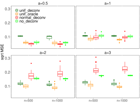
Figure 3: Mean squared errors (square root) obtained with our estimator unif$\_$deconv), with the oracle estimator unif$\_$oracle) for uniform deconvolution, with the fDKDE estimator normal$\_$deconv) and with a density estimator without deconvolution no$\_$deconv) with Epanechnikov kernel. The estimations are provided for 30 simulations in each scenario.

5.3 Computational times

The calibration procedure for the bandwidth selection requires multiple integral computations, in particular if we use a thin grid $\mathcal{H}$. However, the computational times remains reasonable for one estimation especially when the size of the noise is not too small, as summarized in Table 1. The value of $a$ determines indeed the number of non-zero terms in the double sum that appears in the definition of the estimator (3.4) (the smaller $a$, the larger number of terms), which explains that the longest computational times is obtained for the smaller value of $a$ and the larger number of observations $n$. The code, implemented in R, is parallelized and uses the Rcpp package in order to reduce the computational cost.

(a) Beta intensities

	a=0.05	a=0.1
n=500	1123	241
n=1000	4931	1144

(b) Laplace intensities

	a=0.5	a=1	a=2	a=3
n=500	2.79	0.71	0.31	0.29
n=1000	9.76	2.08	0.78	0.76

Table 1: Computational times (in seconds) associated with one estimation for different values of $a$ and $n$ considered in the numerical study. The computations were run on 16 cores of a server Intel Xeon E5-4620 2.20GHz .

6 Deconvolution of Genomic data

Next generation sequencing technologies (NGS) have allowed the fine mapping of eukaryotes replication origins that constitute the starting points of chromosomes duplication. To maintain the stability and integrity of genomes, replication origins are under a very strict spatio-temporal control, and part of their positioning has been shown to be associated with cell differentiation (Picard et al., 2014). The spatial organization has become central to better understand genomes architecture and regulation. However, the positioning of replication origins is subject to errors, since any NGS-based high-throughput mapping consists of peak-calling based on the detection of an exceptional enrichment of short reads Picard et al. (2014). Consequently, the true positions of the replication starting points are unknown, but rather inferred from genomic intervals. The spatial control of replication being very strict, the precise quantification of the density of origins along chromosomes is central, but should account for this imprecision of the mapping step. The interval shape of the data makes the uniform assumption of the noise particularly appropriate. However, other types of distributions could be considered. We compare our results to those obtained by the estimator proposed by Delaigle and Gijbels (2004) and implemented in the R package fDKDE, which was developed to handle errors with Gaussian distribution. Both deconvolution estimators provide an intensity estimation that is less smooth than the one obtained without accounting for the error positioning. However, the estimator of Delaigle and Gijbels (2004) identifies three regions with a high density of origins while ours shows several sharp peaks which suggests the existence of clusters of origins, the location of which can be precisely identified.

The comparison shows that the Gaussian-based estimator is overly smooth regarding the underlying biological process. Indeed, replication origins are known to be organized according to the so-called replication domains that are $\leq 1$Mb on average (Pope et al., 2014). The deconvoluted estimator based on uniform errors provides an intensity that shows peaks that are approximatively $\leq 1$Mb wide, whereas the Gaussian-based estimator shows clusters of size $\sim 3$Mb.

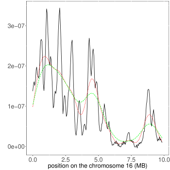
Figure 4: Estimation of the intensity of human replication origins along chromosome 16 ($N^{+}=874$), for 3 procedures: our procedure (Epanechnikov kernel calibrated by our data-driven procedure, black plain line), the two procedures implemented in the fDKDE package (red dashed line) and the procedure implemented in the R density function (Epanechnikov kernel) with the bandwidth calibrated by cross-validation (green dashed line).

In a second step we focused on the spatial distribution of G-quadruplex motifs that were shown to be associated with replication initiation in vertebrates (Picard et al., 2014). Their precise role in replication remains unknown, and their effect may be associated with some epigenetic response (Hänsel-Hertsch et al., 2016) which makes their positional information very valuable regarding the biophysics constraints characterizing the DNA molecule. Thus we considered the spatial distribution of G-quadruplexes (Zheng et al., 2020) along all replication origins (Picard et al., 2014), by considering the initiation peak as the reference position (Figure 5). When estimating the spatial distribution of G-quadruplex motifs around replication origins, the estimator without deconvolution provides an almost flat estimated density with one small central peak. The fDKDE estimator highlights one central peak and several smaller peaks. Finally, our estimator reveals a periodic clustering pattern of G-quadruplexes occurrences along replication origins, which is completely masked when computing a standard density estimator and only slightly suggested with the fDKDE estimator. This clustering pattern could be related to the periodic organization of nucleosomes and chromatin around replication origins as suggested by experimental evidence Prorok et al. (2019). Hence, our estimator provides a finer-scale resolution for the accumulation pattern of G-quadruplexes in the vicinity of replication initiation sites that could be biologically relevant.

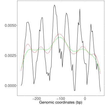
Figure 5: Estimation of the intensity of G-quadruplexes around human replication origins along chromosome 1 ($a=25.9$ the average length of motifs, $N_{+}=2559$) for 3 procedures: our procedure (Epanechnikov kernel calibrated by our data-driven procedure, black plain line), the two procedures implemented in the fDKDE package (red dashed line) and the procedure implemented in the R density function (Epanechnikov kernel) with the bandwidth calibrated by cross-validation (green dashed line). The reference position 0 indicates the position of the replication initiation peak, and we compute the spatial distribution of Gquadruplexes upstream or downstream (negative position values) of origins.

7 Proofs

If $\theta$ is a vector of constants (for instance $\theta=(T,a,K))$, we denote by $\square_{\theta}$ a positive constant that only depends on $\theta$ and that may change from line to line.

In the sequel, we use at several places the following property: Setting

$$S_{k}:\ x\longmapsto\sum_{i=1}^{N_{+}}K_{h}^{\prime}\bigg{(}x-(2k+1)a-Y_{i}\bigg{)},$$

since $Ah\leq a$, $S_{k}$ and $S_{k^{\prime}}$ have disjoint supports if $k\not=k^{\prime}$.

7.1 Proof of Lemma 1

Proof. Considering first $\widehat{f}_{h}$, we have:

$$\mathbb{E}[\widehat{f}_{h}(x)] =\frac{2a}{nh^{2}}\sum_{k=0}^{+\infty}\int_{\mathbb{R}}K^{\prime}\left(\frac{x-(2k+1)a-u}{h}\right)nf_{Y}(u)du$$

$$=\frac{1}{h^{2}}\sum_{k=0}^{+\infty}\int_{\mathbb{R}}K^{\prime}\left(\frac{x-(2k+1)a-u}{h}\right)[F_{X}(u+a)-F_{X}(u-a)]du$$

$$=\frac{1}{h^{2}}\sum_{k=0}^{+\infty}\int_{\mathbb{R}}K^{\prime}\left(\frac{x-2ka-v}{h}\right)F_{X}(v)dv-\int_{\mathbb{R}}K^{\prime}\left(\frac{x-2(k+1)a-v}{h}\right)F_{X}(v)dv$$

$$=\frac{1}{h^{2}}\int_{\mathbb{R}}K^{\prime}\left(\frac{x-v}{h}\right)F_{X}(v)dv$$

$$=\frac{1}{h}\int_{\mathbb{R}}K\left(\frac{x-v}{h}\right)f_{X}(v)dv=(K_{h}\star f_{X})(x).$$

The first point is then straightforward by using the definition of $\widetilde{f}_{h}$. For the second point, observe that

$$\widetilde{f}_{h}(t)-\mathbb{E}[\widetilde{f}_{h}(t)] =\frac{a}{nh^{2}}\sum_{k=-\infty}^{+\infty}s_{k}\int K^{\prime}\left(\frac{t-(2k+1)a-u}{h}\right)\left[dN^{Y}_{u}-nf_{Y}(u)du\right]$$

$$=\frac{a}{nh}\int_{\mathbb{R}}L_{h}(t-u)\left[dN^{Y}_{u}-nf_{Y}(u)du\right],$$

with

$$L_{h}(x):=\frac{1}{h}\sum_{k=-\infty}^{+\infty}s_{k}K^{\prime}\left(\frac{x-(2k+1)a}{h}\right).$$

Using the support $[-A,A]$ of $K$, for each $x$

$$(L_{h}(x))^{2} =\frac{1}{h^{2}}\left(\sum_{k=-\infty}^{+\infty}s_{k}K^{\prime}\left(\frac{x-(2k+1)a}{h}\right)\right)^{2}$$

$$=\frac{1}{h^{2}}\sum_{k=-\infty}^{+\infty}K^{\prime 2}\left(\frac{x-(2k+1)a}{h}\right)$$

as soon as $Ah\leq a$. We have:

$$\int_{0}^{T}\mathbb{E}[(\widetilde{f}_{h}(t)-\mathbb{E}[\widetilde{f}_{h}(t)])^{2}]dt =\frac{a^{2}}{n^{2}h^{2}}\int_{0}^{T}\mathrm{Var}\left(\int_{\mathbb{R}}L_{h}(t-u)dN^{Y}_{u}\right)dt$$

$$=\frac{a^{2}}{n^{2}h^{2}}\int_{0}^{T}\int_{\mathbb{R}}L_{h}^{2}(t-u)nf_{Y}(u)dudt$$

$$=\frac{a^{2}}{nh^{4}}\int_{0}^{T}\int_{\mathbb{R}}\sum_{k=-\infty}^{+\infty}\left(K^{\prime}\left(\frac{t-u-(2k+1)a}{h}\right)\right)^{2}f_{Y}(u)dudt$$

$$=\frac{a^{2}}{nh^{4}}\int_{0}^{T}\int_{\mathbb{R}}\left(K^{\prime}\left(\frac{t-v}{h}\right)\right)^{2}\sum_{k=-\infty}^{+\infty}f_{Y}(v-(2k+1)a)dvdt$$

$$=\frac{a}{2nh^{4}}\int_{0}^{T}\int_{\mathbb{R}}\left(K^{\prime}\left(\frac{t-v}{h}\right)\right)^{2}(\lim_{+\infty}F_{X}-\lim_{-\infty}F_{X})dvdt,$$

which yields

$$\mathbb{E}\Big{[}\|\widetilde{f}_{h}(t)-\mathbb{E}[\widetilde{f}_{h}(t)]\|_{2,T}^{2}\Big{]}=\frac{aT\|f_{X}\|_{1}\|K^{\prime}\|_{2}^{2}}{2nh^{3}}.$$

$\square$

7.2 Auxiliary lemma

Our procedure needs the following result.

Lemma 7

For any $h,t\in\mathcal{H}$,

$$\widetilde{f}_{h,t}=\widetilde{f}_{t,h}.$$

Proof. Since $K_{h}^{\prime}(x)=(1/h^{2})K^{\prime}(x/h)$, we can write

$$K_{h}\star\widehat{f}_{t} =K_{h}\star\left(\frac{2a}{n}\sum_{k=0}^{+\infty}\sum_{i=1}^{N_{+}}(K_{t})^{\prime}({x-(2k+1)a-Y_{i}})\right)$$

$$=\frac{2a}{n}\sum_{k=0}^{+\infty}\sum_{i=1}^{N_{+}}K_{h}\star(K_{t})^{\prime}\left({x-(2k+1)a-Y_{i}}\right)$$

Using that $K_{h}\star(K_{t})^{\prime}=(K_{h}\star K_{t})^{\prime}=(K_{h})^{\prime}\star K_{t}$, we obtain $K_{h}\star\widehat{f}_{t}=K_{t}\star\widehat{f}_{h}$.

In the same way, we can prove $K_{h}\star\check{f}_{t}=K_{t}\star\check{f}_{h}$ and then $K_{h}\star\widetilde{f}_{t}=K_{t}\star\widetilde{f}_{h}$. $\square$

7.3 Proof of Theorem 2

Remember that

$$\hat{h}:=\operatorname*{argmin}_{h\in\mathcal{H}}\left\{{\mathcal{A}}(h)+\frac{c\sqrt{N_{+}}}{nh^{3/2}}\right\},$$

with

$${\mathcal{A}}(h):=\max_{t\in\mathcal{H}}\left\{\|\widetilde{f}_{t}-\widetilde{f}_{h,t}\|_{2,T}-\frac{c\sqrt{N_{+}}}{nt^{3/2}}\right\}_{+}.$$

For any $h\in\mathcal{H}$,

$$\|\widetilde{f}_{\hat{h}}-f_{X}\|_{2,T}\leq A_{1}+A_{2}+A_{3},$$

with

$$A_{1}:=\|\widetilde{f}_{\hat{h}}-\widetilde{f}_{\hat{h},h}\|_{2,T}\leq{\mathcal{A}}(h)+\frac{c\sqrt{N_{+}}}{n\hat{h}^{3/2}},$$

$$A_{2}:=\|\widetilde{f}_{h}-\widetilde{f}_{\hat{h},h}\|_{2,T}\leq{\mathcal{A}}(\hat{h})+\frac{c\sqrt{N_{+}}}{nh^{3/2}},$$

and

$$A_{3}:=\|\widetilde{f}_{h}-f_{X}\|_{2,T}.$$

By definition of $\hat{h}$, we have:

$$A_{1}+A_{2}\leq 2{\mathcal{A}}(h)+\frac{2c\sqrt{N_{+}}}{nh^{3/2}}.$$

Therefore, by setting

$$\zeta_{n}(h):=\sup_{t\in\mathcal{H}}\left\{\|(\widetilde{f}_{t,h}-\mathbb{E}[\widetilde{f}_{t,h}])-(\widetilde{f}_{t}-\mathbb{E}[\widetilde{f}_{t}])\|_{2,T}-\frac{c\sqrt{N_{+}}}{nt^{3/2}}\right\}_{+},$$

we have:

$$A_{1}+A_{2} \leq 2\zeta_{n}(h)+2\sup_{t\in\mathcal{H}}\|\mathbb{E}[\widetilde{f}_{t,h}]-\mathbb{E}[\widetilde{f}_{t}]\|_{2,T}+\frac{2c\sqrt{N_{+}}}{nh^{3/2}}$$

$$\leq 2\zeta_{n}(h)+2\sup_{t\in\mathcal{H}}\|K_{h}\star K_{t}\star f_{X}-K_{t}\star f_{X}\|_{2,T}+\frac{2c\sqrt{N_{+}}}{nh^{3/2}}$$

$$\leq 2\zeta_{n}(h)+2\|K\|_{1}\|K_{h}\star f_{X}-f_{X}\|_{2,T}+\frac{2c\sqrt{N_{+}}}{nh^{3/2}}.$$

Finally, since $(\alpha+\beta+\gamma)^{2}\leq 3\alpha^{2}+3\beta^{2}+3\gamma^{2}$,

$$\mathbb{E}[(A_{1}+A_{2})^{2}] \leq 12\mathbb{E}[\zeta_{n}^{2}(h)]+12\|K\|_{1}^{2}\|K_{h}\star f_{X}-f_{X}\|_{2,T}^{2}+\frac{12c^{2}\mathbb{E}[N_{+}]}{n^{2}h^{3}}$$

$$\leq 12\mathbb{E}[\zeta_{n}^{2}(h)]+12\|K\|_{1}^{2}\|K_{h}\star f_{X}-f_{X}\|_{2,T}^{2}+\frac{12c^{2}\|f_{X}\|_{1}}{nh^{3}}.$$

For the last term, we obtain:

$$\mathbb{E}[A_{3}^{2}] =\mathbb{E}[\|\widetilde{f}_{h}-f_{X}\|_{2,T}^{2}]$$

$$=\mathbb{E}\left[\|\widetilde{f}_{h}-\mathbb{E}[\widetilde{f}_{h}]\|_{2,T}^{2}\right]+\|K_{h}\star f_{X}-f_{X}\|_{2,T}^{2}$$

$$=\frac{aT\|f_{X}\|_{1}\|K^{\prime}\|_{2}^{2}}{2nh^{3}}+\|K_{h}\star f_{X}-f_{X}\|_{2,T}^{2}.$$

Finally, replacing $c$ with its definition, namely

$$c=(1+\eta)(1+\|K\|_{1})\|K^{\prime}\|_{2}\sqrt{\frac{aT}{2}},$$

we obtain: for any $h\in\mathcal{H}$,

$$\mathbb{E}[\|\widetilde{f}_{\hat{h}}-f_{X}\|_{2,T}^{2}] \leq 2\mathbb{E}[(A_{1}+A_{2})^{2}]+2\mathbb{E}[A_{3}^{2}]$$

$$\leq 2(1+12\|K\|_{1}^{2})\|K_{h}\star f_{X}-f_{X}\|_{2,T}^{2}+C_{1}\frac{aT\|f_{X}\|_{1}\|K^{\prime}\|_{2}^{2}}{2nh^{3}}+24\mathbb{E}[\zeta_{n}^{2}(h)]$$

$$\leq C_{1}\mathbb{E}[\|\widetilde{f}_{h}-f_{X}\|_{2,T}^{2}]+24\mathbb{E}[\zeta_{n}^{2}(h)],$$ (7.1)

by using Lemma 1 and by denoting $C_{1}=2+24(1+\eta)^{2}(1+\|K\|_{1})^{2}$. It remains to prove that $\mathbb{E}[\zeta_{n}^{2}(h)]$ is bounded by $\frac{1}{n}$ up to a constant. We have:

$$\zeta_{n}(h) \leq\sup_{t\in\mathcal{H}}\left\{\|\widetilde{f}_{t,h}-\mathbb{E}[\widetilde{f}_{t,h}]\|_{2,T}+\|\widetilde{f}_{t}-\mathbb{E}[\widetilde{f}_{t}]\|_{2,T}-\frac{c\sqrt{N_{+}}}{nt^{3/2}}\right\}_{+}$$

$$\leq\sup_{t\in\mathcal{H}}\left\{(\|K\|_{1}+1)\|\widetilde{f}_{t}-\mathbb{E}[\widetilde{f}_{t}]\|_{2,T}-\frac{c\sqrt{N_{+}}}{nt^{3/2}}\right\}_{+}$$

$$\leq(\|K\|_{1}+1)S_{n},$$

with

$$S_{n}:=\sup_{t\in\mathcal{H}}\left\{\|\widetilde{f}_{t}-\mathbb{E}[\widetilde{f}_{t}]\|_{2,T}-\frac{(1+\eta)\|K^{\prime}\|_{2}\sqrt{aTN_{+}}}{\sqrt{2}nt^{3/2}}\right\}_{+}.$$

For $\alpha\in(0,1)$ chosen later, we compute:

$$A_{n}:=\mathbb{E}[S_{n}^{2}{\bf 1}_{\{N_{+}\leq(1-\alpha)^{2}n\|f_{X}\|_{1}\}}].$$

Recall that (see the proof of Lemma 1)

$$\widetilde{f}_{t}(x)=\frac{a}{nt}\int_{\mathbb{R}}L_{t}(x-u)dN_{u}^{Y},\quad\text{ with }L_{t}(x)=\frac{1}{t}\sum_{k=-\infty}^{\infty}s_{k}K^{\prime}\left(\frac{x-(2k+1)a}{t}\right).$$

Since $At\leq a$,

$$\left(\int_{\mathbb{R}}\sum_{k=-\infty}^{+\infty}s_{k}K^{\prime}\left(\frac{x-(2k+1)a-u}{t}\right)dN^{Y}_{u}\right)^{2} =\left(\sum_{i=1}^{N+}\sum_{k=-\infty}^{\infty}s_{k}K^{\prime}\left(\frac{x-(2k+1)a-Y_{i}}{t}\right)\right)^{2}$$

$$\leq N_{+}\sum_{i=1}^{N+}\sum_{k=-\infty}^{\infty}\left(K^{\prime}\left(\frac{x-(2k+1)a-Y_{i}}{h}\right)\right)^{2}$$

$$\leq N_{+}^{2}\|K^{\prime}\|_{\infty}^{2},$$

which yields

$$S_{n}^{2} \leq 2\sup_{t\in\mathcal{H}}\|\widetilde{f}_{t}\|^{2}_{2,T}+2\sup_{t\in\mathcal{H}}\|\mathbb{E}[\widetilde{f}_{t}]\|^{2}_{2,T}$$

$$\leq\sup_{t\in\mathcal{H}}\frac{2a^{2}}{n^{2}t^{4}}\int_{0}^{T}\left(\int_{\mathbb{R}}\sum_{k=-\infty}^{+\infty}s_{k}K^{\prime}\left(\frac{x-(2k+1)a-u}{t}\right)dN^{Y}_{u}\right)^{2}dx+2\sup_{t\in\mathcal{H}}\|K_{t}\star f_{X}\|^{2}_{2,T}$$

$$\leq\sup_{t\in\mathcal{H}}\frac{2a^{2}\|K^{\prime}\|_{\infty}^{2}TN_{+}^{2}}{n^{2}t^{4}}+2\sup_{t\in\mathcal{H}}\frac{\|K\|^{2}_{2}\|f_{X}\|_{1}^{2}}{t}.$$

Therefore, since $t\in\mathcal{H}\Rightarrow t^{-1}\leq\delta n^{1/3}$,

$$A_{n}\leq\Big{(}2\delta^{4}a^{2}\|K^{\prime}\|_{\infty}^{2}Tn^{4/3}+2\delta\|K\|^{2}_{2}n^{1/3}\Big{)}\|f_{X}\|_{1}^{2}\times\mathbb{P}(N_{+}\leq(1-\alpha)^{2}n\|f_{X}\|_{1}).$$

and since $n\geq 1$

$$A_{n}\leq(2\delta^{4}a^{2}\|K^{\prime}\|_{\infty}^{2}T+2\delta\|K\|_{2}^{2})n^{2}\|f_{X}\|_{1}^{2}\mathbb{P}(N_{+}\leq(1-\alpha)^{2}n\|f_{X}\|_{1}).$$

To bound the last term, we use, for instance, Inequality (5.2) of Reynaud-Bouret (2003) (with $\xi=(2\alpha-\alpha^{2})n\|f_{X}\|_{1}$ and with the function $f\equiv-1$), which shows that there exists $\alpha^{\prime}>0$ only depending on $\alpha$ such that

$$\mathbb{P}(N_{+}\leq(1-\alpha)^{2}n\|f_{X}\|_{1})\leq\exp(-\alpha^{\prime}n\|f_{X}\|_{1}).$$

This shows that there exists a positive constant $C_{\alpha}$ such that

$$A_{n}\leq(2\delta^{4}a^{2}\|K^{\prime}\|_{\infty}^{2}T+2\delta\|K\|_{2}^{2})\frac{C_{\alpha}}{n\|f_{X}\|_{1}}.$$

We now deal with

$$B_{n}:=\mathbb{E}[S_{n}^{2}{\bf 1}_{\{N_{+}>(1-\alpha)^{2}n\|f_{X}\|_{1}\}}].$$

We take $\alpha=\min(\eta/2,1/4)$. This implies

$$(1+\eta)(1-\alpha)\geq 1+\frac{\eta}{4}$$

and

$$B_{n} =\mathbb{E}\left[\sup_{t\in\mathcal{H}}\left\{\|\widetilde{f}_{t}-\mathbb{E}[\widetilde{f}_{t}]\|_{2,T}-\frac{(1+\eta)\|K^{\prime}\|_{2}\sqrt{aTN_{+}}}{\sqrt{2}nt^{3/2}}\right\}_{+}^{2}{\bf 1}_{\{N_{+}>(1-\alpha)^{2}n\|f_{X}\|_{1}\}}\right]$$

$$\leq\mathbb{E}\left[\sup_{t\in\mathcal{H}}\left\{\|\widetilde{f}_{t}-\mathbb{E}[\widetilde{f}_{t}]\|_{2,T}-\frac{(1+\eta/4)\sqrt{aT}\|K^{\prime}\|_{2}\sqrt{\|f_{X}\|_{1}}}{\sqrt{2n}t^{3/2}}\right\}_{+}^{2}\right]$$

$$\leq\int_{0}^{+\infty}\mathbb{P}\left(\sup_{t\in\mathcal{H}}\left\{\|\widetilde{f}_{t}-\mathbb{E}[\widetilde{f}_{t}]\|_{2,T}-\frac{(1+\eta/4)\sqrt{aT}\|K^{\prime}\|_{2}\sqrt{\|f_{X}\|_{1}}}{\sqrt{2n}t^{3/2}}\right\}_{+}^{2}\geq x\right)dx$$

$$\leq\sum_{t\in\mathcal{H}}\int_{0}^{+\infty}\mathbb{P}\left(\left\{\|\widetilde{f}_{t}-\mathbb{E}[\widetilde{f}_{t}]\|_{2,T}-\frac{(1+\eta/4)\sqrt{aT}\|K^{\prime}\|_{2}\sqrt{\|f_{X}\|_{1}}}{\sqrt{2n}t^{3/2}}\right\}_{+}^{2}\geq x\right)dx.$$

To conclude, it remains to control for any $x>0$ the probability inside the integral. For this purpose, we use the following lemma.

Lemma 8

Let $\varepsilon>0$ and $h\in\mathcal{H}$ be fixed. For any $x>0$, with probability larger than $1-\exp(-x)$,

$$\|\widetilde{f}_{h}-\mathbb{E}[\widetilde{f}_{h}]\|_{2,T}\leq(1+\varepsilon)\|K^{\prime}\|_{2}\sqrt{\frac{aT\|f_{X}\|_{1}}{2nh^{3}}}+\sqrt{12x}\|K^{\prime}\|_{1}\sqrt{\frac{\|f_{X}\|_{1}(T+4a)}{4nh^{2}}}+(1.25+32\varepsilon^{-1})x\frac{\|K^{\prime}\|_{2}}{nh^{3/2}}\sqrt{\frac{a(T+4a)}{2}}.$$

Proof. We set:

$$U(t) =\widetilde{f}_{h}(t)-\mathbb{E}[\widetilde{f}_{h}(t)]$$

$$=\frac{a}{nh^{2}}\sum_{k=-\infty}^{+\infty}s_{k}\int_{\mathbb{R}}K^{\prime}\left(\frac{t-(2k+1)a-u}{h}\right)\left[dN^{Y}_{u}-nf_{Y}(u)du\right]$$

$$=\frac{a}{nh}\int_{\mathbb{R}}L_{h}(t-u)\left[dN^{Y}_{u}-nf_{Y}(u)du\right],$$

with

$$L_{h}(x):=\frac{1}{h}\sum_{k=-\infty}^{+\infty}s_{k}K^{\prime}\left(\frac{x-(2k+1)a}{h}\right).$$

Let $\mathcal{D}$ a countable dense subset of the unit ball of ${\mathbb{L}}_{2}[0,T]$. We have:

$$\|U\|_{2,T} =\sup_{g\in\mathcal{D}}\int_{0}^{T}g(t)U(t)dt$$

$$=\sup_{g\in\mathcal{D}}\int_{\mathbb{R}}\Psi_{g}(u)\left[dN^{Y}_{u}-nf_{Y}(u)du\right],$$

with

$$\Psi_{g}(u):=\frac{a}{nh}\int_{0}^{T}L_{h}(t-u)g(t)dt=\frac{a}{nh}(\widetilde{L}_{h}\star g)(u)$$

and $\widetilde{L}_{h}(x)=L_{h}(-x)$, where the convolution product is computed on $[0,T]$. We use Corollary 2 of Reynaud-Bouret (2003). So, we need to bound $\mathbb{E}[\|U\|_{2,T}]$ and

$$v_{0}:=\sup_{g\in\mathcal{D}}\int_{\mathbb{R}}\Psi_{g}^{2}(u)nf_{Y}(u)du.$$

We also have to determine $b$, a deterministic upper bound for all the $\Psi_{g}$’s. We have already proved in the proof of Lemma 1 that

$$\mathbb{E}[\|U\|_{2,T}^{2}] =\frac{aT\|f_{X}\|_{1}\|K^{\prime}\|_{2}^{2}}{2nh^{3}},$$

which implies

$$\mathbb{E}[\|U\|_{2,T}]\leq\|K^{\prime}\|_{2}\sqrt{\frac{aT\|f_{X}\|_{1}}{2nh^{3}}}.$$ (7.2)

If we denote $I(h,u):=\{k\in\mathbb{Z}:-u-Ah-a\leq 2ka\leq Ah+T-u-a\},$ then

$$\Psi_{g}^{2}(u) =\frac{a^{2}}{n^{2}h^{2}}\left(\int_{0}^{T}L_{h}(t-u)g(t)dt\right)^{2}$$

$$\leq\frac{a^{2}}{n^{2}h^{2}}\int_{0}^{T}L_{h}^{2}(t-u)dt\times\int_{0}^{T}g^{2}(t)dt$$

$$\leq\frac{a^{2}}{n^{2}h^{4}}\int_{0}^{T}\sum_{k\in I(h,u)}\left(K^{\prime}\left(\frac{t-u-(2k+1)a}{h}\right)\right)^{2}dt$$

$$\leq\frac{a^{2}}{n^{2}h^{3}}\|K^{\prime}\|_{2}^{2}\times\mbox{card}(I(h,u))$$

$$\leq\frac{a^{2}}{n^{2}h^{3}}\|K^{\prime}\|_{2}^{2}\times(T/(2a)+Ah/a+1)$$

and we can set, under the condition on $\mathcal{H}$,

$$b:=\frac{a}{nh^{3/2}}\|K^{\prime}\|_{2}\sqrt{\frac{T+4a}{2a}},$$

which is negligible with respect to the upper bound of $\mathbb{E}[\|U\|_{2,T}]$ given in (7.2). We now deal with

$$v_{0}:=n\times\sup_{g\in\mathcal{D}}\int_{\mathbb{R}}\Psi_{g}^{2}(u)f_{Y}(u)du.$$

We have:

$$v_{0} =\frac{a^{2}}{nh^{2}}\sup_{g\in\mathcal{D}}\int_{\mathbb{R}}\left(\int_{0}^{T}L_{h}(t-u)g(t)dt\right)^{2}f_{Y}(u)du$$

$$\leq\frac{a^{2}}{nh^{2}}\sup_{g\in\mathcal{D}}\int_{\mathbb{R}}\left(\int_{0}^{T}|L_{h}(t-u)|dt\int_{0}^{T}|L_{h}(t-u)|g^{2}(t)dt\right)f_{Y}(u)du.$$

Since

$$\int_{0}^{T}|L_{h}(t-u)|dt \leq\frac{1}{h}\int_{0}^{T}\sum_{k\in I(h,u)}\left|K^{\prime}\left(\frac{t-u-(2k+1)a}{h}\right)\right|dt$$

$$\leq\|K^{\prime}\|_{1}\mbox{card}(I(h,u))$$

$$\leq\|K^{\prime}\|_{1}\frac{(T+4a)}{2a},$$

we obtain

$$v_{0} \leq\frac{a^{2}}{nh^{2}}\|K^{\prime}\|_{1}\frac{(T+4a)}{2a}\sup_{g\in\mathcal{D}}\int_{\mathbb{R}}\int_{0}^{T}\sum_{k=-\infty}^{+\infty}\frac{1}{h}\left|K^{\prime}\left(\frac{t-u-(2k+1)a}{h}\right)\right|g^{2}(t)dtf_{Y}(u)du$$

$$\leq\frac{a}{2nh^{2}}\|K^{\prime}\|_{1}(T+4a)\sup_{g\in\mathcal{D}}\int_{0}^{T}\left(\int\frac{1}{h}\left|K^{\prime}\left(\frac{t-v}{h}\right)\right|\sum_{k=-\infty}^{+\infty}f_{Y}(v-(2k+1)a)dv\right)g^{2}(t)dt$$

$$\leq\frac{a}{2nh^{2}}\|K^{\prime}\|_{1}(T+4a)\sup_{g\in\mathcal{D}}\int_{0}^{T}\left(\int\frac{1}{h}\left|K^{\prime}\left(\frac{t-v}{h}\right)\right|dv\right)\frac{\|f_{X}\|_{1}}{2a}g^{2}(t)dt$$

$$\leq\frac{\|f_{X}\|_{1}}{4nh^{2}}\|K^{\prime}\|_{1}^{2}(T+4a).$$

Inequality (5.7) of Reynaud-Bouret (2003) yields, for any $x>0$,

$$\mathbb{P}\left(\|U\|_{2,T}\geq(1+\varepsilon)\mathbb{E}[\|U\|_{2,T}]+\sqrt{12v_{0}x}+(1.25+32\varepsilon^{-1})bx\right)\leq\exp(-x).$$

Setting

$$RHS :=(1+\varepsilon)\mathbb{E}[\|U\|_{2,T}]+\sqrt{12v_{0}x}+(1.25+32\varepsilon^{-1})bx,$$

we obtain

$$RHS \leq(1+\varepsilon)\|K^{\prime}\|_{2}\sqrt{\frac{aT\|f_{X}\|_{1}}{2nh^{3}}}+\sqrt{12x}\|K^{\prime}\|_{1}\sqrt{\frac{\|f_{X}\|_{1}(T+4a)}{4nh^{2}}}+(1.25+32\varepsilon^{-1})x\frac{\|K^{\prime}\|_{2}}{nh^{3/2}}\sqrt{\frac{a(T+4a)}{2}}.$$

$\square$

The previous lemma states that for any sequence of weights $(w_{h})_{h\in{\mathcal{H}}}$, setting $x=w_{h}+u$, with $u>0$, with probability larger than $1-\exp(-u)\sum_{h\in{\mathcal{H}}}\exp(-w_{h})$, for all $h\in\mathcal{H}$,

$$\|\widetilde{f}_{h}-\mathbb{E}[\widetilde{f}_{h}]\|_{2,T}\leq M_{h}+\sqrt{12u}\|K^{\prime}\|_{1}\sqrt{\frac{\|f_{X}\|_{1}(T+4a)}{4nh^{2}}}+(1.25+32\varepsilon^{-1})u\frac{\|K^{\prime}\|_{2}}{nh^{3/2}}\sqrt{\frac{a(T+4a)}{2}}$$

with

$$M_{h} :=(1+\varepsilon)\|K^{\prime}\|_{2}\sqrt{\frac{aT\|f_{X}\|_{1}}{2nh^{3}}}+\sqrt{12w_{h}}\|K^{\prime}\|_{1}\sqrt{\frac{\|f_{X}\|_{1}(T+4a)}{4nh^{2}}}+(1.25+32\varepsilon^{-1})w_{h}\frac{\|K^{\prime}\|_{2}}{nh^{3/2}}\sqrt{\frac{a(T+4a)}{2}}$$

$$=\|K^{\prime}\|_{2}\sqrt{\frac{aT\|f_{X}\|_{1}}{2nh^{3}}}\left(1+\varepsilon+\sqrt{12w_{h}h}\frac{\|K^{\prime}\|_{1}}{\|K^{\prime}\|_{2}}\frac{\sqrt{T+4a}}{\sqrt{2aT}}+\frac{(1.25+32\varepsilon^{-1})w_{h}}{\sqrt{n\|f_{X}\|_{1}}}\sqrt{\frac{T+4a}{T}}\right)$$

$$\leq\frac{(1+\eta/4)\sqrt{aT}\|K^{\prime}\|_{2}\sqrt{\|f_{X}\|_{1}}}{\sqrt{2n}h^{3/2}},$$

for $\varepsilon=\eta/8$ and for $n$ large enough, by taking $w_{h}=h^{-1/2}|\log h|^{-1}$ for instance, since in this case,

$$w_{h}h=o(1)\quad\mbox{and}\quad h^{-1}=O(n\|f_{X}\|_{1}).$$

Therefore,

$$B_{n} \leq\sum_{h\in\mathcal{H}}\int_{0}^{+\infty}\mathbb{P}\left(\left\{\|\widetilde{f}_{h}-\mathbb{E}[\widetilde{f}_{h}]\|_{2,T}-M_{h}\right\}_{+}^{2}\geq x\right)dx.$$

By setting $u$ such that

$$x:=(g(u))^{2}=\left(\sqrt{12u}\|K^{\prime}\|_{1}\sqrt{\frac{\|f_{X}\|_{1}(T+4a)}{4nh^{2}}}+(1.25+32\varepsilon^{-1})u\frac{\|K^{\prime}\|_{2}}{nh^{3/2}}\sqrt{\frac{a(T+4a)}{2}}\right)^{2},$$

so

$$dx=2g(u)\times\left(\frac{\sqrt{12}}{2\sqrt{u}}\|K^{\prime}\|_{1}\sqrt{\frac{\|f_{X}\|_{1}(T+4a)}{4nh^{2}}}+(1.25+32\varepsilon^{-1})\frac{\|K^{\prime}\|_{2}}{nh^{3/2}}\sqrt{\frac{a(T+4a)}{2}}\right)du$$

and using that $\int_{0}^{\infty}e^{-u}(D\sqrt{u}+Eu)^{2}u^{-1}du\leq 2D^{2}+2E^{2}$, we obtain

$$B_{n} \leq\sum_{h\in\mathcal{H}}\int_{0}^{+\infty}e^{-(w_{h}+u)}\times 2g(u)\times\left(\frac{\sqrt{12}}{2\sqrt{u}}\|K^{\prime}\|_{1}\sqrt{\frac{\|f_{X}\|_{1}(T+4a)}{4nh^{2}}}+(1.25+32\varepsilon^{-1})\frac{\|K^{\prime}\|_{2}}{nh^{3/2}}\sqrt{\frac{a(T+4a)}{2}}\right)du$$

$$\leq 2\sum_{h\in\mathcal{H}}e^{-w_{h}}\int_{0}^{+\infty}e^{-u}(g(u))^{2}u^{-1}du$$

$$\leq 4\sum_{h\in\mathcal{H}}e^{-w_{h}}\left(12\|K^{\prime}\|_{1}^{2}\frac{\|f_{X}\|_{1}(T+4a)}{4nh^{2}}+(1.25+32\varepsilon^{-1})^{2}\frac{\|K^{\prime}\|_{2}^{2}}{n^{2}h^{3}}{\frac{a(T+4a)}{2}}\right).$$

Since $\sum_{h\in\mathcal{H}}e^{-w_{h}}h^{-2}$ and $\sum_{h\in\mathcal{H}}e^{-w_{h}}h^{-3}$ are bounded by an absolute constant, say $C$, we can write, still for $\varepsilon=\eta/8$,

$$B_{n} \leq 4C\left(12\|K^{\prime}\|_{1}^{2}\frac{\|f_{X}\|_{1}(T+4a)}{4n}+(1.25+32(\eta/8)^{-1})^{2}\frac{\|K^{\prime}\|_{2}^{2}}{n^{2}}{\frac{a(T+4a)}{2}}\right)$$

$$\leq 12C\|K^{\prime}\|_{1}^{2}(T+4a)\frac{\|f_{X}\|_{1}}{n}+2C(1.25+256/\eta)^{2}\|K^{\prime}\|_{2}^{2}a(T+4a)\frac{1}{n^{2}}.$$

Finally, we obtain

$$\mathbb{E}[\zeta_{n}^{2}(h)]\leq(\|K\|_{1}+1)^{2}\mathbb{E}[S_{n}^{2}]\leq(\|K\|_{1}+1)^{2}\left(\frac{c_{1}}{n\|f_{X}\|_{1}}+\frac{c_{2}\|f_{X}\|_{1}}{n}+\frac{c_{3}}{n^{2}}\right),$$

with $c_{1}=C_{\alpha}(2\delta^{4}a^{2}\|K^{\prime}\|_{\infty}^{2}T+2\delta\|K\|_{2}^{2})$, $c_{2}=12C\|K^{\prime}\|_{1}^{2}(T+4a)$ and $c_{3}=2C(1.25+256/\eta)^{2}\|K^{\prime}\|_{2}^{2}a(T+4a).$ This concludes the proof of the theorem, with

$$C_{2}=(\|K\|_{1}+1)^{2}\left(c_{1}\|f_{X}\|_{1}^{-1}+{c_{2}\|f_{X}\|_{1}}+c_{3}\right).$$ (7.3)

7.4 Proof of Theorem 5

To prove Theorem 5, without loss of generality, we assume that $T$ is a positive integer. We denote $a\wedge b=\min(a,b)$ and $a\vee b=\max(a,b)$. The cardinal of a finite set $m$ is denoted by $|m|$.

As usual in the proofs of lower bounds, we build a set of intensities $(f_{m})_{m\in\mathcal{M}}$ quite distant from each other in terms of the ${\mathbb{L}}_{2}$-norm, but whose distance between the resulting models is small. This set of intensities is based on wavelet expansions. More precisely, let $\psi$ be the Meyer wavelet built with with $C^{2}$-conjugate mirror filters (see for instance Section 7.7.2 of Mallat (2009)). We shall use in particular that $\psi$ is $C^{\infty}$ and there exists a positive constant $c_{\psi}$ such that

1. $|\psi(x)|\leq c_{\psi}(1+|x|)^{-2}$ for any $x\in\mathbb{R}$,

2. $\psi^{*}$ is $C^{2}$ and $\psi^{*}$ has support included into $[-8\pi/3,-2\pi/3]\cup[2\pi/3,8\pi/3]$,

where $\psi^{*}(\xi)=\int e^{it\xi}\psi(x)dx$ is the Fourier transform of $\psi$. Observe that this implies that the functions

$$\xi\mapsto\psi^{*}(\xi),\quad\xi\mapsto\psi^{*}(\xi)\xi^{-1},\quad\xi\mapsto\psi^{*}(\xi)\xi^{-2},\quad\xi\mapsto(\psi^{*})^{\prime}(\xi)\quad\mbox{and}\quad\xi\mapsto(\psi^{*})^{\prime}(\xi)\xi^{-1}$$

are bounded by a constant. Without loss of generality, we assume that this constant is $c_{\psi}$.

Let

$$f_{1}(x)=\frac{c_{1}}{1+x^{2}},$$

where $c_{1}$ is a positive constant small enough, which is chosen such that $f_{1}$ belongs to ${\mathcal{S}}^{\beta}(L/2)$, where we denote

$${\mathcal{S}}^{\beta}(L):={\mathcal{S}}^{\beta}(L,0,+\infty)=\left\{g\in\mathbb{L}_{2}:\quad\int_{-\infty}^{+\infty}|g^{*}(\xi)|^{2}(\xi^{2}+1)^{\beta}d\xi\leq L^{2}\right\}.$$

Indeed, note that

$${\mathfrak{c}_{\beta}}^{2}:=\int|c_{1}^{-1}f_{1}^{*}(\xi)|^{2}(\xi^{2}+1)^{\beta}=\int\pi^{2}\exp(-2|\xi|)(\xi^{2}+1)^{\beta}<\infty$$ (7.4)

so that it is sufficient to choose $c_{1}=\mathfrak{c}_{\beta}^{-1}L/2$. With this choice we also have $r\leq\|f_{1}\|_{1}=c_{1}\pi\leq bL$ since we have assumed $rL^{-1}\leq\pi/(2\mathfrak{c}_{\beta})\leq b$; then $f_{1}\in{\mathcal{S}}^{\beta}(L/2,r,b)$.

We recall a combinatorial lemma due to Birgé and Massart (see Lemma 8 in Reynaud-Bouret (2003), see also Lemma 2.9 in Tsybakov (2008)).

Lemma 9

Let $D$ an integer and $\varGamma$ be a finite set with cardinal $D$. There exist absolute constants $\tau$ and $\sigma$ such that there exists $\mathcal{M}_{D}\subset\mathcal{P}(\varGamma)$, satisfying $\log|\mathcal{M}_{D}|\geq\sigma D$ and such that for all distinct sets $m$ and $m^{\prime}$ belonging to $\mathcal{M}_{D}$ the symmetric difference of $m$ and $m^{\prime}$, denoted $m\Delta m^{\prime}$, satisfies $|m\Delta m^{\prime}|\geq\tau D$.

Here we choose $\varGamma:=\{0,\dots,D-1\}$ with $D:=T2^{j-1}$ where $j$ is an integer to be chosen later (so, we take $T2^{j-1}\geq 1$), and we denote $\mathcal{M}:=\mathcal{M}_{D}$ given in the previous lemma. Thus $\log|\mathcal{M}|\geq\sigma T2^{j-1}$ and for all $m,m^{\prime}\in\mathcal{M}$ : $\tau T2^{j-1}\leq|m\Delta m^{\prime}|\leq T2^{j-1}$.

Now, for $a_{j}>0$ to be chosen, for $m\in\mathcal{M}$, for $x\in\mathbb{R}$, we set

$$f_{m}(x):=f_{1}(x)+a_{j}\sum_{k\in m}\psi_{jk}(x),$$

where we have denoted, as usual, $\psi_{jk}(x):=2^{j/2}\psi(2^{j}x-k)$.

We compute $\psi_{jk}^{*}(\xi)=2^{-j/2}e^{i\xi k2^{-j}}\psi^{*}(\xi 2^{-j}),$ which gives

$$\int|(f_{m}-f_{1})^{*}(\xi)|^{2}(1+\xi^{2})^{\beta}d\xi =\int\left|a_{j}2^{-j/2}\psi^{*}(\xi 2^{-j})\sum_{k\in m}e^{i\xi k2^{-j}}\right|^{2}(1+\xi^{2})^{\beta}d\xi$$

$$=a_{j}^{2}\int\left|\psi^{*}(t)\sum_{k\in m}e^{ikt}\right|^{2}(1+t^{2}2^{2j})^{\beta}dt$$

$$\leq\square_{\psi,\beta}a_{j}^{2}2^{2j\beta}\int_{-3\pi}^{3\pi}\left|\sum_{k\in m}e^{ikt}\right|^{2}dt$$

$$\leq\square_{\psi,\beta}2^{2j\beta}|m|a_{j}^{2}\leq\square_{\psi,\beta}T2^{j(2\beta+1)}a_{j}^{2},$$

using Parseval’s theorem and $|m|\leq D=T2^{j-1}$. We assume from now on that

$$T2^{j(2\beta+1)}a_{j}^{2}\leq C(\psi,\beta)L^{2}$$ (7.5)

for $C(\psi,\beta)$ a constant only depending on $\beta$ and $L$ small enough, so that $(f_{m}-f_{1})$ belongs to ${\mathcal{S}}^{\beta}(L/2)$ and then $f_{m}\in{\mathcal{S}}^{\beta}(L)$.

Let us verify that $f_{m}$ is non-negative, and then is an intensity of a Poisson process. Since $\|f_{m}\|_{1}=\int f_{m}(x)dx=\|f_{1}\|_{1}\in[r;bL]$, this will also ensure that $f_{m}\in{\mathcal{S}}^{\beta}(L,r,b)$. For any real $x$,

$$\frac{f_{m}(x)-f_{1}(x)}{f_{1}(x)} =c_{1}^{-1}(1+x^{2})a_{j}2^{j/2}\sum_{k\in m}\psi(2^{j}x-k).$$

Recall that $\psi(x)\leq c_{\psi}(1+|x|)^{-2}$. Let us now study 3 cases.

1. If $0\leq|x|\leq T+1$, we have:

   $$(1+x^{2})\left|\sum_{k\in m}\psi(2^{j}x-k)\right|\leq(T^{2}+2T+2)c_{\psi}\sum_{k\in m}(1+|2^{j}x-k|)^{-2}\leq 2c_{\psi}(T^{2}+2T+2)\sum_{\ell=1}^{+\infty}\ell^{-2},$$

   and the last upper bound is smaller than a finite constant only depending on $T$ and $c_{\psi}$.

2. If $x\geq T+1$, since $|m|\leq D=T2^{j-1}$, we have:

   $$(1+x^{2})\left|\sum_{k\in m}\psi(2^{j}x-k)\right|\leq c_{\psi}T2^{j-1}(1+2^{j}(x-T))^{-2}(1+x^{2})\leq c_{\psi}T2^{-j-1}\sup_{x\geq T+1}\frac{1+x^{2}}{(x-T)^{2}},$$

   and the last expression is smaller than a finite constant only depending on $T$ and $c_{\psi}$.

3. If $x\leq-T-1$,

   $$(1+x^{2})\left|\sum_{k\in m}\psi(2^{j}x-k)\right|\leq c_{\psi}T2^{j-1}(1+2^{j}(-x))^{-2}(1+x^{2})\leq c_{\psi}T2^{-j-1}\sup_{x\leq-T-1}\frac{1+x^{2}}{(-x)^{2}},$$

Finally we obtain that there exists $\bar{C}(T,c_{\psi})$ a constant only depending on $T$ and $c_{\psi}$ such that

$$\frac{|f_{m}(x)-f_{1}(x)|}{f_{1}(x)} \leq c_{1}^{-1}a_{j}2^{j/2}\bar{C}(T,c_{\psi}).$$

We take $a_{j}$ such that

$$c_{1}^{-1}a_{j}2^{j/2}\bar{C}(T,c_{\psi})\leq\frac{1}{2}.$$ (7.6)

This ensures that $f_{m}\geq\frac{1}{2}f_{1}\geq 0.$ Another consequence is that $f_{\varepsilon}\star f_{m}\geq\frac{1}{2}f_{\varepsilon}\star f_{1}$. This provides

$$f_{\varepsilon}\star f_{m}(x) \geq\frac{1}{2}\int_{-a}^{a}\frac{1}{2a}\frac{c_{1}}{1+(x-t)^{2}}dt\geq\frac{1}{2}\>\frac{c_{1}}{1+(|x|+a)^{2}}$$

$$\geq\frac{1}{2}\>\frac{c_{1}}{1+2a^{2}+2x^{2}}\geq\frac{c_{2}^{-1}}{1+x^{2}},$$

denoting $c_{2}=c_{2}(a,\beta,L)=\max(4,2+4a^{2})/c_{1}$.

Finally, we evaluate the distance between the distributions of the observations $N^{Y}$ when $N^{X}$ has intensity $nf_{m}$ and $nf_{m^{\prime}}$. We denote by $\mathbb{P}_{m}$ the probability measure associated with $N^{Y}$, which has intensity $g_{m}:=f_{\varepsilon}\star nf_{m}$, and we denote by $K(\mathbb{P}_{m},\mathbb{P}_{m^{\prime}})$ the Kullback-Leibler divergence between $\mathbb{P}_{m}$ and $\mathbb{P}_{m^{\prime}}$. Using Cavalier and Koo (2002), we have

$$K(\mathbb{P}_{m},\mathbb{P}_{m^{\prime}})=\int g_{m}(x)\phi\left(\log\left(\frac{g_{m^{\prime}}(x)}{g_{m}(x)}\right)\right)dx$$

where for any $x\in\mathbb{R}$, $\phi(x)=\exp(x)-x-1.$ Since for any $x>-1,$ $\log(1+x)\geq x/(1+x)$, we have

$$K(\mathbb{P}_{m},\mathbb{P}_{m^{\prime}})\leq\int\frac{(g_{m}(x)-g_{m^{\prime}}(x))^{2}}{g_{m}(x)}dx=n\int\frac{((f_{\varepsilon}\star f_{m})(x)-(f_{\varepsilon}\star f_{m^{\prime}})(x))^{2}}{(f_{\varepsilon}\star f_{m})(x)}dx.$$

For $m$ and $m^{\prime}$ in $\mathcal{M}$, denote

$$\theta(x)=a_{j}^{-1}(f_{\varepsilon}\star(f_{m}-f_{m^{\prime}}))(x)=\sum_{k\in m\Delta m^{\prime}}b_{k}(f_{\varepsilon}\star\psi_{jk})(x)$$

with $b_{k}=1$ if $k\in m$ and $b_{k}=-1$ if $k\in m^{\prime}$. Denote also $\theta^{*}(\xi)=\int e^{i\xi x}\theta(x)dx$ its Fourier transform, and $(\theta^{*})^{\prime}(\xi)=\int ixe^{i\xi x}\theta(x)dx$ the derivative of $\theta^{*}$. Parseval’s theorem gives

$$\|\theta\|_{2}^{2}=\frac{1}{2\pi}\|\theta^{*}\|_{2}^{2},\quad\text{ and }\|x\theta(x)\|_{2}^{2}=\frac{1}{2\pi}\|(\theta^{*})^{\prime}\|_{2}^{2}.$$

Thus

$$\frac{1}{n}K(\mathbb{P}_{m},\mathbb{P}_{m^{\prime}}) \leq\int\frac{((f_{\varepsilon}\star f_{m})(x)-(f_{\varepsilon}\star f_{m^{\prime}})(x))^{2}}{(f_{\varepsilon}\star f_{m})(x)}dx\leq c_{2}\int(1+x^{2})(f_{\varepsilon}\star(f_{m}-f_{m^{\prime}})(x))^{2}dx$$

$$\leq c_{2}a_{j}^{2}\int(1+x^{2})\theta(x)^{2}dx\leq\frac{c_{2}}{2\pi}a_{j}^{2}\left(\|\theta^{*}\|_{2}^{2}+\|(\theta^{*})^{\prime}\|_{2}^{2}\right).$$

We recall that $\psi_{jk}^{*}(\xi)=2^{-j/2}e^{i\xi k2^{-j}}\psi^{*}(\xi 2^{-j}),$ which gives

$$\theta^{*}(\xi) =\sum_{k\in m\Delta m^{\prime}}b_{k}f_{\varepsilon}^{*}(\xi)\psi_{jk}^{*}(\xi)=\sum_{k\in m\Delta m^{\prime}}b_{k}f_{\varepsilon}^{*}(\xi)2^{-j/2}e^{i\xi k2^{-j}}\psi^{*}(\xi 2^{-j})$$

$$=2^{-j/2}f_{\varepsilon}^{*}(\xi)\psi^{*}(\xi 2^{-j})\sum_{k\in m\Delta m^{\prime}}b_{k}e^{i\xi k2^{-j}}.$$

Thus, remembering that for $\xi\in\mathbb{R},$

$$|f_{\varepsilon}^{*}(\xi)|=\left|\frac{\sin(a\xi)}{a\xi}\right|\leq\min(1,|a\xi|^{-1}),$$ (7.7)

we have

$$\|\theta^{*}\|_{2}^{2} =\int\left|2^{-j/2}f_{\varepsilon}^{*}(\xi)\psi^{*}(\xi 2^{-j})\sum_{k\in m\Delta m^{\prime}}b_{k}e^{i\xi k2^{-j}}\right|^{2}d\xi$$

$$=\int\left|f_{\varepsilon}^{*}(u2^{j})\psi^{*}(u)\sum_{k\in m\Delta m^{\prime}}b_{k}e^{iku}\right|^{2}du$$

$$\leq\int\min(1,|a2^{j}u|^{-2}){|\psi^{*}(u)|^{2}}\left|\sum_{k\in m\Delta m^{\prime}}b_{k}e^{iku}\right|^{2}du$$

$$\leq\int_{-8\pi/3}^{8\pi/3}\min(1,|a2^{j}|^{-2})c_{\psi}^{2}\left|\sum_{k\in m\Delta m^{\prime}}b_{k}e^{iku}\right|^{2}du$$

using the properties of $\psi$. Parseval’s theorem gives

$$\frac{1}{2\pi}\int_{-\pi}^{\pi}\left|\sum_{k\in m\Delta m^{\prime}}b_{k}e^{iku}\right|^{2}du=\sum_{k\in m\Delta m^{\prime}}b_{k}^{2}=|m\Delta m^{\prime}|\leq T2^{j-1}.$$

Then

$$\|\theta^{*}\|_{2}^{2}\leq 3\pi c_{\psi}^{2}T2^{j}(a^{-2}2^{-2j}\wedge 1).$$

Let us now bound $\|(\theta^{*})^{\prime}\|_{2}^{2}$. First

$$(\psi_{jk}^{*})^{\prime}(\xi)=2^{-3j/2}e^{i\xi k2^{-j}}\left(\psi^{*}(\xi 2^{-j})ik+(\psi^{*})^{\prime}(\xi 2^{-j})\right),$$

then

$$(\theta^{*})^{\prime}(\xi) =\sum_{k\in m\Delta m^{\prime}}b_{k}\left[(f_{\varepsilon}^{*})^{\prime}(\xi)\psi_{jk}^{*}(\xi)+f_{\varepsilon}^{*}(\xi)(\psi_{jk}^{*})^{\prime}(\xi)\right]$$

$$=\sum_{k\in m\Delta m^{\prime}}b_{k}(f_{\varepsilon}^{*})^{\prime}(\xi)2^{-j/2}e^{i\xi k2^{-j}}\psi^{*}(\xi 2^{-j})+b_{k}f_{\varepsilon}^{*}(\xi)2^{-3j/2}e^{i\xi k2^{-j}}\left(\psi^{*}(\xi 2^{-j})ik+(\psi^{*})^{\prime}(\xi 2^{-j})\right)$$

$$=\alpha_{1}(\xi)+\alpha_{2}(\xi)+\alpha_{3}(\xi)$$

where

$$\alpha_{1}(\xi)=2^{-j/2}(f_{\varepsilon}^{*})^{\prime}(\xi)\psi^{*}(\xi 2^{-j})\sum_{k\in m\Delta m^{\prime}}b_{k}e^{i\xi k2^{-j}},$$

$$\alpha_{2}(\xi)=2^{-3j/2}f_{\varepsilon}^{*}(\xi)\psi^{*}(\xi 2^{-j})\sum_{k\in m\Delta m^{\prime}}ikb_{k}e^{i\xi k2^{-j}},$$

$$\alpha_{3}(\xi)=2^{-3j/2}f_{\varepsilon}^{*}(\xi)(\psi^{*})^{\prime}(\xi 2^{-j})\sum_{k\in m\Delta m^{\prime}}b_{k}e^{i\xi k2^{-j}}.$$

Reasoning as before, and using that

$$|(f_{\varepsilon}^{*})^{\prime}(\xi)|=\left|\frac{\cos(a\xi)}{\xi}-\frac{1}{\xi}\times\frac{\sin(a\xi)}{a\xi}\right|\leq\frac{2}{|\xi|},$$ (7.8)

we can write

$$\|\alpha_{1}\|_{2}^{2} =\int\left|(f_{\varepsilon}^{*})^{\prime}(u2^{j})\psi^{*}(u)\sum_{k\in m\Delta m^{\prime}}b_{k}e^{iku}\right|^{2}du$$

$$\leq\int\frac{4}{u^{2}2^{2j}}|\psi^{*}(u)|^{2}\left|\sum_{k\in m\Delta m^{\prime}}b_{k}e^{iku}\right|^{2}du$$

$$\leq 4c_{\psi}^{2}2^{-2j}\times 6\pi|m\Delta m^{\prime}|$$

$$\leq 12\pi c_{\psi}^{2}T2^{-j}.$$

In the same way, using (7.7),

$$\|\alpha_{2}\|_{2}^{2} =2^{-2j}\int\left|f_{\varepsilon}^{*}(u2^{j})\psi^{*}(u)\sum_{k\in m\Delta m^{\prime}}ikb_{k}e^{iku}\right|^{2}du$$

$$\leq 2^{-2j}\int(1\wedge a^{2}2^{-2j}u^{-2})|\psi^{*}(u)|^{2}\left|\sum_{k\in m\Delta m^{\prime}}ikb_{k}e^{iku}\right|^{2}du$$

$$\leq 3c_{\psi}^{2}2^{-2j}(a^{-2}2^{-2j}\wedge 1)\int_{-\pi}^{\pi}\left|\sum_{k\in m\Delta m^{\prime}}ikb_{k}e^{iku}\right|^{2}du$$

$$\leq 6\pi c_{\psi}^{2}2^{-2j}(a^{-2}2^{-2j}\wedge 1)\sum_{k\in m\Delta m^{\prime}}k^{2}$$

and we obtain that

$$\|\alpha_{2}\|_{2}^{2}\leq cc_{\psi}^{2}T^{3}2^{j}(a^{-2}2^{-2j}\wedge 1),$$

for $c$ an absolute constant. Similarly,

$$\|\alpha_{3}\|_{2}^{2} =2^{-2j}\int\left|f_{\varepsilon}^{*}(u2^{j})(\psi^{*})^{\prime}(u)\sum_{k\in m\Delta m^{\prime}}b_{k}e^{iku}\right|^{2}du$$

$$\leq 2^{-2j}\int(1\wedge a^{2}2^{-2j}u^{-2})|(\psi^{*})^{\prime}(u)|^{2}\left|\sum_{k\in m\Delta m^{\prime}}b_{k}e^{iku}\right|^{2}du$$

$$\leq 3c_{\psi}^{2}2^{-2j}(a^{-2}2^{-2j}\wedge 1)\int_{-\pi}^{\pi}\left|\sum_{k\in m\Delta m^{\prime}}b_{k}e^{iku}\right|^{2}du$$

$$\leq 3\pi c_{\psi}^{2}T2^{-j}(a^{-2}2^{-2j}\wedge 1).$$

Finally, since $a$ is smaller than an absolute constant and $T$ is larger than an absolute constant, we have that

$$K(\mathbb{P}_{m},\mathbb{P}_{m^{\prime}})\leq C{c_{2}}c_{\psi}^{2}na_{j}^{2}T^{3}2^{j}(a^{-2}2^{-2j}\wedge 1),$$

for $C$ an absolute constant.

Now, let us give the following version of Fano’s lemma, derived from Birgé (2001).

Lemma 10

Let $(\mathbb{P}_{i})_{i\in\{0,\ldots,I\}}$ be a finite family of probability measures defined on the same measurable space $\Omega$. One sets

$$\overline{K}_{I}=\frac{1}{I}\sum_{i=1}^{I}K(\mathbb{P}_{i},\mathbb{P}_{0}).$$

Then, there exists an absolute constant $B$ ($B=0.71$ works) such that if $Z$ is a random variable on $\Omega$ with values in $\{0,\ldots,I\}$, one has

$$\inf\limits_{0\leq i\leq I}\mathbb{P}_{i}(Z=i)\leq\max\left(B,\frac{\overline{K}_{I}}{\log(I+1)}\right).$$

We apply this lemma with ${\mathcal{M}}$ instead of $\{0,\ldots,I\}$, whose log-cardinal is larger than $T2^{j-1}$ up to an absolute constant. We take $a_{j}$ such that

$$\frac{Cc_{2}c_{\psi}^{2}na_{j}^{2}T^{3}2^{j}(a^{-2}2^{-2j}\wedge 1)}{\log|\mathcal{M}|}\leq B,$$

which is satisfied if

$$a_{j}^{2}\leq\frac{C(\psi)}{nT^{2}c_{2}}(a^{2}2^{2j}\vee 1),$$ (7.9)

with $C(\psi)$ a constant only depending on $\psi$ small enough. Thus if $Z$ is a random variable with values in $m$, $\inf\limits_{m\in\mathcal{M}}\mathbb{P}_{m}(Z=m)\leq B.$ Now,

$$\inf_{Z_{n}}\sup_{f_{X}\in{\mathcal{S}}^{\beta}(L,R)}\mathbb{E}_{f_{X}}\left[\|Z_{n}-f_{X}\|_{2,T}^{2}\right] \geq\inf_{Z_{n}}\sup_{m\in\mathcal{M}}\mathbb{E}_{f_{m}}\left[\|Z_{n}-f_{m}\|_{2,T}^{2}\right]$$

$$\geq\frac{1}{4}\inf_{m^{\prime}\in\mathcal{M}}\sup_{m\in\mathcal{M}}\mathbb{E}_{f_{m}}\left[\|f_{m^{\prime}}-f_{m}\|_{2,T}^{2}\right].$$ (7.10)

For the last inequality, we have used that if $Z_{n}$ is an estimate, we define

$$m^{\prime}\in\arg\min_{m\in\mathcal{M}}\mathbb{E}_{f_{m}}\left[\|Z_{n}-f_{m}\|_{2,T}^{2}\right]$$

and for $m\in\mathcal{M}$,

$$\|f_{m^{\prime}}-f_{m}\|_{2,T}\leq\|f_{m^{\prime}}-Z_{n}\|_{2,T}+\|f_{m}-Z_{n}\|_{2,T}\leq 2\|f_{m}-Z_{n}\|_{2,T}.$$

Since $f_{m}-f_{m^{\prime}}=a_{j}\sum_{k\in m\Delta m^{\prime}}b_{k}\psi_{jk}$ and $(\psi_{jk})$ is an orthonormal family, we have for $m\not=m^{\prime}$,

$$\|f_{m}-f_{m^{\prime}}\|_{2}^{2}=a_{j}^{2}|m\Delta m^{\prime}|\geq\tau a_{j}^{2}T2^{j-1},$$ (7.11)

for $\tau$ the absolute constant defined in Lemma 9. Furthermore,

$$0\leq\|f_{m}-f_{m^{\prime}}\|_{2}^{2}-\|f_{m}-f_{m^{\prime}}\|_{2,T}^{2} =\int(f_{m}(x)-f_{m^{\prime}}(x))^{2}1_{\{|x|>T\}}dx$$

$$=a_{j}^{2}\int\Big{(}\sum_{k\in m\Delta m^{\prime}}b_{k}\psi_{jk}(x)\Big{)}^{2}1_{\{|x|>T\}}dx$$

$$\leq a_{j}^{2}\sum_{k\in m\Delta m^{\prime}}b_{k}^{2}\times\sum_{k\in m\Delta m^{\prime}}\int\psi_{jk}^{2}(x)1_{\{|x|>T\}}dx$$

$$\leq a_{j}^{2}|m\Delta m^{\prime}|\times\sum_{k\in m\Delta m^{\prime}}\int\psi_{jk}^{2}(x)1_{\{|x|>T\}}dx.$$

Then, since $0\leq k\leq T2^{j-1}$,

$$\int\psi_{jk}^{2}(x)1_{\{|x|>T\}}dx =\int\psi^{2}(u)1_{\{|2^{-j}(u+k)|>T\}}du$$

$$\leq c_{\psi}^{2}\int(1+|u|)^{-4}1_{\{|2^{-j}(u+k)|>T\}}du$$

$$\leq c_{\psi}^{2}\int_{2^{j}T-k}^{+\infty}(1+|u|)^{-4}du+c_{\psi}^{2}\int_{-\infty}^{-2^{j}T-k}(1+|u|)^{-4}du$$

$$\leq 2c_{\psi}^{2}\int_{2^{j-1}T}^{+\infty}(1+u)^{-4}du$$

$$\leq\frac{2c_{\psi}^{2}}{3}\big{(}T2^{j-1}\big{)}^{-3}.$$

We finally obtain

$$0\leq\|f_{m}-f_{m^{\prime}}\|_{2}^{2}-\|f_{m}-f_{m^{\prime}}\|_{2,T}^{2}\leq\frac{2c_{\psi}^{2}}{3}\big{(}T2^{j-1}\big{)}^{-1}\times a_{j}^{2}$$

and using (7.11), for $j$ larger than a constant depending on $T$ and $c_{\psi}$, and for $m\not=m^{\prime}$,

$$\|f_{m}-f_{m^{\prime}}\|_{2,T}^{2}\geq C^{\prime}(\psi)a_{j}^{2}T2^{j},$$

for $C^{\prime}(\psi)$ a constant only depending on $\psi$. Finally, applying (7.4) and Lemma 10, we obtain:

$$\inf_{Z_{n}}\sup_{f_{X}\in{\mathcal{S}}^{\beta}(L,R)}\mathbb{E}\left[\|Z_{n}-f_{X}\|_{2,T}^{2}\right] \geq\frac{1}{4}\inf_{m^{\prime}\in\mathcal{M}}\sup_{m\in\mathcal{M}}\mathbb{E}_{f_{m}}\left[\|f_{m^{\prime}}-f_{m}\|_{2,T}^{2}\right]$$

$$\geq\frac{C^{\prime}(\psi)a_{j}^{2}T2^{j}}{4}\inf_{m^{\prime}\in\mathcal{M}}\sup_{m\in\mathcal{M}}\mathbb{P}_{m}(m^{\prime}\not=m)\geq\frac{C^{\prime}(\psi)a_{j}^{2}T2^{j}}{4}(1-B).$$

Now, we choose $a_{j}>0$ as large as possible such that (7.5), (7.6) and (7.9) are satisfied, meaning that

$$a_{j}^{2}T2^{j}=\left(C(\psi,\beta)L^{2}2^{-2j\beta}\right)\wedge\left(\frac{c_{1}^{2}T\bar{C}(T,c_{\psi})^{-2}}{4}\right)\wedge\left(\frac{C(\psi)2^{j}}{nTc_{2}}(a^{2}2^{2j}\vee 1)\right).$$

Since $c_{2}=\max(4,2+4a^{2})/c_{1}$ and $c_{1}=\mathfrak{c}_{\beta}^{-1}L/2$, it simplifies in

$$a_{j}^{2}T2^{j}=\square_{T,\psi,\beta,a}\left(L^{2}2^{-2j\beta}\wedge L^{2}\wedge\frac{L2^{j}}{n}(2^{2j}\vee 1)\right).$$

We can take $j$ such that $T2^{j-1}\geq 1$ and

$$2^{j}\leq\left(Ln\right)^{\frac{1}{2\beta+3}}<2^{j+1}$$

for $n$ larger than a constant depending on $r$ and $T$ (since $L$ is larger than $2r\mathfrak{c}_{\beta}/\pi$), which yields

$$\inf_{Z_{n}}\sup_{f_{X}\in{\mathcal{S}}^{\beta}(L,r,b)}\mathbb{E}\left[\|Z_{n}-f_{X}\|_{2,T}^{2}\right]\geq\square_{T,\psi,\beta,a}L^{\frac{2\beta+6}{2\beta+3}}n^{-\frac{2\beta}{2\beta+3}}.$$

Similarly, we can also take $j$ a constant depending on $T$ so that

$$\inf_{Z_{n}}\sup_{f_{X}\in{\mathcal{S}}^{\beta}(L,r,b)}\mathbb{E}\left[\|Z_{n}-f_{X}\|_{2,T}^{2}\right]\geq\square_{T,\psi,\beta,a}Ln^{-1}.$$

This yields

$$\inf_{Z_{n}}\sup_{f_{X}\in{\mathcal{S}}^{\beta}(L,r,b)}\mathbb{E}\left[\|Z_{n}-f_{X}\|_{2,T}^{2}\right]\geq\square_{T,\psi,\beta,a}\left[L^{\frac{2\beta+6}{2\beta+3}}n^{-\frac{2\beta}{2\beta+3}}+Ln^{-1}\right]$$

and Theorem 5 is proved.

7.5 Proof of Corollary 1

To prove Corollary 1, we combine the upper bound (4.1) and the decomposition (3.3) to obtain for any $f_{X}$ and any $h\in{\mathcal{H}}$,

$$\mathbb{E}\left[\|\widetilde{f}-f_{X}\|_{2,T}^{2}\right] \leq C_{1}\mathbb{E}\left[\|\widetilde{f}_{h}-f_{X}\|_{2,T}^{2}\right]+\frac{C_{2}}{n}=C_{1}(B_{h}^{2}+v_{h})+\frac{C_{2}}{n},$$

where $C_{1}$ depends only on $\eta$ and $K$ and

$$B_{h}=\|K_{h}*f_{X}-f_{X}\|_{2,T},$$

$$v_{h}=\frac{aT\|f_{X}\|_{1}\|K^{\prime}\|_{2}^{2}}{2nh^{3}},$$

and

$$C_{2}=(\|K\|_{1}+1)^{2}\left(c_{1}\|f_{X}\|_{1}^{-1}+{c_{2}\|f_{X}\|_{1}}+c_{3}\right),$$

where $c_{1}$, $c_{2}$ and $c_{3}$ only depend on $\delta$, $a$, $K$, $T$ and $\eta$. Assuming $f_{X}\in{\mathcal{S}}^{\beta}(L,r,b)$, we have

$$C_{2}\leq\square_{\delta,a,K,T,r,\eta,b}L.$$

Under Assumption 2, we have for any $f_{X}\in{\mathcal{S}}^{\beta}(L,r,b)$

$$B_{h}=\|K_{h}*f_{X}-f_{X}\|_{2,T}\leq MLh^{\beta}$$

for $M$ a positive constant depending on $K$ and ${\beta}$. Indeed, the space ${\mathcal{S}}^{\beta}(L,r,b)$ is included into the Nikol’ski ball $H(\beta,L^{\prime})$ with $L^{\prime}$ equal to $L$ up to a constant. We refer the reader to Proposition 1.5 of Tsybakov (2008) and Kerkyacharian et al. (2001) for more details. Now, we plug $h\in{\mathcal{H}}$ of order $(Ln)^{-\frac{1}{2\beta+3}}$ in the previous upper bound to obtain the desired bound of Corollary 1 thanks to Lemma 1.

References

• Antoniadis and Bigot (2006) Anestis Antoniadis and Jéremie Bigot. Poisson inverse problems. Ann. Statist., 34(5):2132–2158, 2006. ISSN 0090-5364.
• Belomestny and Goldenshluger (2021) Denis Belomestny and Alexander Goldenshluger. Density deconvolution under general assumptions on the distribution of measurement errors. The Annals of Statistics, 49(2):615–649, 2021.
• Birgé (2001) Lucien Birgé. A new look at an old result: Fano’s lemma. Technical report, Université Pierre et Marie Curie, 2001.
• Carrasco and Florens (2011) Marine Carrasco and Jean-Pierre Florens. A spectral method for deconvolving a density. Econometric Theory, pages 546–581, 2011.
• Cavalier and Koo (2002) Laurent Cavalier and Ja-Yong Koo. Poisson intensity estimation for tomographic data using a wavelet shrinkage approach. IEEE Transactions on Information Theory, 48(10):2794–2802, 2002.
• Chambers et al. (2015) V. S. Chambers, G. Marsico, J. M. Boutell, M. Di Antonio, G. P. Smith, and S. Balasubramanian. High-throughput sequencing of DNA G-quadruplex structures in the human genome. Nat Biotechnol, 33(8):877–881, Aug 2015.
• Delaigle and Gijbels (2004) A. Delaigle and I. Gijbels. Practical bandwidth selection in deconvolution kernel density estimation. Comput. Statist. Data Anal., 45(2):249–267, 2004. ISSN 0167-9473.
• Delaigle and Meister (2011) Aurore Delaigle and Alexander Meister. Nonparametric function estimation under fourier-oscillating noise. Statistica Sinica, pages 1065–1092, 2011.
• Fan (1993) Jianqing Fan. Adaptively local one-dimensional subproblems with application to a deconvolution problem. The Annals of Statistics, pages 600–610, 1993.
• Feuerverger et al. (2008) Andrey Feuerverger, Peter T Kim, and Jiayang Sun. On optimal uniform deconvolution. Journal of Statistical Theory and Practice, 2(3):433–451, 2008.
• Goldenshluger and Lepski (2013) A. V. Goldenshluger and O. V. Lepski. General selection rule from a family of linear estimators. Theory Probab. Appl., 57(2):209–226, 2013.
• Goldenshluger and Lepski (2014) Alexander Goldenshluger and Oleg Lepski. On adaptive minimax density estimation on ${R}^{d}$. Probability Theory and Related Fields, 159(3-4):479–543, 2014.
• Groeneboom and Jongbloed (2003) P. Groeneboom and G. Jongbloed. Density estimation in the uniform deconvolution model. Statistica Neerlandica, 57(1):136–157, 2003.
• Hall et al. (2001) Peter Hall, Frits Ruymgaart, Onno van Gaans, and Arnoud van Rooij. Inverting noisy integral equations using wavelet expansions: a class of irregular convolutions. In State of the art in probability and statistics (Leiden, 1999), volume 36 of IMS Lecture Notes Monogr. Ser., pages 533–546. Inst. Math. Statist., Beachwood, OH, 2001.
• Hall et al. (2007) Peter Hall, Alexander Meister, et al. A ridge-parameter approach to deconvolution. The Annals of Statistics, 35(4):1535–1558, 2007.
• Hohage and Werner (2016) Thorsten Hohage and Frank Werner. Inverse problems with Poisson data: statistical regularization theory, applications and algorithms. Inverse Problems, 32(9):093001, 2016.
• Hänsel-Hertsch et al. (2016) R. Hänsel-Hertsch, D. Beraldi, S. V. Lensing, G. Marsico, K. Zyner, A. Parry, M. Di Antonio, J. Pike, H. Kimura, M. Narita, D. Tannahill, and S. Balasubramanian. G-quadruplex structures mark human regulatory chromatin. Nat Genet, 48(10):1267–1272, 10 2016.
• Kerkyacharian et al. (2001) Gérard Kerkyacharian, Oleg Lepski, and Dominique Picard. Nonlinear estimation in anisotropic multi-index denoising. Probab. Theory Related Fields, 121(2):137–170, 2001.
• Kroll (2019) Martin Kroll. Nonparametric intensity estimation from noisy observations of a Poisson process under unknown error distribution. Metrika, 82(8):961–990, 2019.
• Kuusela et al. (2015) Mikael Kuusela, Victor M Panaretos, et al. Statistical unfolding of elementary particle spectra: Empirical bayes estimation and bias-corrected uncertainty quantification. The Annals of Applied Statistics, 9(3):1671–1705, 2015.
• Mallat (2009) Stéphane Mallat. A wavelet tour of signal processing. Elsevier/Academic Press, Amsterdam, third edition, 2009.
• Meister (2008) Alexander Meister. Deconvolution from Fourier-oscillating error densities under decay and smoothness restrictions. Inverse Problems, 24(1):015003, 14, 2008.
• Meister (2009) Alexander Meister. Density deconvolution. In Deconvolution Problems in Nonparametric Statistics, pages 5–105. Springer, 2009.
• Picard et al. (2014) F. Picard, J. C. Cadoret, B. Audit, A. Arneodo, A. Alberti, C. Battail, L. Duret, and M. N. Prioleau. The spatiotemporal program of DNA replication is associated with specific combinations of chromatin marks in human cells. PLoS Genet, 10(5):e1004282, May 2014.
• Pope et al. (2014) B. D. Pope, T. Ryba, V. Dileep, F. Yue, W. Wu, O. Denas, D. L. Vera, Y. Wang, R. S. Hansen, T. K. Canfield, R. E. Thurman, Y. Cheng, G. Gülsoy, J. H. Dennis, M. P. Snyder, J. A. Stamatoyannopoulos, J. Taylor, R. C. Hardison, T. Kahveci, B. Ren, and D. M. Gilbert. Topologically associating domains are stable units of replication-timing regulation. Nature, 515(7527):402–405, Nov 2014.
• Prorok et al. (2019) P. Prorok, M. Artufel, A. Aze, P. Coulombe, I. Peiffer, L. Lacroix, A. Guédin, J. L. Mergny, J. Damaschke, A. Schepers, C. Cayrou, M. P. Teulade-Fichou, B. Ballester, and M. Méchali. Involvement of G-quadruplex regions in mammalian replication origin activity. Nat Commun, 10(1):3274, 07 2019.
• Reynaud-Bouret (2003) Patricia Reynaud-Bouret. Adaptive estimation of the intensity of inhomogeneous Poisson processes via concentration inequalities. Probab. Theory Related Fields, 126(1):103–153, 2003.
• Reynaud-Bouret and Rivoirard (2010) Patricia Reynaud-Bouret and Vincent Rivoirard. Near optimal thresholding estimation of a Poisson intensity on the real line. Electron. J. Stat., 4:172–238, 2010.
• Trong et al. (2014) Dang Duc Trong, Cao Xuan Phuong, Truong Trung Tuyen, and Dinh Ngoc Thanh. Tikhonov’s regularization to the deconvolution problem. Communications in Statistics-Theory and Methods, 43(20):4384–4400, 2014.
• Tsybakov (2008) Alexandre B Tsybakov. Introduction to nonparametric estimation. Springer Science & Business Media, 2008.
• van Es (2011) Bert van Es. Combining kernel estimators in the uniform deconvolution problem. Stat. Neerl., 65(3):275–296, 2011.
• Zheng et al. (2020) K. W. Zheng, J. Y. Zhang, Y. D. He, J. Y. Gong, C. J. Wen, J. N. Chen, Y. H. Hao, Y. Zhao, and Z. Tan. Detection of genomic G-quadruplexes in living cells using a small artificial protein. Nucleic Acids Res, 48(20):11706–11720, 11 2020.