Vortex precession and exchange in a Bose-Einstein condensate

Abstract

Vortices in a Bose-Einstein condensate are modelled as spontaneously symmetry breaking minimum energy solutions of the time dependent Gross-Pitaevskii equation, using the method of constrained optimization. In a non-rotating axially symmetric trap, the core of a single vortex precesses around the trap center and, at the same time, the phase of its wave function shifts at a constant rate. The precession velocity, the speed of phase shift, and the distance between the vortex core and the trap center, depend continuously on the value of the conserved angular momentum that is carried by the entire condensate. In the case of a symmetric pair of identical vortices, the precession engages an emergent gauge field in their relative coordinate, with a flux that is equal to the ratio between the precession and shift velocities.

1 Introduction

Bose-Einstein condensate is a widely investigated realization of a coherent macroscopic quantum state. In particular, dilute condensates of trapped ultra-cold atoms have unique quantum features that facilitate a high level of experimental control Anderson-1995 ; Davis-1995 ; Bradley-1997 . Various realizations are studied vigorously, both in earth-bound and in earth-orbiting laboratories Aveline-2020 . Among the goals is the development of ultra-sensitive sensors and detectors Elliott-2018 , and the properties of cold atom condensates are also employed as a platform for quantum computation and simulation Bloch-2012 .

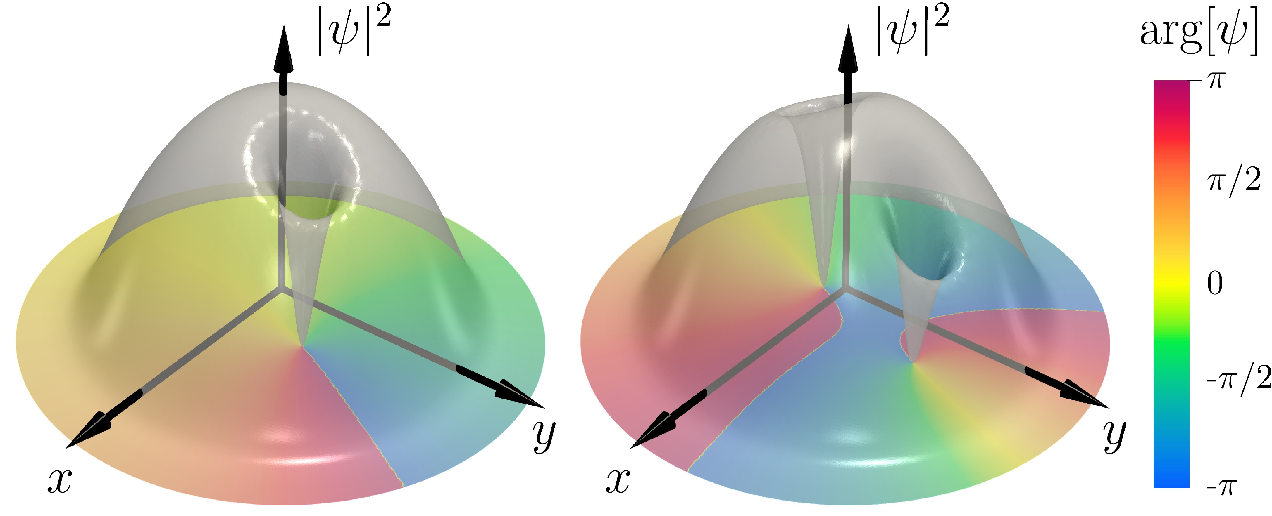
Figure 1: Examples of asymmetric vortex configurations of a Bose-Einstein condensate in an axially symmetric harmonic trap. The elevation of the semitransparent surface stems for the condensate density $|\psi|^{2}$, while the coloring projected onto the $xy$-plane indicates the value of the phase $\arg[\psi]$ of the macroscopic wave function. The examples shown are minima of the two dimensional Gross-Pitaevskii free energy (2), with non-integer values of the angular momentum (3) $L_{z}=0.80$ (left panel) and $L_{z}=1.48$ (right panel). The vortices precess around the trap center in accordance with the time dependent Gross-Pitaevskii equation (1).

Quantum vortices are the principal topological excitations in a cold atom Bose-Einstein condensate Matthews-1999 ; Chevy-2000 ; Raman-2001 ; Abo-Shaeer-2001 . A vortex is characterized by an integer valued circulation of the macroscopic wave function $\psi(\mathbf{x})$

$$\frac{1}{2\pi}\oint d{\boldsymbol{\ell}}\!\cdot\!{\boldsymbol{\nabla}}\arg[\psi]\in\mathbb{Z}$$

around its core. The time-dependent Gross-Pitaevskii equation Gross-1961 ; Pitaevskii-1961 governs the dynamics of the macroscopic wave function, at the level of the mean field theory. This is a nonlinear Schrödinger equation with a quartic nonlinearity that accounts for interactions between the atoms Pitaevskii-2003 ; Lieb-2006 ; Pethick-2008 ; Fetter-2009 ; Bao-2013 .

Vortices that appear in rotating cold atom Bose-Einstein condensates have been extensively studied, both experimentally and theoretically Haljan-2001 ; Fetter-2001 ; Fetter-2009 . At the level of the Gross-Pitaevskii equation these vortices are commonly modelled as stationary solutions in a co-rotating frame Butts-1999 ; Aftalion-2001 ; Seiringer-2002 ; Pitaevskii-2003 ; Lieb-2006 ; Pethick-2008 ; Fetter-2009 ; Bao-2013 . The rotating condensate accommodates growing angular velocity by forming vortices. This goes with a discontinuous increase in angular momentum: A rotating condensate does not support an arbitrary value of the angular momentum Butts-1999 .

Here we are interested in solutions of the Gross-Pitaevskii equation in a trapped condensate that does not rotate. In that case, the equation has no time independent solutions besides the trivial one $\psi(\mathbf{x})\equiv 0$. However, we show that whenever the non-rotating condensate supports a non-vanishing arbitrary valued angular momentum, there is a stable minimum energy solution of the time dependent Gross-Pitaevskii equation. These solutions describe eccentric vortices that precess around the center of the non-rotating axially symmetric trap, as illustrated in Fig. 1. In particular, the single vortex solutions are very similar to the experimentally observed precessing vortices reported in Anderson-2000 .

It is notable that even though the solutions that we present are minima of the ensuing free energy, they are not critical points of the free energy. Thus we employ methods of constrained optimization Fletcher-1987 ; Nocedal-1999 , to solve the time dependent Gross-Pitaevskii equation.

We note that the microscopic, individual atom angular momentum is certainly quantized. But as pointed out in Mottelson-1999 ; Kavoulakis-2000 (see also Butts-1999 ), in the limit where the number of atoms is very large, the condensate can accommodate arbitrary values of the macroscopic angular momentum that appears as a Noether change in the Gross-Pitaevskii equation. It was pointed out in Mottelson-1999 ; Kavoulakis-2000 and confirmed by the variational analysis in Kavoulakis-2000 , in the case of a single vortex, that a solution with arbitrary angular momentum must in general be time dependent. Our results confirm this proposal.

We emphasize the following difference between our approach that considers a non-rotating trap and builds on the ideas of Mottelson-1999 ; Kavoulakis-2000 , and the more common approach that considers vortices in a rotating trap, in terms of a co-rotating frame Butts-1999 ; Aftalion-2001 ; Seiringer-2002 ; Pitaevskii-2003 ; Lieb-2006 ; Pethick-2008 ; Fetter-2009 ; Bao-2013 : In the rotating trap problem, the minimal energy state is controlled by the value of the angular velocity of the trap that appears as a free parameter in the stationary, time independent co-rotating Gross-Pitaevskii energy functional. The vortices appear as critical points of this energy functional, as solutions of the time independent Gross-Pitaevskii equation they minimize an unconstrained variational problem. In contrast, in our case we use the fact that the angular momentum is conserved, thus we fix its value. The vortices are then solutions to a constrained optimization problem and solve the time dependent Gross-Pitaevskii equation. The difference between these two problems is detailed in Appendix B.

Since the vortex configurations that we find are simultaneously both constrained minima of the Gross-Pitaevskii free energy, and time dependent solutions of the ensuing Hamilton’s equation, they bear a certain resemblance to the concept of a classical Hamiltonian time crystal Shapere-2012 ; Wilczek-2012 . Our approach is modelled on the general theory developed in Alekseev-2020 ; see also Dai-2020 .

We shall further observe that in the case of a symmetric pair of two identical vortices, the evolution of the minimal energy vortex states, at specified angular momentum, brings about an exchange of the vortices. The exchange of identical bodies in two dimensions have been studied extensively, as it can be used to identify anyons. Anyons are two-dimensional quasiparticles that are neither fermions nor bosons Leinaas-1977 ; Wilczek-1982 . The anyon statistics implies that the exchange of the position of two identical particles results in a change of their quantum mechanical phase which differs from 0 (the case of bosons) or $\pi$ (the case of fermions); for reviews on anyons see e.g. Iengo-1992 ; Lerda-1992 ). The anyons, that can play an important role for quantum computing Kitaev-2003 , have recently been observed by electronic interferometry in quantum Hall effect experiments Nakamura-2020 .

2 Theoretical developments

We consider a two dimensional single-component Bose-Einstein condensate on the $xy$-plane with an axially symmetric, non-rotating, harmonic trap. This approximates for example an anisotropic three dimensional trap, resulting in an oblate condensate. Following Lieb-2002 ; Lieb-2006 we assume that the condensate describes a dilute limit of a large number of atoms, with a two-body repulsive interaction potential between the atoms. The condensate is described by a macroscopic wave function $\psi(\mathbf{x},t)$ whose dynamics obeys the (dimensionless) time dependent Gross-Pitaevskii equation Lieb-2002 ; Lieb-2006 :

$$i\partial_{t}\psi=-\frac{1}{2}\nabla^{2}\psi+\frac{|\mathbf{x}|^{2}}{2}\psi+g|\psi|^{2}\psi\equiv\ \frac{\delta F}{\delta\psi^{\star}}\,.$$ (1)

Here $g$ is a dimensionless coupling that accounts for the interactions between the atoms. In a typical Bose-Einstein condensate there are $N_{a}\sim 10^{4}-10^{6}$ ultracold alkali atoms and the corresponding coupling is typically $g\sim 1$–$10^{4}$; for discussion of the nondimensionalization, see, e.g, Bao-2013 and the Appendix A. The free energy $F$ in eq. (1) is

$$F=\int d^{2}x\left\{\frac{1}{2}|{\boldsymbol{\nabla}}\psi|^{2}+\frac{|\mathbf{x}|^{2}}{2}|\psi|^{2}+\frac{g}{2}|\psi|^{4}\right\}\,.$$ (2)

We observe that $F$ is a strictly convex functional, it can not have any critical points besides the global minimum $\psi\equiv 0$. Thus there are no nontrivial time independent solutions of the Gross-Pitaevskii equation (1), only time dependent nontrivial solutions of (1) can exist. Provided appropriate conditions can be introduced, these solutions can also minimize the free energy $F$ in the framework of constrained optimization. Thus, we search for time dependent solutions of (1) that are also minima of the free energy (2), where the latter is subject to an appropriate condition.

Indeed, besides the free energy (2) the time evolution equation (1) supports two additional conserved quantities, as Noether charges: The macroscopic angular momentum along the $z$-axis

$$L_{z}\ \equiv\ \int d^{2}x\,\psi^{\star}\,{\boldsymbol{e}}_{z}\cdot(-i\hbar\,\mathbf{x}\wedge{\boldsymbol{\nabla}})\psi\,$$ (3)

and the norm of the macroscopic wave function a.k.a. the number of particles

$$N\ \equiv\ \int d^{2}x\,\psi^{\star}\psi\,.$$ (4)

Accordingly, we search for solutions of the time dependent Gross-Pitaevskii equation (1), with fixed values of both the angular momentum $L_{z}$ and the number of particles; in the following, with no loss of generality, we normalize the wave function so that $N=1$ (see Appendix A for details). On the other hand, the angular momentum (3), can assume arbitrary values $L_{z}=l_{z}$, and even in the case of a single vortex the values $l_{z}$ of the angular momentum are not expected to be integer valued Mottelson-1999 ; Kavoulakis-2000 .

The Lagrange multiplier theorem Marsden-1999 states that with fixed angular momentum (3) and fixed number of particles (4), the minimum of $F$ is also a critical point of

$$F_{\lambda}=F+\lambda_{z}(L_{z}-l_{z})+\lambda_{N}(N-1)\,.$$ (5)

Here $\lambda_{z}$, $\lambda_{N}$ are the Lagrange multipliers that enforce the values $L_{z}=l_{z}$ and $N=1$, respectively. The critical points ($\psi_{cr},\lambda_{z}^{cr},\lambda_{N}^{cr}$) of $F_{\lambda}$ (5) obey

$$-\frac{1}{2}\nabla^{2}\psi +\frac{|\mathbf{x}|^{2}}{2}\psi+g|\psi|^{2}\psi=-\lambda_{N}\psi+i\lambda_{z}{\boldsymbol{e}}_{z}\cdot\mathbf{x}\wedge{\boldsymbol{\nabla}}\psi\,$$

$$~{}\text{together with}~{}~{}L_{z}=l_{z}\,~{}~{}\text{and}\,~{}N=1\,.$$ (6)

Let $\psi_{min}(\mathbf{x})$ be a solution of (6) that is also a minimum of (2), and let $\lambda^{min}_{N}$ and $\lambda^{min}_{z}$ denote the corresponding solutions for the Lagrange multipliers. Whenever the solutions for the Lagrange multipliers do not vanish, $\psi_{min}(\mathbf{x})$ cannot be a critical point of the free energy $F$ in (2). Instead, it generates a time dependent solution $\psi(\mathbf{x},t)$ of (1) which, from (6), with the initial condition $\psi(\mathbf{x},t=0)=\psi_{min}(\mathbf{x})$ obeys the linear time evolution

$$i\partial_{t}\psi=-\lambda^{min}_{N}\psi+i\lambda^{min}_{z}{\boldsymbol{e}}_{z}\cdot\mathbf{x}\wedge{\boldsymbol{\nabla}}\psi\,,$$ (7)

where both $\lambda^{min}_{N}$ and $\lambda^{min}_{z}$ are time independent Alekseev-2020 .

Whenever either of the Lagrange multipliers is non-vanishing, the minimum energy solution is time dependent. But the time evolution amounts to a simple phase multiplication only when $\psi_{min}(\mathbf{x})$ is an eigenstate of the angular momentum operator; below we show that this can only occur for $l_{z}=1$, for all other values of $l_{z}\neq 0$ the minimum energy solution always describes a precessing vortex configuration.

The minimum energy wave function $\psi_{min}(\mathbf{x})$ spontaneously breaks both Noether symmetries. The time evolution equation (7) describes a symmetry transformation of $\psi_{min}(\mathbf{x})$, that is generated by a definite linear combination of the two conserved Noether charges:

$$i\partial_{t}\psi=-\lambda^{min}_{N}\frac{\delta N}{\delta\psi^{\star}}-\lambda^{min}_{z}\frac{\delta L_{z}}{\delta\psi^{\star}}\equiv\ -\lambda^{min}_{N}\{N,\psi\}-\lambda^{min}_{z}\{L_{z},\psi\}\,,$$ (8)

where $\{\ ,\ \}$ is the Poisson bracket. This is an example of spontaneous symmetry breaking, but now the symmetry breaking minimum energy configuration is time dependent Alekseev-2020 .

3 Numerical simulations

To search for minimum energy solutions of the time dependent Gross-Pitaevskii equation, we numerically minimize the free energy (2) subject to the conditions $L_{z}=l_{z}$ and $N=1$. The problem is discretized within a finite-element framework Hecht-2012 , and the constrained optimization problem is then solved using the Augmented Lagrangian Method (see details of the numerical methods in Appendix C). Minimal energy states for angular momentum values $l_{z}\in(0,2]$ with $N=1$, and for three representative values of the interaction coupling $g=5$, $g=100$ and $g=400$ are displayed in figure 2; see also additional animations in Supplementary materials supp .

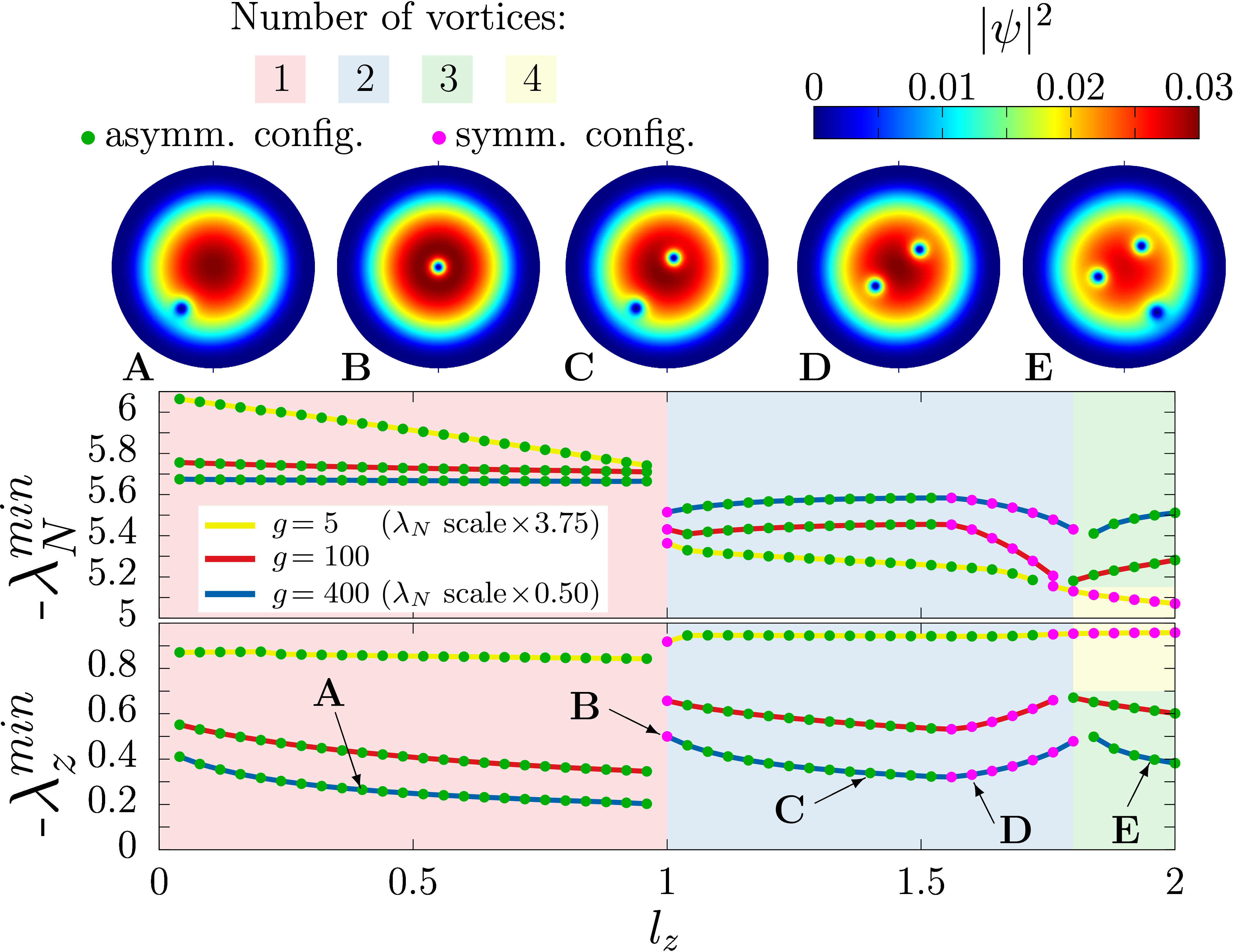
Figure 2: Minimum energy states for angular momenta $l_{z}\in(0,2]$. The bottom row shows the dependence of the multipliers $\lambda^{min}_{N}$ and $\lambda^{min}_{z}$ on the angular momentum $l_{z}$ for $g=5$, $100$ and $400$. The panels on the top row display the density of the condensate $|\psi|^{2}$ for qualitatively different solutions with $g=400$, obtained for different values of $l_{z}$ (zoomed to relevant data while the actual numerical domain is larger). At the vortex core the density $|\psi|^{2}$ vanishes and the phase circulation is $2\pi$. The five regimes A – E are detailed in the text.

For non-vanishing values of the angular momentum $0<l_{z}<1$ the minimum energy configuration $\psi_{min}(\mathbf{x})$ is an eccentric vortex that precesses around the trap center (see regime A). As $l_{z}$ increases the vortex core approaches the trap center. This kind of eccentric precessing vortices have been previously proposed theoretically in Kavoulakis-2000 . They appear very similar to the precessing vortices that have been observed experimentally Anderson-2000 .

As shown in regime B, when $l_{z}=1$, the core position coincides with the center of the trap, and the Lagrange multipliers feature a discontinuity. At this value of $l_{z}$, our solution coincides with the single vortex solution that has been described extensively in the literature Pethick-2008 ; Pitaevskii-2003 ; Lieb-2006 ; Fetter-2009 ; Bao-2013 ; Aftalion-2001 ; Seiringer-2002 . When $l_{z}$ becomes larger than one, a second vortex appears, and there are two qualitatively different two-vortex configurations. As $l_{z}$ increases, these are sequentially asymmetric (regime C) and then symmetric (regime D) with respect to the trap center. Because it depends on $g$, there is no universal value of $l_{z}$ that separates these two regimes. At higher values of angular momentum, $l_{z}\approx 1.8$ with the exact value depending on $g$, additional vortices start entering the condensate; this is the regime E in figure 2. Remark that for $g=100$ and $g=400$ a third vortex moves towards the trap center as $l_{z}$ increases, while for $g=5$ a pair of vortices enters. Further increase of the angular momentum introduces additional vortices in the condensate (not shown).

The case $l_{z}=1$, labelled by B in figure 2, is a special case. There, the core of the vortex coincides with the center of the trap. The corresponding $\psi_{min}(\mathbf{x})$ is an angular momentum eigenstate with eigenvalue $l_{z}=1$, and the solution of the time dependent Gross-Pitaevskii equation (7) is merely an overall phase rotation with no change in the core position. However, for generic $l_{z}$ the minimum energy configuration $\psi_{min}(\mathbf{x})$ is not an eigenstate of the angular momentum.

We have simulated the time evolution (1) of the minimum energy configuration $\psi_{min}(\mathbf{x})$ using a Crank-Nicolson algorithm. Simulation details together with animations of the time evolution can be found in the Appendix C. For all values of $l_{z}\neq 1$ the vortex configuration precesses uniformly around the trap center. This uniform rotation is a consequence of the equation (7) which determines the time evolution of the minimal energy configurations, in terms of the two conserved charges.

4 Exchange of vortices

Finally, an interesting phenomenon occurs for the time evolution of a symmetric pair of identical vortices (corresponding to the regime D of figure 2). The time evolution of such a vortex pair, with $g=5$, is displayed in figure 3. The vortex pair rigidly rotates around the trap center at a constant distance, with an angular velocity specified by $\lambda^{min}_{z}\equiv-\Omega$. In addition the phase of the wave function evolves with a rate that depends on $\lambda^{min}_{N}$. This coincides with the rate of change in the phase $\arg[\psi](t)$, measured at the center of the trap. Similarly, the rate of change of $\theta(t)$ that measures the rotation of the pair, equals $\lambda^{min}_{z}$ . Since the two Lagrange multipliers are in general not commensurate, it follows that when the time evolution exchanges the position of two identical vortices, the change in the phase of the wave function is not by an integer multiple of $\pi$.

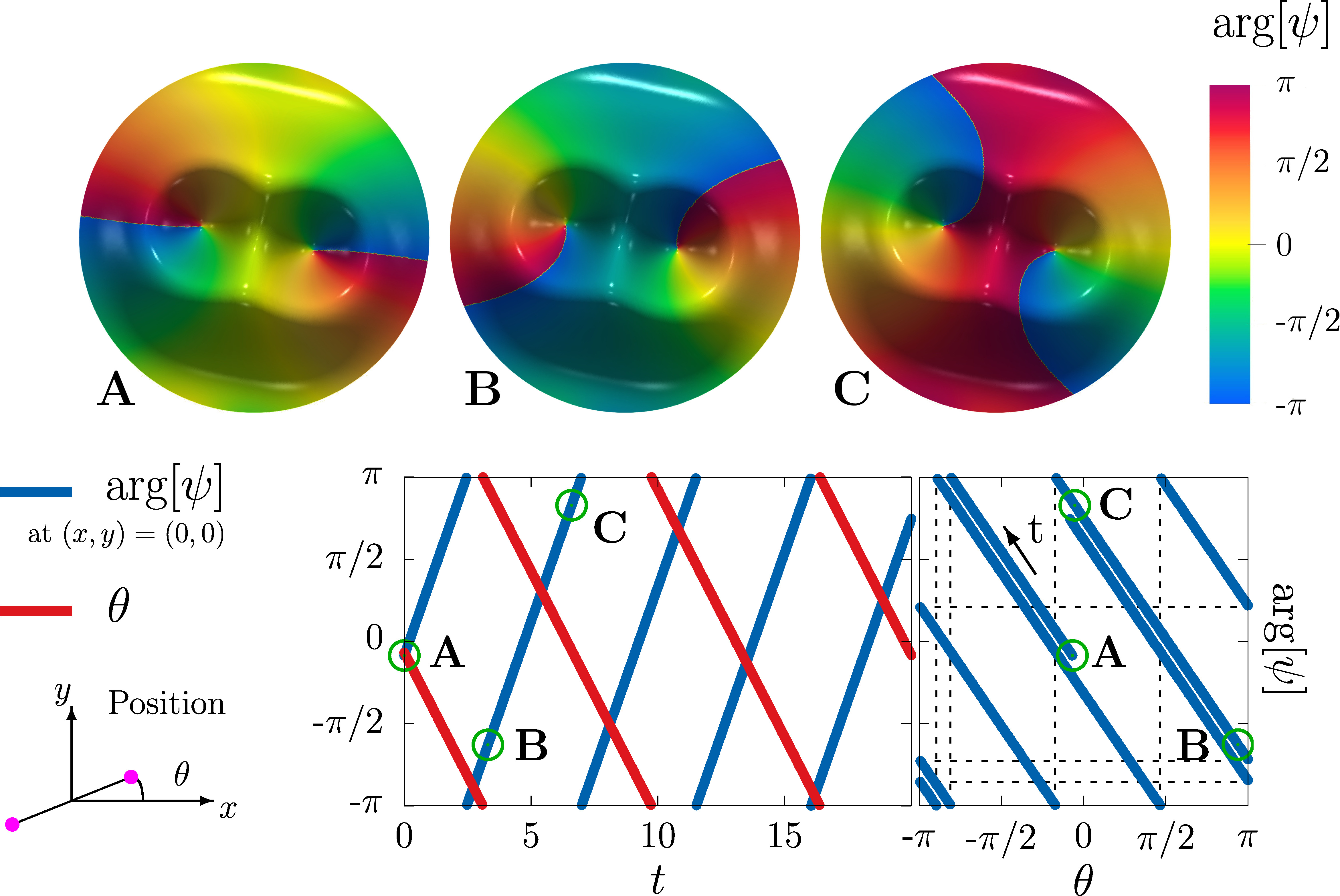
Figure 3: The evolution of a minimum energy configuration $\psi_{min}(\mathbf{x})$, in the case of a symmetric vortex pair (with $g=5$) in region D of figure 2. The bottom panels show the evolution of $\theta$, the rotation angle of the pair, and of the value of the phase $\arg[\psi]$ measured at the center of the trap. The three panels A–C on the top row are snapshots displaying the phase $\arg[\psi]$ after rotations $\theta=\theta_{0}$, $\theta=\theta_{0}+\pi$ and $\theta=\theta_{0}+2\pi$ respectively. Since the Lagrange multipliers $\lambda_{N}^{min}$ and $\lambda_{z}^{min}$ are not commensurate, $\arg[\psi](t)$ and $\theta(t)$ feature different periodicities. As a result after $\pi$ rotations of the pair the phase profile is not simply an overall phase multiplication.

The quantum mechanical exchange of two identical bodies, with ensuing phase change, is familiar from description of anyons Leinaas-1977 ; Wilczek-1982a ; Wilczek-1982 . The similarity to that scenario can be elaborated further, by following Wilczek-1982a to rewrite the time evolution (7) as follows:

$$i\partial_{t}\psi=\Omega\,\mathbf{L}^{cov}_{z}\psi\ \equiv\ \Omega({\boldsymbol{e}}_{z}\cdot\mathbf{L}+\phi\,{\boldsymbol{e}}_{z}\cdot\mathbf{x}\wedge{\mathbf{A}})\psi\,.$$ (9)

Here $\mathbf{L}=-i\mathbf{x}\wedge{\boldsymbol{\nabla}}$ is the canonical angular momentum, the parameter $\phi=\lambda^{min}_{N}/\lambda^{min}_{z}$, and the flux of ${\mathbf{A}}={\boldsymbol{\nabla}}\tan^{-1}x/y$ equals $2\pi$ around any counter-clockwise path that encircles the $z$-axis once. Notably, in the case of two identical vortices $\mathbf{x}$ coincides with their relative coordinate in a center-of-mass frame. Furthermore, the equation (9) is akin a time dependent linear Schrödinger equation that describes the evolution of a charged point particle, moving on the ($x,y$) plane under the influence of a unit strength magnetic vortex filament along the $z$-axis. The corresponding Hamiltonian comprises the $z$-component of the covariant angular momentum $\mathbf{L}^{cov}_{z}$. We note that when $\phi\not=0$, the rotations around $z$-axis, i.e. the changes in the polar angle $\theta$, are generated by the covariant angular momentum.

To find the solutions of (9) we first remove ${\mathbf{A}}$ by phase multiplication, and then proceed with separation of variables in terms of polar coordinates ($r,\theta$).

$$\psi(\mathbf{x},t)\ =\ e^{-iEt}\mathcal{X}(r,\theta)\,e^{-i\phi\!\int\limits_{\mathbf{x}_{0}}^{\mathbf{x}}{\mathbf{A}}\cdot d\boldsymbol{\ell}}\,,$$ (10)

The single valuedness of the wave function $\psi(\mathbf{x},t)$ implies that $\mathcal{X}(r,\theta)$ is generally not single valued as it obeys

$$\mathbf{L}_{z}\mathcal{X}_{n}=(n+\phi)\mathcal{X}_{n}\,.$$ (11)

The solution of the time evolution (9) is thus

$$\psi(\mathbf{x},t)=e^{-i\phi\!\int\limits_{\mathbf{x}_{0}}^{\mathbf{x}}{\mathbf{A}}\cdot d\boldsymbol{\ell}}\sum_{n}f_{n}(r)e^{-i(n+\phi)(\Omega t-\theta)}\,.$$ (12)

Here the $f_{n}(r)$ form an orthogonal set of normalizable, real valued functions, they are selected so that (12) describes the energy minimizer $\psi_{min}(\mathbf{x})$ of (6), (1) at $t=0$.

5 Summary and outlook

In summary, we have investigated the time dependent two-dimensional Gross-Pitaevskii equation, that models dynamics in an axially symmetric harmonic trap. The equation supports two Noether charges that correspond to the number of atoms and to the axial component of the macroscopic angular momentum, respectively. We have used the methodology of constrained optimization to construct solutions that minimize the Gross-Pitaevskii free energy, with a fixed number of atoms and as function of the macroscopic angular momentum to which we have assigned arbitrary numerical values. For generic angular momentum values, a minimum energy configuration always exists and it describes eccentric vortices that precess uniformly around the center of the trap. In particular, no time independent solution can exist in a non-rotating cylindrically symmetric trap. Moreover, whenever the solution describes two identical vortices, the time evolution exchanges their positions but the phase of their common wave function evolves in a nontrivial fashion.

We foresee that the vortex precession in a non-rotating condensate that we have described, can be realized and observed in a variety of laboratory experiments; the precessing vortices already reported in Anderson-2000 appear to be very similar to the vortex precession that we have simulated. There are several conceivable experimental setups, where vortices can form in a non-rotating condensate. These include vortex formation by optical photon beams that carry a non-vanishing angular momentum, with appropriate topologies Marzlin-1997 ; Bolda-1998 ; Dum-1998 ; Leanhardt-2002 . Additional experimental set-ups can be built on thermal quenching in combination with the Kibble-Zurek mechanism Kibble-1976 ; Zurek-1985 ; Zurek-1996 ; Anglin-1999 . This mechanism describes how topological defects form during rapid symmetry breaking transitions. There are already several laboratory examples that are relevant to the scenario we have studied, including neutron irradiation in the case of superfluid ³He Ruutu-1996 ; Eltsov-2000 , evaporative cooling in the case of ultracold ${}^{8}7$Rb atoms Weiler-2008 ; Freilich-2010 .

Appendices

Appendix A Nondimensionalization of the Gross-Pitaevskii equation

In the main body of the paper, the dynamics of a Bose-Einstein ultracold atoms is described by the dimensionless Gross-Pitaevskii equation. Here, we derive this dimensionless form from the original equation (see e.g. Bao-2013 ). In the ultracold dilute regime, the Bose-Einstein condensate state of $N_{a}$ identical atoms is described by the macroscopic wave function $\Psi$, whose dynamics obey

$$i\hbar\partial_{t}\Psi =\left[-\frac{\hbar^{2}}{2m}\nabla^{2}+V(\mathbf{x})+\frac{N_{a}}{N}g_{0}|\Psi|^{2}\right]\Psi\,,$$ (13a)

where $$N=\int|\Psi|^{2}\,,~{}~{}\text{and}~{}~{}g_{0}=\frac{4\pi\hbar^{2}a_{s}}{m}\,.$$ (13b)

Here, $\nabla^{2}\equiv{\boldsymbol{\nabla}}\!\cdot\!{\boldsymbol{\nabla}}$ is the Laplace operator, $m$ is the mass of the atoms, $\hbar$ is the reduced Planck’s constant, and $a_{s}$ is $s$-wave scattering length of the atoms. Note that for practical purposes, we introduce $N$ to be the norm of the condensate, while $N_{a}$ is the actual number of atoms in the condensate. The harmonic oscillator trap potential reads as

$$V(\mathbf{x})=\frac{m}{2}\big{(}\omega^{2}_{x}x^{2}+\omega^{2}_{y}y^{2}+\omega^{2}_{z}z^{2}\big{)}\,,$$ (14)

where $\omega_{x}\leq\omega_{y}\leq\omega_{z}$ are the trapping frequencies in the different spatial directions. The dimensionless units are obtained by the following rescaling

$$t=t_{s}\tilde{t}\,,~{}~{}\mathbf{x}=x_{s}\tilde{x}\,,~{}~{}\Psi=x_{s}^{-3/2}\psi\,,~{}~{}\text{where}~{}~{}t_{s}=\frac{1}{\omega_{x}}\,,~{}~{}\text{and}~{}~{}x_{s}=\sqrt{\frac{\hbar}{m\omega_{x}}}\,.$$ (15)

Hence, after dropping the $\tilde{\,}$, the dimensionless Gross-Pitaevskii equation is

$$i\partial_{t}\psi =\left[-\frac{1}{2}\nabla^{2}+V(\mathbf{x})+g|\psi|^{2}\right]\psi\,,$$ (16a)

$$~{}\text{where}~{}~{}V(\mathbf{x})=\frac{1}{2}\sum_{\alpha=x,y,z} \left(\frac{\omega_{\alpha}}{\omega_{x}}\right)^{2}x^{2}_{\alpha}\,,~{}N=\!\int|\psi|^{2}\,,~{}\text{and}~{}~{}g=\frac{4\pi a_{s}N_{a}}{x_{s}N}\,.$$ (16b)

The dimensionless time dependent Gross-Pitaevskii equation (16), is obtained for a three dimensional harmonic trap. In the main body of the paper, we consider the case of a two Bose-Einstein condensate. The two dimensional problem fairly approximates a disk-shaped condensate with small height in $z$-direction, for the trap frequencies $\omega_{x}\approx\omega_{y}$ and $\omega_{z}\gg\omega_{x}$. This results in a further rescaling of the coupling constant $g_{2d}=g_{3d}\sqrt{\frac{\omega_{z}}{2\pi\omega_{x}}}$. For detailed derivation see, e.g., Bao-2013 .

The dimensionless coupling $g$ is thus the parameter of the accounts for the interactions between atoms. In the numerical investigations we choose values $g$ that are representative of a Bose-Einstein condensate of ultracold alkali atoms. The Table 1 shows typical experimental values of trapped ultracold atoms, and the corresponding estimates for the length scales and the dimensionless coupling $g$.

Atoms	$m\ (kg)$	$a_{s}\ (m)$	$\omega_{x}\ (rad.s^{-1})$	$N_{a}$
${}^{87}Rb$ Anderson-1995	$1.44\times 10^{-25}$	$5.1\times 10^{-9}$	20	$10^{2}\sim 10^{7}$
${}^{23}Na$ Davis-1995	$3.817\times 10^{-26}$	$2.75\times 10^{-9}$	$2\pi\times 200$	$\times 10^{4}\sim 5\times 10^{5}$

Atoms	$x_{s}\ (m)$	$\frac{4\pi a_{s}}{x_{s}}$	$g\ (\times N=1)$
${}^{87}Rb$ Anderson-1995	$6.0\times 10^{-6}$	$1.1\times 10^{-2}$	$1\sim 10^{5}$
${}^{23}Na$ Davis-1995	$1.5\times 10^{-6}$	$2.3\times 10^{-2}$	$10^{2}\sim 10^{4}$

Table 1: Typical physical values for various atomic Bose-Einstein condensates, and the resulting scale and dimensionless coupling. The reduced Planck constant is $\hbar=1.05\times 10^{-34}J.s$.

Appendix B Constrained minimization with fixed angular momentum
versus minimization at constant angular velocity

In the main body of the paper, we emphasize that there is a difference between the common set-up that describes vortices in a rotating trap in terms of a free energy expressed in the co-rotating frame Butts-1999 ; Aftalion-2001 ; Seiringer-2002 ; Pitaevskii-2003 ; Lieb-2006 ; Pethick-2008 ; Fetter-2009 ; Bao-2013 , and the present set-up where vortices occur in a non-rotating trap; the present set-up was first addressed in Mottelson-1999 ; Kavoulakis-2000 . Here we clarify the difference, by a direct comparison of the two cases:

In the case of a rotating trap, vortices are created by rotating the trap, with a constant angular velocity $\Omega$. The free energy $F^{\Omega}$ is expressed in the co-rotating frame, and the vortices are the critical points of the free energy. The vortex structures can then be investigated as a function of the externally applied angular velocity $\Omega$. In contrast, in our case the trap does not rotate. Instead, we use the fact that the angular momentum $L_{z}$ of the condensate is a conserved quantity, and the condensate carries a corresponding angular momentum value $L_{z}=l_{z}$. The ensuing minimal free energy configuration is a solution of a constrained optimization problem that minimizes the free energy $F$, subject to the condition $L_{z}=l_{z}$. The two free energies are related as follows:

$$F^{\Omega}=F-\Omega L_{z}\,,~{}~{}~{}~{}\text{where}~{}~{}L_{z}\ \equiv\ \int d^{2}x\,\psi^{\star}\,{\boldsymbol{e}}_{z}\cdot(-i\hbar\,\mathbf{x}\wedge{\boldsymbol{\nabla}})\psi\,.$$ (17)

Due to the constraint, the free energy minimizer is in general not a critical point of $F$. But it can be located using the Lagrange multiplier theorem Marsden-1999 , in the framework of constrained optimization Fletcher-1987 ; Nocedal-1999 . Whenever the minimizer of the free energy $F$ is not a critical point, it describes a solution of a time dependent Gross-Pitaevskii equation.

In addition, in both cases the norm of the condensate wave function (i.e. the particle number) needs to be accounted for. Here the goal is to clarify the difference between the rotating and non-rotating cases. Therefore, in our comparison we treat the constraint $N=1$ the same way, both when searching for the minimum of $F^{\Omega}$ and $F$, by using the Lagrange multiplier theorem. For the problem we consider, the Lagrange multiplier theorem Marsden-1999 states that with fixed angular momentum and fixed number of particles $N$, the minimum of $F$ is also a critical point of

$$F_{\lambda}\equiv F+\lambda_{z}(L_{z}-l_{z})+\lambda_{N}(N-1)\,.$$ (18)

Here $\lambda_{z}$, $\lambda_{N}$ are the Lagrange multipliers that enforce the values $L_{z}=l_{z}$ and $N=1$ respectively. On the other hand, for a rotating condensate, the minimum of $F^{\Omega}$ is a critical point of the following free energy

$$F_{\lambda}^{\Omega}\equiv F^{\Omega}+\lambda_{N}(N-1)=F+\Omega L_{z}+\lambda_{N}(N-1)\,,$$ (19)

where $\lambda_{N}$ is the (only) Lagrange multiplier that enforces $N=1$. Note that the present Lagrange multiplier $\lambda_{N}$ is commonly treated as a chemical potential that is an externally controlled parameter, in par with $\Omega$. This is not the case here, as $\lambda_{N}$ has to be adjusted to satisfy the constraint. The critical points of $F_{\lambda}$ and $F_{\lambda}^{\Omega}$ obey respectively

$$F_{\lambda}:~{}~{}-\frac{1}{2}\nabla^{2}\psi +\frac{|\mathbf{x}|^{2}}{2}\psi+g|\psi|^{2}\psi=-\lambda_{N}\psi+i\lambda_{z}{\boldsymbol{e}}_{z}\cdot\mathbf{x}\wedge{\boldsymbol{\nabla}}\psi\,,$$ (20a)

$$\text{and the conditions}~{}L_{z}=l_{z}~{}\text{and}~{}N=1\,,$$

$$F_{\lambda}^{\Omega}:~{}~{}-\frac{1}{2}\nabla^{2}\psi +\frac{|\mathbf{x}|^{2}}{2}\psi+g|\psi|^{2}\psi-i\Omega\,\,{\boldsymbol{e}}_{z}\cdot\mathbf{x}\wedge{\boldsymbol{\nabla}}\psi=-\lambda_{N}\psi\,,$$ (20b)

$$\text{and the condition}~{}N=1\,.$$

Note that in a numerical simulation $\Omega$ is an input parameter that is fixed during the simulation, while $\lambda_{z}$ is adjusted sequentially, to satisfy the constraint (according to the Augmented Lagrangian Method, see details in Sec. C.2). The differences between the two approaches are summarized at the end of this section in Table 2.

Critical	Obey the equation	Satisfy	Control	Mult.	Output
pts. of	Obey the equation		params.
$F_{\lambda}$	$-\frac{1}{2}\nabla^{2}\psi+\frac{|\mathbf{x}|^{2}}{2}\psi+g|\psi|^{2}\psi=$	$L_{z}\!={\color[rgb]{1,0,0}{l_{z}}}$	$g$, ${\color[rgb]{1,0,0}{l_{z}}}$	${\color[rgb]{0.5,0.0,1.0}{\lambda_{N}}}$,	${\color[rgb]{0.5,0.5,0.0}{\lambda_{N}^{min}}}$, ${\color[rgb]{0.5,0.5,0.0}{\lambda_{z}^{min}}}$
	$-{\color[rgb]{0.5,0.0,1.0}{\lambda_{N}}}\psi+i{\color[rgb]{0.5,0.0,1.0}{\lambda_{z}}}\,\,{\boldsymbol{e}}_{z}\cdot\mathbf{x}\wedge{\boldsymbol{\nabla}}\psi$	and $N=1$		${\color[rgb]{0.5,0.0,1.0}{\lambda_{z}}}$	${\color[rgb]{0.5,0.5,0.0}{\psi_{min}}}$
$F_{\lambda}^{\Omega}$	$-\frac{1}{2}\nabla^{2}\psi+\frac{|\mathbf{x}|^{2}}{2}\psi+g|\psi|^{2}\psi$	$N=1$	$g$, ${\color[rgb]{1,0,0}{\Omega}}$	${\color[rgb]{0.5,0.0,1.0}{\lambda_{N}}}$	${\color[rgb]{0.5,0.5,0.0}{\lambda_{N}^{min}}}$,
	$-i{\color[rgb]{1,0,0}{\Omega}}\,\,{\boldsymbol{e}}_{z}\cdot\mathbf{x}\wedge{\boldsymbol{\nabla}}\psi=-{\color[rgb]{0.5,0.0,1.0}{\lambda_{N}}}\psi$				${\color[rgb]{0.5,0.5,0.0}{\psi_{min}}}$

Table 2: Summary of the differences: The red font shows the parameters that are given as input to the corresponding minimization problem. The purple font highlights the Lagrange multipliers. In a numerical simulation, these are sequentially adjusted according the Augmented Lagrangian Algorithm, until the constraints are satisfied (and the minima of $F_{\lambda}$ are found). The olive color fonts show the output quantities obtained in the numerical simulations.

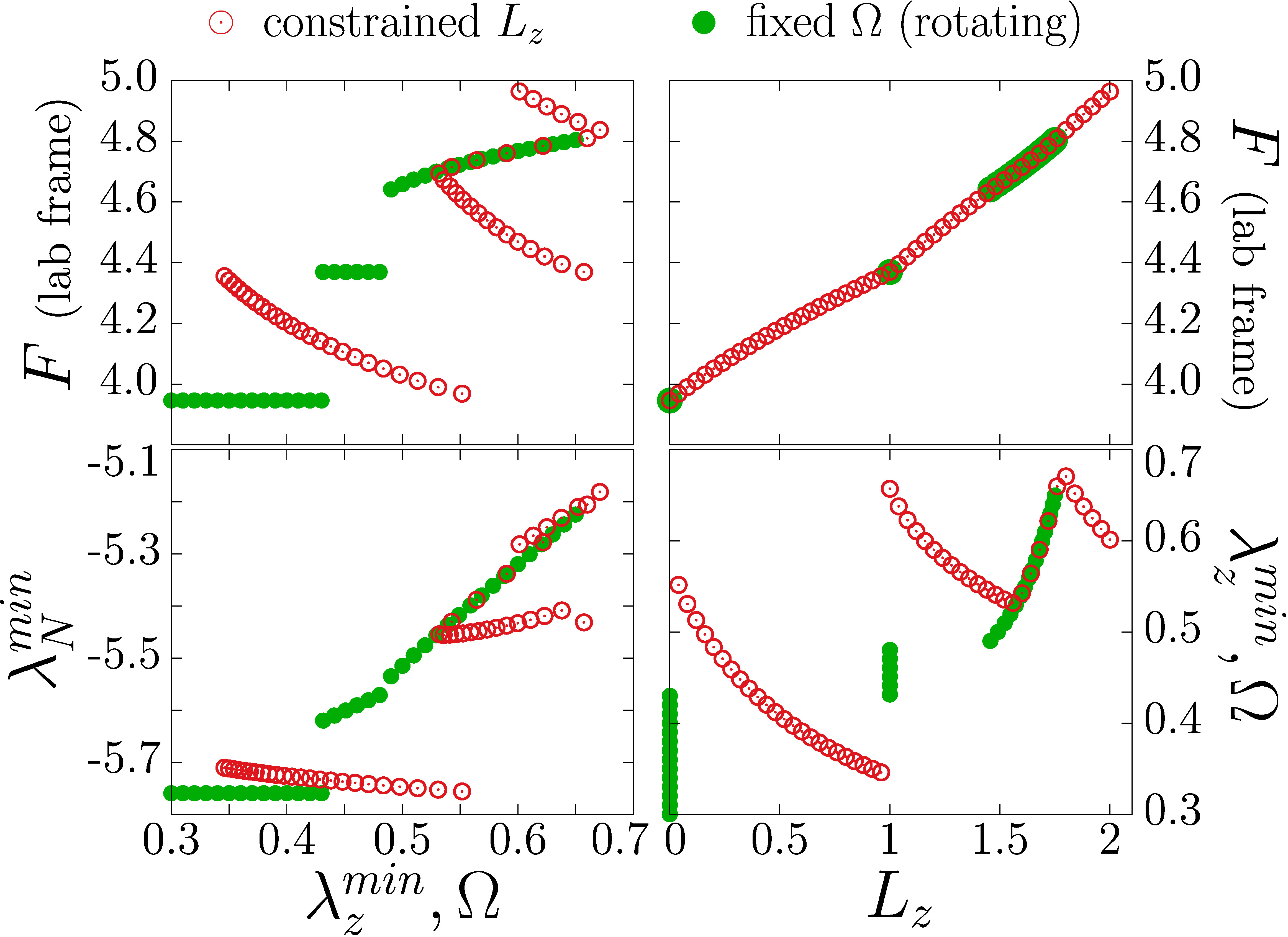
Figure 4: Detailed comparison of the solutions to the two equations (20) for $g=100$. The panels on the top row display the energy, in a non-rotating frame, as a function of angular velocity $\Omega$ (left) and value of angular momentum $L_{z}$ (right). The empty (red) circles denote the results from the constrained minimization at given value of the angular momentum $L_{z}$. The filled (green) circles show the results from the minimization of a rotated condensate at given angular velocity $\Omega$.

Comparison of the minimal energy solutions of the two equations (20), can be seen in figure 4. The results are indeed quite different. In particular, the free energy (evaluated in a non-rotating laboratory frame) that is displayed on the panels on the top row of figure 4, show that the minimization with fixed angular frequency $\Omega$ cannot support solutions with arbitrary values of angular momentum. Indeed, there are excluded ranges

$$L_{z}\in[0,1[~{}\cup~{}]1,1.457[~{}\cup~{}]1.75,2.68[\cdots\,,$$ (21)

where there are no rotation-induced stable vortex states (see the green dots on the top right panel). This is in agreement with the known results for rotating Bose-Einstein condensates; compare for example the green dots in the top left panel of figure 4, e.g. with the results shown in figure 2 of Butts-1999 . In contrast, in the present case, there cannot be any excluded values of the angular momentum in the equation (20a) (see the red dots on the top right panel). Those vortex configurations with angular momentum in the excluded ranges (21) describe eccentric asymmetric vortex configurations that precess around the trap center.

Observe that in the case of equation (20a), there is multi-valuedness in the free energy (red dots), as a function of the Lagrange multiplier $\lambda_{z}$; see for example the top left panel at $\lambda_{z}^{min}\approx 0.55$ which displays 3 different states at the same value of $\lambda_{z}$. These are a single eccentric vortex, an asymmetric vortex pair, and a symmetric vortex pair for increasing free energy, respectively. These configurations have both a different angular momentum value, and a different value of the Lagrange multiplier $\lambda_{N}^{min}$ (see the bottom panels) which plays the role of a chemical potential. The present comparisons, summarized in figure 4, show that the two equations (20a) and (20b) do indeed describe two quite different physical scenarios.

Appendix C Details of the numerical methods

In the numerical investigations in the main body of the paper, we use Finite-Element Methods (FEM) (see e.g. Hutton-2003 ; Reddy-2005 ) both for the minimization and for the time-evolution. In practice we use the finite-element framework provided by the FreeFEM library Hecht-2012 . Within the finite-element framework, the constrained minimization is addressed using an Augmented Lagrangian Method together within a non-linear conjugate gradient algorithm. The time-dependent Gross-Pitaevskii equation, is integrated using a Crank-Nicolson algorithm with a forward extrapolation of the nonlinear term.

C.1 Finite-element formulation

We consider the domain $\Omega$ which a bounded open subset of $\mathbb{R}^{2}$ and denote $\partial\Omega$ its boundary. $H(\Omega)$ stands for the Hilbert space, such that a function belonging to $H(\Omega)$, and its weak derivatives have a finite $L^{2}$-norm. Furthermore, $\mathcal{H}(\Omega)=\{u+iv\,|\,u,v\in H(\Omega)\}$ denotes the Hilbert spaces of complex-valued functions. The Hilbert spaces of real- and complex-valued functions are equipped with the inner products $\langle\cdot,\cdot\rangle$, defined as:

$$\left\langle u,v\right\rangle=\int_{\Omega}uv\,,~{}\text{for}~{}u,v\in H({\Omega})\,,~{}~{}~{}~{}\text{and}~{}~{}~{}~{}\left\langle u,v\right\rangle=\int_{\Omega}u^{\star}v\,,~{}\text{for}~{}u,v\in\mathcal{H}({\Omega})\,.$$ (22)

The spatial domain $\Omega$ is discretized as a mesh of triangles using for the Delaunay-Voronoi algorithm, and the regular partition $\mathcal{T}_{h}$ of $\Omega$ refers to the family of the triangles that compose the mesh. Given a spatial discretization, the functions are approximated to belong to a finite-element space whose properties correspond to the details of the Hilbert spaces to which the functions belong. We define ${P}^{(2)}_{h}$ as the $2$-nd order Lagrange finite-element subspace of $H(\Omega)$, and correspondingly $\mathcal{P}^{(2)}_{h}$ for $\mathcal{H}(\Omega)$. Now, the physical degrees of freedom can be discretized in their finite element subspaces. And we define the finite-element description of the degrees of freedom as $\psi\mapsto\psi^{(h)}\in\mathcal{P}^{(2)}_{h}$. This describes a linear vector space of finite dimension, for which a basis can be found. The canonical basis consists of the shape functions $\phi_{k}(\mathbf{x})$, and thus

$$V_{h}(\mathcal{T}_{h},\mathrm{P}^{(2)})=\Big{\{}w(\mathbf{x})=\sum_{k=1}^{M}w_{k}\phi_{k}(\mathbf{x}),\phi_{k}(\mathbf{x})\in\mathrm{P}^{(2)}_{h}\Big{\}}\,.$$ (23)

Here $M$ is the dimension of $V_{h}$ (the number of vertices), the $w_{k}$ are called the degrees of freedom of $w$ and M the number of the degrees of freedom. To summarize, a given function is approximated as its decomposition: $w(\mathbf{x})=\sum_{k=1}^{M}w_{k}\phi_{k}(\mathbf{x})$, on a given basis of shape functions $\phi_{k}(\mathbf{x})$ of the polynomial functions $\mathrm{P}^{(2)}$ for the triangle $T_{i_{k}}$. The finite element space $V_{h}(\mathcal{T}_{h},\mathrm{P}^{(2)})$ hence denotes the space of continuous, piecewise quadratic functions of $x$, $y$ on each triangle of $\mathcal{T}_{h}$.

C.2 Constrained minimization: Augmented Lagrangian Method

In the main body of the paper, we aim to minimize the free energy while enforcing a set of two conditions. Such problems, referred to as constrained optimization are studied in great details, see for example textbooks Gill-1981 ; Fletcher-1987 ; Nocedal-1999 ; Birgin-2008 . Here we describe the numerical algorithms that were used in the main body of the paper, to solve the constrained optimization problem. The Augmented Lagrangian Method (ALM) used to solve the constrained optimization is based on the following. In terms of the original energy functional to be minimized $F$, and the set of conditions $C_{i}$, the augmented Lagrangian $F^{\mathrm{aug}}$ is defined as

$$F^{\mathrm{aug}}:=F+\frac{\mu}{2}\left(\sum_{j}C_{j}^{2}\right)+\sum_{j}\lambda_{j}C_{j}\,.$$ (24)

Here $\mu$ is a penalty parameter and $\lambda_{j}$ are the Lagrange multipliers associated with the conditions $C_{j}$. In the Augmented Lagrangian Method, the augmented Lagrangian is minimized, and the penalty $\mu$ is iteratively increased while the multipliers $\lambda_{j}\leftarrow\lambda_{j}+\mu C_{j}$ until all conditions are satisfied with a specified accuracy. The ALM algorithm has the property to converge in a finite number of iterations. Our choice for the minimization algorithm within each ALM iteration is a non-linear conjugate gradient algorithm Hestenes-1952 ; Fletcher-1964 ; Polak-1969 .

In this work, the minimized functional $F$ is the dimensionless Gross-Pitaevskii free energy Bao-2013

$$F=\int d^{2}x\left\{\frac{1}{2}|{\boldsymbol{\nabla}}\psi|^{2}+V(\mathbf{x})|\psi|^{2}+\frac{g}{2}|\psi|^{4}\right\}\,,$$ (25)

where $g$ is the dimensionless coupling that accounts for the interatomic interactions, and $V(\mathbf{x})$ is the trapping potential. In the main body we considered an harmonic oscillator trapping potential $V(\mathbf{x})=|\mathbf{x}|^{2}/2$. Since the derivations here do not depend on the specific form of the potential, we keep in general in the following. The two conditions specifying the particle number $N=1$ and the value $l_{z}$ of the angular momentum are

$$C_{N}=N-1\equiv\int d^{2}x|\psi|^{2}-1~{}~{}~{}~{}\text{and}~{}~{}~{}~{}C_{z}=L_{z}-l_{z}\equiv\int d^{2}x\,\psi^{\star}\big{[}{\boldsymbol{e}}_{z}\cdot(-i\mathbf{x}\wedge\!{\boldsymbol{\nabla}})\big{]}\psi-l_{z}\,.$$ (26)

Hence, the variations of the augmented Lagrangian with respect to $\psi^{\star}$ and $\lambda_{i}$ give the set of equations

$$-\frac{1}{2}\nabla^{2}\psi+\left[V(\mathbf{x})+g|\psi|^{2}\right]\psi+{\tilde{\lambda}}_{N}\psi+{\tilde{\lambda}}_{z}({\boldsymbol{e}}_{z}\!\cdot\!\mathbf{L})\psi =0\,,~{}~{}~{}\text{where}~{}{\tilde{\lambda}}_{i}=(\mu C_{i}+\lambda_{i})$$ (27a)

$$C_{i} =0\,,~{}~{}~{}\text{and}~{}i=N,z\,,$$ (27b)

where the angular momentum operator is $\mathbf{L}=-i\mathbf{x}\wedge\!{\boldsymbol{\nabla}}$. The associated weak form, is obtained by multiplying the equation (27a) by test functions $\psi_{w}\in\mathcal{H}(\Omega)$, integrating over $\Omega$ and integrating by parts the Laplace operator. Alternatively the weak form is calculated as the Fréchet derivative of the augmented Lagrangian as (24). In terms of the inner products (22), we find

$$[\psi_{w}]\cdot F^{\prime}(\psi)=\frac{1}{2}\left\langle{\boldsymbol{\nabla}}\psi_{w},{\boldsymbol{\nabla}}\psi\right\rangle+\left\langle\psi_{w},\left[V(\mathbf{x})+g|\psi|^{2}\right]\psi\right\rangle+{\tilde{\lambda}}_{N}\left\langle\psi_{w},\psi\right\rangle+{\tilde{\lambda}}_{z}\left\langle\psi_{w},{\boldsymbol{e}}_{z}\!\cdot\!\mathbf{L}\psi\right\rangle\,.$$ (28)

This formulation, hence corresponds to the variations of the Lagrangian with respect to all degrees of freedom. It can be seen as the gradient of a function to be minimized. To do so we choose a nonlinear conjugate gradient algorithm.

Error estimates

To estimate the quality of the solution, a global error can be derive by multiplying (27a) by $\psi^{\star}$ and integrating over the domain $\Omega$ (and again integrating by part the Laplace operator). The error is alternatively obtained by replacing the test functions $\psi_{w}$ by $\psi$ in (28):

$$\int\frac{1}{2}|{\boldsymbol{\nabla}}\psi|^{2}+\left[V(\mathbf{x})+g|\psi|^{2}\right]|\psi|^{2}+{\tilde{\lambda}}_{q}\int|\psi|^{2}+{\tilde{\lambda}}_{z}\int\psi^{\star}({\boldsymbol{e}}_{z}\!\cdot\!\mathbf{L})\psi= 0$$ (29a)

$$F+\frac{g}{2}\int|\psi|^{4}+{\tilde{\lambda}}_{N}(C_{N}+1)+{\tilde{\lambda}}_{z}(C_{z}+l_{z})= 0$$ (29b)

$$1+\frac{\sum_{i}{\tilde{\lambda}}_{i}(C_{i}-l_{i})}{F+\frac{g}{2}\int|\psi|^{4}}= ~{}err.$$ (29c)

In pratice during our constrained minimization simulations, we obtain the typical values for the relative error to be around $10^{-5}$.

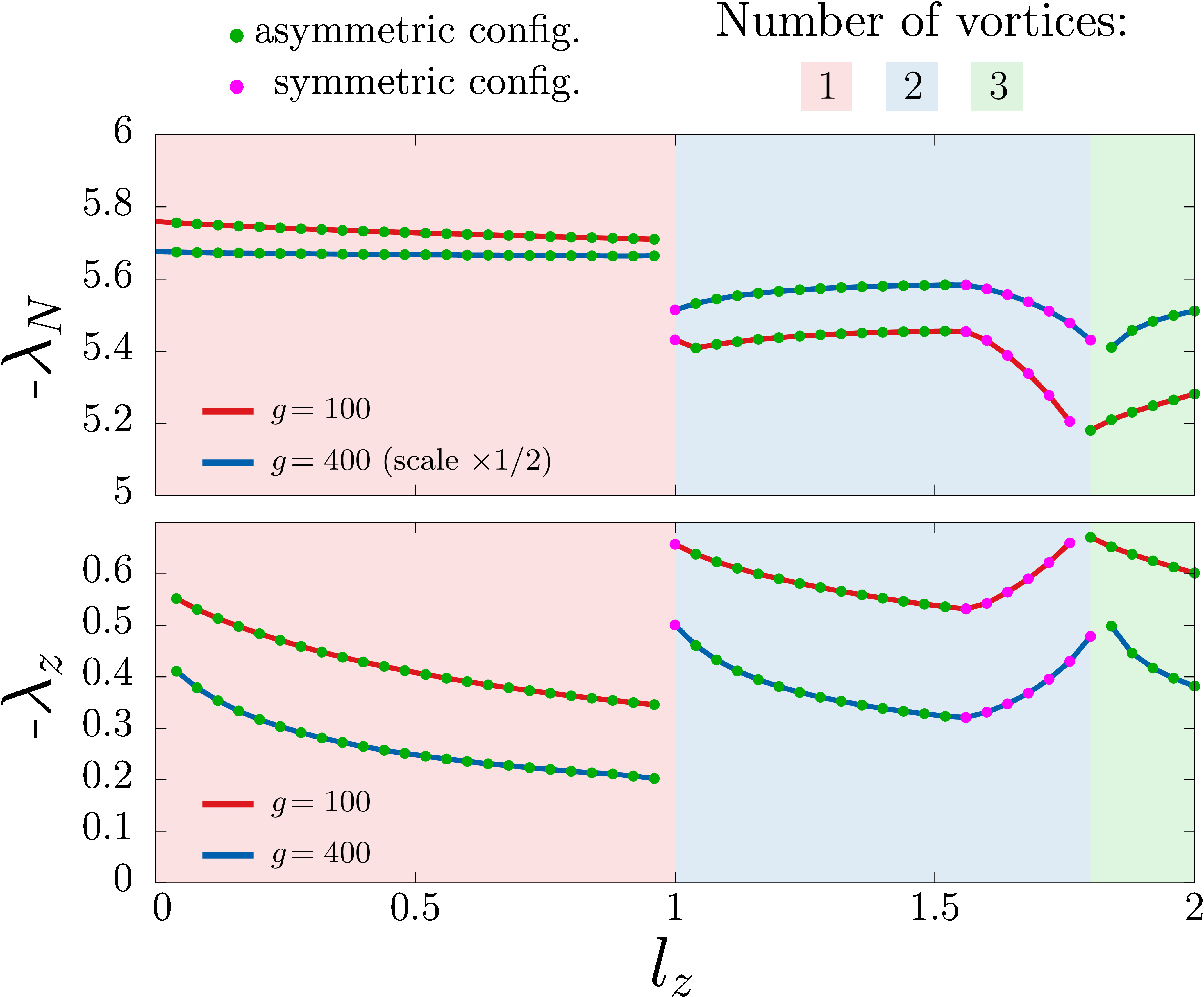
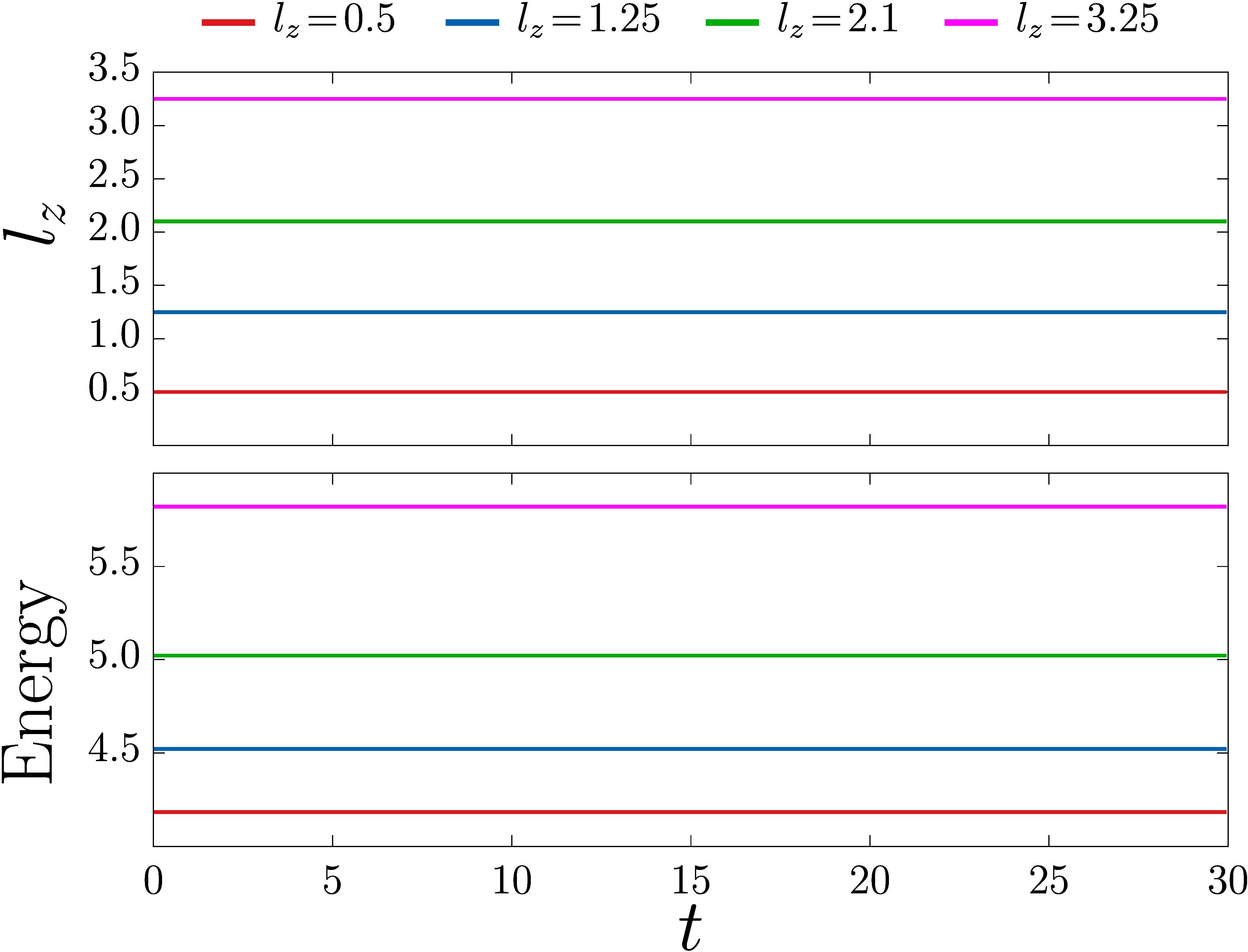
Figure 5: Details of the results of simulations where the particle number is $N=1$. The dependence of the Lagrange multipliers on the constrained angular momentum $l_{z}$ are displayed on the leftmost panel. The right panels illustrate that the time-evolution algorithm (36) used here indeed preserves the energy (bottom), the angular momentum (top) and the particle number (not shown).

Numerical minimization of the weak formulation (28) of the augmented Lagrangian (24) gives the minimal energy states under the specified values of the constraints (26). In all generality we consider unit particle number $N=1$ for various values of the angular momentum $l_{z}$. The corresponding values of the Lagrange multipliers are displayed in figure 5.

C.3 Time evolution: forward extrapolated Crank-Nicolson algorithm

To address the question of the time-dependent Gross-Pitaevskii equation, the strategy is to use a Crank-Nicolson algorithm Crank-1996 to iterate the time series. More precisely, for efficient calculations, we write a semi-implicit scheme where the nonlinear part is linearized using a forward Richardson extrapolation. The time-dependent Gross-Pitaevskii reads as:

$$i\partial_{t}\psi=-\frac{1}{2}\nabla^{2}\psi+\left[V(\mathbf{x})+g|\psi|^{2}\right]\psi\,.$$ (30)

The weak from, obtained by multiplying by test functions $\psi_{w}\in\mathcal{H}(\Omega)$ and integrating by parts reads as, in terms of the inner products (22),

$$\left\langle\psi_{w},i\partial_{t}\psi\right\rangle=\frac{1}{2}\left\langle{\boldsymbol{\nabla}}\psi_{w},{\boldsymbol{\nabla}}\psi\right\rangle+\left\langle\psi_{w},\left[V(\mathbf{x})+g|\psi|^{2}\right]\psi\right\rangle\,.$$ (31)

The discretization of the time turns the continuous evolution into a recursive series over the uniform partition $\{t\}_{n=0}^{N}$ of the time variable. The time variable is discretized as $t=n\Delta t$ and the wave function at the step $n$ is $\psi_{n}:=\psi(n\Delta t)$. The Crank-Nicolson scheme, uses (Forward-)Euler definition of the time derivative, while the r.h.s of Eq. (31) is evaluated at the averaged times. Introducing the notations

$$\partial_{t}\psi:=\delta_{t}\psi_{n}=\frac{\psi_{n+1}-\psi_{n}}{\Delta t}\,,~{}~{}\text{and}~{}~{}\bar{\psi}_{n}=\frac{\psi_{n+1}+\psi_{n}}{2}\,,$$ (32)

the Crank-Nicolson scheme for the time-dependent Gross-Pitaevskii equation (31) reads as:

$$\left\langle\psi_{w},i\delta_{t}\psi_{n}\right\rangle=\frac{1}{2}\left\langle{\boldsymbol{\nabla}}\psi_{w},{\boldsymbol{\nabla}}\bar{\psi}_{n}\right\rangle+\left\langle\psi_{w},V(\mathbf{x})\bar{\psi}_{n}\right\rangle+\left\langle\psi_{w},g|\bar{\psi}_{n}|^{2}\bar{\psi}_{n}\right\rangle\,.$$ (33)

This fully implicit scheme results in a nonlinear algebraic system which is very demanding to solve. The alternative to solving the nonlinear algebraic problem is to approximate the nonlinear part in terms of values at previous time steps. Very schematically, the idea of the modified algorithm is to approximate the fields in the nonlinear term by using an extrapolation of the previous time steps, that retains the same order of truncation error as the rest of time series. Thus, using the forward extrapolation the averaged wave function in the non-linear term becomes $\bar{\psi}_{n}\approx(3\psi_{n}-\psi_{n-1})/2$. Next, defining the time-discretized operators:

$$\mathcal{O}_{1}\psi =\left\langle\psi_{w},\frac{i\psi}{\Delta t}\right\rangle-\left\langle{\boldsymbol{\nabla}}\psi_{w},\frac{1}{4}{\boldsymbol{\nabla}}\psi\right\rangle-\left\langle\psi_{w},\frac{1}{2}V(\mathbf{x})\psi\right\rangle\,,$$ (34a)

$$\mathcal{O}_{2}\psi =\left\langle\psi_{w},\frac{i\psi}{\Delta t}\right\rangle+\left\langle{\boldsymbol{\nabla}}\psi_{w},\frac{1}{4}{\boldsymbol{\nabla}}\psi\right\rangle+\left\langle\psi_{w},\frac{1}{2}V(\mathbf{x})\psi\right\rangle\,,$$ (34b)

$$\mathcal{U}_{n}\psi =\left\langle\psi_{w},\frac{g}{8}|3\psi_{n}-\psi_{n-1}|^{2}\psi\right\rangle\,,$$ (34c)

allows to rewrite Eq. (33) in the compact form

$$\mathcal{O}_{1}\psi_{n+1}=\mathcal{O}_{2}\psi_{n}+\mathcal{U}_{n}(3\psi_{n}-\psi_{n-1})\,.$$ (35)

Hence the time-evolution is formally given by the recursion

$$\psi_{n+1}=\mathcal{O}_{1}^{-1}\big{[}\mathcal{O}_{2}\psi_{n}+\mathcal{U}_{n}(3\psi_{n}-\psi_{n-1})\big{]}\,.$$ (36)

The spatial discretization is achieved by replacing the wave function $\psi$ by its finite-element space representation $\psi^{(h)}\in V_{h}(\mathcal{T}_{h},\mathcal{P}^{(2)})$ in the time-dependent Gross-Pitaevskii equation (36). The test functions $\psi_{w}$ now take values in the same discrete space as $\psi^{(h)}$. Denoting the matrix representation of the time-discretized evolution operators (34), as:

$$\mathcal{O}_{1}\mapsto{\boldsymbol{M}}_{\psi}\,,~{}~{}~{}\mathcal{O}_{2}\mapsto{\boldsymbol{N}}_{\psi}\,,~{}~{}~{}\text{and}~{}~{}~{}~{}\mathcal{U}_{n}(3\psi_{n}-\psi_{n-1})\mapsto{\boldsymbol{R}}_{\psi}\,,$$ (37)

the recursion Eq. (36) reduce to a linear system that read as:

$$\left[{\boldsymbol{M}}_{\psi}\right]\left[\psi_{n+1}^{(h)}\right]-\left[{\boldsymbol{N}}_{\psi}\right]\left[\psi_{n}^{(h)}\right]=\left[{\boldsymbol{R}}_{\psi}\right]\,.$$ (38)

The vector ${\boldsymbol{R}}_{\psi}$ which is a function of $\psi_{n}^{(h)}$ and $\psi_{n-1}^{(h)}$, has to be recalculated at each step. The matrices ${\boldsymbol{M}}_{\psi}$ and ${\boldsymbol{N}}_{\psi}$, on the other hand, are constant matrices to be allocated just once and are in principle easily preconditioned. Finally the recursion is thus given by

$$\left[\psi_{n+1}^{(h)}\right]=\left[{\boldsymbol{M}}_{\psi}\right]^{-1}\left(\left[{\boldsymbol{N}}_{\psi}\right]\left[\psi_{n}^{(h)}\right]+\left[{\boldsymbol{R}}_{\psi}\right]\right)\,,$$ (39)

which requires recalculating the vectors ${\boldsymbol{R}}_{\psi}$ at each step and then multiplying by the inverse matrices.

The numerical simulations of the time-evolution algorithm (39) representing the discretized evolution scheme (36) accurately reproduces the intrinsic physical properties of the time-dependent Gross-Pitaevskii equation. Namely it preserves the conserved quantities like the energy, the angular momentum, and the particle number. A consistency check, as displayed on figure 5, shows that these are indeed (exactly) conserved during the time-evolution.

References

- (1) M. H. Anderson, J. R. Ensher, M. R. Matthews, C. E. Wieman and E. A. Cornell, Observation of Bose-Einstein Condensation in a Dilute Atomic Vapor, Science 269 (1995) 198.
- (2) K. B. Davis, M.-O. Mewes, M. R. Andrews, N. J. van Druten, D. S. Durfee, D. M. Kurn et al., Bose-Einstein Condensation in a Gas of Sodium Atoms, Physical Review Letters 75 (1995) 3969.
- (3) C. C. Bradley, C. A. Sackett and R. G. Hulet, Bose-Einstein Condensation of Lithium: Observation of Limited Condensate Number, Physical Review Letters 78 (1997) 985.
- (4) D. C. Aveline, J. R. Williams, E. R. Elliott, C. Dutenhoffer, J. R. Kellogg, J. M. Kohel et al., Observation of Bose–Einstein condensates in an Earth-orbiting research lab, Nature 582 (2020) 193.
- (5) E. R. Elliott, M. C. Krutzik, J. R. Williams, R. J. Thompson and D. C. Aveline, NASA’s Cold Atom Lab (CAL): system development and ground test status, npj Microgravity 4 (2018) 16.
- (6) I. Bloch, J. Dalibard and S. Nascimbène, Quantum simulations with ultracold quantum gases, Nature Physics 8 (2012) 267.
- (7) M. R. Matthews, B. P. Anderson, P. C. Haljan, D. S. Hall, C. E. Wieman and E. A. Cornell, Vortices in a Bose-Einstein Condensate, Physical Review Letters 83 (1999) 2498.
- (8) F. Chevy, K. W. Madison and J. Dalibard, Measurement of the Angular Momentum of a Rotating Bose-Einstein Condensate, Physical Review Letters 85 (2000) 2223.
- (9) C. Raman, J. R. Abo-Shaeer, J. M. Vogels, K. Xu and W. Ketterle, Vortex Nucleation in a Stirred Bose-Einstein Condensate, Physical Review Letters 87 (2001) 210402.
- (10) J. R. Abo-Shaeer, C. Raman, J. M. Vogels and W. Ketterle, Observation of Vortex Lattices in Bose-Einstein Condensates, Science 292 (2001) 476.
- (11) E. P. Gross, Structure of a quantized vortex in boson systems, Il Nuovo Cimento 20 (1961) 454.
- (12) L. P. Pitaevskii, Vortex Lines in an Imperfect Bose Gas , Soviet Journal of Experimental and Theoretical Physics 13 (1961) 451.
- (13) L. P. Pitaevskii and S. Stringari, Bose-Einstein condensation, no. 116 in International series of monographs on physics. Clarendon Press, Oxford New York, 2003.
- (14) E. H. Lieb and R. Seiringer, Derivation of the Gross-Pitaevskii Equation for Rotating Bose Gases, Communications in Mathematical Physics 264 (2006) 505.
- (15) C. J. Pethick and H. Smith, Bose–Einstein Condensation in Dilute Gases. Cambridge University Press, ii ed., 2008, 10.1017/CBO9780511802850.
- (16) A. L. Fetter, Rotating trapped Bose-Einstein condensates, Reviews of Modern Physics 81 (2009) 647.
- (17) W. Bao and Y. Cai, Mathematical theory and numerical methods for Bose-Einstein condensation, Kinetic & Related Models 6 (2013) 1.
- (18) P. C. Haljan, I. Coddington, P. Engels and E. A. Cornell, Driving Bose-Einstein-Condensate Vorticity with a Rotating Normal Cloud, Physical Review Letters 87 (2001) 210403.
- (19) A. L. Fetter and A. A. Svidzinsky, Vortices in a trapped dilute Bose-Einstein condensate, Journal of Physics: Condensed Matter 13 (2001) R135.
- (20) D. A. Butts and D. S. Rokhsar, Predicted signatures of rotating Bose–Einstein condensates, Nature 397 (1999) 327.
- (21) A. Aftalion and Q. Du, Vortices in a rotating Bose-Einstein condensate: Critical angular velocities and energy diagrams in the Thomas-Fermi regime, Physical Review A 64 (2001) 063603.
- (22) R. Seiringer, Gross-Pitaevskii Theory of the Rotating Bose Gas, Communications in Mathematical Physics 229 (2002) 491.
- (23) B. P. Anderson, P. C. Haljan, C. E. Wieman and E. A. Cornell, Vortex Precession in Bose-Einstein Condensates: Observations with Filled and Empty Cores, Physical Review Letters 85 (2000) 2857.
- (24) R. Fletcher, Practical Methods of Optimization. Wiley, Chichester New York, 1987, 10.1002/9781118723203.
- (25) J. Nocedal and S. J. Wright, Numerical Optimization, Springer Series in Operations Research. Springer, 1999, 10.1007/978-0-387-40065-5.
- (26) B. Mottelson, Yrast Spectra of Weakly Interacting Bose-Einstein Condensates, Physical Review Letters 83 (1999) 2695.
- (27) G. M. Kavoulakis, B. Mottelson and C. J. Pethick, Weakly interacting Bose-Einstein condensates under rotation, Physical Review A 62 (2000) 063605.
- (28) A. Shapere and F. Wilczek, Classical Time Crystals, Physical Review Letters 109 (2012) 160402.
- (29) F. Wilczek, Quantum Time Crystals, Physical Review Letters 109 (2012) 160401.
- (30) A. Alekseev, J. Dai and A. J. Niemi, Provenance of classical Hamiltonian time crystals, Journal of High Energy Physics 2020 (2020) 35.
- (31) J. Dai, A. J. Niemi and X. Peng, Classical Hamiltonian time crystals – general theory and simple examples, New Journal of Physics 22 (2020) 085006.
- (32) J. M. Leinaas and J. Myrheim, On the Theory of Identical Particles, Il Nuovo Cimento B 37 (1977) 1.
- (33) F. Wilczek, Quantum Mechanics of Fractional-Spin Particles, Physical Review Letters 49 (1982) 957.
- (34) R. Iengo and K. Lechne, Anyon quantum mechanics and Chern-Simons theory, Physics Reports 213 (1992) 179.
- (35) A. Lerda, Anyons : quantum mechanics of particles with fractional statistics, vol. 14 of Lecture Notes in Physics. Lecture Notes in Physics, Berlin New York, 1992, 10.1007/978-3-540-47466-1.
- (36) A. Y. Kitaev, Fault-tolerant quantum computation by anyons , Annals of Physics 303 (2003) 2.
- (37) J. Nakamura, S. Liang, G. C. Gardner and M. J. Manfra, Direct observation of anyonic braiding statistics, Nature Physics 16 (2020) 931.
- (38) E. H. Lieb and R. Seiringer, Proof of Bose-Einstein Condensation for Dilute Trapped Gases, Physical Review Letters 88 (2002) 170409.
- (39) J. E. Marsden and T. S. Ratiu, Introduction to Mechanics and Symmetry. Springer New York, New York, 1999, 10.1007/978-0-387-21792-5.
- (40) F. Hecht, New development in freefem++, Journal of Numerical Mathematics 20 (2012) 251.
- (41) see Supplementary Materials for animations.
- (42) F. Wilczek, Magnetic Flux, Angular Momentum, and Statistics, Physical Review Letters 48 (1982) 1144.
- (43) K.-P. Marzlin, W. Zhang and E. M. Wright, Vortex Coupler for Atomic Bose-Einstein Condensates, Physical Review Letters 79 (1997) 4728.
- (44) E. L. Bolda and D. F. Walls, Creation of vortices in a Bose-Einstein condensate by a Raman technique, Physics Letters A 246 (1998) 32.
- (45) R. Dum, J. I. Cirac, M. Lewenstein and P. Zoller, Creation of Dark Solitons and Vortices in Bose-Einstein Condensates, Physical Review Letters 80 (1998) 2972.
- (46) A. E. Leanhardt, A. Görlitz, A. P. Chikkatur, D. Kielpinski, Y. Shin, D. E. Pritchard et al., Imprinting Vortices in a Bose-Einstein Condensate using Topological Phases, Physical Review Letters 89 (2002) .
- (47) T. W. B. Kibble, Topology of Cosmic Domains and Strings, Journal of Physics A: Mathematical and General 9 (1976) 1387.
- (48) W. H. Zurek, Cosmological experiments in superfluid helium?, Nature 317 (1985) 505.
- (49) W. H. Zurek, Cosmological experiments in condensed matter systems, Physics Reports 276 (1996) 177.
- (50) J. R. Anglin and W. H. Zurek, Vortices in the Wake of Rapid Bose-Einstein Condensation, Physical Review Letters 83 (1999) 1707.
- (51) V. M. H. Ruutu, V. B. Eltsov, A. J. Gill, T. W. B. Kibble, M. Krusius, Y. G. Makhlin et al., Vortex formation in neutron-irradiated superfluid 3He as an analogue of cosmological defect formation, Nature 382 (1996) 334.
- (52) V. B. Eltsov, T. W. B. Kibble, M. Krusius, V. M. H. Ruutu and G. E. Volovik, Composite Defect Extends Analogy between Cosmology and 3He, Physical Review Letters 85 (2000) 4739.
- (53) C. N. Weiler, T. W. Neely, D. R. Scherer, A. S. Bradley, M. J. Davis and B. P. Anderson, Spontaneous vortices in the formation of Bose-Einstein condensates, Nature 455 (2008) 948.
- (54) D. V. Freilich, D. M. Bianchi, A. M. Kaufman, T. K. Langin and D. S. Hall, Real-Time Dynamics of Single Vortex Lines and Vortex Dipoles in a Bose-Einstein Condensate, Science 329 (2010) 1182.
- (55) D. V. Hutton, Fundamentals of Finite Element Analysis, Engineering Series. McGraw-Hill, 2003, 10.1036/0072922362.
- (56) J. Reddy, An Introduction to the Finite Element Method. McGraw-Hill Education, 2005.
- (57) P. E. Gill, W. Murray and M. H. Wright, Practical optimization. Academic Press, 1981.
- (58) E. G. Birgin and J. M. Martínez, Improving ultimate convergence of an augmented Lagrangian method, Optimization Methods and Software 23 (2008) 177.
- (59) M. R. Hestenes and E. Stiefel, Methods of conjugate gradients for solving linear systems, Journal of Research of the National Bureau of Standards 49 (1952) 409.
- (60) R. Fletcher and C. M. Reeves, Function minimization by conjugate gradients, The Computer Journal 7 (1964) 149.
- (61) E. Polak and G. Ribière, Note sur la convergence de directions conjuguées, Revue française d’informatique et de recherche opérationnelle. Série rouge 3 (1969) 35.
- (62) J. Crank and P. Nicolson, A practical method for numerical evaluation of solutions of partial differential equations of the heat-conduction type, Advances in Computational Mathematics 6 (1996) 207.