Online Back-Parsing for AMR-to-Text Generation

Abstract

AMR-to-text generation aims to recover a text containing the same meaning as an input AMR graph. Current research develops increasingly powerful graph encoders to better represent AMR graphs, with decoders based on standard language modeling being used to generate outputs. We propose a decoder that back predicts projected AMR graphs on the target sentence during text generation. As the result, our outputs can better preserve the input meaning than standard decoders. Experiments on two AMR benchmarks show the superiority of our model over the previous state-of-the-art system based on graph Transformer.

1 Introduction

Abstract meaning representation (AMR) Banarescu et al. (2013) is a semantic graph representation that abstracts meaning away from a sentence. Figure 1 shows an AMR graph, where the nodes, such as “possible-01” and “police”, represent concepts, and the edges, such as “ARG0” and “ARG1”, indicate relations between the concepts they connect. The task of AMR-to-text generation Konstas et al. (2017) aims to produce fluent sentences that convey consistent meaning with input AMR graphs. For example, taking the AMR in Figure 1 as input, a model can produce the sentence “The police could help the victim”. AMR-to-text generation has been shown useful for many applications such as machine translation Song et al. (2019) and summarization Liu et al. (2015); Yasunaga et al. (2017); Liao et al. (2018); Hardy and Vlachos (2018). In addition, AMR-to-text generation can be a good test bed for general graph-to-sequence problems Belz et al. (2011); Gardent et al. (2017).

AMR-to-text generation has attracted increasing research attention recently. Previous work has focused on developing effective encoders for representing graphs. In particular, graph neural networks Beck et al. (2018); Song et al. (2018); Guo et al. (2019) and richer graph representations Damonte and Cohen (2019); Hajdik et al. (2019); Ribeiro et al. (2019) have been shown to give better performances than RNN-based models Konstas et al. (2017) on linearized graphs. Subsequent work exploited graph Transformer Zhu et al. (2019); Cai and Lam (2020); Wang et al. (2020), achieving better performances by directly modeling the intercorrelations between distant node pairs with relation-aware global communication. Despite the progress on the encoder side, the current state-of-the-art models use a rather standard decoder: it functions as a language model, where each word is generated given only the previous words. As a result, one limitation of such decoders is that they tend to produce fluent sentences that may not retain the meaning of input AMRs.

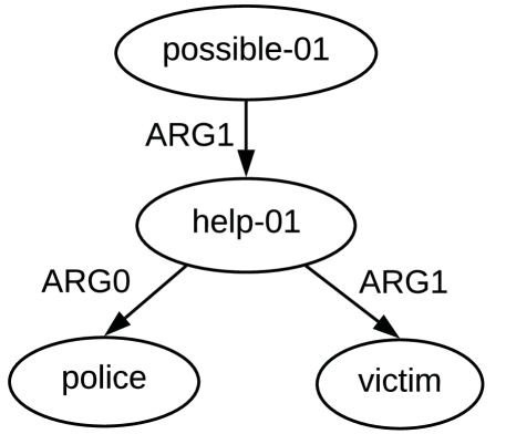
Figure 1: An example AMR graph meaning “The police could help the victim.”

We investigate enhancing AMR-to-text decoding by integrating online back-parsing, simultaneously predicting a projected AMR graph on the target sentence while it is being constructed. This is largely inspired by work on back-translation Sennrich et al. (2016); Tu et al. (2017), which shows that back predicting the source sentence given a target translation output can be useful for strengthening neural machine translation. We perform online back parsing, where the AMR graph structure is constructed through the autoregressive sentence construction process, thereby saving the need for training a separate AMR parser. By adding online back parsing to the decoder, structural information of the source graph can intuitively be better preserved in the decoder network.

Figure 2 visualizes our structure-integrated decoding model when taking the AMR in Figure 1 as input. In particular, at each decoding step, the model predicts the current word together with its corresponding AMR node and outgoing edges to the previously generated words. The predicted word, AMR node and edges are then integrated as the input for the next decoding step. In this way, the decoder can benefit from both more informative loss via multi-task training and richer features taken as decoding inputs.

Experiments on two AMR benchmark datasets (LDC2015E86 and LDC2017T10) show that our model significantly outperforms a state-of-the-art graph Transformer baseline by 1.8 and 2.5 BLEU points, respectively, demonstrating the advantage of structure-integrated decoding for AMR-to-text generation. Deep analysis and human evaluation also confirms the superiority of our model. Our code is available at https://github.com/muyeby/AMR-Backparsing.

2 Baseline: Graph Transformer

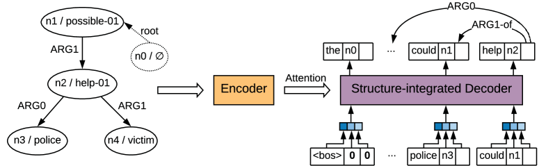
Figure 2: Overview of the proposed model.

Formally, the AMR-to-text generation task takes an AMR graph as input, which can be denoted as a directed acyclic graph $G=(V,E)$, where $V$ denotes the set of nodes and $E$ refers to the set of labeled edges. An edge can further be represented by a triple $\left\langle v_{i},{r_{k}},v_{j}\right\rangle$, showing that node $v_{i}$ and $v_{j}$ are connected by relation type $r_{k}$. Here $k\in[1,...,R]$, and $R$ is the total number of relation types. The goal of AMR-to-text generation is to generate a word sequence $\textbf{y}=[y_{1},y_{2},\dots,y_{M}]$, which conveys the same meaning as $G$.

We take a graph Transformer model Koncel-Kedziorski et al. (2019); Zhu et al. (2019); Cai and Lam (2020); Wang et al. (2020) as our baseline. Previous work has proposed several variations of graph-Transformer. We take the model of Zhu et al. (2019), which gives the state-of-the-art performance. This approach exploits a graph Transformer encoder for AMR encoding and a standard Transformer decoder for text generation.

2.1 Graph Transformer Encoder

The Graph Transformer Encoder is an extension of the standard Transformer encoder Vaswani et al. (2017), which stacks $L$ encoder layers, each having two sublayers: a self-attention layer and a position-wise feed forward layer. Given a set of AMR nodes $[v_{1},v_{2},\dots,v_{N}]$, the $l$-th encoder layer takes the node features $[h_{1}^{l-1},h_{2}^{l-1},\dots,h_{N}^{l-1}]$ from its preceding layer as input and produces a new set of features $[h_{1}^{l},h_{2}^{l},\dots,h_{N}^{l}]$ as its output. Here $h_{i}^{l-1},h_{i}^{l}\in\mathcal{R}^{d}$, $d$ is the feature dimension, $l\in[1,\dots,L]$, and $h_{i}^{0}$ represents the embedding of AMR node $v_{i}$, which is randomly initialized.

The graph Transformer encoder extends the vanilla self-attention (SAN) mechanism by explicitly encoding the relation $r_{k}$ between each AMR node pair $(v_{i},v_{j})$ in the graph. In particular, the relation-aware self-attention weights are obtained by:

$$\begin{split}\alpha_{ij}&=\frac{\exp(e_{ij})}{\sum\nolimits_{n\in[1,\dots,N]}\exp{(e_{in})}},\\ e_{ij}&=\frac{(W^{Q}h_{i}^{l-1})^{T}(W^{K}h_{j}^{l-1}+W^{R}\gamma_{k})}{\sqrt{d}},\\ \end{split}$$ (1)

where $W^{Q},W^{K},W^{R}$ are model parameters, and $\gamma_{k}\in\mathcal{R}^{d_{r}}$ is the embedding of relation $r_{k}$, which is randomly initialized and optimized during training, $d_{r}$ is the dimension of relation embeddings.

With $\alpha_{ij}$, the output features are:

$$h^{l}_{i}=\sum\nolimits_{j\in[1,\dots,N]}\alpha_{ij}(W^{V}{h}^{l-1}_{j}+W^{R}\gamma_{k}),$$ (2)

where $W^{V}$ is a parameter matrix.

Similar to the vanilla Transformer, a graph Transformer also uses multi-head self-attention, residual connection and layer normalization.

2.2 Standard Transformer Decoder

The graph Transformer decoder is identical to the vanilla Transformer Vaswani et al. (2017). It consists of an embedding layer, multiple Transformer decoder layers and a generator layer (parameterized with a linear layer followed by softmax activation). Supposing that the number of decoder layers is the same as the encoder layers, denoted as $L$. The decoder consumes the hidden states of the top-layer encoder $H^{L}=[h_{1}^{L},h_{2}^{L},\dots,h_{N}^{L}]$ as input and generates a sentence $\textbf{y}=[y_{1},y_{2},\dots,y_{M}]$ word-by-word, according to the hidden states of the topmost decoder layer $S^{L}=[s^{L}_{1},s^{L}_{2},\dots,s^{L}_{M}]$.

Formally, at time $t$, the $l$-th decoder layer ($l\in[1,\dots,L]$) updates the hidden state as:

$$\begin{split}\hat{s}_{t}^{l}&=\text{SAN}(s_{1}^{l-1},s_{2}^{l-1},\dots,s_{t}^{l-1}),\\ c_{t}^{l}&=\text{AN}(\hat{s}_{t}^{l},H^{L}),\\ s^{l}_{t}&=\text{FF}(c_{t},\hat{s}_{t}^{l}),\\ \end{split}$$ (3)

where FF denotes a position-wise feed-forward layer, $[s_{1}^{l-1},s_{2}^{l-1},\dots,s_{t}^{l-1}]$ represent the hidden states of the $l-1$th decoder layer, $[s^{0}_{1},s^{0}_{2},\dots,s^{0}_{t}]$ are embeddings of $[y_{s},y_{1},\dots,y_{t-2},y_{t-1}]$, and $y_{s}$ denotes the start symbol of a sentence.

In Eq 3, AN is a standard attention layer, which computes a set of attention scores $\beta_{ti}(i\in{[1,\dots,N]})$ and a context vector $c_{t}$:

$$\begin{split}\beta_{ti}&=\frac{\exp(f({\hat{s}_{t}^{l},h_{i}^{L}}))}{\sum\nolimits_{j\in[1,\dots,N]}\exp{(f({\hat{s}_{t}^{l},h_{j}^{L}}))}},\\ c^{l}_{t}&=\sum\nolimits_{i\in[1,\dots,N]}\beta_{ti}h_{i}^{L},\end{split}$$ (4)

where $f$ is a scaled dot-product attention function.

Denoting the output hidden state of the $L$-th decoder layer at time $t$ as $s_{t}^{L}$, the generator layer predicted the probability of a target word $y_{t}$ as:

$$p(y_{t}|\textbf{y}_{<t},G)=\text{softmax}(W_{g}s_{t}^{L}),$$ (5)

where $\textbf{y}_{<t}=[y_{1},y_{2},\dots,y_{t-1}]$, and $W_{g}$ is a model parameter.

2.3 Training Objective

The training objective of the baseline model is to minimize the negative log-likelihood of conditional word probabilities:

$$\begin{split}\ell_{std}&=-\sum\nolimits_{t\in[1,\dots,M]}log~{}p(y_{t}|\textbf{y}_{<t},G)\\ &=-\sum\nolimits_{t\in[1,\dots,M]}log~{}p({y_{t}|s_{t}^{L};\Theta}),\\ \end{split}$$ (6)

where $\Theta$ denotes the full set of parameters.

3 Model with Back-Parsing

Figure 2 illustrates the proposed model. We adopt the baseline graph encoder described in Section 2.1 for AMR encoding, while enhancing the baseline decoder (Section 2.2) with AMR graph prediction for better structure preservation. In particular, we train the decoder to reconstruct the AMR graph (so called “back-parsing”) by jointly predicting the corresponding AMR nodes and projected relations when generating a new word. In this way, we expect that the model can better memorize the AMR graph and generate more faithful outputs. In addition, our decoder is trained in an online manner, which uses the last node and edge predictions to better inform the generation of the next word.

Specifically, the encoder hidden states are first calculated given an AMR graph. At each decoding time step, the proposed decoder takes the encoder states as inputs and generates a new word (as in Section 2.2), together with its corresponding AMR node (Section 3.1) and its outgoing edges (Section 3.2), These predictions are then used inputs to calculate the next state (Section 3.3).

3.1 Node Prediction

We first equip a standard decoder with the ability to make word-to-node alignments while generating target words. Making alignments can be formalized as a matching problem, which aims to find the most relevant AMR graph node for each target word. Inspired by previous work Liu et al. (2016); Mi et al. (2016), we solve the matching problem by supervising the word-to-node attention scores given by the Transformer decoder. In order to deal with words without alignments, we introduce a NULL node $v_{\emptyset}$ into the input AMR graph (as shown in Figure 2) and align such words to it.

More specifically, at each decoding step $t$, our Transformer decoder first calculates the top decoder layer word-to-node attention distribution $\beta_{t}^{\prime}=[\beta_{t0}^{\prime},\beta_{t1}^{\prime},...,\beta_{tN}^{\prime}]$ (Eq 3 and Eq 4) after taking the encoder states $H^{L}=[h_{0}^{L},h_{1}^{L},h_{2}^{L},\dots,h_{N}^{L}]$ together with the previously generated sequence $\textbf{y}_{<t}=[y_{1},y_{2},\dots,y_{t-1}]$ ($\beta_{t0}^{\prime}$ and $h_{0}^{L}$ are the probability and encoder state for the NULL node $v_{\emptyset}$). Then the probability of aligning the current decoder state to node $v_{i}$ is defined as:

$$\begin{split}p(\texttt{ALI}(s_{t})=v_{i}|H^{L},\textbf{y}_{<t})=\beta_{ti}^{\prime},\\ \end{split}$$ (7)

where ALI is the sub-network for finding the best aligned AMR node for a given decoder state.

Training. Supposing that the gold alignment (refer to Section 4.1) at time $t$ is $\hat{\beta}_{t}$, the training objective for node prediction is to minimize the loss defined as the distance between $\beta_{t}^{\prime}$ and $\hat{\beta}_{t}$:

$$\begin{split}\ell_{node}=\sum\nolimits_{t\in[1,\dots,M]}\Delta(\beta_{t}^{\prime},\hat{\beta_{t}}),\\ \end{split}$$ (8)

where $\Delta$ denotes a discrepancy criterion that can quantify the distance between $\beta_{t}^{\prime}$ and $\hat{\beta_{t}}$. We take two common alternatives: (1) Mean Squared Error (MSE), and (2) Cross Entropy Loss (CE).

3.2 Edge Prediction

The edge prediction sub-task aims to preserve the node-to-node relations in an AMR graph during text generation. To this end, we project the edges of each input AMR graph onto the corresponding sentence according to their node-to-word alignments, before training the decoder to generate the projected edges along with target words. For words without outgoing edges, we add a “self-loop” edge for consistency.

Formally, at decoding step $t$, each relevant directed edge (or arc) with relation label $r_{k}$ starting from $y_{t}$ can be represented as $\left\langle y_{j},r_{k},y_{t}\right\rangle$, where $j\leq t$, $y_{j}$, $y_{t}$ and $r_{k}$ are called “arc_to”, “arc_from”, and “label” respectively. We modify the deep biaffine attention classifier Dozat and Manning (2016) to model these edges. In particular, we factorize the probability for each labeled edge into the “arc” and “label” parts, computing both based on the current decoder hidden state and the states of all previous words. The “arc” score $\psi^{\text{arc}}_{tj}\in\mathcal{R}^{1}$, which measures whether or not a directed edge from $y_{t}$ to $y_{j}$ exists, is calculated as:

$$\begin{split}&b_{j}^{\text{arc\_to}},b_{t}^{\text{arc\_from}}=\text{FF}^{\text{arc\_to}}(s_{j}^{L}),\text{FF}^{\text{arc\_from}}(s_{t}^{L}),\\ &\hat{\psi}^{\text{arc}}_{tj}=\text{Biaff}^{\text{arc}}(b_{j}^{\text{arc\_to}},b_{t}^{\text{arc\_from}}),\\ &\psi^{\text{arc}}_{t1},\psi^{\text{arc}}_{t2},...,\psi^{\text{arc}}_{tj},...,\psi^{\text{arc}}_{tt}\\ &\quad~{}~{}=\text{softmax}(\hat{\psi}^{\text{arc}}_{t1},\hat{\psi}^{\text{arc}}_{t2},...,\hat{\psi}^{\text{arc}}_{tj},...,\hat{\psi}^{\text{arc}}_{tt}).\\ \end{split}$$ (9)

Similarly, the “label” score $\psi^{\text{label}}_{tj}\in\mathcal{R}^{R}$, which is used to predict a label for potential word pair ($y_{j}$, $y_{t}$), is given by:

$$\begin{split}b_{j}^{\text{label\_to}},&b_{t}^{\text{label\_from}}=\text{FF}^{\text{label\_to}}(s_{j}^{L}),\text{FF}^{\text{label\_from}}(s_{t}^{L}),\\ \psi^{\text{label}}_{tj}&=\text{softmax}\big{(}\text{Biaff}^{\text{label}}(b_{j}^{\text{label\_to}},b_{t}^{\text{label\_from}})\big{)}.\\ \end{split}$$ (10)

In Eq 9 and Eq 10, $\text{FF}^{\text{arc\_to}}$, $\text{FF}^{\text{arc\_from}}$, $\text{FF}^{\text{label\_to}}$ and $\text{FF}^{\text{label\_from}}$ are linear transformations. $\text{Biaff}^{\text{arc}}$ and $\text{Biaff}^{\text{label}}$ are biaffine transformations:

$$\begin{split}\text{Biaff}(x_{1},x_{2})=x_{1}^{T}Ux_{2}+W(x_{1}\oplus x_{2})+b,\end{split}$$ (11)

where $\oplus$ denotes vector concatenation, $U,W$ and $b$ are model parameters. $U$ is a $(d\times 1\times d)$ tensor for unlabeled classification (Eq 9) and a $(d\times R\times d)$ tensor for labeled classification (Eq 10), where $d$ is the hidden size.

Defining $p(y_{j}|y_{t})$ as $\psi^{\text{arc}}_{tj}$ and $p(r_{k}|y_{j},y_{t})$ as $\psi^{\text{label}}_{tj}[k]$, the probability of a labeled edge $\left\langle y_{j},r_{k},y_{t}\right\rangle$ is calculated by the chain rule:

$$\begin{split}p(r_{k},y_{j}|y_{t})&=p(r_{k}|y_{j},y_{t})p(y_{j}|y_{t})\\ &=\psi^{\text{label}}_{tj}[k]\cdot\psi^{\text{arc}}_{tj}.\\ \end{split}$$ (12)

Training. The training objective for the edge prediction task is the negative log-likelihood over all projected edges ${E^{\prime}}$:

$$\begin{split}\ell_{label}&=-\sum\nolimits_{\left\langle y_{j},r_{k},y_{i}\right\rangle\in E^{\prime}}log~{}p(r_{k},y_{j}|y_{i})\\ \end{split}$$ (13)

3.3 Next State Calculation

In addition to simple “one-way” AMR back-parsing (as shown in Section 3.1 and 3.2), we also study integrating the previously predicted AMR nodes and outgoing edges as additional decoder inputs to help generate the next word. In particular, for calculating the decoder hidden states $[s^{1}_{t+1},s^{2}_{t+1},...,s^{L}_{t+1}]$ at step $t+1$, the input feature to our decoder is a triple $\left\langle\vec{y}_{t},\vec{v}_{t},\vec{e}_{t}\right\rangle$ instead of a single value $\vec{y}_{t}$, which the baseline has. Here $\vec{y}_{t},\vec{v}_{t}$ and $\vec{e}_{t}$ are vector representations of the predicted word, AMR node and edges at step $t$, respectively. More specifically, $\vec{v}_{t}$ is a weighted sum of the top-layer encoder hidden states $[h_{0}^{L},h_{1}^{L},...,h_{N}^{L}]$, and coefficients are from the distribution of $\beta^{\prime}_{t}$ in Eq 7:

$$\begin{split}\vec{v}_{t}&=\sum\nolimits_{i\in[0,\dots,N]}\beta^{\prime}_{ti}\odot h_{i}^{L},\\ \end{split}$$ (14)

where $\odot$ is the operation for scalar-tensor product.

Similarly, $\vec{e}_{t}$ is calculated as:

$$\begin{split}\vec{e}_{t}&=\vec{r}_{t}\oplus\vec{s}_{t},\\ \vec{r}_{t}&=\sum\nolimits_{k=1}^{|R|}\sum\nolimits_{j=1}^{t}p(r_{k},y_{j}|y_{t})\gamma_{k},\\ \vec{s}_{t}&=\sum\nolimits_{j=1}^{t}p(y_{j}|y_{t})s^{L}_{j},\\ \end{split}$$ (15)

where $\oplus$ concatenates two tensors, $p(r_{k},y_{j}|y_{t})$ and $p(y_{j}|y_{t})$ are probabilities given in Eq 12, $\gamma_{k}$ is a relation embedding, and $s^{L}_{j}$ is the decoder hidden state at step $j$. $\vec{e}_{t-1}$ is a vector concatenation of $\vec{r}_{t}$ and $\vec{s}_{t}$, which are weighted sum of relation embeddings and weighted sum of previous decoder hidden states, respectively.

In contrast to the baseline in Eq 3, at time t+1, the hidden state of the first decoder layer is calculated as:

$$\begin{split}\hat{s}_{t+1}^{1}&=\text{SAN}(s_{1}^{0},...,s_{t}^{0},\vec{y}_{t},\vec{v}_{t},\vec{e}_{t}),\\ c_{t+1}^{1}&=\text{AN}(\hat{s}_{t+1}^{1},H^{L}),\\ s^{1}_{t+1}&=\text{FF}(c_{t+1}^{1},\hat{s}_{t+1}^{1}),\\ \end{split}$$ (16)

where the definition of $H^{L}$, SAN, AN, FF and $[s^{0}_{1},\dots,s^{0}_{t}]$ are the same as Eq 3. $\vec{v}_{0}$ and $\vec{e}_{0}$ (as shown in Figure 2) are defined as zero vectors. The hidden states of upper decoder layers ($[s^{2}_{t+1},...,s^{L}_{t+1}]$) are updated in the same way as Eq 3.

Following previous work on syntactic text generation Wu et al. (2017); Wang et al. (2018), we use gold AMR nodes and outgoing edges as inputs for training, while we take automatic predictions for decoding.

3.4 Training Objective

The overall training objective is:

$$\begin{split}\ell_{total}&=\ell_{std}+\lambda_{1}\ell_{node}+\lambda_{2}\ell_{label},\\ \end{split}$$ (17)

where $\lambda_{1}$ and $\lambda_{2}$ are weighting hyper-parameters for $\ell_{node}$ and $\ell_{label}$, respectively.

4 Experiments

We conduct experiments on two benchmark AMR-to-text generation datasets, including LDC2015E86 and LDC2017T10. These two datasets contain 16,833 and 36,521 training examples, respectively, and share a common set of 1,368 development and 1,371 test instances.

4.1 Experimental Settings

Data preprocessing. Following previous work Song et al. (2018); Zhu et al. (2019), we take a standard simplifier Konstas et al. (2017) to preprocess AMR graphs, adopting the Stanford tokenizer and Subword Tool to segment text into subword units. The node-to-word alignments are generated by ISI aligner Pourdamghani et al. (2014). We then project the source AMR graph onto the target sentence according to such alignments.

For node prediction, the attention distributions are normalized, but the alignment scores generated by the ISI aligner are unnormalized hard $0/1$ values. To enable cross entropy loss, we follow previous work Mi et al. (2016) to normalize the gold-standard alignment scores.

Hyperparameters. We choose the feature-based model of Zhu et al. (2019) as our baseline (G-Trans-F-Ours). Also following their settings, both the encoder and decoder have $6$ layers, with each layer having $8$ attention heads. The sizes of hidden layers and word embeddings are $512$, and the size of relation embedding is $64$. The hidden size of the biaffine attention module is 512. We use Adam Kingma and Ba (2015) with a learning rate of 0.5 for optimization. Our models are trained for 500K steps on a single 2080Ti GPU. We tune these hyperparameters on the LDC2015E86 development set and use the selected values for testing.

Model Evaluation. We set the decoding beam size as $5$ and take BLEU Papineni et al. (2002) and Meteor Banerjee and Lavie (2005); Denkowski and Lavie (2014) as automatic evaluation metrics. We also employ human evaluation to assess the semantic faithfulness and generation fluency of compared methods by randomly selecting 50 AMR graphs for comparison. Three people familiar with AMR are asked to score the generation quality with regard to three aspects — concept preservation rate, relation preservation rate and fluency (on a scale of [0, 5]). Details about the criteria are:

• Concept preservation rate assesses to what extent the concepts in input AMR graphs are involved in generated sentences.
• Relation preservation rate measures to what extent the relations in input AMR graphs exist in produced utterances.
• Fluency evaluates whether the generated sentence is fluent and grammatically correct.

Recently, significant progress  Ribeiro et al. (2019); Zhang et al. (2020); Çelikyilmaz et al. (2020) in developing new metrics for NLG evaluation has made. We leave evaluation on these metrics for future work.

4.2 Development Experiments

Model	BLEU	Meteor
G-Trans-F-Ours	30.20	35.23
Node Prediction MSE	30.66	35.60
Node Prediction CE	30.85	35.71
Edge Prediction share	31.19	35.75
Edge Prediction independent	31.13	35.69

Table 1: BLEU and Meteor scores on the LDC2015E86 devset under different model settings.

Table 1 shows the performances on the devset of LDC2015E86 under different model settings. For the node prediction task, it can be observed that both cross entropy loss (CE) and mean squared error loss (MSE) give significantly better results than the baseline, with 0.46 and 0.65 improvement in terms of BLEU, respectively. In addition, CE gives a better result than MSE.

Regarding edge prediction, we investigate two settings, with relation embeddings being shared by the encoder and decoder, or being separately constructed, respectively. Both settings give large improvements over the baseline. Compared with the model using independent relation embeddings, the model with shared relation embeddings gives slightly better results with less parameters, indicating that the relations in an AMR graph and the relations between words are consistent. We therefore adopt the CE loss and shared relation embeddings for the remaining experiments.

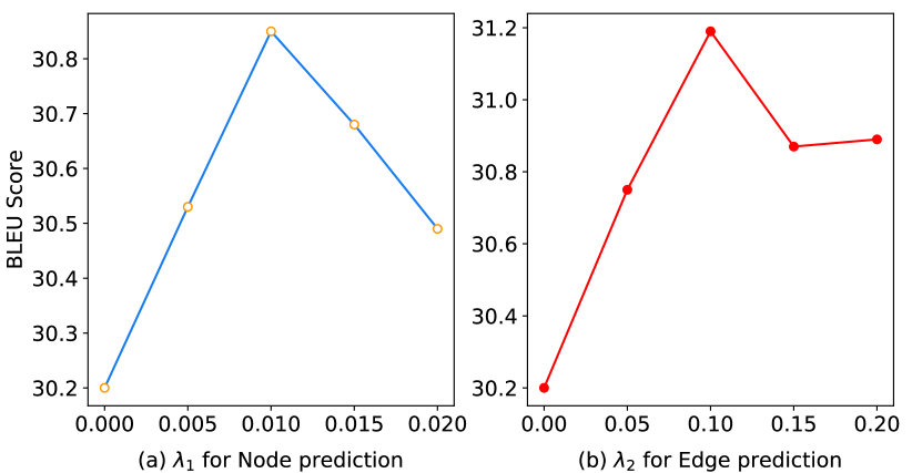
Figure 3: BLEU scores on the LDC2015E86 devset against different hyperparameter values.

Figure 3 presents the BLEU scores of integrating standard AMR-to-text generation with node prediction or edge prediction under different $\lambda_{1}$ and $\lambda_{2}$ values, respectively. There are improvements when increasing the coefficient from $0$, demonstrating that both node prediction and edge prediction have positive influence on AMR-to-text generation. The BLEU of the two models reach peaks at $\lambda_{1}=0.01$ and $\lambda_{2}=0.1$, respectively. When further increasing the coefficients, the BLEU scores start to decrease. We thus set $\lambda_{1}=0.01,\lambda_{2}=0.1$ for the rest of our experiments.

4.3 Main Results

4.3.1 Automatic Evaluation

Model	LDC15	LDC17
LSTM Konstas et al. (2017)	22.00	–
GGNN Beck et al. (2018)	–	23.30
GRN Song et al. (2018)	23.30	–
DCGCN Guo et al. (2019)	25.9	27.9
G-Trans-F Zhu et al. (2019)	27.23	30.18
G-Trans-SA Zhu et al. (2019)	29.66	31.54
G-Trans-C Cai and Lam (2020)	27.4	29.8
G-Trans-W Wang et al. (2020)	25.9	29.3
G-Trans-F-Ours	30.15	31.53
Ours Back-Parsing	31.48	34.19
with external data
LSTM (20M) Konstas et al. (2017)	33.8	-
GRN (2M) Song et al. (2018)	33.6	-
G-Trans-W (2M) Wang et al. (2020)	36.4	-

Table 2: Test-set BLEU scores on LDC2015E86 (LDC15) and LDC2017T10 (LDC17).

Table 2 shows the automatic evaluation results, where “G-Trans-F-Ours” and “Ours Back-Parsing” represent the baseline and our full model, respectively. The top group of the table shows the previous state-of-the-art results on the LDC2015E86 and LDC2017T10 testsets. Our systems give significantly better results than the previous systems using different encoders, including LSTM Konstas et al. (2017), graph gated neural network (GGNN; Beck et al., 2018), graph recurrent network (GRN; Song et al., 2018), densely connected graph convolutional network (DCGCN; Guo et al., 2019) and various graph transformers (G-Trans-F, G-Trans-SA, G-Trans-C, G-Trans-W). Our baseline also achieves better BLEU scores than the corresponding models of Zhu et al. (2019). The main reason is that we train with more steps (500K vs 300K) and we do not prune low-frequency vocabulary items after applying BPE. Note that we do not compare our model with methods by using external data.

Compared with our baseline (G-Trans-F-Ours), the proposed approach achieves significant ($p<0.01$) improvements, giving BLEU scores of $31.48$ and $34.19$ on LDC2015E86 and LDC2017T10, respectively, which are to our knowledge the best reported results in the literature. In addition, the outputs of our model have $0.8$ more words than the baseline on average. Since the BLEU metric tend to prefer shorter results, this confirm that our model indeed recovers more information.

4.3.2 Human Evaluation

As shown in Table 3, our model gives higher scores of concept preservation rate than the baseline on both datasets, with improvements of 3.6 and 3.3, respectively. In addition, the relation preservation rate of our model is also better than the baseline. This indicating that our model can preserve more concepts and relations than the baseline method, thanks to the back-parsing mechanism. With regard to the generation fluency, our model also gives better results than baseline. The main reason is that the relations between concepts such as subject-predicate relation and modified relation are helpful for generating fluency sentences.

Setting	CPR(%)	RPR(%)	Fluency
LDC2015E86
Baseline	92.19	88.79	4.08
Ours	95.80	91.33	4.34
LDC2017T10
Baseline	93.36	90.05	4.15
Ours	96.63	92.21	4.42

Table 3: Human evaluation of the sentences generated by different systems on concept presevation rate (CPR), relation preservation rate (RPR) and fluency.

Model	Cause	Contrast	Condition	Coord.
Baseline	0.84	0.92	0.91	0.98
Ours	0.96	0.98	0.95	0.98

Table 4: Human study for discourse preservation accuracy on LDC2015E86.

Apart from that, we study discourse Prasad et al. (2008) relations, which are essential for generating a good sentence with correct meaning. Specifically, we consider $4$ common discourse relations (“Cause”, “Contrast”, “Condition”, “Coordinating”). For each type of discourse, we randomly select 50 examples from the test set and ask 3 linguistic experts to calculate the discourse preservation accuracy by checking if the generated sentence preserves such information.

Table 4 gives discourse preservation accuracy results of the baseline and our model, respectively. The baseline already performs well, which is likely because discourse information can somehow be captured through co-occurrence in each (AMR, sentence) pair. Nevertheless, our approach achieves better results, showing that our back-parsing mechanism is helpful for preserving discourse relations.

4.4 Analysis

Ablation

We conduct ablation tests to study the contribution of each component to the proposed model. In particular, we evaluate models with only the node prediction loss (Node Prediction, Section 3.1) and the edge prediction loss (Edge Prediction, Section 3.2), respectively, and further investigate the effect of integrating node and edge information into the next state computation (Section 3.3) by comparing models without and with (Int.) such integration.

Model	BLEU	Meteor
Baseline	30.15	35.36
+ Node Prediction	30.49	35.66
+ Node Prediction (Int.)	30.72	35.94
+ Edge Prediction	30.80	35.71
+ Edge Prediction (Int.)	31.07	35.87
+ Both Prediction	30.96	35.92
+ Both Prediction (Int.)	31.48	36.15

Table 5: Ablation study on LDC2015E86 test set.

Table 5 shows the BLEU and Meteor scores on the LDC2015E86 testset. Compared with the baseline, we observe a performance improvement of 0.34 BLEU by adding the node prediction loss only. When using the predicted AMR graph nodes as additional input for next state computation (i.e., Node Prediction (Int.)), the BLEU score increases from 30.49 to 30.72, and the Meteor score reaches 35.94, showing that the previously predicted nodes are beneficial for text generation. Such results are consistent with our expectation that predicting the corresponding AMR node can help the generation of correct content words (a.k.a. concepts).

Similarly, edge prediction also leads to performance boosts. In particular, integrating the predicted relations for next state computation (Edge Prediction (Int.)) gives an improvement of 0.92 BLEU over the baseline. Edge prediction results in larger improvements than node prediction, indicating that relation knowledge is more informative than word-to-node alignment.

In addition, combining the node prediction and edge prediction losses (Both Prediction) leads to better model performance, which indicates that node prediction and edge prediction have mutual benefit. Integrating both node and edge predictions (Both Prediction (Int.)) further improves the system to 31.48 BLEU and 36.15 Meteor, respectively.

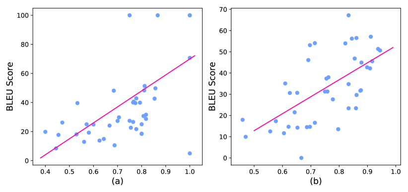
Figure 4: Performance (in BLEU) on the test set with respect to the node (a) and edge (b) prediction accuracy.

Setting	LDC2015E86	LDC2017T10
Node Prediction Acc.	0.65	0.71
Edge Prediction Acc.	0.56	0.59
Both Prediction Acc.	0.69	0.73

Table 6: The pearson correlation coefficient $\rho$ between the prediction accuracy and BLEU.

Correlation between Prediction Accuracy and Model Performance  We further investigate the influence of AMR-structure preservation on the performance of the main text generation task. Specifically, we first force our model to generate a gold sentence in order to calculate the accuracies for node prediction and edge prediction. We then calculate the corresponding BLEU score for the sentence generated by our model on the same input AMR graph without forced decoding, before drawing correlation between the accuracies and the BLEU score. As shown in Figure 4(a) and 4(b), both node accuracy and edge accuracy have a strong positive correlation with the BLEU score, indicating that the more structural information is retained, the better the generated text is.

We also evaluate the pearson ($\rho$) correlation coefficients between BLEU scores and node (edge) prediction accuracies. Results are given in Table 6. Both types of prediction accuracies have strong positive correlations with the final BLEU scores, and their combination yields further boost on the correlation coefficient, indicating the necessity of jointly predicting the nodes and edges.

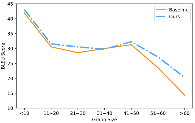
Figure 5: Performances (in BLEU) on the test set with respect to the size of the input AMR graphs.

Performances VS AMR Graphs Sizes Figure 5 compares the BLEU scores of the baseline and our model on different AMR sizes. Our model is consistently better than the baseline for most length brackets, and the advantage is more obvious for large AMRs (size 51+).

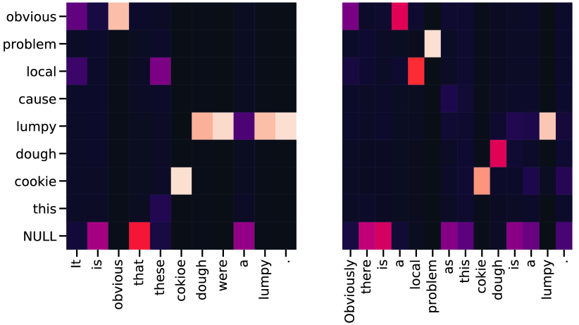
Figure 6: Visualization of word-to-node attention obtained from the baseline graph Transformer (left) and our model with node prediction loss (right).

4.5 Case Study

We provide two examples in Table 7 to help better understand the proposed model. Each example consists of an AMR graph, a reference sentence (REF), the output of baseline model (Baseline) and the sentence generated by our method (Ours).

As shown in the first example, although the baseline model maintains the main idea of the original text, it fails to recognize the AMR graph nodes “local” and “problem”. In contrast, our model successfully recovers these two nodes and generates a sentence which is more faithful to the reference. We attribute this improvement to node prediction. To verify this, we visualize the word-to-node attention scores of both approaches in Figure 6. As shown in the figure, the baseline model gives little attention to the AMR node “local” and “problem” during text generation. In contrast, our system gives a more accurate alignment to the relevant AMR nodes in decoding.

In the second example, the baseline model incorrectly positions the terms “doctor”, “see” and “worse cases” while our approach generates a more natural sentence. This can be attributed to the edge prediction task, which can inform the decoder to preserve the relation that “doctor” is the subject of “see” and “worse cases” is the object.

(1) (o / obvious-01

:ARG1 (p / problem

:ARG1-of (l / local-02))

:ARG1-of (c / cause-01

:ARG0 (l2 / lumpy

:domain (d / dough

:mod (c2 / cookie)

:mod (t / this)))))

REF: Obviously there are local problems because this

cookie dough is lumpy .

Baseline: It is obvious that these cookie dough were a

lumpy .

Ours: Obviously there is a local problem as this cookie

dough is a lumpy .

(2) (c / cause-01

:ARG0 (s / see-01

:ARG0 (d / doctor)

:ARG1 (c2 / case

:ARG1-of (b / bad-05

:degree (m / more

:quant (m2 / much)))))

:ARG1 (w / worry :polarity - :mode imperative

:ARG0 (y / you)

:ARG1 (t / that)))

REF: Doctors have seen much worse cases so don’t

worry about that !

Baseline: Don’t worry about that see much worse

cases by doctors .

Ours: Don’t worry that , as a doctor saw much worse

cases .

Table 7: Examples for case study.

5 Related Work

Early studies on AMR-to-text generation rely on statistical methods. Flanigan et al. (2016) convert input AMR graphs to trees by splitting re-entrances, before translating these trees into target sentences with a tree-to-string transducer; Pourdamghani et al. (2016) apply a phrase-based MT system on linearized AMRs; Song et al. (2017) design a synchronous node replacement grammar to parse input AMRs while generating target sentences. These approaches show comparable or better results than early neural models Konstas et al. (2017). However, recent neural approaches Song et al. (2018); Zhu et al. (2019); Cai and Lam (2020); Wang et al. (2020); Mager et al. (2020) have demonstrated the state-of-the-art performances thanks to the use of contextualized embeddings.

Related work on NMT studies back-translation loss Sennrich et al. (2016); Tu et al. (2017) by translating the target reference back into the source text (reconstruction), which can help retain more comprehensive input information. This is similar to our goal. Wiseman et al. (2017) extended the reconstruction loss of Tu et al. (2017) for table-to-text generation. We study a more challenging topic on how to retain the meaning of a complex graph structure rather than a sentence or a table. In addition, rather than reconstructing the input after the output is produced, we predict the input while the output is constructed, thereby allowing stronger information sharing.

Our work is also remotely related to previous work on string-to-tree neural machine translation (NMT) (Aharoni and Goldberg, 2017; Wu et al., 2017; Wang et al., 2018), which aims at generating target sentences together with their syntactic trees. One major difference is that their goal is producing grammatical outputs, while ours is preserving input structural information.

6 Conclusion

We investigated back-parsing for AMR-to-text generation by integrating the prediction of projected AMRs into sentence decoding. The resulting model benefits from both richer loss and more structual features during decoding. Experiments on two benchmarks show advantage of our model over a state-of-the-art baseline.

Appendix A Appendices

A.1 Full Experimental Settings

Parameter	Value	Parameter	Value
Src vocab (BPE)	10,004	Optimizer	Adam
Tgt vocab (BPE)	10,004	Learning rate	0.5
Relation vocab	5,002	Adam beta1	0.9
Encoder layer	6	Adam beta2	0.98
Decoder layer	6	Lr decay	0.5
Hidden size	512	Decay method	noam
Attention heads	8	Decay step	10,000
Attention dropout	0.3	Warmup	16,000
Share_embeddings	True	Batch size	2048
Python version	3.6	$\lambda_{1}$	0.01
Pytorch version	1.0.1	$\lambda_{2}$	0.1
Model parameters	67.93M	Training time	30h

Table 8: Full list of model parameters on the LDC2015E86.

Model	LDC2015E86			LDC2017T10
	BLEU	Meteor	CHRF++	BLEU	Meteor	CHRF++
LSTM Konstas et al. (2017)	22.00	-	-	-	-	-
GRN Song et al. (2018)	23.30	-	-	-	-	-
Syntax-G Cao and Clark (2019)	23.5	-	-	26.8	-	-
S-Enc Damonte and Cohen (2019)	24.40	23.60	-	24.54	24.07	-
DCGCN Guo et al. (2019)	25.9	-	-	27.9	-	57.3
G-Trans-F Zhu et al. (2019)	27.23	34.53	61.55	30.18	35.83	63.20
G-Trans-SA Zhu et al. (2019)	29.66	35.45	63.00	31.54	36.02	63.84
G-Trans-C Cai and Lam (2020)	27.4	32.9	56.4	29.8	35.1	59.4
G-Trans-W Wang et al. (2020)	25.9	-	-	29.3	-	59.0
G-Trans-F-Ours	30.15	35.36	63.08	31.93	37.23	64.20
+ Node Prediction	30.72	35.94	63.56	32.99	37.33	64.53
+ Edge Prediction	31.07	35.87	63.73	33.44	37.45	64.62
+ Both Prediction	31.48	36.15	63.87	34.19	38.18	65.72

Table 9: Main test results on LDC2015E86 and LDC2017T10.

Table 8 lists all model hyperparameters used for experiments. Specifically, we share the vocabulary of AMR node BPEs and target word BPEs. Our implementation is based on the model of Zhu et al. (2019), which is available at https://github.com/Amazing-J/structural-transformer. Our re-implementation and the proposed model are released at https://github.com/muyeby/AMR-Backparsing.

A.2 More Results

We compare our model with more baselines and use more evaluation metrics (BLEU Papineni et al. (2002), Meteor Banerjee and Lavie (2005); Denkowski and Lavie (2014) and CHRF++ Popović (2017)). The results are shown in Table 9. It can be observed that our approach achieves the best performance on both datasets regardless of the evaluation metrics. This observation is consistent with Table 2.

References

- Aharoni and Goldberg (2017) Roee Aharoni and Yoav Goldberg. 2017. Towards string-to-tree neural machine translation. In Proceedings of the 55th Annual Meeting of the Association for Computational Linguistics (Volume 2: Short Papers).
- Banarescu et al. (2013) Laura Banarescu, Claire Bonial, Shu Cai, Madalina Georgescu, Kira Griffitt, Ulf Hermjakob, Kevin Knight, Philipp Koehn, Martha Palmer, and Nathan Schneider. 2013. Abstract meaning representation for sembanking. In Proceedings of the 7th Linguistic Annotation Workshop and Interoperability with Discourse.
- Banerjee and Lavie (2005) Satanjeev Banerjee and Alon Lavie. 2005. METEOR: An automatic metric for MT evaluation with improved correlation with human judgments. In Proceedings of the ACL Workshop on Intrinsic and Extrinsic Evaluation Measures for Machine Translation and/or Summarization, pages 65–72, Ann Arbor, Michigan. Association for Computational Linguistics.
- Beck et al. (2018) Daniel Beck, Gholamreza Haffari, and Trevor Cohn. 2018. Graph-to-sequence learning using gated graph neural networks. In Proceedings of the 56th Annual Meeting of the Association for Computational Linguistics (Volume 1: Long Papers).
- Belz et al. (2011) Anja Belz, Michael White, Dominic Espinosa, Eric Kow, Deirdre Hogan, and Amanda Stent. 2011. The first surface realisation shared task: Overview and evaluation results. In Proceedings of the 13th European workshop on natural language generation, pages 217–226. Association for Computational Linguistics.
- Cai and Lam (2020) Deng Cai and Wai Lam. 2020. Graph transformer for graph-to-sequence learning. In Proceedings of Thirty-Fourth AAAI Conference on Artificial Intelligence.
- Cao and Clark (2019) Kris Cao and Stephen Clark. 2019. Factorising AMR generation through syntax. In Proceedings of the 2019 Conference of the North American Chapter of the Association for Computational Linguistics: Human Language Technologies, Volume 1 (Long and Short Papers), pages 2157–2163, Minneapolis, Minnesota. Association for Computational Linguistics.
- Damonte and Cohen (2019) Marco Damonte and Shay B Cohen. 2019. Structural neural encoders for amr-to-text generation. In Proceedings of the 2019 Conference of the North American Chapter of the Association for Computational Linguistics: Human Language Technologies, Volume 1 (Long and Short Papers).
- Denkowski and Lavie (2014) Michael Denkowski and Alon Lavie. 2014. Meteor universal: Language specific translation evaluation for any target language. In Proceedings of the Ninth Workshop on Statistical Machine Translation, pages 376–380, Baltimore, Maryland, USA. Association for Computational Linguistics.
- Dozat and Manning (2016) Timothy Dozat and Christopher D Manning. 2016. Deep biaffine attention for neural dependency parsing. In International Conference on Learning Representations.
- Flanigan et al. (2016) Jeffrey Flanigan, Chris Dyer, Noah A Smith, and Jaime G Carbonell. 2016. Generation from abstract meaning representation using tree transducers. In Proceedings of the 2016 Conference of the North American Chapter of the Association for Computational Linguistics: Human Language Technologies.
- Gardent et al. (2017) Claire Gardent, Anastasia Shimorina, Shashi Narayan, and Laura Perez-Beltrachini. 2017. The webnlg challenge: Generating text from rdf data. In Proceedings of the 10th International Conference on Natural Language Generation, pages 124–133.
- Guo et al. (2019) Zhijiang Guo, Yan Zhang, Zhiyang Teng, and Wei Lu. 2019. Densely connected graph convolutional networks for graph-to-sequence learning. Transactions of the Association for Computational Linguistics, 7:297–312.
- Hajdik et al. (2019) Valerie Hajdik, Jan Buys, Michael Wayne Goodman, and Emily M Bender. 2019. Neural text generation from rich semantic representations. In Proceedings of the 2019 Conference of the North American Chapter of the Association for Computational Linguistics: Human Language Technologies, Volume 1 (Long and Short Papers).
- Hardy and Vlachos (2018) Hardy Hardy and Andreas Vlachos. 2018. Guided neural language generation for abstractive summarization using abstract meaning representation. In Proceedings of the 2018 Conference on Empirical Methods in Natural Language Processing.
- Kingma and Ba (2015) Diederik P. Kingma and Jimmy Ba. 2015. Adam: A method for stochastic optimization. In International Conference for Learning Representations.
- Koncel-Kedziorski et al. (2019) Rik Koncel-Kedziorski, Dhanush Bekal, Yi Luan, Mirella Lapata, and Hannaneh Hajishirzi. 2019. Text generation from knowledge graphs with graph transformers. In Proceedings of the 2019 Conference of the North American Chapter of the Association for Computational Linguistics: Human Language Technologies, Volume 1 (Long and Short Papers).
- Konstas et al. (2017) Ioannis Konstas, Srinivasan Iyer, Mark Yatskar, Yejin Choi, and Luke Zettlemoyer. 2017. Neural amr: Sequence-to-sequence models for parsing and generation. In Proceedings of the 55th Annual Meeting of the Association for Computational Linguistics (Volume 1: Long Papers).
- Liao et al. (2018) Kexin Liao, Logan Lebanoff, and Fei Liu. 2018. Abstract meaning representation for multi-document summarization. In Proceedings of the 27th International Conference on Computational Linguistics.
- Liu et al. (2015) Fei Liu, Jeffrey Flanigan, Sam Thomson, Norman Sadeh, and Noah A Smith. 2015. Toward abstractive summarization using semantic representations. In Proceedings of the 2015 Conference of the North American Chapter of the Association for Computational Linguistics: Human Language Technologies.
- Liu et al. (2016) Lemao Liu, Masao Utiyama, Andrew Finch, and Eiichiro Sumita. 2016. Neural machine translation with supervised attention. In Proceedings of COLING 2016, the 26th International Conference on Computational Linguistics: Technical Papers.
- Mager et al. (2020) Manuel Mager, Ramón Fernandez Astudillo, Tahira Naseem, Md Arafat Sultan, Young-Suk Lee, Radu Florian, and Salim Roukos. 2020. GPT-too: A language-model-first approach for AMR-to-text generation. In Proceedings of the 58th Annual Meeting of the Association for Computational Linguistics, pages 1846–1852, Online. Association for Computational Linguistics.
- Mi et al. (2016) Haitao Mi, Zhiguo Wang, and Abe Ittycheriah. 2016. Supervised attentions for neural machine translation. In Proceedings of the 2016 Conference on Empirical Methods in Natural Language Processing.
- Papineni et al. (2002) Kishore Papineni, Salim Roukos, Todd Ward, and Wei-Jing Zhu. 2002. Bleu: a method for automatic evaluation of machine translation. In Proceedings of the 40th Annual Meeting of the Association for Computational Linguistics.
- Popović (2017) Maja Popović. 2017. chrF++: words helping character n-grams. In Proceedings of the Second Conference on Machine Translation.
- Pourdamghani et al. (2014) Nima Pourdamghani, Yang Gao, Ulf Hermjakob, and Kevin Knight. 2014. Aligning English strings with abstract meaning representation graphs. In Proceedings of the 2014 Conference on Empirical Methods in Natural Language Processing (EMNLP).
- Pourdamghani et al. (2016) Nima Pourdamghani, Kevin Knight, and Ulf Hermjakob. 2016. Generating english from abstract meaning representations. In Proceedings of the 9th international natural language generation conference.
- Prasad et al. (2008) Rashmi Prasad, Nikhil Dinesh, Alan Lee, Eleni Miltsakaki, Livio Robaldo, Aravind Joshi, and Bonnie Webber. 2008. The Penn discourse TreeBank 2.0. In Proceedings of the Sixth International Conference on Language Resources and Evaluation (LREC’08), Marrakech, Morocco. European Language Resources Association (ELRA).
- Ribeiro et al. (2019) Leonardo FR Ribeiro, Claire Gardent, and Iryna Gurevych. 2019. Enhancing amr-to-text generation with dual graph representations. In Proceedings of the 2019 Conference on Empirical Methods in Natural Language Processing and the 9th International Joint Conference on Natural Language Processing (EMNLP-IJCNLP).
- Sennrich et al. (2016) Rico Sennrich, Barry Haddow, and Alexandra Birch. 2016. Improving neural machine translation models with monolingual data. In Proceedings of the 54th Annual Meeting of the Association for Computational Linguistics (Volume 1: Long Papers).
- Song et al. (2019) Linfeng Song, Daniel Gildea, Yue Zhang, Zhiguo Wang, and Jinsong Su. 2019. Semantic neural machine translation using amr. Transactions of the Association for Computational Linguistics, 7:19–31.
- Song et al. (2017) Linfeng Song, Xiaochang Peng, Yue Zhang, Zhiguo Wang, and Daniel Gildea. 2017. Amr-to-text generation with synchronous node replacement grammar. In Proceedings of the 55th Annual Meeting of the Association for Computational Linguistics (Volume 2: Short Papers).
- Song et al. (2018) Linfeng Song, Yue Zhang, Zhiguo Wang, and Daniel Gildea. 2018. A graph-to-sequence model for amr-to-text generation. In Proceedings of the 56th Annual Meeting of the Association for Computational Linguistics (Volume 1: Long Papers).
- Tu et al. (2017) Zhaopeng Tu, Yang Liu, Lifeng Shang, Xiaohua Liu, and Hang Li. 2017. Neural machine translation with reconstruction. In Thirty-First AAAI Conference on Artificial Intelligence.
- Vaswani et al. (2017) Ashish Vaswani, Noam Shazeer, Niki Parmar, Jakob Uszkoreit, Llion Jones, Aidan N Gomez, Łukasz Kaiser, and Illia Polosukhin. 2017. Attention is all you need. In Advances in neural information processing systems.
- Wang et al. (2020) Tianming Wang, Xiaojun Wan, and Hanqi Jin. 2020. Amr-to-text generation with graph transformer. Transactions of the Association for Computational Linguistics, 8:19–33.
- Wang et al. (2018) Xinyi Wang, Hieu Pham, Pengcheng Yin, and Graham Neubig. 2018. A tree-based decoder for neural machine translation. In Proceedings of the 2018 Conference on Empirical Methods in Natural Language Processing.
- Wiseman et al. (2017) Sam Wiseman, Stuart M Shieber, and Alexander M Rush. 2017. Challenges in data-to-document generation. In Proceedings of the 2017 Conference on Empirical Methods in Natural Language Processing.
- Wu et al. (2017) Shuangzhi Wu, Dongdong Zhang, Nan Yang, Mu Li, and Ming Zhou. 2017. Sequence-to-dependency neural machine translation. In Proceedings of the 55th Annual Meeting of the Association for Computational Linguistics (Volume 1: Long Papers).
- Yasunaga et al. (2017) Michihiro Yasunaga, Rui Zhang, Kshitijh Meelu, Ayush Pareek, Krishnan Srinivasan, and Dragomir Radev. 2017. Graph-based neural multi-document summarization. In Proceedings of the 21st Conference on Computational Natural Language Learning (CoNLL 2017).
- Zhang et al. (2020) Tianyi Zhang, Varsha Kishore, Felix Wu, Kilian Q. Weinberger, and Yoav Artzi. 2020. Bertscore: Evaluating text generation with bert. In International Conference on Learning Representations.
- Zhu et al. (2019) Jie Zhu, Junhui Li, Muhua Zhu, Longhua Qian, Min Zhang, and Guodong Zhou. 2019. Modeling graph structure in transformer for better amr-to-text generation. In Proceedings of the 2019 Conference on Empirical Methods in Natural Language Processing and the 9th International Joint Conference on Natural Language Processing (EMNLP-IJCNLP).
- Çelikyilmaz et al. (2020) A. Çelikyilmaz, Elizabeth Clark, and Jianfeng Gao. 2020. Evaluation of text generation: A survey. ArXiv, abs/2006.14799.