Autoregressive Networks

Abstract

We propose a first-order autoregressive (i.e. AR(1)) model for dynamic network processes in which edges change over time while nodes remain unchanged. The model depicts the dynamic changes explicitly. It also facilitates simple and efficient statistical inference methods including a permutation test for diagnostic checking for the fitted network models. The proposed model can be applied to the network processes with various underlying structures but with independent edges. As an illustration, an AR(1) stochastic block model has been investigated in depth, which characterizes the latent communities by the transition probabilities over time. This leads to a new and more effective spectral clustering algorithm for identifying the latent communities. We have derived a finite sample condition under which the perfect recovery of the community structure can be achieved by the newly defined spectral clustering algorithm. Furthermore the inference for a change point is incorporated into the AR(1) stochastic block model to cater for possible structure changes. We have derived the explicit error rates for the maximum likelihood estimator of the change-point. Application with three real data sets illustrates both relevance and usefulness of the proposed AR(1) models and the associate inference methods.

Keywords: AR(1) networks; Change point; Dynamic stochastic block model; Hamming distance; Maximum likelihood estimation; Spectral clustering algorithm; Yule-Walker equation.

1 Introduction

Understanding and being able to model the network changes over time are of immense importance for, e.g., monitoring anomalies in internet traffic networks, predicting demand and setting prices in electricity supply networks, managing natural resources in environmental readings in sensor networks, and understanding how news and opinion propagates in online social networks. In spite of the existence of a large body of literature on dynamic networks, the development of the foundation for dynamic network models is still in its infancy (Kolaczyk,, 2017). As for dealing with dynamic changes of networks, early attempts are based on the evolution analysis of network snapshots over time (Aggarwal and Subbian,, 2014; Donnat and Holmes,, 2018). Although this reflects the fact that most networks change slowly over time, it provides little insight on the dynamics underlying the changes and is almost powerless for future prediction. The popular approaches for modelling dynamic changes include, among others, Markov process models (Snijders,, 2005; Ludkin et al.,, 2018), the exponential random graph models (Hanneke et al.,, 2010; Krivitsky and Handcock,, 2014), and latent process based models (Friel et al.,, 2016; Durante et al.,, 2016; Matias and Miele,, 2017). The estimation for those models is compute-intensive, relying on various MCMC or EM algorithms.

In this paper we propose a simple first-order autoregressive (i.e. AR(1)) model for dynamic network processes of which the edges changes over time while the nodes are unchanged. Though our setting is a special case of the Markov chain network models (see Yudovina et al., (2015), and also Snijders, (2005) and Ludkin et al., (2018)), a simple AR(1) structure makes it possible to measure explicitly the underlying dynamic properties such as autocorrelation coefficients, and the Hamming distance. It facilitates the maximum likelihood estimation (MLE) in a simple and direct manner with uniform error rates. Furthermore diagnostic checking for the fitted network models can be performed in terms of an easy-to-use permutation test, which is impossible under a merely Markovian structure.

Our setting can be applied to any network processes with various underlying structures as long as the edges are independent with each other, which we illustrate through an AR(1) stochastic block model. The latent communities in our setting are characterized by the transition probabilities over time, instead of the (static) connection probabilities – the approach often adopted from static stochastic block models; see Pensky, (2019) and the references therein. This new structure also paves the way for a new spectral clustering algorithm which identifies the latent communities more effectively – a phenomenon corroborated by both the asymptotic theory and the simulation results. To cater for possible structure changes of underlying processes, we incorporate a change point detection mechanism in the AR(1) stochastic block modeling. Again the change point is estimated by the maximum likelihood method. The AR(1) continuous time stochastic block model of Ludkin et al., (2018) is based on a sophisticated construction. Its estimation is based on a reversible jump MCMC, though a discrete-time version of their model admits the same Markov Chain representation (2.3) below.

Theoretical developments for dynamic stochastic block models in the literature were typically based on the assumption that networks observed at different times are independent; see Pensky, (2019); Bhattacharjee et al., (2020) and references therein. The autoregressive structure considered in this paper brings the extra complexity due to serial dependence. By establishing the $\alpha$-mixing property with exponentially decaying coefficients for the AR(1) network processes, we are able to show that the proposed spectral clustering algorithm leads to a consistent recovery of the latent community structure. On the other hand, an extra challenge in detecting a change point in the dynamic stochastic block network process is that the estimation for latent community structures before and after a possible change point is typically not consistent during the search for the change point. To overcome this obstacle, we introduce a truncation technique which breaks the searching interval into two parts such that the error bounds for the estimated change point can be established.

The proposed methods in this paper only apply to the dynamic networks observed on discrete times. Even so the relevant literature is large, across mathematics, computer science, engineer, statistics, biology, genetics and social sciences. We can only list a small selection of more statistics-oriented papers in addition to the aforementioned references. Fu et al., (2009) proposed a state space mixed membership stochastic block model (with a logistic normal prior). Crane et al., (2016) studied the limit properties of Markovian, exchangeable and càdlàg (i.e. every edge remains in each state which it visits for a positive amount of time) dynamic network. Pensky, (2019) studied the theoretical properties (such as the minimax lower bounds for the risk) of a dynamic stochastic block model, assuming ‘smooth’ connectivity probabilities. The literature on change point detection in dynamic networks includes Yang et al., (2011); Wang et al., (2018); Wilson et al., (2019); Zhao et al., (2019); Bhattacharjee et al., (2020); Zhu et al., 2020a . Knight et al., (2016); Zhu et al., (2017, 2019); Chen et al., (2020); Zhu et al., 2020b adopted autoregressive models for modelling continuous responses observed from the nodes of a network process. Kang et al., (2017) used dynamic network as a tool to model non-stationary vector autoregressive processes. For the development on continuous-time dynamic networks, we refer readers to Snijders, (2005), Matias et al., (2018), Ludkin et al., (2018) and Corneli et al., (2018).

The new contributions of this paper include: (i) We propose a new and simple AR(1) model for edge dymanics (see (2.1) below), which facilitates the easy-to-use inference methods including a permutation test for model diagnostic checking. (ii) The AR(1) setting can be applied to various network processes with specific underlying structures such as dynamic stochastic block models, as illustrated in Section 3 below, and also dynamic dot product model, dynamic graphon model, etc. (iii) The AR(1) structure also makes it possible to develop the theoretical guarantees for the serial dependent network processes. For example, based on a concentration inequality, we have derived a finite sample condition, under which the perfect recovery of the community structure can be achieved by the newly defined spectral clustering algorithm (Theorems 1 and 2 in Section 3.2.2 below). Furthermore, we have shown that the MLE for the change-point in the AR(1) stochastic block process is consistent with explicit error rates (Theorem 5 in Section 3.3 below). Those results are based on some rigorous technical development for the dependent network processes. Note that both Pensky, (2019) and Bhattacharjee et al., (2020) assume that networks observed at different times are independent with each other in their asymptotic theories for dynamic stochastic block models. Illustration with the three real network data sets indicates convincingly that the proposed AR(1) model and the associated inference methods are practically relevant and fruitful.

The rest of the paper is organized as follows. A general framework of AR(1) network processes, the probabilistic properties, and the MLE are presented in Section 2. It also contains a new and easy-to-use permutation test for the diagnostic checking for the fitted network models. Section 3 deals with AR(1) stochastic block models. The asymptotic theory is developed for the new spectral clustering algorithm based on the transition probabilities. Further extension of both the inference method and the asymptotic theory to the setting with a change point is established. Simulation results are reported in Section 4, and the illustration with three real dynamic network data sets is presented in Section 5. All technical proofs are relegated to the Appendix.

2 Autoregressive network models

2.1 AR(1) models

Let $\{{\mathbf{X}}_{t},t=0,1,2,\cdots\}$ be a dynamic network process defined on the $p$ fixed nodes, denoted by $\{1,\cdots,p\}$, where ${\mathbf{X}}_{t}\equiv(X_{i,j}^{t})$ denotes the $p\times p$ adjacency matrix at time $t$. We also assume that all networks are Erdös-Renyi in the sense that $X_{i,j}^{t}$, $(i,j)\in{\mathcal{J}}$, are independent and take values either 1 or 0, where ${\mathcal{J}}=\{(i,j):1\leq i\leq j\leq p\}$ for undirected networks, ${\mathcal{J}}=\{(i,j):1\leq i<j\leq p\}$ for undirected networks without selfloops, ${\mathcal{J}}=\{(i,j):1\leq i,j\leq p\}$ for directed networks, and ${\mathcal{J}}=\{(i,j):1\leq i\neq j\leq p\}$ for directed networks without selfloops. Note that an edge from node $i$ to $j$ is indicated by $X_{i,j}=1$, and no edge is denoted by $X_{i,j}=0$. For undirected networks, $X_{i,j}^{t}=X_{j,i}^{t}$.

Definition 2.1.

An AR(1) network process is defined as

$$X^{t}_{i,j}\;=\;X^{t-1}_{i,j}\,I({\varepsilon}_{i,j}^{t}=0)\;+\;I({\varepsilon}_{i,j}^{t}=1),\quad t\geq 1,$$ (2.1)

where $I(\cdot)$ denotes the indicator function, the innovations ${\varepsilon}_{i,j}^{t}$, $(i,j)\in{\mathcal{J}}$, are independent, and

$$P({\varepsilon}_{i,j}^{t}=1)=\alpha_{i,j}^{t},\quad P({\varepsilon}_{i,j}^{t}=-1)=\beta_{i,j}^{t},\quad P({\varepsilon}_{i,j}^{t}=0)=1-\alpha_{i,j}^{t}-\beta_{i,j}^{t}.$$ (2.2)

In the above expression, $\alpha_{i,j}^{t},\beta_{i,j}^{t}$ are non-negative constants, and $\alpha_{i,j}^{t}+\beta_{i,j}^{t}\leq 1$.

Equation (2.1) is an analogue of the noisy network model of Chang et al., 2020c . The innovation (or noise) ${\varepsilon}_{i,j}^{t}$ is ‘added’ via the two indicator functions to ensure that $X_{i,j}^{t}$ is still binary. Obviously, $\{{\mathbf{X}}_{t},t=0,1,2,\cdots\}$ is a Markov chain, and

$$P(X_{i,j}^{t}=1|X_{i,j}^{t-1}=0)=\alpha_{i,j}^{t},\quad P(X_{i,j}^{t}=0|X_{i,j}^{t-1}=1)=\beta_{i,j}^{t},$$ (2.3)

or collectively,

$$P({\mathbf{X}}_{t}|{\mathbf{X}}_{t-1},\cdots,{\mathbf{X}}_{0})\;=\;P({\mathbf{X}}_{t}|{\mathbf{X}}_{t-1})\;=\;\prod_{(i,j)\in{\mathcal{J}}}P(X_{i,j}^{t}|X_{i,j}^{t-1})$$ (2.4)

$$=\; \prod_{(i,j)\in{\mathcal{J}}}(\alpha_{i,j}^{t})^{X_{i,j}^{t}(1-X_{i,j}^{t-1})}(1-\alpha_{i,j}^{t})^{(1-X_{i,j}^{t})(1-X_{i,j}^{t-1})}(\beta_{i,j}^{t})^{(1-X_{i,j}^{t})X_{i,j}^{t-1}}(1-\beta_{i,j}^{t})^{X_{i,j}^{t}X_{i,j}^{t-1}}.$$

It is clear that the smaller $\alpha_{i,j}^{t}$ is, the more likely the no-edge status at time $t-1$ (i.e. $X_{i,j}^{t-1}=0$) will be retained at time $t$ (i.e. $X_{i,j}^{t}=0$); and the smaller $\beta_{i,j}^{t}$ is, the more likely an edge at time $t-1$ (i.e. $X_{i,j}^{t-1}=1$) will be retained at time $t$ (i.e. $X_{i,j}^{t}=1$). For most slowly changing networks (such as social networks), we expect $\alpha_{i,j}^{t}$ and $\beta_{i,j}^{t}$ to be small.

It is natural to model dynamic networks by a Markov chain. See, e.g. Hanneke et al., (2010); Krivitsky and Handcock, (2014); Yudovina et al., (2015); Friel et al., (2016); Crane et al., (2016); Matias and Miele, (2017); Rastelli et al., (2017); Ludkin et al., (2018). For example, the Markovian transition probabilities under a discrete version of the stationary independent arcs network model of Snijders (2005, Section 5) can be written equivalently as (2.3) with $\alpha^{t}_{i,j}\equiv\alpha$ and $\beta^{t}_{i,j}\equiv\beta$. In this paper we build the Markovian structure based on the explicit AR(1) model (2.1), which enables us to study the theoretical properties of the network processes, and to develop simple and efficient inference methods with appropriate theoretical guarantee.

2.2 Stationarity

Note that $\{{\mathbf{X}}_{t}\}$ is a homogeneous Markov chain if

$$\alpha_{i,j}^{t}\equiv\alpha_{i,j}\quad{\rm and}\quad\beta_{i,j}^{t}\equiv\beta_{i,j}\;\;\;{\rm for\;all\;}t\geq 1\;\;{\rm and}\;\;(i,j)\in{\mathcal{J}}.$$ (2.5)

Specify the distribution of the initial network ${\mathbf{X}}_{0}=(X_{i,j}^{0})$ as follows:

$$P(X_{i,j}^{0}=1)=\pi_{i,j}=1-P(X_{i,j}^{0}=0),$$ (2.6)

where $\pi_{i,j}\in(0,1)$, $(i,j)\in{\mathcal{J}}$, are constants.

Proposition 1.

Let the homogeneity condition (2.5) hold with $\alpha_{i,j}+\beta_{i,j}\in(0,1]$, and

$$\pi_{i,j}=\alpha_{i,j}/(\alpha_{i,j}+\beta_{i,j}),\;\;(i,j)\in{\mathcal{J}}.$$ (2.7)

Then $\{{\mathbf{X}}_{t},t=0,1,2,\cdots\}$ is a strictly stationary process. Furthermore for any $(i,j),(\ell,m)\in{\mathcal{J}}$ and $t,s\geq 0$,

$$E(X_{i,j}^{t})={\alpha_{i,j}\over\alpha_{i,j}+\beta_{i,j}},\qquad{\rm Var}(X_{i,j}^{t})={\alpha_{i,j}\beta_{i,j}\over(\alpha_{i,j}+\beta_{i,j})^{2}},$$ (2.8)

$$\rho_{i,j}(|t-s|)\equiv{\rm Corr}(X_{i,j}^{t},X_{\ell m}^{s})=\Big{\{}\begin{array}[]{ll}(1-\alpha_{i,j}-\beta_{i,j})^{|t-s|}&{\rm if}\;(i,j)=(\ell,m),\\ 0&{\rm otherwise}.\end{array}$$ (2.9)

The Hamming distance counts the number of different edges in the two networks, and is a measure the closeness of two networks (Donnat and Holmes,, 2018).

Definition 2.2.

For any two matrices ${\mathbf{A}}=(A_{i,j})$ and ${\mathbf{B}}=(B_{i,j})$ of the same size, the Hamming distance is defined as $D_{H}({\mathbf{A}},{\mathbf{B}})\;=\;\sum_{i,j}I(A_{i,j}\neq B_{i,j}).$

Proposition 2.

Let $\{{\mathbf{X}}_{t},t=0,1,\cdots\}$ be a stationary network process satisfying the condition of Proposition 1. Let $d_{H}(|t-s|)=E\{D_{H}({\mathbf{X}}_{t},{\mathbf{X}}_{s})\}$ for any $t,s\geq 0$. Then $d_{H}(0)=0$, and it holds for any $k\geq 1$ that

$$d_{H}(k) \;=\;d_{H}(k-1)+\sum_{(i,j)\in{\mathcal{J}}}{2\alpha_{i,j}\beta_{i,j}\over\alpha_{i,j}+\beta_{i,j}}(1-\alpha_{i,j}-\beta_{i,j})^{k-1}$$ (2.10)

$$\;=\sum_{(i,j)\in{\mathcal{J}}}{2\alpha_{i,j}\beta_{i,j}\over(\alpha_{i,j}+\beta_{i,j})^{2}}\{1-(1-\alpha_{i,j}-\beta_{i,j})^{k}\}.$$ (2.11)

Proposition 2 indicates that the expected Hamming distance $d_{H}(d)=E\{D_{H}({\mathbf{X}}_{t},{\mathbf{X}}_{t+k})\}$ increases strictly, as $k$ increases, initially from $d_{H}(1)=\sum{2\alpha_{i,j}\beta_{i,j}\over\alpha_{i,j}+\beta_{i,j}}$ towards the limit $d_{H}(\infty)=\sum{2\alpha_{i,j}\beta_{i,j}\over(\alpha_{i,j}+\beta_{i,j})^{2}}$ which is also the expected Hamming distance of the two independent networks sharing the same marginal distribution of ${\mathbf{X}}_{t}$.

Proposition 3 below shows that $\{{\mathbf{X}}_{t},\,t=0,1,\cdots\}$ is $\alpha$-mixing with exponentially decaying coefficients. Note that the conventional mixing results for ARMA processes do not apply here, as they typically require that the innovation distribution is continuous; see, e.g., Section 2.6.1 of Fan and Yao, (2003). Let ${\mathcal{F}}_{a}^{b}$ be the $\sigma$-algebra generated by $\{X_{i,j}^{k},a\leq k\leq b\}$. The $\alpha$-mixing coefficient of process $\{X_{i,j}^{t},t=0,1,\cdots\}$ is defined as

$$\alpha^{i,j}(\tau)=\sup_{k\in{\mathbb{N}}}\sup_{A\in{\mathcal{F}}_{0}^{k},B\in{\mathcal{F}}_{k+\tau}^{\infty},}|P(A\cap B)-P(A)P(B)|.$$

Proposition 3.

Let condition (2.5) hold, $\alpha_{i,j},\beta_{i,j}>0$, and $\alpha_{i,j}+\beta_{i,j}\leq 1$. Then $\alpha^{i,j}(\tau)\leq\rho_{i,j}(\tau)=(1-\alpha_{i,j}-\beta_{i,j})^{\tau}$ for any $\tau\geq 1$.

2.3 Estimation

To simplify the notation, we assume the availability of the observations ${\mathbf{X}}_{0},{\mathbf{X}}_{1},\cdots,{\mathbf{X}}_{n}$ from a stationary network process which satisfies the condition of Proposition 1. Without imposing any further structure on the model, the parameters $(\alpha_{i,j},\beta_{i,j})$, for different $(i,j)$, can be estimated separately. Condition on ${\mathbf{X}}_{0}$, the maximum likelihood estimators are

$$\widehat{\alpha}_{i,j}={\sum_{t=1}^{n}X^{t}_{i,j}(1-X_{i,j}^{t-1})\over\sum_{t=1}^{n}(1-X_{i,j}^{t-1})},\qquad\widehat{\beta}_{i,j}={\sum_{t=1}^{n}(1-X_{i,j}^{t})X_{i,j}^{t-1}\over\sum_{t=1}^{n}X_{i,j}^{t-1}}.$$ (2.12)

See (2.4). For definiteness we shall set $0/0=1$. To state the asymptotic properties, we list some regularity conditions first.

• There exists a constant $l>0$ such that $\alpha_{i,j},\beta_{i,j}\geq l$ and $\alpha_{i,j}+\beta_{i,j}\leq 1$ for all $(i,j)\in{\mathcal{J}}$.

• $n,p\rightarrow\infty$, and $(\log n)(\log\log n)\sqrt{\frac{\log p}{n}}\rightarrow 0$.

Condition C1 defines the parameter space, and condition C2 indicates that the number of nodes is allowed to diverge in a smaller order than $\exp\big{\{}\frac{n}{(\log n)^{2}(\log\log n)^{2}}\big{\}}$.

Proposition 4.

Let conditions (2.5), C1 and C2 hold. Then it holds that

$$\max_{(i,j)\in{\mathcal{J}}}|\widehat{\alpha}_{i,j}-\alpha_{i,j}|=O_{p}\left(\sqrt{\frac{\log p}{n}}\right)~{}~{}{\rm and}~{}~{}\max_{(i,j)\in{\mathcal{J}}}|\widehat{\beta}_{i,j}-\beta_{i,j}|=O_{p}\left(\sqrt{\frac{\log p}{n}}\right).$$

Proposition 4 provides a uniform convergence rate for the MLEs in (2.12). To state the joint asymptotic normality. Let ${J}_{1}=\{(i_{1},j_{1}),\ldots,(i_{m_{1}},j_{m_{1}})\}$, ${J}_{2}=\{(k_{1},\ell_{1}),\ldots,(k_{m_{2}},\ell_{m_{2}})\}$ be two arbitrary subsets of ${\mathcal{J}}$ with $m_{1},m_{2}\geq 1$ fixed. Denote $\boldsymbol{\Theta}_{J_{1},J_{2}}=(\alpha_{i_{1},j_{1}},\ldots,\alpha_{i_{m_{1}},j_{m_{1}}},$ $\beta_{k_{1},\ell_{1}},\ldots,\beta_{k_{m_{2}},\ell_{m_{2}}})^{\top},$ and correspondingly denote the MLEs as $\widehat{\boldsymbol{\Theta}}_{J_{1},J_{2}}=(\widehat{\alpha}_{i_{1},j_{1}},\ldots,\widehat{\alpha}_{i_{m_{1}},j_{m_{1}}},$ $\widehat{\beta}_{k_{1},\ell_{1}},\ldots,\widehat{\beta}_{k_{m_{2}},\ell_{m_{2}}})^{\top}$.

Proposition 5.

Let conditions (2.5), C1 and C2 hold. Then $\sqrt{n}(\widehat{\boldsymbol{\Theta}}_{J_{1},J_{2}}-\boldsymbol{\Theta}_{J_{1},J_{2}})\rightarrow N({\bf 0},\boldsymbol{\Sigma}_{J_{1},J_{2}}),$ where $\boldsymbol{\Sigma}_{J_{1},J_{2}}={\rm diag}(\sigma_{11},\ldots,\sigma_{m_{1}+m_{2},m_{1}+m_{2}})$ is a diagonal matrix with

$$\sigma_{rr}=\frac{\alpha_{i_{r},j_{r}}(1-\alpha_{i_{r},j_{r}})(\alpha_{i_{r},j_{r}}+\beta_{i_{r},j_{r}})}{\beta_{i_{r},j_{r}}},~{}~{}1\leq r\leq m_{1},$$

$$\sigma_{rr}=\frac{\beta_{k_{r},\ell_{r}}(1-\beta_{k_{r},\ell_{r}})(\alpha_{k_{r},\ell_{r}}+\beta_{k_{r},\ell_{r}})}{\alpha_{k_{r},\ell_{r}}},~{}~{}m_{1}+1\leq r\leq m_{1}+m_{2}.$$

2.4 Model diagnostic check

Based on estimators in (2.12), we define ‘residual’ $\widehat{\varepsilon}_{i,j}^{t}$, resulted from fitting model (2.1) to the data, as the estimated value of $E({\varepsilon}_{i,j}^{t}|X^{t}_{i,j},X^{t-1}_{i,j})$, i.e.

$$\widehat{\varepsilon}_{i,j}^{t}= {\widehat{\alpha}_{i,j}\over 1-\widehat{\beta}_{i,j}}I(X^{t}_{i,j}=1,X^{t-1}_{i,j}=1)-{\widehat{\beta}_{i,j}\over 1-\widehat{\alpha}_{i,j}}I(X^{t}_{i,j}=0,X^{t-1}_{i,j}=0)$$

$$+ I(X^{t}_{i,j}=1,X^{t-1}_{i,j}=0)-I(X^{t}_{i,j}=0,X^{t-1}_{i,j}=1),\quad(i,j)\in{\mathcal{J}},\;t=1,\cdots,n.$$

One way to check the adequacy of the model is to test for the independence of $\widehat{\EuScriptBF}E_{t}\equiv(\widehat{\varepsilon}_{i,j}^{t})$ for $t=1,\cdots,n$. Since $\widehat{\varepsilon}_{i,j}^{t}$, $t=1,\cdots,n$, only take 4 different values for each $(i,j)\in{\mathcal{J}}$, we adopt the two-way, or three-way contingency table to test the independence of $\widehat{\EuScriptBF}E_{t}$ and $\widehat{\EuScriptBF}E_{t-1}$, or $\widehat{\EuScriptBF}E_{t},\widehat{\EuScriptBF}E_{t-1}$ and $\widehat{\EuScriptBF}E_{t-2}$. For example the test statistic for the two-way contingency table is

$$T={1\over n\,|{\mathcal{J}}|}\sum_{(i,j)\in{\mathcal{J}}}\sum_{k,\ell=1}^{4}\{n_{i,j}(k,\ell)-n_{i,j}(k,\cdot)n_{i,j}(\cdot,\ell)/(n-1)\}^{2}\big{/}\{n_{i,j}(k,\cdot)n_{i,j}(\cdot,\ell)/(n-1)\},$$ (2.13)

where $|{\mathcal{J}}|$ denotes the cardinality of ${\mathcal{J}}$, and for $1\leq k,\ell\leq 4,$

$$n_{i,j}(k,\ell) =\sum_{t=2}^{n}I\{\widehat{\varepsilon}_{i,j}^{t}=u_{i,j}(k),\;\widehat{\varepsilon}_{i,j}^{t-1}=u_{i,j}(\ell)\},$$

$$n_{i,j}(k,\cdot) =\sum_{t=2}^{n}I\{\widehat{\varepsilon}_{i,j}^{t}=u_{i,j}(k)\},\quad n_{i,j}(\cdot,\ell)=\sum_{t=2}^{n}I\{\widehat{\varepsilon}_{i,j}^{t-1}=u_{i,j}(\ell)\}.$$

In the above expressions, $u_{i,j}(1)=-1,u_{i,j}(2)=-{\widehat{\beta}_{i,j}\over 1-\widehat{\alpha}_{i,j}},u_{i,j}(3)={\widehat{\alpha}_{i,j}\over 1-\widehat{\beta}_{i,j}}$ and $u_{i,j}(4)=1$. We calculate the $P$-values of the test $T$ based on the following permutation algorithm:

1. Permute $\widehat{\EuScriptBF}E_{1},\cdots,\widehat{\EuScriptBF}E_{n}$ to obtain a new sequence $\EuScriptBF E_{1}^{\star},\cdots,\EuScriptBF E_{n}^{\star}$. Calculate the test statistic $T^{\star}$ in the same manner as $T$ with $\{\widehat{\EuScriptBF}E_{t}\}$ replaced by $\{\EuScriptBF E_{t}^{\star}\}$.

2. Repeat 1 above $M$ times, obtaining permutation test statistics $T^{\star}_{j},\;j=1,\cdots,M$, where $M>0$ is a large integer. The $P$-value of the test (for rejecting the stationary AR(1) model) is then

   $${1\over M}\sum_{j=1}^{M}I(T<T^{\star}_{j}).$$

3 Autoregressive stochastic block models

The general setting in Section 2 may apply to various network processes with some specific underlying structures as long as the edges are independent with each other. In this section we illustrate the idea with a new dynamic stochastic block (DSB) model.

3.1 Models

The DSB networks are undirected (i.e. $X_{i,j}^{t}\equiv X_{j,i}^{t}$) with no self-loops (i.e. $X_{i,i}^{t}\equiv 0$). Most available DSB models assume that the networks observed at different times are independent (Pensky,, 2019; Bhattacharjee et al.,, 2020) or conditionally independent (Xu and Hero,, 2014; Durante et al.,, 2016; Matias and Miele,, 2017) as connection probabilities and node memberships evolve over time. We take a radically different approach as we impose autoregressive structure (2.1) in the network process. Furthermore, instead of assuming that the members in the same communities share the same (unconditional) connection probabilities, we entertain the idea that the transition probabilities (2.3) for the members in the same communities are the same. This reflects more directly the dynamic behavior of the process, and implies the former assumption on the unconditional connection probabilities under the stationarity. See (2.7). Furthermore, since the information on both $\alpha_{i,j}$ and $\beta_{i,j}$, instead of that on $\pi_{i,j}=\alpha_{i,j}/(\alpha_{i,j}+\beta_{i,j})$ only, will be used in estimation, we expect that the new approach leads to more efficient estimation. This is confirmed by both the theory (Theorem 1 and also Remark 3 below) and the numerical experiments (Section 4.2 below).

Let $\nu_{t}$ be the membership function at time $t$, i.e. for any $1\leq i\leq p$, $\nu_{t}(i)$ takes an integer value between 1 and $q$ $(\leq p)$; indicating that node $i$ belongs to the $\nu_{t}(i)$-th community at time $t$, where $q$ is a fixed integer. This effectively assumes that the $p$ nodes are divided into the $q$ communities. We assume that $q$ is fixed though some communities may contain no nodes at some times.

Definition 3.1.

An AR(1) stochastic block network process $\{{\mathbf{X}}_{t}=(X_{i,j}^{t}),\,t=0,1,2,\cdots\}$ is defined by (2.1), where for $1\leq i<j\leq p$,

$$P({\varepsilon}_{i,j}^{t}=1) =\alpha_{i,j}^{t}=\theta^{t}_{\nu_{t}(i),\nu_{t}(j)},\quad P({\varepsilon}_{i,j}^{t}=-1)=\beta_{i,j}^{t}=\eta^{t}_{\nu_{t}(i),\nu_{t}(j)},$$ (3.1)

$$P({\varepsilon}_{i,j}^{t}=0) =1-\alpha_{i,j}^{t}-\beta_{i,j}^{t}=1-\theta^{t}_{\nu_{t}(i),\nu_{t}(j)}-\eta^{t}_{\nu_{t}(i),\nu_{t}(j)}.$$

In the above expressions, $\theta^{t}_{k,\ell},\eta^{t}_{k,\ell}$ are non-negative constants, and $\theta^{t}_{k,\ell}+\eta^{t}_{k,\ell}\leq 1$ for all $1\leq k\leq\ell\leq q$.

The evolution of membership process $\nu_{t}$ and/or the connection probabilities was often assumed to be driven by some latent (Markov) processes. The statistical inference for those models is carried out using computational Bayesian methods such as MCMC or EM. See, for example, Yang et al., (2011); Xu and Hero, (2014); Durante et al., (2016); Matias and Miele, (2017); Rastelli et al., (2017). Bhattacharjee et al., (2020) adopted a change point approach: assuming both the membership and the connection probabilities remain constants either before or after a change point. See also Ludkin et al., (2018); Wilson et al., (2019). This reflects the fact that many networks (e.g. social networks) hardly change, and a sudden change is typically triggered by some external events.

We adopt a change point approach in this paper. Section 3.2 considers the estimation for both the community membership and transition probabilities when there are no change points in the process. This will serve as a building block for the inference with a change point in Section 3.3. Note that detecting change points in dynamic networks is a surging research area. In addition to the aforementioned references, more recent developments include Wang et al., (2018); Zhu et al., 2020a . Also note that the method of Zhao et al., (2019) can be applied to detect multiple change points for any dynamic networks.

3.2 Estimation without change points

We first consider a simple scenario of no change points in the observed period, i.e.

$$\nu_{t}(\cdot)\equiv\nu(\cdot)\quad{\rm and}\quad(\theta^{t}_{k,\ell},\eta^{t}_{k,\ell})\equiv(\theta_{k,\ell},\eta_{k,\ell}),\quad t=1,\cdots,n,\;\;1\leq k\leq\ell\leq q.$$ (3.2)

Then fitting the DSB model consists of two steps: (i) estimating $\nu(\cdot)$ to cluster the $p$ nodes into $q$ communities, and (ii) estimating transition probabilities $\theta_{k,\ell}$ and $\eta_{k,\ell}$ for $1\leq k\leq\ell\leq q$. To simplify the presentation, $q$ is assumed to be known, which is the assumption taken by most papers on change point detection for DSB networks. In practice, one can determine $q$ by, for example, the jittering method of Chang et al., 2020b , or a Bayesian information criterion; see an example in Section 5.2 below.

3.2.1 Why does it work?

We first provide a theoretical underpinning (Proposition 6 below) on identifying the latent communities based on $\alpha_{i,j}$ and $\beta_{i,j}$. The stochastic block model with $p$ nodes and $q$ communities can be parameterized by a pair of matrices $({\mathbf{Z}},\boldsymbol{\Omega})$, where ${\mathbf{Z}}=(z_{i,j})\in\{0,1\}^{p\times q}$ is the membership matrix such that it has exactly one 1 in each row and at least one 1 in each column, and $\boldsymbol{\Omega}=(\omega_{k,\ell})_{q\times q}\in[0,1]^{q\times q}$ is a symmetric and full rank connectivity matrix, with $\omega_{k,\ell}=\frac{\theta_{k,\ell}}{\theta_{k,\ell}+\eta_{k,\ell}}$. Then $z_{i,j}=1$ if and only if the $i$-th node belongs to the $j$-th community. On the other hand, $\omega_{k,\ell}$ is the connection probability between the nodes in community $k$ and the nodes in community $\ell$, and $s_{k}\equiv\sum_{i=1}^{p}z_{i,k}$ is the size of community $k\in\{1,\ldots,q\}$. Clearly, matrix ${\mathbf{Z}}$ and function $\nu(\cdot)$ are the two equivalent representations for the community membership of the network nodes.

Let ${\bf W}={\mathbf{Z}}\boldsymbol{\Omega}{\mathbf{Z}}^{\top}$. Under model (3.2), the marginal edge formation probability is given as $E({\mathbf{X}}_{t})={\bf W}-{\rm diag}({\bf W})$. Define

$$\boldsymbol{\Omega}_{1}=(\theta_{k,\ell})_{q\times q},\qquad\boldsymbol{\Omega}_{2}=(1-\eta_{k,\ell})_{q\times q},$$

$${\bf W}_{1}={\mathbf{Z}}\boldsymbol{\Omega}_{1}{\mathbf{Z}}^{\top}=(\alpha_{i,j})_{p\times p},\qquad{\bf W}_{2}={\mathbf{Z}}\boldsymbol{\Omega}_{2}{\mathbf{Z}}^{\top}=(1-\beta_{i,j})_{p\times p},$$

where $\alpha_{i,j}=\theta_{\nu(i),\nu(j)},\;\beta_{i,j}=\eta_{\nu(i),\nu(j)}$. Then ${\bf W}_{1}-{\rm diag}({\bf W}_{1})$ can be viewed as the edge formation probability matrix of the latent noise process ${\varepsilon}_{i,j}^{1,t}\equiv I({\varepsilon}_{i,j}^{t}=1)$. Furthermore, under model (3.2), the latent network process $\{({\varepsilon}_{i,j}^{1,t})_{1\leq i,j\leq p},t=0,1,2,\ldots\}$ has the same membership structures as $\{{\mathbf{X}}_{t}=(X_{i,j}^{t}),\,t=0,1,2,\cdots\}$. Since $X_{i,j}^{t}=1$ is implied by ${\varepsilon}_{i,j}^{t}=1$ under model (2.1), the elements in ${\bf W}_{1}-{\rm diag}({\bf W}_{1})$ are thus positively correlated with the elements in ${\bf W}-{\rm diag}({\bf W})$. Similarly ${\bf W}_{2}-{\rm diag}({\bf W}_{2})$ can be viewed as the edge formation probability matrix of the latent noise process ${\varepsilon}_{i,j}^{2,t}\equiv I({\varepsilon}_{i,j}^{t}\neq-1)$, and $\{({\varepsilon}_{i,j}^{2,t})_{1\leq i,j\leq p},t=0,1,2,\ldots\}$ has the same membership structure as $\{{\mathbf{X}}_{t},\,t=0,1,2,\cdots\}$. Since ${\varepsilon}_{i,j}^{t}=-1$ implies $X_{i,j}^{t}=0$, the elements in ${\bf W}_{2}-{\rm diag}({\bf W}_{2})$ are also positively correlated to those in ${\bf W}-{\rm diag}({\bf W})$. Let ${{\bf D}}_{1}$ and ${{\bf D}}_{2}$ be two $p\times p$ diagonal matrices with, respectively, $d_{i,1},d_{i,2}$ as their $(i,i)$-th elements, where

$${d}_{i,1}=\sum_{j=1}^{p}\alpha_{i,j},\qquad d_{i,2}=\sum_{j=1}^{p}(1-\beta_{i,j}).$$

The normalized Laplacian matrices based on ${\bf W}_{1}$ and ${\bf W}_{2}$ are then defined as:

$${\bf L}_{1}={\bf D}^{-1/2}_{1}{\bf W}_{1}{\bf D}^{-1/2}_{1},\qquad{\bf L}_{2}={\bf D}^{-1/2}_{2}{\bf W}_{2}{\bf D}^{-1/2}_{2},\qquad{\bf L}={\bf L}_{1}+{\bf L}_{2}.$$ (3.3)

Correspondingly, let ${\bf s}=({s_{1}},\ldots,{s_{q}})^{\top}$. We denote the degree corrected connectivity matrices as

$$\widetilde{\boldsymbol{\Omega}}_{1}=\widetilde{\bf D}^{-1/2}_{1}\boldsymbol{\Omega}_{1}\widetilde{\bf D}^{-1/2}_{1},\qquad\widetilde{\boldsymbol{\Omega}}_{2}=\widetilde{\bf D}^{-1/2}_{2}\boldsymbol{\Omega}_{2}\widetilde{\bf D}^{-1/2}_{2},\qquad\widetilde{\boldsymbol{\Omega}}=\widetilde{\boldsymbol{\Omega}}_{1}+\widetilde{\boldsymbol{\Omega}}_{2},$$

where $\widetilde{\bf D}_{1}={\rm diag}\{\boldsymbol{\Omega}_{1}{\bf s}\}$ and $\widetilde{\bf D}_{2}={\rm diag}\{\boldsymbol{\Omega}_{2}{\bf s}\}$ are diagonal matrices with, respectively, the degrees of the nodes in the $i$-th community corresponding to $\boldsymbol{\Omega}_{1}$ and $\boldsymbol{\Omega}_{2}$ as their $(i,i)$-th elements. The following lemma shows that the block structure in the membership matrix ${\mathbf{Z}}$ can be recovered by the leading eigenvectors of ${\bf L}$.

Proposition 6.

Suppose $\widetilde{\boldsymbol{\Omega}}$ is full rank, we have, $rank({\bf L})=q$. Let $\boldsymbol{\Gamma}_{q}\boldsymbol{\Lambda}\boldsymbol{\Gamma}_{q}^{\top}$ be the eigen-decomposition of ${\bf L}$, where $\boldsymbol{\Lambda}={\rm diag}\{\lambda_{1},\ldots,\lambda_{q}\}$ is the diagonal matrix consisting of the nonzero eigenvalues of ${\bf L}$ arranged in the order $|\lambda_{1}|\geq\cdots\geq|\lambda_{q}|>0$. There exists a matrix ${\mathbf{U}}\in{\cal R}^{q\times q}$ such that $\boldsymbol{\Gamma}_{q}={\bf Z}{\mathbf{U}}$. Furthermore, for any $1\leq i,j\leq p$, ${\mathbf{z}}_{i}{\mathbf{U}}={\mathbf{z}}_{j}{\mathbf{U}}$ if and only if ${\mathbf{z}}_{i}={\mathbf{z}}_{j}$, where ${\mathbf{z}}_{i}$ denotes the $i$-th row of ${\bf Z}$.

Remark 1. The $q$ columns of $\boldsymbol{\Gamma}_{q}$ are the orthonormal eigenvectors of ${\mathbf{L}}$ corresponding to the $q$ non-zero eigenvalues. Proposition 6 implies that there are only $q$ distinct rows in the $p\times q$ matrix $\boldsymbol{\Gamma}_{q}$, and two nodes belong to a same community if and only if the corresponding rows in $\boldsymbol{\Gamma}_{q}$ are the same. Intuitively the discriminant power of $\boldsymbol{\Gamma}_{q}$ can be understood as follows. For any unit vector $\boldsymbol{\gamma}=(\gamma_{1},\cdots,\gamma_{p})^{\top}$,

$$\boldsymbol{\gamma}^{\top}{\mathbf{L}}\boldsymbol{\gamma}=2-\sum_{1\leq i<j\leq p}\alpha_{i,j}\Big{(}{\gamma_{i}\over\sqrt{d_{i,1}}}-{\gamma_{j}\over\sqrt{d_{j,1}}}\Big{)}^{2}-\sum_{1\leq i<j\leq p}(1-\beta_{i,j})\Big{(}{\gamma_{i}\over\sqrt{d_{i,2}}}-{\gamma_{j}\over\sqrt{d_{j,2}}}\Big{)}^{2}.$$ (3.4)

For $\boldsymbol{\gamma}$ being an eigenvector corresponding to the positive eigenvalue of ${\mathbf{L}}$, the sum of the 2nd and the 3rd terms on the RHS (3.4) is minimized. Thus $|\gamma_{i}-\gamma_{j}|$ is small when $\alpha_{i,j}$ and/or $(1-\beta_{i,j})$ are large; noting that $d_{i,k}=d_{j,k}$ for $k=1,2$ when nodes $i$ and $j$ belong to the same community. The communities in a network are often formed in the way that the members within the same community are more likely to be connected with each other, and the members belong to different communities are unlikely or less likely to be connected. Hence when nodes $i$ and $j$ belong to the same community, $\alpha_{i,j}$ tends to be large and $\beta_{i,j}$ tends to be small (see (2.3)). The converse is true when the two nodes belong to two different communities. The eigenvectors corresponding to negative eigenvalues are capable to identify the so-called heterophilic communities, see pp.1892-3 of Rohe et al., (2011).

3.2.2 Estimating membership $\nu(\cdot)$

It follows from Proposition 1, (3.1) and (3.2) that

$$P(X_{ij}^{t}=1)=\theta_{\nu(i),\nu(j)}/(\theta_{\nu(i),\nu(j)}+\eta_{\nu(i),\nu(j)})\equiv\omega_{\nu(i),\nu(j)},\quad 1\leq i<j\leq p,$$

provided that $X_{ij}^{0}$ is initiated with the same marginal distribution. A simple approach adopted in literature is to apply a community detection method for static stochastic block models using the averaged data $\bar{\mathbf{X}}=\sum_{1\leq t\leq n}{\mathbf{X}}_{t}/n$ to detect the latent communities characterized by the connection probabilities $\{\omega_{k,\ell},1\leq k\leq\ell\leq q\}$. We take a different approach based on estimators $\{(\widehat{\alpha}_{i,j},\widehat{\beta}_{i,j}),1\leq i<j\leq p\}$ defined in (2.12) to identify the clusters determined by the transition probabilities $\{(\theta_{k,\ell},\eta_{k,\ell}),1\leq k\leq\ell\leq q\}$ instead. More precisely, we propose a new spectral clustering algorithm to estimate $\boldsymbol{\Gamma}_{q}$ specified in Proposition 6 above.

Let $\widehat{\mathbf{W}}_{1},\widehat{\mathbf{W}}_{2}$ be two $p\times p$ matrices with, respectively, $\widehat{\alpha}_{i,j},(1-\widehat{\beta}_{i,j})$ as their $(i,j)$-th elements for $i\neq j$, and 0 on the main diagonals. Let $\widehat{\mathbf{D}}_{1},\widehat{\mathbf{D}}_{2}$ be two $p\times p$ diagonal matrices with, respectively, $\widehat{d}_{i,1},\widehat{d}_{i,2}$ as their $(i,i)$-th elements, where

$$\widehat{d}_{i,1}=\sum_{j=1}^{p}\widehat{\alpha}_{i,j},\qquad\widehat{d}_{i,2}=\sum_{j=1}^{p}(1-\widehat{\beta}_{i,j}).$$

Define two (normalized) Laplacian matrices

$$\widehat{\mathbf{L}}_{1}=\widehat{\mathbf{D}}^{-1/2}_{1}\widehat{\mathbf{W}}_{1}\widehat{\mathbf{D}}^{-1/2}_{1},\qquad\widehat{\mathbf{L}}_{2}=\widehat{\mathbf{D}}^{-1/2}_{2}\widehat{\mathbf{W}}_{2}\widehat{\mathbf{D}}^{-1/2}_{2}.$$ (3.5)

Perform the eigen-decomposition for the sum of ${\mathbf{L}}_{1}$ and ${\mathbf{L}}_{2}$:

$$\widehat{\mathbf{L}}\equiv\widehat{\mathbf{L}}_{1}+\widehat{\mathbf{L}}_{2}=\widehat{\boldsymbol{\Gamma}}\,{\rm diag}(\widehat{\lambda}_{1},\cdots,\widehat{\lambda}_{p})\widehat{\boldsymbol{\Gamma}}^{\top},$$ (3.6)

where the eigenvalues are arranged in the order $\widehat{\lambda}_{1}^{2}\geq\ldots\geq\widehat{\lambda}_{p}^{2}$, and the columns of the $p\times p$ orthogonal matrix $\widehat{\boldsymbol{\Gamma}}$ are the corresponding eigenvectors. We call $\widehat{\lambda}_{1},\ldots,\widehat{\lambda}_{q}$ the $q$ leading eigenvalues of $\widehat{\mathbf{L}}$. Denote by $\widehat{\boldsymbol{\Gamma}}_{q}$ the $p\times q$ matrix consisting of the first $q$ columns of $\widehat{\boldsymbol{\Gamma}}$, which are called the leading eigenvectors of $\widehat{\mathbf{L}}$. The spectral clustering applies the $k$-means clustering algorithm to the $p$ rows of $\widehat{\boldsymbol{\Gamma}}_{q}$ to obtain the community assignments for the $p$ nodes $\widehat{\nu}(i)\in\{1,\cdots,q\}$ for $i=1,\cdots,p$.

Remark 2. Proposition 6 implies that the true memberships can be recovered by the $q$ distinct rows of $\boldsymbol{\Gamma}_{q}$. Note that

$$\widehat{\bf L}=\widehat{\mathbf{L}}_{1}+\widehat{\mathbf{L}}_{2}\approx{\bf L}_{1}-{\rm diag}({\bf L}_{1})+{\bf L}_{2}-{\rm diag}({\bf L}_{2})={\bf L}-{\rm diag}({\bf L}).$$

We shall see that the effect of the term ${\rm diag}({\bf L})$ on the eigenvectors $\boldsymbol{\Gamma}_{q}$ is negligible when $p$ is large (see for example (A.6) in the proof of Lemma 5 in Appendix A), and hence the rows of $\widehat{\boldsymbol{\Gamma}}_{q}$ should be slightly perturbed versions of the $q$ distinct rows in $\boldsymbol{\Gamma}_{q}$.

The following theorem justified the validity of using $\widehat{\bf L}$ for spectral clustering. Note that $\|\cdot\|_{2}$ and $\|\cdot\|_{F}$ denote, respectively, the $L_{2}$ and the Frobenius norm of matrices.

Theorem 1.

Let conditions (2.5), C1 and C2 hold, and $\lambda_{q}^{-2}\left(\sqrt{\frac{\log(pn)}{np}}+\frac{1}{n}+\frac{1}{p}\right)\rightarrow 0$, as $n,p\rightarrow\infty$. Then it holds that

$$\max_{i=1,\ldots,p}|\lambda_{i}^{2}-\widehat{\lambda}_{i}^{2}|\leq\|\widehat{\bf L}\widehat{\bf L}-{\bf L}{\bf L}\|_{2}\leq\|\widehat{\bf L}\widehat{\bf L}-{\bf L}{\bf L}\|_{F}=O_{p}\left(\sqrt{\frac{\log(pn)}{np}}+\frac{1}{n}+\frac{1}{p}\right).$$ (3.7)

Moreover, for any constant $B>0$, there exists a constant $C>0$ such that the inequality

$$\|\widehat{\boldsymbol{\Gamma}}_{q}-\boldsymbol{\Gamma}_{q}{\bf O}_{q}\|_{F}\leq 4\lambda_{q}^{-2}C\left(\sqrt{\frac{\log(pn)}{np}}+\frac{1}{n}+\frac{1}{p}\right)$$ (3.8)

holds with probability greater than $1-16p\left[(pn)^{-(1+B)}+\exp\{-B\sqrt{p}\}\right]$, where ${\bf O}_{q}$ is a $q\times q$ orthogonal matrix.

It follows from (3.7) that the leading eigenvalues of ${\bf L}$ can be consistently recovered by the leading eigenvalues of $\widehat{\bf L}$. By (3.8), the leading eigenvectors of ${\bf L}$ can also be consistently estimated, subject to a rotation (due to the possible multiplicity of some leading eigenvalues ${\bf L}$). Proposition 6 indicates that there are only $q$ distinct rows in $\boldsymbol{\Gamma}_{q}$, and, therefore, also $q$ distinct rows in $\boldsymbol{\Gamma}_{q}{\bf O}_{q}$, corresponding to the $q$ latent communities for the $p$ nodes. This paves the way for the $k$-means algorithm stated below. Put

$${\cal M}_{p,q}=\{{\mathbf{M}}\in{\cal R}^{p\times q}:{\mathbf{M}}~{}{{\rm has}~{}q~{}{\rm distinct~{}rows}}\}.$$

The $k$-means clustering algorithm: Let

$$(\widehat{\mathbf{c}}_{1},\cdots,\widehat{\mathbf{c}}_{p})^{\top}=\arg\min_{{\mathbf{M}}\in{\cal M}_{p,q}}\|\widehat{\boldsymbol{\Gamma}}_{q}-{\mathbf{M}}\|_{F}^{2}.$$

There are only $q$ distinct vectors among $\widehat{\mathbf{c}}_{1},\cdots,\widehat{\mathbf{c}}_{p}$, forming the $q$ communities. Theorem 2 below shows that they are identical to the latent communities of the $p$ nodes under (3.8) and (3.9). The latter holds if $\sqrt{\ {s_{\max}}}\lambda_{q}^{-2}C\left(\sqrt{\frac{\log(pn)}{np}}+\frac{1}{n}+\frac{1}{p}\right)\rightarrow 0$, where $s_{\max}=\max\{s_{1},\ldots,s_{q}\}$ is the size of the largest community.

Theorem 2.

Let (3.8) hold and

$$\sqrt{\frac{1}{s_{\max}}}>4\sqrt{2}\lambda_{q}^{-2}C\left(\sqrt{\frac{\log(pn)}{np}}+\frac{1}{n}+\frac{1}{p}\right).$$ (3.9)

Then $\widehat{\bf c}_{i}=\widehat{\bf c}_{j}$ if and only if $\nu(i)=\nu(j)$, $1\leq i,j\leq p$.

Remark 3. By Lemma A.1 of Rohe et al., (2011), the error bound for the standard spectral clustering algorithm (with $n=1$) is $O_{p}\left({\frac{\log p}{\sqrt{p}}}+\frac{1}{p}\right)$, where the term $\frac{1}{p}$ reflects the bias caused by the inconsistent estimation of diagonal terms (see equation (A.5) and subsequent derivations in Rohe et al., (2011)). This bias comes directly from the removal of the diagonal elements of ${\bf L}$, as pointed out in Remark 2 above. Although the algorithm was designed for static networks, it has often been applied to dynamic networks using ${1\over n}\sum_{t}{\mathbf{X}}_{t}$ in the place of a single observed network; see, e.g. Bhattacharjee et al., (2020). With some simple modification to the proof of Lemma A.1 of Rohe et al., (2011), it can be shown that the error bound is then reduced to

$$O_{p}\left({\frac{\log(pn)}{\sqrt{np}}}+\frac{1}{p}\right),$$ (3.10)

provided that the observed networks are i.i.d. The error would only increase when the observations are not independent. On the other hand, our proposed spectral clustering algorithm for (dependent) dynamic networks entails the error rate specified in (3.7) and (3.8) which is smaller than (3.10) as long as $n$ is sufficiently large (i.e. $(p/n)^{1\over 2}/\log(np)\to 0$). Note that we need $n$ to be large enough in relation to $p$ in order to capture the dynamic dependence of the networks.

3.2.3 Estimation for $\theta_{k,\ell}$ and $\eta_{k,\ell}$

For any $1\leq k\leq\ell\leq q$, we define

$$S_{k,l}=\Big{\{}\begin{array}[]{ll}\{(i,j):1\leq i\neq j\leq p,\nu(i)=k,\nu(j)=\ell\}&{\rm if}\;k\neq l,\\ \{(i,j):1\leq i<j\leq p,\nu(i)=k=\nu(j)=\ell\}&{\rm if}\;k=l,\end{array}$$ (3.11)

Clearly the cardinality of $S_{k,\ell}$ is $n_{k,\ell}=s_{k}s_{\ell}$ when $k\neq\ell$ and $n_{k,\ell}=s_{k}(s_{k}-1)/2$ when $k=\ell$.

Based on the procedure presented in Section 3.2.2, we obtain an estimated membership function $\widehat{\nu}(\cdot)$. Consequently, the MLEs for $(\theta_{k,\ell},\eta_{k,\ell})$, $1\leq k\leq\ell\leq q$, admit the form

$$\widehat{\theta}_{k,\ell} ={\sum_{(i,j)\in\widehat{S}_{k,\ell}}\sum_{t=1}^{n}X_{i,j}^{t}(1-X_{i,j}^{t-1})\Big{/}\sum_{(i,j)\in\widehat{S}_{k,\ell}}\sum_{t=1}^{n}(1-X_{i,j}^{t-1})},$$ (3.12)

$$\widehat{\eta}_{k,\ell} =\sum_{(i,j)\in\widehat{S}_{k,\ell}}\sum_{t=1}^{n}(1-X_{i,j}^{t})X_{i,j}^{t-1}\Big{/}\sum_{(i,j)\in\widehat{S}_{k,\ell}}\sum_{t=1}^{n}X_{i,j}^{t-1},$$ (3.13)

where

$$\widehat{S}_{k,\ell}=\Big{\{}\begin{array}[]{ll}\{(i,j):1\leq i\neq j\leq p,\;\widehat{\nu}(i)=k,\;\widehat{\nu}(j)=\ell\}&{\rm if}\;k\neq\ell,\\ \{(i,j):1\leq i<j\leq p,\;\widehat{\nu}(i)=\widehat{\nu}(j)=k\}&{\rm if}\;k=\ell.\end{array}$$

See (2.12) and also (3.1).

Theorem 2 implies that the memberships of the nodes can be consistently recovered. Consequently, the consistency and the asymptotic normality of the MLEs $\widehat{\theta}_{k,\ell}$ and $\widehat{\eta}_{k,\ell}$ can be established in the same manner as for Propositions 4 and 5. We state the results below.

Let ${\cal K}_{1}=\{(i_{1},j_{1}),\ldots,(i_{m_{1}},j_{m_{1}})\}$ and ${\cal K}_{2}=\{(k_{1},\ell_{1}),\ldots,(k_{m_{2}},\ell_{m_{2}})\}$ be two arbitrary subsets of $\{{(k,\ell):\linebreak 1\leq k\leq\ell\leq q}\}$ with $m_{1},m_{2}\geq 1$ fixed. Let

$$\boldsymbol{\Psi}_{{\cal K}_{1},{\cal K}_{2}}=(\theta_{i_{1},j_{1}},\ldots,\theta_{i_{m_{1}},j_{m_{1}}},\eta_{k_{1},\ell_{1}},\ldots,\eta_{k_{m_{2}},\ell_{m_{2}}})^{\prime},$$

and let $\widehat{\boldsymbol{\Psi}}_{{\cal K}_{1},{\cal K}_{2}}$ denote its MLE. Put ${\bf N}_{{\cal K}_{1},{\cal K}_{2}}={\rm diag}(n_{i_{1},j_{1}},\ldots,n_{i_{m_{1}},j_{m_{1}}},n_{k_{1},\ell_{1}},\ldots,n_{k_{m_{2}},\ell_{m_{2}}})$ where $n_{k,\ell}$ is the cardinality of $S_{k,\ell}$ defined as in (3.11).

Theorem 3.

Let conditions (2.5), C1 and C2 hold, and $\frac{\sqrt{\ {s_{\max}}}}{\lambda_{q}^{2}}\left(\sqrt{\frac{\log(pn)}{np}}+\frac{1}{n}+\frac{1}{p}\right)\rightarrow 0.$ Then it holds that

$$\max_{1\leq k,\ell\leq q}|\widehat{\theta}_{k,\ell}-\theta_{k,\ell}|=O_{p}\left(\sqrt{\frac{\log q}{ns_{\min}^{2}}}\right)~{}~{}{\rm and}~{}~{}\max_{1\leq k,\ell\leq q}|\widehat{\eta}_{k,\ell}-\eta_{k,\ell}|=O_{p}\left(\sqrt{\frac{\log q}{ns_{\min}^{2}}}\right),$$

where $s_{\min}=\min\{s_{1},\ldots,s_{q}\}$.

Theorem 4.

Let the condition of Theorem 3 hold. Then

$$\sqrt{n}{\bf N}_{{\cal K}_{1},{\cal K}_{2}}^{\frac{1}{2}}(\widehat{\boldsymbol{\Psi}}_{{\cal K}_{1},{\cal K}_{2}}-\boldsymbol{\Psi}_{{\cal K}_{1},{\cal K}_{2}})\rightarrow N({\bf 0},\widetilde{\boldsymbol{\Sigma}}_{{\cal K}_{1},{\cal K}_{2}}),$$

where $\widetilde{\boldsymbol{\Sigma}}_{{\cal K}_{1},{\cal K}_{2}}={\rm diag}(\widetilde{\sigma}_{11},\ldots,\widetilde{\sigma}_{m_{1}+m_{2},m_{1}+m_{2}})$ with

$$\widetilde{\sigma}_{rr}=\frac{\theta_{i_{r},j_{r}}(1-\theta_{i_{r},j_{r}})(\theta_{i_{r},j_{r}}+\eta_{i_{r},j_{r}})}{\eta_{i_{r},j_{r}}},~{}~{}1\leq r\leq m_{1},$$

$$\widetilde{\sigma}_{rr}=\frac{\eta_{k_{r},\ell_{r}}(1-\eta_{k_{r},\ell_{r}})(\theta_{k_{r},\ell_{r}}+\eta_{k_{r},\ell_{r}})}{\theta_{k_{r},\ell_{r}}},~{}~{}m_{1}+1\leq r\leq m_{1}+m_{2}.$$

Finally to prepare for the inference in Section 3.3 below, we introduce some notations. First we denote $\widehat{\nu}$ by $\widehat{\nu}^{1,n}$, to reflect the fact that the community clustering was carried out using the data ${\mathbf{X}}_{1},\cdots,{\mathbf{X}}_{n}$ (conditionally on ${\mathbf{X}}_{0}$). See Section 3.2.2 above. Further we denote the maximum log likelihood by

$$\widehat{l}(1,n;\;\widehat{\nu}^{1,n})=l(\{\widehat{\theta}_{k,\ell},\widehat{\eta}_{k,\ell}\};\;\widehat{\nu}^{1,n})$$ (3.14)

to highlight the fact that both the node clustering and the estimation for transition probabilities are based on the data ${\mathbf{X}}_{1},\cdots,{\mathbf{X}}_{n}$.

3.3 Inference with a change point

Now we assume that there is a change point $\tau_{0}$ at which both the membership of nodes and the transition probabilities $\{\theta_{k,\ell},\eta_{k,\ell}\}$ change. It is necessary to assume $n_{0}\leq\tau_{0}\leq n-n_{0}$, where $n_{0}$ is an integer and $n_{0}/n\equiv c_{0}>0$ is a small constant, as we need enough information before and after the change in order to detect $\tau_{0}$. We assume that within the time period $[0,\tau_{0}]$, the network follows a stationary model (3.2) with parameters $\{(\theta_{1,k,\ell},\eta_{1,k,\ell}):1\leq k,l\leq q\}$ and a membership map $\nu^{1,\tau_{0}}(\cdot)$. Within the time period $[\tau_{0}+1,n]$ the network follows a stationary model (3.2) with parameters $\{(\theta_{2,k,\ell},\eta_{2,k,\ell}):1\leq k,l\leq q\}$ and a membership map $\nu^{\tau_{0}+1,n}(\cdot)$. Though we assume that the number of communities is unchanged after the change point, our results can be easily extended to the case that the number of communities also changes.

We estimate the change point $\tau_{0}$ by the maximum likelihood method:

$$\widehat{\tau}=\arg\max_{n_{0}\leq\tau\leq n-n_{0}}\{\,\widehat{l}(1,\tau;\;\widehat{\nu}^{1,\tau})+\widehat{l}(\tau+1,n;\;\widehat{\nu}^{\tau+1,n})\},$$ (3.15)

where $\widehat{l}(\cdot)$ is given in (3.14).

To measure the difference between the two sets of transition probabilities before and after the change, we put

$$\Delta_{F}^{2}={1\over p^{2}}\big{(}\|{\mathbf{W}}_{1,1}-{\mathbf{W}}_{2,1}\|_{F}^{2}+\|{\mathbf{W}}_{1,2}-{\mathbf{W}}_{2,2}\|_{F}^{2}\big{)},$$

where the four $p\times p$ matrices are defined as

$${\mathbf{W}}_{1,1}=(\theta_{1,\nu^{1,\tau_{0}}(i),\nu^{1,\tau_{0}}(j)}),\quad\;{\mathbf{W}}_{1,2}=(1-\eta_{1,\nu^{1,\tau_{0}}(i),\nu^{1,\tau_{0}}(j)}),$$

$${\mathbf{W}}_{2,1}=(\theta_{2,\nu^{\tau_{0}+1,n}(i),\nu^{\tau_{0}}(j)+1,n}),\quad\;{\mathbf{W}}_{2,2}=(1-\eta_{1,\nu^{\tau_{0}+1,n}(i),\nu^{\tau_{0}+1,n}(j)}).$$

Note that $\Delta_{F}$ can be viewed as the signal strength for detecting the change point $\tau_{0}$. Let $s_{\max},\;s_{\min}$ denote, respectively, the largest, and the smallest community size among all the communities before and after the change. Similar to (3.3), we denote the normalized Laplacian matrices corresponding to ${\mathbf{W}}_{i,j}$ as ${\mathbf{L}}_{i,j}$ for $i,j=1,2$. Let $|\lambda_{i,1}|\geq|\lambda_{i,2}|\geq\ldots\geq|\lambda_{i,q}|$ be the absolute nonzero eigenvalues of ${\mathbf{L}}_{i,1}+{\mathbf{L}}_{i,2}$ for $i=1,2$, and we denote $\lambda_{\min}=\min\{|\lambda_{1,q}|,|\lambda_{2,q}|\}$. Now some regularity conditions are in order.

• For some constant $l>0$, $\theta_{i,k,\ell},\eta_{i,k,\ell}>l$, and $\theta_{i,k,\ell}+\eta_{i,k,\ell}\leq 1$ for all $i=1,2$ and $1\leq k\leq\ell\leq q$.

• $\log(np)/\sqrt{p}\rightarrow 0$, and $\sqrt{\ {s_{\max}}}\lambda_{\min}^{-2}\big{(}\sqrt{{\log(pn)}/{np}}+\frac{1}{n}+\frac{1}{p}+\frac{{{\log(np)}/{n}}+\sqrt{{\log(np)}/{(np^{2})}}}{\Delta_{F}^{2}}\big{)}\rightarrow 0$.

• $\frac{\Delta_{F}^{2}}{{{\log(np)}/{n}}+\sqrt{{\log(np)}/{(np^{2})}}}\rightarrow\infty$.

Condition C3 is similar to C1. The condition ${\log(np)}/{\sqrt{p}}\rightarrow 0$ in C4 controls the misclassification rate of the k-means algorithm. Recall that there is a bias term $O(p^{-1})$ in spectral clustering caused by the removal of the diagonal of the Laplacian matrix (see Remark 2 above). Intuitively, as $p$ increases, the effect of this bias term on the misclassification rate of the k-means algorithm becomes negligible. On the other hand, note that the length of the time interval for searching for the change point in (3.15) is of order $O(n)$; the $\log(n)$ term here in some sense reflects the effect of the difficulty in detecting the true change point when the searching interval is extended as $n$ increases. The second condition in C4 is similar to (3.9), which ensures that the true communities can be recovered. Condition C5 requires that the average signal strength $\Delta_{F}^{2}=p^{-2}\big{[}\|{\mathbf{W}}_{1,1}-{\mathbf{W}}_{2,1}\|_{F}^{2}+\|{\mathbf{W}}_{1,2}-{\mathbf{W}}_{2,2}\|_{F}^{2}\big{]}$ is of higher order than ${\frac{\log(np)}{n}}+\sqrt{\frac{\log(np)}{np^{2}}}$ for change point detection.

Yudovina et al., (2015) deals with the MLE for a change-point in a network Markov chain but without a latent community structure. Hence it does not have the complication to estimate the community memberships in addition. Allowing the membership change in our setting leads to an extra challenge: in the process of searching for the location of the change-point, the estimation for the latent communities before or after a specified location may not be consistent. To overcome this obstacle, we introduce a truncation which breaks the searching interval into two parts such that the error in the estimated change-point can be bounded. Bhattacharjee et al., (2020) also allows the membership change. But it assumes that the networks observed at different times are independent with each other.

Theorem 5.

Let conditions C2-C5 hold. Then the following assertions hold.

• When $\nu^{1,\tau_{0}}\equiv\nu^{\tau_{0}+1,n}$,

  $$\frac{|\tau_{0}-\widehat{\tau}|}{n}=O_{p}\left(\frac{{\frac{\log(np)}{n}}+\sqrt{\frac{\log(np)}{np^{2}}}}{\Delta_{F}^{2}}\times\min\Bigg{\{}1,\frac{\min\Big{\{}1,(n^{-1}p^{2}\log(np))^{\frac{1}{4}}\Big{\}}}{\Delta_{F}s_{\min}}\Bigg{\}}\right).$$

• When $\nu^{1,\tau_{0}}\neq\nu^{\tau_{0}+1,n}$,

  $$\frac{|\tau_{0}-\widehat{\tau}|}{n}=O_{p}\Bigg{(}\frac{{\frac{\log(np)}{n}}+\sqrt{\frac{\log(np)}{np^{2}}}}{\Delta_{F}^{2}}\times\min\left\{1,\frac{\min\Big{\{}1,(n^{-1}p^{2}\log(np))^{\frac{1}{4}}\Big{\}}}{\Delta_{F}s_{\min}}+\frac{1}{\Delta_{F}^{2}}\Bigg{\}}\right).$$

Notice that for $\tau<\tau_{0}$, the observations in the time interval $[\tau+1,n]$ are a mixture of the two different network processes if $\nu^{1,\tau_{0}}\neq\nu^{\tau_{0}+1,n}$. In the worst case scenario then, all $q$ communities can be changed after the change point $\tau_{0}$. This causes the extra estimation error term $\frac{1}{\Delta_{F}^{2}}$ in Theorem 5(ii).

4 Simulations

4.1 Parameter estimation

We generate data according to model (2.1) in which the parameters $\alpha_{ij}$ and $\beta_{ij}$ are drawn independently from $U[0.1,0.5]$, $1\leq i,j\leq p$. The initial value ${\mathbf{X}}_{0}$ was simulated according to (2.6) with $\pi_{ij}=0.5$. We calculate the estimates according to (2.12). For each setting (with different $p$ and $n$), we replicate the experiment 500 times. Furthermore we also calculate the 95% confidence intervals for $\alpha_{ij}$ and $\beta_{ij}$ based on the asymptotically normal distributions specified in Proposition 5, and report the relative frequencies of the intervals covering the true values of the parameters. The results are summarized in Table 1.

Table 1: The mean squared errors (MSE) of the estimated parameters in AR(1) network model (2.1) and the relative frequencies (coverage rates) of the event that the asymptotic 95% confidence intervals cover the true values in a simulation with 500 replications.

		$\widehat{\alpha}_{i,j}$		$\widehat{\beta}_{i,j}$
n	p	MSE	Coverage (%)	MSE	Coverage (%)
5	100	.130	39.2	.131	39.3
5	200	.131	39.3	.131	39.4
20	100	.038	86.1	.037	86.0
20	200	.037	86.1	.037	86.0
50	100	.012	92.3	.012	92.2
50	200	.011	92..2	.012	92.2
100	100	.005	93.7	.005	93.8
100	200	.005	93.8	.005	93.9
200	100	.002	94.5	.002	94.5
200	200	.002	94.6	.002	94.5

The MSE decreases as $n$ increases, showing steadily improvement in performance. The coverage rates of the asymptotic confidence intervals are very close to the nominal level when $n\geq 50$. The results hardly change between $p=100$ and 200.

4.2 Community Detection

We now consider model (3.1) with $q=2$ or 3 clusters, in which $\theta_{i,i}=\eta_{i,i}=0.4$ for $i=1,\cdots,q$, and $\theta_{i,j}$ and $\eta_{i,j}$, for $1\leq i,j\leq q$, are drawn independently from $U[0.05,0.25]$. For each setting, we replicate the experiment 500 times.

We identify the $q$ latent communities using the newly proposed spectral clustering algorithm based on matrix $\widehat{\mathbf{L}}=\widehat{\mathbf{L}}_{1}+\widehat{\mathbf{L}}_{2}$ defined in (3.6). For the comparison purpose, we also implement the standard spectral clustering method for static networks (cf. Rohe et al., (2011)) but using the average

$$\bar{\mathbf{X}}={1\over n}\sum_{t=1}^{n}{\mathbf{X}}_{t}$$ (4.1)

in place of the single observed adjacency matrix. This idea has been frequently used in spectral clustering for dynamic networks; see, for example, Wilson et al., (2019); Zhao et al., (2019); Bhattacharjee et al., (2020). We report the normalized mutual information (NMI) and the adjusted Rand index (ARI): Both metrics take values between 0 and 1, and both measure the closeness between the true communities and the estimated communities in the sense that the larger the values of NMI and ARI are, the closer the two sets of communities are; see Vinh et al., (2010). The results are summarized in Table 2. The newly proposed algorithm based on $\widehat{\mathbf{L}}$ always outperforms the algorithm based on $\bar{\mathbf{X}}$, even when $n$ is as small as 5. The differences between the two methods are substantial in terms of the scores of both NMI and ARI. For example when $q=2,p=100$ and $n=5$, NMI and ARI are, respectively, 0.621 and 0.666 for the new method, and they are merely 0.148 and 0.158 for the standard method based on $\bar{\mathbf{X}}$. This is due to the fact that the new method identifies the latent communities using the information on both $\alpha_{i,j}$ and $\beta_{i,j}$ while the standard method uses the information on $\pi_{i,j}={\alpha_{i,j}\over\alpha_{i,j}+\beta_{i,j}}$ only.

After the communities were identified, we estimate $\theta_{i,j}$ and $\eta_{i,j}$ by (3.12) and (3.13), respectively. The mean squared errors (MSE) are evaluated for all the parameters. The results are summarized in Table 3. For the comparison purpose, we also report the estimates based on the identified communities by the $\bar{\mathbf{X}}$-based clustering. The MSE values of the estimates based on the communities identified by the new clustering method are always smaller than those of based on $\bar{\mathbf{X}}$. Noticeably now the estimates with small $n$ such as $n=5$ are already reasonably accurate, as the information from all the nodes within the same community is pulled together.

Table 2: Normalized mutual information (NMI) and adjusted Rand index (ARI) of the true communities and the estimated communities in the simulation with 500 replications. The communities are estimated by the spectral clustering algorithm (SCA) based on either matrix $\widehat{\mathbf{L}}$ in (3.6) or matrix $\bar{\mathbf{X}}$ in (4.1).

			SCA based on $\widehat{\mathbf{L}}$		SCA based on $\bar{\mathbf{X}}$
q	p	n	NMI	ARI	NMI	ARI
2	100	5	.621	.666	.148	.158
		20	.733	.755	.395	.402
		50	.932	.938	.572	.584
		100	.994	.995	.692	.696
2	200	5	.808	.839	.375	.406
		20	.850	.857	.569	.589
		50	.949	.953	.712	.722
		100	.994	.995	.790	.796
3	100	5	.542	.536	.078	.057
		20	.686	.678	.351	.325
		50	.931	.929	.581	.562
		100	.988	.987	.696	.670
3	200	5	.729	.731	.195	.175
		20	.779	.763	.550	.542
		50	.954	.952	.726	.711
		100	.994	.994	.822	.802

Table 3: The mean squared errors (MSE) of the estimated parameters in AR(1) network models with $q$ communities. The communities are estimated by the spectral clustering algorithm (SCA) based on either matrix $\widehat{\mathbf{L}}$ in (3.6) or matrix $\bar{\mathbf{X}}$ in (4.1).

			SCA based on $\widehat{\mathbf{L}}$		SCA based on $\bar{\mathbf{X}}$
q	p	n	$\widehat{\theta}_{i,j}$	$\widehat{\eta}_{i,j}$	$\widehat{\theta}_{i,j}$	$\widehat{\eta}_{i,j}$
2	100	5	.0149	.0170	.0298	.0312
		20	.0120	.0141	.0229	.0233
		50	.0075	.0083	.0178	.0177
		100	.0058	.0061	.0147	.0148
2	200	5	.0099	.0116	.0223	.0248
		20	.0093	.0111	.0219	.0248
		50	.0068	.0073	.0140	.0145
		100	.0061	.0062	.0117	.0118
3	100	5	.0194	.0211	.0318	.0325
		20	.0156	.0181	.0251	.0255
		50	.0093	.0104	.0193	.0193
		100	.0081	.0085	.0163	.0162
3	200	5	.0143	.0162	.0287	.0301
		20	.0134	.0156	.0200	.0205
		50	.0090	.0093	.0156	.0153
		100	.0079	.0083	.0130	.0131

5 Illustration with real data

We illustrate the proposed methodology through three real data examples in this section. More real data analysis can be found in Appendix B.

5.1 RFID sensors data

Contacts between patients, patients and health care workers (HCW) and among HCW represent one of the important routes of transmission of hospital-acquired infections. Vanhems et al., (2013) collected records of contacts among patients and various types of HCW in the geriatric unit of a hospital in Lyon, France, between 1pm on Monday 6 December and 2pm on Friday 10 December 2010. Each of the $p=75$ individuals in this study consented to wear Radio-Frequency IDentification (RFID) sensors on small identification badges during this period, which made it possible to record when any two of them were in face-to-face contact with each other (i.e. within 1-1.5 meters) in every 20-second interval during the period. This data set is now available in R packages igraphdata and sand.

Following Vanhems et al., (2013), we combine together the recorded information in each 24 hours to form 5 daily networks ($n=5$), i.e. an edge between two individuals is equal to 1 if they made at least one contact during the 24 hours, and 0 otherwise. Those 5 networks are plotted in Figure 1. We fit the data with stationary AR(1) model (2.1) and (2.5). Some summary statistics of the estimated parameters, according to the 4 different roles of the individuals, are presented in Table 4, together with the direct relatively frequency estimates $\widetilde{\pi}_{i,j}=\bar{X}_{i,j}=\sum_{t=1}^{5}X_{i,j}^{t}/5$. We apply the permutation test (2.13) (with 500 permutations) to the residuals resulted from the fitted AR(1) model. The $P$-value is $0.45$, indicating no significant evidence against the stationarity assumption.

Since the original data were recorded for each 20 seconds, they can also be combined into half-day series with $n=10$. Figure 2 presents the 10 half-day networks. We repeat the above exercise for this new sequence. Now the $P$-value of the permutation test is $0.008$, indicating the stationary AR(1) model should be rejected for this sequence of 10 networks. This is intuitively understandable, as people behave differently at the different times during a day (such as daytime or night). Those within-day nonstationary behaviour shows up in the data accumulation over every 12 hours, and it disappears in the accumulation over 24 hour periods. Also overall the adjacent two networks in Figure 2 look more different from each other than the adjacent pairs in Figure 1.

There is no evidence of the existence of any communities among the 75 individuals in this data set. Our analysis confirms this too. For example the results of the spectral clustering algorithm based on, respectively, $\widehat{\mathbf{L}}$ and $\bar{\mathbf{X}}$ do not corroborate with each other at all as the NMI is smaller than 0.1.

Table 4: Mean estimated coefficients (standard errors) for the four types of individuals in RFID data. Status codes: administrative staff (ADM), medical doctor (MED), paramedical staff, such as nurses or nurses’ aides (NUR), and patients (PAT).

	$\widehat{\alpha}_{ij}$
Status	ADM	NUR	MED	PAT
ADM	.1249 (.2212)	.1739 (.2521)	.1666 (.2641)	.1113 (.2021)
NUR		.2347 (.2927)	.2398 (.3022)	.1922 (.2513)
MED			.3594 (.3883)	.1264 (.2175)
PAT				.0089 (.0552)
	$\widehat{\beta}_{ij}$
Status	ADM	NUR	MED	PAT
ADM	.1666 (.3660)	.2326 (.3883)	.2925 (.4235)	.2061 (.3798)
NUR		.3714 (.4470)	.3001 (.4167)	.3656 (.4498)
MED			.4187 (.3973)	.2311 (.4066)
PAT				.0198 (.1331)
	$\widehat{\pi}_{ij}=\widehat{\alpha}_{ij}/(\widehat{\alpha}_{ij}+\widehat{\beta}_{ij})$
Status	ADM	NUR	MED	PAT
ADM	.2265 (.3900)	.2478 (.3672)	.1893 (.3119)	.1239 (.2490)
NUR		.2488 (.3244)	.2729 (.3491)	.2088 (.3016)
MED			.3310 (.3674)	.1398 (.2660)
PAT				.0124 (.0928)
	$\widetilde{\pi}_{i,j}=\bar{X}_{ij}$
Status	ADM	NUR	MED	PAT
ADM	.1250 (.3312)	.1583 (.3652)	.1704 (.3764)	.0887 (.2845)
NUR		.1854 (.3887)	.1730 (.3784)	.1542 (.3612)
MED			.3901 (.4881)	.0927 (.2902)
PAT				.0090 (.0946)

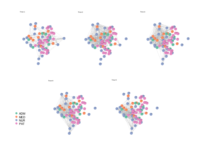
Figure 1: The RFID sensors data: the 5 networks obtained by combining together the information within each of the five 24-hour periods. The four different identities of the individuals are marked in four different colours.

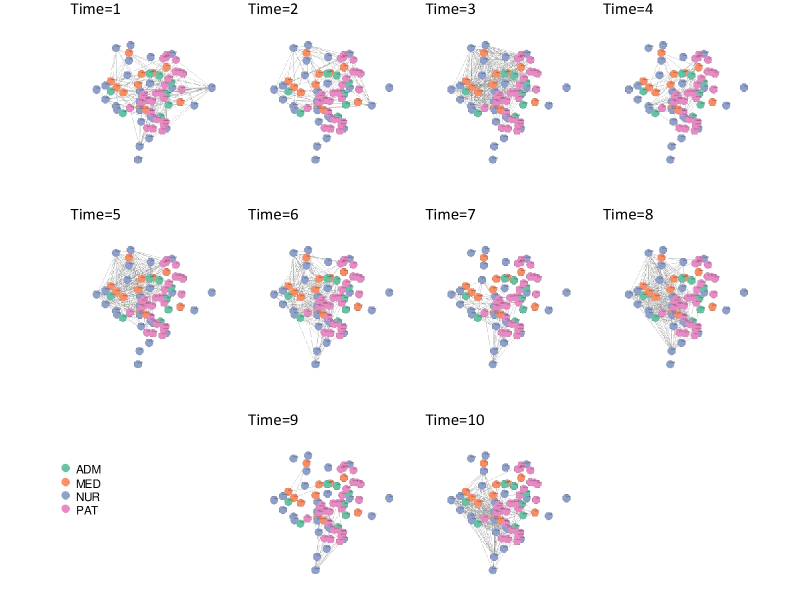
Figure 2: The RFID sensors data: the 10 networks obtained by combining together the information within each of the ten 12-hour periods. The four different identities of the individuals are marked in four different colours.

5.2 French high school contact data

Now we consider a contact network data collected in a high school in Marseilles, France (Mastrandrea et al.,, 2015). The data are the recorded face-to-face contacts among the students from 9 classes during $n=5$ days in December 2013, measured by the SocioPatterns infrastructure. Those are students in the so-called classes preparatoires – a part of the French post-secondary education system. We label the 3 classes majored in mathematics and physics as MP1, MP2 and MP3, the 3 classes majored in biology as BIO1, BIO2 and BIO3, the 2 classes majored in physics and chemistry as PC1 and PC2, and the class majored in engineering as EGI. The data are available at www.sociopatterns.org/datasets/high-school-contact-and-friendship-networks/. We have removed the individuals with missing values, and include the remaining $p=327$ students in our clustering analysis based on the AR(1) stochastic block network model (see Definition 3.1).

We start the analysis with $q=2$. The detected 2 clusters by the spectral clustering algorithm (SCA) based on either $\widehat{\mathbf{L}}$ in (3.6) or $\bar{\mathbf{X}}$ are reported in Table 5. The two methods lead to almost identical results: 3 classes majored in biology are in one cluster and the other 6 classes are in the other cluster. The number of ‘misplaced’ students is 2 and 1, respectively, by the SCA based on $\widehat{\mathbf{L}}$ and $\bar{\mathbf{X}}$. Figure 3 shows that the identified two clusters are clearly separated from each other across all the 5 days. The permutation test (2.13) on the residuals indicates that the stationary AR(1) stochastic block network model seems to be appropriate for this data set, as the $P$-value is 0.676. We repeat the analysis for $q=3$, leading to equally plausible results: 3 biology classes are in one cluster, 3 mathematics and physics classes are in another cluster, and the 3 remaining classes form the 3rd cluster. See also Figure 4 for the graphical illustration with the 3 clusters.

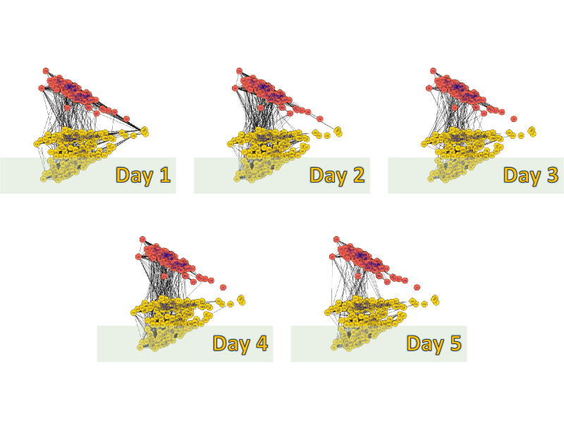
Figure 3: French high school contact networks over 5 days: the nodes marked in two colours represent the $q=2$ clusters determined by SCA based on $\widehat{\mathbf{L}}$ in (3.4).

Table 5: French high school contact network data: the detected clusters by spectral clustering algorithm (SCA) based on either $\widehat{\mathbf{L}}$ in (3.4) or $\bar{\mathbf{X}}$. The number of clusters is set at $q=2$.

	SCA based on $\widehat{\mathbf{L}}$		SCA based on $\bar{X}$
Class	Cluster 1	Cluster 2	Cluster 1	Cluster 2
BIO1	0	37	1	36
BIO2	1	32	0	33
BIO3	1	39	0	40
MP1	33	0	33	0
MP2	29	0	29	0
MP3	38	0	38	0
PC1	44	0	44	0
PC2	39	0	39	0
EGI	34	0	34	0

To choose the number of clusters $q$ objectively, we define the Bayesian information criteria (BIC) as follows:

$${\rm BIC}(q)=-2\max\,\log({\rm likelihood})+\log\{n(p/q)^{2}\}q(q+1).$$

For each fixed $q$, we effectively build $q(q+1)/2$ models independently and each model has 2 parameters $\theta_{k,\ell}$ and $\eta_{k,\ell}$, $1\leq k\leq\ell\leq q$. The number of the available observations for each model is approximately $n(p/q)^{2}$, assuming that the numbers of nodes in all the $q$ clusters are about the same, which is then $p/q$. Thus the penalty term in the BIC above is $\sum_{1\leq k\leq\ell\leq q}2\log\{n(p/q)^{2}\}=\log\{n(p/q)^{2}\}q(q+1)$.

Table 6 lists the values of BIC($q$) for different $q$. The minimum is obtained at $q=9$, exactly the number of original classes in the school. Performing the SCA based on $\widehat{\mathbf{L}}$ with $q=9$, we obtain almost perfect classification: all the 9 original classes are identified as the 9 clusters with only in total 4 students being placed outside their own classes. Figure 5 plots the networks with the identified 9 clusters in 9 different colours. The estimated $\theta_{i,j}$ and $\eta_{i,j}$, together with their standard errors calculated based on the asymptotic normality presented in Theorem 4, are reported in Table 7. As $\widehat{\theta}_{i,j}$ for $i\neq j$ are very small (i.e. $\leq 0.027$), the students from different classes who have not contacted with each other are unlikely to contact next day. See (3.1) and (2.3). On the other hand, as $\widehat{\eta}_{i,j}$ for $i\neq j$ are large (i.e. $\geq 0.761$), the students from different classes who have contacted with each other are likely to lose the contacts next day. Note that $\widehat{\theta}_{i,i}$ are greater than $\widehat{\theta}_{i,j}$ for $i\neq j$ substantially, and $\widehat{\eta}_{i,i}$ are smaller than $\widehat{\eta}_{i,j}$ for $i\neq j$ substantially. This implies that the students in the same class are more likely to contact with each other than those across the different classes.

Table 6: Fitting AR(1) stochastic block models to the French high school data: BIC values for different cluster numbers $q$.

$q$	2	3	5	7	8	9	10	11
BIC($q$)	43624	40586	37726	36112	35224	34943	35002	35120

To apply the variational EM algorithm of Matias and Miele, (2017) to analyze this data set, we use the R package dynsbm. The algorithm is designed to identify time-varying dynamic stochastic block structure in the sense that both the membership of nodes and the transition probabilities may vary with time. Furthermore it also identifies the nodes not belonging to any clusters. The number of the clusters selected by the so-called integrated classification likelihood criterion is also 9. The identified 9 clusters are always dominated by the 9 original classes in the school, though they vary from day to day. The number of the identified students not belonging to any of the 9 clusters was 15, 17, 24, 32 and 28, respectively, in those 5 days. Furthermore the number of the students who were not put in their own classes was 14, 9, 12, 10 and 12, respectively. The more detailed results are reported in Appendix B. Those findings are less clear-cut than those obtained from our method above. This is hardly surprising as Matias and Miele, (2017) adopts a general setting without imposing stationarity.

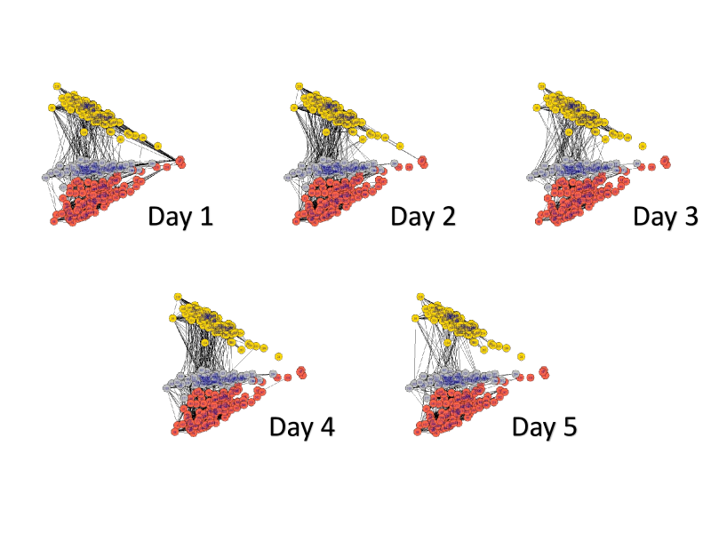
Figure 4: French high school contact networks over 5 days: the nodes marked in three colours represent the $q=3$ clusters determined by SCA based on $\widehat{\mathbf{L}}$ in (3.4).

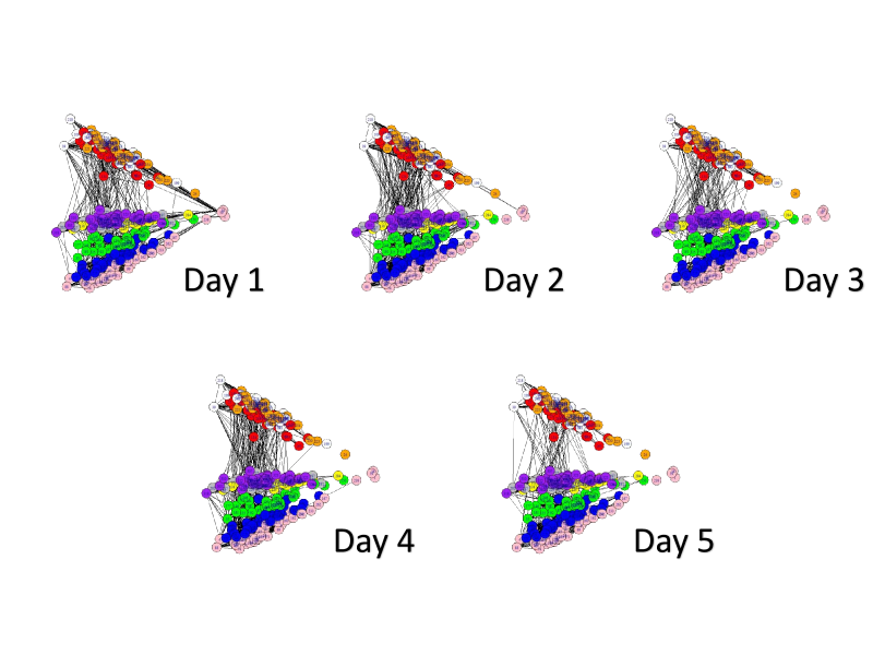
Figure 5: French high school contact networks over 5 days: the nodes marked in seven colours represent the $q=9$ clusters determined by SCA based on $\widehat{\mathbf{L}}$ in (3.4).

Table 7: Fitting AR(1) stochastic block models with $q=9$ clusters to the French high school data: the estimation parameters and their standard errors (in parentheses).

	Cluster	1	2	3	4	5	6	7	8	9
	1	.246	.001	.004	.006	.001	.009	.003	.024	.003
		(.008)	(.001)	(.001)	(.001)	(.001)	(.001)	(.001)	(.002)	(.001)
	2		.136	.024	.0018	.001	.007	.001	.001	.027
			(.009)	(.002)	(.001)	(.001)	(.001)	(.000)	(.001)	(.002)
	3			.252	.001	.002	.007	.001	.001	.022
				(.011)	(.001)	(.001)	(.001)	(.001)	(.001)	(.002)
	4				.234	.020	.001	.024	.002	.001
					(.010)	(.002)	(.001)	(.002)	(.001)	(.001)
$\widehat{\theta}_{i,j}$	5					.196	.001	.020	.002	.004
						(.008)	(.001)	(.002)	(.000)	(.001)
	6						.181	.001	.010	.007
							(.008)	(.001)	(.001)	(.001)
	7							.252	.003	.006
								(.009)	(.001)	(.001)
	8								.202	.001
									(.006)	(.001)
	9									.219
										(.008)
	1	.563	.999	.959	.976	.999	.867	.870	.792	.909
		(.015)	(.001)	(.036)	(.098)	(.001)	(.054)	(.001)	(.000)	(.051)
	2		.472	.761	.888	.999	.866	.999	.999	.866
			(.024)	(.036)	(.097)	(.001)	(.054)	(.001)	(.000)	(.026)
	3			.453	.999	.928	.864	.999	.999	.772
				(.016)	(.000)	(.066)	(.048)	(.000)	(.000)	(.031)
	4				.509	.868	.999	.784	.956	.999
					(.017)	(.028)	(.000)	(.029)	(.041)	(.000)
$\widehat{\eta}_{i,j}$	5					.544	.999	.929	.842	.935
						(.017)	(.001)	(.021)	(.078)	(.041)
	6						.589	.999	.793	.923
							(.019)	(.001)	(.040)	(.036)
	7							.480	.999	.814
								(.014)	(.000)	(.051)
	8								.504	.999
									(.127)	(.000)
	9									.471
										(.014)

5.3 Global trade data

Our last example concerns the annual international trades among $p=197$ countries between 1950 and 2014 (i.e. $n=65$). We define an edge between two countries to be 1 as long as there exist trades between the two countries in that year (regardless the direction), and 0 otherwise. We take this simplistic approach to illustrate our AR(1) stochastic block model with a change point. The data used are a subset of the openly available trade data for 205 countries in 1870 – 2014 (Barbieri et al.,, 2009; Barbieri and Keshk,, 2016). We leave out several countries, e.g. Russia and Yugoslavia, which did not exist for the whole period concerned.

Setting $q=2$, we fit the data with an AR(1) stochastic block model with two clusters. The $P$-value of the permutation test for the residuals resulted from the fitted model is 0, indicating overwhelmingly that the stationarity does not hold for the whole period. Applying the maximum likelihood estimator (3.15), the estimated change point is at year 1991. Before this change point, the identified Cluster I contains 26 countries, including the most developed industrial countries such as USA, Canada, UK and most European countries. Cluster II contains 171 countries, including all African and Latin American countries, and most Asian countries. After 1991, 41 countries switched from Cluster II to Cluster I, including Argentina, Brazil, Bulgaria, China, Chile, Columbia, Costa Rica, Cyprus, Hungary, Israel, Japan, New Zealand, Poland, Saudi Arabia, Singapore, South Korea, Taiwan, and United Arab Emirates. There was no single switch from Cluster I to II. Note that 1990 may be viewed as the beginning of the globalization. With the collapse of the Soviet Union in 1989, the fall of Berlin Wall and the end of the Cold War in 1991, the world became more interconnected. The communist bloc countries in East Europe, which had been isolated from the capitalist West, began to integrate into the global market economy. Trade and investment increased, while barriers to migration and to cultural exchange were lowered.

Figure 6 presents the average adjacency matrix of the 197 countries before and after the change point, where the cold blue color indicates small value and the warm red color indicates large value. Before 1991, there are only 26 countries in Cluster 1. The intensive red in the small lower left corner indicates the intensive trades among those 26 countries. After 1991, the densely connected lower left corner is enlarged as now there are 67 countries in Cluster 1. Note some members of Cluster 2 also trade with the members of Cluster 1, though not all intensively.

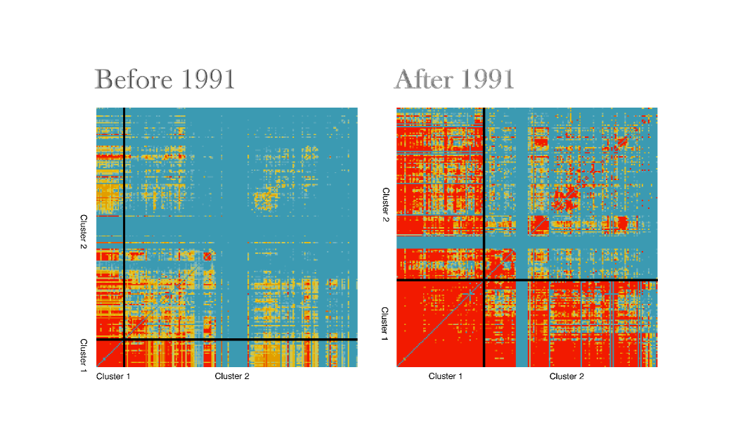
Figure 6: Average adjacency matrix for the trades among the 197 countries before and after 1991. The values from 0 to 1 are colour-coded from blue, light blue, light red to red.

The estimated parameters for the fitted AR(1) stochastic block model with $q=2$ clusters are reported in Table 8. Since estimated values for $\widehat{\theta}_{1,2},\widehat{\eta}_{1,2}$ before and after the change point are always small, the trading status between the countries across the two clusters are unlikely to change. Nevertheless $\widehat{\theta}_{1,2}$ is 0.154 after 1991, and 0.053 before 1991; indicating greater possibility for new trades to happen after 1991.

Table 8: Fitting AR(1) stochastic block model with a change point and $q=2$ to the Global trade data: the estimated AR coefficients before and after 1991.

	$t\leq 1991$		$t>1991$
Coefficients	Estimates	SE	Estimates	SE
$\theta_{1,1}$	.062	.0092	.046	.0005
$\theta_{1,2}$	.053	.0008	.154	.0013
$\theta_{2,2}$	.023	.0002	.230	.0109
$\eta_{1,1}$	.003	.0005	.144	.0016
$\eta_{1,2}$	.037	.0008	.047	.0007
$\eta_{2,2}$	.148	.0012	.006	.0003

A final remark. We proposed in this paper a simple AR(1) setting to represent the dynamic dependence in network data explicitly. It also facilitates easy inference such as the maximum likelihood estimation and model diagnostic checking. A new class of dynamic stochastic block models illustrates the usefulness of the setting in handling more complex underlying structures including structure breaks due to change points.

It is conceivable to construct AR($p$) or even ARMA network models following the similar lines. However a more fertile exploration is perhaps to extend the setting for the networks with dependent edges, incorporating in the model some stylized features of network data such as transitivity, homophily. The development in this direction will be reported in a follow-up paper. On the other hand, dynamic networks with weighted edges may be treated as matrix time series for which effective modelling procedures have been developed based on various tensor decompositions (Wang et al.,, 2019; Chang et al., 2020a, ).

“Autoregressive Networks” by B. Jiang, J. Li and Q. Yao

Appendix: Technical proofs and further real data analysis

A.1 Proof of Proposition 1

Note all $X_{i,j}^{t}$ take binary values 0 or 1. Hence

$$P(X_{i,j}^{1}=1)=P(X_{i,j}^{0}=1)P(X_{i,j}^{1}=1|X_{i,j}^{0}=1)+P(X_{i,j}^{0}=0)P(X_{i,j}^{1}=1|X_{i,j}^{0}=0)$$

$$= \pi_{i,j}(1-\beta_{i,j})+(1-\pi_{i,j})\alpha_{i,j}={\alpha_{i,j}\over\alpha_{i,j}+\beta_{i,j}}(1-\beta_{i,j})+{\beta_{i,j}\over\alpha_{i,j}+\beta_{i,j}}\alpha_{i,j}={\alpha_{i,j}\over\alpha_{i,j}+\beta_{i,j}}=\pi_{i,j}.$$

Thus ${\mathcal{L}}(X_{i,j}^{1})={\mathcal{L}}(X_{i,j}^{0})$. Since all ${\mathbf{X}}^{t}$ are Erdós-Renyi, ${\mathcal{L}}({\mathbf{X}}^{1})={\mathcal{L}}({\mathbf{X}}^{0})$. Condition (2.5) ensures that $\{{\mathbf{X}}_{t}\}$ is a homogeneous Markov chain. Hence ${\mathcal{L}}({\mathbf{X}}^{t})={\mathcal{L}}({\mathbf{X}}^{0})$ for any $t\geq 1$. This implies the required stationarity.

As $E(X_{i,j}^{t})=P(X_{i,j}^{t}=1)$, and ${\rm Var}(X_{i,j}^{t})=E(X_{i,j}^{t})-\{E(X_{i,j}^{t})\}^{2}$, (2.8) follows from the stationarity, (2.6) and (2.7).

Note that (2.1) implies a Yule-Walker equation

$$\gamma_{i,j}(k)=(1-\alpha_{i,j}-\beta_{i,j})\gamma_{i,j}(k-1),\quad k=1,2,\cdots,$$ (A.1)

where $\gamma_{i,j}(k)={\rm Cov}(X_{i,j}^{t+k},X_{i,j}^{t})$.

Since the networks are all Erdös-Renyi, (2.9) follows from the Yule-Walker equation (A.1) immediately, noting $\rho_{i,j}(k)=\gamma_{i,j}(k)/\gamma_{i,j}(0)$ and $\rho_{i,j}(0)=1$. To prove (A.1), it follows from (2.1) that for any $k\geq 1$,

$$E(X_{i,j}^{t+k}X_{i,j}^{t}) =E(X_{i,j}^{t+k-1}X_{i,j}^{t})P({\varepsilon}_{i,j}^{t+k}=0)+P({\varepsilon}_{i,j}^{t+k}=1)EX_{i,j}^{t}$$

$$=(1-\alpha_{i,j}-\beta_{i,j})E(X_{i,j}^{t+k-1}X_{i,j}^{t})+\alpha_{i,j}^{2}/(\alpha_{i,j}+\beta_{i,j}).$$

Thus

$$\gamma_{i,j}(k) =E(X_{i,j}^{t+k}X_{i,j}^{t})-(EX_{i,j}^{t})^{2}=E(X_{i,j}^{t+k}X_{i,j}^{t})-{\alpha_{i,j}^{2}\over(\alpha_{i,j}+\beta_{i,j})^{2}}$$

$$=(1-\alpha_{i,j}-\beta_{i,j})E(X_{i,j}^{t+k-1}X_{i,j}^{t})+{\alpha_{i,j}^{2}\over\alpha_{i,j}+\beta_{i,j}}(1-{1\over\alpha_{i,j}+\beta_{i,j}})$$

$$=(1-\alpha_{i,j}-\beta_{i,j})\{E(X_{i,j}^{t+k-1}X_{i,j}^{t})-{\alpha_{i,j}^{2}\over(\alpha_{i,j}+\beta_{i,j})^{2}}\}=(1-\alpha_{i,j}-\beta_{i,j})\gamma_{i,j}(k-1).$$

This completes the proof.

A.2 Proof of Proposition 2

We only prove (2.11), as (2.10) follows from (2.11) immediately. To prove (2.11), we only need to show

$$d_{i,j}(k)\equiv P(X_{i,j}^{t}\neq X_{i,j}^{t+k})={2\alpha_{i,j}\beta_{i,j}\over(\alpha_{i,j}+\beta_{i,j})^{2}}\{1-(1-\alpha_{i,j}-\beta_{i,j})^{k}\},\quad k=1,2,\cdots.$$ (A.2)

We Proceed by induction. It is easy to check that (A.2) holds for $k=1$. Assuming it also holds for $k\geq 1$, then

$$d_{i,j}(k+1)=P(X_{i,j}^{t}=0,X_{i,j}^{t+k+1}=1)+P(X_{i,j}^{t}=1,X_{i,j}^{t+k+1}=0)$$

$$= \,P(X_{i,j}^{t}=0,X_{i,j}^{t+k}=1,X_{i,j}^{t+k+1}=1)+P(X_{i,j}^{t}=0,X_{i,j}^{t+k}=0,X_{i,j}^{t+k+1}=1)$$

$$+P(X_{i,j}^{t}=1,X_{i,j}^{t+k}=0,X_{i,j}^{t+k+1}=0)+P(X_{i,j}^{t}=1,X_{i,j}^{t+k}=1,X_{i,j}^{t+k+1}=0)$$

$$= \,P(X_{i,j}^{t}=0,X_{i,j}^{t+k}=1)(1-\beta_{i,j})+\{P(X_{i,j}^{t}=0)-P(X_{i,j}^{t}=0,X_{i,j}^{t+k}=1)\}\alpha_{i,j}$$

$$+P(X_{i,j}^{t}=1,X_{i,j}^{t+k}=0)(1-\alpha_{i,j})+\{P(X_{i,j}^{t}=1)-P(X_{i,j}^{t}=1,X_{i,j}^{t+k}=0)\}\beta_{i,j}$$

$$= \,\{P(X_{i,j}^{t}=0,X_{i,j}^{t+k}=1)+P(X_{i,j}^{t}=1,X_{i,j}^{t+k}=0)\}(1-\alpha_{i,j}-\beta_{i,j})+{2\alpha_{i,j}\beta_{i,j}\over\alpha_{i,j}+\beta_{i,j}}$$

$$= \,d_{i,j}(k)(1-\alpha_{i,j}-\beta_{i,j})+{2\alpha_{i,j}\beta_{i,j}\over\alpha_{i,j}+\beta_{i,j}}\,=\,{2\alpha_{i,j}\beta_{i,j}\over(\alpha_{i,j}+\beta_{i,j})^{2}}\{1-(1-\alpha_{i,j}-\beta_{i,j})^{k+1}\}.$$

Hence (A.2) also holds for $k+1$. This completes the proof.

A.3 Proof of Proposition 3

Proof.

Note that for any nonempty elements $A\in{\mathcal{F}}_{0}^{k},B\in{\mathcal{F}}_{k+\tau}^{\infty}$, there exist $A_{0}\in{\mathcal{F}}_{0}^{k-1}$ and $B_{0}\in{\mathcal{F}}_{k+\tau+1}^{\infty}$ such that $A=A_{0}\times\{0\},A_{0}\times\{1\},$ or $A_{0}\times\{0,1\}$, and $B=B_{0}\times\{0\},B_{0}\times\{1\},$ or $B_{0}\times\{0,1\}$. We first consider the case where $B=B_{0}\times\{x_{k}\}$ and $A=A_{0}\times\{x_{k+\tau}\}$ where $x_{k},x_{k+\tau}=0$ or $1$. Note that

$$P(A_{0},X^{k}_{i,j}=x_{k},B_{0},X_{i,j}^{k+\tau}=x_{k+\tau})$$

$$= P(B_{0}|X_{i,j}^{k+\tau}=x_{k+\tau})P(X_{i,j}^{k+\tau}=x_{k+\tau},A_{0},X_{i,j}^{k}=x_{k})$$

$$= P(B_{0},X_{i,j}^{k+\tau}=x_{k+\tau})P(A_{0},X^{k}_{i,j}=x_{k})\cdot\frac{P(X_{i,j}^{k+\tau}=x_{k+\tau}|X_{i,j}^{k}=x_{k})}{P(X_{i,j}^{k+\tau}=x_{k+\tau})}$$

$$= P(B_{0},X_{i,j}^{k+\tau}=x_{k+\tau})P(A_{0},X^{k}_{i,j}=x_{k})\cdot\frac{P(X_{i,j}^{k+\tau}=x_{k+\tau},X_{i,j}^{k}=x_{k})}{P(X_{i,j}^{k+\tau}=x_{k+\tau})P(X_{i,j}^{k}=x_{k})}$$

On the other hand, note that

$$P(X_{i,j}^{k+\tau}=1,X_{i,j}^{k}=1)-P(X_{i,j}^{k+\tau}=1)P(X_{i,j}^{k}=1)=\rho_{i,j}(\tau);$$

$$P(X_{i,j}^{k+\tau}=1,X_{i,j}^{k}=0)-P(X_{i,j}^{k+\tau}=1)P(X_{i,j}^{k}=0)$$

$$= P(X_{i,j}^{k+\tau}=1)-P(X_{i,j}^{k+\tau}=1,X_{i,j}^{k}=1)-P(X_{i,j}^{k+\tau}=1)[1-P(X_{i,j}^{k}=1)]$$

$$= -\rho_{i,j}(\tau);$$

$$P(X_{i,j}^{k+\tau}=0,X_{i,j}^{k}=1)-P(X_{i,j}^{k+\tau}=0)P(X_{i,j}^{k}=1)$$

$$= P(X_{i,j}^{k}=1)-P(X_{i,j}^{k+\tau}=1,X_{i,j}^{k}=1)-[1-P(X_{i,j}^{k+\tau}=1)]P(X_{i,j}^{k}=1)$$

$$= -\rho_{i,j}(\tau);$$

$$P(X_{i,j}^{k+\tau}=0,X_{i,j}^{k}=0)-P(X_{i,j}^{k+\tau}=0)P(X_{i,j}^{k}=0)$$

$$= P(X_{i,j}^{k+\tau}=0)-P(X_{i,j}^{k+\tau}=0,X_{i,j}^{k}=1)-P(X_{i,j}^{k+\tau}=0)[1-P(X_{i,j}^{k}=1)]$$

$$= \rho_{i,j}(\tau).$$

Consequently, we have

$$|P(A_{0},X^{k}_{i,j}=x_{k},B_{0},X_{i,j}^{k+\tau}=x_{k+\tau})-P(A_{0},X^{k}_{i,j}=x_{k})P(B_{0},X_{i,j}^{k+\tau}=x_{k+\tau})|$$

$$= \left|P(A_{0},X^{k}_{i,j}=x_{k})P(B_{0},X_{i,j}^{k+\tau}=x_{k+\tau})\left[\frac{P(X_{i,j}^{k+\tau}=x_{k+\tau},X_{i,j}^{k}=x_{k})}{P(X_{i,j}^{k+\tau}=x_{k+\tau})P(X_{i,j}^{k}=x_{k})}-1\right]\right|$$

$$\leq \rho_{i,j}(\tau).$$

In the case where $A=A_{0}\times\{0,1\}$ and/or $B=B_{0}\times\{0,1\}$, since $A$ and $B$ are nonempty, there exist integers $0<k_{1}<k$ and/or $k_{2}>k+1$, and correspondingly $A_{1}\in{\mathcal{F}}_{0}^{k_{1}-1}\times\{x_{k_{1}}\}$ and/or $B\in{\mathcal{F}}_{k_{2}+\tau+1}^{\infty}\times\{x_{k_{2}+\tau}\}$ with $x_{k_{1}},x_{k_{2}+\tau}=0~{}{\rm or}~{}1$, such that $P(A\cap B)-P(A)P(B)=P(A_{1}\cap B_{1})-P(A_{1})P(B_{1})$. Following similar arguments above we have $P(A\cap B)-P(A)P(B)\leq\rho_{i,j}(\tau+k_{2}-k_{1})<\rho_{ij}(\tau)$. We thus proved that $\alpha^{i,j}(\tau)\leq\rho_{i,j}(\tau)$. The conclusion of Proposition 3 follows from Proposition 1. ∎

A.4 Proof of Proposition 4

We introduce some technical lemmas first.

Lemma 1.

For any $(i,j)\in{\mathcal{J}}$, denote $Y_{i,j}^{t}:=X_{i,j}^{t}(1-X_{i,j}^{t-1})$, and let ${\bf Y}_{t}=(Y_{i,j}^{t})_{1\leq i,j\leq p}$ be the $p\times p$ matrix at time t. Under the assumptions of Proposition 1, we have $\{{\bf Y}_{t},t=1,2\ldots\}$ is stationary such that for any $(i,j),(l,m)\in{\mathcal{J}}$, and $t,s\geq 1$, $t\neq s$,

$$EY_{i,j}^{t}=\frac{\alpha_{i,j}\beta_{i,j}}{\alpha_{i,j}+\beta_{i,j}},~{}~{}~{}{\rm Var}(Y_{i,j}^{t})=\frac{\alpha_{i,j}\beta_{i,j}(\alpha_{i,j}+\beta_{i,j}-\alpha_{i,j}\beta_{i,j})}{(\alpha_{i,j}+\beta_{i,j})^{2}},$$

$$\rho_{Y_{i,j}}(|t-s|)\equiv{\rm Corr}(Y_{i,j}^{t},Y_{lm}^{s})=\begin{cases}-\frac{\alpha_{i,j}\beta_{i,j}(1-\alpha_{i,j}-\beta_{i,j})^{|t-s|-1}}{\alpha_{i,j}+\beta_{i,j}-\alpha_{i,j}\beta_{i,j}}&{\rm if}~{}~{}(i,j)=(l,m),\\ 0&{\rm otherwise}.\end{cases}$$

Proof.

Note that $Y_{i,j}^{t}=X_{i,j}^{t}(1-X_{i,j}^{t-1})=(1-X_{i,j}^{t-1})I({\varepsilon}_{i,j}^{t}=1)$. We thus have:

$E(Y_{i,j}^{t})=P(X_{i,j}^{t-1}=0)\alpha_{i,j}=(1-EX_{i,j}^{t-1})\alpha_{i,j}=\frac{\alpha_{i,j}\beta_{i,j}}{\alpha_{i,j}+\beta_{i,j}}$.

${\rm Var}(Y_{i,j}^{t})=E(Y_{i,j}^{t})[1-E(Y_{i,j}^{t})]=\frac{\alpha_{i,j}\beta_{i,j}}{\alpha_{i,j}+\beta_{i,j}}\left(1-\frac{\alpha_{i,j}\beta_{i,j}}{\alpha_{i,j}+\beta_{i,j}}\right)=\frac{\alpha_{i,j}\beta_{i,j}(\alpha_{i,j}+\beta_{i,j}-\alpha_{i,j}\beta_{i,j})}{(\alpha_{i,j}+\beta_{i,j})^{2}}$.

For $k=1$ we have $E(Y_{i,j}^{t}Y_{i,j}^{t+1})=E[(1-X_{i,j}^{t-1})X_{i,j}^{t}(1-X_{i,j}^{t})X_{i,j}^{t+1}]=0$. For any $k\geq 2$, using the fact that $E(X_{ij}^{t}X_{ij}^{t+k})={\alpha_{ij}\over(\alpha_{ij}+\beta_{ij})^{2}}\{\beta_{ij}(1-\alpha_{ij}-\beta_{ij})^{k}+\alpha_{ij}\}$, we have

$$E(Y_{i,j}^{t}Y_{i,j}^{t+k}) = E[X_{i,j}^{t}(1-X_{i,j}^{t-1})(1-X_{i,j}^{t+k-1})I({\varepsilon}_{i,j}^{t+k}=1)]$$

$$= \alpha_{i,j}E[X_{i,j}^{t}(1-X_{i,j}^{t-1})(1-X_{i,j}^{t+k-1})]$$

$$= \alpha_{i,j}P(X_{i,j}^{t+k-1}=0|X_{i,j}^{t}=1)P(X_{i,j}^{t}=1|X_{i,j}^{t-1}=0)P(X_{i,j}^{t-1}=0)$$

$$= \frac{\alpha_{i,j}^{2}\beta_{i,j}}{\alpha_{i,j}+\beta_{i,j}}[1-P(X_{i,j}^{t+k-1}=1|X_{i,j}^{t}=1)]$$

$$= \frac{\alpha_{i,j}^{2}\beta_{i,j}}{\alpha_{i,j}+\beta_{i,j}}\left[1-\frac{E(X_{i,j}^{t+k-1}X_{i,j}^{t})}{EX_{i,j}^{t}}\right]$$

$$= \frac{\alpha_{i,j}^{2}\beta_{i,j}}{\alpha_{i,j}+\beta_{i,j}}\left[1-\frac{\beta_{i,j}(1-\alpha_{i,j}-\beta_{i,j})^{k-1}+\alpha_{i,j}}{\alpha_{i,j}+\beta_{i,j}}\right]$$

$$= \frac{\alpha_{i,j}^{2}\beta_{i,j}^{2}[1-(1-\alpha_{i,j}-\beta_{i,j})^{k-1}]}{(\alpha_{i,j}+\beta_{i,j})^{2}}.$$

Therefore we have for any $k\geq 1$,

$${\rm Cov}(Y_{i,j}^{t},Y_{i,j}^{t+k}) = E(Y_{i,j}^{t}Y_{i,j}^{t+k})-EY_{i,j}^{t}EY_{i,j}^{t+k}$$

$$= \frac{\alpha_{i,j}^{2}\beta_{i,j}^{2}[1-(1-\alpha_{i,j}-\beta_{i,j})^{k-1}]}{(\alpha_{i,j}+\beta_{i,j})^{2}}-\frac{\alpha_{i,j}^{2}\beta_{i,j}^{2}}{(\alpha_{i,j}+\beta_{i,j})^{2}}$$

$$= -\frac{\alpha_{i,j}^{2}\beta_{i,j}^{2}(1-\alpha_{i,j}-\beta_{i,j})^{k-1}}{(\alpha_{i,j}+\beta_{i,j})^{2}}.$$

Consequently, for any $|t-s|=1,2,\ldots$, the ACF of the process $\{Y_{i,j}^{t},t=1,2\ldots\}$ is given as:

$$\rho_{Y_{i,j}}(|t-s|) = -\frac{\alpha_{i,j}^{2}\beta_{i,j}^{2}(1-\alpha_{i,j}-\beta_{i,j})^{|t-s|-1}}{(\alpha_{i,j}+\beta_{i,j})^{2}}\cdot\frac{(\alpha_{i,j}+\beta_{i,j})^{2}}{\alpha_{i,j}\beta_{i,j}(\alpha_{i,j}+\beta_{i,j}-\alpha_{i,j}\beta_{i,j})}$$

$$= -\frac{\alpha_{i,j}\beta_{i,j}(1-\alpha_{i,j}-\beta_{i,j})^{|t-s|-1}}{\alpha_{i,j}+\beta_{i,j}-\alpha_{i,j}\beta_{i,j}}.$$

∎

Since the mixing property is hereditary, $Y_{i,j}^{t}$ is also $\alpha$-mixing. From Proposition 3 and Theorem 1 of Merlevède et al., (2009), we obtain the following concentration inequalities:

Lemma 2.

Let conditions (2.5) and C1 hold. There exist positive constants $C_{1}$ and $C_{2}$ such that for all $n\geq 4$ and ${\varepsilon}<\frac{1}{(\log n)(\log\log n)}$,

$$P\left(\left|n^{-1}\sum_{t=1}^{n}X_{i,j}^{t}-EX_{i,j}^{t}\right|>{\varepsilon}\right)\leq\exp\{-C_{1}n{\varepsilon}^{2}\},$$

$$P\left(\left|n^{-1}\sum_{t=1}^{n}Y_{i,j}^{t}-EY_{i,j}^{t}\right|>{\varepsilon}\right)\leq\exp\{-C_{2}n{\varepsilon}^{2}\}.$$

Now we are ready to prove Proposition 4.

Proof of Proposition 4:

Let ${\varepsilon}=C\sqrt{\frac{\log p}{n}}$ with $C^{2}C_{1}>2$ and $C^{2}C_{2}>2$. Note that under condition (C2) we have ${\varepsilon}=o\big{(}\frac{1}{(\log n)(\log\log n)}\big{)}$. Consequently by Lemma 2, Proposition 1 and Lemma 1, we have

$$P\left(\left|n^{-1}\sum_{t=1}^{n}X_{i,j}^{t}-\frac{\alpha_{i,j}}{\alpha_{i,j}+\beta_{i,j}}\right|>C\sqrt{\frac{\log p}{n}}\right)\leq\exp\{-C^{2}C_{1}\log p\},$$

$$P\left(\left|n^{-1}\sum_{t=1}^{n}Y_{i,j}^{t}-\frac{\alpha_{i,j}\beta_{i,j}}{\alpha_{i,j}+\beta_{i,j}}\right|>C\sqrt{\frac{\log p}{n}}\right)\leq\exp\{-C^{2}C_{2}\log p\}.$$

Consequently, with probability greater than $1-\exp\{-C^{2}C_{1}\log p\}-\exp\{-C^{2}C_{2}\log p\}$,

$$\frac{\frac{\alpha_{i,j}\beta_{i,j}}{\alpha_{i,j}+\beta_{i,j}}-C\sqrt{\frac{\log p}{n}}}{\frac{\beta_{i,j}}{\alpha_{i,j}+\beta_{i,j}}+\frac{1}{n}+C\sqrt{\frac{\log p}{n}}}\leq\widehat{\alpha}_{i,j}\leq\frac{\frac{\alpha_{i,j}\beta_{i,j}}{\alpha_{i,j}+\beta_{i,j}}+C\sqrt{\frac{\log p}{n}}}{\frac{\beta_{i,j}}{\alpha_{i,j}+\beta_{i,j}}-\frac{1}{n}-C\sqrt{\frac{\log p}{n}}}.$$

Note that when $n$ and $\frac{n}{\log p}$ are large enough such that, $\frac{1}{n}\leq C\sqrt{\frac{\log p}{n}}\leq l/4$, we have

$$\alpha_{i,j}-\frac{\frac{\alpha_{i,j}\beta_{i,j}}{\alpha_{i,j}+\beta_{i,j}}-C\sqrt{\frac{\log p}{n}}}{\frac{\beta_{i,j}}{\alpha_{i,j}+\beta_{i,j}}+\frac{1}{n}+C\sqrt{\frac{\log p}{n}}}\leq\frac{2C\alpha_{i,j}\sqrt{\frac{\log p}{n}}+C\sqrt{\frac{\log p}{n}}}{\frac{\beta_{i,j}}{\alpha_{i,j}+\beta_{i,j}}}\leq 3l^{-1}C\sqrt{\frac{\log p}{n}},$$

and

$$\frac{\frac{\alpha_{i,j}\beta_{i,j}}{\alpha_{i,j}+\beta_{i,j}}+C\sqrt{\frac{\log p}{n}}}{\frac{\beta_{i,j}}{\alpha_{i,j}+\beta_{i,j}}-\frac{1}{n}-C\sqrt{\frac{\log p}{n}}}-\alpha_{i,j}\leq\frac{2C\alpha_{i,j}\sqrt{\frac{\log p}{n}}+C\sqrt{\frac{\log p}{n}}}{\frac{\beta_{i,j}}{\alpha_{i,j}+\beta_{i,j}}-\frac{l}{2}}\leq 6l^{-1}C\sqrt{\frac{\log p}{n}},$$

Therefore we conclude that when when $n$ and $\frac{n}{\log p}$ are large enough,

$$P\left(|\widehat{\alpha}_{i,j}-\alpha_{i,j}|\geq 6l^{-1}C\sqrt{\frac{\log p}{n}}\right)\leq\exp\{-C^{2}C_{1}\log p\}+\exp\{-C^{2}C_{2}\log p\}.$$ (A.3)

As a result, we have

$$P\left(\max_{(i,j)\in{\mathcal{J}}}|\widehat{\alpha}_{i,j}-\alpha_{i,j}|<6l^{-1}C\sqrt{\frac{\log p}{n}}\right)\geq 1-p^{2}\exp\{-C^{2}C_{1}\log p\}-p^{2}\exp\{-C^{2}C_{2}\log p\}\rightarrow 1.$$

Consequently we have $\max_{(i,j)\in{\mathcal{J}}}|\widehat{\alpha}_{i,j}-\alpha_{i,j}|=O_{p}\left(\sqrt{\frac{\log p}{n}}\right)$. Convergence of $\widehat{\beta}_{i,j}$ can be proved similarly.

A.5 Proof of Proposition 5

Note that the log-likelihood function for $(\alpha_{i,j},\beta_{i,j})$ is:

$$l(\alpha_{i,j},\beta_{i,j}) =\log(\alpha_{i,j})\sum_{t=1}^{n}X_{i,j}^{t}(1-X_{i,j}^{t-1})+\log(1-\alpha_{i,j})\sum_{t=1}^{n}(1-X_{i,j}^{t})(1-X_{i,j}^{t-1})$$

$$+\log(\beta_{i,j})\sum_{t=1}^{n}(1-X_{i,j}^{t})X_{i,j}^{t-1}+\log(1-\beta_{i,j})\sum_{t=1}^{n}X_{i,j}^{t}X_{i,j}^{t-1}.$$

Our first observation is that, owing to the independent edge formation assumption, all the $(\widehat{\alpha}_{i,j},\widehat{\beta}_{i,j}),(i,j)\in{\mathcal{J}}$ pairs are independent. For each pair $(\alpha_{i,j},\beta_{i,j})$, the score equations of the log-likelihood function are:

$$\frac{\partial l(\alpha_{i,j},\beta_{i,j})}{\partial\alpha_{{i,j}}} =\frac{1}{\alpha_{i,j}}\sum_{t=1}^{n}X_{i,j}^{t}(1-X_{i,j}^{t-1})-\frac{1}{1-\alpha_{i,j}}\sum_{t=1}^{n}(1-X_{i,j}^{t})(1-X_{i,j}^{t-1}),$$

$$=\left(\frac{1}{\alpha_{{i,j}}}+\frac{1}{1-\alpha_{i,j}}\right)\sum_{t=1}^{n}Y_{i,j}^{t}-\frac{1}{1-\alpha_{i,j}}\sum_{t=1}^{n}(1-X_{i,j}^{t})+O(1),$$

$$\frac{\partial l(\alpha_{i,j},\beta_{i,j})}{\partial\beta_{{i,j}}} =\frac{1}{\beta_{i,j}}\sum_{t=1}^{n}(1-X_{i,j}^{t})X_{i,j}^{t-1}-\frac{1}{1-\beta_{i,j}}\sum_{t=1}^{n}X_{i,j}^{t}X_{i,j}^{t-1}$$

$$=\frac{1}{\beta_{{i,j}}}\sum_{t=1}^{n}X_{i,j}^{t-1}+\left(\frac{1}{\beta_{{i,j}}}+\frac{1}{1-\beta_{i,j}}\right)\sum_{t=1}^{n}(Y_{i,j}^{t}-X_{i,j}^{t})$$

$$=\left(\frac{1}{\beta_{{i,j}}}+\frac{1}{1-\beta_{i,j}}\right)\sum_{t=1}^{n}Y_{i,j}^{t}-\frac{1}{1-\beta_{i,j}}\sum_{t=1}^{n}X_{i,j}^{t}+O(1).$$

Clearly, for any $0<\alpha_{i,j},\beta_{i,j},\alpha_{i,j}+\beta_{i,j}\leq 1$, $\left(\frac{1}{\alpha_{{i,j}}}+\frac{1}{1-\alpha_{i,j}},\frac{1}{1-\alpha_{i,j}}\right)$ and $\left(\frac{1}{\beta_{{i,j}}}+\frac{1}{1-\beta_{i,j}},\frac{-1}{1-\beta_{i,j}}\right)$ are linearly independent. On the other hand, from Proposition 3, Lemma 2 and classical central limit theorems for weakly dependent sequences (Bradley,, 2007; Durrett,, 2019), we have $\frac{1}{\sqrt{n}}\sum_{t=1}^{n}Y_{i,j}^{t}$ and $\frac{1}{\sqrt{n}}\sum_{t=1}^{n}X_{i,j}^{t}$ and any of their nontrivial linear combinations are asymptotically normally distributed. Consequently, any nontrivial linear combination of $\frac{1}{\sqrt{n}}\frac{\partial l(\alpha_{i,j},\beta_{i,j})}{\partial\alpha_{{i,j}}}$, $(i,j)\in J_{1}$ and $\frac{1}{\sqrt{n}}\frac{\partial l(\alpha_{i,j},\beta_{i,j})}{\partial\beta_{{i,j}}},(i,j)\in J_{2}$ converges to a normal distribution. By standard arguments for consistency of MLEs, we conclude that $(\sqrt{n}(\widehat{\alpha}_{i,j}-\alpha_{i,j}),\sqrt{n}(\widehat{\beta}_{i,j}-\beta_{i,j}))^{\prime}$ converges to the normal distribution with mean ${\bf 0}$ and covariance matrix $I(\alpha_{i,j},\beta_{i,j})^{-1}$, where $I(\alpha_{i,j},\beta_{i,j})$ is the Fisher information matrix given as:

$$I(\alpha_{i,j},\beta_{i,j}) =\frac{1}{n}E\begin{bmatrix}\frac{\sum_{t=1}^{n}X_{i,j}^{t}(1-X_{i,j}^{t-1})}{\alpha^{2}_{i,j}}+\frac{\sum_{t=1}^{n}(1-X_{i,j}^{t})(1-X_{i,j}^{t-1})}{(1-\alpha_{i,j})^{2}}&0\\ 0&\frac{\sum_{t=1}^{n}(1-X_{i,j}^{t})X_{i,j}^{t-1}}{\beta_{i,j}^{2}}+\frac{\sum_{t=1}^{n}X_{i,j}^{t}X_{i,j}^{t-1}}{(1-\beta_{i,j})^{2}}\end{bmatrix}.$$

Note that

$$\frac{1}{n}E\sum_{t=1}^{n}X_{i,j}^{t}(1-X_{i,j}^{t-1})=\frac{1}{n}E\sum_{t=1}^{n}(1-X_{i,j}^{t})X_{i,j}^{t-1}=\frac{\alpha_{i,j}\beta_{i,j}}{\alpha_{i,j}+\beta_{i,j}},$$

$$\frac{1}{n}E\sum_{t=1}^{n}(1-X_{i,j}^{t})(1-X_{i,j}^{t-1})=\frac{\beta_{i,j}}{\alpha_{i,j}+\beta_{i,j}}-\frac{\alpha_{i,j}\beta_{i,j}}{\alpha_{i,j}+\beta_{i,j}}=\frac{(1-\alpha_{i,j})\beta_{i,j}}{\alpha_{i,j}+\beta_{i,j}},$$

$$\frac{1}{n}E\sum_{t=1}^{n}X_{i,j}^{t}X_{i,j}^{t-1}=\frac{\alpha_{i,j}(1-\beta_{i,j})}{\alpha_{i,j}+\beta_{i,j}}.$$

We thus have

$$I(\alpha_{i,j},\beta_{i,j}) =\begin{bmatrix}\frac{\beta_{i,j}}{\alpha_{i,j}(\alpha_{i,j}+\beta_{i,j})}+\frac{\beta_{i,j}}{(\alpha_{i,j}+\beta_{i,j})(1-\alpha_{i,j})}&0\\ 0&\frac{\alpha_{i,j}}{\beta_{i,j}(\alpha_{i,j}+\beta_{i,j})}+\frac{\alpha_{i,j}}{(1-\beta_{i,j})(\alpha_{i,j}+\beta_{i,j})}\end{bmatrix}$$

$$=\begin{bmatrix}\frac{\beta_{i,j}}{\alpha_{i,j}(\alpha_{i,j}+\beta_{i,j})(1-\alpha_{i,j})}&0\\ 0&\frac{\alpha_{i,j}}{\beta_{i,j}(\alpha_{i,j}+\beta_{i,j})(1-\beta_{i,j})}\end{bmatrix}.$$

Consequently, we have

$$\begin{bmatrix}\sqrt{n}(\widehat{\alpha}_{i,j}-\alpha_{i,j})\\ \sqrt{n}(\widehat{\beta}_{i,j}-\beta_{i,j})\end{bmatrix}\rightarrow N\Bigg{(}{\bf 0},\begin{bmatrix}\frac{\alpha_{i,j}(\alpha_{i,j}+\beta_{i,j})(1-\alpha_{i,j})}{\beta_{i,j}}&0\\ 0&\frac{\beta_{i,j}(\alpha_{i,j}+\beta_{i,j})(1-\beta_{i,j})}{\alpha_{i,j}}\end{bmatrix}\Bigg{)}.$$

This together with the independence among the $(\widehat{\alpha}_{i,j},\widehat{\beta}_{i,j}),(i,j)\in{\mathcal{J}}$ pairs proves the proposition.

A.6 Proof of Proposition 6

Denote ${\bf N}={\rm diag}\{\sqrt{s_{1}},\ldots,\sqrt{s_{q}}\}$. Note that

$${\bf L} = {\bf D}^{-1/2}_{1}{\mathbf{Z}}\boldsymbol{\Omega}_{1}{\mathbf{Z}}^{\top}{\bf D}^{-1/2}_{1}+{\bf D}^{-1/2}_{2}{\mathbf{Z}}\boldsymbol{\Omega}_{2}{\mathbf{Z}}^{\top}{\bf D}^{-1/2}_{2}$$

$$= {\mathbf{Z}}\widetilde{\bf D}^{-1/2}_{1}\boldsymbol{\Omega}_{1}\widetilde{\bf D}^{-1/2}_{1}{\mathbf{Z}}^{\top}+{\mathbf{Z}}\widetilde{\bf D}^{-1/2}_{2}\boldsymbol{\Omega}_{2}\widetilde{\bf D}^{-1/2}_{2}{\mathbf{Z}}^{\top}$$

$$= {\mathbf{Z}}(\widetilde{\boldsymbol{\Omega}}_{1}+\widetilde{\boldsymbol{\Omega}}_{2}){\mathbf{Z}}^{\top}$$

$$= ({\mathbf{Z}}{\bf N}^{-1}){\bf N}\widetilde{\boldsymbol{\Omega}}{\bf N}({\mathbf{Z}}{\bf N}^{-1})^{\top}.$$

Note that the columns of ${\mathbf{Z}}{\bf N}^{-1}$ are orthonormal, we thus have $rank({\bf L})=q$. Let ${\mathbf{Q}}\boldsymbol{\Lambda}{\mathbf{Q}}^{\top}={\bf N}\widetilde{\boldsymbol{\Omega}}{\bf N}$ be the eigen-decomposition of ${\bf N}\widetilde{\boldsymbol{\Omega}}{\bf N}$, we immediately have ${\bf L}=({\mathbf{Z}}{\bf N}^{-1}){\mathbf{Q}}\boldsymbol{\Lambda}{\mathbf{Q}}^{\top}({\mathbf{Z}}{\bf N}^{-1})^{\top}$. Again, since the columns of ${\mathbf{Z}}{\bf N}^{-1}$ are orthonormal, we conclude that $\boldsymbol{\Gamma}_{q}={\mathbf{Z}}{\bf N}^{-1}{\mathbf{Q}}$, and ${\mathbf{U}}={\bf N}^{-1}{\mathbf{Q}}$. On the other hand, note that ${\mathbf{U}}$ is invertible, we conclude that ${\mathbf{z}}_{i,\cdot}{\mathbf{U}}={\mathbf{z}}_{j,\cdot}{\mathbf{U}}$ and ${\mathbf{z}}_{i,\cdot}={\mathbf{z}}_{j,\cdot}$ are equivalent.

A.7 Proof of Theorem 1

The key step is to establish an upper bound for the Frobenius norm $\|\widehat{\mathbf{L}}\widehat{\mathbf{L}}-{\mathbf{L}}{\mathbf{L}}\|_{F}$, and the theorem can be proved by Weyl’s inequality and the Davis-Kahan theorem. We first introducing some technical lemmas.

Lemma 3.

Under the assumptions of Proposition 1, we have, there exists a constant $C_{l}>0$ such that

$$Cov\left(\sum_{t=1}^{n}Y_{i,j}^{t},\sum_{t=1}^{n}(1-X_{i,j}^{t-1})\right)=-Cov\left(\sum_{t=1}^{n}Y_{i,j}^{t},\sum_{t=1}^{n}X_{i,j}^{t-1}\right)$$

$$= \frac{n\alpha_{i,j}\beta_{i,j}[2\alpha_{i,j}(1-\beta_{i,j})+\alpha_{{i,j}}+\beta_{{i,j}}-2\beta_{i,j}^{2}]}{(\alpha_{i,j}+\beta_{i,j})^{3}}+C_{i,j},$$

with $|C_{i,j}|\leq C_{l}$ for any $C_{i,j},(i,j)\in{\cal J}$.

Proof.

In the following we shall be using the fact that for any $0\leq x<1$, $\sum_{h=1}^{n-1}x^{h-1}=\frac{1-x^{n}}{1-x}=\frac{1}{1-x}+o(1)$, and $\sum_{h=1}^{n-1}hx^{h-1}=\frac{1-x^{n}-n(1-x)x^{n-1}}{(1-x)^{2}}=O(1)$. In particular, when $x=1-\alpha_{i,j}-\beta_{i,j}$, under condition C1, we have $2l\leq 1-x<1$, the $O(1)$ term in will become bounded uniformly for any $(i,j)\in{\cal J}$. In what follows, with some abuse of notation, we shall use $O_{l}(1)$ to denote a generic constant term with magnitude bounded by a large enough constant $C_{l}$ that depends on $l$ only.

$$Cov\left(\sum_{t=1}^{n}Y_{i,j}^{t},\sum_{t=1}^{n}(1-X_{i,j}^{t-1})\right)=-Cov\left(\sum_{t=1}^{n}Y_{i,j}^{t},\sum_{t=1}^{n}X_{i,j}^{t-1}\right)$$ (A.4)

$$= -\sum_{t=1}^{n}\sum_{s=1}^{n}\left[E(1-X_{i,j}^{t-1})X_{i,j}^{t}X_{i,j}^{s-1}-\frac{\alpha_{i,j}\beta_{i,j}}{\alpha_{i,j}+\beta_{i,j}}\cdot\frac{\alpha_{i,j}}{\alpha_{i,j}+\beta_{i,j}}\right]$$

$$= -\sum_{t=1}^{n}\sum_{s=1}^{n}\bigg{\{}\frac{\alpha_{i,j}}{(\alpha_{i,j}+\beta_{i,j})^{2}}\Big{[}\beta_{i,j}(1-\alpha_{i,j}-\beta_{i,j})^{|t-s+1|}+\alpha_{i,j}\Big{]}-\frac{\alpha_{i,j}^{2}\beta_{i,j}}{(\alpha_{i,j}+\beta_{i,j})^{2}}\bigg{\}}$$

$$+\sum_{t=1}^{n}\sum_{s=1}^{n}E(X_{i,j}^{t-1}X_{i,j}^{t}X_{i,j}^{s-1})$$

$$= -\sum_{t=1}^{n}\sum_{s=1}^{n}\frac{\alpha_{i,j}\beta_{i,j}(1-\alpha_{i,j}-\beta_{i,j})^{|t-s+1|}}{(\alpha_{i,j}+\beta_{i,j})^{2}}-\frac{n^{2}\alpha_{i,j}^{2}(1-\beta_{i,j})}{(\alpha_{i,j}+\beta_{i,j})^{2}}$$

$$+(2n-1)E(X_{i,j}^{t-1}X_{i,j}^{t})+\sum_{s<t}E(X_{i,j}^{t-1}X_{i,j}^{t}X_{i,j}^{s-1})+\sum_{s>t+1}E(X_{i,j}^{t-1}X_{i,j}^{t}X_{i,j}^{s-1}).$$

For the first three terms on the right hand side of (A.4), we have

$$-\sum_{t=1}^{n}\sum_{s=1}^{n}\frac{\alpha_{i,j}\beta_{i,j}(1-\alpha_{i,j}-\beta_{i,j})^{|t-s+1|}}{(\alpha_{i,j}+\beta_{i,j})^{2}}-\frac{n^{2}\alpha_{i,j}^{2}(1-\beta_{i,j})}{(\alpha_{i,j}+\beta_{i,j})^{2}}+(2n-1)E(X_{i,j}^{t-1}X_{i,j}^{t})$$

$$= -\frac{\alpha_{i,j}\beta_{i,j}}{(\alpha_{i,j}+\beta_{i,j})^{2}}\left[n+\frac{2n(1-\alpha_{i,j}-\beta_{i,j})}{\alpha_{i,j}+\beta_{i,j}}\right]-\frac{n^{2}\alpha_{i,j}^{2}(1-\beta_{i,j})}{(\alpha_{i,j}+\beta_{i,j})^{2}}$$

$$+\frac{2n\alpha_{i,j}\Big{[}\beta_{i,j}(1-\alpha_{i,j}-\beta_{i,j})+\alpha_{i,j}\Big{]}}{(\alpha_{i,j}+\beta_{i,j})^{2}}+O_{l}(1)$$

$$= \frac{3n\alpha_{i,j}\beta_{i,j}}{(\alpha_{i,j}+\beta_{i,j})^{2}}-\frac{2n\alpha_{i,j}\beta_{i,j}}{(\alpha_{i,j}+\beta_{i,j})^{3}}-\frac{2n\alpha_{i,j}\beta_{i,j}}{\alpha_{i,j}+\beta_{i,j}}+\frac{2n\alpha_{i,j}^{2}}{(\alpha_{i,j}+\beta_{i,j})^{2}}-\frac{n^{2}\alpha_{i,j}^{2}(1-\beta_{i,j})}{(\alpha_{i,j}+\beta_{i,j})^{2}}+O_{l}(1).$$

For the last two terms on the right hand side of (A.4), we have

$$\sum_{s<t}E(X_{i,j}^{t-1}X_{i,j}^{t}X_{i,j}^{s-1})+\sum_{s>t+1}E(X_{i,j}^{t-1}X_{i,j}^{t}X_{i,j}^{s-1})$$

$$= \sum_{s<t}P(X_{i,j}^{t}=1|X^{t-1}_{i,j}=1)P(X^{t-1}_{i,j}=1,X_{i,j}^{s-1}=1)$$

$$+\sum_{s>t+1}P(X_{i,j}^{s-1}=1|X^{t}_{i,j}=1)P(X^{t}_{i,j}=1,X_{i,j}^{t-1}=1)$$

$$= (1-\beta_{i,j})\sum_{s<t}E(X_{i,j}^{t-1}X_{i,j}^{s-1})+(1-\beta_{i,j})\sum_{s>t+1}E(X_{i,j}^{s-1}X_{i,j}^{t})$$

$$= \frac{(1-\beta_{i,j})\alpha_{i,j}}{(\alpha_{i,j}+\beta_{i,j})^{2}}\sum_{h=1}^{n-1}(n-h)[\beta_{i,j}(1-\alpha_{i,j}-\beta_{i,j})^{h}+\alpha_{i,j}]$$

$$+\frac{(1-\beta_{i,j})\alpha_{i,j}}{(\alpha_{i,j}+\beta_{i,j})^{2}}\sum_{h=2}^{n-1}(n-h)[\beta_{i,j}(1-\alpha_{i,j}-\beta_{i,j})^{h-1}+\alpha_{i,j}]$$

$$= \frac{(n-1)^{2}\alpha_{i,j}^{2}(1-\beta_{i,j})}{(\alpha_{i,j}+\beta_{i,j})^{2}}+\frac{2n(1-\beta_{i,j})\alpha_{i,j}\beta_{i,j}}{(\alpha_{i,j}+\beta_{i,j})^{3}}+O_{l}(1).$$

Consequently, we have

$$Cov\left(\sum_{t=1}^{n}Y_{i,j}^{t},\sum_{t=1}^{n}(1-X_{i,j}^{t-1})\right)=-Cov\left(\sum_{t=1}^{n}Y_{i,j}^{t},\sum_{t=1}^{n}X_{i,j}^{t-1}\right)$$

$$= \frac{3n\alpha_{i,j}\beta_{i,j}}{(\alpha_{i,j}+\beta_{i,j})^{2}}-\frac{2n\alpha_{i,j}\beta_{i,j}}{(\alpha_{i,j}+\beta_{i,j})^{3}}-\frac{2n\alpha_{i,j}\beta_{i,j}}{\alpha_{i,j}+\beta_{i,j}}+\frac{2n\alpha_{i,j}^{2}}{(\alpha_{i,j}+\beta_{i,j})^{2}}-\frac{n^{2}\alpha_{i,j}^{2}(1-\beta_{i,j})}{(\alpha_{i,j}+\beta_{i,j})^{2}}$$

$$+\frac{(n-1)^{2}\alpha_{i,j}^{2}(1-\beta_{i,j})}{(\alpha_{i,j}+\beta_{i,j})^{2}}+\frac{2n(1-\beta_{i,j})\alpha_{i,j}\beta_{i,j}}{(\alpha_{i,j}+\beta_{i,j})^{3}}+O_{l}(1)$$

$$= \frac{3n\alpha_{i,j}\beta_{i,j}}{(\alpha_{i,j}+\beta_{i,j})^{2}}-\frac{2n\alpha_{i,j}\beta_{i,j}}{(\alpha_{i,j}+\beta_{i,j})^{3}}-\frac{2n\alpha_{i,j}\beta_{i,j}}{\alpha_{i,j}+\beta_{i,j}}+\frac{2n\alpha_{i,j}^{2}\beta_{i,j}}{(\alpha_{i,j}+\beta_{i,j})^{2}}$$

$$+\frac{2n(1-\beta_{i,j})\alpha_{i,j}\beta_{i,j}}{(\alpha_{i,j}+\beta_{i,j})^{3}}+O_{l}(1)$$

$$= \frac{3n\alpha_{i,j}\beta_{i,j}}{(\alpha_{i,j}+\beta_{i,j})^{2}}-\frac{2n\alpha_{i,j}\beta_{i,j}^{2}(1+\alpha_{i,j}+\beta_{i,j})}{(\alpha_{i,j}+\beta_{i,j})^{3}}+O_{l}(1).$$

This proves the lemma. ∎

Lemma 4.

(Bias of $\widehat{\alpha}_{i,j}$ and $\widehat{\beta}_{i,j}$) Ket conditions C1, C2 and the assumptions of Proposition 1 hold. We have

$$E\widehat{\alpha}_{i,j}-\alpha_{i,j}=-\frac{\alpha_{i,j}[2\alpha_{i,j}(1-\beta_{i,j})+\alpha_{{i,j}}+\beta_{{i,j}}-2\beta_{i,j}^{2}]}{n(\alpha_{i,j}+\beta_{i,j})\beta_{i,j}}+\frac{R_{i,j}^{(1)}}{n}+O(n^{-2}),$$

$$E\widehat{\beta}_{i,j}-\beta_{i,j}=\frac{\beta_{i,j}[2\alpha_{i,j}(1-\beta_{i,j})+\alpha_{{i,j}}+\beta_{{i,j}}-2\beta_{i,j}^{2}]}{n(\alpha_{i,j}+\beta_{i,j})\alpha_{i,j}}+\frac{R_{i,j}^{(2)}}{n}+O(n^{-2}),$$

where $R_{i,j}^{(1)}$ and $R_{i,j}^{(2)}$ are constants such that when $n$ is large enough we have $0\leq R_{i,j}^{(1)},R_{i,j}^{(2)}\leq R_{l}$ for some constant $R_{l}$ and all $(i,j)\in{\cal J}$.

Proof.

From Lemma 2 we have, under Condition C2, the event $\{|n^{-1}\sum_{t=1}^{n}X_{i,j}^{t-1}-\pi_{i,j}|\leq(1-\pi_{i,j})/2,1\leq i,j\leq p\}$ holds with probability larger than $1-O(n^{-2})$. Denote ${\cal I}:=I(|n^{-1}\sum_{t=1}^{n}X_{i,j}^{t-1}-\pi_{i,j}|\leq(1-\pi_{i,j})/2,1\leq i,j\leq p)$. By expanding $\frac{1}{1-n^{-1}\sum_{t=1}^{n}X_{i,j}^{t-1}}$ around $\frac{1}{1-\pi_{i,j}}$, we have

$$E\widehat{\alpha}_{i,j}{\cal I}$$

$$= E\frac{n^{-1}\sum_{t=1}^{n}X^{t}_{i,j}(1-X_{i,j}^{t-1})}{n^{-1}\sum_{t=1}^{n}(1-X_{i,j}^{t-1})}{\cal I}$$

$$= \frac{1}{n}E\sum_{t=1}^{n}X^{t}_{i,j}(1-X_{i,j}^{t-1})\left[\frac{1}{1-\pi_{i,j}}+\frac{(n^{-1}\sum_{t=1}^{n}X_{i,j}^{t-1}-\pi_{i,j})}{(1-\pi_{i,j})^{2}}+\sum_{k=2}^{\infty}\frac{(n^{-1}\sum_{t=1}^{n}X_{i,j}^{t-1}-\pi_{i,j})^{k}}{(1-\pi_{i,j})^{k+1}}\right]{\cal I}.$$

Write $R_{i,j}^{(1)}:=E\sum_{t=1}^{n}X^{t}_{i,j}(1-X_{i,j}^{t-1})\Big{(}\sum_{k=2}^{\infty}\frac{(n^{-1}\sum_{t=1}^{n}X_{i,j}^{t-1}-\pi_{i,j})^{k}}{(1-\pi_{i,j})^{k+1}}\Big{)}{\cal I}$. By Taylor series with Lagrange remainder we have there exist random scalars $r^{t}_{i,j}\in[n^{-1}\sum_{t=1}^{n}X_{i,j}^{t-1},\pi_{i,j}]$ such that

$$R_{i,j}^{(1)}=E\sum_{t=1}^{n}X^{t}_{i,j}(1-X_{i,j}^{t-1})\Bigg{(}\frac{(n^{-1}\sum_{t=1}^{n}X_{i,j}^{t-1}-\pi_{i,j})^{2}}{(1-r^{t}_{i,j})^{3}}\Bigg{)}{\cal I}>0.$$

On the other hand, note that

$$\sum_{k=2}^{\infty}\frac{|n^{-1}\sum_{t=1}^{n}X_{i,j}^{t-1}-\pi_{i,j}|^{k}}{(1-\pi_{i,j})^{k+1}}{\cal I} \leq \left(n^{-1}\sum_{t=1}^{n}X_{i,j}^{t-1}-\pi_{i,j}\right)^{2}\sum_{k=0}^{\infty}\frac{1}{(1-\pi_{i,j})^{3}2^{k}}$$

$$= \left(n^{-1}\sum_{t=1}^{n}X_{i,j}^{t-1}-\pi_{i,j}\right)^{2}\frac{2}{(1-\pi_{i,j})^{3}}.$$

Therefore,

$$R_{i,j}^{(1)} \leq E\sum_{t=1}^{n}\Big{(}\sum_{k=2}^{\infty}\frac{|n^{-1}\sum_{t=1}^{n}X_{i,j}^{t-1}-\pi_{i,j}|^{k}}{(1-\pi_{i,j})^{k+1}}\Big{)}{\cal I}$$

$$\leq Var\left(\frac{1}{\sqrt{n}}\sum_{t=1}^{n}X_{ij}^{t-1}\right)\frac{2}{(1-\pi_{i,j})^{3}}$$

$$= \frac{2}{(1-\pi_{i,j})^{3}}Var(X_{ij}^{t})\left[1+\frac{2}{n}\sum_{h=1}^{n-1}(n-h)\rho_{ij}(h)\right]$$

$$= \frac{2}{(1-\pi_{i,j})^{3}}\cdot\frac{\alpha_{ij}\beta_{ij}}{(\alpha_{ij}+\beta_{ij})^{2}}\Bigg{[}1+\frac{2}{n}\sum_{h=1}^{n-1}(n-h)(1-\alpha_{ij}-\beta_{ij})^{h}\bigg{]}$$

$$= \frac{2}{(1-\pi_{i,j})^{3}}\cdot\frac{\alpha_{ij}\beta_{ij}}{(\alpha_{ij}+\beta_{ij})^{2}}\left[1+\frac{2(1-\alpha_{ij}-\beta_{ij})}{\alpha_{ij}+\beta_{ij}}+O(n^{-1})\right]$$

$$= \frac{2}{(1-\pi_{i,j})^{4}\pi_{i,j}}\cdot\frac{2-\alpha_{ij}-\beta_{ij}}{\alpha_{ij}+\beta_{ij}}+O(n^{-1}).$$

Again, since $0<l\leq\alpha_{i,j},\beta_{i,j},\alpha_{i,j}+\beta_{i,j}\leq 1$ holds for all $(i,j)\in{\mathcal{J}}$, we conclude that there exists a constant $R_{l}$ such that $R_{i,j}^{(1)}\leq R_{l}$. Together with Lemma 3, we have

$$E\widehat{\alpha}_{i,j} = E\widehat{\alpha}_{i,j}{\cal I}+E\widehat{\alpha}_{i,j}(1-{\cal I})$$

$$= E\frac{1}{n}\sum_{t=1}^{n}X^{t}_{i,j}(1-X_{i,j}^{t-1})\left[\frac{1}{1-\pi_{i,j}}+\frac{(n^{-1}\sum_{t=1}^{n}X_{i,j}^{t-1}-\pi_{i,j})}{(1-\pi_{i,j})^{2}}\right]{\cal I}+\frac{R_{i,j}^{(1)}}{n}+E\widehat{\alpha}_{i,j}(1-{\cal I})$$

$$= \alpha_{i,j}+\frac{Cov(\sum_{t=1}^{n}Y_{i,j}^{t},\sum_{t=1}^{n}X_{i,j}^{t})}{n^{2}(1-\pi_{i,j})^{2}}+\frac{R_{i,j}^{(1)}}{n}+O(n^{-2})$$

$$= \alpha_{i,j}-\frac{\alpha_{i,j}[2\alpha_{i,j}(1-\beta_{i,j})+\alpha_{{i,j}}+\beta_{{i,j}}-2\beta_{i,j}^{2}]}{n(\alpha_{i,j}+\beta_{i,j})\beta_{i,j}}+\frac{R_{i,j}^{(1)}}{n}+O(n^{-2}).$$

Similarly, write ${R}_{i,j}^{(2)}:=E\sum_{t=1}^{n}X^{t}_{i,j}(1-X_{i,j}^{t-1})\Big{(}\sum_{k=2}^{\infty}\frac{(n^{-1}\sum_{t=1}^{n}X_{i,j}^{t-1}-\pi_{i,j})^{k}}{(-1)^{k}\pi_{i,j}^{k+1}}\Big{)}{\cal I}^{\prime}$ where ${\cal I}^{\prime}:=I\{|n^{-1}\sum_{t=1}^{n}(1-X_{i,j}^{t})X_{i,j}^{t-1}|\leq\pi_{i,j}/2\}$. We have,

$$E\widehat{\beta}_{i,j} = E\frac{n^{-1}\sum_{t=1}^{n}(1-X_{i,j}^{t})X_{i,j}^{t-1}}{n^{-1}\sum_{t=1}^{n}X_{i,j}^{t-1}}$$

$$= E\frac{1}{n}\sum_{t=1}^{n}(1-X_{i,j}^{t})X_{i,j}^{t-1}\Big{[}\frac{1}{\pi_{i,j}}-\frac{(n^{-1}\sum_{t=1}^{n}X_{i,j}^{t-1}-\pi_{i,j})}{\pi_{i,j}^{2}}$$

$$+\sum_{k=2}^{\infty}\frac{(n^{-1}\sum_{t=1}^{n}X_{i,j}^{t-1}-\pi_{i,j})^{k}}{(-1)^{k}\pi_{i,j}^{k+1}}\Big{]}{\cal I}^{\prime}+E\widehat{\beta}_{i,j}(1-{\cal I}^{\prime})$$

$$= \beta_{i,j}-\frac{Cov(\sum_{t=1}^{n}Y_{i,j}^{t},\sum_{t=1}^{n}X_{i,j}^{t}-X_{i,j}^{n}+X_{i,j}^{0})}{n^{2}\pi_{i,j}^{2}}+\frac{R_{i,j}^{(2)}}{n}+O(n^{-2})$$

$$= \beta_{i,j}+\frac{\beta_{i,j}[2\alpha_{i,j}(1-\beta_{i,j})+\alpha_{{i,j}}+\beta_{{i,j}}-2\beta_{i,j}^{2}]}{n(\alpha_{i,j}+\beta_{i,j})\alpha_{i,j}}+\frac{R_{i,j}^{(2)}}{n}+O(n^{-2}).$$

Here in the second last step we have used the fact that $En^{-1}(X_{i,j}^{0}-X_{i,j}^{n})(n^{-1}\sum_{t=1}^{n}X_{i,j}^{t-1}-\pi_{i,j})=O(n^{-2})$, and in the last step we have used the fact that

$$n^{-2}E\sum_{t=1}^{n}X_{i,j}^{t}(1-X_{i,j}^{t-1})(X_{i,j}^{n}-X_{i,j}^{0})$$

$$= n^{-2}E\left[\sum_{t=1}^{n}X_{i,j}^{t-1}X_{i,j}^{t}X_{i,j}^{0}-\sum_{t=1}^{n}X_{i,j}^{t-1}X_{i,j}^{t}X_{i,j}^{n}\right]+n^{-2}[E(X_{i,j}^{n})^{2}-E(X_{i,j}^{n}X_{i,j}^{0})]$$

$$= n^{-2}\Big{[}\sum_{t=1}^{n}P(X_{i,j}^{t}=1|X_{i,j}^{t-1}=1)P(X_{i,j}^{t-1}=1|X_{i,j}^{0}=1)P(X_{i,j}^{0}=1)$$

$$-\sum_{t=1}^{n}P(X_{i,j}^{n}=1|X_{i,j}^{t}=1)P(X_{i,j}^{t}=1|X_{i,j}^{t-1}=1)P(X_{i,j}^{t-1}=1)\Big{]}+O(n^{-2})$$

$$= O(n^{-2})$$

On one hand, similar to $R_{i,j}^{(1)}$, we can show that when $n$ is large enough, there exists a $R_{l}$ such that $R_{i,j}^{(2)}\leq R_{l}$ for any $(i,j)\in{\cal J}$.

∎

Lemma 4 implies that the bias of the MLEs is of order $O(n^{-1})$. The bound $R_{l}$ here also implies that the $O(n^{-1})$ order of the bias holds uniformly for all $(i,j)\in{\cal J}$.

Lemma 5.

Let conditions (2.5), C1 and C2 hold. For any constant $B>0$, there exists a large enough constant $C>0$ such that

(A.5)

$$P\left\{\|\widehat{\bf L}_{1}\widehat{\bf L}_{1}-{\bf L}_{1}{\bf L}_{1}\|_{F}\geq C\left(\sqrt{\frac{\log(pn)}{np}}+\frac{1}{n}+\frac{1}{p}\right)\right\}\leq 8p\left[(pn)^{-(1+B)}+\exp\{-B\sqrt{p}\}\right],$$

$$P\left\{\|\widehat{\bf L}_{2}\widehat{\bf L}_{2}-{\bf L}_{2}{\bf L}_{2}\|_{F}\geq C\left(\sqrt{\frac{\log(pn)}{np}}+\frac{1}{n}+\frac{1}{p}\right)\right\}\leq 8p\left[(pn)^{-(1+B)}+\exp\{-B\sqrt{p}\}\right],$$

$$P\left\{\|\widehat{\bf L}_{1}\widehat{\bf L}_{2}-{\bf L}_{1}{\bf L}_{2}\|_{F}\geq C\left(\sqrt{\frac{\log(pn)}{np}}+\frac{1}{n}+\frac{1}{p}\right)\right\}\leq 8p\left[(pn)^{-(1+B)}+\exp\{-B\sqrt{p}\}\right],$$

$$P\left\{\|\widehat{\bf L}_{2}\widehat{\bf L}_{1}-{\bf L}_{2}{\bf L}_{1}\|_{F}\geq C\left(\sqrt{\frac{\log(pn)}{np}}+\frac{1}{n}+\frac{1}{p}\right)\right\}\leq 8p\left[(pn)^{-(1+B)}+\exp\{-B\sqrt{p}\}\right].$$

Proof.

We only prove the first inequality in (A.5) here as the other three inequalities can be proved similarly. Denote

$$\widetilde{{\bf L}}_{1}:={\bf L}_{1}-{\rm diag}({\bf L}_{1})={\bf D}_{1}^{-1/2}\left[{\bf W}_{1}-{\rm diag}({\bf W})_{1}\right]{\bf D}_{1}^{-1/2},$$

and for any $1\leq i,j\leq p$ we denote the $(i,j)$th element of $\widetilde{\bf L}_{1}\widetilde{\bf L}_{1}-{\bf L}_{1}{\bf L}_{1}$ as $\delta_{i,j}$. Correspondingly, for any $\ell=1,\ldots,p$, we define $\widetilde{d}_{\ell,1}:=d_{\ell,1}-\alpha_{\ell,\ell}$. We first evaluate the error introduced by removing the ${\rm diag}({\bf L}_{1})$ term. With some abuse of notation, let $\widetilde{\alpha}_{i,j}=\alpha_{i,j}$ for $1\leq i\neq j\leq p$ and $\widetilde{\alpha}_{i,i}=0$ for $i=1,\ldots,p$. We have ${\bf W}-{\rm diag}({\bf W})=(\widetilde{\alpha}_{i,j})_{1\leq i,j\leq p}$. Therefore,

$$|\delta_{i,j}|=\left|\sum_{k=1}^{p}\frac{\widetilde{\alpha}_{i,k}\widetilde{\alpha}_{k,j}}{d_{k,1}\sqrt{d_{i,1}d_{j,1}}}-\sum_{k=1}^{p}\frac{{\alpha}_{i,k}{\alpha}_{k,j}}{d_{k,1}\sqrt{d_{i,1}d_{j,1}}}\right|\leq\frac{{\alpha}_{i,i}{\alpha}_{i,j}}{d_{i,1}\sqrt{d_{i,1}d_{j,1}}}+\frac{{\alpha}_{i,j}{\alpha}_{j,j}}{d_{j,1}\sqrt{d_{i,1}d_{j,1}}}\leq\frac{2}{(p-1)^{2}l^{2}}.$$

Consequently, we have

$$\|\widehat{\bf L}_{1}\widehat{\bf L}_{1}-{\bf L}_{1}{\bf L}_{1}\|_{F}^{2} = \|(\widehat{\bf L}_{1}\widehat{\bf L}_{1}-\widetilde{\bf L}_{1}\widetilde{\bf L}_{1})+(\widetilde{\bf L}_{1}\widetilde{\bf L}_{1}-{\bf L}_{1}{\bf L}_{1})\|_{F}^{2}$$ (A.6)

$$\leq 2\left[\|\widehat{\bf L}_{1}\widehat{\bf L}_{1}-\widetilde{\bf L}_{1}\widetilde{\bf L}_{1}\|_{F}^{2}+\|\widetilde{\bf L}_{1}\widetilde{\bf L}_{1}-{\bf L}_{1}{\bf L}_{1}\|_{F}^{2}\right]$$

$$= 2\|\widehat{\bf L}_{1}\widehat{\bf L}_{1}-\widetilde{\bf L}_{1}\widetilde{\bf L}_{1}\|_{F}^{2}+2\sum_{1\leq i,j\leq p}\delta_{i,j}^{2}$$

$$\leq 2\|\widehat{\bf L}_{1}\widehat{\bf L}_{1}-\widetilde{\bf L}_{1}\widetilde{\bf L}_{1}\|_{F}^{2}+\frac{8p^{2}}{(p-1)^{4}l^{4}}.$$

Next, we derive the asymptotic bound for $\|\widehat{\bf L}_{1}\widehat{\bf L}_{1}-\widetilde{\bf L}_{1}\widetilde{\bf L}_{1}\|_{F}^{2}$.

For any $1\leq i,j\leq p$, we denote the $(i,j)$th element of $\widehat{\bf L}_{1}\widehat{\bf L}_{1}-\widetilde{\bf L}_{1}\widetilde{\bf L}_{1}$ as $\Delta_{i,j}$. By definition we have,

$$\Delta_{i,j}=\sum_{\begin{subarray}{c}1\leq k\leq p\\ k\neq i,j\end{subarray}}\left(\frac{\widehat{\alpha}_{i,k}\widehat{\alpha}_{k,j}}{\widehat{d}_{k,1}\sqrt{\widehat{d}_{i,1}\widehat{d}_{j,1}}}-\frac{{\alpha}_{i,k}{\alpha}_{k,j}}{d_{k,1}\sqrt{d_{i,1}d_{j,1}}}\right),$$

where $\widehat{d}_{\ell,1}=\sum_{k=1}^{p}\widehat{\alpha}_{\ell,k}$ and $d_{\ell,1}=\sum_{k=1}^{p}{\alpha}_{\ell,k}$ for $l=1,\ldots,p$. Note that $\widehat{\alpha}_{i,1},\ldots,\widehat{\alpha}_{i,p}$ are independent. Denote $\sigma^{2}_{i,k}:=Var(\widehat{\alpha}_{i,k})$, and $\tau_{i}^{2}:=\sum_{k=1}^{p}\sigma^{2}_{i,k}$. Similar to the proofs of Lemma 3 we can show that, when $n$ is large enough, their exists a constant $C_{\sigma}>(2l)^{-1}$ and $c_{\sigma}:=l(1-l)$ such that $c_{\sigma}n^{-1}\leq\sigma^{2}_{i,k}\leq C_{\sigma}n^{-1}$ for any $(i,j)\in{\cal J}$. Consequently, $\tau_{i}^{2}\simeq O(n^{-1}p)$. On the other hand, from Lemma 4 we know that there exists a large enough constant $C_{\alpha}>0$ such that $|E\widehat{\alpha}_{i,j}-\alpha_{i,j}|\leq\frac{C_{\alpha}}{n}$ for all $(i,j)\in{\cal J}$, and consequently, $\frac{|E\widehat{d}_{\ell,1}-d_{\ell,1}|}{p}\leq\frac{|E\widehat{d}_{\ell,1}-\widetilde{d}_{\ell,1}|}{p}+\frac{1}{p}<\frac{C_{\alpha}}{n}+\frac{1}{p}$ for any $l=1,\ldots,p$. We next break our proofs into three steps:

Step 1. Concentration of $p^{-1}\widehat{d}_{\ell,1}$.

Note that $|\widehat{\alpha}_{\ell,j}|\leq 1$. By Bernstein’s inequality (Bennett,, 1962; Lin and Bai,, 2011) we have, for any constant $C_{d}>0$:

$$P\left(\frac{|\widehat{d}_{\ell,1}-d_{\ell,1}|}{p}\geq C_{d}\sqrt{\frac{\log(pn)}{np}}+\frac{C_{\alpha}}{n}+\frac{1}{p}\right)$$ (A.7)

$$\leq P\left(\frac{|\widehat{d}_{\ell,1}-E(\widehat{d}_{\ell,1})|}{p}\geq C_{d}\sqrt{\frac{\log(pn)}{np}}+\frac{C_{\alpha}}{n}+\frac{1}{p}-\frac{|E(\widehat{d}_{\ell,1})-d_{\ell,1}|}{p}\right)$$

$$\leq P\left(\frac{|\widehat{d}_{\ell,1}-E(\widehat{d}_{\ell,1})|}{p}\geq{C_{d}}\sqrt{\frac{\log(pn)}{np}}\right)$$

$$\leq 2\exp\left\{-\frac{\sqrt{p}C_{d}^{2}n^{-1}\log(pn)}{2(\sqrt{p}C_{\sigma}/n+aC_{d}\sqrt{\log(pn)/n})}\right\}$$

$$= 2\exp\left\{-\frac{\sqrt{p}C_{d}^{2}n^{-1}\log(pn)}{2(\sqrt{p}C_{\sigma}/n+C_{d}e(6l^{-1}+C_{\alpha})\sqrt{{\log n}/{(C_{3}n)}}\sqrt{\log(pn)/n})}\right\}.$$

When $\sqrt{p}C_{\sigma}/n>C_{d}e(6l^{-1}+C_{\alpha})\sqrt{{\log n}/{(C_{3}n)}}\sqrt{\log(pn)/n})$, for any constant $B>0$, by choosing $C_{d}>2\sqrt{(B+1)C_{\sigma}}$, (A.7) reduces to

$$P\left(\frac{|\widehat{d}_{\ell,1}-d_{\ell,1}|}{p}\geq C_{d}\sqrt{\frac{\log(pn)}{np}}+\frac{C_{\alpha}}{n}+\frac{1}{p}\right)$$ (A.8)

$$\leq 2\exp\left\{-\frac{\sqrt{p}C_{d}^{2}n^{-1}\log(pn)}{4\sqrt{p}C_{\sigma}/n}\right\}<2(pn)^{-(B+1)}.$$

When $\sqrt{p}C_{\sigma}/n\leq C_{d}e(6l^{-1}+C_{\alpha})\sqrt{{\log n}/{(C_{3}n)}}\sqrt{\log(pn)/n}$, by choosing $C_{d}=4Be(6l^{-1}+C_{\alpha})/\sqrt{C_{3}}$, (A.7) reduces to

$$P\left(\frac{|\widehat{d}_{\ell,1}-d_{\ell,1}|}{p}\geq C_{d}\sqrt{\frac{\log(pn)}{np}}+\frac{C_{\alpha}}{n}+\frac{1}{p}\right)$$ (A.9)

$$\leq 2\exp\left\{-\frac{\sqrt{p}C_{d}^{2}n^{-1}\log(pn)}{4C_{d}e(6l^{-1}+C_{\alpha})\sqrt{{\log n}/{(C_{3}n)}}\sqrt{\log(pn)/n}}\right\}$$

$$\leq 2\exp\left\{-B\sqrt{p}\right\}.$$

From (A.7), (A.8) and (A.9) we conclude that for any $B>0$, by choosing $C_{d}$ to be large enough, we have,

$$P\left(\max_{l=1,\ldots,p}\frac{|\widehat{d}_{\ell,1}-d_{\ell,1}|}{p}\geq C_{d}\sqrt{\frac{\log(pn)}{np}}+\frac{C_{\alpha}}{n}+\frac{1}{p}\right)$$ (A.10)

$$\leq 2p\left[(pn)^{-(1+B)}+\exp\{-B\sqrt{p}\}\right].$$

Step 2. Concentration of $\Delta_{i,j}$.

Using the fact that $\widehat{\alpha}_{k,k}=0$ for $k=1,\ldots,p$, we have,

$$\Delta_{i,j} = \sum_{k=1}^{p}\left(\frac{\widehat{\alpha}_{i,k}\widehat{\alpha}_{k,j}}{\widehat{d}_{k,1}\sqrt{\widehat{d}_{i,1}\widehat{d}_{j,1}}}-\frac{\widehat{\alpha}_{i,k}\widehat{\alpha}_{k,j}}{d_{k,1}\sqrt{d_{i,1}d_{j,1}}}\right)+\sum_{\begin{subarray}{c}1\leq k\leq p\\ k\neq i,j\end{subarray}}\left(\frac{\widehat{\alpha}_{i,k}\widehat{\alpha}_{k,j}}{d_{k,1}\sqrt{d_{i,1}d_{j,1}}}-\frac{{\alpha}_{i,k}{\alpha}_{k,j}}{d_{k,1}\sqrt{d_{i,1}d_{j,1}}}\right).$$

We next bound the two terms on the right hand side of the above inequality. For the first term, denote $e_{k}:=(\widehat{d}_{k,1}-d_{k,1})/p$. From (A.10) we have there exists a large enough constant $C_{B}$ such that

$$P\left\{\max_{k=1,\ldots,p}|e_{k}|\leq C_{B}\left(\sqrt{\frac{\log(pn)}{np}}+\frac{1}{n}+\frac{1}{p}\right)\right\}\geq 1-2p\left[(pn)^{-(1+B)}+\exp\{-B\sqrt{p}\}\right].$$

Denote the event $\left\{\max_{k=1,\ldots,p}|e_{k}|\leq C_{B}\left(\sqrt{\frac{\log(pn)}{np}}+\frac{1}{n}+\frac{1}{p}\right)\right\}$ as ${\cal E}_{B}$. Under ${\cal E}_{B}$, we have, when $n$ and $p$ are large enough, $\sqrt{p^{-1}d_{k,1}+e_{k}}=\sqrt{p^{-1}d_{k,1}}+e_{k}/(2\sqrt{p^{-1}d_{k,1}})+O(e_{k}^{2})$, and hence there exists a large enough constant $C_{l,B}>0$ such that for any $1\leq i,j\leq p$,

$$\left|\frac{\widehat{\alpha}_{i,k}\widehat{\alpha}_{k,j}}{\widehat{d}_{k,1}\sqrt{\widehat{d}_{i,1}\widehat{d}_{j,1}}}-\frac{\widehat{\alpha}_{i,k}\widehat{\alpha}_{k,j}}{d_{k,1}\sqrt{d_{i,1}d_{j,1}}}\right|$$

$$\leq \frac{\left|p^{-1}d_{k,1}\sqrt{p^{-1}d_{i,1}p^{-1}d_{j,1}}-(p^{-1}d_{k,1}+e_{k})\sqrt{(p^{-1}d_{i,1}+e_{i})(p^{-1}d_{j,1}+e_{j})}\right|}{p^{2}(p^{-1}d_{k,1}+e_{k})\sqrt{(p^{-1}d_{i,1}+e_{i})(p^{-1}d_{j,1}+e_{j})p^{-1}d_{k,1}\sqrt{p^{-1}d_{i,1}p^{-1}d_{j,1}}}}$$

$$= O(p^{-2}(|e_{i}|+|e_{j}|+|e_{k}|))$$

$$\leq \frac{C_{l,B}}{p^{2}}\left(\sqrt{\frac{\log(pn)}{np}}+\frac{1}{n}+\frac{1}{p}\right).$$

Consequently, we have, under ${\cal E}_{B}$,

$$\left|\sum_{k=1}^{p}\left(\frac{\widehat{\alpha}_{i,k}\widehat{\alpha}_{k,j}}{\widehat{d}_{k,1}\sqrt{\widehat{d}_{i,1}\widehat{d}_{j,1}}}-\frac{\widehat{\alpha}_{i,k}\widehat{\alpha}_{k,j}}{d_{k,1}\sqrt{d_{i,1}d_{j,1}}}\right)\right|\leq\frac{C_{l,B}}{p}\left(\sqrt{\frac{\log(pn)}{np}}+\frac{1}{n}+\frac{1}{p}\right).$$ (A.11)

For the second term, note that for any $1\leq i,j\leq p$ and $k\neq i,j$,

$$|E\widehat{\alpha}_{i,k}\widehat{\alpha}_{k,j}-{\alpha}_{i,k}{\alpha}_{k,j}|$$ (A.12)

$$= |E(\widehat{\alpha}_{i,k}-{\alpha}_{i,k})(\widehat{\alpha}_{k,j}-{\alpha}_{k,j})+E(\widehat{\alpha}_{i,k}-{\alpha}_{i,k}){\alpha}_{k,j}+E{\alpha}_{i,k}(\widehat{\alpha}_{k,j}-{\alpha}_{k,j})|$$

$$\leq |E(\widehat{\alpha}_{i,k}-{\alpha}_{i,k})(\widehat{\alpha}_{k,j}-{\alpha}_{k,j})|+\frac{2C_{\alpha}}{n}.$$

When $i\neq j$, by Lemma 4 and the fact that $\widehat{\alpha}_{i,k}$ and $\widehat{\alpha}_{k,j}$ are independent (since $k\neq i,j$), we have $|E\widehat{\alpha}_{i,k}\widehat{\alpha}_{k,j}-{\alpha}_{i,k}{\alpha}_{k,j}|\leq C_{l,1}n^{-1}$ for some large enough constant $C_{l,1}>0$. Using the same arguments for obtaining (A.10), we have, there exists a large enough constant $D_{l,B}>0$ such that when $n$ and $p$ are large enough,

$$P\left(\max_{1\leq i\neq j\leq p}\left|\sum_{\begin{subarray}{c}1\leq k\leq p\\ k\neq i,j\end{subarray}}\left(\frac{\widehat{\alpha}_{i,k}\widehat{\alpha}_{k,j}}{d_{k,1}\sqrt{d_{i,1}d_{j,1}}}-\frac{{\alpha}_{i,k}{\alpha}_{k,j}}{d_{k,1}\sqrt{d_{i,1}d_{j,1}}}\right)\right|\geq\frac{D_{l,B}}{p}\Bigg{(}\sqrt{\frac{\log(pn)}{np}}+\frac{1}{n}+\frac{1}{p}\Bigg{)}\right)$$ (A.13)

$$\leq 2p\left[(pn)^{-(1+B)}+\exp\{-B\sqrt{p}\}\right].$$

Denote the event $\left\{\underset{{1\leq i\neq j\leq p}}{\max}\left|\sum_{\begin{subarray}{c}1\leq k\leq p\\ k\neq i,j\end{subarray}}\left(\frac{\widehat{\alpha}_{i,k}\widehat{\alpha}_{k,j}}{d_{k,1}\sqrt{d_{i,1}d_{j,1}}}-\frac{{\alpha}_{i,k}{\alpha}_{k,j}}{d_{k,1}\sqrt{d_{i,1}d_{j,1}}}\right)\right|\leq\frac{D_{l,B}}{p}\Bigg{(}\sqrt{\frac{\log(pn)}{np}}+\frac{1}{n}+\frac{1}{p}\Bigg{)}\right\}$ as ${\cal A}_{B}$. From (A.11) and (A.13) we conclude that, when $n$ and $p$ are large enough,

$$P\left\{\max_{1\leq i\neq j\leq p}|\Delta_{i,j}|>\frac{C_{l,B}+D_{l,B}}{p}\left(\sqrt{\frac{\log(pn)}{np}}+\frac{1}{n}+\frac{1}{p}\right)\right\}$$ (A.14)

$$\leq P({\cal E}_{B}^{c})+P({\cal A}_{B}^{c})$$

$$< 4p\left[(pn)^{-(1+B)}+\exp\{-B\sqrt{p}\}\right].$$

When $i=j$, by applying Lemma 4 and (A.3) to (A.12), we have, there exists a large enough constant $C_{l,2}>0$, such that

$$|E\widehat{\alpha}_{i,k}\widehat{\alpha}_{k,i}-{\alpha}_{i,k}{\alpha}_{k,i}|\leq C_{l,2}\left(\frac{\log(pn)}{n}+\frac{1}{n}+\frac{1}{p}\right).$$

Consequently, similar to (A.14), we have, there exists a large enough constant $C_{l,3}>0$, such that

$$P\left\{\max_{1\leq i\leq p}|\Delta_{i,i}|>\frac{C_{l,3}}{p}\left(\sqrt{\frac{\log(pn)}{np}}+\frac{\log(pn)}{n}+\frac{1}{p}\right)\right\}<4p\left[(pn)^{-(1+B)}+\exp\{-B\sqrt{p}\}\right].$$ (A.15)

Step 3. Proof of the first inequality in (A.5).

Note that $\|\widehat{\bf L}_{1}\widehat{\bf L}_{1}-\widetilde{\bf L}_{1}\widetilde{\bf L}_{1}\|_{F}=\sqrt{\sum_{1\leq i,j\leq p}\Delta_{i,j}^{2}}\leq p\max_{1\leq i\neq j\leq p}|\Delta_{i,j}|+\sqrt{p}\max_{1\leq i\leq p}|\Delta_{i,i}|$. From (A.6), (A.14), (A.15) and the fact that $\frac{1}{\sqrt{p}}\left(\sqrt{\frac{\log(pn)}{np}}+\frac{\log(pn)}{n}+\frac{1}{p}\right)=o\left(\sqrt{\frac{\log(pn)}{np}}+\frac{1}{n}+\frac{1}{p}\right)$ we immediately have that there exists a large enough constant $C>0$ such that when $n$ and $p$ are large enough,

$$P\left\{\|\widehat{\bf L}_{1}\widehat{\bf L}_{1}-{\bf L}_{1}{\bf L}_{1}\|_{F}\geq C\left(\sqrt{\frac{\log(pn)}{np}}+\frac{1}{n}+\frac{1}{p}\right)\right\}\leq 8p\left[(pn)^{-(1+B)}+\exp\{-B\sqrt{p}\}\right].$$

This proves the first inequality in (A.5).

∎

Lemma 6.

Let conditions (2.5), C1 and C2 hold. For any constant $B>0$, there exists a large enough constant $C>0$ such that

(A.16)

$$P\left\{\|\widehat{\bf L}\widehat{\bf L}-{\bf L}{\bf L}\|_{F}\geq 4C\left(\sqrt{\frac{\log(pn)}{np}}+\frac{1}{n}+\frac{1}{p}\right)\right\}\leq 16p\left[(pn)^{-(1+B)}+\exp\{-B\sqrt{p}\}\right].$$

Proof.

Note that from the triangle inequality we have

$$\|\widehat{\bf L}\widehat{\bf L}-{\bf L}{\bf L}\|_{F}$$

$$= \|(\widehat{\bf L}_{1}+\widehat{\bf L}_{2})(\widehat{\bf L}_{1}+\widehat{\bf L}_{2})-({\bf L}_{1}+{\bf L}_{2})({\bf L}_{1}+{\bf L}_{2})\|_{F}$$

$$= \|(\widehat{\bf L}_{1}\widehat{\bf L}_{1}-{\bf L}_{1}{\bf L}_{1})+(\widehat{\bf L}_{1}\widehat{\bf L}_{2}-{\bf L}_{1}{\bf L}_{2})+(\widehat{\bf L}_{2}\widehat{\bf L}_{1}-{\bf L}_{2}{\bf L}_{1})+(\widehat{\bf L}_{2}\widehat{\bf L}_{2}-{\bf L}_{2}{\bf L}_{2})\|_{F}$$

$$\leq \|\widehat{\bf L}_{1}\widehat{\bf L}_{1}-{\bf L}_{1}{\bf L}_{1}\|_{F}+\|\widehat{\bf L}_{1}\widehat{\bf L}_{2}-{\bf L}_{1}{\bf L}_{2}\|_{F}+\|\widehat{\bf L}_{2}\widehat{\bf L}_{1}-{\bf L}_{2}{\bf L}_{1}\|_{F}+\|\widehat{\bf L}_{2}\widehat{\bf L}_{2}-{\bf L}_{2}{\bf L}_{2}\|_{F}.$$

Together with Lemma 5 we immediately conclude that (A.16) hold.

∎

Proof of Theorem 1

From Weyl’s inequality and Lemma 6, we have,

$$\max_{i=1,\ldots,p}|\lambda_{i}^{2}-\widehat{\lambda}_{i}^{2}|\leq\|\widehat{\bf L}\widehat{\bf L}-{\bf L}{\bf L}\|_{2}\leq\|\widehat{\bf L}\widehat{\bf L}-{\bf L}{\bf L}\|_{F}=O_{p}\left(\sqrt{\frac{\log(pn)}{np}}+\frac{1}{n}+\frac{1}{p}\right).$$

(3.8) is a direct result of the Davis-Kahan theorem (Rohe et al.,, 2011; Yu et al.,, 2015) theorem and Lemma 6.

A.8 Proof of Theorem 2

Recall that $\boldsymbol{\Gamma}_{q}={\bf Z}{\mathbf{U}}$ where ${\mathbf{U}}$ is defined as in the proof of Proposition 6. For any $1\leq i\neq j\leq n$ such that ${\bf z}_{i}\neq{\bf z}_{j}$, we need to show that $\|{\bf z}_{i}{\mathbf{U}}{\bf O}_{q}-{\bf z}_{j}{\mathbf{U}}_{q}{\bf O}_{q}\|_{2}=\|{\bf z}_{i}{\mathbf{U}}-{\bf z}_{j}{\mathbf{U}}\|_{2}$ is large enough, so that the perturbed version (i.e. the rows of $\widehat{\boldsymbol{\Gamma}}_{q}$) is not changing the clustering structure.

Denote the $i$th row of ${\boldsymbol{\Gamma}}_{q}{\bf O}_{q}$ and $\widehat{\boldsymbol{\Gamma}}_{q}$ as $\boldsymbol{\gamma}_{i}$ and $\widehat{\boldsymbol{\gamma}}_{i}$, respectively, for $i=1,\ldots,p$. Notice that from the proof of Proposition 6, we have ${\mathbf{U}}{\mathbf{U}}^{\top}={\bf N}^{-1}{\mathbf{Q}}{\mathbf{Q}}^{\top}{\bf N}^{-1}={\bf N}^{-2}={\rm diag}\{s_{1}^{-1},\ldots,s_{q}^{-1}\}$. Consequently, for any ${\bf z}_{i}\neq{\bf z}_{j}$, we have:

$$\|\boldsymbol{\gamma}_{i}-\boldsymbol{\gamma}_{j}\|_{2}=\|{\bf z}_{i}{\mathbf{U}}{\bf O}_{q}-{\bf z}_{j}{\mathbf{U}}_{q}{\bf O}_{q}\|_{2}=\|{\bf z}_{i}{\mathbf{U}}-{\bf z}_{j}{\mathbf{U}}\|_{2}\geq\sqrt{\frac{2}{s_{\max}}}.$$ (A.17)

We first show that ${\bf z}_{i}\neq{\bf z}_{j}$ implies $\widehat{\bf c}_{i}\neq\widehat{\bf c}_{j}$. Notice that ${\boldsymbol{\Gamma}}_{q}{\bf O}_{q}\in{\cal M}_{p,q}$. Denote $\widehat{\mathbf{C}}=(\widehat{\mathbf{c}}_{1},\cdots,\widehat{\mathbf{c}}_{p})^{\top}$. By the definition of $\widehat{\mathbf{C}}$ we have

$$\|{\boldsymbol{\Gamma}}_{q}{\bf O}_{q}-\widehat{\mathbf{C}}\|_{F}^{2}\leq\|\widehat{\boldsymbol{\Gamma}}_{q}-\widehat{\mathbf{C}}\|_{F}^{2}+\|\widehat{\boldsymbol{\Gamma}}_{q}-{\boldsymbol{\Gamma}}_{q}{\bf O}_{q}\|_{F}^{2}\leq 2\|\widehat{\boldsymbol{\Gamma}}_{q}-{\boldsymbol{\Gamma}}_{q}{\bf O}_{q}\|_{F}^{2}.$$ (A.18)

Suppose there exist $i,j\in\{1,\ldots,p\}$ such that ${\bf z}_{i}\neq{\bf z}_{j}$ but $\widehat{\bf c}_{i}=\widehat{\bf c}_{j}$. We have

$$\|{\boldsymbol{\Gamma}}_{q}{\bf O}_{q}-\widehat{\mathbf{C}}\|_{F}^{2}\geq\|{\bf z}_{i}{\mathbf{U}}{\bf O}_{q}-\widehat{\mathbf{c}}_{i}\|_{2}^{2}+\|{\bf z}_{j}{\mathbf{U}}{\bf O}_{q}-\widehat{\mathbf{c}}_{j}\|_{2}^{2}\geq\|{\bf z}_{i}{\mathbf{U}}{\bf O}_{q}-{\bf z}_{j}{\mathbf{U}}{\bf O}_{q}\|_{2}^{2}.$$ (A.19)

Combining (A.17), (3.8), (A.18) and (A.19), we have:

$$\sqrt{\frac{2}{s_{\max}}}\leq\|{\boldsymbol{\Gamma}}_{q}{\bf O}_{q}-\widehat{\mathbf{C}}\|_{F}\leq\sqrt{2}\|\widehat{\boldsymbol{\Gamma}}_{q}-{\boldsymbol{\Gamma}}_{q}{\bf O}_{q}\|_{F}\leq 4\sqrt{2}\lambda_{q}^{-2}C\left(\sqrt{\frac{\log(pn)}{np}}+\frac{1}{n}+\frac{1}{p}\right).$$

We have reach a contradictory with (3.9). Therefore we conclude that $\widehat{\bf c}_{i}\neq\widehat{\bf c}_{j}$.

Next we show that if ${\bf z}_{i}={\bf z}_{j}$ we must have $\widehat{\bf c}_{i}=\widehat{\bf c}_{j}$. Assume that there exist $1\leq i\neq j\leq p$ such that ${\bf z}_{i}={\bf z}_{j}$ and $\widehat{\bf c}_{i}\neq\widehat{\bf c}_{j}$. Notice that from the previous conclusion (i.e., that different $z_{i}$ implies different $\widehat{\bf c}_{i}$), since there are $q$ distinct rows in ${\bf Z}$, there are correspondingly $q$ different rows in $\widehat{\mathbf{C}}$. Consequently for any ${\bf z}_{i}={\bf z}_{j}$, if $\widehat{\bf c}_{i}\neq\widehat{\bf c}_{j}$ there must exist a $k\neq i,j$ such that ${\bf z}_{i}={\bf z}_{j}\neq{\bf z}_{k}$ and $\widehat{\bf c}_{j}=\widehat{\bf c}_{k}$. Let $\widehat{\mathbf{C}}^{*}$ be $\widehat{\mathbf{C}}$ with the $j$th row replaced by $\widehat{\bf c}_{i}$. We have

$$\|\widehat{\boldsymbol{\Gamma}}_{q}-\widehat{\mathbf{C}}^{*}\|_{F}^{2}-\|\widehat{\boldsymbol{\Gamma}}_{q}-\widehat{\mathbf{C}}\|_{F}^{2}$$

$$= \|\widehat{\boldsymbol{\gamma}}_{j}-\widehat{\bf c}_{i}\|_{2}^{2}-\|\widehat{\boldsymbol{\gamma}}_{j}-\widehat{\bf c}_{k}\|_{2}^{2}$$

$$= \|\widehat{\boldsymbol{\gamma}}_{j}-\boldsymbol{\gamma}_{j}+\boldsymbol{\gamma}_{i}-\widehat{\bf c}_{i}\|_{2}^{2}-\|\widehat{\boldsymbol{\gamma}}_{j}-\boldsymbol{\gamma}_{j}+\boldsymbol{\gamma}_{i}-\boldsymbol{\gamma}_{k}+\boldsymbol{\gamma}_{k}-\widehat{\bf c}_{k}\|_{2}^{2}$$

$$\leq \|\widehat{\boldsymbol{\gamma}}_{j}-\boldsymbol{\gamma}_{j}+\boldsymbol{\gamma}_{i}-\widehat{\bf c}_{i}\|_{2}^{2}+\|\widehat{\boldsymbol{\gamma}}_{j}-\boldsymbol{\gamma}_{j}+\boldsymbol{\gamma}_{k}-\widehat{\bf c}_{k}\|_{2}^{2}-\|\boldsymbol{\gamma}_{i}-\boldsymbol{\gamma}_{k}\|_{2}^{2}$$

$$\leq 2\|\widehat{\boldsymbol{\Gamma}}_{q}-\boldsymbol{\Gamma}_{q}{\bf O}_{q}\|_{F}^{2}+\|\boldsymbol{\Gamma}_{q}{\bf O}_{q}-\widehat{\mathbf{C}}\|_{F}^{2}-\frac{2}{s_{\max}}$$

$$\leq 4\left\{4\lambda_{q}^{-2}C\left(\sqrt{\frac{\log(pn)}{np}}+\frac{1}{n}+\frac{1}{p}\right)\right\}^{2}-\frac{2}{s_{\max}}$$

$$< 0.$$

Again, we reach a contradiction and so we conclude that if ${\bf z}_{i}={\bf z}_{j}$ we must have $\widehat{\bf c}_{i}=\widehat{\bf c}_{j}$.

A.9 Proof of Theorem 4

Note that from Theorem 2, we have the memberships can be recovered with probability tending to 1, i,e, $P(\widehat{\nu}\neq\nu)\rightarrow 0$. On the other hand, given $\widehat{\nu}=\nu$, we have, the log likelihood function of $(\theta_{k,\ell},\eta_{k,\ell})$, $1\leq k\leq\ell\leq q$, is

$$l(\{\theta_{k,\ell},\eta_{k,\ell}\};\nu) = \sum_{(i,j)\in S_{k,l}}\sum_{t=1}^{n}\Big{\{}X_{i,j}^{t}(1-X_{i,j}^{t-1})\log\theta_{k,\ell}+(1-X_{i,j}^{t})(1-X_{i,j}^{t-1})\log(1-\theta_{k,\ell})$$

$$+(1-X_{i,j}^{t})X_{i,j}^{t-1}\log\eta_{k,\ell}+X_{i,j}^{t}X_{i,j}^{t-1}\log(1-\eta_{k,\ell})\Big{\}}.$$

Using the same arguments as in the proof of Proposition 5, we can conclude that when $\widehat{\nu}=\nu$, $\sqrt{n}{\bf N}_{J_{1},J_{2}}^{\frac{1}{2}}(\widehat{\boldsymbol{\Psi}}_{{\cal K}_{1},{\cal K}_{2}}-\boldsymbol{\Psi}_{{\cal K}_{1},{\cal K}_{2}})\rightarrow N({\bf 0},\widetilde{\boldsymbol{\Sigma}}_{{\cal K}_{1},{\cal K}_{2}})$. Let ${\bf Y}\sim N({\bf 0},\widetilde{\boldsymbol{\Sigma}}_{{\cal K}_{1},{\cal K}_{2}})$. For any ${\cal Y}\subset{\cal R}^{m_{1}+m_{2}}$, let $\boldsymbol{\Phi}({\cal Y}):=P({\bf Y}\in{\cal Y})$, we have:

$$|P(\sqrt{n}{\bf N}_{{\cal K}_{1},{\cal K}_{2}}^{\frac{1}{2}}(\widehat{\boldsymbol{\Psi}}_{{\cal K}_{1},{\cal K}_{2}}-\boldsymbol{\Psi}_{{\cal K}_{1},{\cal K}_{2}})\in{\cal Y})-\boldsymbol{\Phi}({\cal Y})|$$

$$\leq P(\widehat{\nu}\neq\nu)+|P(\sqrt{n}{\bf N}_{{\cal K}_{1},{\cal K}_{2}}^{\frac{1}{2}}(\widehat{\boldsymbol{\Psi}}_{{\cal K}_{1},{\cal K}_{2}}-\boldsymbol{\Psi}_{{\cal K}_{1},{\cal K}_{2}})\in{\cal Y}|\widehat{\nu}=\nu)-\boldsymbol{\Phi}({\cal Y})|$$

$$= o(1).$$

This proves the theorem.

A.10 Proof of Theorem 5

Without loss of generality, we consider the case where $\tau\in[n_{0},\tau_{0}]$, as the convergence rate for $\tau\in[\tau_{0},n-n_{0}]$ can be similarly derived. The idea is to break the time interval $[n_{0},\tau_{0}]$ into two consecutive parts: $[n_{0},\tau_{n,p}]$ and $[\tau_{n,p},\tau_{0}]$, where $\tau_{n,p}=\Big{\lfloor}\tau_{0}-\kappa n\Delta_{F}^{-2}\Big{[}{\frac{\log(np)}{n}}+\sqrt{\frac{\log(np)}{np^{2}}}\Big{]}\Big{\rfloor}$ for some large enough $\kappa>0$. Here $\lfloor\cdot\rfloor$ denotes the least integer function. We shall show that when $\tau\in[n-n_{0},\tau_{n,p}]$, in which $\widehat{\nu}^{\tau+1,n}$ might be inconsistent in estimating $\nu^{\tau_{0}+1,n}$, we have $\sup_{\tau\in[n_{0},\tau_{n,p}]}[\mathbb{M}_{n}(\tau)-\mathbb{M}_{n}(\tau_{0})]<0$ in probability. Hence $\operatorname*{arg\,max}_{\tau\in[n_{0},\tau_{0}]}\mathbb{M}_{n}(\tau)=\operatorname*{arg\,max}_{\tau\in[\tau_{n,p},\tau_{0}]}\mathbb{M}_{n}(\tau)$ holds in probability. On the other hand, when $\tau\in[\tau_{n,p},\tau_{0}]$, we shall see that the membership maps can be consistently recovered, and hence the convergence rate can be obtained using classical probabilistic arguments. For simplicity, we consider the case where $\nu^{1,\tau_{0}}=\nu^{\tau_{0}+1,n}=\nu$ first, and modification of the proofs for the case where $\nu^{1,\tau_{0}}\neq\nu^{\tau_{0}+1,n}$ will be provided subsequently.

A.10.1 Change point estimation with $\nu^{1,\tau_{0}}=\nu^{\tau_{0}+1,n}=\nu$.

We first consider the case where the membership structures remain unchanged, while the connectivity matrices before/after the change point are different. Specifically, we assume that $\nu^{1,\tau_{0}}=\nu^{\tau_{0}+1,n}=\nu$ for some $\nu$, and $(\theta_{1,k,\ell},\eta_{1,k,\ell})\neq(\theta_{2,k,\ell},\eta_{2,k,\ell})$ for some $1\leq k\leq l\leq q$. For brevity, we shall be using the notations $S_{k,l}$, $s_{k}$, $s_{\min}$ and $n_{k,\ell}$ defined as in Section 3, and introduce some new notations as follows:

Define

$$\theta_{2,k,\ell}^{\tau}=\frac{\frac{\tau_{0}-\tau}{n-\tau}\frac{\theta_{1,k,\ell}\eta_{1,k,\ell}}{\theta_{1,k,\ell}+\eta_{1,k,\ell}}+\frac{n-\tau_{0}}{n-\tau}\frac{\theta_{2,k,\ell}\eta_{2,k,\ell}}{\theta_{2,k,\ell}+\eta_{2,k,\ell}}}{\frac{\tau_{0}-\tau}{n-\tau}\frac{\eta_{1,k,\ell}}{\theta_{1,k,\ell}+\eta_{1,k,\ell}}+\frac{n-\tau_{0}}{n-\tau}\frac{\eta_{2,k,\ell}}{\theta_{2,k,\ell}+\eta_{2,k,\ell}}},\quad\eta_{2,k,\ell}^{\tau}=\frac{\frac{\tau_{0}-\tau}{n-\tau}\frac{\theta_{1,k,\ell}\eta_{1,k,\ell}}{\theta_{1,k,\ell}+\eta_{1,k,\ell}}+\frac{n-\tau_{0}}{n-\tau}\frac{\theta_{2,k,\ell}\eta_{2,k,\ell}}{\theta_{2,k,\ell}+\eta_{2,k,\ell}}}{\frac{\tau_{0}-\tau}{n-\tau}\frac{\theta_{1,k,\ell}}{\theta_{1,k,\ell}+\eta_{1,k,\ell}}+\frac{n-\tau_{0}}{n-\tau}\frac{\theta_{2,k,\ell}}{\theta_{2,k,\ell}+\eta_{2,k,\ell}}}.$$

Clearly when $\tau=\tau_{0}$ we have $\theta_{2,k,\ell}^{\tau_{0}}=\theta_{2,k,\ell}$ and $\eta_{2,k,\ell}^{\tau_{0}}=\eta_{2,k,\ell}$.

Correspondingly, we denote the MLEs as

$$\widehat{\theta}_{1,k,\ell}^{\tau} ={\sum_{(i,j)\in\widehat{S}^{\tau}_{1,k,\ell}}\sum_{t=1}^{\tau}X_{i,j}^{t}(1-X_{i,j}^{t-1})\Big{/}\sum_{(i,j)\in\widehat{S}^{\tau}_{1,k,\ell}}\sum_{t=1}^{\tau}(1-X_{i,j}^{t-1})},$$

$$\widehat{\eta}^{\tau}_{1,k,\ell} =\sum_{(i,j)\in\widehat{S}^{\tau}_{1,k,\ell}}\sum_{t=1}^{\tau}(1-X_{i,j}^{t})X_{i,j}^{t-1}\Big{/}\sum_{(i,j)\in\widehat{S}^{\tau}_{1,k,\ell}}\sum_{t=1}^{\tau}X_{i,j}^{t-1},$$

$$\widehat{\theta}^{\tau}_{2,k,\ell} ={\sum_{(i,j)\in\widehat{S}^{\tau}_{2,k,\ell}}\sum_{t=\tau+1}^{n}X_{i,j}^{t}(1-X_{i,j}^{t-1})\Big{/}\sum_{(i,j)\in\widehat{S}^{\tau}_{2,k,\ell}}\sum_{t=\tau+1}^{n}(1-X_{i,j}^{t-1})},$$

$$\widehat{\eta}^{\tau}_{2,k,\ell} =\sum_{(i,j)\in\widehat{S}^{\tau}_{2,k,\ell}}\sum_{t=\tau+1}^{n}(1-X_{i,j}^{t})X_{i,j}^{t-1}\Big{/}\sum_{(i,j)\in\widehat{S}^{\tau}_{2,k,\ell}}\sum_{t=\tau+1}^{n}X_{i,j}^{t-1},$$

where $\widehat{S}^{\tau}_{1,k,\ell}$ and $\widehat{S}^{\tau}_{2,k,\ell}$ are defined in a similar way to $\widehat{S}_{k,\ell}$ (cf. Section 3.2.3), based on the estimated memberships $\widehat{\nu}^{1,\tau}$ and $\widehat{\nu}^{\tau+1,n}$, respectively.

Denote

$$\mathbb{M}_{n}(\tau):=l(\{\widehat{\theta}^{\tau}_{1,k,\ell},\widehat{\eta}^{\tau}_{1,k,\ell}\};\;\widehat{\nu}^{1,\tau})+l(\{\widehat{\theta}^{\tau}_{2,k,\ell},\widehat{\eta}^{\tau}_{2,k,\ell}\};\;\widehat{\nu}^{\tau+1,n}),$$

$$\mathbb{M}(\tau):=El(\{\theta_{1,k,\ell},\eta_{1,k,\ell}\};\nu^{1,\tau})+El(\{\theta_{2,k,\ell}^{\tau},\eta_{2,k,\ell}^{\tau}\};\nu^{\tau+1,n}).$$

We first evaluate several terms in (i)-(v), and all these results will be combined to obtain the error bound in (vi). In particular, (vi) states that as a direct result of (v), we can focus on the small neighborhood of $[\tau_{n,p},\tau_{0}]$ when searching for the estimator $\widehat{\tau}$. Further, the inequality (A.10.1) transforms the error bound for $\tau_{0}-\widehat{\tau}$ into the error bounds of the terms that we derived in (i)-(iv).

(i) Evaluating $\mathbb{M}(\tau)-\mathbb{M}(\tau_{0})$.

Note that $\tau_{0}=\arg\max_{n_{0}\leq\tau\leq n-n_{0}}\mathbb{M}(\tau)$, and for any $\tau\in[n_{0},\tau_{0}]$,

$$\mathbb{M}(\tau)-\mathbb{M}(\tau_{0}) = El(\{\theta_{1,k,\ell},\eta_{1,k,\ell}\};\nu^{1,\tau})+El(\{\theta^{\tau}_{2,k,\ell},\eta^{\tau}_{2,k,\ell}\};\nu^{\tau+1,n})$$

$$-El(\{\theta_{1,k,\ell},\eta_{1,k,\ell}\};\nu^{1,\tau_{0}})-El(\{\theta_{2,k,\ell},\eta_{2,k,\ell}\};\nu^{\tau_{0}+1,n})$$

$$= El(\{\theta_{2,k,\ell}^{\tau},\eta_{2,k,\ell}^{\tau}\};\nu^{\tau+1,\tau_{0}})-El(\{\theta_{1,k,\ell},\eta_{1,k,\ell}\};\nu^{\tau+1,\tau_{0}})$$

$$+El(\{\theta_{2,k,\ell}^{\tau},\eta_{2,k,\ell}^{\tau}\};\nu^{\tau_{0}+1,n})-El(\{\theta_{2,k,\ell},\eta_{2,k,\ell}\};\nu^{\tau_{0}+1,n}).$$

Recall that

$$l(\{\theta_{k,\ell},\eta_{k,\ell}\};\nu) =\sum_{1\leq k\leq\ell\leq q}\sum_{(i,j)\in S_{k,l}}\sum_{t=1}^{n}\Big{\{}X_{i,j}^{t}(1-X_{i,j}^{t-1})\log\theta_{k,\ell}$$

$$+(1-X_{i,j}^{t}) (1-X_{i,j}^{t-1})\log(1-\theta_{k,\ell})+(1-X_{i,j}^{t})X_{i,j}^{t-1}\log\eta_{k,\ell}+X_{i,j}^{t}X_{i,j}^{t-1}\log(1-\eta_{k,\ell})\Big{\}}.$$

By Taylor expansion and the fact that the partial derivative of the expected likelihood evaluated at the true values equals zero we have, there exist $\theta^{*}_{k,\ell}\in[\theta_{1,k,\ell},\theta^{\tau}_{2,k,\ell}],\eta_{k,\ell}^{*}\in[\eta_{1,k,\ell},\eta^{\tau}_{2,k,\ell}],1\leq k\leq\ell\leq q$, such that

$$El(\{\theta^{\tau}_{2,k,\ell},\eta^{\tau}_{2,k,\ell}\};\nu^{\tau+1,\tau_{0}})-El(\{\theta_{1,k,\ell},\eta_{1,k,\ell}\};\nu^{\tau+1,\tau_{0}})$$

$$= -\frac{1}{2}\sum_{1\leq k\leq\ell\leq q}n_{k,\ell}(\tau_{0}-\tau)\Bigg{\{}\frac{\theta_{1,k,\ell}\eta_{1,k,\ell}}{\theta_{1,k,\ell}+\eta_{1,k,\ell}}\Big{(}\frac{\theta^{\tau}_{2,k,\ell}-\theta_{1,k,\ell}}{\theta_{k,\ell}^{*}}\Big{)}^{2}+\frac{(1-\theta_{1,k,\ell})\eta_{1,k,\ell}}{\theta_{1,k,\ell}+\eta_{1,k,\ell}}\Big{(}\frac{\theta^{\tau}_{2,k,\ell}-\theta_{1,k,\ell}}{1-\theta_{k,\ell}^{*}}\Big{)}^{2}$$

$$+\frac{\theta_{1,k,\ell}\eta_{1,k,\ell}}{\theta_{1,k,\ell}+\eta_{1,k,\ell}}\Big{(}\frac{\eta^{\tau}_{2,k,\ell}-\eta_{1,k,\ell}}{\eta_{k,\ell}^{*}}\Big{)}^{2}+\frac{(1-\eta_{1,k,\ell})\theta_{1,k,\ell}}{\theta_{1,k,\ell}+\eta_{1,k,\ell}}\Big{(}\frac{\eta^{\tau}_{2,k,\ell}-\eta_{1,k,\ell}}{1-\eta_{k,\ell}^{*}}\Big{)}^{2}\Bigg{\}}$$

$$\leq -C_{1}(\tau_{0}-\tau)\sum_{1\leq k\leq\ell\leq q}n_{k,\ell}[(\theta_{1,k,\ell}-\theta_{2,k,\ell})^{2}+(\eta_{1,k,\ell}-\eta_{2,k,\ell})^{2}]$$

$$\leq -C_{1}(\tau_{0}-\tau)\big{[}\|{\mathbf{W}}_{1,1}-{\mathbf{W}}_{2,1}\|_{F}^{2}+\|{\mathbf{W}}_{1,2}-{\mathbf{W}}_{2,2}\|_{F}^{2}\big{]},$$

for some constant $C_{1}>0$. Here in the first step we have used the fact that for any $(i,j)\in S_{k,\ell}$ and $t\leq\tau_{0}$, $EX_{i,j}^{t}(1-X_{i,j}^{t-1})=EX_{i,j}^{t-1}(1-X_{i,j}^{t})=\frac{\theta_{1,k,\ell}\eta_{1,k,\ell}}{\theta_{1,k,\ell}+\eta_{1,k,\ell}}$, $E(1-X_{i,j}^{t})(1-X_{i,j}^{t-1})=\frac{(1-\theta_{1,k,\ell})\eta_{1,k,\ell}}{\theta_{1,k,\ell}+\eta_{1,k,\ell}}$, and $EX_{i,j}^{t}X_{i,j}^{t-1}=\frac{(1-\eta_{1,k,\ell})\theta_{1,k,\ell}}{\theta_{1,k,\ell}+\eta_{1,k,\ell}}$. Similarly, there exist $\theta^{\dagger}_{k,\ell}\in[\theta_{2,k,\ell},\theta^{\tau}_{2,k,\ell}],\eta_{k,\ell}^{\dagger}\in[\eta_{2,k,\ell},\eta^{\tau}_{2,k,\ell}],1\leq k\leq\ell\leq q$, such that

$$El(\{\theta^{\tau}_{2,k,\ell},\eta^{\tau}_{2,k,\ell}\};\nu^{\tau_{0}+1,n})-El(\{\theta_{2,k,\ell},\eta_{2,k,\ell}\};\nu^{\tau_{0}+1,n})$$

$$= -\frac{1}{2}\sum_{1\leq k\leq\ell\leq q}n_{k,\ell}(n-\tau_{0})\Bigg{\{}\frac{\theta_{2,k,\ell}\eta_{2,k,\ell}}{\theta_{2,k,\ell}+\eta_{2,k,\ell}}\Big{(}\frac{\theta^{\tau}_{2,k,\ell}-\theta_{2,k,\ell}}{\theta_{k,\ell}^{\dagger}}\Big{)}^{2}+\frac{(1-\theta_{2,k,\ell})\eta_{2,k,\ell}}{\theta_{2,k,\ell}+\eta_{2,k,\ell}}\Big{(}\frac{\theta^{\tau}_{2,k,\ell}-\theta_{2,k,\ell}}{1-\theta_{k,\ell}^{\dagger}}\Big{)}^{2}$$

$$+\frac{\theta_{2,k,\ell}\eta_{2,k,\ell}}{\theta_{2,k,\ell}+\eta_{2,k,\ell}}\Big{(}\frac{\eta^{\tau}_{2,k,\ell}-\eta_{2,k,\ell}}{\eta_{k,\ell}^{\dagger}}\Big{)}^{2}+\frac{(1-\eta_{2,k,\ell})\theta_{2,k,\ell}}{\theta_{2,k,\ell}+\eta_{2,k,\ell}}\Big{(}\frac{\eta^{\tau}_{2,k,\ell}-\eta_{2,k,\ell}}{1-\eta_{k,\ell}^{\dagger}}\Big{)}^{2}\Bigg{\}}$$

$$\leq -C_{2}^{\prime}(n-\tau_{0})\sum_{1\leq k\leq\ell\leq q}\frac{n_{k,\ell}(\tau_{0}-\tau)^{2}}{(n-\tau)^{2}}[(\theta_{1,k,\ell}-\theta_{2,k,\ell})^{2}+(\eta_{1,k,\ell}-\eta_{2,k,\ell})^{2}]$$

$$\leq -\frac{C_{2}(\tau_{0}-\tau)^{2}}{n-\tau}\big{[}\|{\mathbf{W}}_{1,1}-{\mathbf{W}}_{2,1}\|_{F}^{2}+\|{\mathbf{W}}_{1,2}-{\mathbf{W}}_{2,2}\|_{F}^{2}\big{]},$$

for some constants $C_{2}^{\prime},C_{2}>0$. Consequently, we conclude that there exists a constant $C_{3}>0$ such that for any $n_{0}\leq\tau\leq\tau_{0}$, we have

$$\mathbb{M}(\tau)-\mathbb{M}(\tau_{0})\leq-C_{3}(\tau_{0}-\tau)\big{[}\|{\mathbf{W}}_{1,1}-{\mathbf{W}}_{2,1}\|_{F}^{2}+\|{\mathbf{W}}_{1,2}-{\mathbf{W}}_{2,2}\|_{F}^{2}\big{]}.$$ (A.20)

(ii) Evaluating $\sup_{\tau\in[\tau_{n,p},\tau_{0}]}P(\widehat{\nu}(\tau)\neq\nu)$.

Let $\widehat{\nu}(\tau)$ be either $\widehat{\nu}^{1,\tau}$ or $\widehat{\nu}^{\tau+1,n}$. Note that the membership maps of the networks before/after $\tau$ remain to be $\nu$. From Theorems 1 and 2, we have, under conditions C2-C4, for any constant $B>0$, there exists a large enough constant $C_{B}$ such that

$$\sup_{\tau\in[\tau_{n,p},\tau_{0}]}P(\widehat{\nu}(\tau)\neq\nu)\leq C_{B}(\tau_{0}-\tau_{n,p})p[(pn)^{-(B+1)}+\exp\{-B\sqrt{p}\}].$$

Note that by choosing $B$ to be large enough, we have $p(\tau_{0}-\tau_{n,p})(pn)^{-(B+1)}=o\left(\sqrt{\frac{(\tau_{0}-\tau_{n,p})\log(np)}{n^{2}s_{\min}^{2}}}\right)$. On the other hand, the assumption that $\frac{\log(np)}{\sqrt{p}}\rightarrow 0$ in condition C4 implies $pn\sqrt{\frac{(\tau_{0}-\tau_{n,p})s_{\min}^{2}}{\log(np)}}=o(\exp\{B\sqrt{p}\})$ for some large enough constant $B$. Consequently, we have $(\tau_{0}-\tau_{n,p})p\exp\{-B\sqrt{p}\}=o\left(\sqrt{\frac{(\tau_{0}-\tau_{n,p})\log(np)}{n^{2}s_{\min}^{2}}}\right)$, and hence we conclude that $\sup_{\tau\in[\tau_{n,p},\tau_{0}]}P(\widehat{\nu}(\tau)\neq\nu)=o\left(\sqrt{\frac{(\tau_{0}-\tau_{n,p})\log(np)}{n^{2}s_{\min}^{2}}}\right)$.

(iii) Evaluating $\sup_{\tau\in[\tau_{n,p},\tau_{0}]}[\mathbb{M}_{n}(\tau)-\mathbb{M}(\tau)]$ when $\widehat{\nu}(\tau)=\nu$.

From (ii) we have with probability greater than $1-o\left(\sqrt{\frac{(\tau_{0}-\tau_{n,p})\log(np)}{n^{2}s_{\min}^{2}}}\right)$, $\widehat{\nu}(\tau)=\nu$ for all $\tau\in[\tau_{n,p},\tau_{0}]$. For simplicity, in this part we assume that $\widehat{S}^{\tau}_{1,k,\ell}=\widehat{S}^{\tau}_{2,k,\ell}=S_{k,l}$ (or equivalently $\widehat{\nu}^{1,\tau}=\widehat{\nu}^{\tau+1,n}=\nu$) holds for all $1\leq k\leq\ell\leq q$ and $\tau_{n,p}\leq\tau\leq\tau_{0}$ without indicating that this holds in probability.

Denote

$$g_{1,i,j}(\theta,\eta;\tau) =\sum_{t=1}^{\tau}\Big{\{}X_{i,j}^{t}(1-X_{i,j}^{t-1})\log\theta$$

$$+(1-X_{i,j}^{t}) (1-X_{i,j}^{t-1})\log(1-\theta)+(1-X_{i,j}^{t})X_{i,j}^{t-1}\log\eta+X_{i,j}^{t}X_{i,j}^{t-1}\log(1-\eta)\Big{\}},$$

and

$$g_{2,i,j}(\theta,\eta;\tau) =\sum_{t=\tau+1}^{n}\Big{\{}X_{i,j}^{t}(1-X_{i,j}^{t-1})\log\theta$$

$$+(1-X_{i,j}^{t}) (1-X_{i,j}^{t-1})\log(1-\theta)+(1-X_{i,j}^{t})X_{i,j}^{t-1}\log\eta+X_{i,j}^{t}X_{i,j}^{t-1}\log(1-\eta)\Big{\}}.$$

When $\widehat{\nu}=\nu$, we have,

$$\mathbb{M}_{n}(\tau)-\mathbb{M}(\tau)$$

$$= \sum_{1\leq k\leq\ell\leq q}\sum_{(i,j)\in S_{k,\ell}}g_{1,i,j}(\widehat{\theta}^{\tau}_{1,k,\ell},\widehat{\eta}^{\tau}_{1,k,\ell};\tau)+\sum_{1\leq k\leq\ell\leq q}\sum_{(i,j)\in S_{k,\ell}}g_{2,i,j}(\widehat{\theta}^{\tau}_{2,k,\ell},\widehat{\eta}^{\tau}_{2,k,\ell};\tau)$$

$$-E\sum_{1\leq k\leq\ell\leq q}\sum_{(i,j)\in S_{k,\ell}}g_{1,i,j}(\theta_{1,k,\ell},\eta_{1,k,\ell};\tau)-E\sum_{1\leq k\leq\ell\leq q}\sum_{(i,j)\in S_{k,\ell}}g_{2,i,j}(\theta^{\tau}_{2,k,\ell},\eta^{\tau}_{2,k,\ell};\tau)$$

$$= \sum_{1\leq k\leq\ell\leq q}\sum_{(i,j)\in S_{k,\ell}}g_{1,i,j}(\widehat{\theta}^{\tau}_{1,k,\ell},\widehat{\eta}^{\tau}_{1,k,\ell};\tau)+\sum_{1\leq k\leq\ell\leq q}\sum_{(i,j)\in S_{k,\ell}}g_{2,i,j}(\widehat{\theta}^{\tau}_{2,k,\ell},\widehat{\eta}^{\tau}_{2,k,\ell};\tau)$$

$$-\sum_{1\leq k\leq\ell\leq q}\sum_{(i,j)\in S_{k,\ell}}g_{1,i,j}(\theta_{1,k,\ell},\eta_{1,k,\ell};\tau)-\sum_{1\leq k\leq\ell\leq q}\sum_{(i,j)\in S_{k,\ell}}g_{2,i,j}(\theta^{\tau}_{2,k,\ell},\eta^{\tau}_{2,k,\ell};\tau)$$

$$+\sum_{1\leq k\leq\ell\leq q}\sum_{(i,j)\in S_{k,\ell}}g_{1,i,j}(\theta_{1,k,\ell},\eta_{1,k,\ell};\tau)+\sum_{1\leq k\leq\ell\leq q}\sum_{(i,j)\in S_{k,\ell}}g_{2,i,j}(\theta^{\tau}_{2,k,\ell},\eta^{\tau}_{2,k,\ell};\tau)$$

$$-E\sum_{1\leq k\leq\ell\leq q}\sum_{(i,j)\in S_{k,\ell}}g_{1,i,j}(\theta_{1,k,\ell},\eta_{1,k,\ell};\tau)-E\sum_{1\leq k\leq\ell\leq q}\sum_{(i,j)\in S_{k,\ell}}g_{2,i,j}(\theta^{\tau}_{2,k,\ell},\eta^{\tau}_{2,k,\ell};\tau)$$

Note that $\{\widehat{\theta}^{\tau}_{1,k,\ell},\widehat{\eta}^{\tau}_{1,k,\ell}\}$ is the maximizer of $\sum_{1\leq k\leq\ell\leq q}\sum_{(i,j)\in S_{k,\ell}}g_{1,i,j}(\theta_{k,\ell},\eta_{k,\ell};\tau)$. Applying Taylor’s expansion we have, there exist random scalars $\theta^{-}_{k,\ell}\in[\widehat{\theta}^{\tau}_{1,k,\ell},\theta_{1,k,\ell}],\eta^{-}_{k,\ell}\in[\widehat{\eta}^{\tau}_{1,k,\ell},\eta_{1,k,\ell}]$ such that

$$\sum_{1\leq k\leq\ell\leq q}\sum_{(i,j)\in S_{k,\ell}}g_{1,i,j}(\widehat{\theta}^{\tau}_{1,k,\ell},\widehat{\eta}^{\tau}_{1,k,\ell};\tau)-\sum_{1\leq k\leq\ell\leq q}\sum_{(i,j)\in S_{k,\ell}}g_{1,i,j}(\theta_{1,k,\ell},\eta_{1,k,\ell};\tau)$$

$$\leq \frac{1}{2}\sum_{1\leq k\leq\ell\leq q}n_{k,\ell}\tau\Bigg{\{}\Big{(}\frac{\theta_{1,k,\ell}-\widehat{\theta}^{\tau}_{1,k,\ell}}{\theta_{k,\ell}^{-}}\Big{)}^{2}+\Big{(}\frac{\theta_{1,k,\ell}-\widehat{\theta}^{\tau}_{1,k,\ell}}{1-\theta_{k,\ell}^{-}}\Big{)}^{2}+\Big{(}\frac{\eta_{1,k,\ell}-\widehat{\eta}^{\tau}_{1,k,\ell}}{\eta_{k,\ell}^{-}}\Big{)}^{2}+\Big{(}\frac{\eta_{1,k,\ell}-\widehat{\eta}^{\tau}_{1,k,\ell}}{1-\eta_{k,\ell}^{-}}\Big{)}^{2}\Bigg{\}}.$$

On the other hand, when $\widehat{\nu}=\nu$, similar to Proposition 4 and Theorem 3, we can show that for any $B>0$, there exists a large enough constant $C^{-}$ such that $\max_{1\leq k\leq\ell\leq q,\tau\in[\tau_{n,p},\tau_{0}]}|\widehat{\theta}^{\tau}_{1,k,\ell}-\theta_{1,k,\ell}|\leq C^{-}\sqrt{\frac{\log(np)}{ns_{\min}^{2}}}$, and $\max_{1\leq k\leq\ell\leq q,\tau\in[\tau_{n,p},\tau_{0}]}|\widehat{\eta}^{\tau}_{1,k,\ell}-\eta_{1,k,\ell}|=C^{-}\sqrt{\frac{\log(np)}{ns_{\min}^{2}}}$ hold with probability greater than $1-O((np)^{-B})$. Consequently, we have, when $\widehat{\nu}=\nu$, there exits a large enough constant $C_{4}>0$ such that

$$\sum_{1\leq k\leq\ell\leq q}\sum_{(i,j)\in S_{k,\ell}}g_{1,i,j}(\widehat{\theta}^{\tau}_{1,k,\ell},\widehat{\eta}^{\tau}_{1,k,\ell};\tau)-\sum_{1\leq k\leq\ell\leq q}\sum_{(i,j)\in S_{k,\ell}}g_{1,i,j}(\theta_{1,k,\ell},\eta_{1,k,\ell};\tau)$$

$$\leq C_{4}\tau\sum_{1\leq k\leq\ell\leq q}n_{k,\ell}\frac{\log(np)}{ns_{\min}^{2}}$$

$$\leq\frac{C_{4}\tau p^{2}\log(np)}{ns_{\min}^{2}}.$$ (A.22)

Similarly, we have there exists a large enough constant $C_{5}>0$ such that with probability greater than $1-O((np)^{-B})$,

$$\sum_{1\leq k\leq\ell\leq q}\sum_{(i,j)\in S_{k,\ell}}g_{2,i,j}(\widehat{\theta}^{\tau}_{2,k,\ell},\widehat{\eta}^{\tau}_{2,k,\ell};\tau)-\sum_{1\leq k\leq\ell\leq q}\sum_{(i,j)\in S_{k,\ell}}g_{2,i,j}(\theta^{\tau}_{2,k,\ell},\eta^{\tau}_{2,k,\ell};\tau)$$

$$\leq\frac{C_{5}(n-\tau)p^{2}\log(np)}{ns_{\min}^{2}}.$$ (A.23)

On the other hand, similar to Lemma 2, there exists a constant $C_{6}>0$ such that with probability greater than $1-O((np)^{-B})$,

$$\left|\sum_{1\leq k\leq\ell\leq q}\sum_{(i,j)\in S_{k,\ell}}g_{1,i,j}(\theta_{1,k,\ell},\eta_{1,k,\ell};\tau)-E\sum_{1\leq k\leq\ell\leq q}\sum_{(i,j)\in S_{k,\ell}}g_{1,i,j}(\theta_{1,k,\ell},\eta_{1,k,\ell};\tau)\right|$$

$$\leq C_{6}\tau p^{2}\sqrt{\frac{\log(np)}{\tau p^{2}}},$$

and

$$\left|\sum_{1\leq k\leq\ell\leq q}\sum_{(i,j)\in S_{k,\ell}}g_{2,i,j}(\theta^{\tau}_{2,k,\ell},\eta^{\tau}_{2,k,\ell};\tau)-E\sum_{1\leq k\leq\ell\leq q}\sum_{(i,j)\in S_{k,\ell}}g_{2,i,j}(\theta^{\tau}_{2,k,\ell},\eta^{\tau}_{2,k,\ell};\tau)\right|$$

$$\leq C_{6}(n-\tau)p^{2}\sqrt{\frac{\log(np)}{(n-\tau)p^{2}}}.$$

Combining (LABEL:Mn), (A.10.1), (A.10.1), (LABEL:Mn3) and (LABEL:Mn4) we conclude that when $\widehat{\nu}=\nu$, there exists a large enough constant $C_{0}>0$ such that with probability greater than $1-O((np)^{-B})$,

(A.26)

$$\sup_{\tau\in[\tau_{n,p},\tau_{0}]}|\mathbb{M}_{n}(\tau)-\mathbb{M}(\tau)|\leq C_{0}np^{2}\left\{{\frac{\log(np)}{ns_{\min}^{2}}}+\sqrt{\frac{\log(np)}{np^{2}}}\right\}=O\Bigg{(}np^{2}\sqrt{\frac{\log(np)}{ns_{\min}^{2}}}\Bigg{)}.$$

(iv) Evaluating $E\sup_{\tau\in[\tau_{n,p},\tau_{0}]}|\mathbb{M}_{n}(\tau)-\mathbb{M}(\tau)-\mathbb{M}_{n}(\tau_{0})+\mathbb{M}(\tau_{0})|$.

Notice that when $\widehat{\nu}=\nu$,

$$\mathbb{M}_{n}(\tau)-\mathbb{M}(\tau)-\mathbb{M}_{n}(\tau_{0})+\mathbb{M}(\tau_{0})$$

$$= \sum_{1\leq k\leq\ell\leq q}\sum_{(i,j)\in S_{k,\ell}}g_{1,i,j}(\widehat{\theta}^{\tau}_{1,k,\ell},\widehat{\eta}^{\tau}_{1,k,\ell};\tau)+\sum_{1\leq k\leq\ell\leq q}\sum_{(i,j)\in S_{k,\ell}}g_{2,i,j}(\widehat{\theta}^{\tau}_{2,k,\ell},\widehat{\eta}^{\tau}_{1,k,\ell};\tau)$$

$$-E\sum_{1\leq k\leq\ell\leq q}\sum_{(i,j)\in S_{k,\ell}}g_{1,i,j}(\theta_{1,k,\ell},\eta_{1,k,\ell};\tau)-E\sum_{1\leq k\leq\ell\leq q}\sum_{(i,j)\in S_{k,\ell}}g_{2,i,j}(\theta^{\tau}_{2,k,\ell},\eta^{\tau}_{2,k,\ell};\tau)$$

$$-\sum_{1\leq k\leq\ell\leq q}\sum_{(i,j)\in S_{k,\ell}}g_{1,i,j}(\widehat{\theta}^{\tau_{0}}_{1,k,\ell},\widehat{\eta}^{\tau_{0}}_{1,k,\ell};\tau_{0})-\sum_{1\leq k\leq\ell\leq q}\sum_{(i,j)\in S_{k,\ell}}g_{2,i,j}(\widehat{\theta}^{\tau_{0}}_{2,k,\ell},\widehat{\eta}^{\tau_{0}}_{2,k,\ell};\tau_{0})$$

$$+E\sum_{1\leq k\leq\ell\leq q}\sum_{(i,j)\in S_{k,\ell}}g_{1,i,j}(\theta_{1,k,\ell},\eta_{1,k,\ell};\tau_{0})+E\sum_{1\leq k\leq\ell\leq q}\sum_{(i,j)\in S_{k,\ell}}g_{2,i,j}(\theta_{2,k,\ell},\eta_{2,k,\ell};\tau_{0})$$

Note that

$$g_{1,i,j}(\widehat{\theta}^{\tau}_{1,k,\ell},\widehat{\eta}^{\tau}_{1,k,\ell};\tau)-g_{1,i,j}(\widehat{\theta}^{\tau_{0}}_{1,k,\ell},\widehat{\eta}^{\tau_{0}}_{1,k,\ell};\tau_{0})-E[g_{1,i,j}(\theta_{1,k,\ell},\eta_{1,k,\ell};\tau)-g_{1,i,j}(\theta_{1,k,\ell},\eta_{1,k,\ell};\tau_{0})]$$

$$= \sum_{t=1}^{\tau}\Bigg{\{}X_{i,j}^{t}(1-X_{i,j}^{t-1})\log\frac{\widehat{\theta}^{\tau}_{1,k,\ell}}{\widehat{\theta}^{\tau_{0}}_{1,k,\ell}}+(1-X_{i,j}^{t})(1-X_{i,j}^{t-1})\log\frac{1-\widehat{\theta}^{\tau}_{1,k,\ell}}{1-\widehat{\theta}^{\tau_{0}}_{1,k,\ell}}$$

$$+(1-X_{i,j}^{t})X_{i,j}^{t-1}\log\frac{\widehat{\eta}^{\tau}_{1,k,\ell}}{\widehat{\eta}^{\tau_{0}}_{1,k,\ell}}+X_{i,j}^{t}X_{i,j}^{t-1}\log\frac{1-\widehat{\eta}^{\tau}_{1,k,\ell}}{1-\widehat{\eta}^{\tau_{0}}_{1,k,\ell}}\Bigg{\}}-\sum_{t=\tau+1}^{\tau_{0}}\Bigg{\{}X_{i,j}^{t}(1-X_{i,j}^{t-1})\log\widehat{\theta}^{\tau_{0}}_{1,k,\ell}$$

$$+(1-X_{i,j}^{t})(1-X_{i,j}^{t-1})\log(1-\widehat{\theta}^{\tau_{0}}_{1,k,\ell})+(1-X_{i,j}^{t})X_{i,j}^{t-1}\log\widehat{\eta}^{\tau_{0}}_{1,k,\ell}+X_{i,j}^{t}X_{i,j}^{t-1}\log(1-\widehat{\eta}^{\tau_{0}}_{1,k,\ell})\Bigg{\}}$$

$$+E\sum_{t=\tau+1}^{\tau_{0}}\Big{\{}X_{i,j}^{t}(1-X_{i,j}^{t-1})\log\theta_{1,k,\ell}+(1-X_{i,j}^{t})(1-X_{i,j}^{t-1})\log(1-\theta_{1,k,\ell})$$

$$+(1-X_{i,j}^{t})X_{i,j}^{t-1}\log\eta_{1,k,\ell}+X_{i,j}^{t}X_{i,j}^{t-1}\log(1-\eta_{1,k,\ell})\Big{\}}.$$

When sum over all $(i,j)\in S_{k,\ell}$ and $1\leq k\leq\ell\leq q$, the last two terms in the above inequality can be bounded similar to (A.10.1) and (LABEL:Mn3), with $\tau$ replaced by $\tau_{0}-\tau$. For the first term, with some calculations we have there exists a constant $c_{1}>0$ such that with probability larger than $1-O(np)^{-B})$,

$$\sup_{1\leq k\leq\ell\leq q}\left|\widehat{\theta}^{\tau}_{1,k,\ell}-\widehat{\theta}^{\tau_{0}}_{1,k,\ell}\right|\leq c_{1}\sqrt{\frac{\tau_{0}-\tau}{\tau_{0}}}\sqrt{\frac{\log(np)}{ns_{\min}^{2}}},$$ (A.27)

$$\sup_{1\leq k\leq\ell\leq q}\left|\widehat{\eta}^{\tau}_{1,k,\ell}-\widehat{\eta}^{\tau_{0}}_{1,k,\ell}\right|\leq c_{1}\sqrt{\frac{\tau_{0}-\tau}{\tau_{0}}}\sqrt{\frac{\log(np)}{ns_{\min}^{2}}}.$$

Brief derivations of (A.27) are provided in Section A.10.3. Consequently, similar to (A.26), we have there exists a large enough constant $c_{2}>0$ such that

$$\Bigg{|}\sum_{1\leq k\leq\ell\leq q}\sum_{(i,j)\in S_{k,\ell}}\Big{[}g_{1,i,j}(\widehat{\theta}^{\tau}_{1,k,\ell},\widehat{\eta}^{\tau}_{1,k,\ell};\tau)-g_{1,i,j}(\widehat{\theta}^{\tau_{0}}_{1,k,\ell},\widehat{\eta}^{\tau_{0}}_{1,k,\ell};\tau_{0})\Big{]}$$ (A.28)

$$-E\sum_{1\leq k\leq\ell\leq q}\sum_{(i,j)\in S_{k,\ell}}\Big{[}g_{1,i,j}(\theta_{1,k,\ell},\eta_{1,k,\ell};\tau)-g_{1,i,j}(\theta_{1,k,\ell},\eta_{1,k,\ell};\tau_{0})\Big{]}\Bigg{|}$$

$$\leq c_{2}p^{2}\sqrt{\frac{(\tau_{0}-\tau)\log(np)}{s_{\min}^{2}}}.$$

Here in the last step we have used the fact that $\tau_{0}\simeq O(n)$, $\sqrt{\frac{\log(np)}{p^{2}}}\leq\sqrt{\frac{\log(np)}{s_{\min}^{2}}}$, and $\frac{(\tau_{0}-\tau)\log(np)}{ns_{\min}^{2}}=o\Big{(}\sqrt{\frac{(\tau_{0}-\tau)\log(np)}{s_{\min}^{2}}}\Big{)}$. Similarly, note that,

$$g_{2,i,j}(\widehat{\theta}^{\tau}_{2,k,\ell},\widehat{\eta}^{\tau}_{2,k,\ell};\tau)-g_{2,i,j}(\widehat{\theta}^{\tau_{0}}_{2,k,\ell},\widehat{\eta}^{\tau_{0}}_{2,k,\ell};\tau_{0})-E[g_{2,i,j}(\theta^{\tau}_{2,k,\ell},\eta^{\tau}_{2,k,\ell};\tau)-g_{2,i,j}(\theta_{2,k,\ell},\eta_{2,k,\ell};\tau_{0})]$$

$$= \sum_{t=\tau_{0}+1}^{n}\Bigg{\{}X_{i,j}^{t}(1-X_{i,j}^{t-1})\Bigg{[}\log\frac{\widehat{\theta}^{\tau}_{2,k,\ell}}{\widehat{\theta}^{\tau_{0}}_{2,k,\ell}}-\log\frac{\theta^{\tau}_{2,k,\ell}}{\theta_{2,k,\ell}}\Bigg{]}+(1-X_{i,j}^{t})(1-X_{i,j}^{t-1})\cdot\Bigg{[}\log\frac{1-\widehat{\theta}^{\tau}_{2,k,\ell}}{1-\widehat{\theta}^{\tau_{0}}_{2,k,\ell}}$$

$$-\log\frac{1-\theta^{\tau}_{2,k,\ell}}{1-\theta_{2,k,\ell}}\Bigg{]}+X_{i,j}^{t}(1-X_{i,j}^{t-1})\Bigg{[}\log\frac{\widehat{\eta}^{\tau}_{2,k,\ell}}{\widehat{\eta}^{\tau_{0}}_{2,k,\ell}}-\log\frac{\eta^{\tau}_{2,k,\ell}}{\eta_{2,k,\ell}}\Bigg{]}+X_{i,j}^{t}X_{i,j}^{t-1}\Bigg{[}\log\frac{1-\widehat{\eta}^{\tau}_{2,k,\ell}}{1-\widehat{\eta}^{\tau_{0}}_{2,k,\ell}}$$

$$-\log\frac{1-\eta^{\tau}_{2,k,\ell}}{1-\eta_{2,k,\ell}}\Bigg{]}\Bigg{\}}+[g_{2,i,j}(\theta^{\tau}_{2,k,\ell},\eta^{\tau}_{2,k,\ell};\tau_{0})-g_{2,i,j}(\theta_{2,k,\ell},\eta_{2,k,\ell};\tau_{0})]$$

$$-E[g_{2,i,j}(\theta^{\tau}_{2,k,\ell},\eta^{\tau}_{2,k,\ell};\tau_{0})-g_{2,i,j}(\theta_{2,k,\ell},\eta_{2,k,\ell};\tau_{0})]+\sum_{t=\tau+1}^{\tau_{0}}\Bigg{\{}X_{i,j}^{t}(1-X_{i,j}^{t-1})\log\widehat{\theta}^{\tau}_{2,k,\ell}$$

$$+(1-X_{i,j}^{t})(1-X_{i,j}^{t-1})\log(1-\widehat{\theta}^{\tau}_{2,k,\ell})+(1-X_{i,j}^{t})X_{i,j}^{t-1}\log\widehat{\eta}^{\tau}_{2,k,\ell}+X_{i,j}^{t}X_{i,j}^{t-1}\log(1-\widehat{\eta}^{\tau}_{2,k,\ell})\Bigg{\}}$$

$$-E\sum_{t=\tau+1}^{\tau_{0}}\Big{\{}X_{i,j}^{t}(1-X_{i,j}^{t-1})\log\theta^{\tau}_{2,k,\ell}+(1-X_{i,j}^{t})(1-X_{i,j}^{t-1})\log(1-\theta^{\tau}_{2,k,\ell})$$

$$+(1-X_{i,j}^{t})X_{i,j}^{t-1}\log\eta^{\tau}_{2,k,\ell}+X_{i,j}^{t}X_{i,j}^{t-1}\log(1-\eta^{\tau}_{2,k,\ell})\Big{\}}$$

$$:= I+II-III+IV-V.$$

For $II-III$, from Lemma 2 and the fact that $\left|\theta^{\tau}_{2,k,\ell}-\theta_{2,k,\ell}\right|\leq\frac{c_{3}(\tau_{0}-\tau)}{n-\tau},\quad{\rm and}\quad\left|\eta^{\tau}_{2,k,\ell}-\eta_{2,k,\ell}\right|\leq\frac{c_{3}(\tau_{0}-\tau)}{n-\tau}$ for some large enough constant $c_{3}$, we have there exists a large enough constant $c_{4}>0$ such that with probability greater than $1-O((np)^{-B})$,

(A.30)

$$\left|\sum_{1\leq k\leq\ell\leq q}\sum_{(i,j)\in S_{k,\ell}}(II-III)\right|\leq c_{4}p^{2}\frac{\tau_{0}-\tau}{n-\tau}\sqrt{\frac{\log(np)}{\tau_{0}p^{2}}}=o\Bigg{(}p^{2}\sqrt{\frac{(\tau_{0}-\tau)\log(np)}{s_{\min}^{2}}}\Bigg{)}.$$

When sum over all $(i,j)\in S_{k,\ell}$ and $1\leq k\leq\ell\leq q$, the $IV-V$ term can be bounded similar to (A.10.1) and (LABEL:Mn3), with $\tau$ replaced by $\tau_{0}-\tau$, i.e., there exist a constant $c_{5}>0$ such that with probability greater than $1-O((np)^{-B})$,

$$\left|\sum_{1\leq k\leq\ell\leq q}\sum_{(i,j)\in S_{k,\ell}}(IV-V)\right| \leq c_{5}p^{2}\Bigg{[}\frac{(\tau_{0}-\tau)\log(np)}{ns_{\min}^{2}}+\sqrt{\tau_{0}-\tau}\sqrt{\frac{\log(np)}{p^{2}}}\Bigg{]}$$ (A.31)

$$= O\Bigg{(}p^{2}\sqrt{\frac{(\tau_{0}-\tau)\log(np)}{s_{\min}^{2}}}\Bigg{)}.$$

Lastly, similar to (A.27), we can show that there exists a constant $c_{6}>0$ such that with probability larger than $1-O(np)^{-B})$,

$$\sup_{1\leq k\leq\ell\leq q}\left|\log\frac{\widehat{\theta}^{\tau}_{2,k,\ell}}{\theta^{\tau}_{2,k,\ell}}-\log\frac{\widehat{\theta}^{\tau_{0}}_{2,k,\ell}}{\theta_{2,k,\ell}}\right|\leq c_{6}\sqrt{\frac{\tau_{0}-\tau}{n}}\sqrt{\frac{\log(np)}{ns_{\min}^{2}}},$$ (A.32)

$$\sup_{1\leq k\leq\ell\leq q}\left|\log\frac{\widehat{\eta}^{\tau}_{2,k,\ell}}{\eta^{\tau}_{2,k,\ell}}-\log\frac{\widehat{\eta}^{\tau_{0}}_{2,k,\ell}}{\eta_{2,k,\ell}}\right|\leq c_{6}\sqrt{\frac{\tau_{0}-\tau}{n}}\sqrt{\frac{\log(np)}{ns_{\min}^{2}}}.$$

A brief proof of (A.32) is provided in Section A.10.3. Consequently, we can show that there exists a constant $c_{7}>0$ such that with probability larger than $1-O(np)^{-B})$,

$$\Bigg{|}\sum_{1\leq k\leq\ell\leq q}\sum_{(i,j)\in S_{k,\ell}}\Big{[}g_{2,i,j}(\widehat{\theta}^{\tau}_{2,k,\ell},\widehat{\eta}^{\tau}_{2,k,\ell};\tau)-g_{2,i,j}(\widehat{\theta}^{\tau_{0}}_{2,k,\ell},\widehat{\eta}^{\tau_{0}}_{2,k,\ell};\tau_{0})\Big{]}$$ (A.33)

$$-E\sum_{1\leq k\leq\ell\leq q}\sum_{(i,j)\in S_{k,\ell}}\Big{[}g_{2,i,j}(\theta^{\tau}_{2,k,\ell},\eta^{\tau}_{2,k,\ell};\tau)-g_{2,i,j}(\theta_{2,k,\ell},\eta_{2,k,\ell};\tau_{0})\Big{]}\Bigg{|}$$

$$\leq c_{7}p^{2}\sqrt{\frac{(\tau_{0}-\tau)\log(np)}{s_{\min}^{2}}}.$$

Now combining (A.28) and (A.33) and the probability for $\widehat{\nu}\neq\nu$ in (ii), we conclude that there exists a constant $C_{0}>0$ such that

$$E\sup_{\tau\in[\tau_{n,p},\tau_{0}]}|\mathbb{M}_{n}(\tau)-\mathbb{M}(\tau)-\mathbb{M}_{n}(\tau_{0})+\mathbb{M}(\tau_{0})|$$ (A.34)

$$\leq C_{0}np^{2}\left\{\sqrt{\frac{(\tau_{0}-\tau_{n,p})\log(np)}{n^{2}s_{\min}^{2}}}+o\left(\sqrt{\frac{(\tau_{0}-\tau_{n,p})\log(np)}{n^{2}s_{\min}^{2}}}\right)\right\}$$

$$\leq 2C_{0}p^{2}\sqrt{\frac{(\tau_{0}-\tau_{n,p})\log(np)}{s_{\min}^{2}}}.$$

(v) Evaluating $\sup_{\tau\in[n_{0},\tau_{n,p}]}[\mathbb{M}_{n}(\tau)-\mathbb{M}_{n}(\tau_{0})]$.

In this part we consider the case when $\tau\in[n-n_{0},\tau_{n,p}]$. We shall see that $\sup_{\tau\in[n_{0},\tau_{n,p}]}[\mathbb{M}_{n}(\tau)-\mathbb{M}_{n}(\tau_{0})]<0$ in probability and hence $\operatorname*{arg\,max}_{\tau\in[n_{0},\tau_{0}]}\mathbb{M}_{n}(\tau)=\operatorname*{arg\,max}_{\tau\in[\tau_{n,p},\tau_{0}]}\mathbb{M}_{n}(\tau)$ holds in probability. Note that for any $\tau\in[n-n_{0},\tau_{n,p}]$,

$$\mathbb{M}_{n}(\tau)-\mathbb{M}_{n}(\tau_{0})=\mathbb{M}_{n}(\tau)-\mathbb{M}(\tau)-\mathbb{M}_{n}(\tau_{0})+\mathbb{M}(\tau_{0})-[\mathbb{M}(\tau_{0})-\mathbb{M}(\tau)].$$ (A.35)

Given $\widehat{\nu}^{1,\tau}$ and $\widehat{\nu}^{\tau+1,n}$, we define an intermediate term

$$\mathbb{M}_{n}^{*}(\tau):=l(\{\theta^{-}_{\tau,k,\ell},\eta^{-}_{\tau,k,\ell}\};\;\widehat{\nu}^{1,\tau})+l(\{\theta^{*}_{\tau,k,\ell},\eta^{*}_{\tau,k,\ell}\};\;\widehat{\nu}^{\tau+1,n}).$$

where

$$\theta^{-}_{\tau,k,\ell}={\frac{\sum_{(i,j)\in\widehat{S}^{\tau}_{1,k,\ell}}\frac{\theta_{1,\nu(i),\nu(j)}\eta_{1,\nu(i),\nu(j)}}{\theta_{1,\nu(i),\nu(j)}+\eta_{1,\nu(i),\nu(j)}}}{\sum_{(i,j)\in\widehat{S}^{\tau}_{1,k,\ell}}\frac{\eta_{1,\nu(i),\nu(j)}}{\theta_{1,\nu(i),\nu(j)}+\eta_{1,\nu(i),\nu(j)}}}},\quad\eta^{-}_{\tau,k,\ell}=\frac{\sum_{(i,j)\in\widehat{S}^{\tau}_{1,k,\ell}}\frac{\theta_{1,\nu(i),\nu(j)}\eta_{1,\nu(i),\nu(j)}}{\theta_{1,\nu(i),\nu(j)}+\eta_{1,\nu(i),\nu(j)}}}{\sum_{(i,j)\in\widehat{S}^{\tau}_{1,k,\ell}}\frac{\theta_{1,\nu(i),\nu(j)}}{\theta_{1,\nu(i),\nu(j)}+\eta_{1,\nu(i),\nu(j)}}},$$

and

$$\theta^{*}_{\tau,k,\ell} ={\frac{\sum_{(i,j)\in\widehat{S}^{\tau}_{2,k,\ell}}\left[\frac{(\tau_{0}-\tau)\theta_{1,\nu(i),\nu(j)}\eta_{1,\nu(i),\nu(j)}}{\theta_{1,\nu(i),\nu(j)}+\eta_{1,\nu(i),\nu(j)}}+\frac{(n-\tau_{0})\theta_{2,\nu(i),\nu(j)}\eta_{2,\nu(i),\nu(j)}}{\theta_{2,\nu(i),\nu(j)}+\eta_{2,\nu(i),\nu(j)}}\right]}{\sum_{(i,j)\in\widehat{S}^{\tau}_{2,k,\ell}}\left[\frac{(\tau_{0}-\tau)\eta_{1,\nu(i),\nu(j)}}{\theta_{1,\nu(i),\nu(j)}+\eta_{1,\nu(i),\nu(j)}}+\frac{(n-\tau_{0})\eta_{2,\nu(i),\nu(j)}}{\theta_{2,\nu(i),\nu(j)}+\eta_{2,\nu(i),\nu(j)}}\right]}},$$

$$\eta^{*}_{\tau,k,\ell} =\frac{\sum_{(i,j)\in\widehat{S}^{\tau}_{2,k,\ell}}\left[\frac{(\tau_{0}-\tau)\theta_{1,\nu(i),\nu(j)}\eta_{1,\nu(i),\nu(j)}}{\theta_{1,\nu(i),\nu(j)}+\eta_{1,\nu(i),\nu(j)}}+\frac{(n-\tau_{0})\theta_{2,\nu(i),\nu(j)}\eta_{2,\nu(i),\nu(j)}}{\theta_{2,\nu(i),\nu(j)}+\eta_{2,\nu(i),\nu(j)}}\right]}{\sum_{(i,j)\in\widehat{S}^{\tau}_{2,k,\ell}}\left[\frac{(\tau_{0}-\tau)\theta_{1,\nu(i),\nu(j)}}{\theta_{1,\nu(i),\nu(j)}+\eta_{1,\nu(i),\nu(j)}}+\frac{(n-\tau_{0})\theta_{2,\nu(i),\nu(j)}}{\theta_{2,\nu(i),\nu(j)}+\eta_{2,\nu(i),\nu(j)}}\right]}.$$

We have

$$\mathbb{M}_{n}(\tau)-\mathbb{M}(\tau)=\mathbb{M}_{n}(\tau)-E\mathbb{M}^{*}_{n}(\tau)+E\mathbb{M}^{*}_{n}(\tau)-\mathbb{M}(\tau).$$

Note that the expected log-likelihood $E\sum_{1\leq i\leq j\leq p}g_{1,i,j}(\alpha_{1,i,j},\beta_{1,i,j},\tau)$ is maximized at $\alpha_{1,i,j}=\theta_{1,\nu(i),\nu(j)},\beta_{1,i,j}=\eta_{1,\nu(i),\nu(j)}$, and $E\sum_{1\leq i\leq j\leq p}g_{2,i,j}(\alpha_{2,i,j},\beta_{2,i,j},\tau)$ is maximized at $\alpha_{2,i,j}=\theta_{\tau,\nu(i),\nu(j)}$, $\beta_{2,i,j}=\eta_{\tau,\nu(i),\nu(j)}$, we have

$$E\mathbb{M}^{*}_{n}(\tau)-\mathbb{M}(\tau)\leq 0.$$

On the other hand, notice that given $\widehat{\nu}$, $\{\theta^{-}_{\tau,k,\ell},\eta^{-}_{\tau,k,\ell}\}$ is the maximizer of $El(\{\theta_{k,\ell},\eta_{k,\ell}\};\;\widehat{\nu}^{1,\tau})$ and $\{\theta^{*}_{\tau,k,\ell},\eta^{*}_{\tau,k,\ell}\}$ is the maximizer of $El(\{\theta_{k,\ell},\eta_{k,\ell}\};\;\widehat{\nu}^{\tau+1,n})$. Similar to (A.26), there exists a large enough constant $C_{7}>0$ such that with probability greater than $1-O((np)^{-B})$,

$$\sup_{\tau\in[n_{0},\tau_{n,p}]}|\mathbb{M}_{n}(\tau)-E\mathbb{M}^{*}_{n}(\tau)|\leq C_{7}np^{2}\left\{{\frac{\log(np)}{n}}+\sqrt{\frac{\log(np)}{np^{2}}}\right\}.$$

Consequently we have, with probability greater than $1-O((np)^{-B})$,

$$\sup_{\tau\in[n_{0},\tau_{n,p}]}\big{[}\mathbb{M}_{n}(\tau)-\mathbb{M}(\tau)\big{]}\leq C_{7}np^{2}\left\{{\frac{\log(np)}{n}}+\sqrt{\frac{\log(np)}{np^{2}}}\right\}.$$ (A.36)

We remark that since the membership structure $\widehat{\nu}^{\tau+1,n}$ can be very different from the original $\nu$, the $s_{\min}$ in (A.26) is simply replaced by the lower bound $1$, and hence the upper bound in (A.36) is independent of $\widehat{\nu}^{1;\tau}$ and $\widehat{\nu}^{\tau+1,n}$.

Combining (A.35), (A.36), (A.20), (A.26) (with $\tau=\tau_{0}$), and choosing $\kappa>0$ to be large enough, we have with probability greater than $1-O((np)^{-B})$,

$$\sup_{\tau\in[n_{0},\tau_{n,p}]}\big{[}\mathbb{M}_{n}(\tau)-\mathbb{M}_{n}(\tau_{0})\big{]}$$

$$\leq C_{7}np^{2}\left\{{\frac{\log(np)}{n}}+\sqrt{\frac{\log(np)}{np^{2}}}\right\}+C_{0}np^{2}\left\{{\frac{\log(np)}{ns_{\min}^{2}}}+\sqrt{\frac{\log(np)}{np^{2}}}\right\}$$

$$-C_{3}(\tau_{0}-\tau_{n,p})\big{[}\|{\mathbf{W}}_{1,1}-{\mathbf{W}}_{2,1}\|_{F}^{2}+\|{\mathbf{W}}_{1,2}-{\mathbf{W}}_{2,2}\|_{F}^{2}\big{]}$$

$$< 0.$$

Consequently we have,

(A.37)

$$P\left(\operatorname*{arg\,max}_{\tau\in[n_{0},\tau_{0}]}\big{[}\mathbb{M}_{n}(\tau)-\mathbb{M}_{n}(\tau_{0})\big{]}=\operatorname*{arg\,max}_{\tau\in[\tau_{n,p},\tau_{0}]}\big{[}\mathbb{M}_{n}(\tau)-\mathbb{M}_{n}(\tau_{0})\big{]}\right)\geq 1-O((np)^{-B}).$$

(vi) Error bound for $\tau_{0}-\widehat{\tau}$.

One of the key steps in the proof of (v) is to compare $M_{n}(\tau)$, the estimated log-likelihood evaluated under the MLEs at a searching time point $\tau$, with $M(\tau)$, the maximized expected log-likelihood at time $\tau$. The error between $M_{n}(\tau)$ and $M(\tau)$, which is of order $O\Bigg{(}np^{2}\Big{(}{\frac{\log(np)}{n}}+\sqrt{\frac{\log(np)}{np^{2}}}\Big{)}\Bigg{)}$ reflects the noise level. On the other hand, the signal is captured by $M(\tau_{0})-M(\tau)=O(|\tau_{0}-\tau|p^{2}\Delta_{F}^{2})$, i.e., the difference between the maximized expected log-likelihood evaluated at the true change point $\tau_{0}$ and the maximized expected log-likelihood evaluated at the searching time point $\tau$. Consequently, when $|\tau_{0}-\tau|p^{2}\Delta_{F}^{2}>\kappa\Bigg{[}np^{2}\Big{(}{\frac{\log(np)}{n}}+\sqrt{\frac{\log(np)}{np^{2}}}\Big{)}\Bigg{]}$ for some large enough constant $\kappa>0$, we are able to claim that $|\tau_{0}-\widehat{\tau}|\leq|\tau_{0}-\tau|=O_{p}\Big{(}n\Delta_{F}^{-2}\Big{[}{\frac{\log(np)}{n}}+\sqrt{\frac{\log(np)}{np^{2}}}\Big{]}\Big{)}$. By further deriving the estimation errors for any $\tau$ in the neighborhood of $\tau_{0}$ with radius $O\Big{(}\Delta_{F}^{-2}\Big{[}{\frac{\log(np)}{n}}+\sqrt{\frac{\log(np)}{np^{2}}}\Big{]}\Big{)}$, we obtained a better bound based on Markov’s inequality (see (A.10.1) below).

From (A.37) we have for any $0<\epsilon\leq\tau_{0}-\tau_{n,p}$,

$$P(\tau_{0}-\widehat{\tau}>\epsilon)\leq P\bigg{(}\sup_{\tau\in[\tau_{n,p},\tau_{0}-\epsilon]}\mathbb{M}_{n}(\tau)-\mathbb{M}_{n}(\tau_{0})\geq 0\bigg{)}+O((np)^{-B}).$$

Note that from (i) and (iv) we have

$$P\bigg{(}\sup_{\tau\in[\tau_{n,p},\tau_{0}-\epsilon]}\mathbb{M}_{n}(\tau)-\mathbb{M}_{n}(\tau_{0})\geq 0\bigg{)}$$

$$\leq P\bigg{(}\sup_{\tau\in[\tau_{n,p},\tau_{0}-\epsilon]}\big{[}(\mathbb{M}_{n}(\tau)-\mathbb{M}(\tau)-\mathbb{M}_{n}(\tau_{0})+\mathbb{M}(\tau_{0}))-(\mathbb{M}(\tau_{0})-\mathbb{M}(\tau))\big{]}\geq 0\bigg{)}$$

$$\leq P\bigg{(}\sup_{\tau\in[\tau_{n,p},\tau_{0}-\epsilon]}\left|\mathbb{M}_{n}(\tau)-\mathbb{M}(\tau)-\mathbb{M}_{n}(\tau_{0})+\mathbb{M}(\tau_{0})\right|\geq C_{3}\epsilon p^{2}\Delta_{F}^{2}\bigg{)}$$

$$\leq \frac{E\sup_{\tau\in[\tau_{n,p},\tau_{0}-\epsilon]}\big{|}\mathbb{M}_{n}(\tau)-\mathbb{M}(\tau)-\mathbb{M}_{n}(\tau_{0})+\mathbb{M}(\tau_{0})\big{|}}{C_{3}\epsilon p^{2}\Delta_{F}^{2}}$$

$$\leq \frac{2C_{0}p^{2}\sqrt{\frac{(\tau_{0}-\tau_{n,p})\log(np)}{s_{\min}^{2}}}}{C_{3}\epsilon p^{2}\Delta_{F}^{2}}.$$

We thus conclude that $\tau_{0}-\widehat{\tau}=O_{p}\left(\Delta_{F}^{-2}\sqrt{\frac{(\tau_{0}-\tau_{n,p})\log(np)}{s_{\min}^{2}}}\right)$. By the definition of $\tau_{n,p}$ and condition C5 we have,

$$\Delta_{F}^{-2}\sqrt{\frac{(\tau_{0}-\tau_{n,p})\log(np)}{s_{\min}^{2}}} = O\Bigg{(}\frac{\tau_{0}-\tau_{n,p}}{\Delta_{F}}\sqrt{\frac{\log(np)}{ns_{\min}^{2}}}\Bigg{[}\frac{\log(np)}{n}+\sqrt{\frac{\log(np)}{np^{2}}}\Bigg{]}^{-1/2}\Bigg{)}.$$

Consequently, we conclude that

$$\tau_{0}-\widehat{\tau}=O_{p}\left((\tau_{0}-\tau_{n,p})\min\Bigg{\{}1,\frac{\min\Big{\{}1,(n^{-1}p^{2}\log(np))^{\frac{1}{4}}\Big{\}}}{\Delta_{F}s_{\min}}\Bigg{\}}\right).$$

A.10.2 Change point estimation with $\nu^{1,\tau_{0}}\neq\nu^{\tau_{0}+1,n}$.

We modify steps (i)-(v) to the case where $\nu^{1,\tau_{0}}\neq\nu^{\tau_{0}+1,n}$.

With some abuse of notations, we put ${\mathbf{W}}_{1,1}=(\alpha_{1,i,j})_{p\times p}$ with $\alpha_{1,i,j}=\theta_{1,\nu^{1,\tau_{0}}(i),\nu^{1,\tau_{0}}(j)}$, ${\mathbf{W}}_{1,2}=(1-\beta_{1,i,j})_{p\times p}$ with $\beta_{1,i,j}=\eta_{1,\nu^{1,\tau_{0}}(i),\nu^{1,\tau_{0}}(j)}$, ${\mathbf{W}}_{2,1}=(\alpha_{2,i,j})_{p\times p}$ with $\alpha_{2,i,j}=\theta_{2,\nu^{\tau_{0}+1,n}(i),\nu^{\tau_{0}+1,n}(j)}$, and ${\mathbf{W}}_{2,2}=(1-\beta_{2,i,j})_{p\times p}$ with $\beta_{2,i,j}=\eta_{2,\nu^{\tau_{0}+1,n}(i),\nu^{\tau_{0}+1,n}(j)}$. Similar to previous proofs we define

$$\mathbb{M}_{n}(\tau):=\sum_{1\leq i\leq j\leq p}g_{1,i,j}(\widehat{\alpha}^{\tau}_{1,i,j},\widehat{\beta}^{\tau}_{1,i,j},\tau)+\sum_{1\leq i\leq j\leq p}g_{2,i,j}(\widehat{\alpha}^{\tau}_{2,i,j},\widehat{\beta}^{\tau}_{2,i,j},\tau),$$

$$\mathbb{M}(\tau):=E\sum_{1\leq i\leq j\leq p}g_{1,i,j}(\alpha_{1,i,j},\beta_{1,i,j},\tau)+E\sum_{1\leq i\leq j\leq p}g_{2,i,j}(\alpha^{\tau}_{2,i,j},\beta^{\tau}_{2,i,j},\tau),$$

where

$$\alpha^{\tau}_{2,i,j}=\frac{\frac{\tau_{0}-\tau}{n-\tau}\frac{\alpha_{1,i,j}\beta_{1,i,j}}{\alpha_{1,i,j}+\beta_{1,i,j}}+\frac{n-\tau_{0}}{n-\tau}\frac{\alpha_{2,i,j}\beta_{2,i,j}}{\alpha_{2,i,j}+\beta_{2,i,j}}}{\frac{\tau_{0}-\tau}{n-\tau}\frac{\beta_{1,i,j}}{\alpha_{1,i,j}+\beta_{1,i,j}}+\frac{n-\tau_{0}}{n-\tau}\frac{\beta_{2,i,j}}{\alpha_{2,i,j}+\beta_{2,i,j}}},$$

$$\beta^{\tau}_{2,i,j}=\frac{\frac{\tau_{0}-\tau}{n-\tau}\frac{\alpha_{1,i,j}\beta_{1,i,j}}{\alpha_{1,i,j}+\beta_{1,i,j}}+\frac{n-\tau_{0}}{n-\tau}\frac{\alpha_{2,i,j}\beta_{2,i,j}}{\alpha_{2,i,j}+\beta_{2,i,j}}}{\frac{\tau_{0}-\tau}{n-\tau}\frac{\alpha_{1,i,j}}{\alpha_{1,i,j}+\beta_{1,i,j}}+\frac{n-\tau_{0}}{n-\tau}\frac{\alpha_{2,i,j}}{\alpha_{2,i,j}+\beta_{2,i,j}}},$$

and

$$\widehat{\alpha}^{\tau}_{1,i,j}=\widehat{\theta}^{\tau}_{1,\widehat{\nu}^{1,\tau}(i),\widehat{\nu}^{1,\tau}(j)},\quad\widehat{\beta}^{\tau}_{1,i,j}=\widehat{\eta}^{\tau}_{1,\widehat{\nu}^{1,\tau}(i),\widehat{\nu}^{1,\tau}(j)},$$

$$\widehat{\alpha}^{\tau}_{2,i,j}=\widehat{\theta}^{\tau}_{2,\widehat{\nu}^{\tau+1,n}(i),\widehat{\nu}^{\tau+1,n}(j)},\quad\widehat{\beta}^{\tau}_{2,i,j}=\widehat{\eta}^{2}_{\tau,\widehat{\nu}^{\tau+1,n}(i),\widehat{\nu}^{\tau+1,n}(j)}.$$

Note that the definition of $M(\tau)$ here is now slightly different from the previous definition in that the $\alpha_{2,i,j}^{\tau}$ and $\beta_{2,i,j}^{\tau}$ will generally be different from $\theta_{2,\nu^{\tau_{0}+1,n}(i),\nu^{\tau_{0}+1,n}(j)}^{\tau}$ and $\eta_{2,\nu^{\tau_{0}+1,n}(i),\nu^{\tau_{0}+1,n}(j)}^{\tau}$, unless $\nu^{1,\tau_{0}}=\nu^{\tau_{0}+1,n}$. We first of all point out the main difference we are facing in the case where $\nu^{1,\tau_{0}}\neq\nu^{\tau_{0}+1,n}$. Consider a detection time $\tau\in[\tau_{n,p},\tau_{0}]$. In the case where $\widehat{\nu}^{1,\tau}=\widehat{\nu}^{\tau+1,n}=\nu$, we have $\alpha^{\tau}_{2,i,j}=\theta^{\tau}_{2,k,\ell}$ for all $(i,j)\in S_{k,\ell}$, and we have $|\widehat{\theta}^{\tau}_{2,k,\ell}-\theta^{\tau}_{2,k,\ell}|=O_{p}\Big{(}\sqrt{\frac{\log(np)}{ns_{\min}^{2}}}\Big{)}$ for all $1\leq k\leq\ell\leq q$, or equivalently, $|\widehat{\alpha}^{\tau}_{2,i,j}-\theta^{\tau}_{2,\nu(i),\nu(j)}|=O_{p}\Big{(}\sqrt{\frac{\log(np)}{ns_{\min}^{2}}}\Big{)}$ for all $1\leq i\leq j\leq p$. However, when $\widehat{\nu}^{1,\tau}=\nu^{1,\tau_{0}}$ $\widehat{\nu}^{\tau+1,n}=\nu^{\tau_{0}+1,n}$ but $\nu^{1,\tau_{0}}\neq\nu^{\tau_{0}+1,n}$, the order of the estimation error becomes $O_{p}\Big{(}\sqrt{\frac{\log(np)}{ns_{\min}^{2}}}+\frac{\tau_{0}-\tau}{n}\Big{)}$. Here $\frac{\tau_{0}-\tau}{n}$ is a bias terms brought by the fact that $\widehat{\nu}^{1,\tau}\neq\widehat{\nu}^{\tau+1,n}$. The main issue is that the the following terms from the definition of $\widehat{\theta}^{\tau}_{2,k,\ell}$:

$${\sum_{(i,j)\in\widehat{S}^{\tau}_{2,k,\ell}}\sum_{t=\tau+1}^{\tau_{0}}X_{i,j}^{t}(1-X_{i,j}^{t-1}),\quad\sum_{(i,j)\in\widehat{S}^{\tau}_{2,k,\ell}}\sum_{t=\tau+1}^{\tau_{0}}(1-X_{i,j}^{t-1})},$$

are no longer unbiased estimators (subject to a normalization) of the following corresponding terms in the definition of $\theta^{\tau}_{2,k,\ell}$:

$$\frac{\theta_{1,k,\ell}\eta_{1,k,\ell}}{\theta_{1,k,\ell}+\eta_{1,k,\ell}},\quad\frac{\theta_{1,k,\ell},}{\theta_{1,k,\ell}+\eta_{1,k,\ell}}.$$

The proof of (i) does not involve any parameter estimators and hence can be established similarly.

For (ii), note that $|\widehat{\alpha}^{\tau}_{2,i,j}-\alpha_{2,i,j}|\leq|\widehat{\alpha}^{\tau}_{2,i,j}-\alpha^{\tau}_{2,i,j}|+O\big{(}\frac{\tau_{0}-\tau}{n}\big{)}$ holds for all $1\leq i<j\leq p$, where the $O\big{(}\frac{\tau_{0}-\tau}{n}\big{)}$ is independent of $i,j$. This implies that when estimating the $\alpha_{2,i,j}$, we have introduced a bias term $O\big{(}\frac{\tau_{0}-\tau}{n}\big{)}$ by including the $\tau_{0}-\tau$ samples before the change point. From the proofs of Lemma 5, and condition C4, we conclude that (ii) hold for $\widehat{\nu}^{\tau+1,n}$.

For (iii), replacing the order of the error bound for $\widehat{\theta}^{+}_{\tau,k,\ell}$ and $\widehat{\theta}^{+}_{\tau,k,\ell}$ from $\sqrt{\frac{\log(np)}{ns_{\min}^{2}}}$ to $\sqrt{\frac{\log(np)}{ns_{\min}^{2}}}+\frac{\tau_{0}-\tau}{n}$, we have there exists a large enough constant $C_{0}>0$ such that

$$\sup_{\tau\in[\tau_{n,p},\tau_{0}]}|\mathbb{M}_{n}(\tau)-\mathbb{M}(\tau)| \leq C_{0}np^{2}\left\{{\frac{\log(np)}{ns_{\min}^{2}}}+\sqrt{\frac{\log(np)}{np^{2}}}+\frac{(\tau_{0}-\tau_{n,p})^{2}}{n^{2}}\right\}$$

$$= O\Bigg{(}np^{2}\left\{\sqrt{\frac{\log(np)}{ns_{\min}^{2}}}+\frac{(\tau_{0}-\tau_{n,p})^{2}}{n^{2}}\right\}\Bigg{)}.$$

For (iv), the error bounds related to $g_{1,i,j}(\cdot,\cdot;\cdot)$ remain unchanged. Note that the decomposition (LABEL:g2Decom) still holds with $\theta_{2,k,\ell}^{\tau},\eta_{2,k,\ell}^{\tau}$ replaced be $\alpha^{\tau}_{2,i,j},\beta_{2,i,j}^{\tau}$ and $\widehat{\theta}_{2,k,\ell}^{\tau},\widehat{\eta}_{2,k,\ell}^{\tau}$ replaced be $\widehat{\alpha}^{\tau}_{2,i,j},\widehat{\beta}_{2,i,j}^{\tau}$. The bound for (A.30) still holds owing to the fact that $|\alpha^{\tau}_{2,i,j}-\alpha_{2,i,j}|=O\Big{(}\frac{\tau_{0}-\tau}{n}\Big{)}$ and $|\beta^{\tau}_{2,i,j}-\beta_{2,i,j}|=O\Big{(}\frac{\tau_{0}-\tau}{n}\Big{)}$. The bound for (A.31) would become $O\Bigg{(}p^{2}\sqrt{\frac{(\tau_{0}-\tau)\log(np)}{s_{\min}^{2}}}+\frac{(\tau_{0}-\tau_{n,p})^{2}}{n^{2}}\Bigg{)}$. Notice that similar to (A.32), we have with probability larger than $1-O((np)^{-B})$,

$$\sup_{1\leq i\leq j\leq p}\left|\log\frac{\widehat{\alpha}^{\tau}_{2,i,j}}{\alpha^{\tau}_{2,i,j}}-\log\frac{\widehat{\alpha}^{\tau_{0}}_{2,k,\ell}}{\alpha_{2,k,\ell}}\right|=O\left(\sqrt{\frac{\tau_{0}-\tau}{n}}\sqrt{\frac{\log(np)}{ns_{\min}^{2}}}+\frac{\tau_{0}-\tau}{n}\right),$$

$$\sup_{1\leq i\leq j\leq p}\left|\log\frac{\widehat{\beta}^{\tau}_{2,i,j}}{\beta^{\tau}_{2,i,j}}-\log\frac{\widehat{\beta}^{\tau_{0}}_{2,k,\ell}}{\beta{2,k,\ell}}\right|=O\left(\sqrt{\frac{\tau_{0}-\tau}{n}}\sqrt{\frac{\log(np)}{ns_{\min}^{2}}}+\frac{\tau_{0}-\tau}{n}\right).$$

Consequently, we have

$$E\sup_{\tau\in[\tau_{n,p},\tau_{0}]}|\mathbb{M}_{n}(\tau)-\mathbb{M}(\tau)-\mathbb{M}_{n}(\tau_{0})+\mathbb{M}(\tau_{0})|\leq C_{0}p^{2}\left\{\sqrt{\frac{(\tau_{0}-\tau_{n,p})\log(np)}{s_{\min}^{2}}}+(\tau_{0}-\tau_{n,p})\right\}.$$

By noticing that $\{\alpha_{1,i,j},\beta_{1,i,j},\alpha_{2,i,j}^{\tau},\beta_{2,i,j}^{\tau}\}$ is the maximizer of $\mathbb{M}(\tau)$, we conclude that (v) also holds. Consequently, for (vi), we have

$$P\bigg{(}\sup_{\tau\in[\tau_{n,p},\tau_{0}-\epsilon]}\mathbb{M}_{n}(\tau)-\mathbb{M}_{n}(\tau_{0})\geq 0\bigg{)}\leq\frac{C_{0}p^{2}\sqrt{\frac{(\tau_{0}-\tau_{n,p})\log(np)}{s_{\min}^{2}}}+C_{0}p^{2}(\tau_{0}-\tau_{n,p})}{C_{3}\epsilon p^{2}\Delta_{F}^{2}}.$$

Consequently, we conclude that

$$\tau_{0}-\widehat{\tau}=O_{p}\left((\tau_{0}-\tau_{n,p})\min\Bigg{\{}1,\frac{\min\Big{\{}1,(n^{-1}p^{2}\log(np))^{\frac{1}{4}}\Big{\}}}{\Delta_{F}s_{\min}}+\frac{1}{\Delta_{F}^{2}}\Bigg{\}}\right).$$

A.10.3 Proofs of (A.27) and (A.32) when $\widehat{\nu}=\nu$

For (A.27), note that

(A.39)

$$\left|\widehat{\theta}^{\tau}_{1,k,\ell}-\widehat{\theta}^{\tau_{0}}_{1,k,\ell}\right|=\left|\frac{\sum_{(i,j)\in S_{k,\ell}}\sum_{t=1}^{\tau}X_{i,j}^{t}(1-X_{i,j}^{t-1})}{\sum_{(i,j)\in S_{k,\ell}}\sum_{t=1}^{\tau}(1-X_{i,j}^{t-1})}-\frac{\sum_{(i,j)\in S_{k,\ell}}\sum_{t=1}^{\tau_{0}}X_{i,j}^{t}(1-X_{i,j}^{t-1})}{\sum_{(i,j)\in S_{k,\ell}}\sum_{t=1}^{\tau_{0}}(1-X_{i,j}^{t-1})}\right|.$$

Similar to Lemma 2, we can show that for any constant $B>0$, there exists a large enough constant $B_{1}$ such that with probability larger than $1-O((np)^{-(B+2)})$,

$$\left|\frac{1}{\tau n_{k,\ell}}\sum_{(i,j)\in S_{k,\ell}}\sum_{t=1}^{\tau}(1-X_{i,j}^{t-1})-\frac{\eta_{1,k,\ell}}{\theta_{1,k,\ell}+\eta_{1,k,\ell}}\right|\leq B_{1}\sqrt{\frac{\log(np)}{\tau n_{k,\ell}}},$$

$$\left|\frac{1}{\tau n_{k,\ell}}\sum_{(i,j)\in S_{k,\ell}}\sum_{t=1}^{\tau}X_{i,j}^{t}(1-X_{i,j}^{t-1})-\frac{\eta_{1,k,\ell}}{\theta_{1,k,\ell}+\eta_{1,k,\ell}}\right|\leq B_{1}\sqrt{\frac{\log(np)}{\tau n_{k,\ell}}},$$

and

$$\frac{1}{\tau(\tau_{0}-\tau)n^{2}_{k,\ell}}\Bigg{|}\bigg{[}\sum_{(i,j)\in S_{k,\ell}}\sum_{t=1}^{\tau}X_{i,j}^{t}(1-X_{i,j}^{t-1})\bigg{]}\bigg{[}\sum_{(i,j)\in S_{k,\ell}}\sum_{t=\tau+1}^{\tau_{0}}(1-X_{i,j}^{t-1})\bigg{]}$$

$$-\bigg{[}\sum_{(i,j)\in S_{k,\ell}}\sum_{t=\tau+1}^{\tau_{0}}X_{i,j}^{t}(1-X_{i,j}^{t-1})\bigg{]}\bigg{[}\sum_{(i,j)\in S_{k,\ell}}\sum_{t=1}^{\tau}(1-X_{i,j}^{t-1})\bigg{]}\Bigg{|}\leq B_{1}\sqrt{\frac{\log(np)}{(\tau_{0}-\tau)n_{k,\ell}}}.$$

Plug these into (A.39) we have with probability larger than $1-O((np)^{-(B+2)})$,

$$\left|\widehat{\theta}^{\tau}_{1,k,\ell}-\widehat{\theta}^{\tau_{0}}_{1,k,\ell}\right|\leq\frac{c_{0}\tau(\tau_{0}-\tau)n_{k,\ell}^{2}}{\tau_{0}\tau n_{k,\ell}^{2}}\sqrt{\frac{\log(np)}{(\tau_{0}-\tau)n_{k,\ell}}}\leq\frac{c_{0}\sqrt{\tau_{0}-\tau}}{\tau_{0}}\sqrt{\frac{\log(np)}{n_{k,\ell}}},$$

for some constant $c_{0}>0$. Since $\tau_{0}\simeq O(n)$, and $n_{k,\ell}\geq s_{\min}^{2}$, we conclude that there exists a constant $c_{1}>0$ such that with probability larger than $1-O(np)^{-B})$,

$$\sup_{1\leq k\leq\ell\leq q}\left|\widehat{\theta}^{\tau}_{1,k,\ell}-\widehat{\theta}^{\tau_{0}}_{1,k,\ell}\right|\leq c_{1}\sqrt{\frac{\tau_{0}-\tau}{\tau_{0}}}\sqrt{\frac{\log(np)}{ns_{\min}^{2}}}.$$

For (A.32), note that

$$\log\frac{\widehat{\theta}^{\tau}_{2,k,\ell}}{\theta^{\tau}_{2,k,\ell}}-\log\frac{\widehat{\theta}^{\tau_{0}}_{2,k,\ell}}{\theta_{2,k,\ell}}$$

$$= \log\frac{\frac{1}{n_{k,\ell}(n-\tau)}\sum_{(i,j)\in S_{k,\ell}}\sum_{t=\tau+1}^{n}X_{i,j}^{t}(1-X_{i,j}^{t-1})}{\frac{\tau_{0}-\tau}{n-\tau}\frac{\theta_{1,k,\ell}\eta_{1,k,\ell}}{\theta_{1,k,\ell}+\eta_{1,k,\ell}}+\frac{n-\tau_{0}}{n-\tau}\frac{\eta_{2,k,\ell}\eta_{2,k,\ell}}{\theta_{2,k,\ell}+\eta_{2,k,\ell}}}-\log\frac{\sum_{(i,j)\in S_{k,\ell}}\sum_{t=\tau_{0}+1}^{n}X_{i,j}^{t}(1-X_{i,j}^{t-1})}{n_{k,\ell}(n-\tau_{0})\cdot\frac{\eta_{2,k,\ell}\eta_{2,k,\ell}}{\theta_{2,k,\ell}+\eta_{2,k,\ell}}}$$

$$-\log\frac{\frac{1}{n_{k,\ell}(n-\tau)}\sum_{(i,j)\in S_{k,\ell}}\sum_{t=\tau+1}^{n}(1-X_{i,j}^{t-1})}{\frac{\tau_{0}-\tau}{n-\tau}\frac{\eta_{1,k,\ell}}{\theta_{1,k,\ell}+\eta_{1,k,\ell}}+\frac{n-\tau_{0}}{n-\tau}\frac{\eta_{2,k,\ell}}{\theta_{2,k,\ell}+\eta_{2,k,\ell}}}+\log\frac{\sum_{(i,j)\in S_{k,\ell}}\sum_{t=\tau_{0}+1}^{n}(1-X_{i,j}^{t-1})}{n_{k,\ell}(n-\tau_{0})\cdot\frac{\eta_{2,k,\ell}}{\theta_{2,k,\ell}+\eta_{2,k,\ell}}}.$$

It suffices to establish a bound for

$$\Delta_{\tau_{0},\tau}:=\frac{\frac{1}{n_{k,\ell}(n-\tau)}\sum_{(i,j)\in S_{k,\ell}}\sum_{t=\tau+1}^{n}X_{i,j}^{t}(1-X_{i,j}^{t-1})}{\frac{\tau_{0}-\tau}{n-\tau}\frac{\theta_{1,k,\ell}\eta_{1,k,\ell}}{\theta_{1,k,\ell}+\eta_{1,k,\ell}}+\frac{n-\tau_{0}}{n-\tau}\frac{\eta_{2,k,\ell}\eta_{2,k,\ell}}{\theta_{2,k,\ell}+\eta_{2,k,\ell}}}-\frac{\sum_{(i,j)\in S_{k,\ell}}\sum_{t=\tau_{0}+1}^{n}X_{i,j}^{t}(1-X_{i,j}^{t-1})}{n_{k,\ell}(n-\tau_{0})\cdot\frac{\eta_{2,k,\ell}\eta_{2,k,\ell}}{\theta_{2,k,\ell}+\eta_{2,k,\ell}}}.$$

Note that for any $B>0$, there exists a large enough constant $B_{2}$ such that with probability greater than $1-O((np)^{-(B+2)})$,

$$|\Delta_{\tau_{0},\tau}| \leq \Bigg{|}\frac{\frac{1}{n_{k,\ell}(n-\tau)}\sum_{(i,j)\in S_{k,\ell}}\sum_{t=\tau+1}^{\tau_{0}}\Big{[}X_{i,j}^{t}(1-X_{i,j}^{t-1})-\frac{\theta_{1,k,\ell}\eta_{1,k,\ell}}{\theta_{1,k,\ell}+\eta_{1,k,\ell}}\Big{]}}{\frac{\tau_{0}-\tau}{n-\tau}\frac{\theta_{1,k,\ell}\eta_{1,k,\ell}}{\theta_{1,k,\ell}+\eta_{1,k,\ell}}+\frac{n-\tau_{0}}{n-\tau}\frac{\eta_{2,k,\ell}\eta_{2,k,\ell}}{\theta_{2,k,\ell}+\eta_{2,k,\ell}}}\Bigg{|}$$

$$+\Bigg{|}\left(\frac{\frac{1}{n_{k,\ell}(n-\tau)}}{\frac{\tau_{0}-\tau}{n-\tau}\frac{\theta_{1,k,\ell}\eta_{1,k,\ell}}{\theta_{1,k,\ell}+\eta_{1,k,\ell}}+\frac{n-\tau_{0}}{n-\tau}\frac{\eta_{2,k,\ell}\eta_{2,k,\ell}}{\theta_{2,k,\ell}+\eta_{2,k,\ell}}}-\frac{\frac{1}{n_{k,\ell}(n-\tau_{0})}}{\frac{\eta_{2,k,\ell}\eta_{2,k,\ell}}{\theta_{2,k,\ell}+\eta_{2,k,\ell}}}\right)\sum_{(i,j)\in S_{k,\ell}}\sum_{t=\tau_{0}+1}^{n}\Big{[}X_{i,j}^{t}(1-X_{i,j}^{t-1})$$

$$-\frac{\theta_{2,k,\ell}\eta_{2,k,\ell}}{\theta_{2,k,\ell}+\eta_{2,k,\ell}}\Big{]}\Bigg{|}$$

$$\leq B_{2}\frac{\tau_{0}-\tau}{n-\tau}\sqrt{\frac{\log(np)}{(\tau_{0}-\tau)n_{k,\ell}}}+B_{2}\frac{\tau_{0}-\tau}{n-\tau}\sqrt{\frac{\log(np)}{(n-\tau_{0})n_{k,\ell}}}.$$

(A.32) then follows by noticing that $\frac{\tau_{0}-\tau}{n-\tau}\sqrt{\frac{\log(np)}{(n-\tau_{0})n_{k,\ell}}}=o\Big{(}\frac{\tau_{0}-\tau}{n-\tau}\sqrt{\frac{\log(np)}{(\tau_{0}-\tau)n_{k,\ell}}}\Big{)}$.

Appendix B: Real data analysis

B.1 French high school contact data (cont.)

The more details of the data analysis in Section 5.2 are presented below.

We now compare the dynamic stochastic block model method in Matias and Miele, (2017) which is implemented in an R package dynsbm. We note that the model in Matias and Miele, (2017) allows the membership probabilities and the transition parameters to vary over time.

We use the dynsbm package to analyze the same French high school contact data as we reported in the main text. The function selection.dynsbm can automatically select the number of clusters by maximizing the so-called integrated classification likelihood (ICL) criterion. Figure 7 shows that the optimal cluster number is selected to be $9$ using ICL for this data set. This agrees with our findings reported in the main text when using the BIC selection criterion.

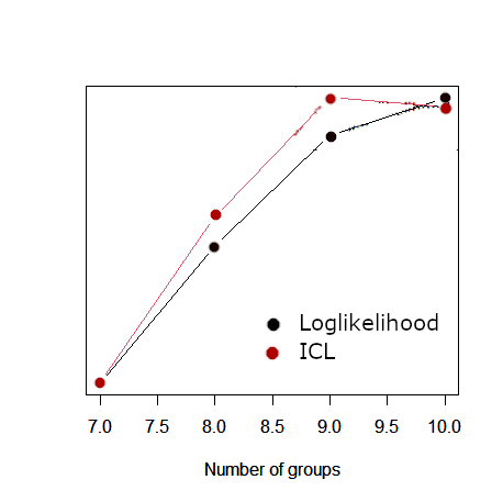
Figure 7: Integrated classification likelihood (ICL) and log-likelihood corresponding to different cluster numbers for French high school data.

We then compare the detected clusters from dynsbm with the actual class types in Table 9 at all the five time points.

Table 9: Clusters for French high school data by using the model in Matias and Miele, (2017).

	Detected clusters
Class types	0	1	2	3	4	5	6	7	8	9
$t=1$
BIO1	1	0	35	0	0	0	0	0	1	0
BIO2	1	0	0	0	0	1	0	0	31	0
BIO3	0	0	0	0	0	0	40	0	0	0
MP1	3	30	0	0	0	0	0	0	0	0
MP2	3	0	0	0	0	26	0	0	0	0
MP3	2	0	0	31	0	5	0	0	0	0
PC1	4	0	0	0	0	5	0	0	0	35
PC2	0	0	0	0	0	1	0	38	0	0
EGI	1	0	0	0	32	1	0	0	0	0
$t=2$
BIO1	0	0	36	0	0	0	0	0	1	0
BIO2	4	0	0	0	0	0	0	0	29	0
BIO3	1	0	0	0	0	0	39	0	0	0
MP1	0	31	0	0	0	2	0	0	0	0
MP2	2	0	0	0	0	27	0	0	0	0
MP3	1	0	0	34	0	3	0	0	0	0
PC1	3	0	0	0	0	2	0	0	0	39
PC2	3	0	0	0	0	1	0	35	0	0
EGI	3	0	0	0	31	0	0	0	0	0
$t=3$
BIO1	5	0	31	0	0	0	0	0	1	0
BIO2	2	0	0	0	0	0	0	0	31	0
BIO3	3	0	0	0	0	0	37	0	0	0
MP1	0	27	0	0	0	6	0	0	0	0
MP2	1	0	0	0	0	28	0	0	0	0
MP3	0	0	0	36	0	2	0	0	0	0
PC1	6	0	0	0	0	2	0	0	0	36
PC2	4	0	0	0	0	0	0	35	0	0
EGI	3	0	0	0	30	1	0	0	0	0
$t=4$
BIO1	2	0	35	0	0	0	0	0	0	0
BIO2	3	0	0	0	0	0	0	0	30	0
BIO3	7	0	0	0	0	0	33	0	0	0
MP1	1	28	0	0	0	4	0	0	0	0
MP2	1	1	0	0	0	27	0	0	0	0
MP3	4	0	0	34	0	0	0	0	0	0
PC1	4	0	0	0	0	3	0	0	0	37
PC2	4	0	0	0	0	0	0	35	0	0
EGI	6	0	0	0	26	2	0	0	0	0
$t=5$
BIO1	3	0	33	0	0	0	0	0	1	0
BIO2	2	0	0	0	0	0	0	0	31	0
BIO3	5	0	0	0	0	0	35	0	0	0
MP1	1	26	0	0	0	6	0	0	0	0
MP2	4	0	0	0	0	25	0	0	0	0
MP3	3	0	0	33	0	2	0	0	0	0
PC1	4	0	0	0	0	2	0	0	0	38
PC2	3	0	0	0	0	0	0	36	0	0
EGI	3	0	0	0	30	1	0	0	0	0

We may notice that dynsbm method reserves one group as “0” for subjects with no edges (the absence nodes). Our algorithm, in comparison, is not affected by those subjects.

Table 10: Detected clusters for the French high school data by using our method.

	Detected clusters
Class types	1	2	3	4	5	6	7	8	9
BIO1	0	0	1	0	0	0	0	0	36
BIO2	0	1	32	0	0	0	0	0	0
BIO3	0	1	0	0	39	0	0	0	0
MP1	33	0	0	0	0	0	0	0	0
MP2	0	1	0	28	0	0	0	0	0
MP3	0	0	0	0	0	38	0	0	0
PC1	0	44	0	0	0	0	0	0	0
PC2	0	0	0	0	0	0	0	39	0
EGI	0	0	0	0	0	0	34	0	0

The grouping results from dynsbm method is quite stable over the five time points. Such results lend support to our method which assumes the constant cluster structure over time. Furthermore, our clustering results, shown in Table 10, appear to be more accurate and agree more closely to the true grouping (class types) for this data analysis.

Another practical advantage of our method is its relatively short computing time. Using a computer with Intel(R) Core(TM) i7-10875H CPU and 32.0 GB RAM, we need to spend 0.36 and 252.39 seconds to obtain the community detection results with our method and dynsbm method, respectively.

B.2 Enron email data

The Enron email dataset contains approximately 500,000 emails generated by employees of the Enron Corporation. It was obtained by the Federal Energy Regulatory Commission during its investigation of Enron’s collapse. The data file was published at https://www.cs.cmu.edu/~./enron/.

Rastelli et al., (2017) developed a latent stochastic block model for directed dynamic network data. They applied their methods for the Enron email data. To compare with their results, we used data for all the emails exchanged from January 2000 to March 2002 ($n=27$) between the Enron members. The number of nodes in our analysis is $184$ (which is different from Rastelli et al., (2017) where they have kept $148$ subjects).

Using our spectral clustering algorithm for the whole network data and using the BIC, we obtain the best number of cluster is $13$. Rastelli et al., (2017) used the exact ICL criterion and found $17$ clusters but $4$ groups seem to be extremely small or just contain inactive nodes. Their algorithm is for directed graph and also assume time-varying membership. It seems our results are still quite close to Rastelli et al., (2017). Similar to their analysis, we can see that there is a high degree of heterogeneity with $13$ different clusters for this data set. When applying dynsbm package on this data the optimal number of cluster is only $6$.

Next we considered the change point analysis. Using our binary segmentation methods, we detect one change point at October 2001 which is exactly the month corresponding to the disclosure of Enron bankruptcy (see the log-likelihood functions plotted in Figure 8). This again agrees with the empirical findings in Rastelli et al., (2017).

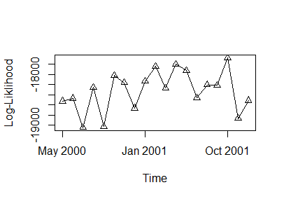
Figure 8: Log-likelihood functions corresponding to different change points in time for Enron email data.

References

• Aggarwal and Subbian, (2014) Aggarwal, C. and Subbian, K. (2014). Evolutionary network analysis: A survey. ACM Computing Surveys (CSUR), 47(1):1–36.
• Barbieri and Keshk, (2016) Barbieri, K. and Keshk, O. M. G. (2016). Correlates of War Project Trade Data Set Codebook, Version 4.0. Online: http://correlatesofwar.org.
• Barbieri et al., (2009) Barbieri, K., Keshk, O. M. G., and Pollins, B. (2009). Trading data: Evaluating our assumptions and coding rules. Conflict Management and Peace Science, 26(5):471–491.
• Bennett, (1962) Bennett, G. (1962). Probability inequalities for the sum of independent random variables. Journal of the American Statistical Association, 57(297):33–45.
• Bhattacharjee et al., (2020) Bhattacharjee, M., Banerjee, M., and Michailidis, G. (2020). Change point estimation in a dynamic stochastic block model. Journal of Machine Learning Research, 21(107):1–59.
• Bradley, (2007) Bradley, R. C. (2007). Introduction to strong mixing conditions. Kendrick press.
• (7) Chang, J., He, J., and Yao, Q. (2020a). Modelling matrix time series via a tensor cp-decomposition. Under preparation.
• (8) Chang, J., Kolaczyk, E. D., and Yao, Q. (2020b). Discussion of “network cross-validation by edge sampling”. Biometrika, 107(2):277–280.
• (9) Chang, J., Kolaczyk, E. D., and Yao, Q. (2020c). Estimation of subgraph densities in noisy networks. Journal of the American Statistical Association, (In press):1–40.
• Chen et al., (2020) Chen, E. Y., Fan, J., and Zhu, X. (2020). Community network auto-regression for high-dimensional time series. arXiv:2007.05521.
• Corneli et al., (2018) Corneli, M., Latouche, P., and Rossi, F. (2018). Multiple change points detection and clustering in dynamic networks. Statistics and Computing, 28(5):989–1007.
• Crane et al., (2016) Crane, H. et al. (2016). Dynamic random networks and their graph limits. The Annals of Applied Probability, 26(2):691–721.
• Donnat and Holmes, (2018) Donnat, C. and Holmes, S. (2018). Tracking network dynamics: A survey of distances and similarity metrics. The Annals of Applied Statistics, 12(2):971–1012.
• Durante et al., (2016) Durante, D., Dunson, D. B., et al. (2016). Locally adaptive dynamic networks. The Annals of Applied Statistics, 10(4):2203–2232.
• Durrett, (2019) Durrett, R. (2019). Probability: theory and examples, volume 49. Cambridge university press.
• Fan and Yao, (2003) Fan, J. and Yao, Q. (2003). Nonlinear Time Series: Nonparametric and Parametric Methods. Springer, New York.
• Friel et al., (2016) Friel, N., Rastelli, R., Wyse, J., and Raftery, A. (2016). Interlocking directorates in irish companies using a latent space model for bipartite networks. Proceedings of the national academy of sciences, 113(24):6629–6634.
• Fu et al., (2009) Fu, W., Song, L., and Xing, E. P. (2009). Dynamic mixed membership blockmodel for evolving networks. In Proceedings of the 26th Annual International Conference on Machine Learning, pages 329–336.
• Hanneke et al., (2010) Hanneke, S., Fu, W., and Xing, E. P. (2010). Discrete temporal models of social networks. Electronic Journal of Statistics, 4:585–605.
• Kang et al., (2017) Kang, X., Ganguly, A., and Kolaczyk, E. D. (2017). Dynamic networks with multi-scale temporal structure. arXiv preprint arXiv:1712.08586.
• Knight et al., (2016) Knight, M., Nunes, M., and Nason, G. (2016). Modelling, detrending and decorrelation of network time series. arXiv preprint arXiv:1603.03221.
• Kolaczyk, (2017) Kolaczyk, E. D. (2017). Topics at the Frontier of Statistics and Network Analysis. Cambridge University Press.
• Krivitsky and Handcock, (2014) Krivitsky, P. N. and Handcock, M. S. (2014). A separable model for dynamic networks. Journal of the Royal Statistical Society, B, 76(1):29.
• Lin and Bai, (2011) Lin, Z. and Bai, Z. (2011). Probability inequalities. Springer Science & Business Media.
• Ludkin et al., (2018) Ludkin, M., Eckley, I., and Neal, P. (2018). Dynamic stochastic block models: parameter estimation and detection of changes in community structure. Statistics and Computing, 28(6):1201–1213.
• Mastrandrea et al., (2015) Mastrandrea, R., Fournet, J., and Barrat, A. (2015). Contact patterns in a high school: A comparison between data collected using wearable sensors, contact diaries and friendship surveys. PLoS ONE, 10(9):e0136497.
• Matias and Miele, (2017) Matias, C. and Miele, V. (2017). Statistical clustering of temporal networks through a dynamic stochastic block model. Journal of the Royal Statistical Society, B, 79(4):1119–1141.
• Matias et al., (2018) Matias, C., Rebafka, T., and Villers, F. (2018). A semiparametric extension of the stochastic block model for longitudinal networks. Biometrika, 105(5):989–1007.
• Merlevède et al., (2009) Merlevède, F., Peligrad, M., Rio, E., et al. (2009). Bernstein inequality and moderate deviations under strong mixing conditions. In High dimensional probability V: the Luminy volume, pages 273–292. Institute of Mathematical Statistics.
• Pensky, (2019) Pensky, M. (2019). Dynamic network models and graphon estimation. Annals of Statistics, 47(4):2378–2403.
• Rastelli et al., (2017) Rastelli, R., Latouche, P., and Friel, N. (2017). Choosing the number of groups in a latent stochastic block model for dynamic networks. Online: http://arxiv.org/abs/1702.01418.
• Rohe et al., (2011) Rohe, K., Chatterjee, S., Yu, B., et al. (2011). Spectral clustering and the high-dimensional stochastic blockmodel. The Annals of Statistics, 39(4):1878–1915.
• Snijders, (2005) Snijders, T. A. B. (2005). Models for longitudinal network data. In Carrington, P., Scott, J., and Wasserman, S. S., editors, Models and Methods in Social Network Analysis, chapter 11. Cambridge University Press, New York.
• Vanhems et al., (2013) Vanhems, P., Barrat, A., Cattuto, C., Pinton, J.-F., Khanafer, N., Regis, C., a. Kim, B., and B. Comte, N. V. (2013). Estimating potential infection transmission routes in hospital wards using wearable proximity sensors. PloS ONE, 8:e73970.
• Vinh et al., (2010) Vinh, N. X., Epps, J., and Bailey, J. (2010). Information theoretic measures for clusterings comparison: Variants, properties, normalization and correction for chance. Journal of Machine Learning Research, 11:2837–2854.
• Wang et al., (2019) Wang, D., Liu, X., and Chen, R. (2019). Factor models for matrix-valued high-dimensional time series. Journal of Econometrics, 208(1):231–248.
• Wang et al., (2018) Wang, D., Yu, Y., and Rinaldo, A. (2018). Optimal change point detection and localization in sparse dynamic networks. arXiv preprint arXiv:1809.09602.
• Wilson et al., (2019) Wilson, J. D., Stevens, N. T., and Woodall, W. H. (2019). Modeling and detecting change in temporal networks via the degree corrected stochastic block model. Quality and Reliability Engineering International, 35(5):1363–1378.
• Xu and Hero, (2014) Xu, K. S. and Hero, A. O. (2014). Dynamic stochastic blockmodels for time-evolving social networks. IEEE Journal of Selected Topics in Signal Processing, 8(4):552–562.
• Yang et al., (2011) Yang, T., Chi, Y., Zhu, S., Gong, Y., and Jin, R. (2011). Detecting communities and their evolutions in dynamic social networks?a bayesian approach. Machine learning, 82(2):157–189.
• Yu et al., (2015) Yu, Y., Wang, T., and Samworth, R. J. (2015). A useful variant of the davis–kahan theorem for statisticians. Biometrika, 102(2):315–323.
• Yudovina et al., (2015) Yudovina, E., Banerjee, M., and Michailidis, G. (2015). Changepoint inference for erdös-rényi random graphs. In Stochastic Models, Statistics and Their Applications, pages 197–205. Springer.
• Zhao et al., (2019) Zhao, Z., Chen, L., and Lin, L. (2019). Change-point detection in dynamic networks via graphon estimation. arXiv preprint arXiv:1908.01823.
• (44) Zhu, T., Li, P., Yu, L., Chen, K., and Chen, Y. (2020a). Change point detection in dynamic networks based on community identification. IEEE Transactions on Network Science and Engineering.
• (45) Zhu, X., Huang, D., Pan, R., and Wang, H. (2020b). Multivariate spatial autoregressive model for large scale social networks. Journal of Econometrics, 215(2):591–606.
• Zhu et al., (2017) Zhu, X., Pan, R., Li, G., Liu, Y., and Wang, H. (2017). Network vector autoregression. The Annals of Statistics, 45(3):1096–1123.
• Zhu et al., (2019) Zhu, X., Wang, W., Wang, H., and Härdle, W. K. (2019). Network quantile autoregression. Journal of Econometrics, 212(1):345–358.