Causal inference for semi-competing risks data

Abstract

An emerging challenge for time-to-event data is studying semi-competing risks, namely when two event times are of interest: a non-terminal event time (e.g. age at disease diagnosis), and a terminal event time (e.g. age at death). The non-terminal event is observed only if it precedes the terminal event, which may occur before or after the non-terminal event. Studying treatment or intervention effects on the dual event times is complicated because for some units, the non-terminal event may occur under one treatment value but not under the other. Until recently, existing approaches (e.g., the survivor average causal effect) generally disregarded the time-to-event nature of both outcomes. More recent research focused on principal strata effects within time-varying populations under Bayesian approaches. In this paper, we propose alternative non time-varying estimands, based on a single stratification of the population. We present a novel assumption utilizing the time-to-event nature of the data, which is weaker than the often-invoked monotonicity assumption. We derive results on partial identifiability, suggest a sensitivity analysis approach, and give conditions under which full identification is possible. Finally, we present non-parametric and semi-parametric estimation methods for right-censored data.

Keywords: Illness-death model; principal stratification; survival analysis; non-parametric bounds; frailty model

1 Introduction

Semi-competing risks data arise when times to two events of interest are studied, non-terminal (e.g. disease diagnosis) and terminal (e.g. death) events. The non-terminal event is observed only if it precedes the terminal event, which may occur before or after the non-terminal event.

When the goal is to assess the causal effect of a treatment, exposure or an intervention on the two events, the effect on the terminal event only might not capture the scientific effect of interest. As a motivating example, consider the complex effect of having at least one Apolipoprotein E $\epsilon 4$ allele (APOE) on late-onset Alzheimer’s disease (AD) diagnosis (non-terminal event) and death (terminal event). APOE is a well-established risk factor for AD (Alzheimer’s Association, 2019). However, it is unknown whether APOE has a distinct causal effect on survival (Corder et al., 1993; Dal Forno et al., 2002; Wang et al., 2015), or even how to define this effect, due to its entanglement with AD, that by itself affects life expectancy. An observed APOE effect on death might be the result of a strong APOE effect on AD, and the occurrence of AD expedited the terminal event occurrence. An alternative explanation is that APOE affected death directly.

Problems also arise for the causal effect of APOE on AD (the non-terminal event). The standard average treatment effect is ill-defined because some study participants die without an AD diagnosis, leading to an infinite AD event time. Motivated by these challenges, this paper studies causal effects for semi-competing risks data, including their definition, non-parametric (partial) identification, estimation and inference about such effects.

Recent advancements in semi-competing risks data analysis often consider one of two main approaches, copula-based methods and the illness-death model. The copula-based approach focuses on the identifiable region of the joint survival function of the event times, namely the region in which the terminal event occurs after the non-terminal event (Fine et al., 2001). Then, a parametric copula function of the two marginal distributions is used to model the joint survival function on this region. While regression methods were also developed under this framework (Peng and Fine, 2007; Hsieh et al., 2008), to our knowledge, causal interpretation of this approach has not been studied. The illness-death model approach (Andersen et al., 1993) focuses on transition times between three different states: An initial state (state “0”, healthy), a diseased state (“1”, disease), and an absorbing state (“2”, death). Possible transitions are $0\rightarrow 1$, $0\rightarrow 2$ and $1\rightarrow 2$. Various specifications and time-to-event models have been suggested to analyze semi-competing risks data in this framework (Meira-Machado et al., 2006; Xu et al., 2010). Typically, inter-personal dependence between illness and death times is assumed to be captured by covariates, or modeled via a random effect, known as frailty (Xu et al., 2010; Lee et al., 2017; Gorfine et al., 2020).

In the causal inference paradigm, the related “truncation by death” problem has been studied (Zhang and Rubin, 2003; Hayden et al., 2005; Zhang et al., 2009; Long and Hudgens, 2013; Tchetgen Tchetgen, 2014; Ding and Lu, 2017). This problem arises when researchers aspire to compare outcomes (e.g. quality of life index) between the treated and untreated groups at a fixed time after the treatment was assigned, but some study participants have died prior to the outcome collection, hence the average causal effect is not well-defined. Using principal stratification (Frangakis and Rubin, 2002), the survivor average causal effect (SACE) is the causal effect within the stratum of people who would have survived under both treatment values. A similar problem arises in vaccination studies, where the effect of a vaccine on post-infection outcomes is well-defined only among those who would have been infected with or without vaccinating (Shepherd et al., 2007). Generally, the SACE is non-parametrically unidentifiable, unless strong assumptions are made (Hayden et al., 2005; Zhang et al., 2009). Therefore, researchers have developed bounds (Zhang and Rubin, 2003; Long and Hudgens, 2013) and sensitivity analyses (Hayden et al., 2005; Shepherd et al., 2007). However, none of these papers apply to semi-competing risks data, where the time-to-event nature of both disease diagnosis and survival times must be addressed.

Robins (1995) utilized additional assumptions to show the average causal effect (not SACE) is identifiable when censoring time is always observed, and without distinguishing between censoring due to death or other reasons. More recently, two papers have considered causal questions for semi-competing risks data (Comment et al., 2019; Xu et al., 2020). These papers suggested Bayesian methods to estimate the time-varying SACE (TV-SACE) and time-varying restricted mean survival time (RM-SACE). While these papers provide major improvement towards causal reasoning for semi-competing risks data, their proposed estimands can be hard to interpret, because at each time $t$ the population for which the time-varying estimands are defined is changing. Additionally, one of the works rely on parametric frailty-based illness-death models (Comment et al., 2019), while the other coupled a parametric sensitivity copula-based analysis with a non-parametric Bayesian method under an additional identifying assumption (Xu et al., 2020). Questions of non-parametric partial identifiability, including non-parametric bounds under weaker assumptions, or sensitivity analyses without the copula model, as well as frequentist non-parametric and semi-parametric estimation were all not addressed.

In this paper, we define new causal estimands for semi-competing risks data. The general idea resembles principal stratification in that we propose to stratify the population according to their potential outcomes. However, unlike the TV-SACE and RM-SACE, we focus on effects defined within a fixed, not time-varying, population. The contributions of our paper can be summarized as follows:

• New causal estimands for semi-competing risks data.

• Novel assumptions suitable for the semi-competing risks data structure. For example, our new assumption termed order preservation is weaker than the traditionally-used monotonicity assumption (Zhang and Rubin, 2003).

• Partial and full identifiability results for the proposed estimands.

• New tools for casual inference from semi-competing risks data that can be used in the presence of right censoring, a ubiquitous challenge in the analysis of time-to-event data. These include bounds, sensitivity analyses, non-parametric and semi-parametric estimators and inference methods.

• The R package CausalSemiComp implementing the developed methodology. Simulation results are fully reproducible. Both the package and reproducibility materials are available from the first author’s Github account.

2 Notation and causal estimands

Let $T_{1}(a)$ and $T_{2}(a)$ be the times to disease diagnosis and death, respectively, under treatment level $A=a$. Throughout the paper, we call $A$ a treatment, although in practice it could also be an exposure or an intervention. For example, $A=1$ may indicate having at least one APOE $\epsilon 4$ allele, while $A=0$ indicates no APOE $\epsilon$4 alleles. Then, $T_{1}(a)$ and $T_{2}(a)$ are the potential Alzheimer’s diagnosis and death times had we intervened on the APOE gene and set it to $A=a$.

The assumed probability space for $\{T_{1}(0),T_{2}(0),T_{1}(1),T_{2}(1)\}$ is as follows. Let $f_{a}(t_{1},t_{2})$ be the joint density function of $\{T_{1}(a),T_{2}(a)\}$ on $0<t_{1}\leq t_{2}$ for $a=0,1$. Because the terminal event may occur before the non-terminal event, precluding the observation of the latter, then $\Pr[T_{1}(a)<\infty]=\int_{0}^{\infty}\int_{0}^{t_{2}}f_{a}(t_{1},t_{2})dt_{1}dt_{2}<1$. The event $T_{1}(a)=\infty$ or, stated differently, $T_{1}(a)>T_{2}(a)$ corresponds to not having the non-terminal event under $A=a$. We defer assumptions on the joint distribution of $\{T_{1}(0),T_{2}(0)\}$ and $\{T_{1}(1),T_{2}(1)\}$ for later; these two pairs could never be observed simultaneously.

The causal inference perspective often focuses on contrasting averages of potential outcomes under different treatment levels. Consider the average causal effect of APOE on the survival time $E[T_{2}(1)-T_{2}(0)]$. Because APOE affects AD incidence (Alzheimer’s Association, 2019), and because AD patients are likely to die earlier compared to the scenario they did not have AD (Tom et al., 2015), we would expect $E[T_{2}(1)-T_{2}(0)]<0$, even if APOE does not carry an effect on age at death other than the effect resulting from earlier AD onset. Additionally, when focus is on the non-terminal event, $E[T_{1}(1)-T_{1}(0)]$ is ill-defined, because $T_{1}(a)=\infty$ for some study units for either or both $a=0$ and $a=1$.

Therefore, causal inference for semi-competing risks data is entangled. Principal stratification effects suggested to address this challenge are defined within a strata of the population created by the potential values of a post-randomization variable, which is not the object of inquiry (Frangakis and Rubin, 2002). For semi-competing risks, principal stratification approaches can be divided into two types: time-fixed and time-varying estimands. The time-fixed approach focuses on a single time point $\overline{t}$, say age 80, and define the binary potential outcomes $\mathcal{S}(a)=I\{T_{2}(a)>\overline{t}\}$ and $\mathcal{Y}(a)=I\{T_{1}(a)\leq\overline{t}\}$ as the survival status and Alzheimer’s status at time $\overline{t}$ under treatment level $A=a$. Then, the problem is posed as a truncation-by-death problem with the target causal estimand being the SACE: $E[\mathcal{Y}(1)-\mathcal{Y}(0)|\mathcal{S}(1)=\mathcal{S}(0)=1]$. The SACE compares the population-level risk of AD by age $\overline{t}$ with and without APOE only among those who would have survived until age $\overline{t}$ under both APOE statuses. Typically, strong assumptions are needed for identifying the SACE and researchers presented a variety of analyses under various assumptions. One commonly-made assumption is the monotonicity assumption $\mathcal{S}(1)\leq\mathcal{S}(0)$ (Zhang and Rubin, 2003; Ding et al., 2011; Ding and Lu, 2017). That is, those surviving beyond time $\overline{t}$ and have APOE would also survive beyond $\overline{t}$ had they did not have APOE. A more recent approach (Comment et al., 2019; Xu et al., 2020) focuses on the TV-SACE causal effect

$$TV\text{-}SACE(r,t)=\Pr[T_{1}(1)<r|T_{2}(1)>t,T_{2}(0)>t]-\Pr[T_{1}(0)<r|T_{2}(1)>t,T_{2}(0)>t]$$

for $r\leq t$. The $TV$-$SACE$ has two major advantages over the standard SACE: at each time $t$ it compares non-terminal event rates in multiple time points, and it respects that the population of always-survivors depends on the chosen time $t$. However, exactly because the population changes with time, it can be hard to interpret it as a function of $t$. A change in $TV$-$SACE(r,t)$ as a function of $t$ may reflect a change in the population or a change in efficacy of the treatment. Furthermore, that treatment effects cannot be summarized into a single number, even for a fixed $r$, might create a challenge in communicating the results to a broader audience.

2.1 Population stratification and alternative estimands

We propose alternative estimands, based on a single partition of the population. We divide the population into four strata according to their illness and death “order”. This partition resembles the principal stratification framework that typically stratifies the population according to a post-treatment variable which is not the outcome. Therefore, because our partition involves the dual outcomes, we term it population stratification. Define the following four subpopulations with respect to the order of $T_{1}(a),T_{2}(a)$ for $a=0,1$. The “always-diseased” ($ad$) will be diagnosed with the disease at some point of their life, regardless of their treatment status ($T_{1}(a)\leq T_{2}(a)$ for $a=0,1$); the “never-diseased” ($nd$) will die without having the disease first, regardless of their treatment status ($T_{1}(a)>T_{2}(a)$ for $a=0,1$); the “harmed” ($dh$) would be diagnosed with the disease prior to death only if treated ($T_{1}(0)>T_{2}(0),T_{1}(1)\leq T_{2}(1)$); and the “protected” ($dp$) would be diagnosed with the disease only if untreated ($T_{1}(0)\leq T_{2}(0),T_{1}(1)>T_{2}(1)$). Let $\pi_{ad}$, $\pi_{nd}$, $\pi_{dh}$ and $\pi_{dp}=1-\pi_{ad}-\pi_{nd}-\pi_{dh}$ be the respective subpopulation proportions; see also Table 1.

Table 1: Population stratification for semi-competing risks data.

Name	Stratum definition	Stratum proportion
Always-diseased (ad)	$T_{1}(0)\leq T_{2}(0)$ & $T_{1}(1)\leq T_{2}(1)$	$\pi_{ad}$
Never-diseased (nd)	$T_{1}(0)>T_{2}(0)$ & $T_{1}(1)>T_{2}(1)$	$\pi_{nd}$
Disease harmed (dh)	$T_{1}(0)>T_{2}(0)$ & $T_{1}(1)\leq T_{2}(1)$	$\pi_{dh}$
Disease protected (dp)	$T_{1}(0)\leq T_{2}(0)$ & $T_{1}(1)>T_{2}(1)$	$\pi_{dp}$

Because $T_{1}(a)=\infty$ for some $a$ for the $dh$ and $dp$ strata, well-defined causal effects that are of interest only exist within the $ad$ and the $nd$ strata, similar to cases where principal stratification has been utilized (Zhang and Rubin, 2003; Shepherd et al., 2007; Ding et al., 2011; Ding and Lu, 2017). In the motivating example (Section 6), the $ad$ and $nd$ proportions were estimated to be 35% and 53%, respectively, meaning nearly all the population belongs to a stratum within which there is a well-defined causal effect. At each time $t$, we can define the following causal estimands

$$\Pr [T_{2}(1)\leq t\ |\ ad]-\Pr[T_{2}(0)\leq t\ |\ ad],$$ (1)

$$\Pr [T_{2}(1)\leq t\ |\ nd]-\Pr[T_{2}(0)\leq t\ |\ nd],$$ (2)

$$\Pr [T_{1}(1)\leq t\ |\ ad]-\Pr[T_{1}(0)\leq t\ |\ ad].$$ (3)

Causal effects that better summarize the impact of $A$ could be based on the restricted mean survival time (RMST) (Chen and Tsiatis, 2001). For a given time point $t^{\star}$, let $\mathcal{T}_{j}(a)=\min[T_{j}(a),t^{\star}],a,j=0,1$, and define the following additional causal estimands

$$E [\mathcal{T}_{2}(1)-\mathcal{T}_{2}(0)\ |\ ad],$$ (4)

$$E [\mathcal{T}_{1}(1)-\mathcal{T}_{1}(0)\ |\ ad],$$ (5)

$$E \{[\mathcal{T}_{2}(1)-\mathcal{T}_{1}(1)]-[\mathcal{T}_{2}(0)-\mathcal{T}_{1}(0)]\ |\ ad\},$$ (6)

$$E [\mathcal{T}_{2}(1)-\mathcal{T}_{2}(0)\ |\ nd].$$ (7)

Each of these estimands characterizes a different causal effect of $A$ on the outcomes within the $ad$ or $nd$ stratum. Effects (4)–(6) are defined within $ad$. In the motivating example, effect (4) is the mean (possibly negative) gain in life expectancy caused by APOE, (5) is the effect of APOE on AD diagnosis age, and (6), which is obtained by subtracting (5) from (4), is the effect on the residual lifetime with AD. If, for example, the latter equals zero, it means the same life expectancy with AD is expected for those with and without APOE within the $ad$ stratum. Effect (7) is also of great interest, as it is the effect of APOE on life expectancy among the $nd$ population, thus it captures another form of APOE effect on survival. Furthermore, contrasting (4) with (7) may provide information on the heterogeneity of APOE effect on survival. Of course, other distribution summary measures (e.g. median time-to-events) can be used to define causal effects.

3 Identifiability

The focus of this section is on assumptions and identifiability. Methods for estimation and inference under right censoring are developed in Section 4. Let $(A,T_{1},T_{2})$ be the actual treatment and event times. Throughout this paper, we assume the following two standard assumptions (Hernan and Robins, 2019).

Assumption 1.

Stable Unit Treatment Value Assumption (SUTVA). $T_{1}=T_{1}(1)A+T_{1}(0)(1-A)$ and $T_{2}=T_{2}(1)A+T_{2}(0)(1-A)$.

Assumption 2.

Strong Ignorability, $A\mathchoice{\mathrel{\hbox to0.0pt{$\displaystyle\perp$\hss}\mkern 2.0mu{\displaystyle\perp}}}{\mathrel{\hbox to0.0pt{$\textstyle\perp$\hss}\mkern 2.0mu{\textstyle\perp}}}{\mathrel{\hbox to0.0pt{$\scriptstyle\perp$\hss}\mkern 2.0mu{\scriptstyle\perp}}}{\mathrel{\hbox to0.0pt{$\scriptscriptstyle\perp$\hss}\mkern 2.0mu{\scriptscriptstyle\perp}}}\{T_{1}(0),T_{2}(0)\},\{T_{1}(1),T_{2}(1)\}$.

In many observational studies that lack randomization, a conditional version of Assumption 2, conditionally on covariates, is more plausible.

3.1 Bounds

It is well-known that principal stratum effects are not identified from the data, unless additional assumptions are leveraged (Zhang et al., 2009; Ding et al., 2011; Tchetgen Tchetgen, 2014; Ding and Lu, 2017), and often bounds are developed (Zhang and Rubin, 2003; Long and Hudgens, 2013) . In this section, we present various bounds for the causal effects based on the identifiable distribution of $(A,T_{1},T_{2})$, constructed differently depending on the assumptions a researcher is willing to make. First, we present a new assumption, tailored for semi-competing risks data.

Assumption 3.

Order preservation. If $T_{1}(0)\leq T_{2}(0)$, then $T_{1}(1)\leq T_{2}(1)$.

In the motivating example, under Assumption 3 anyone who would have been diagnosed with AD without having APOE, would also have AD had they had APOE, but not necessarily at the same age. It is consistent with the overwhelming evidence that APOE significantly increases the risk of AD (Alzheimer’s Association, 2019). Assumption 3 can be easily modified for studies with a beneficing effect of $A$ on the non-terminal event time.

Assumption 3 is less restrictive than the often-invoked monotonicity assumption (Zhang and Rubin, 2003; Long and Hudgens, 2013). Unlike monotonicity, Assumption 3 acknowledges the realistic scenario that $A$ may impact survival time for either direction. Specifically, it allows that $T_{2}(0)-T_{2}(1)$ and $T_{1}(0)-T_{1}(1)$ are of different signs at the unit level. To see this, observe that $T_{1}(1)\leq T_{2}(1)$ implies $T_{2}(0)-T_{2}(1)\leq[T_{2}(0)-T_{1}(0)]+[T_{1}(0)-T_{1}(1)]$. Finally, Assumption 3 implies that the $dp$ stratum is empty, i.e., $\pi_{dp}=0$.

As is typically the case in truncation-by-death problems, even under Assumptions 1–3, none of the causal effects (1)–(7) are non-parametrically identifiable from the data. These effects are however partially identifiable, in the sense that the data, coupled with the assumptions, provide bounds on these effects. For any event $\mathcal{Q}$, let $F_{j|\mathcal{Q}}(t)=\Pr(T_{j}\leq t|\mathcal{Q})$, $S_{j|\mathcal{Q}}(t)=1-F_{j|\mathcal{Q}}(t)$ and $\eta_{\mathcal{Q}}=\Pr(T_{1}\leq T_{2}|\mathcal{Q})$. Under Assumptions 1–3, $\Pr(T_{2}(0)\leq t\ |\ ad),\Pr(T_{2}(1)\leq t\ |\ nd)$ and $\Pr(T_{1}(0)\leq t\ |\ ad)$ are identified from the data, while $\Pr(T_{2}(1)\leq t\ |\ ad),\Pr(T_{2}(0)\leq t\ |\ nd)$ and $\Pr(T_{1}(1)\leq t\ |\ ad)$ are only partially identified. The following proposition establishes partial identifiability under Assumptions 1–3.

Proposition 1.

Under Assumptions 1–3, effects (1)–(3) are partially identified by

$$\mathcal{L}_{2,ad}(t)\leq\Pr[T_{2}(1)\leq t|ad]-\Pr[T_{2}(0)\leq t|ad]\leq\mathcal{U}_{2,ad}(t),$$ (8)

$$\mathcal{L}_{2,nd}(t)\leq\Pr[T_{2}(1)\leq t|nd]-\Pr[T_{2}(0)\leq t|nd]\leq\mathcal{U}_{2,nd}(t),$$ (9)

$$\mathcal{L}_{1,ad}(t)\leq\Pr[T_{1}(1)\leq t|ad]-\Pr[T_{1}(0)\leq t|ad]\leq\mathcal{U}_{1,ad}(t),$$ (10)

where

$$\begin{split}&\mathcal{L}_{2,ad}(t)=\max\left\{0\ ,1-\frac{S_{2|A=1}(t)}{\eta_{A=0}}\right\}-F_{2|A=0,T_{1}\leq T_{2}}(t),\\ &\mathcal{U}_{2,ad}(t)=\min\left\{1\ ,F_{2|A=1}(t)\frac{\eta_{A=1,T_{2}\leq t}}{\eta_{A=0}}\right\}-F_{2|A=0,T_{1}\leq T_{2}}(t),\\ &\mathcal{L}_{2,nd}(t)=F_{2|A=1,T_{1}>T_{2}}(t)-\min\left\{1\ ,F_{2|A=0}(t)\frac{1-\eta_{A=0,T_{2}\leq t}}{1-\eta_{A=1}}\right\},\\ &\mathcal{U}_{2,nd}(t)=F_{2|A=1,T_{1}>T_{2}}(t)-\max\left\{0\ ,1-\frac{S_{2|A=0}(t)}{1-\eta_{A=1}}\right\},\\ &\mathcal{L}_{1,ad}(t)=\max\left\{0\ ,1-\frac{S_{1|A=1}(t)}{\eta_{A=0}}\right\}-F_{1|A=0,T_{1}\leq T_{2}}(t),\\ &\mathcal{U}_{1,ad}(t)=\min\left\{1\ ,\frac{F_{1|A=1}(t)}{\eta_{A=0}}\right\}-F_{1|A=0,T_{1}\leq T_{2}}(t).\end{split}$$ (11)

The proof is given in Section A.1 of the Supplementary Materials (SM). From the proof it could also be seen that under Assumptions 1–3, the strata proportions are identified by $\pi_{ad}=\eta_{A=0}$, $\pi_{dh}=\eta_{A=1}-\eta_{A=0}$, $\pi_{nd}=1-\eta_{A=1}$. Since $T_{1}(a)$ and $T_{2}(a)$ are positive with probability one, RMST effects (5)–(7) are (partially) identified by recalling that for any non-negative random variable, $E(T)=\int_{0}^{\infty}[1-\Pr(T\leq t)]dt$.

Proposition 1 provides bounds for the different causal effects. Had we had unlimited data, calculating the bounds would have been simple. In the absence of right censoring, we could have simply calculate $F_{2|A=a}(t),F_{2|A=a,T_{1}\leq T_{2}}(t)$, $\eta_{A=a},\eta_{A=a,T_{2}\leq t}$ from the data. As for $F_{1|A=a}(t)$, we could have used $F_{1|A=a}(t)=\eta_{A=a}F_{1|A=a,T_{1}\leq T_{2}}(t)$.

Generally, bounds derived under additional assumptions may provide narrower bounds (Zhang and Rubin, 2003; Long and Hudgens, 2013). Of course, these assumptions need to be plausible in the scientific problem at hand for the bounds to be valid. One particular bound that may not be informative enough is $\mathcal{L}_{1,ad}(t)$. As $t$ increases, the second term $F_{1|A=0,T_{1}\leq T_{2}}(t)$ get closer to one while the first term is not, because $\Pr(T_{1}<\infty|{A=1})<1$. As a remedy for this problem, consider the following assumption and proposition providing a more informative lower bound for (3).

Assumption 4.

For a given $t$, $\Pr[T_{1}(1)\leq t|ad]\geq\Pr[T_{1}(1)\leq t|dh]$.

This assumption resembles the ranked average score assumption (Zhang and Rubin, 2003), but tailored for time-to-event data. It means that the probability of an always-diseased person to be diagnosed with the disease by time $t$ (under $A=1$) is larger than the probability of same event for a disease-harmed person (also under $A=1$). In practice, Assumption 4 can hold for some, all, or none of the values of $t$. It will hold if those in the $ad$ stratum tend to be diagnosed at earlier ages than those in the $dh$ stratum.

Proposition 2.

Under Assumptions 1–3, for any $t$ for which Assumption 4 holds, $\Pr[T_{1}(1)\leq t|ad]-\Pr[T_{1}(0)\leq t|ad]$ is partially identified by

$$\widetilde{\mathcal{L}}_{1,ad}(t)\leq\Pr[T_{1}(1)\leq t|ad]-\Pr[T_{1}(0)\leq t|ad]\leq\mathcal{U}_{1,ad}(t)$$

where $\widetilde{\mathcal{L}}_{1,ad}(t)=F_{1|A=1T_{1}\leq T_{2}}(t)-F_{1|A=0,T_{1}\leq T_{2}}(t)$ and $\mathcal{U}_{1,ad}(t)$ is given in Proposition 1.

The proof is given in Section A.2 of the SM. In some studies, the obtained bounds, with or without additional assumptions, might be too wide to have practical utility. One approach is to improve the bounds by leveraging an additional covariate. Following Long and Hudgens (2013), we develop below narrower bounds utilizing a pre-intervention discrete covariate $Z$. In the motivating example, $Z$ can be, for example, gender. An adjusted version of Proposition 1 can be obtained under the following assumption.

Assumption 5.

$A\mathchoice{\mathrel{\hbox to0.0pt{$\displaystyle\perp$\hss}\mkern 2.0mu{\displaystyle\perp}}}{\mathrel{\hbox to0.0pt{$\textstyle\perp$\hss}\mkern 2.0mu{\textstyle\perp}}}{\mathrel{\hbox to0.0pt{$\scriptstyle\perp$\hss}\mkern 2.0mu{\scriptstyle\perp}}}{\mathrel{\hbox to0.0pt{$\scriptscriptstyle\perp$\hss}\mkern 2.0mu{\scriptscriptstyle\perp}}}Z,\{T_{1}(0),T_{2}(0)\},\{T_{1}(1),T_{2}(1)\}$.

For example, we show in Section A.3 of the SM that under Assumptions 1, 3 and 5, adjusted bounds for (1) are given by $\mathcal{L}^{Z}_{2,ad}(t),\mathcal{U}^{Z}_{2,ad}(t)$, where

$$\begin{split}&\mathcal{L}^{Z}_{2,ad}(t)=\sum_{z}\nu(z)\left[\max\left\{0\ ,1-\frac{S_{2|A=1,Z=z}(t)}{\eta_{A=0,Z=z}}\right\}-F_{2|A=0,T_{1}\leq T_{2},Z=z}(t)\right],\\ &\mathcal{U}^{Z}_{2,ad}(t)=\sum_{z}\nu(z)\left[\min\left\{1\ ,F_{2|A=1,Z=z}(t)\frac{\eta_{A=1,T_{2}\leq t,Z=z}}{\eta_{A=0,Z=z}}\right\}-F_{2|A=0,T_{1}\leq T_{2},Z=z}(t)\right],\end{split}$$ (12)

and $\nu(z)=\Pr(Z=z|A=0,T_{1}\leq T_{2})$. Furthermore, the following proposition establishes that the adjusted bounds are always within the unadjusted bounds.

Proposition 3.

Under Assumptions 1, 3 and 5, $\mathcal{L}_{2,ad}(t)\leq\mathcal{L}^{Z}_{2,ad}(t)$ and $\mathcal{U}_{2,ad}(t)\geq\mathcal{U}^{Z}_{2,ad}(t)$.

The proof is given in Section A.4 of the SM. Proposition 3 is the analogue of Proposition 1 in Long and Hudgens (2013), who developed bounds when the outcome is binary, and also investigated under which conditions the statement in the inequalities can be made in the sharp sense. Of note is that due to finite-sample variation, Proposition 3 may not hold empirically. Therefore, as suggested by Long and Hudgens (2013), the bounds $\max\{\mathcal{L}_{2,ad}(t),\mathcal{L}^{Z}_{2,ad}(t)\}$ and $\min\{\mathcal{U}_{2,ad}(t),\mathcal{U}^{Z}_{2,ad}(t)\}$ can be used.

We summarize this section by an illustrative comparison of the various bounds. Figure 1 presents the bounds for three scenarios; the data-generating mechanism (DGM) and the resulting per-stratum cumulative distribution functions are described in Section D.1 of the SM. Under Scenario (I) (top row), Assumptions 3 and 4 hold, and $A=1$ shorten the $ad$ time-to-disease and time-to-death, and $nd$ die faster under $A=1$. The bounds $\{\mathcal{L}_{1,ad}(t),\mathcal{U}_{1,ad}(t)\}$, $\{\mathcal{L}_{2,ad}(t),\mathcal{U}_{2,ad}(t)\}$, and $\{\mathcal{L}_{2,nd}(t),\mathcal{U}_{2,nd}(t)\}$ (in pink shade) are quite wide in this scenario. The bound $\widetilde{\mathcal{L}}_{1,ad}(t)$ (dashed green line), derived in Proposition 2 is far more informative, being only slightly lower than the true difference (black solid curve). The adjusted bounds (blue dotted lines) were narrower than the unadjusted bounds, most notably for $t$ values for which the unadjusted bounds are very wide. For the causal effect on time-to-disease within the $ad$ (top left corner) the narrower bound is obtained as $\{\widetilde{\mathcal{L}}_{1,ad}(t),\mathcal{U}^{Z}_{2,ad}(t)\}$. The bounds for time-to-death among the $nd$ are quite wide. This is likely because there is least information on this group from the observed data, as the true strata probability were $(\pi_{ad},\pi_{nd},\pi_{dh})=(0.49,0.15,0.36)$.

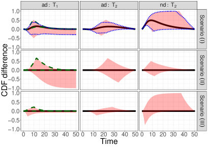
Figure 1: True causal effects (1)–(3) and different bounds under three simulated scenarios.

To further investigate this point, consider the second and third rows of Figure 1, both under null effects with no covariate $Z$ available. In Scenario (II), the $nd$ stratum comprised most of the population $(\pi_{ad},\pi_{nd},\pi_{dh})=(0.13,0.59,0.28)$ and the bounds were quite narrow for the within $nd$ effect $\eqref{Eq:estimand:ProbT2nd}$, and less informative for the $ad$. In Scenario (III), when $\pi_{ad}$ was substantial $(\pi_{ad},\pi_{nd},\pi_{dh})=(0.70,0.07,0.23)$, the bounds were quite narrow for the within $ad$ causal effects $\eqref{Eq:estimand:ProbT2ad}$ and $\eqref{Eq:estimand:ProbT1ad}$, but not so informative for the $nd$ stratum. In conclusion, if the proportion of one of the stratum $ad$ or $nd$ is large enough, the bounds can be useful, and a covariate $Z$ may help to make the bounds narrower. If Assumption 4 is plausible, the lower bound $\widetilde{\mathcal{L}}_{1,ad}(t)$ can be quite informative.

A covariate that can be used to sharpen the bounds is not always available, or even if it is, the bounds might still be too wide. Therefore, alternative strategies for an analysis are desirable. In Section B of the SM we describe a sensitivity analysis approach arising from the proof of Proposition 1. However, our main approach towards conducting sensitivity analysis for casual effect estimation from semi-competing risks data stems from the ubiquitous illness-death modeling of semi-competing risks data.

3.2 Identification by frailty assumptions

We turn to present stronger assumptions under which effects (1)–(3) are identified from the data. The proposed overarching strategy adapts the illness-death model so causal estimands can be captured by the model, by formulating two illness-death models and tying them together via a bivariate frailty random variable $\boldsymbol{\gamma}=(\gamma_{0},\gamma_{1})$. For $a=0,1$, let

$$\lambda_{01}(t|a,\boldsymbol{\gamma}) =\lim\limits_{\Delta\rightarrow 0}\Delta^{-1}\Pr[T_{1}\in[t,t+\Delta)|A=a,T_{1}\geq t,T_{2}\geq t,\boldsymbol{\gamma}],\quad t>0,$$

$$\lambda_{02}(t|a,\boldsymbol{\gamma}) =\lim\limits_{\Delta\rightarrow 0}\Delta^{-1}\Pr[T_{2}\in[t,t+\Delta)|A=a,T_{1}\geq t,T_{2}\geq t,\boldsymbol{\gamma}],\quad t>0,$$

$$\lambda_{12}(t|a,t_{1},\boldsymbol{\gamma}) =\lim\limits_{\Delta\rightarrow 0}\Delta^{-1}\Pr[T_{2}\in[t,t+\Delta)|A=a,T_{1}=t_{1},T_{2}\geq t,\boldsymbol{\gamma}],\quad t>t_{1}>0$$

be the three cause-specific hazard functions under the semi-competing risks setting (Xu et al., 2010), associated with the transitions $j\rightarrow k,jk=01,02,12$ (0: healthy, 1: disease, 2: death); see Figure C.1 in the SM for illustration. Our approach requires assumptions on the conditional (in)dependence of $\{T_{1}(0),T_{2}(0)\}$ and $\{T_{1}(1),T_{2}(1)\}$ given $\boldsymbol{\gamma}$.

Assumption 6.

There exists a bivariate random variable $\boldsymbol{\gamma}=(\gamma_{0},\gamma_{1})$ such that

1. Given $\boldsymbol{\gamma}$, the joint distribution of the potential event times can be factored as follows

   $$f[T_{1}(0),T_{2}(0),T_{1}(1),T_{2}(1)|\boldsymbol{\gamma}]=f[T_{1}(0),T_{2}(0)|\gamma_{0}]f[T_{1}(1),T_{2}(1)|\gamma_{1}],$$ (13)

   where $f(\cdot)$ denotes a density function of a possibly-multivariate random variable.

2. $A\mathchoice{\mathrel{\hbox to0.0pt{$\displaystyle\perp$\hss}\mkern 2.0mu{\displaystyle\perp}}}{\mathrel{\hbox to0.0pt{$\textstyle\perp$\hss}\mkern 2.0mu{\textstyle\perp}}}{\mathrel{\hbox to0.0pt{$\scriptstyle\perp$\hss}\mkern 2.0mu{\scriptstyle\perp}}}{\mathrel{\hbox to0.0pt{$\scriptscriptstyle\perp$\hss}\mkern 2.0mu{\scriptscriptstyle\perp}}}\{T_{1}(0),T_{2}(0),\gamma_{0}\},\{T_{1}(1),T_{2}(1),\gamma_{1}\}$.

3. The frailty variable operates multiplicatively on the hazard functions. That is, $\lambda_{jk}(t|a,\boldsymbol{\gamma})=\gamma_{a}\widetilde{\lambda}_{jk}(t|a)$ for $jk=01,02,a=0,1$ and $\lambda_{12}(t|a,t_{1},\boldsymbol{\gamma})=\gamma_{a}\widetilde{\lambda}_{12}(t|a,t_{1})$ for $a=0,1$, for some $\widetilde{\lambda}_{jk}$ functions.

4. The probability density function of $\boldsymbol{\gamma}$, $f_{\boldsymbol{\theta}}(\boldsymbol{\gamma})$, is known up to a finite dimensional parameter $\boldsymbol{\theta}$ that is identifiable from the observed data distribution.

Part $(i)$ of Assumption 6 implies a cross-world independence conditionally on the unobserved $\boldsymbol{\gamma}$. This assumption is more general than Assumption 4 in Comment et al. (2019) in that their assumption additionally assumes $\gamma_{0}=\gamma_{1}$. However, $\gamma_{0}=\gamma_{1}$ would generally not hold unless all treatment effect modifiers can be measured and correctly accounted for via changes in the $\widetilde{\lambda}_{jk}$ functions between $a=0$ and $a=1$. Part $(ii)$ is just an adaption of Assumption 2 for the frailty case and $(iii)$ and $(iv)$ are standard assumptions for identification of the observed data distribution. The strategy of how to model the distribution of $\boldsymbol{\gamma}$ dictates two forms of dependence, cross-world and within-world. We give below three examples of frailty distributions specifications.

Example 1.

A bivariate normal distribution with mean zero and a given correlation $\rho$ is assumed for $[\log(\gamma_{1}),\log(\gamma_{2})]$. The variances $Var(\log{\gamma_{a}})$ are identifiable from the data.

Example 2.

The frailty variables $(\gamma_{0},\gamma_{1})$ are independent Gamma random variables, with mean one and variances $\theta_{0}$ and $\theta_{1}$, respectively, both identifiable from the data.

Example 3.

The frailty variables are $(\gamma_{0},\gamma_{1})$ correlated Gamma variables, with mean one, variances $\theta_{0}$ and $\theta_{1}$, and correlation $\rho$. The frailty variances $\theta_{0}$ and $\theta_{1}$ are identifiable from the data, while $\rho$ is unidentifiable and need to be supplied by the researcher.

Crucially, Example 3 entails a weaker assumption than assuming that $\gamma_{0}=\gamma_{1}$. The latter implies the same dependence between the non-terminal and terminal event times in both worlds. Thus, it constraints the effect of $A$ on $\{T_{1},T_{2}\}$, and hence it constitutes a strong assumption, that should not hold at least in some settings. Assumption 6, especially its first part, is generally a strong assumption. Nevertheless, it opens the way for causal interpretation of existing semi-competing risks models.

Proposition 4.

Under Assumptions 1 and 6, the causal effects (1)–(3) are identified by

$$\Pr [T_{2}(1)\leq t|ad]-\Pr[T_{2}(0)\leq t|ad]$$

$$=\int_{0}^{\infty}\int_{0}^{\infty}[F_{2|T_{1}\leq T_{2},A=1,\gamma_{1}}(t)-F_{2|T_{1}\leq T_{2},A=0,\gamma_{0}}(t)\}]\frac{\eta_{A=0,\gamma_{0}}\eta_{A=1,\gamma_{1}}f_{\boldsymbol{\theta}}(\boldsymbol{\gamma})d\boldsymbol{\gamma}}{\int_{0}^{\infty}\int_{0}^{\infty}\eta_{A=0,\gamma^{\prime}_{0}}\eta_{A=1,\gamma^{\prime}_{1}}f_{\boldsymbol{\theta}}(\boldsymbol{\gamma}^{\prime})d\boldsymbol{\gamma}^{\prime}},$$

$$\Pr [T_{2}(1)\leq t|nd]-\Pr[T_{2}(0)\leq t|nd]$$

$$=\int_{0}^{\infty}\int_{0}^{\infty}[F_{2|T_{1}>T_{2},A=1,\gamma_{1}}(t)-F_{2|T_{1}>T_{2},A=0,\gamma_{0}}(t)]\frac{(1-\eta_{A=0,\gamma_{0}})(1-\eta_{A=1,\gamma_{1}})f_{\boldsymbol{\theta}}(\boldsymbol{\gamma})d\boldsymbol{\gamma}}{\int_{0}^{\infty}\int_{0}^{\infty}(1-\eta_{A=0,\gamma^{\prime}_{0}})(1-\eta_{A=1,\gamma^{\prime}_{1}})f_{\boldsymbol{\theta}}(\boldsymbol{\gamma}^{\prime})d\boldsymbol{\gamma}^{\prime}},$$

$$\Pr [T_{1}(1)\leq t|ad]-\Pr[T_{1}(0)\leq t|ad]$$

$$=\int_{0}^{\infty}\int_{0}^{\infty}[F_{1|T_{1}\leq T_{2},A=1,\gamma_{1}}(t)-F_{1|T_{1}\leq T_{2},A=0,\gamma_{0}}(t)\}]\frac{\eta_{A=0,\gamma_{0}}\eta_{A=1,\gamma_{1}}f_{\boldsymbol{\theta}}(\boldsymbol{\gamma})d\boldsymbol{\gamma}}{\int_{0}^{\infty}\int_{0}^{\infty}\eta_{A=0,\gamma^{\prime}_{0}}\eta_{A=1,\gamma^{\prime}_{1}}f_{\boldsymbol{\theta}}(\boldsymbol{\gamma}^{\prime})d\boldsymbol{\gamma}^{\prime}},$$

where for any event $\mathcal{Q}$, $F_{j|\mathcal{Q},\boldsymbol{\gamma}}(t)=\Pr(T_{j}\leq t|\mathcal{Q},\boldsymbol{\gamma})$. Furthermore, all the integrals can be consistently estimated from the data.

The proof is given in Section A.5 of the SM. RMST-like estimands (5)–(7) are identified by suitable integration over $t$. A sensitivity analyses based on Proposition 4 can be carried out by repeating the analysis (e.g. under Example 3) for different $\rho$ values.

Regarding the choice of which frailty distribution to use in practice, it is well-known that misspecification of the frailty distribution leads to only small bias in the estimated cumulative incidence function, integrated over the frailty distribution; see Gorfine et al. (2020) and references therein.

Figure 2 illustrates the causal RMST effects (4), (5), and (7) under the DGM described in Section 4 and Section D.1 of the SM, and the frailty specification given in Example 3, with equal variances $\theta=\theta_{0}=\theta_{1}$. Stratum proportions varied between 41%–45% for $ad$ stratum and 8%–12% for the $nd$ stratum. The causal RMST effects, calculated at $t^{\star}=15$, were sensitive to $\rho$ when the stratum proportion was very small and the frailty variance was large, and were otherwise quite robust to $\rho$.

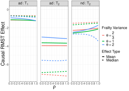
Figure 2: Causal mean and median RMST effects as a function of the frailty variance $\theta=\theta_{0}=\theta_{1}=2/3,1,2$, (corresponding to Kendall’s $\tau=1/4,1/3,1/2$) and correlation between the frailty variables $\rho\in[0,1]$. RMST effects were calculated at $t^{\star}=15$.

3.3 Right censoring

Time-to-event outcome data are often not fully observed for all individuals due to loss to follow-up (i.e., right censoring). Two issues arise when considering right censoring. The first is identification of the causal estimand, considered in this section, and the second is how to estimate the different quantities and provide inference, which is embedded in the non-parametric and semi-parametric methods presented in Section 4. Let $C(a)$ be the censoring time under $A=a$. We first adjust Assumption 2 for the case of censoring.

Assumption 7.

Strong Ignorability $A\mathchoice{\mathrel{\hbox to0.0pt{$\displaystyle\perp$\hss}\mkern 2.0mu{\displaystyle\perp}}}{\mathrel{\hbox to0.0pt{$\textstyle\perp$\hss}\mkern 2.0mu{\textstyle\perp}}}{\mathrel{\hbox to0.0pt{$\scriptstyle\perp$\hss}\mkern 2.0mu{\scriptstyle\perp}}}{\mathrel{\hbox to0.0pt{$\scriptscriptstyle\perp$\hss}\mkern 2.0mu{\scriptscriptstyle\perp}}}\{T_{1}(0),T_{2}(0),C(0)\},\{T_{1}(1),T_{2}(1),C(1)\}$.

Our next assumption is a within-world independent-censoring assumption.

Assumption 8.

Independent censoring $\{T_{1}(a),T_{2}(a)\}\mathchoice{\mathrel{\hbox to0.0pt{$\displaystyle\perp$\hss}\mkern 2.0mu{\displaystyle\perp}}}{\mathrel{\hbox to0.0pt{$\textstyle\perp$\hss}\mkern 2.0mu{\textstyle\perp}}}{\mathrel{\hbox to0.0pt{$\scriptstyle\perp$\hss}\mkern 2.0mu{\scriptstyle\perp}}}{\mathrel{\hbox to0.0pt{$\scriptscriptstyle\perp$\hss}\mkern 2.0mu{\scriptscriptstyle\perp}}}C(a)$ for $a=0,1$.

Assumption 8 asserts that, under each treatment value, the two event times and censoring time are independent. We also assume the standard assumption that there exists an end of follow-up time $\overline{c}$ and that $Pr(T_{j}(a)>\overline{c})>0$ for $j=1,2$. Combining Assumptions 7 and 8 together with Assumption 1, we get the standard independent censoring assumption for semi-competing risks data $T_{1},T_{2}\mathchoice{\mathrel{\hbox to0.0pt{$\displaystyle\perp$\hss}\mkern 2.0mu{\displaystyle\perp}}}{\mathrel{\hbox to0.0pt{$\textstyle\perp$\hss}\mkern 2.0mu{\textstyle\perp}}}{\mathrel{\hbox to0.0pt{$\scriptstyle\perp$\hss}\mkern 2.0mu{\scriptstyle\perp}}}{\mathrel{\hbox to0.0pt{$\scriptscriptstyle\perp$\hss}\mkern 2.0mu{\scriptscriptstyle\perp}}}C$, with $C$ being the censoring time under $A$.

3.4 Covariates inclusion

There are number of reasons to include baseline covariates $\boldsymbol{X}$ in our setting. First, because in observational studies the intervention is not randomized, Assumption 7 is more plausible when made conditionally on $\boldsymbol{X}$. Second, the independent censoring assumption (Assumption 8) is also more plausible when made conditionally on $\boldsymbol{X}$ (Andersen et al., 1993). Assumption 6 is also more plausible when made conditionally on covariates. For simplicity of presentation, we use the same vector $\boldsymbol{X}$ for all assumptions to hold. In Section A.6 of the SM, we adapt Propositions 1 and 4 to include covariates. An additional reason to include covariates is to improve estimators’ efficiency. In the motivating example (Section 6), we use gender and race as covariates. Note that the role of $\boldsymbol{X}$ is different from the role of the covariate $Z$ we utilized in Section 3.1.

While a variety of statistical models have been used for semi-competing risks data, how to elucidate information on causal effects is typically overlooked and, in practice, researchers often focus on specific coefficients in regression models. Therefore, a main motivation for us to consider models is to enable translation of existing model results into knowledge on the causal effects of interest. Comment et al. (2019) used parametric models coupled with Bayesian methods for estimating the TV-SACE and RM-SACE. We focus on frequentist estimation of and inference about causal effects (4)–(7) under semi-parametric frailty models that align with Assumption 6. Details are given in Section 4.2.

4 Estimation and Inference

So far, our focus has been on definitions of causal estimands, assumptions and their plausibility, and identification strategies. We now turn to estimation of the identifiable components based on time-to-event right-censored semi-competing risks data, and carrying out inference for these quantities. We first propose non-parametric estimators and discuss their asymptotic properties, before considering semi-parametric models. For the non-parametric estimators, our efforts are focused on the quantities $\eta_{A=a}$, $\eta_{A=a,T_{2}\leq t}$, $S_{1|A=a}$, $S_{2|A=a}$, $S_{1|A=a,T_{1}\leq T_{2}}$, $S_{2|A=a,T_{1}\leq T_{2}}$, and $S_{2|A=a,T_{1}>T_{2}}$ (for $a=0,1$). These are the building blocks of the bounds. For the semi-parametric estimation, we focus on a frailty proportional hazard model that allows estimation of causal effects utilizing Proposition 4.

For each participant $i$, $i=1,...,n$ denote by $Z_{i}$ a covariate that may be used for obtaining sharper bounds (when available), by $\boldsymbol{X}_{i}$ a vector of baseline covariates (when available), by $A_{i}\in\{0,1\}$, the intervention value, and by $T_{ij}$ the non-terminal ($j=1$) and terminal ($j=2$) event times. Let also $C_{i}$ be the censoring time. The observed data for each unit is $(Z_{i},\boldsymbol{X}_{i},A_{i},\widetilde{T}_{i1},\delta_{i1},\widetilde{T}_{i2},\delta_{i2})$ where $\widetilde{T}_{i1}=\min(T_{i1},T_{i2},C_{i})$ and $\widetilde{T}_{i2}=\min(T_{i2},C_{i})$ are the observed times, and $\delta_{i1}=I\{\widetilde{T}_{i1}=T_{i1}\}$ and $\delta_{i2}=I\{\widetilde{T}_{i2}=T_{i2}\}$ are the event indicators of disease and death, respectively. Let also $Y_{ij}(t)=I\{t\leq\widetilde{T}_{ij}\}$ be the at-risk processes.

4.1 Non-parametric Estimation

Starting with $S_{2|A=a}(t)$, it can be simply estimated by the Kaplan-Meier (KM) estimator of $T_{2}$ within the $\{A=a\}$ group. Regarding $S_{1|A=a}(t)$, observe that

$$S_{1|A=a}(t)=Pr(T_{1}>t|A=a)=-\int_{0}^{\infty}S_{1|A=a,T_{2}=s}[\min(t,s)]dS_{2|A=a}(s),$$ (14)

because for $t>s$, $S_{1|A=a,T_{2}=s}(t)=S_{1|A=a,T_{2}=s}(s)$, i.e., among those who die at time $s$, no new disease cases are possible later than $s$. The function $S_{1|A=a,T_{2}=t}$ is well-defined, and thus can be estimated non-parametrically. An explicit model for $S_{1|A=a,T_{2}=t}$ is of little interest, as it is hard to motivate a model for the nonstandard distribution of $T_{1}|T_{2}=t$.

We propose to estimate $S_{1|A=a,T_{2}=t}(t)$ by a kernel-smoothed KM estimator (Beran, 1981) within the $\{A=a,\delta_{2}=1\}$ group. Estimation among this group is valid because under Assumption 8, $S_{1|A=a,T_{2}=t}(t)=S_{1|A=a,T_{2}=t,\delta_{2}=1}(t)$. Let $K(\cdot)$ be a kernel function ($K(t)\geq 0$, $\int K(t)dt=1$), and let $h_{n}\rightarrow 0$ be a sequence of bandwidths. In practice, one might consider a separate bandwidth for each treatment level. For simplicity of presentation, we assume $h_{n}$ is the same for both $a=0,1$. Let $Q(t,a;h_{n})=\sum_{i=1}^{n}I\{A_{i}=a\}\delta_{i2}K[(t-T_{i2})/h_{n}]$, and $W_{i}(t,a;h_{n})=I\{A_{i}=a\}\delta_{i2}K[(t-T_{i2})/h_{n}]/Q(t,a;h_{n})$. The kernel KM estimator for $S_{1|A=a,T_{2}=t}(t)$ is then defined by

$$\widehat{S}_{1|A=a,T_{2}=t}(t)=\prod_{i=1}^{n}\left[1-\frac{W_{i}(t,a;h_{n})}{\sum_{j=1}^{n}Y_{1j}(\widetilde{T}_{i1})W_{j}(t,a;h_{n})}\right]^{\delta_{i1}\delta_{i2}I\{A_{i}=a,\widetilde{T}_{i1}\leq t\}}.$$

We propose to estimate $\eta_{A=a}$ in similar fashion utilizing that

$$\begin{split}\eta_{A=a}=Pr(T_{1}\leq T_{2}|A=a)=-\int_{0}^{\infty}F_{1|A=a,T_{2}=t}(t)dS_{2|A=a}(t).\end{split}$$ (15)

Turning to the other components, by calculations given in Section C.1 of the SM,

$$\eta_{A=a,T_{2}\leq t} =-\frac{1}{F_{2|A=a}(t)}\int_{0}^{t}F_{1|A=a,T_{2}=s}(s)dS_{2|A=a}(s),$$ (16)

$$S_{1|A=a,T_{1}\leq T_{2}}(t) =-\frac{1}{\eta_{A=a}}\int_{t}^{\infty}[S_{1|A=a,T_{2}=s}(t)-S_{1|A=a,T_{2}=s}(s)]dS_{2|A=a}(s),$$ (17)

$$S_{2|A=a,T_{1}\leq T_{2}}(t) =1-\frac{\eta_{A=a,T_{2}\leq t}F_{2|A=a}}{\eta_{A=a}},$$ (18)

$$S_{2|A=a,T_{1}>T_{2}}(t) =1-\frac{(1-\eta_{A=a,T_{2}\leq t})F_{2|A=a}}{1-\eta_{A=a}}.$$ (19)

Thus, estimators $\widehat{S}_{1|A=a}(t)$, $\widehat{\eta}_{A=a}$, $\widehat{\eta}_{A=a,T_{2}\leq t}$, $\widehat{S}_{2|A=a,T_{1}\leq T_{2}}(t)$ and $\widehat{S}_{2|A=a,T_{1}>T_{2}}(t)$, are obtained by substituting the KM and smoothed KM estimators into (14)–(19). Covariate-adjusted bounds (LABEL:Eq:AdjustedBound) are estimated at each level of $Z$, and then averaged using $\widehat{\nu}(z)=\widehat{\Pr}(Z=z)\widehat{\eta}_{Z=z}/\widehat{\Pr}(T_{1}\leq T_{2})$. Note, because the estimators are risk-set based, they accommodate not only right censoring but also delayed entry, as we illustrate in Section 6. Our R package CausalSemiComp implements methodology presented in this Section utilizing the prodlim package (Gerds, 2019) for calculating the smoothed KM estimators.

The asymptotic properties of the KM estimator and of the smoothed KM estimator are well established. For example, under Assumption 8 and additional regularity assumptions, the smoothed KM estimator is consistent and weakly converges to a Gaussian process (Beran, 1981; Dabrowska, 1987). A sketch of the proof of the consistency of our proposed estimators is provided in Section C.2 of the SM.

4.2 Semi-parametric frailty models

Under Assumption 6, we propose to use the following proportional hazard specification for the hazard functions of the six processes

$$\begin{split}\lambda_{01}(t|a,\boldsymbol{X},\gamma)&=\gamma_{a}\lambda_{01}^{0}(t|a)\exp(\boldsymbol{X}^{T}\boldsymbol{\beta}_{01}^{a})\,\,\,,t>0\\ \lambda_{02}(t|a,\boldsymbol{X},\gamma)&=\gamma_{a}\lambda_{02}^{0}(t|a)\exp(\boldsymbol{X}^{T}\boldsymbol{\beta}_{02}^{a})\,\,\,,t>0\\ \lambda_{12}(t|t_{1},a,\boldsymbol{X},\gamma)&=\gamma_{a}\lambda_{12}^{0}(t|a)\exp(\boldsymbol{X}^{T}\boldsymbol{\beta}_{12}^{a})\,\,\,,t>t_{1}>0\,,\end{split}$$ (20)

where $\lambda_{jk}^{0}(t|a),jk=01,02,12,a=0,1$ are unspecified baseline hazard functions. Define also the cumulative baseline hazard functions, $\Lambda_{jk}^{0}(t|a)=\int_{0}^{t}\lambda_{jk}^{0}(u|a)du$, and let $\boldsymbol{\beta}=(\boldsymbol{\beta}_{01}^{0T},\boldsymbol{\beta}_{02}^{0T},\boldsymbol{\beta}_{12}^{0T},\boldsymbol{\beta}_{01}^{1T},\boldsymbol{\beta}_{02}^{1T},\boldsymbol{\beta}_{12}^{1T})^{T}$, and $\boldsymbol{\Lambda}_{0}=(\Lambda_{01}^{0}(t|a),\Lambda_{02}^{0}(t|a),\Lambda_{12}^{0}(t|a))$ for $a=0,1$. Finally, let $\boldsymbol{\psi}=(\boldsymbol{\Lambda}_{0},\boldsymbol{\beta},\boldsymbol{\theta})$ be the collection of parameters to be estimated from the data. Assuming the data was prospectively collected with participants being disease-free at study starting time, it can be shown that the likelihood function (Xu et al., 2010) is proportional to

$$\mathcal{L}(\boldsymbol{\psi})= \prod_{i=1}^{n}\Bigg{\{}[\lambda_{01}^{0}(\widetilde{T}_{i1}|A_{i})]^{\delta_{i1}}[\lambda_{02}^{0}(\widetilde{T}_{i1}|A_{i})]^{(1-\delta_{i1})\delta_{i2}}[\lambda_{12}^{0,A_{i}}(\widetilde{T}_{i2}|A_{i})]^{\delta_{i1}\delta_{i2}}$$ (21)

$$\exp \bigg{[}\delta_{i1}\boldsymbol{X}_{i}^{T}\boldsymbol{\beta}^{A_{i}}_{01}+(1-\delta_{i1})\delta_{i2}\boldsymbol{X}_{i}^{T}\boldsymbol{\beta}^{A_{i}}_{02}+\delta_{i1}\delta_{i2}\boldsymbol{X}_{i}^{T}\boldsymbol{\beta}^{A_{i}}_{12}\bigg{]}(-1)^{\delta_{i1}+\delta_{i2}}\phi_{A_{i}}^{(\delta_{i1}+\delta_{i2})}(s_{i})\Bigg{\}},$$

where $\phi_{a}(s)=E\left\{\exp\{-s\gamma_{a}\}\right\}$ is the Laplace transform of $\gamma_{a}$, $a=0,1$, and $\phi_{a}^{(q)}$ is the $q$th derivative of $\phi_{a}(s)$ with respect to $s$, $q=0,1,2$, and

$$s_{i}=\sum_{j=1}^{2}\exp(\boldsymbol{X}_{i}^{T}\boldsymbol{\beta}_{0j}^{A_{i}})\Lambda_{0j}^{0}(\widetilde{T}_{i1}|A_{i})+\delta_{i1}\exp(\boldsymbol{X}_{i}^{T}\boldsymbol{\beta}_{12}^{A_{i}})\big{[}\Lambda_{12}^{0}(\widetilde{T}_{i2}|A_{i})-\Lambda_{12}^{0}(\widetilde{T}_{i1}|A_{i})\big{]}.$$

For the likelihood derivation see SM3 of Gorfine et al. (2020). We propose to utilize an EM algorithm for maximizing (21); the details are given in Section C.3 of the SM. The algorithm is implemented by our R package CausalSemiComp. Importantly, the estimation phase ignores the unidentifiable component $Cor(\gamma_{0},\gamma_{1})$ while estimating model (20) parameters. Assumptions on the joint distribution of $(\gamma_{0},\gamma_{1})$ are used to map the estimator $\hat{\boldsymbol{\psi}}$ into estimates of causal effects. Upon estimating $\hat{\boldsymbol{\psi}}$, the quantities in the identifying formulas from Proposition 4 can be calculated by numerical integration or Monte Carlo simulations, as we do below in Section 5.2.

5 Simulations

To assess the finite-sample properties of the proposed estimators, we conducted simulations under various scenarios with 1,000 simulation iterations per scenario. Sample size was $n=2,000$ and different censoring rates were considered. The DGM initially followed (20) with Weibull baseline hazards, two covariates, and Gamma frailty as described in Example 3 of Section 3.2 with $\theta_{0}=\theta_{1}$ for simplicity. Treatment was randomized with $\Pr(A=1)=0.5$. Further details on the different DGMs, analyses and results are presented in Section D of the SM.

5.1 Non-parametric estimation

We considered the scenarios previously used in Figure 3. Assumption 3 was imposed by re-simulating those initially at the $dh$ stratum. For the smoothed KM estimator, we used the default choices of the prodlim package (Gerds, 2019). Standard errors were estimated by bootstrap (sampling at the unit level) with 100 repetitions.

The estimators of $\eta_{A=a}$, $S_{1|A=a}(10)$ and $S_{1|A=a}(30)$ (Table 2) showed negligible empirical bias, the standard errors were well estimated and the 95% Wald-type confidence intervals had satisfactory empirical coverage rate. Under moderate censoring, an expected increase in the standard errors was observed. Section D.3 of the SM presents results for Scenario (III) and for additional parameters.

Table 2: Performance of the proposed non-parametric estimators. Censoring rates considered were low (10%, C-L) and moderate (30%, C-M). True: True parameter values; Mean.EST: mean estimate; EMP.SD: empirical standard deviation of the estimates; EST.SE: mean estimated standard error; CP95%: empirical coverage rate of 95% confidence interval.

	$\eta_{A=0}$		$\eta_{A=1}$		$S_{1|A=0}(10)$		$S_{1|A=0}(30)$		$S_{1|A=1}(10)$		$S_{1|A=1}(30)$
	C-L	C-M	C-L	C-M	C-L	C-M	C-L	C-M	C-L	C-M	C-L	C-M
Scenario (I)
True	0.491		0.848		0.748		0.523		0.481		0.158
Mean.EST	0.491	0.492	0.845	0.844	0.749	0.748	0.524	0.523	0.479	0.476	0.159	0.159
EMP.SD	0.016	0.020	0.011	0.012	0.014	0.016	0.016	0.020	0.017	0.019	0.012	0.012
EST.SE	0.017	0.019	0.011	0.012	0.014	0.017	0.017	0.019	0.017	0.019	0.011	0.012
CP95%	0.946	0.944	0.951	0.948	0.950	0.949	0.945	0.940	0.953	0.942	0.944	0.951
Scenario (II)
True	0.144		0.431		0.968		0.867		0.604		0.158
Mean.EST	0.146	0.145	0.429	0.426	0.968	0.967	0.865	0.866	0.904	0.903	0.601	0.599
EMP.SD	0.012	0.015	0.016	0.018	0.006	0.007	0.012	0.014	0.010	0.012	0.016	0.019
EST.SE	0.012	0.015	0.016	0.019	0.006	0.007	0.012	0.015	0.010	0.013	0.016	0.019
CP95%	0.945	0.946	0.938	0.937	0.939	0.942	0.943	0.949	0.953	0.956	0.945	0.941

5.2 Semi-parametric estimation

In this simulation study, the data was generated under under model (20) and was not restricted to follow Assumption 3. Frailties were simulated according to Example 3, with $\rho=0.5$ and equal variances $\theta=2/3,1,2$, corresponding to Kendall’s $\tau=1/4,1/3,1/2$ between $T_{1}(a)$ and $T_{2}(a)$. For each simulated dataset, we fitted two illness-death frailty models for $A=0,1$ using the EM algorithm (Section C.3 of the SM). Frailty variances were estimated separately and then combined (see Section D.2.2 of the SM). RMST causal effects were estimated by a Monte Carlo integration together with the estimated baseline hazards $\widehat{\boldsymbol{\Lambda}}$, coefficients $\widehat{\boldsymbol{\beta}}$ and $\widehat{\theta}$. This Monte Carlo procedure is described in length in Section D.2 of the SM. Standard errors were estimated using bootstrap with 100 repetitions.

Generally, the empirical bias of the estimated mean and median RMST effects was relatively negligible, standard errors were well estimated, and coverage provabilities were satisfactory (Table 3). The regression coefficients, baseline hazard functions and frailty variance were all also well estimated (Section D.3 of the SM). We repeated the simulation studies for $\rho=0,1$ (Section D.3 of the SM); the results did not change qualitatively.

Table 3: Performance of the semi-parametric estimators under Scenario (IV) with $\rho=0.5$, under low (5%, C-L) and moderate (25%, C-M) censoring rates for $T_{2}$. Censoring rates for $T_{1}$ were 35-40%. The presented effects are (5), (4) and (7) (ATE) and their median versions (MTE). True: True parameter values; Mean.EST: mean estimate; EMP.SD: empirical standard deviation of the estimates; EST.SE: mean estimated standard error; CP95%: empirical coverage rate of 95% confidence interval.

	$T_{1}|ad$				$T_{2}|ad$				$T_{2}|nd$
	ATE		MTE		ATE		MTE		ATE		MTE
	C-L	C-M	C-L	C-M	C-L	C-M	C-L	C-M	C-L	C-M	C-L	C-M
$\theta=2/3$
True	-1.16		-0.67		-3.95		-7.17		-2.18		-1.44
Mean.EST	-1.20	-1.21	-0.68	-0.68	-3.94	-3.95	-6.96	-6.93	-2.18	-2.18	-1.45	-1.45
EMP.SD	0.19	0.19	0.18	0.18	0.39	0.42	0.65	0.72	0.27	0.30	0.23	0.25
EST.SE	0.18	0.19	0.18	0.19	0.40	0.43	0.65	0.72	0.27	0.29	0.24	0.25
CP95%	0.94	0.94	0.94	0.95	0.95	0.95	0.96	0.93	0.95	0.93	0.95	0.94
$\theta=1$
True	-1.15		-0.71		-3.65		-6.83		-2.42		-1.58
Mean.EST	-1.20	-1.20	-0.73	-0.73	-3.66	-3.68	-6.72	-6.69	-2.42	-2.44	-1.59	-1.61
EMP.SD	0.20	0.22	0.19	0.20	0.42	0.45	0.58	0.64	0.32	0.35	0.26	0.27
EST.SE	0.20	0.22	0.20	0.21	0.41	0.45	0.61	0.67	0.34	0.36	0.27	0.28
CP95%	0.96	0.93	0.96	0.95	0.93	0.95	0.98	0.97	0.96	0.95	0.96	0.95
$\theta=2$
True	-1.01		-0.78		-3.09		-5.60		-2.23		-2.71
Mean.EST	-1.02	-1.04	-0.78	-0.80	-3.07	-3.06	-5.59	-5.55	-2.31	-2.30	-2.78	-2.74
EMP.SD	0.25	0.26	0.25	0.25	0.42	0.47	0.67	0.71	0.48	0.51	0.51	0.54
EST.SE	0.25	0.27	0.25	0.26	0.44	0.46	0.69	0.74	0.48	0.54	0.54	0.58
CP95%	0.95	0.96	0.94	0.95	0.95	0.94	0.95	0.95	0.95	0.96	0.96	0.96

6 Illustrative data analysis

The Adult Changes in Thought (ACT) Study is an ongoing prospective cohort study focused on dementia in the elderly. Starting from 1994, Alzheimer’s-free participants of age 65 and older from the Seattle metropolitan area have been recruited. More details can be found elsewhere (Kukull et al., 2002; Nevo et al., 2020). Here, $A=1$ means having at least one APOE $\epsilon 4$ allele. Excluding post-intervention variables, our analyses also include the binary variables gender and race (white/non-white). This leaves us with 4,453 participants, of which 1,783 (40%) were censored prior to either event, 211 (5%) were diagnosed with AD and then censored, 1,635 (37%) died without an AD diagnosis, and 824 (19%) were diagnosed with AD and died during follow-up.

Figure 3 presents the estimated bounds for causal effects (1)–(3) under Assumption 3 (in pink shade), utilizing gender as an additional covariate (in blue) and under the additional Assumption 4 (in green, for (3) only). Both Assumptions 3 and 4 seem reasonably plausible in this application, because it is well-established that APOE is a strong predictor of AD. The $ad$ proportion $\pi_{ad}$ was estimated to be 35% (CI95: 32%, 37%). The bounds $[\widetilde{\mathcal{L}}_{1,ad}(t),\mathcal{U}^{Z}_{2,ad}(t)]$ (bottom green and top blue) demonstrate that APOE induces earlier AD onset within the $ad$ stratum. The bounds do not allow for definite conclusions regarding the effect of APOE on death, and the inclusion of the variable gender had only minor effect. Focusing on the $nd$ stratum, its proportion was estimated to be 53% (CI95: 49%, 58%), meaning the two stratum of interest together comprise the vast majority of the population. Whether APOE had a positive or negative effect on survival in the $nd$ is unclear, although the lower bound was larger than zero for early ages.

In the semi-parametric analysis under Assumption 6 and Example 3, two illness-death models (20) were fitted using the EM algorithm, and included gender and race as covariates $\boldsymbol{X}$ (see SM Table E.14 for the estimated coefficients). Because participants in the ACT were recruited in varying ages, data was left truncated. We followed the approximation of Nielsen et al. (1992), by replacing all risk indicators $I\{t\leq\widetilde{T}_{ij}\}$ with $I\{R_{i}\leq t\leq\widetilde{T}_{ij}\}$, where $R_{i}$ is the age at recruitment. Estimated Gamma frailty variances were $\hat{\theta}_{0}=0.047,\hat{\theta}_{1}=0.027$ and then combined for simplicity of Monte Carlo estimation of casual effects. The estimated frailty variance was $\hat{\theta}=0.042$ (SE: $0.005$), corresponding to Kendall’s $\tau$ of 0.02. Turning to causal effects (Table 4), significant long-term negative effects of APOE on AD onset within the $ad$ stratum were estimated; those with APOE are expected to receive an AD diagnosis approximately 2 years earlier. Additionally, death at earlier age was expected in both strata under APOE. For $t^{\star}=15$ (age 80), effects were zero for the $nd$ stratum and negative though small for the $ad$. For $t^{\star}=25,35$ (ages 90,100), effects were negative in both strata, but stronger for the $ad$. The estimated effects did not change substantially as a function of $\rho$, as expected in low frailty variance scenarios (recall Figure 2).

To summarize the findings, APOE was found to expedite AD development within the $ad$ stratum. APOE was shown to have harmful effect on long-term age at death in both strata only under Assumption 6 and the semi-parametric modeling.

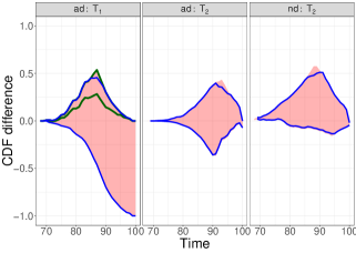
Figure 3: Bounds for principal effects of APOE on AD and death based on the ACT data. In pink shade the simple bounds, in blue bounds adjusted for gender and in green bounds based on Assumption 4.

Table 4: Estimated RMST causal effects of APOE on AD and death times within the $ad$ and $nd$ strata. Effects presented are mean (ATE) and median (MTE) differences. Results presented for $\rho=0.5$. The empirical distribution of gender and race in the data was used for calculating RMST effects.

		AD		Death
Stratum	$t^{\star}$	$\widehat{ATE}$ (95% CI)	$\widehat{MTE}$ (95% CI)	$\widehat{ATE}$ (95% CI)	$\widehat{MTE}$ (95% CI)
$ad$	$15$	-0.04 (-0.12, 0.04)	0.00 (-0.07, -0.52)	-0.61 (-0.70, -0.05)	-1.00 (-1.09, 0.08)
	$25$	-1.28 (-1.35, -1.20)	-2.00 (-2.07, -2.43)	-2.52 (-2.61, -0.48)	-3.00 (-3.08, -0.92)
	$35$	-1.82 (-1.89, -1.74)	-2.01 (-2.09, -2.35)	-2.42 (-2.5, -1.67)	-3.00 (-3.07, -1.90)
$nd$	$15$			-0.13 (-0.22, 0.07)	0.00 (-0.08, -0.91)
	$25$			-0.56 (-0.65, -1.92)	-1.00 (-1.08, -2.92)
	$35$			-1.75 (-1.84, -1.92)	-1.99 (-2.08, -2.93)

7 Discussion

It has been increasingly acknowledged that considering dual outcomes may provide more information about the scientific problem in hand, especially in the presence of death as a competing risk. In time-to-event data analysis, the semi-competing risks framework allows for consideration of dual outcomes. However, while methods have been developed for studying such data, questions of causality were only recently began to be studied (Comment et al., 2019; Xu et al., 2020).

We proposed new estimands built upon a population stratification approach, and discussed their partial and full identifiability, under variety of assumptions. The utility of the proposed approach is largest when either the never-diseased or the always-diseased strata comprise many of the population members. As demonstrated in Section 3, in these cases the partial identification is sharper for the population-stratified effects. This paper established an approach to study causal effects for semi-competing risks data, and discussed both the theory it hinges on and its practical use. Ultimately, we believe this will strengthen semi-competing risks data analysis, giving clear guidelines to what causal analyses should be carried out and under which assumptions causal conclusion can be derived.

References

- Alzheimer’s Association (2019) Alzheimer’s Association (2019). 2019 Alzheimer’s disease facts and figures. Alzheimer’s & Dementia 15(3), 321 – 387.
- Andersen et al. (1993) Andersen, P. K., O. Borgan, R. D. Gill, and N. Keiding (1993). Statistical models based on counting processes. New York: Springer-Verlag.
- Beran (1981) Beran, R. (1981). Nonparametric regression with randomly censored survival data.
- Chen and Tsiatis (2001) Chen, P.-Y. and A. A. Tsiatis (2001). Causal inference on the difference of the restricted mean lifetime between two groups. Biometrics 57(4), 1030–1038.
- Comment et al. (2019) Comment, L., F. Mealli, S. Haneuse, and C. Zigler (2019). Survivor average causal effects for continuous time: a principal stratification approach to causal inference with semicompeting risks. arXiv preprint arXiv:1902.09304.
- Corder et al. (1993) Corder, E., A. Saunders, W. Strittmatter, D. Schmechel, P. C. Gaskell, G. Small, A. Roses, J. Haines, and M. Pericak-Vance (1993). Gene dose of Apolipoprotein E type 4 allele and the risk of Alzheimer’s disease in late onset families. Science 261(5123), 921–923.
- Dabrowska (1987) Dabrowska, D. M. (1987). Non-parametric regression with censored survival time data. Scandinavian Journal of Statistics, 181–197.
- Dal Forno et al. (2002) Dal Forno, G., K. Carson, R. Brookmeyer, J. Troncoso, C. Kawas, and J. Brandt (2002). APOE genotype and survival in men and women with Alzheimer’s disease. Neurology 58(7), 1045–1050.
- Ding et al. (2011) Ding, P., Z. Geng, W. Yan, and X.-H. Zhou (2011). Identifiability and estimation of causal effects by principal stratification with outcomes truncated by death. Journal of the American Statistical Association 106(496), 1578–1591.
- Ding and Lu (2017) Ding, P. and J. Lu (2017). Principal stratification analysis using principal scores. Journal of the Royal Statistical Society: Series B (Statistical Methodology) 79(3), 757–777.
- Fine et al. (2001) Fine, J. P., H. Jiang, and R. Chappell (2001). On semi-competing risks data. Biometrika 88(4), 907–919.
- Frangakis and Rubin (2002) Frangakis, C. E. and D. B. Rubin (2002). Principal stratification in causal inference. Biometrics 58(1), 21–29.
- Gerds (2019) Gerds, T. A. (2019). prodlim: Product-Limit Estimation for Censored Event History Analysis. R package version 2019.11.13.
- Gorfine et al. (2020) Gorfine, M., N. Keret, A. B. Arie, D. Zucker, and L. Hsu (2020). Marginalized Frailty-Based Illness-Death Model: Application to the UK-Biobank Survival Data. Journal of the American Statistical Association, DOI 10.1080/01621459.2020.1831922.
- Hayden et al. (2005) Hayden, D., D. K. Pauler, and D. Schoenfeld (2005). An estimator for treatment comparisons among survivors in randomized trials. Biometrics 61(1), 305–310.
- Hernan and Robins (2019) Hernan, M. A. and J. M. Robins (2019). Causal inference. CRC Boca Raton, FL.
- Hsieh et al. (2008) Hsieh, J.-J., W. Wang, and A. A. Ding (2008). Regression analysis based on semicompeting risks data. Journal of the Royal Statistical Society: Series B (Statistical Methodology) 70(1), 3–20.
- Kukull et al. (2002) Kukull, W., R. Higdon, J. Bowen, W. McCormick, L. Teri, G. Schellenberg, G. van Belle, L. Jolley, and E. Larson (2002). Dementia and Alzheimer disease incidence: a prospective cohort study. Arch of Neurology 59(11), 1737–1746.
- Lee et al. (2017) Lee, K. H., V. Rondeau, and S. Haneuse (2017). Accelerated failure time models for semi-competing risks data in the presence of complex censoring. Biometrics 73(4), 1401–1412.
- Long and Hudgens (2013) Long, D. M. and M. G. Hudgens (2013). Sharpening bounds on principal effects with covariates. Biometrics 69(4), 812–819.
- Meira-Machado et al. (2006) Meira-Machado, L., J. De Una-Alvarez, and C. Cadarso-Suarez (2006). Nonparametric estimation of transition probabilities in a non-markov illness–death model. Lifetime Data Analysis 12(3), 325–344.
- Nevo et al. (2020) Nevo, D., D. Blacker, E. B. Larson, and S. Haneuse (2020). Modeling semi-competing risks data as a longitudinal bivariate process. arXiv preprint arXiv:2007.04037.
- Nielsen et al. (1992) Nielsen, G. G., R. D. Gill, P. K. Andersen, and T. I. Sørensen (1992). A counting process approach to maximum likelihood estimation in frailty models. Scandinavian journal of Statistics, 25–43.
- Peng and Fine (2007) Peng, L. and J. P. Fine (2007). Regression modeling of semicompeting risks data. Biometrics 63(1), 96–108.
- Robins (1995) Robins, J. M. (1995). An analytic method for randomized trials with informative censoring: part 1. Lifetime Data Analysis 1(3), 241–254.
- Shepherd et al. (2007) Shepherd, B. E., P. B. Gilbert, and T. Lumley (2007). Sensitivity analyses comparing time-to-event outcomes existing only in a subset selected postrandomization. Journal of the American Statistical Association 102(478), 573–582.
- Tchetgen Tchetgen (2014) Tchetgen Tchetgen, E. J. (2014). Identification and estimation of survivor average causal effects. Statistics in medicine 33(21), 3601–3628.
- Tom et al. (2015) Tom, S. E., R. A. Hubbard, P. K. Crane, S. J. Haneuse, J. Bowen, W. C. McCormick, S. McCurry, and E. B. Larson (2015). Characterization of dementia and alzheimer’s disease in an older population: updated incidence and life expectancy with and without dementia. American journal of public health 105(2), 408–413.
- Wang et al. (2015) Wang, X., O. Lopez, R. A. Sweet, J. T. Becker, S. T. DeKosky, M. M. Barmada, E. Feingold, F. Y. Demirci, and M. I. Kamboh (2015). Genetic determinants of survival in patients with Alzheimer’s disease. Journal of Alzheimer’s Disease 45(2), 651–658.
- Xu et al. (2010) Xu, J., J. D. Kalbfleisch, and B. Tai (2010). Statistical analysis of illness–death processes and semicompeting risks data. Biometrics 66(3), 716–725.
- Xu et al. (2020) Xu, Y., D. Scharfstein, P. Müller, and M. Daniels (2020). A Bayesian nonparametric approach for evaluating the causal effect of treatment in randomized trials with semi-competing risks. Biostatistics.
- Zhang and Rubin (2003) Zhang, J. L. and D. B. Rubin (2003). Estimation of causal effects via principal stratification when some outcomes are truncated by “death”. Journal of Educational and Behavioral Statistics 28(4), 353–368.
- Zhang et al. (2009) Zhang, J. L., D. B. Rubin, and F. Mealli (2009). Likelihood-based analysis of causal effects of job-training programs using principal stratification. Journal of the American Statistical Association 104(485), 166–176.