Lyapunov-stable orientation estimator for humanoid robots

Abstract

In this paper, we present an observation scheme, with proven Lyapunov stability, for estimating a humanoid’s floating base orientation. The idea is to use velocity aided attitude estimation, which requires to know the velocity of the system. This velocity can be obtained by taking into account the kinematic data provided by contact information with the environment and using the IMU and joint encoders. We demonstrate how this operation can be used in the case of a fixed or a moving contact, allowing it to be employed for locomotion. We show how to use this velocity estimation within a selected two-stage state tilt estimator: (i) the first which has a global and quick convergence (ii) and the second which has smooth and robust dynamics. We provide new specific proofs of almost global Lyapunov asymptotic stability and local exponential convergence for this observer. Finally, we assess its performance by employing a comparative simulation and by using it within a closed-loop stabilization scheme for HRP-5P and HRP-2KAI robots performing whole-body kinematic tasks and locomotion.

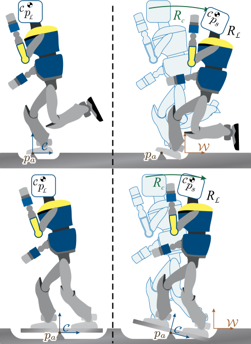
Figure 1: Model of the anchor point definition in the case of non fixed anchor. In the top an example of single support phase and in the bottom a double support. The origin of the control frame $\mathcal{C}$ is located at the position of the anchor point. The origin of the world frame $\mathcal{W}$ can be located anywhere. The rotation $R_{\mathcal{C}}$ between the world frame $\mathcal{W}$ and the control frame $\mathcal{C}$ is not available with encoders.

I Introduction

A humanoid robot is a system that is intended to move through the environment. However, this robot does not possess a dedicated actuator for this displacement. Instead, it has to use its joint actuators to generate contact forces with the environment, and the reaction forces create a center-of-mass acceleration. However, these contacts are limited by nature, mainly because of their unilaterality constraint. This constraint implies that the feet can only push on the environment and not pull. The consequence on a flat plane is that the center of pressure of the contact has to lie strictly inside of the convex hull of the support area for a motion to be physically feasible [1]. The estimation of the position of this center of pressure and the prediction of its dynamics require a precise estimation of the robot kinematics relative to the support area, especially the orientation of a root link referred to as the floating base. In an ideal case, this orientation could be obtained from the contact information and the joint encoders data. However, in practice, this is not guaranteed because of imprecise environment models and the presence of structural compliance in the robot or the contact surfaces. Therefore, this orientation is usually obtained using inertial measurement units (IMUs). These sensors traditionally include gyrometers (also called gyroscopes) and accelerometers measuring respectively, in the sensor frame, angular velocities, and linear accelerations including the gravitational one. Magnetometers cannot be used due to the presence of ferromagnetic materials and powerful electric actuation. Therefore, we can only partially reconstruct the orientation, since the yaw angle is not observable. Only the inclination with regard to the gravitational field, referred to as tilt, can be extracted. However, even with perfect measurements, it is not possible to distinguish the gravitational acceleration from the linear one using solely the sensors signals.

Several solutions to obtain this tilt have been developed. Most of them consider that the linear accelerations are negligible and use traditional estimators such as Kalman Filters [2] or complementary filtering [3, 4]. However, a humanoid robot is a system subject to large linear accelerations, mostly due to impacts in high frequencies, structural oscillations in middle frequencies, and bipedal locomotion in low frequencies. Therefore, there is a need for an accurate tilt estimation that would not be sensitive to these accelerations.

One important progress has been made in this topic by taking explicitly into account the contact with the environment [5, 6, 7, 8, 9, 10]. Indeed, this information provides an anchor between the robot’s kinematics and the world frame and allows to algebraically link the rotations with the translations of the floating base. This model has also been extended to take into account multiple pivot points due to flexibilities [11], to be merged with other sources of measurements such as LIDAR [12, 13] or to take into account the dynamics in order to improve estimation accuracy [14].

However, to our best knowledge, none of these methods has been shown to give theoretically proven global (nor almost global) stability. One important contribution was implemented, in an open-source library, on the 2KHz loop of Cassie biped robot [15, 16] and was based on invariant Kalman Filtering [17] which allowed the estimation to have local stability. In our previous paper we have shown that if we model the robot as a simple inverted pendulum with a fixed contact point, we can use an almost global Lyapunov stable state estimator for the tilt [18]. The principle of the solution is to take advantage of the kinematic coupling due to the contact to build algebraically a measurement of the linear velocity expressed in the sensor frame. This additional measurement allows us to separate the gravitational acceleration and the linear acceleration within a simple state observer [19]. However, the limitation of this method to a fixed pivot point makes either the solution constrained on fixed contacts or it creates discontinuities if the contact is translated.

In this paper we extend our previous work by presenting three novel contributions:

1. The new pendulum model allows us to have a non-rigid kinematic chain with a moving pivot point. This model then can be used for humanoid robots during locomotion and does not create discontinuities in the estimated velocities.

2. We use a new state estimator with better convergence properties. This estimator is adapted from our prior work where a more general set of estimators has been presented [20]. They are based on a general two-stage observer scheme, one having efficient exponential global convergence driving the second one which is more robust to noise and disturbance errors. However, in [20], only theoretical developments were made, assuming the presence of an additional velocity measurement and without studying their application to humanoid robots. In this paper we extract one of these estimators, adapt it to the case of humanoid robots, and for self-containment of the paper, we present a new specific proof of almost global asymptotic stability and local exponential convergence.

3. We run simulations of a biped in a variable time-step dynamical simulator to increase the accuracy of the simulation and test the sensitivity of the observer to noise and modeling error of the non-rigid pendulum model and to compare it to other methods. We also implement the estimator on a large scale humanoid robot and perform successful closed-loop stabilization while bending and walking.

The next section will formally state the problem and the following sections will present the aforementioned contributions in the same order.

II Problem statement

II-A Frames and measurements

We denote $\mathcal{W}$ the world frame and $\mathcal{L}$ the local frame of the sensor. To simplify notations the symbol for the world frame $\mathcal{W}$ will be omitted. The attitude estimation has to rely on an IMU consisting in an three-axial accelerometer and a gyrometer. The accelerometer provides the sum of the gravitational field and the linear acceleration of the sensor and the gyrometer provides the angular velocity $\omega_{\mathcal{L}}$ of the IMU. Both signals are expressed in the sensor local frame $\mathcal{L}$. The measurements are then

$$y_{g}\overset{\Delta}{=} \omega_{\mathcal{L}},$$ (1)

$$y_{a}\overset{\Delta}{=} R_{\mathcal{L}}^{T}\ddot{p}_{\mathcal{L}}+g_{0}R_{\mathcal{L}}^{T}e_{z},$$ (2)

where $y_{g}$ and $y_{a}$ are the gyrometer and accelerometer measurements given by the IMU. $R_{\mathcal{L}}$, $p_{\mathcal{L}}$ are the orientation and the position of the IMU in the world frame. And $g_{0}$ and $e_{z}$ are respectively the standard gravity constant, and a unit vector collinear with the gravitational field and directed upward. Finally $\omega_{\mathcal{L}}$ is the angular velocity of the sensor expressed in $\mathcal{L}$ such that

$$\dot{R}_{\mathcal{L}}=R_{\mathcal{L}}S(\omega_{\mathcal{L}}),$$ (3)

where $S$ is the skew-symmetric operator allowing to perform cross products.

The tilt can be entirely obtained through the estimation of the gravitational field in $\mathcal{L}$. In other words, we need to build an estimation of $R_{\mathcal{L}}^{T}e_{z}$.

II-B Linear velocity

The estimator that we use in this paper requires an additional measurement to the IMU, providing the vector of the linear velocity of the local frame $\mathcal{L}$ in the world $\mathcal{W}$ expressed in $\mathcal{L}$ [20]. In other words, we need an estimation of $v_{\mathcal{L}}=R_{\mathcal{L}}^{T}\dot{p}_{\mathcal{L}}$.

Note that with this measurement we can rewrite the model of the augmented IMU as

$$y_{v}\overset{\Delta}{=} v_{\mathcal{L}}$$ (4)

$$y_{g}\overset{\Delta}{=} \omega_{\mathcal{L}},$$ (5)

$$y_{a}\overset{\Delta}{=} S(\omega_{\mathcal{L}})v_{\mathcal{L}}+\dot{v}_{\mathcal{L}}+g_{0}R_{\mathcal{L}}^{T}e_{z}.$$ (6)

where $y_{v}$ is the measurement of $v_{\mathcal{L}}$.

This measurement could be obtained with different kinds of sensors such as Doppler effect sensors or by the derivation of the position given by absolute kinematic estimators such as SLAM or LIDAR. However, most humanoid robots are not equipped with such sensors. Nevertheless, we show in the next section that this value can be obtained only with contact information.

III Reconstructing the linear velocity

III-A The model of the contact as an anchor point

The main specificity of legged robots is that the locomotion relies on contacts with the environment that generate external forces. As we said before, the contacts are not perfectly rigid and deformations may occur. However, the contact points can be approximated to a fixed point in the environment as long as no contact slipping occurs, and this approximation is likely accurate to the order of the centimeter. Since the assumption is made, the presence of an anchor point in the environment creates a coupling between the orientation of the IMU and its position, which gives also a relation between the angular and the linear velocities. We show hereinafter how this coupling allows us to provide the signal of linear velocity.

Assume we have a robot equipped with an IMU, such that there is a perfectly-known joint-connected kinematic chain of rigid limbs linking the IMU to the feet of the robot. There are joint encoders that can provide the position and the velocity of each of these joints.

Let’s take the case where contact occurs between a foot and the environment. We assume that the contact point is at a constant position in the environment, and we set this position at the origin of the world frame $\mathcal{W}$ without loss of generality. If the contact and the robot were completely rigid and the ground inclination was known, this situation would provide us directly with the full orientation of the IMU. This could be done thanks to the joint encoders and the kinematic model of the robot. Indeed, simple direct kinematics would provide the position and the orientation of the IMU as ${}^{\mathcal{C}}\!p_{\mathcal{L}}\in\mathbb{R}^{3}$ and ${}^{\mathcal{C}}\!R_{\mathcal{L}}\in SO(3)$ where $\mathcal{C}$ stands for the control frame having its origin at the anchor point as well and an orientation attached to any specific body of the robot (e.g. feet). Therefore, in the ideal case of a rigid and known environment, the control frame $\mathcal{C}$ and the world frame $\mathcal{W}$ are identical. Furthermore, since the values of ${}^{\mathcal{C}}\!p_{\mathcal{L}}$ and ${}^{\mathcal{C}}\!R_{\mathcal{L}}$ are obtained through the forward kinematics, their time-derivatives are also available as ${}^{\mathcal{C}}\!\dot{p}_{\mathcal{L}}\in\mathbb{R}^{3}$ and ${}^{\mathcal{C}}\!\omega_{\mathcal{L}}\in\mathbb{R}^{3}$ such that ${}^{\mathcal{C}}\!\dot{R}_{\mathcal{L}}=\leavevmode\nobreak\ ^{\mathcal{C}}\!R_{\mathcal{L}}S\left({}^{\mathcal{C}}\!\omega_{\mathcal{L}}\right)$ (see the left part of Figure 2).

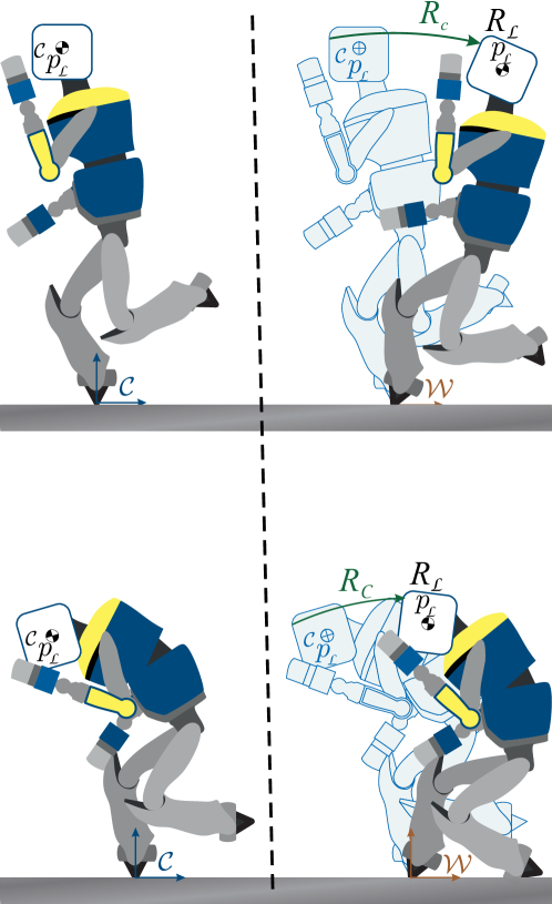
Figure 2: Two different configurations of the robot model, with fixed contact point, represented on the top and on the bottom. The IMU of each robot is represented with the circle in the head of the robot. For both top and bottom the left figure represents the position and orientation of the robot in the control frame $\mathcal{C}$ and the right one represents the same robot in the world frame with the unknown rotation $R_{\mathcal{C}}$. Note that the rotation $R_{\mathcal{C}}$ on the top and on the bottom is the same.

However such an ideal situation does not happen and there is a difference between the real position and orientation of the sensor in the world frame $p_{\mathcal{L}}\in\mathbb{R}^{3}$ and $R_{\mathcal{L}}\in SO(3)$ and their values in the control frame ${}^{\mathcal{C}}p_{\mathcal{L}}$ and ${}^{\mathcal{C}}R_{\mathcal{L}}$. This difference is usually a combination of translations and rotations, but in the absence of slipping, we can approximate the contact point position as being fixed. This means that the transformation between the control frame $\mathcal{C}$ and the world frame $\mathcal{W}$ is a 3D rotation $R_{\mathcal{C}}\in SO(3)$ around the origin, which means that $p_{\mathcal{L}}=R_{\mathcal{C}}\leavevmode\nobreak\ ^{\mathcal{C}}\!p_{\mathcal{L}}$ and $R_{\mathcal{L}}=R_{\mathcal{C}}\leavevmode\nobreak\ ^{\mathcal{C}}\!R_{\mathcal{L}}$ (see the right part of Figure 2).

With this model, let’s develop the expression of the desired signal of linear velocity $y_{v}$

$$y_{v} =R_{\mathcal{L}}^{T}\dot{p}_{\mathcal{L}}$$ (7)

$$=R_{\mathcal{L}}^{T}\;R_{\mathcal{C}}\;^{\mathcal{C}}\!\dot{p}_{\mathcal{L}}+R_{\mathcal{L}}^{T}\;R_{\mathcal{C}}\;S(\omega_{\mathcal{C}})\leavevmode\nobreak\ ^{\mathcal{C}}\!p_{\mathcal{L}}$$ (8)

$$=\leavevmode\nobreak\ ^{\mathcal{C}}\!R_{\mathcal{L}}^{T}\;{}^{\mathcal{C}}\!\dot{p}_{\mathcal{L}}+S(y_{g}-{}^{\mathcal{C}}\!\omega_{\mathcal{L}})\leavevmode\nobreak\ ^{\mathcal{C}}\!R_{\mathcal{L}}^{T}\;{}^{\mathcal{C}}\!p_{\mathcal{L}}$$ (9)

which is entirely reconstructable from available signals.

III-B The model with moving anchor point

The model of a fixed anchor can provide the required signals to build the attitude in the case of contact between one steady foot and the environment. However, a humanoid robot is required to perform bipedal walking, where the contact point transitions from one foot to the other, with a double support phase during the transition. One solution to this problem is to switch the contact position from one pivot point to the other during this double support phase. However, a discontinuous change in the pivot point generates a discontinuous $y_{v}$ signal which introduces artificial disturbances to the estimators. Therefore, a better solution is one where the transition is performed continuously. In that case we assume that we know the velocity $v_{a}$ of the anchor point $p_{a}$ in the world frame expressed in the control frame, i.e. such that $R_{\mathcal{C}}v_{a}=\dot{p}_{a}$. This velocity can be simply the derivative of the center of pressure reconstructed with the force sensor or any virtual point approximating this transition.

We attach the position of the control frame origin $p_{\mathcal{C}}$ at the position of the anchor point $p_{a}$ to keep the transformation as a pure 3D rotation around it. Note that varying this origin positions varies the values of variables expressed in the control frame, since they are translated by $p_{a}$. This model is sketched in Figure 1, where we show an example for a single and a double support. With this new frame definition, the position of the sensor in the world frame can be written as $p_{\mathcal{L}}=R_{\mathcal{C}}{}^{\mathcal{C}}p_{\mathcal{L}}+p_{\mathcal{C}}=R_{\mathcal{C}}{}^{\mathcal{C}}p_{\mathcal{L}}+p_{a}$.

Thanks to this expression we can develop the expression of the linear velocity $y_{v}$ as

$$y_{v} =R_{\mathcal{L}}^{T}\dot{p}_{\mathcal{L}}$$ (10)

$$=R_{\mathcal{L}}^{T}\;R_{\mathcal{C}}\;^{\mathcal{C}}\!\dot{p}_{\mathcal{L}}+R_{\mathcal{L}}^{T}\;R_{\mathcal{C}}\;S(\omega_{\mathcal{C}})\leavevmode\nobreak\ ^{\mathcal{C}}\!p_{\mathcal{L}}+R_{\mathcal{L}}^{T}\;R_{\mathcal{C}}\;v_{a}$$ (11)

$$=\leavevmode\nobreak\ ^{\mathcal{C}}\!R_{\mathcal{L}}^{T}\;{}^{\mathcal{C}}\!\dot{p}_{\mathcal{L}}+S(y_{g}-{}^{\mathcal{C}}\omega_{\mathcal{L}})\leavevmode\nobreak\ ^{\mathcal{C}}\!R_{\mathcal{L}}^{T}\leavevmode\nobreak\ {}^{\mathcal{C}}\!p_{\mathcal{L}}+{}^{\mathcal{C}}\!R_{\mathcal{L}}^{T}\;v_{a}$$ (12)

which is constructed algebraically from available signals.

Note that this formula may produce inconsistencies between the trajectory of the anchor point $p_{a}$ and its time derivative $v_{a}=R_{\mathcal{C}}^{T}\dot{p}_{a}$. This is because of the estimation error in the orientation of the control frame and the lack of yaw measurements, therefore we do not recommend using it for navigation. Nevertheless, what we need is only a good enough approximation of the real sensor velocity $v_{\mathcal{L}}$. We believe that the disturbance caused by this small modeling error has much less impact than the disturbance caused by the assumption of no linear acceleration made in classic approaches. Moreover, we show in the next section that this measurement is used through low-pass processing within a nonlinear complementary filter, to produce a reliable and theoretically grounded tilt estimation.

IV Tilt estimation

IV-A State and measurement definitions

Let’s define the following state variables

$$x_{1} \overset{\Delta}{=} v_{\mathcal{L}},$$ (13)

$$x_{2} \overset{\Delta}{=} R_{\mathcal{L}}^{T}e_{z},$$ (14)

with $x_{1}\in\mathbb{R}^{3}$ and $x_{2}\in\mathbb{S}^{2}$ , where the set $\mathbb{S}^{2}\subset\mathbb{R}^{3}$ is the unit sphere centered at the origin, and defined as

$$\mathbb{S}^{2}=\left\{x\in\mathbb{R}^{3}|\left\|x\right\|=1\right\}.$$

The variable $x_{1}$ is considered known using $y_{v}$, even if noisy. On the contrary, $x_{2}$ is the tilt we aim to estimate and cannot be obtained algebraically from the measurements.

From equations (5) and (13) we get

$$\dot{x}_{1}= -S(y_{g})x_{1}-g_{0}R_{\mathcal{L}}^{T}e_{z}+y_{a}.$$ (15)

This, together with the time-differentiation of $x_{2}$, provide us with the following state dynamic equations

$$\begin{cases}\dot{x}_{1}&=-S(y_{g})x_{1}-g_{0}x_{2}+y_{a},\\ \dot{x}_{2}&=-S(y_{g})x_{2}.\end{cases}$$ (16)

The system (16) is suitable for the observer synthesis presented hereinafter.

IV-B Two-stage observer designed in $\mathbb{R}^{3}\times\mathbb{R}^{3}\times\mathbb{S}^{2}$ and error dynamics

We define the observer for the state defined in Equations (13) and (14). It is designed in $\mathbb{R}^{3}\times\mathbb{R}^{3}\times\mathbb{S}^{2}$ and is given by

$$\begin{cases}\dot{\hat{x}}_{1}&=-S\left(y_{g}\right)\hat{x}_{1}-g_{0}\hat{x}^{\prime}_{2}+y_{a}+\alpha_{1}\left(y_{v}-\hat{x}_{1}\right)\\ \dot{\hat{x}}^{\prime}_{2}&=-S\left(y_{g}\right)\hat{x}^{\prime}_{2}-\frac{\alpha_{2}}{g_{0}}\left(y_{v}-\hat{x}_{1}\right)\\ \dot{\hat{x}}_{2}&=-S\left(y_{g}-\gamma S\left(\hat{x}_{2}\right)\hat{x}^{\prime}_{2}\right)\hat{x}_{2}\end{cases}$$ (17)

where $\alpha_{1}$, $\alpha_{2}$ and $\gamma$ are positive scalar gains, $\hat{x}_{1}$ and $\hat{x}_{2}$ are estimations of $x_{1}$ and $x_{2}$ respectively and $\hat{x}^{\prime}_{2}$ is an intermediate estimation of $x_{2}$.

Assuming perfect measurements and using the estimation errors defined as $\tilde{x}_{1}\overset{\Delta}{=}x_{1}-\hat{x}_{1}$, $\tilde{x}^{\prime}_{2}\overset{\Delta}{=}x_{2}-\hat{x}^{\prime}_{2}$ and $\tilde{x}_{2}=x_{2}-\hat{x}_{2}$, we get the error dynamics as

$$\begin{cases}\dot{\tilde{x}}_{1}&=-S(y_{g})\tilde{x}_{1}-\alpha_{1}\tilde{x}_{1}-g_{0}\tilde{x}^{\prime}{}_{2}\\ \dot{\tilde{x}}^{\prime}_{2}&=-S(y_{g})\tilde{x}^{\prime}_{2}+\frac{\alpha_{2}}{g_{0}}\tilde{x}_{1}\\ \dot{\tilde{x}}_{2}&=-S(y_{g})\tilde{x}_{2}+\gamma S^{2}(\hat{x}_{2})\tilde{x}_{2}-\gamma S^{2}(\hat{x}_{2})\tilde{x}^{\prime}_{2}\end{cases}$$ (18)

To run the analysis of errors, we set $z_{i}=R_{\mathcal{L}}\tilde{x}_{i}$ and $z^{\prime}_{2}=R_{\mathcal{L}}\tilde{x}^{\prime}{}_{2}$. Noticing $R_{\mathcal{L}}\hat{x}_{2}=e_{z}-z_{2}$, one gets

$$\begin{cases}\dot{z}_{1}&=-\alpha_{1}z_{1}-g_{0}z^{\prime}_{2}\\ \dot{z}^{\prime}_{2}&=\frac{\alpha_{2}}{g_{0}}z_{1}\\ \dot{z}_{2}&=\gamma S^{2}(e_{z}-z_{2})\left(z_{2}-z^{\prime}_{2}\right)\end{cases}$$ (19)

This new dynamics is autonomous and defines a time-invariant ordinary differential equation (ODE) which simplifies the stability analysis. Indeed, if one defines the error state $\xi\overset{\Delta}{=}\left(z_{1},z^{\prime}_{2},z_{2}\right)$ and the state space $\varUpsilon:=\mathbb{R}^{3}\times\mathbb{R}^{3}\times\mathbb{S}_{e_{z}}$ with $\mathbb{S}_{e_{z}}=\left\{z\in\mathbb{R}^{3}|\left(e_{z}-z\right)\in\mathbb{S}^{2}\right\}$, one can write (19) as $\dot{\xi}=F\left(\xi\right)$ where $F$ gathers the right-hand side of (19) and defines a smooth vector field on $\varUpsilon$.

Note that the first two lines of (17) constitute a separate tilt estimator defined in $\mathbb{R}^{3}\times\mathbb{R}^{3}$. A comparable tilt estimator can be found in [21]. We show hereinafter the convergence and the performances of this intermediate estimation. We show, afterward, that even if this intermediate estimator has very good performances, the estimator of (17) is an extension allowing to ensure that the tilt estimation respects the normality constraint and reject more disturbances.

IV-B1 Global exponential stability of the intermediate estimator

The two first lines of the observer given by equation (17) constitute an independent observer of the tilt which is designed in $\mathbb{R}^{3}\times\mathbb{R}^{3}$ where the vector $\hat{x}^{\prime}_{2}\in\mathbb{R}^{3}$ is the estimation of $x_{2}=R_{\mathcal{L}}^{T}e_{z}$. In this case the error dynamics is given by

$$\begin{cases}\dot{z}_{1}&=-\alpha_{1}z_{1}-g_{0}z^{\prime}_{2}\\ \dot{z}^{\prime}_{2}&=\frac{\alpha_{2}}{g_{0}}z_{1}\end{cases}$$ (20)

The dynamics is linear and autonomous. If one define the state $\xi^{\prime}:=\left(\nicefrac{{\alpha_{2}}}{{g_{0}}}z_{1},z^{\prime}_{2}\right)$ and the state space $\varUpsilon^{\prime}:=\mathbb{R}^{3}\times\mathbb{R}^{3}$, one can write (20) as $\dot{\xi}^{\prime}=A_{1}\xi^{\prime}$ where $A_{1}$ is constant and given by

$$A_{1}=\left[\begin{array}[]{ccc}-\alpha_{1}I_{3\times 3}&&-\alpha_{2}I_{3\times 3}\\ I_{3\times 3}&&0\end{array}\right]$$ (21)

This matrix allows us to state the following theorem.

Theorem 1

The system (20) is globally exponentially stable with respect to the origin $(0,0)$.

The proof comes from the stability of the matrix $A_{1}$.

The intermediate estimation $\hat{x}^{\prime}_{2}$ is not constrained to be normalized, despite $x_{2}=R_{\mathcal{L}}^{T}e_{z}$ being a unit vector. This constitutes a strength of this estimator, it will converge through the unit sphere from any initial value. This constitutes also two weaknesses. The first one is that a simple normalization of this estimation would risk undefined output and unbounded time-derivatives when the norm is close to zero. The second one is the sensitivity noise including the one which leads to the violation of normality constraint. The solution we propose is to add the third line of (17) to take profit from the convergence of $\hat{x}^{\prime}_{2}$ by tracking it while maintaining the normality constraint of the tilt estimation.

IV-B2 Almost global asymptotic stability of the full estimator

Let’s now consider the full estimator of Equation (17). We state the following theorem,

Theorem 2

The time-invariant ODE defined by (19) is almost globally stable with respect to the origin in the following sense: there exists an open dense set $\varUpsilon_{0}\subset\varUpsilon$ such that, for every initial condition $\xi_{0}\in\varUpsilon_{0}$, the corresponding trajectory converges asymptotically to ($0,0,0$).

The proof is presented in the appendix.

In addition to this asymptotic stability, we can also show good local performances around the desired equilibrium. It is indeed really important for humanoid robots to maintain precise tilt observation after the convergence of the estimation since it is involved in high gain closed-loop stabilization.

IV-B3 Local exponential stability

The good local performances of this estimator can be stated with the following theorem

Theorem 3

The time-invariant ODE defined by (19) provides local exponential convergence of the error $\xi$ to $\left(0,0,0\right)$.

The proof is presented in the appendix.

These theoretical guarantees are provided in the presence of precise measurements. But since the sensors are noisy and the velocity measurement has been produced with an approximation, we need to assess the performances and compare them with state-of-the-art approaches. Therefore in the next section, we present the implementation of this observer on a dynamical simulation and on the full-size humanoid robots HRP-5P and HRP-2KAI.

V Implementation

V-A Simulations

The approach validity can be assessed through a precise simulation. It is performed under the Matlab Simscape Multibody environment and uses a model of a simple 12 degrees of freedom biped robot weighing 42.6Kg with two rectangular feet. Figure 3 shows simulation screen captures. The contact with the environment is simulated with point contact at the four corners of each foot. With the effect of the weight, each contact point gets strictly inside the ground and generates a viscoelastic reaction force to simulate a compliant environment with stiffness of 10⁵ N/m and damping of 10³ $\nicefrac{{\text{N}s}}{{\text{m}}}$. These contact dynamics change the orientation of the contact when the forces change. The robot is set to rest configuration, with a little oscillation during convergence, and it is pushed twice, at 4 s and 14 s with 100 N and 300 N forces respectively, each lasting 0.1 s. The first one leads the robot to tilt and oscillate until convergence and the second makes the robot tip and fall. Note that this oscillation does not have a fixed point in the environment and therefore breaks assumptions of a fixed anchor point.

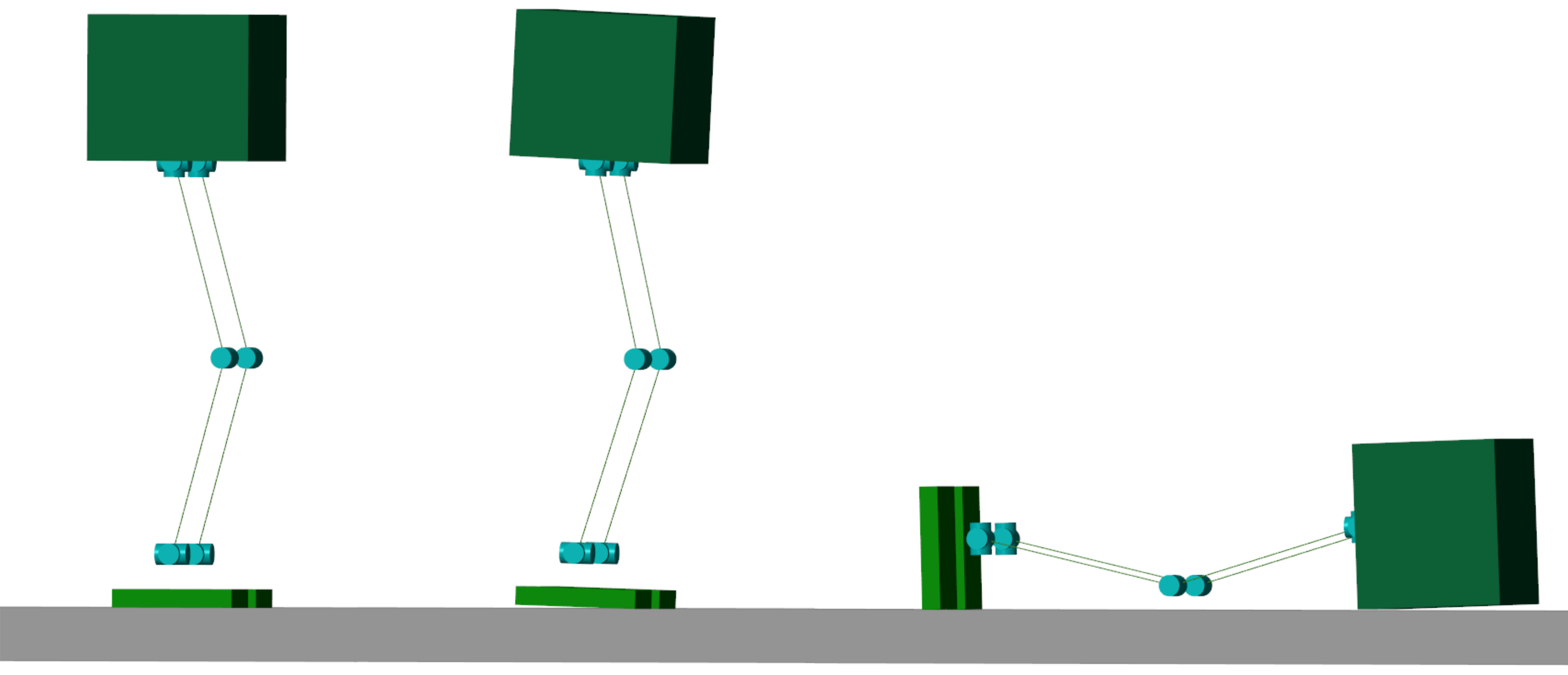
Figure 3: Screenshots of the simulation of the simple biped. The first image showing it in rest position, the second one after the small push and the third one after the big push.

The signals of an IMU consisting only of a gyrometer and an accelerometer were simulated with a uniform Gaussian noise with SD of 0.02 rad/s and 0.5 m/s² respectively. We use the position of the ZMP as a position of the anchor point. This allows us to generate the signal of the velocity $x_{1}$ using the method of Section III-B. Three state estimators were tested: (i) our estimator in $\mathbb{R}^{3}\times\mathbb{R}^{3}\times\mathbb{S}^{2}$ of Sec. IV-B, (ii) the estimator in $\mathbb{R}^{3}\times\mathbb{S}^{2}$ presented in our previous work [18], and the estimator of Hua 2016 from [19], which is also based on velocity-aided IMU and is comparable with our previous work, but with different dynamic properties. The parameters of the three estimators were $\alpha_{2}=k_{1}^{r}=20$, $\alpha_{1}=k_{1}^{v}=k_{2}^{v}=100$ and $\gamma=3$ and they were initialized to an error of 0.2 rad around the $X$ axis. The simulations are very slow (about 25 minutes) because of the variable time-step duration allowing for high precision in the simulation.

The plots of Figure 4 show the result of this simulation. The beginning includes the convergence phase of the estimators. We note that our estimator in $\mathbb{R}^{3}\times\mathbb{R}^{3}\times\mathbb{S}^{2}$ is the fastest to converge and the estimator of Hua 2016 is the slowest. The external forces are then applied at 4s where we can see (in the bottom) that the error has increased. This is only due to the modeling error arising from the assumption of an anchor point. However, by comparing the actual tilt with the estimation we can see that the tracking quality is good, especially the estimator in $\mathbb{R}^{3}\times\mathbb{R}^{3}\times\mathbb{S}^{2}$. Interestingly the estimator of Hua 2016 has good robustness to this modeling error compared to the estimator in $\mathbb{R}^{3}\times\mathbb{S}^{2}$. This could be specifically due to the slowness of Hua’s estimator providing it with stronger filtering of disturbances than our previous method. But the estimation of our method in $\mathbb{R}^{3}\times\mathbb{R}^{3}\times\mathbb{S}^{2}$ is still better. However, the most interesting part is the fall induced at 14s where all estimators have rather good tracking thanks to their convergence properties. Nevertheless, If we focus on the error on the bottom, we can see that the previous estimators have an increased error while our estimator did not suffer a lot from this important disturbance. It is interesting to observe also, in the estimation on the Y axis, the noise sensitivity of the methods. We can see that our method in $\mathbb{R}^{3}\times\mathbb{R}^{3}\times\mathbb{S}^{2}$ has the best filtering, followed by Hua 2016 and then our previous method in $\mathbb{R}^{3}\times\mathbb{S}^{2}$.

These results confirm the good behavior of the estimator in $\mathbb{R}^{3}\times\mathbb{R}^{3}\times\mathbb{S}^{2}$ which is the fastest to converge without being too sensitive to noises and disturbances.

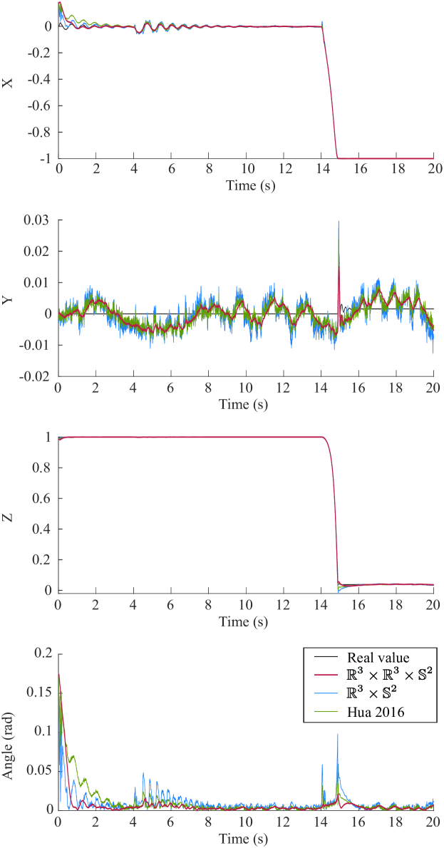
Figure 4: Plot showing the evolution of estimations from three tilt observers for the simulated biped. The top three figures show each component of the tilt estimation $\hat{x}_{2}$ compared to the real value. The bottom shows the error angle for the three estimators.

V-B Open-source implementation on HRP-5P and HRP-2KAI

The estimator in $\mathbb{R}^{3}\times\mathbb{R}^{3}\times\mathbb{S}^{2}$, coupled with the linear velocity reconstruction exposed in the previous section has been implemented in the control framework of two robots, HRP-5P [22] and HRP-2KAI [23]. Both are full-scale humanoid robots of 182 cm, 101 kg and 170cm, 65Kg respectively, and are equipped with 37 and 32 degrees of freedom, developed at the National Institute of Advanced Industrial Science and Technology (AIST). Both robots are controlled in a real-time framework based on Open-RTM middleware developed in AIST as well. Nevertheless, the implementation of the tilt estimator has rather been performed as a standalone state observation open-source C++ library [24], called simply tilt estimator.

The tilt estimation is used in the real-time balance control of the robots described in [25], which requires an estimation of the position and the velocity of the center of mass. To do that, let us assume that the positions of the feet are known. They can be for example provided by a footstep planner. Note that although a precise location is required for the navigation, it is not necessary for the balance control. From the feet position, the control frame $\mathcal{C}$ is built. The anchor $p_{a}$, at the origin of $\mathcal{C}$, can be described by a weighted ratio of the feet locations, the weights being the desired vertical forces at each foot. This definition allows us to keep a continuous trajectory of the origin while successfully transiting from one foot to another, and to know the velocity of this origin $v_{a}$. The position ${}^{\mathcal{C}}p_{\mathcal{L}}$ and orientation ${}^{\mathcal{C}}R_{\mathcal{L}}$ of the IMU in $\mathcal{C}$ are known from the model and the encoders, and the linear and angular velocities ${}^{\mathcal{C}}\dot{p}_{\mathcal{L}}$ and ${}^{\mathcal{C}}\omega_{\mathcal{L}}$ can be estimated by using finite differences. This allows implementing the estimator as described in Section III-B. The desired yaw coming from the bipedal locomotion planner is combined with the estimated tilt using the TRIAD method [26], where we construct a virtual magnetometer by using the desired yaw angle without disturbing the estimation of the tilt. This attitude estimation provides us with the orientation of the floating-base, for instance, the waist, and the position of the anchor point gives us the floating-base position. The angular and linear velocities of the base are obtained with the gyrometer and the anchor point. Having estimated the state of the floating-base it is straightforward to estimate the state of the center of mass. This is the necessary feedback that is required to implement the balance control.

The balance control is realized by a PID controller of the error between the desired and the estimated Divergent Component of Motion (DCM). The DCM is calculated as $\xi=c+\frac{1}{\rho_{c}}\dot{c}$, where $c$ and $\dot{c}$ are the CoM position and its velocity, and $\rho_{c}$ is the natural frequency of the dynamics of the equivalent inverted pendulum [27]. The DCM-based controller modifies the reference center of pressure, from which the reference forces and moments of the feet are computed. Then, a damping control, described in [2], modifies the relative position of the feet and their orientation to realize the foot reference force and moment. Finally, the joint angles are calculated by using the prioritized inverse kinematics scheme proposed by [28] and sent to the joint servos. Figure 5 illustrates the previous description.

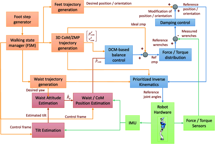
Figure 5: A simplified diagram of the bipedal locomotion control framework. Elements in red are components related to the estimation. Elements in yellow are components used to generate desired values. Elements in blue are components related to the control. Elements in green belong to the robot.

Since there is no ground truth value for the real robot orientation, we test the performance of the estimator by assessing the stability in two experiments. The first one consists of leaning the chest forward by 25 degrees and coming back to the vertical, all in 2 seconds. This allows us to check the reactivity of the estimator to fast tilt changes, similarly to what happens in the falling simulation above. The second test is walk forward, this will assess the behavior concerning impacts and modifications of the contact point. All these experiments were successful and the balance of both robots could be maintained. Screen captures of these tests are available in Figure 6. For the case of HRP-5P, we show, in Figure (7), the measurements of the IMU together with the tilt estimation during each experiment. There we can see the tracking of the inclination of the chest and the quality of estimation during walking. We can evaluate the gait impacts by looking at the accelerometer measurements.

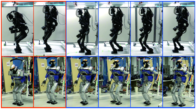
Figure 6: Screen capture of the robots (HRP-5P on top and HRP-2KAI on the bottom) performing the test motions. The two leftmost images show the leaning task and the remaining images show the walking motion.

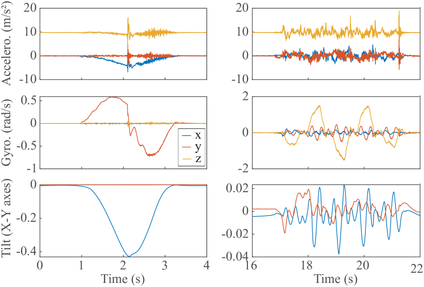
Figure 7: Plots showing the chest leaning test on the left and the walking test on the right. The accelerometer measurements are on the top, the gyrometer measurements on the middle, and the tilt estimation on the bottom. The Z axis has been removed from the tilt estimation for legibility and can be reconstructed knowing that it is the positive solution to the vector normality constraint.

VI Conclusion

We have presented a Lyapunov stable tilt estimator that can be applied to humanoid robots. We have shown how the presence of an anchor position, even if it is moving, can be exploited to algebraically produce approximations of the linear velocity of the sensor. This new signal allows us to use estimators dedicated to velocity-aided IMUs. We have shown the theoretical guarantees of almost global asymptotic stability and local exponential convergence of the presented two-stage estimator. Finally, we have studied the performance of the estimator on a dynamic simulator of a simple biped and have shown the stability of real robots when used within a closed-loop balance control framework.

Appendix A Proofs

A-A Proof of theorem 2

Proof:

We define the positive-definite differentiable function $V:\varUpsilon\rightarrow\mathbb{R}^{+}$ radially unbounded over $\varUpsilon$

$$V \overset{\Delta}{=}\frac{\alpha_{2}}{8\alpha_{1}g_{0}}\left\|z_{1}\right\|{}^{2}+\frac{1}{8\alpha_{1}g_{0}}\left\|\alpha_{1}z_{1}+g_{0}z^{\prime}_{2}\right\|{}^{2}$$

$$\qquad+\frac{\alpha_{1}g_{0}}{4\alpha_{2}}\left\|z^{\prime}_{2}\right\|{}^{2}+\frac{1}{2\gamma}\left\|z_{2}\right\|{}^{2}.$$ (22)

Using the error dynamics given by (18), the time derivative of $V$ is then given by

$$\dot{V} =-\frac{\alpha_{1}^{2}}{4g_{0}}z_{1}^{T}z_{1}-\frac{g_{0}}{4}z_{2}^{\prime T}z{}_{2}^{\prime}+\frac{1}{\gamma}z_{2}^{T}\dot{z}_{2},$$ (23)

$$\dot{V} =-\frac{\alpha_{1}^{2}}{4g_{0}}z_{1}^{T}z_{1}-\frac{g_{0}}{4}z{}_{2}^{\prime T}z{}_{2}^{\prime}+z_{2}^{T}S^{2}(e_{z})z_{2}$$

$$\qquad-z_{2}^{T}S(e_{z})S(e_{z}-z_{2})z^{\prime}_{2}$$ (24)

If we define the new vector $w=S(e_{z})z_{2}$, we can write

$$\dot{V}=-\frac{\alpha_{1}^{2}}{4g_{0}}z_{1}^{T}z_{1}-\frac{g_{0}}{4}z_{2}^{\prime T}z{}_{2}^{\prime}-w^{T}w+w^{T}S(e_{z}-z_{2})z^{\prime}_{2}$$

and then

$$\dot{V}\leq-\frac{\alpha_{1}^{2}}{4g_{0}}\left\|z_{1}\right\|^{2}-\frac{g_{0}}{4}\left\|z^{\prime}_{2}\right\|^{2}-\left\|w\right\|^{2}+\left\|w\right\|\left\|z^{\prime}_{2}\right\|$$

We define the vector $\varrho=[\begin{array}[]{ccc}\left\|z_{1}\right\|&\left\|z^{\prime}_{2}\right\|&\left\|w\right\|\end{array}]^{T}$, giving

$$\dot{V}\leq-\varrho^{T}H\varrho$$

where $H=\left[\begin{array}[]{ccccc}\frac{\alpha_{1}^{2}}{4g_{0}}&0&0\\ 0&\frac{g_{0}}{4}&-\frac{1}{2}\\ 0&-\frac{1}{2}&1\end{array}\right]$, a positive definite matrix. It means that $\dot{V}\leq 0$ and more specifically $\dot{V}<0$ if $(z_{1},z^{\prime}{}_{2},z_{2})$ is not an equilibrium point.

The linearized system around the equilibrium $(0,0,2e_{z})$ is given by the following dynamics

$$\dot{X}=A_{2}X,$$ (25)

with $X=\left[\begin{array}[]{ccc}\left(z_{1}\right)^{T}&\left(z^{\prime}_{2}\right)^{T}&\left(z_{2}-2e_{z}\right)^{T}\end{array}\right]^{T}$ and $A_{2}$ being a constant matrix having the form

$$A_{2}=\left[\begin{array}[]{ccc}-\alpha_{1}I_{3\times 3}&-g_{0}I_{3\times 3}&0\\ \frac{\alpha_{2}}{g_{0}}I_{3\times 3}&0&0\\ 0&-\gamma S^{2}(e_{z})&-\gamma S^{2}(e_{z})\end{array}\right]$$ (26)

where $I_{3\times 3}$ is the $3\times 3$ identity matrix. The characteristic polynomial of the matrix $A_{2}$ is given by

$$P(\lambda)=\left(\lambda^{2}+\alpha_{1}\lambda+\alpha_{2}\right)^{3}\lambda\left(\lambda-\gamma\right)^{2}.$$ (27)

This polynomial has the following double real positive root

$$\lambda=\gamma>0,$$ (28)

It can be verified that the linearized system at $(0,0,2e_{z})$ admits positive real eigenvalues. Hence the origin is almost globally asymptotically stable.

This completes the proof of the theorem. ∎

A-B Proof of Theorem 3

Proof:

The estimator has a unique stable equilibrium point defined by $\xi=\left(0,0,0\right)^{T}$. The linearization of the error dynamics of (19) around this point is defined in the tangent space to the state space $\varUpsilon$, which happens to be $T\left(\varUpsilon\right)=\mathbb{R}^{3}\times\mathbb{R}^{3}\times\mathbb{R}^{2}$. We define the state $\xi_{p}\overset{\Delta}{=}\left(z_{1},z^{\prime}_{2},z_{2p}\right)$ where $z_{2p}\in\mathbb{R}^{2}$ is the orthogonal projection of $z_{2}$ on the horizontal plane. The linearized dynamics is given by $\dot{\xi}_{p}=A_{3}\xi_{p}$ with $A_{3}$ being a constant matrix having the form

$$A_{3}=\left[\begin{array}[]{ccccc}-\alpha_{1}I_{3\times 3}&&-g_{0}I_{3\times 3}&&0\\ \frac{\alpha_{2}}{g_{0}}I_{3\times 3}&&0&&0\\ 0&&I_{2\times 3}&&-\gamma I_{2\times 2}\end{array}\right]$$ (29)

where $I_{2\times 3}=\left[\begin{array}[]{ccc}1&0&0\\ 0&1&0\end{array}\right]$. The matrix $A_{3}$ is Hurwitz giving the stability of the linearized dynamics. QED. ∎

References

- [1] P.-B. Wieber, R. Tedrake, and S. Kuindersma. Modeling and Control of Legged Robots, pages 1203–1234. Springer International Publishing, Cham, 2016.
- [2] S. Kajita, M. Morisawa, K. Miura, S. Nakaoka, K. Harada, K. Kaneko, F. Kanehiro, and K. Yokoi. Biped walking stabilization based on linear inverted pendulum tracking. In IEEE/RSJ International Conference on Intelligent Robots and Systems (IROS), 2010.
- [3] P. Allgeuer and S. Behnke. Robust sensor fusion for robot attitude estimation. In 2014 IEEE-RAS International Conference on Humanoid Robots, pages 218–224. IEEE, 2014.
- [4] X. Mao, X. Wen, Y. Song, W. Li, and G. Chen. Eliminating drift of the head gesture reference to enhance google glass-based control of an nao humanoid robot. International Journal of Advanced Robotic Systems, 14(2):1729881417692583, 2017.
- [5] Michael Bloesch, Marco Hutter, Mark Hoepflinger, Stefan Leutenegger, Christian Gehring, C David Remy, and Roland Siegwart. State Estimation for Legged Robots - Consistent Fusion of Leg Kinematics and {IMU}. In Proceedings of Robotics: Science and Systems, Sydney, Australia, jul 2012.
- [6] N. Rotella, M. Bloesch, L. Righetti, and S. Schaal. State Estimation for a Humanoid Robot. In IEEE/RSJ Intenational Conference on Intelligent Robots and Systems (IROS), 2014.
- [7] J. Eljaik, N. Kuppuswamy, and F. Nori. Multimodal sensor fusion for foot state estimation in bipedal robots using the extended Kalman filter. In 2015 IEEE/RSJ International Conference on Intelligent Robots and Systems (IROS), pages 2698–2704, Sep. 2015.
- [8] Mehdi Benallegue and Florent Lamiraux. Humanoid flexibility deformation can be efficiently estimated using only inertial measurement units and contact information. In 2014 IEEE-RAS International Conference on Humanoid Robots, pages 246–251, 2014.
- [9] Pierre Latteur, Sébastien Goessens, Jean-Sébastien Breton, Justin Leplat, Zhao Ma, and Caitlin Mueller. Drone-Based Additive Manufacturing of Architectural Structures. 2015.
- [10] Paweł Wawrzyński, Jakub Możaryn, and Jan Klimaszewski. Robust estimation of walking robots velocity and tilt using proprioceptive sensors data fusion. Robotics and Autonomous Systems, 66:44 – 54, 2015.
- [11] M. Vigne, A. El Khoury, M. Masselin, F. Di Meglio, and N. Petit. Estimation of multiple flexibilities of an articulated system using inertial measurements. In 2018 IEEE Conference on Decision and Control (CDC), pages 6779–6785. IEEE, 2018.
- [12] S. Nobili, M. Camurri, V. Barasuol, M. Focchi, D. Caldwell, C. Semini, and M. Fallon. Heterogeneous sensor fusion for accurate state estimation of dynamic legged robots. In Proceedings of Robotics: Science and Systems, Cambridge, Massachusetts, July 2017.
- [13] Maurice F Fallon, Matthew Antone, Nicholas Roy, and Seth Teller. Drift-free humanoid state estimation fusing kinematic, inertial and lidar sensing. In 2014 IEEE-RAS International Conference on Humanoid Robots, pages 112–119. IEEE, 2014.
- [14] R. Kuindersma, S.and Deits, M. Fallon, A. Valenzuela, H. Dai, F. Permenter, T. Koolen, P. Marion, and R. Tedrake. Optimization-based locomotion planning, estimation, and control design for the atlas humanoid robot. Autonomous robots, 40(3):429–455, 2016.
- [15] Ross Hartley, Maani Ghaffari, Ryan M Eustice, and Jessy W Grizzle. Contact-aided invariant extended kalman filtering for robot state estimation. The International Journal of Robotics Research, 39(4):402–430, 2020.
- [16] R. Hartley, M. Ghaffari Jadidi, J. Grizzle, and R. M Eustice. Contact-aided invariant extended kalman filtering for legged robot state estimation. In Proceedings of Robotics: Science and Systems, Pittsburgh, Pennsylvania, June 2018.
- [17] Axel Barrau and Silvère Bonnabel. The invariant extended kalman filter as a stable observer. IEEE Transactions on Automatic Control, 62(4):1797–1812, 2016.
- [18] M. Benallegue, A. Benallegue, and Y. Chitour. Tilt estimator for 3D non-rigid pendulum based on a tri-axial accelerometer and gyrometer. In 2017 IEEE-RAS 17th International Conference on Humanoid Robotics (Humanoids), pages 830–835. IEEE, nov 2017.
- [19] M.-D. Hua, P. Martin, and T. Hamel. Stability analysis of velocity-aided attitude observers for accelerated vehicles. Automatica, 63:11–15, jan 2016.
- [20] M. Benallegue, A. Benallegue, R. Cisneros, and Y. Chitour. Velocity-aided IMU-based Attitude Estimation. "https://hal.archives-ouvertes.fr/hal-02485372", 2020.
- [21] P. Martin, I. Sarras, M.-D. Hua, and T. Hamel. A global exponential observer for velocity-aided attitude estimation. arXiv preprint arXiv:1608.07450, aug 2016.
- [22] K. Kaneko, H. Kaminaga, T. Sakaguchi, S. Kajita, M. Morisawa, I. Kumagai, and F. Kanehiro. Humanoid robot HRP-5P: An electrically actuated humanoid robot with high-power and wide-range joints. IEEE Robotics and Automation Letters, 4(2):1431–1438, 2019.
- [23] K. Kaneko, M. Morisawa, S. Kajita, S. Nakaoka, T. Sakaguchi, R. Cisneros, and F. Kanehiro. Humanoid robot HRP-2Kai - improvement of HRP-2 towards disaster response tasks. In 2015 IEEE-RAS 15th International Conference on Humanoid Robots (Humanoids), pages 132–139. IEEE, 2015.
- [24] State-estimator - open-source c++ library source code, 2019. "https://github.com/mehdi-benallegue/state-observation".
- [25] M. Morisawa, N. Kita, S. Nakaoka, K. Kaneko, S. Kajita, and F. Kanehiro. Biped locomotion control for uneven terrain with narrow support region. In 2014 IEEE/SICE International Symposium on System Integration, pages 34–39. IEEE, 2014.
- [26] M. D. Shuster and S D. Oh. Three-axis attitude determination from vector observations. Journal of guidance and Control, 4(1):70–77, 1981.
- [27] J. Englsberger, C. Ott, and A. Albu-Schäffer. Three-dimensional bipedal walking control using divergent component of motion. In 2013 IEEE/RSJ International Conference on Intelligent Robots and Systems, pages 2600–2607. IEEE, 2013.
- [28] O. Kanoun, F. Lamiraux, and P.-B. Wieber. Kinematic control of redundant manipulators: Generalizing the task-priority framework to inequality task. IEEE Transactions on Robotics, 27(4):785–792, 2011.