Dropping Standardized Testing for Admissions Trades Off Information and Access

Abstract

We study the role of information and access in capacity-constrained selection problems with fairness concerns. We develop a theoretical statistical discrimination framework, where each applicant has multiple features and is potentially strategic. The model formalizes the trade-off between the (potentially positive) informational role of a feature and its (negative) exclusionary nature when members of different social groups have unequal access to this feature.

Our framework finds a natural application to recent policy debates on dropping standardized testing in college admissions. Our primary takeaway is that the decision to drop a feature (such as test scores) cannot be made without the joint context of the information provided by other features and how the requirement affects the applicant pool composition. Dropping a feature may exacerbate disparities by decreasing the amount of information available for each applicant, especially those from non-traditional backgrounds. However, in the presence of access barriers to a feature, the interaction between the informational environment and the effect of access barriers on the applicant pool size becomes highly complex. In this case, we provide a threshold characterization regarding when removing a feature improves both academic merit and diversity. Finally, using calibrated simulations in both the strategic and non-strategic settings, we demonstrate the presence of practical instances where the decision to eliminate standardized testing improves or worsens all metrics.

1 Introduction

Recent debates on the use of standardized testing in college admissions have increasingly garnered national attention, initially during the COVID-19 pandemic as test centers shut down and schools were forced to reconsider their admissions practices (Anderson, 2020). Independently of the COVID-19 pandemic, in an attempt to increase equity and diversity in admissions, the University of California (UC) settled a lawsuit by eliminating all consideration of SAT and ACT scores for admissions and scholarships through 2025, following an earlier decision to suspend testing requirements and ultimately design its own test (Nieto del Rio, 2021). Most recently, in response to the United States Supreme Court ruling to end race-based affirmative action, more colleges are expected to drop those requirements permanently, “responding to critics who say the tests favor students from wealthier families” and at the same time, protecting schools from lawsuits (Saul, 2023).

These discussions primarily center on highly selective institutions and their efforts to shape the student body through the admissions process. These schools promise great opportunities to their students, but – due to perceived capacity constraints – limit their acceptances to students that they deem to have high potential in academics, athletics, creative endeavors, or leadership and service (Espenshade and Radford, 2013). They typically attempt to identify these students through a combination of standardized tests, high school grades, letters of recommendation, personal essays, and extracurricular activities (Espenshade and Radford, 2013; Zwick, 2002).

The question is whether each of these components, and the application as a whole, allows the schools to assess individuals from different backgrounds effectively and ‘fairly,’ including students from different racial, ethnic, and socioeconomic groups. Implicitly, the debate concerns how to design an admission policy to aid fair and efficient decision-making, in terms of both deciding which information to collect from applicants and how to use this information. Our exposition focuses on the context of college admissions; however, our model and the questions we ask are more broadly applicable to other settings of information design and fair decision-making in capacity-constrained settings, such as labor markets, award committees, and social welfare programs. In each of these cases, the decisions are being made on limited information but have far-reaching consequences for employment or education opportunities. Thus, it is important to analyze these policies and their potential disparate impact across different groups of applicants.

Background. A high-profile debate has surrounded the use of standardized testing for admissions, in which social scientists and education experts have highlighted specific fairness concerns. Test critics argue that tests exhibit racial gaps (Reardon, 2011) and reinforce inequality in higher education (Reeves and Halikias, 2017). Espenshade and Radford (2013) find that only 8% of lower-income compared to 78% of high-income students use a test preparation service. The testing process is expensive and time-consuming; Hyman (2016) finds that “for every ten poor students who score college-ready on the ACT or SAT, there are an additional five poor students who would score college-ready but who take neither exam” and so cannot apply to colleges that require it.

Supporters of testing argue that it is “a systematic means of collecting information,” thereby contributing to decision-making when used appropriately (Phelps, 2005). Some supporters claim that tests actually help schools evaluate under-represented minorities; in the absence of standardized testing, “a capable student from a little-known school in the South Bronx may be more challenging to evaluate,” further benefiting students from privileged – and historically familiar – backgrounds (Bellafante, 2020). A report released by University of California explicitly uses the language of precision and predictive power of test scores compared to other features: “The predictive power of the standardized test scores is higher for those student groups who are under-represented […] Thus, consideration of test scores allows campuses to select those students from under-represented groups who are more likely to earn higher grades and to graduate on time […] One implication is that consideration of test scores allows greater precision when selecting from [under-represented minority] populations” (University of California Standardized Testing Task Force, 2020). MIT in 2022 reinstated the SAT, highlighting that their “research shows standardized tests help us better assess the academic preparedness of all applicants, and also help us identify socioeconomically disadvantaged students who lack access to advanced coursework or other enrichment opportunities that would otherwise demonstrate their readiness” (Schmill, 2022). Other application components such as recommendation letters (Dutt et al., 2016) and application essays (Alvero et al., 2021) may also be unreliable. A school that does not consider test scores must rely more heavily on these components.

Research questions. The competing claims from critics and supporters largely center around two issues: access and information. We develop a model to capture these arguments in favor of and against dropping test scores and formalize the underlying trade-off. The model considers a Bayesian school that wishes to admit students based on their skill level, which we refer to as “academic merit,” and also values the “diversity” of the admitted class. Not every student applies to a school that requires testing – they may face group-dependent barriers or costs to applying. The school admits applicants to meet a capacity constraint and tries to maximize the average academic merit of the accepted cohort. However, it has imperfect knowledge of the students skills and instead must rely on noisy and potentially biased signals, one of which is the test score. The school decides whether to require the test score; the decision affects both who applies and how the school evaluates applicants.

We then provide a framework for evaluating potential trade-offs in these decisions. In particular, alongside the academic merit objective, we analyze two fairness notions: diversity and individual fairness. The former captures group-level disparities. The latter quantifies disparities in individual opportunities, by measuring the difference in the admissions probability between two individuals of equal skill but different demographic groups. We focus on the trade-off between two effects:

Differential informativeness.

Colleges often have better information – through, e.g., familiar letter writers and transcripts – on students from privileged backgrounds, and so can better estimate their true academic merit. Standardized testing reduces this measurement gap, and so in particular helps colleges identify well-qualified, non-traditional students.

Applicant pool composition due to disparate access and strategic behavior

Some students – especially those from disadvantaged backgrounds – either do not take standardized tests or do not report their scores, due to cost and other exogenous access barriers. Without a test score, students cannot apply to a school with a test requirement, even if they are well-qualified. Dropping the requirement thus expands the applicant pool but also alters its composition at different rates across groups.

We further study when applicant composition is a result of strategic decisions made by students, who can choose whether to pay testing and application costs, making the decision as a function of their other features.

Contributions and overview. Given these effects, we study: Under what settings of informativeness and disparate access should standardized testing be dropped from admissions, if a college values both diversity and academic merit? Furthermore, what is the effect on these metrics when students can overcome disparate application costs, i.e., when students are strategic? To the best of our knowledge, our paper is the first theoretical study examining the impact of eliminating testing requirements in college admissions.

Modeling-wise, we introduce a Bayesian model that extends the classic statistical discrimination theory by Phelps (1972) to include multiple application components, access assymetries to some feature and potentially strategic student behavior and multiple schools (see Section 1.1 for a more detailed comparison). Our multi-feature model allows us to study the design of the information structure used in a selection process, and provide a testable framework for reasoning about how the new feature would interact with the current set of features, including when applicants can make strategic decisions. More broadly, we thus believe that our work provides a useful conceptual framework of independent interest, for studying emerging problems in fair decision-making and public policy.

From a technical insights perspective, we formalize a trade-off between informativeness and access, two basic arguments in favor of and against the inclusion of a given feature, and show how the set of features required influences the admitted class’s academic merit and diversity, through these competing effects. Our main technical insight shows that differences in the total variance of features lead to information disparities across groups: even though the school manages to correct for the existing mean bias in the features of different groups, it is generally impossible to correct for variance – this variance effect is thus central when considering the set of features to use. We characterize the settings where dropping test scores introduces a trade-off between diversity and academic merit and where it simultaneously improves or worsens all objectives.

We further extend the model to consider the effect of students’ strategic test-taking behavior and two schools simultaneously admitting students. Students can choose to pay (potentially heterogeneous) costs to take the test and apply to a school that requires it. At equilibrium, students self-select to apply to a test-based school if their perceived probability of admission outweights their relative cost-to-valuation ratio. We find that such strategic behavior disproportionately affects applicant pool composition but not always at the expense of the group facing higher test costs. Additionally, in the case with two schools, where only the top school requires the test, we uncover an interesting discontinuity in the students’ self-selecting behavior, which in turn leads to a potential mismatch between academic merit and the ranking of the school.

Finally, we use our model to perform calibrated simulations based on real applicant data from the University of Texas at Austin. Our results establish that there exist practical settings both in which dropping testing concurrently worsens or improves all metrics, and that such effects especially depend on the strategic behavior of potential applicants. Thus, our primary takeaway for practice is that the decision to drop testing cannot be made without jointly considering the interaction between the information provided by other features relative to test scores and how dropping the test requirement affects the applicant pool composition. This interaction between information and access is complex.

Organization. Section 1.1 discusses the related literature. Section 2 introduces our baseline model. Section 3 provides intuition on the effect of informativeness and test access in our model. In Section 4, we formalize a trade-off between informativeness and access when students may face access barriers to taking the test. In Section 5, we extend the model to include students’ strategic test-taking behavior and two schools. Finally, in Section 6, we present calibrated simulations based on UT Austin data.

1.1 Related Work

Our work broadly relates to the study of discrimination and admissions in the economics and fair machine learning and operations communities.

Economics of discrimination. In economics, there are two lines of related work: discrimination theories (Becker, 1957), especially statistical discrimination (Phelps, 1972; Arrow, 1971) as well as theoretical models of affirmative action in student admissions (e.g., Chade et al. (2014); Fu (2006); Abdulkadiroğlu (2005); Chan and Eyster (2003); Kamada and Kojima (2019); Epple et al. (2006); Avery et al. (2006); Fershtman and Pavan (2020)). There is also an important line of empirical work investigating the implications of affirmative action (e.g., Arcidiacono et al. (2011); Bagde et al. (2016); Backes (2012); Bleemer (2020)) and race-neutral alternatives such as top percent plans and holistic reviews (e.g., Bleemer (2023); Kapor (2020); Ellison and Pathak (2021); Long (2004); Bleemer (2018)).

From a conceptual viewpoint, our work is most closely related to the statistical discrimination theory of Phelps (1972), which – surprisingly – is rarely adopted in the admissions literature (except Emelianov et al. (2020); Kannan et al. (2019)). Emelianov et al. (2020) use Phelps’ model to study how differential variance of a single feature affects the admissions decisions of a school that greedily admits students with the highest test scores, without factoring in the differential variance.

Both our work and Emelianov et al. (2020) adopt the seminal theory of statistical discrimination (Phelps, 1972). However, our work moves beyond Emelianov et al. (2020) and Phelps (1972), as well as the standard matching-based approach of other theoretical models (e.g., Chade et al. (2014); Abdulkadiroğlu (2005); Karni et al. (2021)), in several ways. To the best of our knowledge, our paper is the first to extend Phelps’ model to multiple features with non-identical distributions and access asymmetries to some feature. We further combine such statistical discrimination with a model of strategic student behavior. These modeling contributions allow us to study the complex interactions between the test and several other factors, including the remaining application components, access barriers and test costs (that induce student strategic behavior). Furthermore, our multi-feature model allows the decision-maker to potentially remove a feature, thus enabling us to reason about policy changes such as dropping standardized testing in a tractable manner. On the other hand, Emelianov et al. (2020) include an effort component in their model, which we do not consider. In their framework, candidates have the ability to increase the mean of their single feature at a quadratic cost. Their finding that affirmative action can enhance both diversity and academic merit arises from the balancing of average efforts across groups in certain equilibria.

Fairness in machine learning and operations. Recent machine learning work applies fairness notions to admissions and related allocation problems, studying implicit bias (Kleinberg and Raghavan, 2018; Emelianov et al., 2020; Faenza et al., 2020), downstream effects (Kannan et al., 2019), grade signaling (Immorlica et al., 2019), greenling (Borgs et al., 2019), school choice (Allman et al., 2022), bus scheduling (Banerjee and Smilowitz, 2019), and classification algorithms (Liu et al., 2020; Hu et al., 2019). More broadly, our work contributes to the emerging literature on fairness in operational contexts (e.g., Bertsimas et al. (2011); Manshadi et al. (2021); Baek and Farias (2021); Monachou and Ashlagi (2019); Sinclair et al. (2022); Cohen et al. (2022); Kallus and Zhou (2021)), especially with respect to equity in education (Smilowitz and Keppler, 2020).

A line of literature specializes on different types of barriers for students, including implicit bias (Faenza et al., 2020) and when only one group can take the test multiple times (Niu et al., 2022). These barriers affect the treatment of applicants, but do not prevent students from even applying, as is our focus in our baseline model. In relation to our strategic setting, note that Faenza et al. (2020) do not consider strategic students. Niu et al. (2022) allow students to decide whether to take the test twice or not but their model does not include costs and students have only binary skill levels.

Finally, an extended abstract of a preliminary version of our results appears in Garg et al. (2021). A follow-up paper (Liu and Garg, 2021) extends our model to provide (im)possibility results under test-optional policies (see also Dessein et al. (2023)). Castera et al. (2022) also build upon our work to study disparities due to differential correlation in a two-college setting (although they depart from the standard notion of statistical discrimination that we use here, in the sense that each college uses the same ranking distribution for both groups). Recently, using data from the Education Longitudinal Study of 2002, Borghesan (2022) finds that banning the SAT leads to a small increase in the population of low-income students but has a negligible effect on under-represented minority students.

2 Model

We develop a model where the school can design their admissions procedure and, in particular, choose the information that it requires the applicants to submit.

We consider a continuum of students and a single school. A unit mass of students is applying to college. Each student belongs to a group $g\in\{A,B\}$, and the mass of students in group $B$ is $\pi$. Each student has a latent (unobserved) skill level $q$, Normally distributed according to $\mathcal{N}(\mu,\sigma^{2})$ identically for each group, as well as a set of observed features $\operatorname{\bm{\theta}}=(\theta_{1},\ldots,\theta_{K})$. Each $\theta_{k}$ is a noisy function of $q$, i.e., $\theta_{k}=q+\epsilon_{k}$, $k=1,\ldots,n$, with Gaussian noise $\epsilon_{k}~{}\sim~{}N(\mu_{gk},\sigma_{gk}^{2})$. The distribution of noise $\epsilon_{k}$ is feature- and group-dependent, but each $\epsilon_{k}$ is drawn independently across features and students. Features represent application components like recommendation letters, grades, and test scores.

Students differ in their access to the features. When a student does not have access to feature $K$, then they cannot apply to a school that requires it. In our primary model, only a fraction $\gamma_{g}$ of group $g\in\{A,B\}$ has access to the full set of features $\operatorname{\textsc{full}}=\{1,\dots,K\}$, i.e., $\operatorname{\bm{\theta}}=(\theta_{1},\dots,\theta_{K})$; the remainder only has access to the subset $\operatorname{\textsc{sub}}=\{1,\dots,K-1\}$. Whether a student has access to all features is independent of their skill $q$ and conditionally independent of the feature values given group membership. In Section 5 we consider a setting where students are strategic about whether to take the test.

Admissions policy

We now turn to the question of interest: the design of the admissions policy. The school admits a mass $C<1$ of students to fill its capacity. The school’s admissions procedure consists of a feature requirement policy, skill estimation, and then selection given estimates.

The feature requirement policy choice is whether to require the full set of features or the subset. If the school requires the full set, then students without full access cannot apply. If it only requires the subset, then it observes only that subset for each student.

Then, given a student’s features $\operatorname{\bm{\theta}}$, the school estimates a perceived skill $\tilde{q}$ of their true skill $q$. The school is Bayesian, knows the distribution of $q$ and the (group-dependent) distributions of $\epsilon_{k}$, and is group-aware: it can use the student’s group membership in constructing its estimate. The resulting Bayesian estimate is the ‘best’ one can do, given the available information:

$$\tilde{q}(\operatorname{\bm{\theta}},g)\triangleq\mathbb{E}[q\mid\operatorname{\bm{\theta}},g].$$

After estimating the skill level of each applicant, the school selects the mass $C$ of students with the highest skill estimates $\tilde{q}$. This selection process induces a threshold $\tilde{q}^{*}_{S}$ such that applicants with perceived skill above the threshold are admitted. (In Section E we also study selection policies utilizing affirmative action, where the school uses potentially group-dependent thresholds.)

Holding the estimation and selection policies fixed (except in Appendix E), the admissions policy is determined by the feature requirement decision. Let $P_{S}$ denote the admissions policy requiring feature set $S$.

Academic merit and fairness metrics

We evaluate a policy $P$ using three metrics on the admitted class. Let $Y\in\{0,1\}$ denote the admission decision for a given student; $Y=1$ means that the student is admitted.

Academic merit $\mathbb{E}[q\mid Y=1,P]$, the expected skill level of accepted students. We also use group-specific measures, $\mathbb{E}[q\mid Y=1,g,P]$.

Diversity level $\tau(P)$, the fraction of students admitted that are of group $B$. Policy $P$ satisfies group fairness if and only if the admission fraction matches the population, i.e., $\tau(P)=\pi$.

Individual fairness gap $I(q;P)$, the difference in admissions probability between two students of identical true skill $q$, one belonging to group $A$ and the other to group $B$:

$$I(q;P)\triangleq\operatorname{\mathbb{P}}\left(Y=1\mid q,A,P\right)-\operatorname{\mathbb{P}}\left(Y=1\mid q,B,P\right).$$

Policy $P$ satisfies individual fairness if and only if the gap is $0$ for all skill levels $q$.

We characterize these three metrics as they depend on the policy $P$ and the model parameters, as well as how they trade off with one another.

College admissions and relationship to practice

While our model and results are more general, our exposition primarily considers undergraduate college admissions in the United States and the debate to drop standardized testing as our main running example. We focus on how policies differentially affect privileged (group $A$) versus disadvantaged (group $B$) students.

We refer to the potentially inaccessible last feature $\theta_{K}$ as the test score of a student in a common standardized exam like the SAT or ACT, and assume that more privileged students have access to testing; as Hyman (2016) notes, many well-qualified disadvantaged students do not have access to standardized tests and so cannot apply to schools that require them. On the other hand, as the University of California Standardized Testing Task Force (2020), Bellafante (2020), and Schmill (2022) posit, without testing it may be especially difficult to evaluate students from non-traditional backgrounds, as colleges instead rely on transcripts and recommendations from familiar (privileged) high schools. This aspect could be captured—as we do for our simulations—by considering the first $K-1$ features as substantially more informative for group $A$ ($\sigma_{Ak}<\sigma_{Bk}$), with a smaller informativeness discrepancy for the test score.

The model’s focus differs from feature bias as traditionally understood, if a feature systematically under-values one group; e.g., weaker letters of recommendation for under-represented students. In our model, the school fully corrects for such bias (cancelling out $\mu_{gk})$; in practice, schools interpret signals in context, for example benchmarking how many AP courses are offered by a student’s school. In contrast, differential informativeness (a function of $\sigma_{gk})$ and disparate access ($\gamma_{g}$) are harder to correct at admissions time. The former represents an information-theoretic limit to identifying the most qualified students, and the latter prevents some students from even applying. As we show, these effects cannot even be completely mitigated using affirmative action, which is particularly insufficient in identifying qualified disadvantaged students.

Without loss of generality, we suppose that the features are less informative for group $B$ than they are for group $A$. Specifically, under policy $P_{S}$ let unequal precisions between groups mean $\sum_{k\in S}\sigma_{Ak}^{-2}>\sum_{k\in S}\sigma_{Bk}^{-2}$, and equal precision mean $\sum_{k\in S}\sigma_{Ak}^{-2}=\sum_{k\in S}\sigma_{Bk}^{-2}$. In settings with barriers, we assume that group $A$ also has more access to the test, i.e., $\gamma_{A}\geq\gamma_{B}$. Finally, the school is selective and has capacity $C<1/2$. These assumptions are for exposition; our model’s tractability allows us to solve analogously for the omitted cases.

Section 5 extends our model to one in which students make a strategic decision to take the test as a function of their admissions probability (where the test cost differs across groups); Section 5.2 analyzes a two-school setting with strategic students, in which one school requires the test and the other does not.

3 Intuition: The role of differential informativeness

Figure 1: The distribution of skill estimates $\tilde{q}$ at an aggregate level for each group, as it depends on the informativeness of the features. When the application components are more precise for one group (group $A$, in green), the variance in the skill estimates of their group is higher – there is more signal for individuals to demonstrate that their skill is different than the mean. Then, more group $A$ have high skill estimates above threshold $\tilde{q}^{*}_{S}$, and thus more are admitted. This effect occurs even though the true skill $q$ distribution is identical across groups. If dropping the test causes such differential informativeness, then doing so may worsen both fairness and academic merit (estimated skill of admitted students). Figure 2 illustrates how the differential informativeness interacts with disparate access, due to which dropping test scores may improve all objectives.

We begin our analysis in Section 3.1 by deriving how a Bayesian-optimal school estimates the students’ skill level. Then, we preview our main results, illustrating how the relationship between skill estimates and true skills of the applicant pool depends on the informativeness of features and the access barriers, with implications for how admissions differ by group.

3.1 School’s optimal Bayesian estimation procedure

Our Bayesian school—with knowledge of the model’s feature noise means and variances—observes each student’s features and group membership and estimates their expected skill level, using properties of Normal distributions. Repeating this process for all applicants induces the following distribution of skill level estimates for each group.

Lemma 1 (Estimated skill).

Consider a school that uses feature set $S\subseteq\{1,\dots,K\}$ for each applicant. Then, the perceived skill of an applicant in group $g\in\{A,B\}$ with feature values $\operatorname{\bm{\theta}}=(\theta_{k})_{k\in S}$ is:

$$\tilde{q}(\operatorname{\bm{\theta}},g)=\frac{\mu\sigma^{-2}+\sum_{{k\in S}}(\theta_{k}-\mu_{gk})\sigma_{gk}^{-2}}{\sigma^{-2}+\sum_{{k\in S}}\sigma_{gk}^{-2}}.$$ (1)

Further, the skill level estimates for students in group $g$ are Normally distributed:

$${\tilde{q}\mid g,P_{S}}\sim\mathcal{N}\left(\mu,\sigma^{2}\left[\frac{\sum_{{k\in S}}\sigma_{gk}^{-2}}{\sigma^{-2}+\sum_{{k\in S}}\sigma_{gk}^{-2}}\right]\right).$$ (2)

As Equation 1 shows, when the school estimates the skill level $\tilde{q}(\operatorname{\bm{\theta}},g)$ of an individual and knows the skill and feature noise distributions, it perfectly cancels out the mean bias terms $\mu_{gk}$ such that they do not affect estimation. The school also re-weights each feature $\theta_{k}$ proportionately to the relative informativeness of this feature for group $g$: the less informative a feature is for a group (smaller precision $\sigma_{gk}^{-2}$), the less it contributes to estimates. Thus, due to differences in $\sigma_{gk}^{-2}$ across groups, two students from different social groups with the same features $\operatorname{\bm{\theta}}$ are evaluated differently. However, even in this idealized scenario, the school cannot fully correct for the variance terms $\sigma^{2}_{gk}$; two students with same skill $q$ but in different groups have different skill estimates in expectation.

These individual estimation effects accumulate at the group level (Equation 2) and drive our results on disparities. The school knows that $q\sim\mathcal{N}(\mu,\sigma^{2})$ is identically distributed across social groups. However, as illustrated in Figure 1, the distribution of its skill estimates ${\tilde{q}\mid g,P_{S}}$ for each group can differ across groups. For each group, the skill estimates are regularized toward the mean skill level $\mu$. The regularization strength depends on the total precision $\sum_{{k\in S}}\sigma_{gk}^{-2}$: the larger the total precision for a group is (or the more informative its features are), the higher the variance in the estimated skills for that group is. In Figure 1, group $A$ has larger total precision and for any value $\bar{q}>\mu$, there is a larger mass of students from group $A$ than $B$ with estimated skill higher than $\bar{q}$. Thus a school with capacity $C<\frac{1}{2}$ admits more students from group $A$.

3.2 Intuition for the impact of admissions policy

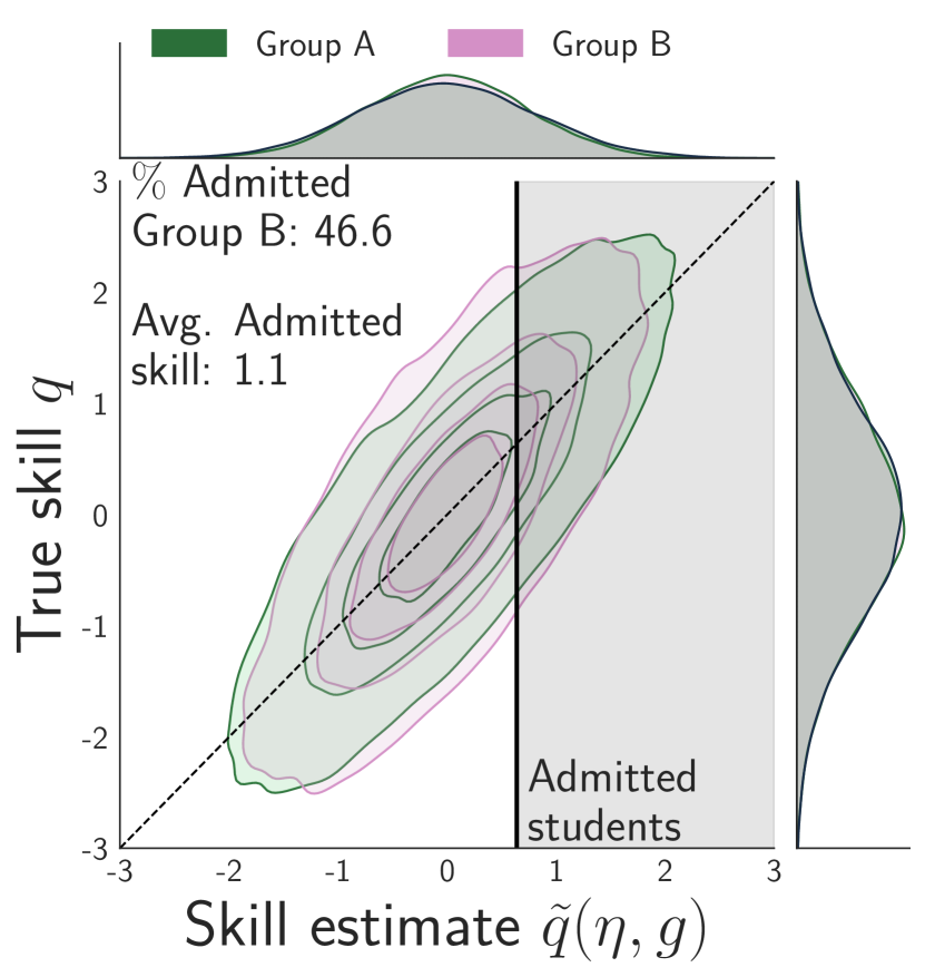
(a) With test, assume no barriers

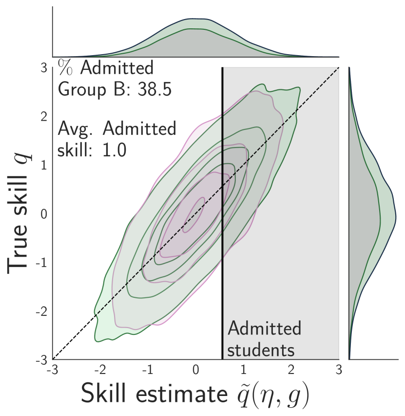
(b) With test, inaccessible to some

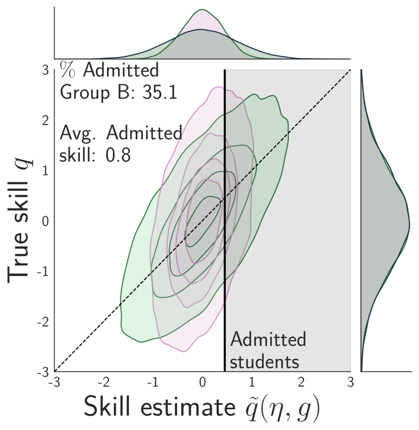
(c) Without test

Figure 2: Skill vs estimate joint distribution for each group. Above and to the right of each joint distribution we plot the corresponding marginal distributions – for example, the plot on the right of each joint distribution corresponds to the true skill distribution, which is equal across groups. The dashed diagonal lines correspond to perfect estimation. Figure 2(a) represents a world without access barriers and when the features are approximately equally informative across groups. Figure 2(b) illustrates the consequences of requiring a test when group B (in pink) has access barriers: fewer can apply and so can be admitted. Figure 2(c) illustrates potential consequences of dropping the test: the school may be unable to distinguish among group B applicants, leading to worse estimates (rotated away from diagonal) and fewer admitted from that group. Full model parameters, as for all figures, can be found in Online Appendix A.3.

Before proceeding to our main results, we first illustrate our primary insight regarding the trade-off between informativeness and the applicant pool size. In Figure 2, each sub-figure shows, for one scenario, the joint distribution between true skill $q$ and the corresponding skill estimates $\tilde{q}$ for each group – along with the respective marginal distributions. Since both groups have identical true skill distributions, the joint distributions would ideally be identical for the two groups (and perfectly aligned along the diagonal) and group $B$ would comprise a proportion $\pi$ of the admitted class.

Consider the case where the potentially dropped feature (the “test score”) is equally informative for both groups, whereas the remaining features are more informative for group $A$. Figure 2(a) illustrates the scenario when there are no access barriers to the test. Due to the differential informativeness induced by the other features, (slightly) more group $A$ students are admitted: the college can better estimate their true skill, as illustrated by the group $A$ joint distribution being closer to the diagonal. Figure 2(b) illustrates the consequences of requiring test scores in the presence of unequal access levels ($\gamma_{A}=1$ and $\gamma_{B}=\frac{2}{3}$). Among those who apply, the college can estimate true skill as well as it could in Figure 2(a). However, fewer group $B$ students can apply, as indicated by the smaller marginal count histogram, and so fewer are admitted. Figure 2(c) illustrates a scenario where the school removes the test score. Estimates for both groups are worse, as reflected in the joint distributions being further from the perfect estimation diagonal. However, skill estimates for group $B$ students are especially degraded as their other features may be less informative, and so they make up a smaller proportion of the admitted class. Whether the effect in Figure 2(b) or 2(c) dominates depends on the parameter context.

4 Analysis of the baseline model

In this section, we apply the insights from Section 3 on feature informativeness and skill estimation to our college admissions setting.

In Section 4.1, we focus solely on the effect of differences in informativeness, assuming no access barriers. We find that disparities arise with respect to all of our metrics of interest: academic merit, diversity, and individual fairness.

In Section 4.2, we compare two admissions policies: with and without a certain feature (e.g., test scores). When students have full and equal access to testing, we demonstrate how removing information might further decrease both fairness and academic merit under reasonable conditions. However, when students have different levels of access to the test, there is a trade-off between the barriers imposed by the test and the potentially valuable information the test may contain. We characterize the school’s optimal policy to include or exclude the test, depending on the relative sizes of these two effects.

(Beyond the study of the above baseline setting, in Section 5 and Section 5.2, we extend our model to contain strategic students and multiple schools. Finally, in Section E, we study the effect of affirmative action alongside the aforementioned policies.)

4.1 Informational effects of fixed testing policies

In general, our fairness notions are not achievable – even though we assume that both groups have the same true skill distributions. In the proposition below, we formalize the heterogeneous effects of differential informativeness on our three fairness metrics of interest. Note that for differential access barriers, this result would immediately follow from the definitions: high-skilled group $B$ students who otherwise would be admitted can no longer apply.

Recall from Section 2 that $\tilde{q}^{*}_{S}$ denotes the admission threshold of the school under policy $P_{S}$. Let also $\Phi$ denote the CDF of the standard Normal distribution $\operatorname{\mathcal{N}}(0,1)$.

Proposition 1 (Metrics with a fixed policy).

Suppose that a selective school uses admissions policy $P_{S}$. Group fairness and individual fairness fail except for equal precision, even without the presence of barriers. Given unequal precisions:

• Diversity level: Group $B$ students are under-represented, i.e., $\tau(P_{S})<\pi$.

  Furthermore, larger informativeness gap leads to decreased diversity: fix group B precision, $\sum_{k\in S}\sigma_{Bk}^{-2}$; then as group A precision increases, the diversity level $\tau(P_{S})$ decreases.

• Individual fairness: High-skilled group $B$ students are hard to target, i.e., $I(q;P_{S})>0$, if and only if

  $$q>\tilde{q}^{*}_{S}+\frac{\sigma^{-2}(\tilde{q}^{*}_{S}-\mu)}{\sqrt{\sum_{k\in S}\sigma_{Bk}^{-2}}\sqrt{\sum_{k\in S}\sigma_{Ak}^{-2}}}.$$

  Increasing the informativeness gap increases the individual fairness gap for high-skilled students: fix group $B$ precision, $\sum_{k\in S}\sigma_{Bk}^{-2}$; then as group $A$ precision increases, $I(q;P_{S})$ increases for ${q>\mu+\sigma\Phi^{-1}(1-C)}$.

• Academic merit: The policy achieves worse academic merit for admitted students from group $B$.

At a high level, this result suggests that, although the school’s Bayesian-optimal decision-making process can eliminate bias from skill estimates in terms of mean differences (see Section 3), the informativeness gap—as quantified via the difference in the total precision across groups—induces disparities in the admission outcomes even of ex-ante identical groups of students. As Figure 3 illustrates, and as we prove in Online Appendix C.3, with overall equal precision (the vertical line) both groups are admitted according to their population fractions (here, $1-\pi=\pi=0.5$); however, all fairness metrics degrade as the gap in informativeness between the two groups increases. Access barriers (even if limited to one group) would have a similarly negative effect, albeit for a different reason: high-skilled students who otherwise would be admitted cannot even apply as they have not taken the test, cf. Hyman (2016).

The errors in estimation due to unequal precision affect not only the diversity of the class but also the academic merit of each admitted group. As parts (i) and (iii) establish, under unequal precisions and no other disparities, students from group $A$ admitted to selective colleges are not only admitted at a higher rate, but – in contrast to existing theoretical results (cf., Faenza et al. (2020)) – are also of higher true skill (on average) compared to the admitted students from group $B$. This discrepancy is due to the fact that the school fails to identify the high-skilled students from group $B$: part (ii) for individual fairness shows that high-skilled students in group $B$ are less likely to be admitted than they would if they were in group $A$.

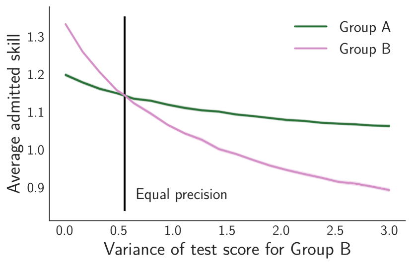
(a) Academic merit

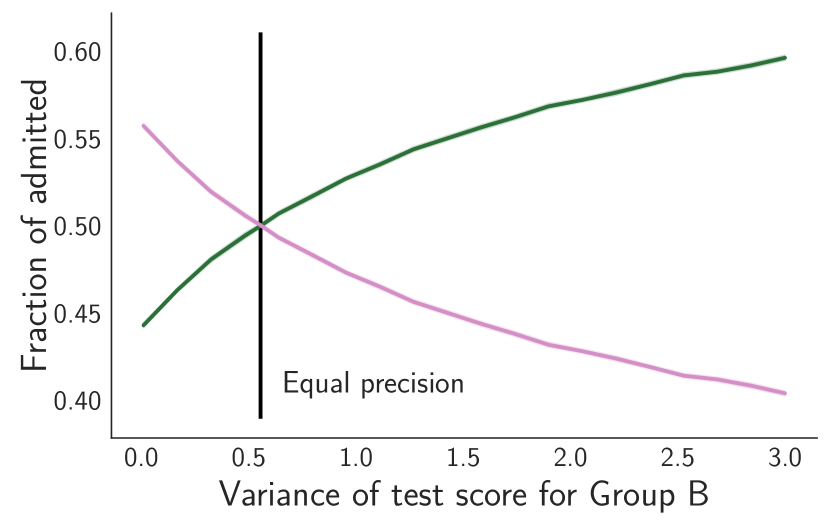
(b) Fraction of admitted students

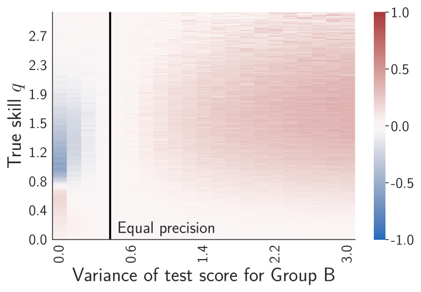
(c) Individual fairness gap

(d) Academic merit

(e) Fraction of admitted students

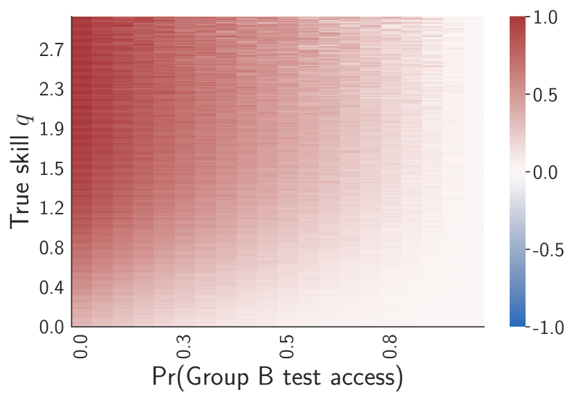
(f) Individual fairness gap

Figure 3: How the admitted students’ academic merit, fraction of each group, and individual fairness gap change with group $B$ test score variance and test access, respectively. Figures (a)-(c) fix test access $\gamma_{A}=\gamma_{B}=1$ and vary the test score variance. Figures (d)-(f) fix the test variance to be equal for both groups and vary test access $\gamma_{B}$. With equal precision and no barriers, groups are treated equitably. As the feature variance or barriers increase for group $B$, both academic merit of admitted $B$ students and fairness metrics worsen. We considered $\pi=1-\pi=0.5$; the full parameter set can be found in Online Appendix A.3.

We note that although the individual fairness gap is positive for all sufficiently high-skilled students, the magnitude of this gap varies. In fact, for students at the end of the right tail of the true skill distribution, the individual fairness gap starts to decrease, since – despite the noise – their estimates are high enough for admission. We prove this relationship in the following lemma.

Lemma 1.

Consider policy $P_{S}$, and assume unequal precision. The individual fairness gap $I(q;P_{S})$ is decreasing in $q$ for $q>q_{e}$, where

$$q_{e}\triangleq\tilde{q}^{*}_{S}+\sqrt{\frac{\sigma^{-4}(\mu-\tilde{q}^{*}_{S})^{2}}{{\sum_{k\in S}\sigma^{-2}_{Ak}}{\sum_{k\in S}\sigma^{-2}_{Bk}}}+\frac{\ln\left({{\sum_{k\in S}\sigma^{-2}_{Ak}}}\right)-\ln\left({{\sum_{k\in S}\sigma^{-2}_{Bk}}}\right)}{{\sum_{k\in S}\sigma^{-2}_{Ak}}-{\sum_{k\in S}\sigma^{-2}_{Bk}}}}.$$

Furthermore, $\lim_{q\rightarrow\infty}I(q;P_{S})=0$.

These results on how a single policy performs as the model parameters change further hint at the difficulty in deciding whether to drop standardized testing. Doing so increases estimation variance (perhaps differentially, as Bellafante (2020) and University of California Standardized Testing Task Force (2020) posit), worsening all metrics, but also reduces access barriers, improving all metrics. These effects interact to induce the overall effect. Our next section formalizes this interaction.

4.2 Dropping test scores with and without barriers

In this subsection, we ask: under what conditions would dropping a feature benefit the school and the applicants?. We study this question by comparing the test-free policy $P_{\operatorname{\textsc{sub}}}$ to the test-based policy $P_{\operatorname{\textsc{full}}}$ in two different scenarios: Theorem 1 and Theorem 2 consider settings with and without barriers, respectively.

Theorem 1 (Dropping tests with barriers).

Consider policies $P_{\operatorname{\textsc{full}}}$ and $P_{\operatorname{\textsc{sub}}}$ and assume unequal precisions under $P_{\operatorname{\textsc{full}}}$. In the presence of barriers, dropping test scores has the following implications:

• Diversity level: Holding other parameters fixed, there exists a threshold $\bar{\gamma}$ such that the diversity level improves under $P_{\operatorname{\textsc{sub}}}$ if and only if the fraction of group B students with access $\gamma_{B}<\bar{\gamma}$.

• Academic merit: For each group $g$, holding other parameters fixed, there exists a threshold $\bar{\bar{\gamma}}_{g}$ such that academic merit of group $g$ increases under $P_{\operatorname{\textsc{sub}}}$ if and only if $\gamma_{g}<\bar{\bar{\gamma}}_{g}$.

Perhaps surprisingly, Theorem 1 establishes that the academic merit of the admitted class may improve after dropping the test score. Similarly, diversity may deteriorate after dropping test scores. More specifically, Theorem 1 offers a threshold characterization, where the thresholds $\bar{\bar{\gamma}}_{g}$ and $\bar{\gamma}$ are functions of both the access levels of the two groups as well as the variance parameters, with and without the test. We provide the full characterization of these two quantities in Online Appendix C.5. We also include additional illustrations of the effects of dropping the test, with changes in the variance and access parameters.

At a high level, Theorem 1 implies that the decision to drop the test requirement is not just a matter of increasing access for the disadvantaged group. Rather, it depends on the complex interaction between the informational environment and the access levels of both groups. First, dropping test scores increases the applicant pool size but also affects its composition at different rates for each group. Second, the information loss incurred by dropping the test may not necessarily benefit students in group $B$. In particular, it is possible that the informational disadvantage faced by group $B$ students may be exacerbated by the absence of test score information even if test scores are more noisy for group $B$ than group $A$; especially when the testing barriers are relatively small, the negative informational effect may not be counterbalanced sufficiently by the increase in the group’s pool size.

In addition to the equivocal impact that dropping test scores can have on the diversity of the admitted class and the academic merit of each group, the decision to drop the test introduces some additional trade-offs. For example, as part (ii) in Theorem 1 implies and Figure 9 illustrates, it may be possible that one group’s admitted academic merit decreases, even if the overall academic merit increases. Depending on the exact model parameters, this might be an inevitable consequence of dropping the test score, raising interesting and important fairness trade-offs for policy-makers.

Our next result studies the role of information loss in more depth, focusing on just the effect of the variance parameters in a setting without access barriers.

Theorem 2 (Dropping tests without barriers).

Consider policies $P_{\operatorname{\textsc{full}}}$ and $P_{\operatorname{\textsc{sub}}}$, and assume unequal precisions under $P_{\operatorname{\textsc{full}}}$.

• Diversity level: Diversity level improves after dropping feature $K$, $\tau(P_{\operatorname{\textsc{sub}}})>\tau(P_{\operatorname{\textsc{full}}})$, if and only if

  $$\frac{\sum_{k\in\operatorname{\textsc{sub}}}\sigma_{Ak}^{-2}\left(\sigma^{-2}+\sum_{k\in\operatorname{\textsc{full}}}\sigma_{Ak}^{-2}\right)}{\sum_{k\in\operatorname{\textsc{sub}}}\sigma_{Bk}^{-2}\left(\sigma^{-2}+\sum_{k\in\operatorname{\textsc{full}}}\sigma_{Bk}^{-2}\right)}<\frac{\sigma^{-2}_{AK}}{\sigma_{BK}^{-2}}.$$ (3)

• Individual fairness: For each group $g$, there exist thresholds $q_{g}$ such that the admission probability for students of skill $q$ in group $g$ decreases under $P_{\operatorname{\textsc{sub}}}$ if and only if $q>q_{g}$. Further, there exists a threshold $\hat{q}\geq\max\{q_{A},q_{B}\}$ such that the individual fairness gap increases for all $q>\hat{q}$, but may decrease otherwise.

• Academic merit: Academic merit decreases for both groups $g\in\{A,B\}$, i.e.,

  $$\mathbb{E}[q\mid Y=1,g,P_{\operatorname{\textsc{full}}}]>\mathbb{E}[q\mid Y=1,g,P_{\operatorname{\textsc{sub}}}].$$

In the absence of barriers, the effect on the diversity level and individual fairness gap of dropping a feature depends on relative informativeness. However, it always worsens academic merit for both groups: without test scores, the school has access to fewer information signals and so skill estimates become noisier.

The exact effect on diversity depends on both the total precision of the remaining ${K-1}$ features and how much the test precisions $\sigma^{-2}_{A,K}$, $\sigma^{-2}_{B,K}$ differ. More specifically, Equation 3 is equivalent to the following condition

$$\frac{\left[\frac{\sum_{k\in\operatorname{\textsc{sub}}}\sigma_{Ak}^{-2}}{\sigma^{-2}+\sum_{k\in\operatorname{\textsc{sub}}}\sigma_{Ak}^{-2}}\right]}{\left[\frac{\sum_{k\in\operatorname{\textsc{sub}}}\sigma_{Bk}^{-2}}{\sigma^{-2}+\sum_{k\in\operatorname{\textsc{sub}}}\sigma_{Bk}^{-2}}\right]}<\frac{\left[\frac{\sum_{k\in\operatorname{\textsc{full}}}\sigma_{Ak}^{-2}}{\sigma^{-2}+\sum_{k\in\operatorname{\textsc{full}}}\sigma_{Ak}^{-2}}\right]}{\left[\frac{\sum_{k\in\operatorname{\textsc{full}}}\sigma_{Bk}^{-2}}{\sigma^{-2}+\sum_{k\in\operatorname{\textsc{full}}}\sigma_{Bk}^{-2}}\right]},$$ (4)

which intuitively encodes how informativeness for each group changes after dropping the test. If Equation 3 holds, then the diversity level improves as dropping the test narrows the relative informativeness gap between the two groups. However, if Equation 3 does not hold (as University of California Standardized Testing Task Force (2020) attests), removing test scores exacerbates the informational disadvantage of students in group $B$. In that case, dropping the test decreases diversity.

Similarly, dropping the test may worsen individual fairness. As part (ii) shows, the admission probability of students with sufficiently high true skill, for either group, decreases after removing the test. Furthermore, for sufficiently high-skilled students, the individual fairness gap increases after dropping test scores. This implication is separate from of the effect on overall diversity; although the school may manage to improve diversity by dropping the test, the targeting of high-skilled students in both groups becomes less effective, leaving high-skilled students in group $B$ disproportionately affected.

Even without access barriers, the result establishes the importance of understanding features other than the test score – not just their biases ($\mu_{gk}$, canceled out given full knowledge) but also their informativeness. More generally, our theoretical results illustrate that, even in a simple model, the debate over dropping standardized testing cannot be held without the particulars of the context: whether one cares about overall academic merit of the admitted class or our fairness criteria, the effects depend on the relationships between access barriers, the information content of the test, and the information content of other application components.

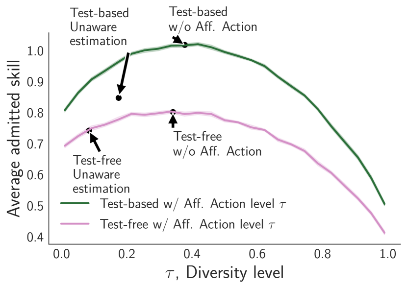
(a) Average admitted skill vs diversity level

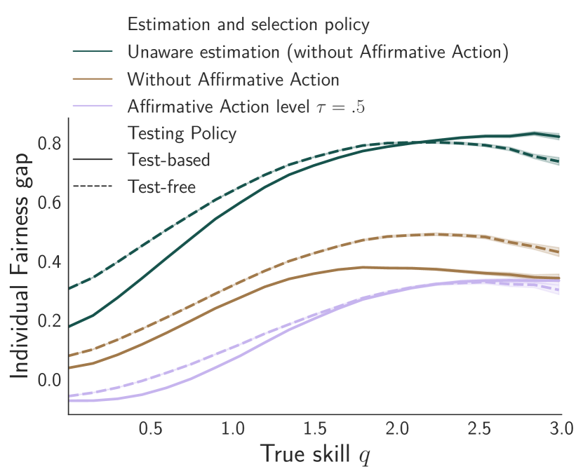
(b) Individual fairness gap

Figure 4: Performance of various policies – including group-unaware estimation policies, in setting where features are more informative for group $A$, and with testing barriers for group $B$. Affirmative action (discussed in Appendix E) in general improves both group diversity and individual fairness, while dropping the test score has an ambiguous impact. Group-unaware policies generally perform the worst on all metrics. The full parameter set can be found in Online Appendix A.3.

Comparing the policies in simulation. Figure 4 compares, for one parameter setting, our policies: with and without testing, and with and without affirmative action (where a fixed fraction $\tau$ of the admitted class is group B; see Section E). In Figure 4(a), the Pareto curves trace the trade-off between diversity and academic merit, for each testing policy. In this scenario, constraining each group’s admitted class to be proportional to its group size (affirmative action at level $\tau=\pi=\frac{1}{2}$) does not substantially affect academic merit, while improving both group and individual fairness substantially. Furthermore, dropping tests has an ambiguous effect: it worsens diversity levels and academic merit, as well as the individual fairness gap in the case without affirmative action. However, it (slightly) improves the individual fairness gap with affirmative action.

Figure 4 also includes group-unaware estimation policies, that ignore the social group that a student belongs to; in this case, estimating student skill levels requires calculating the posterior from a mixture of Normal distributions. Ignoring group attributes is an oft-proposed but often problematic policy proposal to combat bias (Corbett-Davies and Goel, 2018). Perhaps unsurprisingly, group-unaware estimation policies perform most poorly. It worsens both the average academic merit of the admitted class and the diversity level, compared to the policy with group-aware estimation. It also leads to large individual fairness gaps, especially for high-skilled students. More details can be found in Online Appendix A.1.

5 Extension: Strategic students

Above, we considered a scenario in which all students from a group $g$ share a common probability $\gamma_{g}$ of taking the test, independently of their true skill level. In this section, we incorporate student incentives: students who are more likely to be admitted if they take the test may be more willing to pay the cost to overcome barriers to taking the test or reporting their scores. To capture this effect, we introduce a model in which students face a (group dependent) cost to taking the test, that they weigh against their admissions probability conditional on taking the test. We then study how dropping the test affects diversity, merit, and individual fairness in this setting. Section 5.1 introduces and analyzes this model in a setting with a single school, and Section 5.2 extends this model to a setting with two schools, one of which requires the test. We compare effects with and without strategic students in Section 6, with data calibrated to real-world admissions data.

5.1 Single school

Before proceeding with the extended model, note that, in order to avoid confusion, in this section we will explicitly refer to $\tilde{q}_{\operatorname{\textsc{sub}}}\triangleq\tilde{q}(\operatorname{\bm{\theta}}_{\operatorname{\textsc{sub}}},g)$ and $\tilde{q}_{\operatorname{\textsc{full}}}\triangleq\tilde{q}(\operatorname{\bm{\theta}}_{\operatorname{\textsc{full}}},g)$ as skill estimates using those respective feature sets, instead of using the generic notation $\tilde{q}$ for the skill estimate.

Model and equilibria. We extend the model in Section 2 as follows. Each student in group $g$ incurs a constant cost $c_{g}$ to take the test. Admission to the school is of utility $v$. Students are strategic in the sense that they decide whether to apply to the school; $\alpha\in\{0,1\}$ denotes the action of the student, where $\alpha=0$ corresponds to not applying to the school and $\alpha=1$ corresponds to applying to the school. If the school uses a test-free policy, then all students apply ($\alpha=1$) without taking the test. If a school requires the test, then $\alpha=1$ corresponds to taking the test and applying (and thus paying the cost), and $\alpha=0$ to not taking the test. To rule out trivial equilibria where no students take the test due to high testing costs, we assume that the cost-to-valuation ratio $c_{g}/v<1$.

We assume that each student does not know their own true skill $q$, but does know their other features. Conditional on the other $K-1$ features $\operatorname{\bm{\theta}}_{\operatorname{\textsc{sub}}}$, the student wishes to maximize their expected utility. This expected utility depends on the valuation $v$ from getting admitted to the school with policy $P_{\operatorname{\textsc{full}}}$, the probability of being admitted, and the testing cost $c_{g}$. A student who does not apply to the school or is not admitted receives an outside option which we normalize to utility 0. Thus, for a school with policy $P_{\operatorname{\textsc{full}}}$, the student solves

$$\alpha(\operatorname{\bm{\theta}}_{\operatorname{\textsc{sub}}},g;P_{\operatorname{\textsc{full}}})=\arg\max_{\alpha\in\{0,1\}}\alpha\left(v\operatorname{\mathbb{P}}_{\theta_{K}}(Y=1\mid\operatorname{\bm{\theta}}_{\operatorname{\textsc{sub}}},g,P_{\operatorname{\textsc{full}}})-c_{g}\right).$$ (5)

If a school does not require the test ($P_{\operatorname{\textsc{sub}}}$), then the student always applies, i.e., $\alpha(\operatorname{\bm{\theta}}_{\operatorname{\textsc{sub}}},g;P_{\operatorname{\textsc{sub}}})=1$ for all $\operatorname{\bm{\theta}}_{\operatorname{\textsc{sub}}}\in\mathbb{R}^{K-1}$, $g\in\{A,B\}$.

The school’s admissions process is identical to before. The school maximizes the academic merit of the admitted class (without affirmative action), an objective that is strictly increasing in the skill estimate $\tilde{q}_{S}$. Therefore, it suffices to consider threshold-based selection policies $Y\in\{0,1\}$ that determine the lowest skill estimate $\tilde{q}^{*}_{S}$ that guarantees admission conditional on the student’s features $\operatorname{\bm{\theta}}_{S}$, group $g$, and test policy $P_{S}$, i.e., selection policies of the form $Y(\operatorname{\bm{\theta}}_{S},g;P_{S})=\operatorname{\mathbf{1}}\{\tilde{q}(\operatorname{\bm{\theta}}_{S},g)\geq\tilde{q}^{*}_{S}\}$. Thus, the optimal admission threshold is the point at which the mass of students admitted is equal to the school capacity:

$$\begin{split}\tilde{q}^{*}_{S}=\min\left\{z\in\mathbb{R}:\sum_{g}\pi_{g}\operatorname{\mathbb{E}}_{\operatorname{\bm{\theta}}_{S}}[\alpha^{*}(\operatorname{\bm{\theta}}_{\operatorname{\textsc{sub}}},g;P_{S})\mid\tilde{q}(\operatorname{\bm{\theta}}_{S},g)\geq z,g,P_{S}]\leq C\right\}.\end{split}$$ (6)

For a school with policy $P_{\operatorname{\textsc{sub}}}$, Equation 6 reduces to the baseline setting studied in the previous section (see Proposition 1). For policy $P_{\operatorname{\textsc{full}}}$, however, students become strategic, and thus we require a notion of equilibrium that impacts the school’s threshold policy. This equilibrium is formally defined as follows: Given test policy $P_{\operatorname{\textsc{full}}}$ and capacity $C$, we say that a pair $(\alpha^{*},Y^{*})$ constitutes an equilibrium if: (i) for all $\operatorname{\bm{\theta}}_{\operatorname{\textsc{sub}}}\in\mathbb{R}^{K-1}$ and $g\in\{A,B\}$, $\alpha^{*}(\operatorname{\bm{\theta}}_{\operatorname{\textsc{sub}}},g;P_{\operatorname{\textsc{full}}})=\arg\max_{\alpha\in\{0,1\}}\alpha\left(v\operatorname{\mathbb{P}}(Y^{*}=1\mid\operatorname{\bm{\theta}}_{\operatorname{\textsc{sub}}},g;P_{\operatorname{\textsc{full}}})-c_{g}\right)$; and (ii) for all $\operatorname{\bm{\theta}}_{\operatorname{\textsc{full}}}\in\mathbb{R}^{K}$ and $g\in\{A,B\}$, $Y^{*}(\operatorname{\bm{\theta}}_{\operatorname{\textsc{full}}},g;P_{\operatorname{\textsc{full}}})=\operatorname{\mathbf{1}}\{\tilde{q}(\operatorname{\bm{\theta}}_{\operatorname{\textsc{full}}},g)\geq\tilde{q}^{*}_{\operatorname{\textsc{full}}}\}$, where $\tilde{q}^{*}_{\operatorname{\textsc{full}}}$ is the corresponding solution to Equation 6.

The above definition of equilibria depends on the full vector of $K-1$ feature values $\operatorname{\bm{\theta}}_{\operatorname{\textsc{sub}}}$. However, as formalized in Lemma 11 in Online Appendix C.6, we can equivalently focus solely on the set of student actions that are dependent on $\tilde{q}_{\operatorname{\textsc{sub}}}$ instead of the entire vector of $K-1$ feature values $\operatorname{\bm{\theta}}_{\operatorname{\textsc{sub}}}$. We thus work directly with the reduced-form equilibrium $(\alpha(\tilde{q}_{\operatorname{\textsc{sub}}},g;P_{\operatorname{\textsc{full}}}),Y(\tilde{q}_{\operatorname{\textsc{full}}};P_{\operatorname{\textsc{full}}}))$. The next lemma establishes the existence and uniqueness of equilibria under test policy $P_{\operatorname{\textsc{full}}}$. Additionally, it demonstrates that students adhere to a threshold-based strategy at this equilibrium: only students with higher skill estimates $\tilde{q}_{\operatorname{\textsc{sub}}}$ opt to take the test.

Lemma 1.

Suppose that the school uses a test-based policy $P_{\operatorname{\textsc{full}}}$. There exists a unique equilibrium $(\alpha^{*},Y^{*})$, with the following property: there is a threshold $\underline{q}_{\operatorname{\textsc{sub}}}^{g}$ such that students in group $g$ take the test ($a=1$) if and only if $\tilde{q}_{\operatorname{\textsc{sub}}}\geq\underline{q}_{\operatorname{\textsc{sub}}}^{g}$, where

$$\underline{q}_{\operatorname{\textsc{sub}}}^{g}=\tilde{q}_{\operatorname{\textsc{full}}}^{*}-\Phi^{-1}\left(1-\frac{c_{g}}{v}\right)\left(\frac{\sigma_{gK}^{-2}}{\sigma^{-2}+\sum_{k\in\operatorname{\textsc{full}}}\sigma_{gk}^{-2}}\right)\sqrt{\sigma^{2}_{gK}+\frac{1}{\sigma^{-2}+\sum_{k\in\operatorname{\textsc{sub}}}\sigma_{gk}^{-2}}},$$ (7)

and $\tilde{q}^{*}_{\operatorname{\textsc{full}}}$ is the solution to Equation 6 so that $Y^{*}(\tilde{q}_{\operatorname{\textsc{full}}};P_{\operatorname{\textsc{full}}})=\operatorname{\mathbf{1}}\{\tilde{q}_{\operatorname{\textsc{full}}}\geq\tilde{q}^{*}_{\operatorname{\textsc{full}}}\}$.

Students do not know their own true skill $q$ but instead use their current skill estimate $\tilde{q}_{\operatorname{\textsc{sub}}}$ to assess the probability of attaining a test score high enough for admission to the school. If their perceived probability of admission is sufficiently high to outweigh the cost of the test, they decide to take the test and apply to the school. Several observations should be noted. First, in contrast to the non-strategic setup with access barriers of Theorem 1 where all students had the same a priori probability of being eligible to apply to the school, the decision to apply now correlates with the true skill level of each individual student, via the other features (see Figure 5). These selection effects change the composition of the applicant pool. Second, applying to the school does not guarantee admission. Conditional on $\alpha=1$, the higher the true skill (and thus the skill estimate $\tilde{q}_{\operatorname{\textsc{sub}}}$) of an applicant, the greater their probability of admission becomes. Nevertheless, a fraction of students will incur the test cost $c_{g}$, apply to the school, but ultimately be rejected. Third, similar to Theorem 1, a subset of non-applying students with skill estimates $\tilde{q}_{\operatorname{\textsc{sub}}}<\underline{q}_{\operatorname{\textsc{sub}}}^{g}$ would be admitted if taking the test were costless. The difference from Theorem 1 lies in the presence of self-selection bias among strategic students: in Lemma 1, students with $\tilde{q}_{\operatorname{\textsc{sub}}}<\underline{q}_{\operatorname{\textsc{sub}}}^{g}$ choose to not apply due to high test costs, whereas in Theorem 1, a fraction of students are exogenously excluded from access to the test, independently of their $\tilde{q}_{\operatorname{\textsc{sub}}}$.

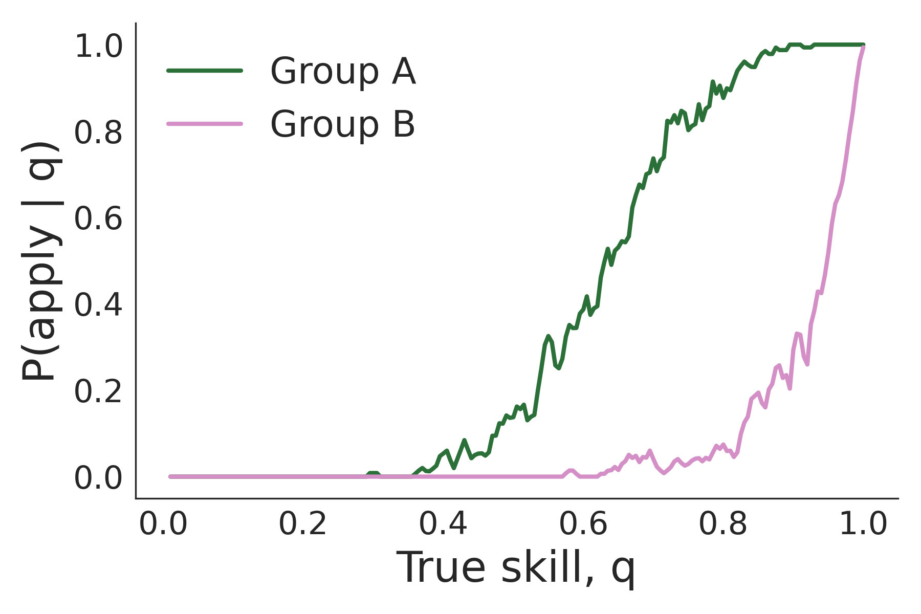
Figure 5: When students are strategic, high skilled students are more likely to take the test and apply. We consider a case where Group $A$ has higher precision and lower test costs: Parameters are $\mu_{gk}=0$ for all $g,k$, $\sigma^{2}_{A1}=\sigma^{2}_{A2}=\sigma^{2}_{B1}=1$ and $\sigma^{2}_{B2}=2$, where $k=2$ denotes the test feature. Costs are $c_{A}=0.5$ and $c_{B}=3$. Full parameter set can be found in Online Appendix B.2.

A special case that illustrates the effect of test costs and information on student behavior is when test costs are equal ($c_{A}=c_{B}$), precisions are equal for the first $K-1$ features, and group $A$ has more informative test scores than group $B$ ($\sigma_{AK}^{2}<\sigma^{2}_{BK}$). Under these conditions, at the time of application, both groups share the same observable characteristics, $c_{g}/v$ and $\tilde{q}_{\operatorname{\textsc{sub}}}$. However, the uncertainty about their test scores impacts their behavior differently. A test with high precision means that the school places high importance on the test information (see Equation 1), which is currently unknown to the students at the time of making the testing decision. Thus, the admissions decision will rest on the (unknown) test score. How does this increased importance affect the student’s testing decision? The cost-to-valuation ratio appears to function as a risk-adjusting device in conjunction with the test informativeness. Fix $\tilde{q}^{*}_{\operatorname{\textsc{full}}}$; as implied by Corollary 3 in Online Appendix C.6, if $c_{g}/v<0.5$, then $\underline{q}_{\operatorname{\textsc{sub}}}^{A}<\underline{q}_{\operatorname{\textsc{sub}}}^{B}$, indicating that more students from group $A$ are willing to accept a higher risk of rejection and apply at a greater rate than group $B$. The opposite holds true when $c_{g}/v>0.5$. In both cases, note that the value of $c_{g}/v$ has no direct effect on the actual admissions probabilities but nevertheless influences the candidates’ pool through the students’ self-selection bias.

Moving from individual student behavior to admissions outcomes, we now analyze the interplay between test cost and informativeness at the unique equilibrium under $P_{\operatorname{\textsc{full}}}$.

Effect of test cost and informativeness on admissions. In the non-strategic setting of Proposition 1, we found that the sign of the informativeness gap, measured by the difference $\sum_{k\in S}\sigma^{-2}_{Ak}-\sum_{k\in S}\sigma^{-2}_{Bk}$, determined the diversity level and academic merit in a straightforward manner: if group $B$ has lower total precision than group $A$, then it is under-represented and has lower academic merit among the admitted class. The same holds even in the presence of barriers as long as $\gamma_{A}\geq\gamma_{B}$. However, when the test is costly, Proposition 2 below shows that the relationship between informativeness and fairness becomes more complex, depending on the costs and informativeness of the features with and without the test score. (Recall that $\Phi_{2}(x,y;\rho)$ denotes the CDF of the standard bivariate Normal distribution with correlation $\rho$.)

Proposition 2.

Consider the equilibrium under policy $P_{\operatorname{\textsc{full}}}$.

• Diversity level: Group $B$ students are under-represented, i.e., $\tau(P_{\operatorname{\textsc{full}}})<\pi$, if and only if

  $$\frac{\Phi\left(\frac{\alpha_{A}+b_{A}\mu}{\sqrt{1+\tilde{\sigma}_{A}^{2}b_{A}^{2}}}\right)-\Phi_{2}\left(\frac{\alpha_{A}+b_{A}\mu}{\sqrt{1+\tilde{\sigma}_{A}^{2}b_{A}^{2}}},\frac{\tilde{q}^{*}_{\operatorname{\textsc{full}}}-\mu}{\tilde{\sigma}_{A}};-\frac{\tilde{\sigma}_{A}b_{A}}{\sqrt{1+\tilde{\sigma}_{A}^{2}b_{A}^{2}}}\right)}{\Phi\left(\frac{\alpha_{B}+b_{B}\mu}{\sqrt{1+\tilde{\sigma}_{B}^{2}b_{B}^{2}}}\right)-\Phi_{2}\left(\frac{\alpha_{B}+b_{B}\mu}{\sqrt{1+\tilde{\sigma}_{B}^{2}b_{B}^{2}}},\frac{\tilde{q}^{*}_{\operatorname{\textsc{full}}}-\mu}{\tilde{\sigma}_{B}};-\frac{\tilde{\sigma}_{B}b_{B}}{\sqrt{1+\tilde{\sigma}_{B}^{2}b_{B}^{2}}}\right)}>\frac{\tilde{\sigma}_{B}}{\tilde{\sigma}_{A}},$$ (8)

  where the full definitions of $\tilde{\sigma}_{g}$, $a_{g}\triangleq a_{g}(\tilde{q}_{\operatorname{\textsc{full}}}^{*})$, $b_{g}\triangleq b_{g}(\tilde{q}^{*}_{\operatorname{\textsc{full}}})$ can be found in Online Appendix C.6.

• Academic merit: Policy $P_{\operatorname{\textsc{full}}}$ achieves worse academic merit for group $B$ if and only if $\lambda(a_{A},b_{A},\tilde{\sigma}_{A},\tau_{A})>\lambda(a_{B},b_{B},\tilde{\sigma}_{B},\tau_{B}),$ where

  $$\begin{split}\lambda(a_{g},b_{g},\tilde{\sigma}_{g},\tau_{g})\triangleq\frac{\mu}{\tilde{\sigma}_{g}}&-\frac{\tilde{\sigma}_{g}^{2}b_{g}}{\tau_{g}\sqrt{1+\tilde{\sigma}_{g}^{2}b_{g}^{2}}}\phi\left(\frac{a_{g}+b_{g}\mu}{\sqrt{1+\tilde{\sigma}_{g}^{2}b_{g}^{2}}}\right)\Phi\left(\tilde{q}^{*}_{\operatorname{\textsc{full}}}\sqrt{1+\tilde{\sigma}_{g}^{2}b_{g}^{2}}+\frac{b_{g}\tilde{\sigma}_{g}(a_{g}+b_{g}\mu)}{\sqrt{1+\tilde{\sigma}_{g}^{2}b_{g}^{2}}}\right)\\ &+\Phi(a_{A}+b_{g}\mu+b_{g}\tilde{\sigma}_{g}\tilde{q}^{*}_{\operatorname{\textsc{full}}})\frac{\phi(\tilde{q}^{*}_{\operatorname{\textsc{full}}})}{\tau_{g}}.\end{split}$$

Observe that admissions decisions (and thus diversity and academic merit) now depend not only on the overall feature informativeness, but separately on the informativeness of the test score and other $K-1$ features and the cost-to-valuation ratio $c_{g}/v$. There are several mechanisms that might lead to high diversity—that is, group $B$ representation over their population fraction $\pi$—even if we assume unequal precisions under policy $P_{\operatorname{\textsc{full}}}$ and higher test costs for group $B$ than group $A$. For example, one possible mechanism is that, due to the strategic behavior of students, the applicant pool composition is significantly skewed towards group $B$. The intuition stems again from Lemma 1. Differences in the cost-to-valuation ratio and test informativeness across groups (even in favor of group $A$) might lead students with equal skill estimates $\tilde{q}_{\operatorname{\textsc{sub}}}$ but from different groups to take different actions depending on the value of $\underline{q}^{g}_{\operatorname{\textsc{sub}}}$ thus making group $B$ apply at a greater rate than group $A$ in some instances. Another mechanism is that, even if students from both groups self-select to apply at similar rates, the test score could be significantly more informative for group $B$ than $A$, thus a highly selective school is able to distinguish the high-skilled group $B$ students (among the already high-skilled applicant pool) more efficiently than group $A$ students.

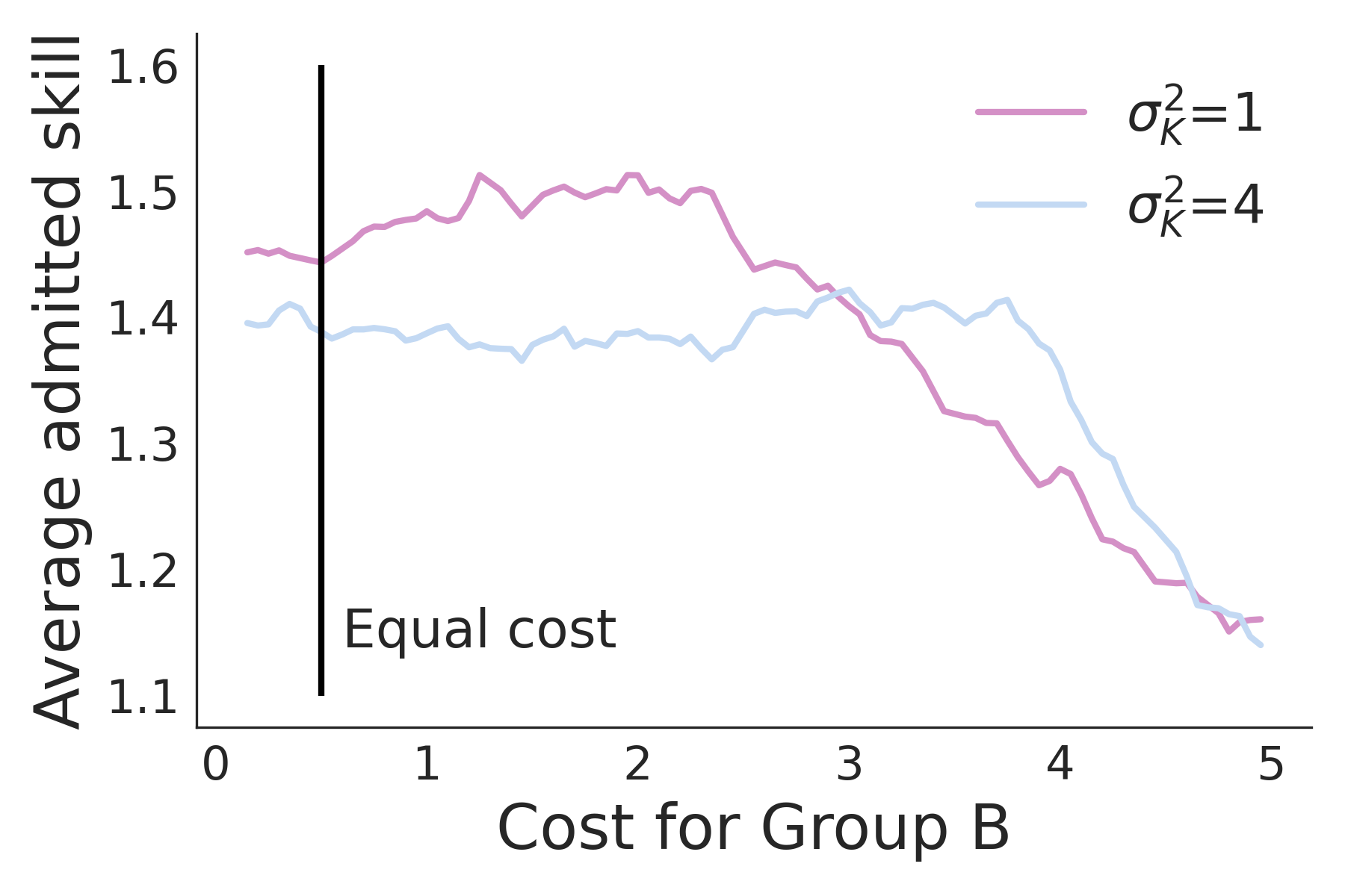
(a) Academic merit

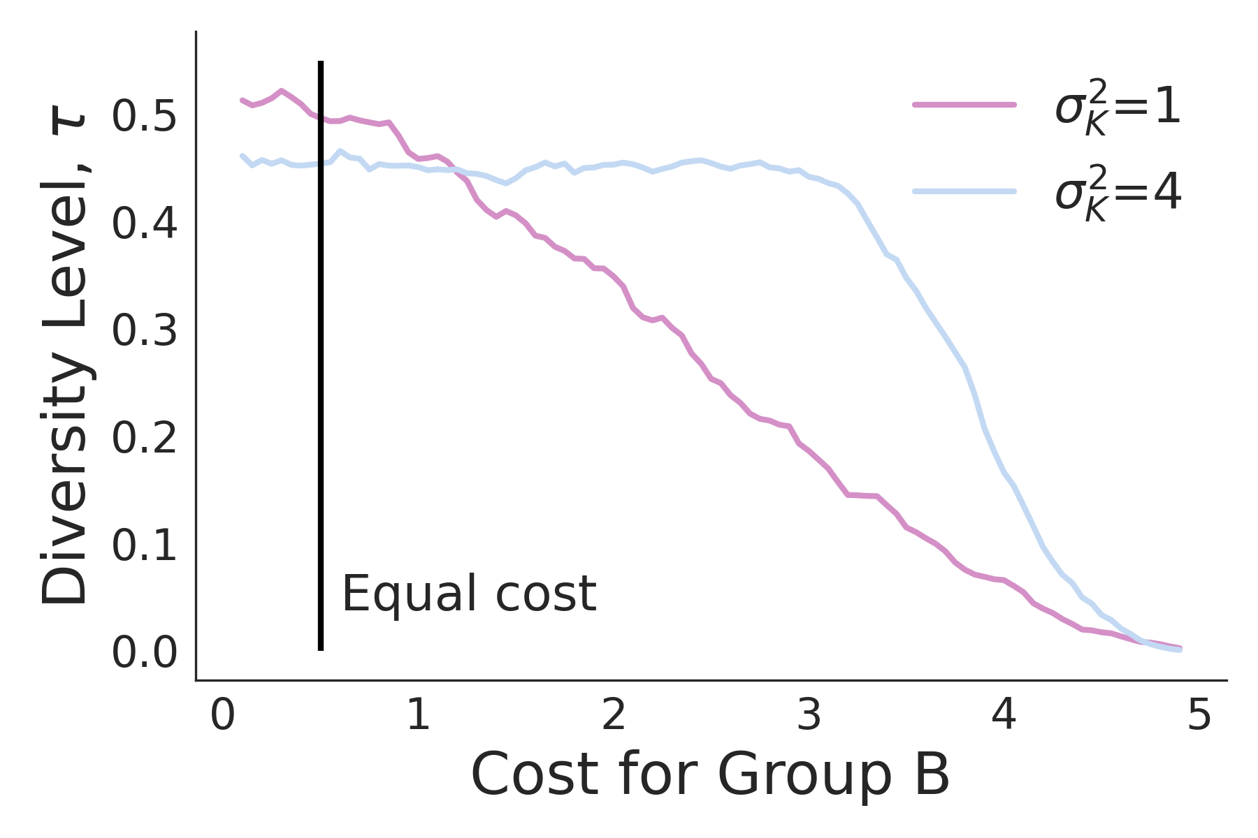
(b) Diversity level

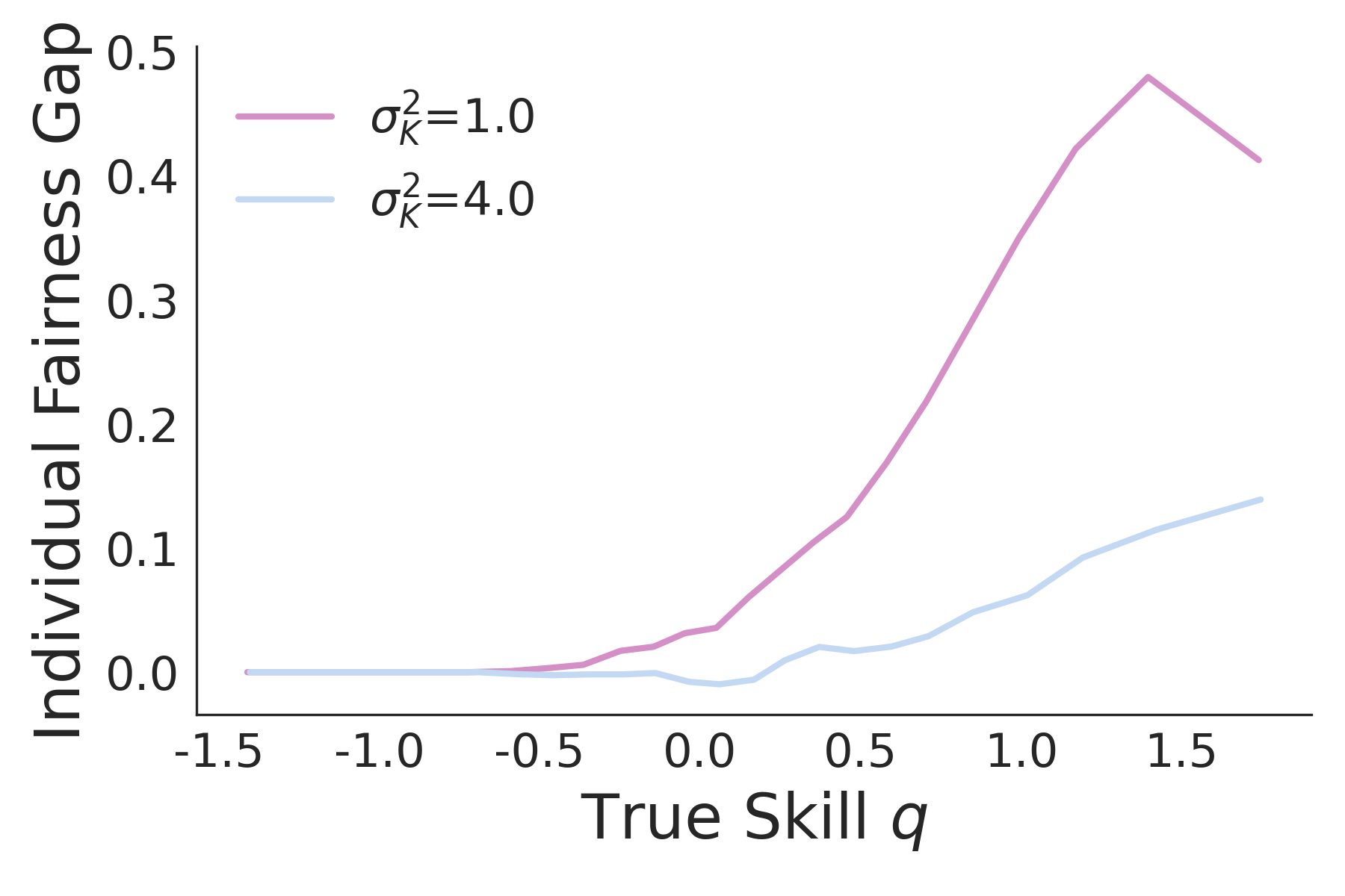
(c) Individual fairness gap

Figure 6: Strategic students setting. How the admitted students’ academic merit, diversity level, and individual fairness gap depend on test informativeness $\sigma^{2}_{K}$ for Group $B$. Figures 6(a) and 6(b) fix cost $c_{A}=0.5$ and vary $c_{B}$. Academic merit and diversity are particularly harmed when the test is costly and informative for Group $B$. Figure 6(c) considers a fixed cost $c_{B}=3$ and shows that individual fairness is worse when the test is more informative for Group $B$. Full parameter set can be found in Appendix B.2.

Figure 6 explores the interactions between test informativeness and test costs on academic merit, diversity, and individual fairness. Figures 6(a) and 6(b) show that high test costs for Group $B$ can negatively affect both the academic merit and diversity levels, respectively, of the admitted student body. In particular, when test costs are high for group $B$, academic merit and diversity are worse when the test feature variance is $\sigma^{2}_{B2}=1$ than when $\sigma^{2}_{B2}=4$. In other words, when the test cost is high, the exclusionary nature of the test is particularly harmful when the test is more informative (lower conditional variance). This result follows from the fact that fewer students risk taking the test when it is more informative (i.e., more self-select out of taking it).

5.2 Two schools

We consider a setting with two schools $J_{1}$, $J_{2}$ with respective capacities $C_{1}$, $C_{2}$ such that the market is over-demanded, i.e., $C_{1}+C_{2}<1$. Let $P_{S}^{i}$ denote the test policy of school $i\in\{1,2\}$. Here we assume that school $J_{1}$ uses a test-based policy $P^{1}_{\operatorname{\textsc{full}}}$ while school $J_{2}$ uses a test-free policy $P^{2}_{\operatorname{\textsc{sub}}}.$ For brevity, define $\mathbf{P}=(P^{1}_{\operatorname{\textsc{full}}},P^{2}_{\operatorname{\textsc{sub}}})$. Students in both groups have higher valuation for $J_{1}$ than $J_{2}$, i.e., $v_{1}>v_{2}$. They may decide to apply to zero, one or both schools. Analogous to above, to eliminate trivial equilibria we assume $c_{g}/(v_{1}-v_{2})<1$. As in Section 5.1, if a school uses policy $P_{\operatorname{\textsc{full}}}$, only students who take the test are eligible.

We extend the definition of (reduced-form) equilibria to this setting with two schools. First, we consider the schools’ selection policies. Let $Y_{i}(\tilde{q}_{S},g;\mathbf{P})$ denote the selection policy of school $J_{i}$ and define $\mathbf{Y}=(Y_{1},Y_{2})$; analogously to the case of one school, each $Y_{i}$ remains well-defined. At an equilibrium $(\alpha,\mathbf{Y})$, given the student preferences, the more preferred school $J_{1}$ picks students first and optimizes the academic merit of the admitted class. Similarly, $J_{2}$ optimizes academic merit by selecting among the students who either did not apply to $J_{1}$ at all or applied but did not get admitted. Online Appendix C.7 contains the characterization of the optimization functions for both schools and Lemma 12 formalizes that each $Y_{i}$ preserves its threshold-based form.

Next, we consider the students’ action $\alpha$. Note that, a student always has an incentive to apply to the test-free school $J_{2}$. Thus, the student must decide whether they also want to apply to $J_{1}$ by solving the following optimization problem:

$$\alpha(\tilde{q}(\operatorname{\bm{\theta}}_{\operatorname{\textsc{sub}}},g),g;\mathbf{P})=\arg\max_{\alpha\in\{0,1\}}\alpha\left(v_{1}\operatorname{\mathbb{P}}(Y_{1}=1\mid\operatorname{\bm{\theta}}_{\operatorname{\textsc{sub}}},g,P^{1}_{\operatorname{\textsc{full}}})-c_{g}\right)+v_{2}\operatorname{\mathbb{P}}(Y_{1}=0\cap Y_{2}=1\mid\operatorname{\bm{\theta}}_{\operatorname{\textsc{sub}}},g,{P}^{2}_{\operatorname{\textsc{sub}}}).$$

If the student applies to both schools and is also admitted to both, they go to school $J_{1}$.

This optimization problem induces more complex application behavior than in the single school case, which we discuss in Theorem 3 and Figure 7.

Theorem 3.

Consider the setting with two schools defined above. Then, there exists a unique equilibrium $(\alpha^{*},\mathbf{Y}^{*})$ with the following properties:

• School $J_{i}$’s selection policy $Y^{*}_{i}$ takes a threshold form: $Y^{*}_{i}(\tilde{q}_{S};\mathbf{P})=\operatorname{\mathbf{1}}\{\tilde{q}_{s}\geq\tilde{q}^{*}_{i}\}$, where $\tilde{q}^{*}_{i}$ is school $J_{i}$’s admission threshold.

• Students in group $g$ take the test and apply to school $J_{1}$, if and only if one of the following conditions holds:

  • either $\tilde{q}^{*}_{2}>\tilde{q}_{\operatorname{\textsc{sub}}}\geq\underline{q}_{l}^{g}$ where

    $$\underline{q}_{l}^{g}=\tilde{q}_{1}^{*}-\Phi^{-1}\left(1-\frac{c_{g}}{v_{1}}\right)\left(\frac{\sigma_{gK}^{-2}}{\sigma^{-2}+\sum_{k\in\operatorname{\textsc{full}}}\sigma_{gk}^{-2}}\right)\sqrt{\sigma^{2}_{gK}+\frac{1}{\sigma^{-2}+\sum_{k\in\operatorname{\textsc{sub}}}\sigma_{gk}^{-2}}};$$ (9)

  • or $\tilde{q}_{\operatorname{\textsc{sub}}}\geq\max\{\underline{q}_{h}^{g},\tilde{q}^{*}_{2}\}$, where

    $$\underline{q}_{h}^{g}=\tilde{q}_{1}^{*}-\Phi^{-1}\left(1-\frac{c_{g}}{v_{1}-v_{2}}\right)\left(\frac{\sigma_{gK}^{-2}}{\sigma^{-2}+\sum_{k\in\operatorname{\textsc{full}}}\sigma_{gk}^{-2}}\right)\sqrt{\sigma^{2}_{gK}+\frac{1}{\sigma^{-2}+\sum_{k\in\operatorname{\textsc{sub}}}\sigma_{gk}^{-2}}}.$$ (10)

  Furthermore, $\underline{q}_{l}^{g}<\underline{q}_{h}^{g}$ for both groups $g\in\{A,B\}$.

• Assume that $\tilde{q}^{*}_{2}>\underline{q}^{g}_{h}$. Then, school $J_{1}$ is more diverse than $J_{2}$ if and only if

  $$\begin{split}\tilde{\sigma}_{B}\Phi\left(\frac{\alpha_{B}+b_{B}\mu}{\sqrt{1+\tilde{\sigma}_{B}^{2}b_{B}^{2}}}\right)-\tilde{\sigma}_{B}\Phi_{2}\left(\frac{\alpha_{B}+b_{B}\mu}{\sqrt{1+\tilde{\sigma}_{B}^{2}b_{B}^{2}}},\frac{\tilde{q}^{*}_{1}-\mu}{\tilde{\sigma}_{B}};-\frac{\tilde{\sigma}_{B}b_{B}}{\sqrt{1+\tilde{\sigma}_{B}^{2}b_{B}^{2}}}\right)>\Phi\left(\frac{\tilde{q}^{*}_{2}-\mu}{\sigma\sqrt{\frac{\sum_{k\in\operatorname{\textsc{sub}}}\sigma_{gk}^{-2}}{\sigma^{-2}+\sum_{k\in\operatorname{\textsc{sub}}}\sigma_{gk}^{-2}}}}\right),\end{split}$$

  where $a_{g}=a_{g}(v_{1})$, $b_{g}=b_{g}(\tilde{q}^{*}_{1})$, and $\tilde{\sigma}_{g}$ are defined as in Proposition 2.

• There exist instances of the model parameters such that school $J_{1}$ achieves lower academic merit for group $g$ than $J_{2}$. See Online Appendix C.7 for a characterization.

The above theorem establishes several interesting properties at the equilibrium. Even this two-school setting induces complex student strategic behavior. Figure 7 illustrates the student test-taking behavior, described in Part (ii) above. In particular, student test-taking behavior is not necessarily a single threshold in their skill estimates $\tilde{q}_{\operatorname{\textsc{sub}}}$ using the first $K-1$ features. Some students with lower skill estimates $q_{\operatorname{\textsc{sub}}}$ (who, after observing the first $K-1$ features, know they will not be admitted to the test-free school $J_{2}$) take the test for a chance of admission to school $J_{1}$.

This discontinuity in the students’ application behavior potentially leads to a mismatch between the skill of the applicants and the ranking of the school. Even though – by Part (i) – schools continue to use admission cutoffs that are increasing in their ranking, students’ nonmonotonic behavior breaks the positive assortativeness property that matching models typically exhibit (Chade et al., 2017). This explains the existence of instances where school $J_{1}$ achieves lower academic merit than the less-preferred school $J_{2}$ (Part (iv)). Note that this phenomenon would not arise if both schools used the same testing policy since all students would apply to either none or both schools.

Finally, as Part (iii) shows, adopting different test policies across schools may lead to different levels of diversity across schools, although the theorem statement does not rule out the possibility that both schools suffer from low diversity. The intuition is similar to Proposition 2.

Figure 7: Students in group $g$ enrolled at schools $J_{1}$ and $J_{2}$. The left and right panel of the figure correspond to $\tilde{q}^{*}_{2}<\underline{q}_{h}^{g}$ and $\tilde{q}^{*}_{2}>\underline{q}_{h}^{g}$, respectively. In both cases, all students apply to $J_{2}$ but only the students with skill estimates above the cutoff $\tilde{q}^{*}_{2}$ get admitted to $J_{2}$. Among those students only the mass of students in the purple-shaded area will accept $J_{2}$’s offer, since a fraction of the students admitted to $J_{2}$ also applied and got admitted to $J_{1}$ (yellow area). However, as the left panel illustrates for $\tilde{q}^{*}_{2}<\underline{q}_{h}^{g}$, not all students who apply to $J_{2}$ necessarily apply to $J_{1}$ as well; indeed, the admitted students with $\tilde{q}^{*}_{2}\leq\tilde{q}_{\textrm{SUB}}<\underline{q}^{g}_{h}$ have applied only to $J_{2}$. Furthermore, observe that the students who successfully apply to $J_{1}$ (represented by the yellow-shaded area) are not always characterized by higher skill estimates than the admitted students at $J_{2}$. Finally, note that in both panels, all students with $\underline{q}_{l}^{g}<\tilde{q}^{*}_{2}$ applied to $J_{1}$, however only the yellow-shaded mass of students got admitted.

6 Calibrated simulations with UT Austin data

We calibrate our model to empirical data from the University of Texas at Austin to assess the effects of dropping test requirements under our model. Our results establish that (a) there are reasonable parameter ranges both in which dropping the test can be beneficial and harmful for the desiderata, and (b) when tests are required, outcomes can depend on whether the model allows students to self-select to take the test.

Data. Our data is from the Texas Higher Education Opportunity Project (THEOP), a semipublic dataset of applications and transcripts for universities in Texas (Tienda and Sullivan, 2011). We focus on data from the University of Texas at Austin, for students who applied in 1992-1997. For each applicant, we observe their high school class rank (rounded to nearest decile), standardized test score (SAT, or ACT score translated to equivalent SAT score); we also observe characteristics of their high school (including relative economic privilege rounded to nearest quartile, which is a measure of the socioeconomic status of the students the high school serves). We further observe admissions decisions and, for accepted students, whether they enrolled. Finally, for those who enrolled, we observe rich transcript data: their GPA and number of credit hours for each enrolled semester, that we use to calculate overall GPA in their first year and afterwards.

Calibration and simulation setup. We consider our applicant population as those who in reality enrolled to UT Austin (i.e., those for whom we observe college transcript data), and simulate a setting in which these applicants are further applying to a selective program, e.g., honors programs, scholarships, or college transfers. For each such individual, we use their cumulative college GPA – not counting their first year – to represent their true skill. Then, as features, we use (in various simulations) their high school class rank, standardized test score and/or college first-year GPA. To form the two groups, we take the upper (group $A$) and lower (group $B$) halves of the high schools’ economic privilege index.

We calibrate our model parameters to the empirical data. We calibrate the true skill mean $\mu$ and variance $\sigma^{2}$ to the empirical mean and variance of the cumulative college GPA, excluding the first year. We then calibrate the conditional feature distributions for each group, which in our model are distributed as $\theta_{k}\sim N(q+\mu_{gk},\sigma^{2}_{gk})$; i.e., for each group $g$ and feature $k$ pair, we need estimates of $\mu_{gk}$ and $\sigma^{2}_{gk}$, the conditional mean and variance of the feature given the student’s true skill. We estimate these values by running an ordinary least squares regression $\theta_{k}\sim q$, where $q$ is the observed college GPA. Let the fitted regression model be $\hat{\theta}_{k}=\hat{\beta}_{0}+\hat{\beta}_{1}q$, so that $q=(\hat{\theta}_{k}-\hat{\beta}_{0})/\hat{\beta}_{1}$. To normalize the features so that a one unit increase in the feature corresponds to a one unit increase in skill level (so that the feature has mean $q+\mu_{gk}$), we center and scale each observed feature to obtain $\theta_{k}^{\prime}=(\theta_{k}-\hat{\beta}_{0})/\hat{\beta}_{1}$, and likewise for the predicted features $\hat{\theta}_{k}$ to obtain $\hat{\theta}_{k}^{\prime}$. Now, we calibrate the model to the distribution of $\theta_{k}^{\prime}$. We set $\mu_{gk}$ to be the sample mean of $\theta_{k}^{\prime}$, which is 0, since $\theta_{k}^{\prime}$ is centered. Then, $\sigma^{2}_{gk}$ is the sample variance of the residuals $\hat{\theta}_{k}^{\prime}-\theta_{k}^{\prime}$. The calibrated variance parameters $\sigma^{2}_{gk}$ are in Table 1.

Group	HS class rank	College GPA, 1st year	Test score
A (high economic privilege)	1.84	0.77	2.60
B (low economic privilege)	3.27	0.86	2.14

Table 1: Calibrated feature variance $\sigma^{2}_{gk}$ for each group $g$ and feature $\theta_{k}$. This calibration suggests that class rank is relatively more predictive of cumulative college GPA for the high economic privilege group while the test score is more predictive for the low economic privilege group – consistent with University of California Standardized Testing Task Force (2020) and Schmill (2022). Most predictive for each is the first-year college GPA.

Using these calibrated mean and variance parameters, we then simulate our model, with the students’ applications and the school’s Bayesian updating as described earlier. We simulate the admission outcomes in both the setting with strategic students and the setting with non-strategic students. In both settings, we fix group $A$ to have full access to the test ($\gamma_{A}=1$ and $c_{A}=0$ in the non-strategic and strategic settings, respectively) and vary the level of access for group $B$ students. We fix an equal proportion of students from each group in the candidate pool ($\pi=0.5$). We simulate a setting with 10,000 applicants and a capacity of 1,000. For each parameter set, we run 100 simulations and report the mean and 95% confidence intervals across simulation runs.

We simulate two informational cases, which correspond to the school having access to different features when making its decision.

Low informativeness:

Class rank and (potentially) Test score. Simulates, for example, honors program decision being made for incoming first-year students.

High informativeness:

First-year GPA and (potentially) Test score. Simulates, for example, honors program decision being made after the first year.

To make the non-strategic and strategic settings comparable, we define the notion of test access level for group $B$ as the proportion of group $B$ students taking the test. In the non-strategic setting, this is $\gamma_{B}$ by definition. In the strategic setting, each cost level $c_{B}$ induces a test access level which can be found through simulation. We note that while the overall number of group $B$ students taking the test is the same for a fixed test access level, in the strategic setting this group of students are disproportionately high-skilled (see Lemma 1 and Figure 5).

		Academic merit		Diversity Level
Informational Case	Student behavior	With test	Without test	With test	Without test
Low	Strategic	3.72	3.54	46.4%	37.1%
	Non-strategic	3.64	3.54	26.6%	37.1%
High	Strategic	3.88	3.81	49.5%	48.2%
	Non-strategic	3.79	3.81	28.4%	48.2%

Table 2: How academic merit and diversity level of admitted students change with and without requiring a test score, for two informational cases (how informative the non-test feature is) and for the strategic and non-strategic settings. Academic merit (GPA) ranges from 1.0-4.0. Diversity level is shown as a percentage of admitted students. This table assumes a 40% test access for group $B$; for outcomes for the full range of group $B$ test access, see Figures 8 and 10. Values are averaged across 100 simulation runs and all differences are statistically significant; see Table 3 for 95% confidence intervals across simulation runs.

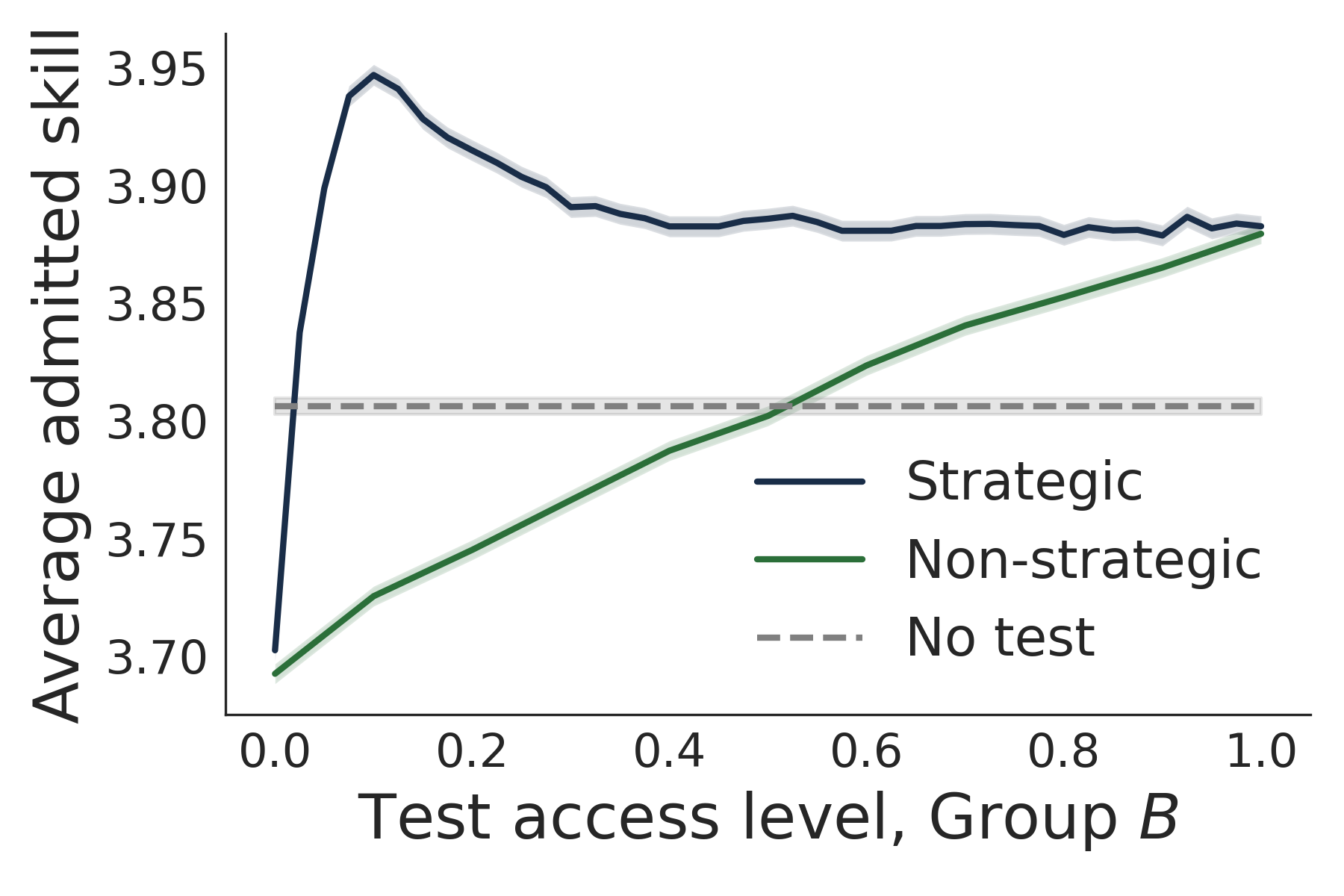
(a) Academic merit

(b) Diversity level

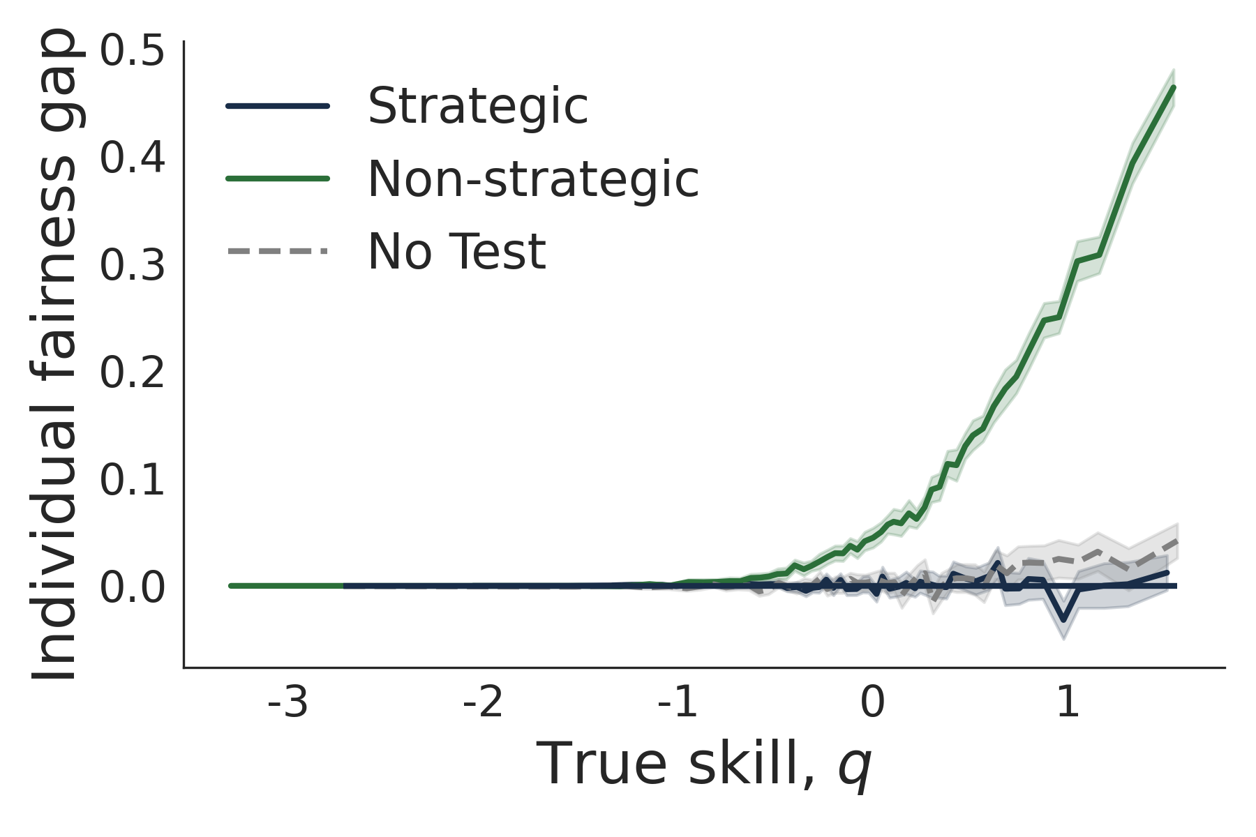
(c) Individual fairness gap

Figure 8: Calibrated simulations when full set of features is $\{$First year GPA, test score$\}$ – high informativeness case (see Table 1 for informativeness of features). Figures (8a) and (8b) vary test the access level for group $B$. Figure (8c) shows the individual fairness gap at a fixed group $B$ test access level of 40%. Figures show average value across 100 simulation runs and 95% confidence intervals.

Simulation results. Table 2 summarizes the admission outcomes with and without the test, for a fixed level of group $B$ students having access (40%), while all group $A$ students have access. For outcomes for the full range of group $B$ test access, see Figures 8 and 10, for the high and low informational environment, respectively.

In this setting, exactly half of the students are in group $B$ ($\pi=0.5$). For any diversity level below 50% (i.e., students in group $B$ make up less than half of the admitted student body), we consider group $B$ to be under-represented.

Overall, the results show that the effects of dropping the test requirement depend crucially on both the informational environment and whether students are strategic. At a test access level of 40% for group $B$, dropping the test worsens both academic merit and diversity level when students are strategic, in both informational cases. However, when students are non-strategic, dropping the test improves both metrics when the remaining feature has high informativeness, whereas dropping the test has mixed results when the other feature has low informativeness.

Comparing effect of test access in strategic and non-strategic settings. The results show that in both informational settings, academic merit, diversity, and individual fairness all worsen when fewer group $B$ students have access to the test. However, for a given level of test access, the outcomes for all three metrics are better when students are strategic, compared to when they are non-strategic. In the strategic setting, the students with higher skill levels are more likely to take the test (see Lemma 1 and Figure 5), as opposed to the non-strategic setting where all students in group $B$ have the same probability $\gamma_{B}$ of taking the test. Thus, as we see in Figures 8 and 10, even when the test access levels are as low as 30 percent, the admission outcomes of academic merit, diversity, and individual fairness are comparable to when group $B$ has full test access. This observation, of course, relies on the students appropriately assessing their likelihood of admission upon taking the test, which we assume in our model. We also note that academic merit in particular is not monotonic in the test access level (Figure 8 and Figure 10). As the access level for group $B$ approaches 0, the average skill level for admitted students increases for group $B$ but decreases for group $A$, leading to non-monotonicity in the overall academic merit. See Figure 11(b) for an illustration of average skill level of admitted students, by group.

Effect of the informational environment. When the college has access to a high quality signal on all students – first-year GPA – dropping test scores increases both academic merit and diversity when costs are high enough; it allows more students to apply, without incurring a substantial informational loss. In contrast, in the low informativeness case, without test scores the school must rely on students’ high school ranks, which are especially uninformative for group $B$, thus leading to worse admissions outcomes.

These findings underscore our theoretical results: the consequences of dropping test scores depend crucially on the information content of other signals, the level of strategic behavior by applicants, and the levels of access to the test. Decisions to require the test should not (and cannot) be made in a context-independent manner.

Discussion. There are several ways in which our simulation setup differs from reality, for example: (1) We use college GPA as a measure of student true skill; in reality, GPA is a function of many other aspects as well, such as college major and barriers faced during college (Engle and Tinto, 2008). (2) Because of our choice to use college GPA as a true skill measure, we cannot simulate our model for all students who apply to UT Austin, as data is censored – we do not observe their college GPA unless they enrolled. Thus, we must simulate an admissions to an honor program as opposed to simulate college admissions. (3) To closely simulate our model, we fit Normal distributions to the data, while the respective distributions may not be Normally distributed (e.g., many of the features are truncated). (4) We do not have estimates of the barriers or costs to testing, and in fact almost all applicants in the data (over 99.9%) have test scores due to school policies at the time; thus, we have to artificially simulate some students as not having access. For these reasons, our simulations should not be interpreted as making statements about the UT Austin context.

7 Conclusion

We formalize the trade-off between information access and barriers in a testable framework, an important aspect of the decision for colleges to keep or drop standardized testing. As we show, there are reasonable parameter settings in which dropping testing improves or worsens both academic merit and diversity goals.

Overall, our work contributes conceptually and modeling-wise to the growing literature of fairness in decision-making systems. Our multi-feature version of the seminal model by Phelps (1972) naturally fits the study of fundamental questions related to fairness in operations, and can serve as a useful technical and conceptual framework to study emerging problems in fair algorithmic decision-making and public policy in education and beyond. More generally, we find that the design of input features to machine learning tasks is an important challenge.

Practically, the work suggests that schools must further invest in better signals and in expanding their applicant pools. In settings where test scores are found to be highly effective for skill estimation but also impose large barriers, our work further suggests the value of another option for increasing fairness in admission: decreasing the access barriers. For example, several states have implemented policies to make the SAT and/or ACT mandatory for all public school students, while also reducing both financial and logistical barriers by paying the financial costs of test registration and offering the tests at more convenient times (Hyman, 2016). We also remark that we study affirmative action policies in Section E, which can improve diversity and individual fairness, but are insufficient in addressing disparities due to differential informativeness and access barriers.

Note that our theoretical results hold in a highly stylized setting where the school is Bayesian-optimal and knows the parameters of the model. While such a scenario is, in practice, unattainable, this work can be viewed as an information-theoretic limit to how well schools can identify the most qualified students. Even if a school had full knowledge of each group’s feature distributions (i.e., were able to perfectly evaluate students’ skills in context), the school could not completely mitigate inequalities in admissions.

We further remark that many of our results likely extend to more general models. For example, we assume that the true skill and all features are normally distributed, which allows us to study the effect of variance in a transparent and tractable way. This assumption is not limiting: our results can be extended to a more general class of distributions such that group $A$’s skill estimates are a mean-preserving spread (Blackwell, 1953) of group $B$’s skill estimates, though analytic characterizations of the thresholds as we derive may not be possible. Similarly, our approach assumes that features are independent, and that the noise terms are additive and uncorrelated across features (i.e., that the difference between the test score and student skill is independent of the difference between another feature and skill). We note that this assumption could also be relaxed, though the Bayesian updates may not have closed-form solutions. More details together with a generalization of Proposition 5 can be found in Online Appendix D.

Finally, we note that other types of barriers in college admissions should be considered in the design of admissions policies. Factors such as differential access to test preparation services (Park and Becks, 2015) and family support (Espenshade and Radford, 2013; McDonough, 1997) may also constitute significant barriers for certain groups of students. Furthermore, many of these factors introduce compounding effects that contribute to students’ future success, beyond the single barrier to testing that we consider in our model.

Appendix A Supplementary derivations and figures for the non-strategic setting

A.1 Group-unaware estimation

In the main text, we primarily consider a “group-aware” estimation procedure, in which the school uses students’ group membership in its estimation procedure (and thus is able to plug in group-specific noise biases and variances). We now briefly discuss “unaware” estimation when it cannot do so. Ignoring group attributes is an oft-proposed but often problematic policy proposal to combat bias in machine learning tasks (Corbett-Davies and Goel, 2018), and so we evaluate its consequences.

Ignoring group membership complicates the skill estimation challenge. When the feature distributions differ across groups but the school cannot observe the group of a student, the resulting estimated skill distribution is a mixture of Normal distributions. The mixture weights depend on the noise means and variances of each group $g$. In contrast to the group-aware case, where the school manages to correct for the feature noise biases (but not variance), the biases now play an important rule in each feature’s implications.

We derive this distribution below. However, we primarily study the effects through simulation in Figure 4.

Unaware estimation derivation. Conditional on the true skill level $q$, the features are still distributed according to a group-specific Normal distribution:

$$\theta_{k}|q,g\sim N(q+\mu_{gk},\sigma_{gk}^{2})\ \ \ \ \ \ \forall k=1\dots K$$

But under group-unaware estimation, the school does not know or cannot use $g$, so the posterior is now a mixture of Normal distributions. Specifically, let $f(q\mid\operatorname{\bm{\theta}})$ denote the pdf of the posterior distribution, $q\mid\operatorname{\bm{\theta}}$; similarly, we use the notation $f(\operatorname{\bm{\theta}})$ and $f(q\mid\operatorname{\bm{\theta}},g)$. Thus,

$$f(q|\operatorname{\bm{\theta}}) =\sum_{g\in\{A,B\}}f(q|\operatorname{\bm{\theta}},g)\operatorname{\mathbb{P}}(g|\operatorname{\bm{\theta}})$$

$$=\sum_{g\in\{A,B\}}f(q|\operatorname{\bm{\theta}},g)\left[\frac{f(\operatorname{\bm{\theta}}|g)\operatorname{\mathbb{P}}(g)}{f(\operatorname{\bm{\theta}})}\right]$$

$$=\sum_{g\in\{A,B\}}w(\operatorname{\bm{\theta}},g)f(q|\operatorname{\bm{\theta}},g), w(\operatorname{\bm{\theta}},g)\triangleq\left[\frac{f(\operatorname{\bm{\theta}}|g)\operatorname{\mathbb{P}}(g)}{f(\operatorname{\bm{\theta}})}\right].$$

Then, the posterior $q|\operatorname{\bm{\theta}}$ is distributed as a mixture of Normal distributions, where each Normal is as in the group-aware case:

$$q|\operatorname{\bm{\theta}}\sim\sum_{g\in\{A,B\}}w(\operatorname{\bm{\theta}},g)N\left(\tilde{q}(\operatorname{\bm{\theta}},g),\tilde{\sigma}^{2}(\operatorname{\bm{\theta}},g)\right)$$

For the weights, we find that

$$w(\operatorname{\bm{\theta}},g)\triangleq\frac{f(\operatorname{\bm{\theta}}|g)\operatorname{\mathbb{P}}(g)}{f(\operatorname{\bm{\theta}})}=\frac{\int_{\infty}^{\infty}\Pi_{k}f(\theta_{k}|g,q)\mathop{}\!\mathrm{d}F(q)\cdot\operatorname{\mathbb{P}}(g)}{f(\operatorname{\bm{\theta}})}$$

and for $K$ features,

$$\int_{\infty}^{\infty}\Pi_{k}f(\theta_{k}|g,q)\mathop{}\!\mathrm{d}F(q) =\frac{e^{\left(-\frac{\sum_{k=1}^{K}\left[\left(\mu+\mu_{gk}-\theta_{k}\right)^{2}\sigma^{-2}\sigma_{gk}^{-2}\right]+\sum_{k\neq\ell}\left[\left((\mu_{\ell g}-\theta_{\ell})-(\mu_{gk}-\theta_{k})\right)^{2}\sigma_{\ell g}^{-2}\sigma_{gk}^{-2}\right]}{2\,{\left(\sigma^{-2}+\sum_{k=1}^{K}\sigma_{gk}^{-2}\right)}}\right)}}{2\,(1-\pi)^{K/2}\sigma\left(\Pi_{k}\sigma_{gk}\right)\sqrt{\sigma^{-2}+\sum_{k=1}^{K}\sigma_{gk}^{-2}}}$$ (11)

Thus, we have

$$w(\operatorname{\bm{\theta}},g) \triangleq\frac{f(\operatorname{\bm{\theta}}|g)\operatorname{\mathbb{P}}(g)}{f(\operatorname{\bm{\theta}})}=\frac{\int_{\infty}^{\infty}\Pi_{k}f(\theta_{k}|g,q)\mathop{}\!\mathrm{d}F(q)\operatorname{\mathbb{P}}(g)}{f(\operatorname{\bm{\theta}})}$$

$$\propto\frac{\operatorname{\mathbb{P}}(g)\exp{\left(-\frac{\sum_{k=1}^{K}\left[\left(\mu+\mu_{gk}-\theta_{k}\right)^{2}\sigma^{-2}\sigma_{gk}^{-2}\right]+\sum_{k\neq\ell}\left[\left((\mu_{\ell g}-\theta_{\ell})-(\mu_{gk}-\theta_{k})\right)^{2}\sigma_{\ell g}^{-2}\sigma_{gk}^{-2}\right]}{2\,{\left(\sigma^{-2}+\sum_{k=1}^{K}\sigma_{gk}^{-2}\right)}}\right)}}{\left[\Pi_{k}\sigma_{gk}\right]\sqrt{\sigma^{-2}+\sum_{k=1}^{K}\sigma_{gk}^{-2}}}$$

Derivation for equation (11). We explicitly show the algebra for $K=1$ and $K=2$ features, and the pattern continues for $K$ features.

For one feature:

$$w(\theta_{1},g) \triangleq\frac{f(\theta_{1}|g)\operatorname{\mathbb{P}}(g)}{f(\theta_{1})}=\frac{\int_{\infty}^{\infty}f(\theta_{1}|g,q)\mathop{}\!\mathrm{d}F(q)\operatorname{\mathbb{P}}(g)}{f(\theta_{1})}$$

$$=\frac{\frac{1}{\sqrt{2(1-\pi)(\sigma^{2}+\sigma_{g1}^{2})}}\exp\left[-{\frac{{\left(\mu+\mu_{g1}-\theta_{1}\right)}^{2}}{2(\sigma^{2}+\sigma_{g1}^{2})}}\right]\operatorname{\mathbb{P}}(g)}{f(\theta_{1})}=\frac{\frac{1}{\sqrt{(\sigma^{2}+\sigma_{g1}^{2})}}\exp\left[-{\frac{{\left(\mu+\mu_{g1}-\theta_{1}\right)}^{2}}{2(\sigma^{2}+\sigma_{g1}^{2})}}\right]\operatorname{\mathbb{P}}(g)}{\sum_{g}\left[{\frac{1}{\sqrt{(\sigma^{2}+\sigma_{g1}^{2})}}\exp\left[-{\frac{{\left(\mu+\mu_{g1}-\theta_{1}\right)}^{2}}{2(\sigma^{2}+\sigma_{g1}^{2})}}\right]\operatorname{\mathbb{P}}(g)}\right]}$$

For two features $\theta_{1},\theta_{2}$:

$$w(\operatorname{\bm{\theta}},g) \triangleq\frac{f(\operatorname{\bm{\theta}}|g)\operatorname{\mathbb{P}}(g)}{f(\operatorname{\bm{\theta}})}=\frac{\int_{\infty}^{\infty}\Pi_{k}f(\theta_{k}|g,q)\mathop{}\!\mathrm{d}F(q)\operatorname{\mathbb{P}}(g)}{f(\operatorname{\bm{\theta}})}$$

$$\int_{\infty}^{\infty}\Pi_{k}f(\theta_{k}|g,q)\mathop{}\!\mathrm{d}F(q) =\frac{e^{\left(-\frac{\left({\left(\mu_{g1}-\theta_{1}\right)}-\left(\mu_{g2}-\theta_{2}\right)\right)^{2}\sigma_{g1}^{-2}\sigma_{g2}^{-2}+{\left(\mu+\mu_{g2}-\theta_{2}\right)^{2}}\sigma^{-2}\sigma_{g2}^{-2}+{\left(\mu+\mu_{g1}-\theta_{1}\right)^{2}}\sigma^{-2}\sigma_{g1}^{-2}}{2\,{\left(\sigma^{-2}+\sigma_{g1}^{-2}+\sigma_{g2}^{-2}\right)}}\right)}}{2\,(1-\pi)\sigma\sigma_{g1}\sigma_{g2}\sqrt{\sigma^{-2}+\sigma_{g1}^{-2}+\sigma_{g2}^{-2}}}$$

A.2 Supplemental simulation figures for the non-strategic setting

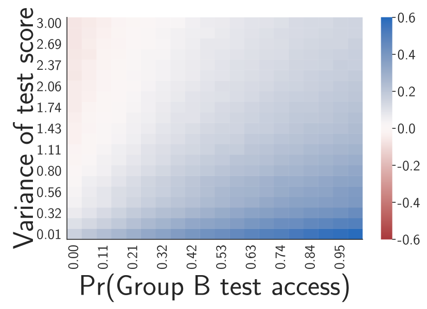
(a) Difference in Average admitted skill

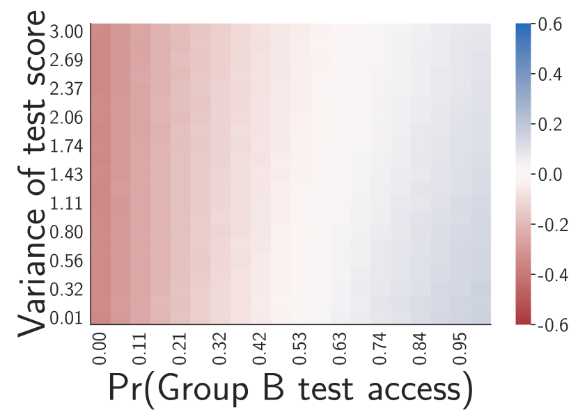
(b) Difference in Diversity level

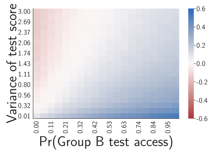
(c) Difference in Average admitted skill, Group A

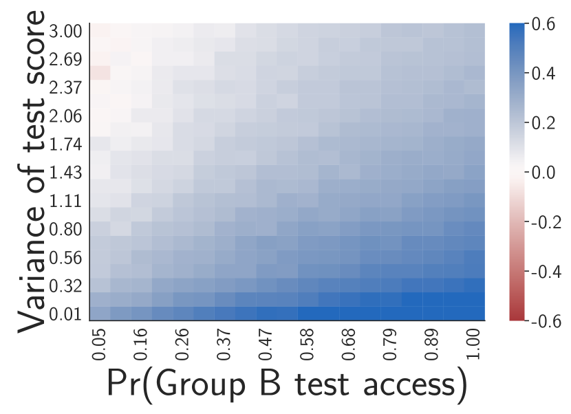
(d) Difference in Average admitted skill, Group B

Figure 9: Difference between test-based and test-free policies with respect to various objective functions. The more negative (red) the difference, the more that dropping the test improves that metric compared to test-based policies. Simulation is with budgets case, using parameters as given in Online Appendix A.3. The plot reads as follows: in Figure 9(a), a difference of $0.6$ means that the average academic merit with a test-based policy is $0.6$ higher than that with a test-free policy.

Figure 9 supplements the results in Theorem 1 and Proposition (ii), regarding the thresholds at which academic merit and diversity improve after dropping the test. In particular, they illustrate that for high enough test score variance or high enough barriers, dropping the test score improves the objectives.

A.3 Simulation parameters

Figure 2. $C=0.2,\pi=0.5,q,\theta_{A0},\theta_{A1}\sim N(0,1),\theta_{B0}\sim N(-4,5),\theta_{B1}\sim N(-4,1),\gamma_{A}=1,\gamma_{B}=\frac{2}{3}.$

Figure 3. Same as Figure 2, except with $\theta_{B1}\sim N(-4,\sigma_{B1}^{2})$, where $\sigma_{B1}^{2}\in(0,5)$. For subfigures (3(a)) - (3(c)) we fix test access $\gamma_{A}=\gamma_{B}=1$. For subfigures (3(d)) - (3(f)) fix the test score variance of group B to be equal to that of group A, so that $\sigma^{2}_{B1}=\sigma^{2}_{A1}=1$ and we vary $\gamma_{B}$.

Figure 4. Same as Figure 2.

Figure 9. Same as Figure 2, except with test score precision varying together for both groups $\sigma_{A1}^{2}=\sigma_{B1}^{2}\in(0,3)$, and group $B$ test access varying, $\gamma_{B}\in(0,1)$.

Appendix B Additional simulations for the strategic setting

B.1 Calibrated simulations with UT Austin data

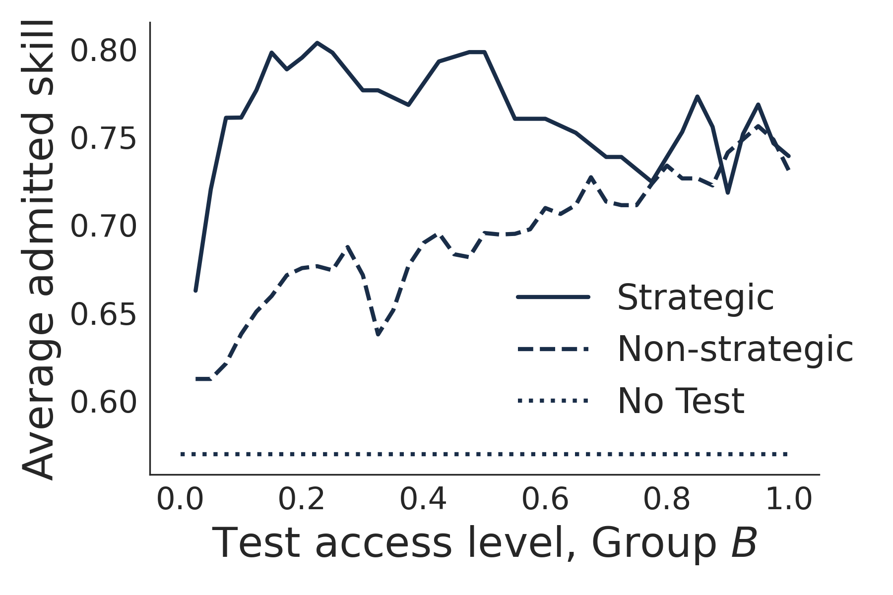
(a) Academic merit

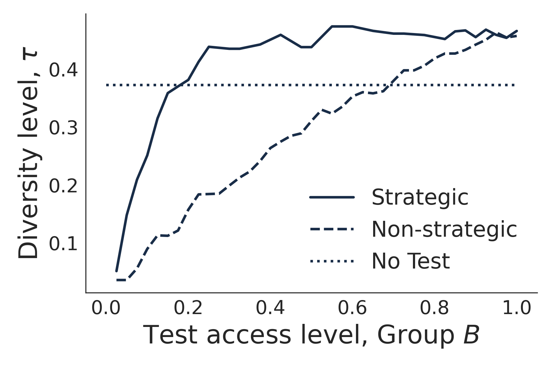
(b) Diversity level

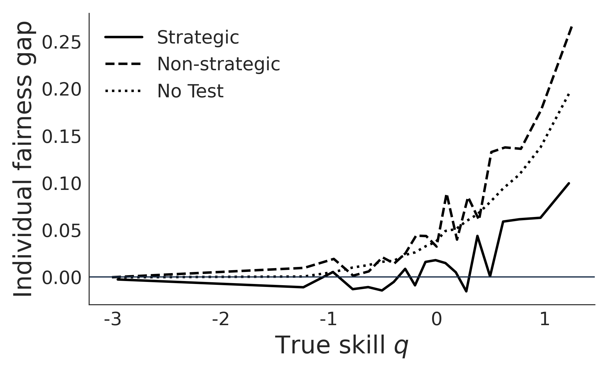
(c) Individual fairness gap

Figure 10: Calibrated simulations when full set of features is $\{$High school class rank, test score$\}$. Low informativeness case. See Table 1 for informativeness of features.

		Academic merit		Diversity Level
Informational Case	Student behavior	With test	Without test	With test	Without test
Low	Strategic	3.719	3.535	46.4%	37.1%
		$\pm$.0009	$\pm$.0009	$\pm$ .03%	$\pm$ .05%
	Non-strategic	3.643	3.535	26.6%	37.1%
		$\pm$.0008	$\pm$ .0009	$\pm$ .03%	$\pm$ .05%
High	Strategic	3.884	3.807	49.5%	48.2%
		$\pm$ .0007	$\pm$ .0008	$\pm$ 0.05%	$\pm$ 0.04%
	Non-strategic	3.788	3.807	28.4%	48.2%
		$\pm$ .0007	$\pm$ .0008	$\pm$ 0.03%	$\pm$ 0.04%

Table 3: How academic merit and diversity level of admitted students change with and without requiring a test score, for two informational cases (how informative the non-test feature is) and for the strategic and non-strategic settings. Diversity level is shown as a percentage of admitted students. Shown with 95% confidence intervals. This table assumes a 40% test access for group $B$; for outcomes for the full range of group $B$ test access, see Figures 8 and 10.

B.2 Simulations with synthetic data

We run simulations for a setting with two features, where the non-test feature is equally informative for both groups, but the test score is more informative for group $A$ than group $B$. Students have utility $v=5$ for the school, group $A$ students have test cost $c_{A}=0.5$ and we vary the test cost $c_{B}$ of group B. The school has capacity $C=0.10$.

Under these parameters, Figure 5 shows the probability of a student in group $B$ taking the test and applying, conditional on their true skill level. Figure 11 shows the application probability, academic merit, and diversity for the admission outcomes at different test costs for group $B$. Figure 6 compares the outcomes at different levels of cost and test informativeness. Figure 12 compares the admission outcomes if a school requires the test versus when it does not.

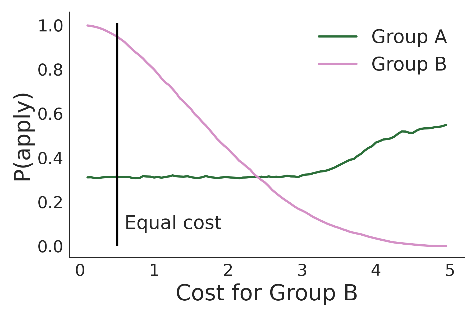
(a) Probability of applying

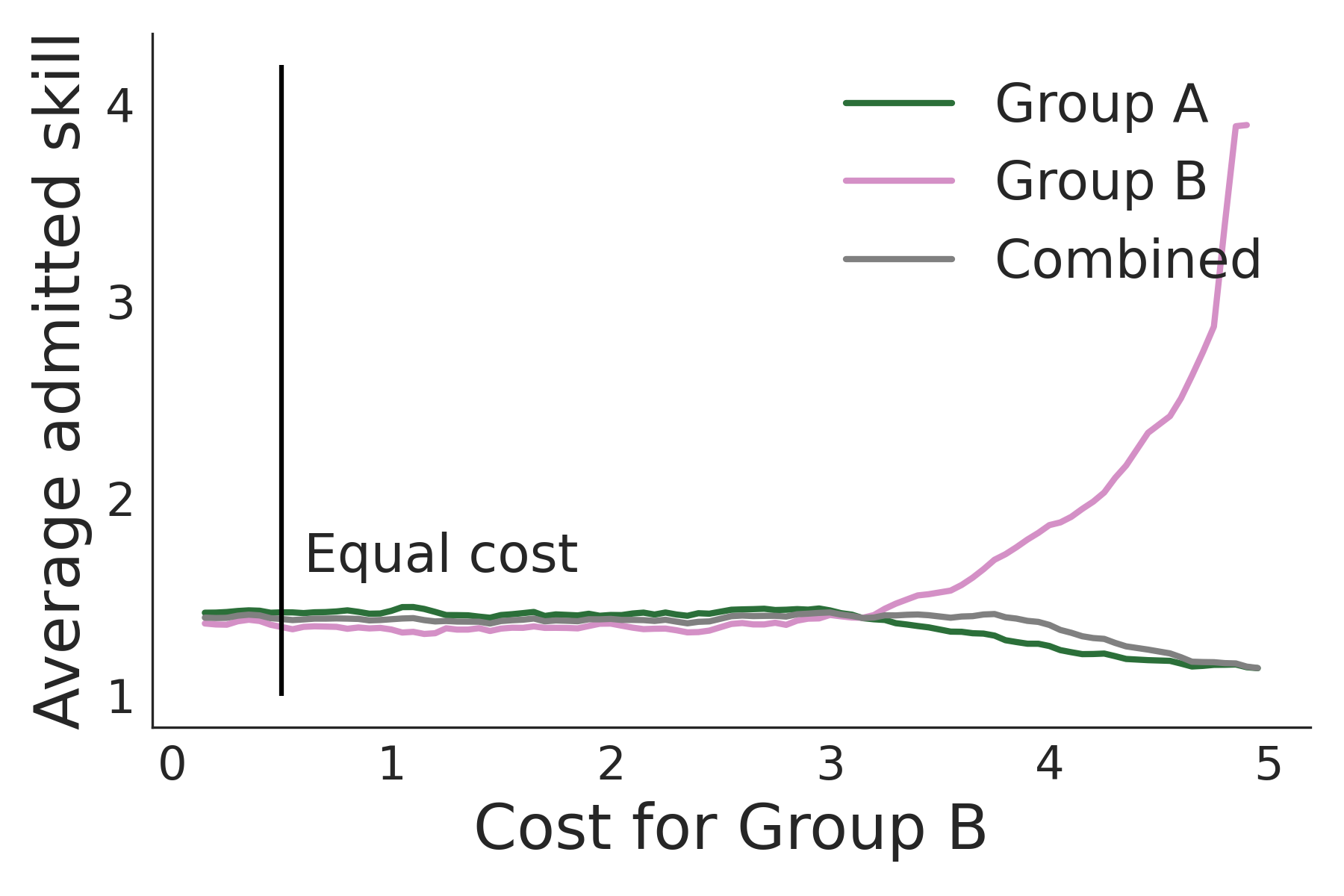
(b) Academic merit

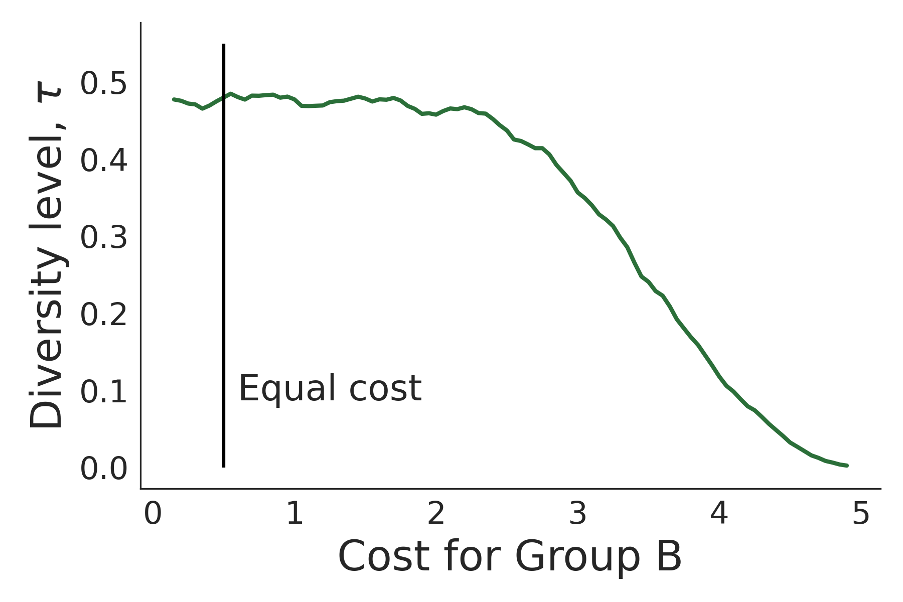
(c) Diversity level

Figure 11: Strategic students setting. How the probability of applying and the admitted students’ academic merit change when Group $A$ has cost $c_{A}=0.5$ and the cost for Group $B$ varies. As the cost for Group $B$ increases, fewer Group $B$ students apply and more Group $A$ students apply (since the threshold decreases). Academic merit of admitted Group $B$ students increases while that of Group $A$ decreases. We consider a setting where the variances of non-test features are equal for both groups, but Group $B$ has higher variance for test; the full parameter set can be found in Online Appendix B.2.

Dropping the test score. Figure 12 shows the change in the diversity level and average skill level of the admitted students, after dropping the test. In this scenario, since the variance of the non-test feature $\sigma^{2}_{A0}=\sigma^{2}_{B0}=1$ are equal for both groups, a test-free policy will have a diversity level of $\tau=0.5$.

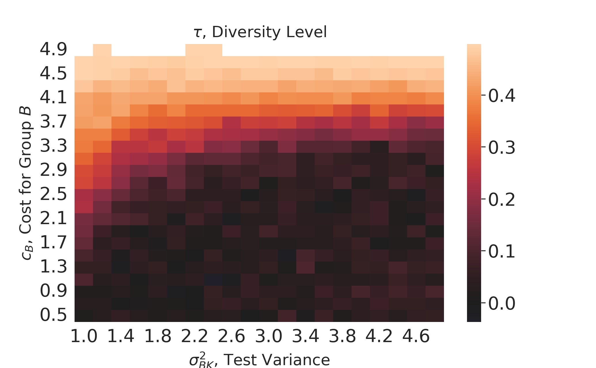
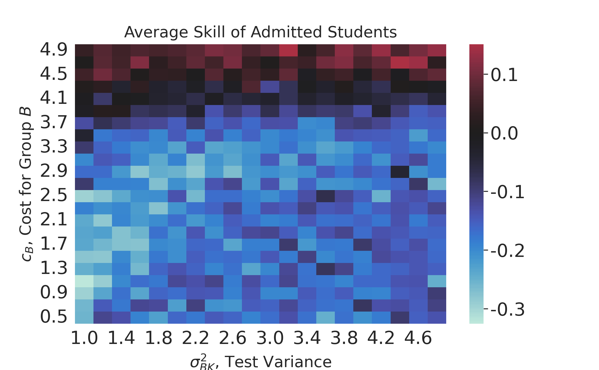
Figure 12: Change in diversity and average skill when the school drops the test requirement. When the test cost is large enough for Group $B$, dropping the test requirement increases the average academic merit and the diversity of the admitted student body. The full parameter set can be found in Online Appendix B.2.

Appendix C Proofs of statements

In this appendix, we provide and prove the full statement of each result appearing in the main text.

C.1 Auxiliary lemmas

Let $\Phi$ denote the CDF of $\mathcal{N}(0,1)$ and $\mathrm{HR}(x)=\frac{\phi(x)}{1-\Phi(x)}$ the Hazard Rate of $X\sim\mathcal{N}(0,1)$.

Lemma 1.

Let $X\mid M\sim\mathcal{N}(M,\sigma^{2})$ and $M\sim\mathcal{N}(\mu_{0},\sigma_{0}^{2})$. Then, $X\sim\mathcal{N}(\mu_{0},\sigma^{2}+\sigma^{2}_{0})$.

Lemma 2.

Let $X\mid M\sim\mathcal{N}(M,\sigma^{2})$ and $M\sim\mathcal{N}(\mu_{0},\sigma_{0}^{2})$. Then,

$$M\mid X\sim\mathcal{N}\left(\frac{\sigma_{0}^{2}}{\sigma^{2}+\sigma_{0}^{2}}X+\frac{\sigma^{2}}{\sigma^{2}+\sigma_{0}^{2}}\mu_{0},\frac{1}{\sigma^{-2}+\sigma_{0}^{-2}}\right).$$

Lemma 3.

Let $X\sim\mathcal{N}(\mu,\sigma^{2})$. Then, for any $a\in\mathbb{R}$, $\operatorname{\mathbb{E}}[X\mid X>a]=\mu+\sigma\frac{\phi(t)}{1-\Phi(t)},$ where $t=\frac{a-\mu}{\sigma}$.

Lemma 4.

The hazard rate $\mathrm{HR}(x)=\frac{\phi(x)}{1-\Phi(x)}$, $x\in\mathbb{R}$ has the following properties:

• Its derivative equals $\frac{\mathop{}\!\mathrm{d}\mathrm{HR}(x)}{\mathop{}\!\mathrm{d}x}=\mathrm{HR}(x)(\mathrm{HR}(x)-x)$;

• It holds that $\mathrm{HR}(x)>x$ for all $x>0$;

Lemma 5.

Let $a>0$. The function $h(x)=\frac{x}{a}\mathrm{HR}(\frac{a}{x})$ is increasing in $x>0$.

Proof.

Proof. Let $y=a/x$. We study the monotonicity of $\hat{h}(y)=\mathrm{HR}(y)/y$. The derivative of $\hat{h}(y)$ equals

$$\frac{\mathop{}\!\mathrm{d}\hat{h}(y)}{\mathop{}\!\mathrm{d}y}=\frac{\frac{\mathop{}\!\mathrm{d}\mathrm{HR}(y)}{\mathop{}\!\mathrm{d}y}y-\mathrm{HR}(y)}{y^{2}}.$$

For any $y>0$, it holds that $\frac{\mathop{}\!\mathrm{d}\hat{h}(y)}{\mathop{}\!\mathrm{d}y}<0$ if and only if $\frac{\mathop{}\!\mathrm{d}\mathrm{HR}(y)}{\mathop{}\!\mathrm{d}y}y-\mathrm{HR}(y)<0.$ Using Part (i) in Lemma 4, we get that

$$\frac{\mathop{}\!\mathrm{d}\mathrm{HR}(y)}{\mathop{}\!\mathrm{d}y}y-\mathrm{HR}(y)=\mathrm{HR}(y)\left(\mathrm{HR}(y)\,y-y^{2}-1\right),$$

which is negative for $y>0$ if and only if $\mathrm{HR}(y)\,y-y^{2}-1<0$ for all $y>0$.

By Theorem 2.3 in (Baricz, 2008), we know that $\mathrm{HR}(y)<\frac{y}{2}+\frac{\sqrt{y^{2}+4}}{2}.$ Thus, using this inequality, we can bound the quantity $\mathrm{HR}(y)\,y-y^{2}-1$ as follows:

$$\mathrm{HR}(y)\,y-y^{2}-1<\frac{y^{2}}{2}+y\,\frac{\sqrt{y^{2}+4}}{2}-y^{2}-1=\frac{y}{2}(-y+\sqrt{y^{2}+4})-1,$$

which is negative for any $y\in\mathbb{R}$. Therefore, $\frac{\mathop{}\!\mathrm{d}\hat{h}(y)}{\mathop{}\!\mathrm{d}y}<0$ for all $y>0$. Finally, since $\hat{h}(y)$ is decreasing in $y>0$ and $y=\frac{a}{x}$, $a>0$, is decreasing in $x>0$, it follows that $h(x)=\hat{h}\left(\frac{a}{x}\right)$ is increasing in $x>0$. ∎

C.2 Group-aware estimation

Gaussian social learning with feature set $S\subseteq\{1,\ldots,K\}$. Given that $q\sim\operatorname{\mathcal{N}}(\mu,\sigma^{2})$, $\epsilon_{kg}\sim\operatorname{\mathcal{N}}(\mu_{gk},\sigma_{gk}^{2})$ and the noise is drawn independently, each feature $k\in S$ is also normally distributed conditional on $q$, i.e., $\theta_{k}\mid q,g\sim\operatorname{\mathcal{N}}(q+\mu_{gk},\sigma_{gk}^{2}).$ Then, we inductively find that $q\mid\operatorname{\bm{\theta}},g\sim\operatorname{\mathcal{N}}\left(\tilde{q}(\operatorname{\bm{\theta}},g),\tilde{\sigma}^{2}(\operatorname{\bm{\theta}},g)\right),$ where

$$\tilde{q}(\operatorname{\bm{\theta}},g)=\frac{\mu\sigma^{-2}+\sum_{k\in S}(\theta_{k}-\mu_{gk})\sigma_{gk}^{-2}}{\sigma^{-2}+\sum_{k\in S}\sigma_{gk}^{-2}},\,\,\,\,\tilde{\sigma}^{2}(\operatorname{\bm{\theta}},g)=\frac{1}{\sigma^{-2}+\sum_{k\in S}\sigma_{gk}^{-2}}.$$ (12)

Perceived skill conditional on true skill. Equation 12 gives us the skill estimate $\tilde{q}$ of a student conditional on features $\operatorname{\bm{\theta}}$. Another useful distribution is $\tilde{q}\mid q,g,P_{S}$, which is also Gaussian. Indeed, observe that $\tilde{q}(\operatorname{\bm{\theta}},g)$ in Equation 12 is a linear combination of independent (conditional on $q$) Gaussian variables $\theta_{k}=q+\epsilon_{kg}$, $k\in S$. Thus,

$$\tilde{q}\mid q,g,P_{S}\sim\operatorname{\mathcal{N}}\left(\frac{\mu\sigma^{-2}+q\sum_{k\in S}\sigma_{gk}^{-2}}{\sigma^{-2}+\sum_{k\in S}\sigma^{-2}_{gk}},\frac{\sum_{k\in S}\sigma^{-2}_{gk}}{\left(\sigma^{-2}+\sum_{k\in S}\sigma^{-2}_{gk}\right)^{2}}\right).$$ (13)

Lemma 6.

For group-aware estimation policies, the following properties hold:

• $\operatorname{\mathbb{E}}[\tilde{q}\mid q,A,P_{S}]>\operatorname{\mathbb{E}}[\tilde{q}\mid q,B,P_{S}]$ if and only if $(q-\mu)\left(\sum_{k\in S}\sigma_{Ak}^{-2}-\sum_{k\in S}\sigma_{Bk}^{-2}\right)>0.$

• $\textrm{Var}[\tilde{q}\mid q,A,P_{S}]>\textrm{Var}[\tilde{q}\mid q,B,P_{S}]$ if and only if

  $${\left(\sigma^{-4}-\sum_{k\in S}\sigma_{Ak}^{-2}\sum_{k\in S}\sigma_{Bk}^{-2}\right)\left(\sum_{k\in S}\sigma_{Ak}^{-2}-\sum_{k\in S}\sigma_{Bk}^{-2}\right)>0.}$$

Proof.

Proof. The proof follows immediately from simple algebra thus it is ommitted. ∎

Distribution of skill estimates per group. We find the distribution $\tilde{q}\mid g,P_{S}$, that we denote by $F_{\tilde{q}\mid g,P_{S}}$.

Lemma 7 (Lemma 1).

Consider a school that uses feature set $S\subseteq\{1,\dots,K\}$ for each applicant. For $g\in\{A,B\}$, the skill level estimates for students in group $g$ are Normally distributed:

$${\tilde{q}\mid g,P_{S}}\sim\mathcal{N}\left(\mu,\sigma^{2}\left[\frac{\sum_{{k\in S}}\sigma_{gk}^{-2}}{\sigma^{-2}+\sum_{{k\in S}}\sigma_{gk}^{-2}}\right]\right).$$

Proof.

Proof. An application of Lemma 1 for $X=\tilde{q}$ and $M=\frac{\mu\sigma^{-2}+q\sum_{k\in\operatorname{\textsc{full}}}\sigma_{gk}^{-2}}{\sigma^{-2}+\sum_{k\in\operatorname{\textsc{full}}}\sigma_{gk}^{-2}}$ gives us the result. Analytically, the parameters of this distribution can be computed as follows:

$$\begin{split}\operatorname{\mathbb{E}}[\tilde{q}\mid g,P_{S}]=&\operatorname{\mathbb{E}}_{q}[\operatorname{\mathbb{E}}[\tilde{q}\mid q,g,P_{S}]]=\frac{\mu\sigma^{-2}+\mu\sum_{k\in S}\sigma_{gk}^{-2}}{\sigma^{-2}+\sum_{k\in S}\sigma_{gk}^{-2}}=\mu,\\ \textrm{Var}[\tilde{q}\mid g,P_{S}]=&\operatorname{\mathbb{E}}[\tilde{q}^{2}\mid g,P_{S}]-\mu^{2}=\operatorname{\mathbb{E}}_{q}[\operatorname{\mathbb{E}}[\tilde{q}^{2}\mid q,g,P_{S}]]-\mu^{2}\\ =&\operatorname{\mathbb{E}}_{q}\left[\textrm{Var}[\tilde{q}\mid q,g,P_{S}]+\left(\frac{\mu\sigma^{-2}+q\sum_{k\in S}\sigma_{gk}^{-2}}{\sigma^{-2}+\sum_{k\in S}\sigma_{gk}^{-2}}\right)^{2}\right]-\mu^{2}\\ =&\operatorname{\mathbb{E}}_{q}\left[\textrm{Var}[\tilde{q}\mid q,g,P_{S}]\right]+\textrm{Var}\left[\frac{\mu\sigma^{-2}+q\sum_{k\in S}\sigma_{gk}^{-2}}{\sigma^{-2}+\sum_{k\in S}\sigma_{gk}^{-2}}\right]\\ =&\frac{\sum_{k\in S}\sigma_{gk}^{-2}}{(\sigma^{-2}+\sum_{k\in S}\sigma_{gk}^{-2})^{2}}+\sigma^{2}\left(\frac{\sum_{k\in S}\sigma_{gk}^{-2}}{\sigma^{-2}+\sum_{k\in S}\sigma_{gk}^{-2}}\right)^{2}\\ =&\sigma^{2}\frac{\sum_{k\in S}\sigma_{gk}^{-2}}{\sigma^{-2}+\sum_{k\in S}\sigma_{gk}^{-2}}.\end{split}$$

∎

Corollary 1.

$\textrm{Var}[\tilde{q}\mid A,P_{S}]>\textrm{Var}[\tilde{q}\mid B,P_{S}]$ if and only if $\sum_{k\in S}\sigma_{Ak}^{-2}>\sum_{k\in S}\sigma_{Bk}^{-2}$.

Corollary 2 (Second-order stochastic dominance).

If $\sum_{k\in S}\sigma_{Ak}^{-2}>\sum_{k\in S}\sigma_{Bk}^{-2}$, then $(\tilde{q}\mid B,P_{S})\succ_{\textrm{SSD}}(\tilde{q}\mid A,P_{S})$ and $\tilde{q}\mid A,P_{S}$ is a mean-preserving spread of $\tilde{q}\mid B,P_{S}$.

Distribution of true skill conditional on skill estimate. To answer questions about the academic merit of the admitted student body, we need to be able to compute the expected value of $q$ conditional on acceptance and the social group $g$ of a student, i.e., $\operatorname{\mathbb{E}}[q\mid Y=1,g,P_{S}]$. Thus, we first the conditional distribution $q\mid\tilde{q},g,P_{S}$ in the following lemma.

Lemma 8.

Suppose that the school uses policy $P_{S}$. Then, the true skill level $q$ of students in group $g\in\{A,B\}$ conditional on the estimated skill level $\tilde{q}$ is Normally distributed as follows

$$q\mid\tilde{q},g,P_{S}\sim\operatorname{\mathcal{N}}\left(\tilde{q},\frac{1}{\sigma^{-2}+\sum_{k\in S}\sigma_{gk}^{-2}}\right).$$ (14)

Proof.

Proof. We apply Lemma 2 by using the transformation $M=\frac{\mu\sigma^{-2}+q\sum_{k\in S}\sigma_{gk}^{-2}}{\sigma^{-2}+\sum_{k\in S}\sigma_{k}\sigma_{gk}^{-2}}$ and $X=\tilde{q}$. More specifically, let

$$X\mid M\sim\operatorname{\mathcal{N}}\left(M,\frac{\sum_{k\in S}\sigma_{gk}^{-2}}{(\sigma^{-2}+\sum_{k\in S}\sigma_{gk}^{-2})^{2}}\right),\,\,\,\,M\sim\mathcal{N}\left(\mu,\sigma^{2}\left(\frac{\sum_{k\in S}\sigma_{gk}^{-2}}{\sigma^{-2}+\sum_{k\in S}\sigma_{gk}^{-2}}\right)^{2}\right).$$

Then, by Lemma 2, we get that

$$\begin{split}\operatorname{\mathbb{E}}[M\mid\tilde{q},g,P_{S}]&=\frac{\sigma^{2}\frac{(\sum_{k\in S}\sigma_{gk}^{-2})^{2}}{(\sigma^{-2}+\sum_{k\in S}\sigma_{gk}^{-2})^{2}}\tilde{q}+\mu\frac{\sum_{k\in S}\sigma_{gk}^{-2}}{(\sigma^{-2}+\sum_{k\in S}\sigma_{gk}^{-2})^{2}}}{\sigma^{2}\frac{(\sum_{k\in S}\sigma_{gk}^{-2})^{2}}{(\sigma^{-2}+\sum_{k\in S}\sigma_{gk}^{-2})^{2}}+\frac{\sum_{k\in S}\sigma_{gk}^{-2}}{(\sigma^{-2}+\sum_{k\in S}\sigma_{gk}^{-2})^{2}}}\\ &=\frac{\sum_{k\in S}\sigma_{gk}^{-2}\tilde{q}+\mu\sigma^{-2}}{\sum_{k\in S}\sigma_{gk}^{-2}+\sigma^{-2}}\\ \textrm{Var}[M\mid\tilde{q},g,P_{S}]&=\left(\left(\frac{\sum_{k\in S}\sigma_{gk}^{-2}}{(\sigma^{-2}+\sum_{k\in S}\sigma_{gk}^{-2})^{2}}\right)^{-1}+\sigma^{-2}\left(\frac{\sum_{k\in S}\sigma_{gk}^{-2}}{\sigma^{-2}+\sum_{k\in S}\sigma_{gk}^{-2}}\right)^{-2}\right)^{-1}\\ &=\frac{\left(\sum_{k\in S}\sigma_{gk}^{-2}\right)^{2}}{\left(\sigma^{-2}+\sum_{k\in S}\sigma_{gk}^{-2}\right)^{3}}.\end{split}$$

Therefore, $M\mid\tilde{q},g,P_{S}\sim\operatorname{\mathcal{N}}\left(\frac{\sum_{k\in S}\sigma_{gk}^{-2}\tilde{q}+\mu\sigma^{-2}}{\sum_{k\in S}\sigma_{gk}^{-2}+\sigma^{-2}},\frac{\left(\sum_{k\in S}\sigma_{gk}^{-2}\right)^{2}}{\left(\sigma^{-2}+\sum_{k\in S}\sigma_{gk}^{-2}\right)^{3}}\right).$ Finally, using the linear transformation

$$q=\frac{M\left(\sigma^{-2}+\sum_{k\in S}\sigma_{gk}^{-2}\right)-\mu\sigma^{-2}}{\sum_{k\in S}\sigma_{gk}^{-2}},$$

we get that $q\mid\tilde{q},g,P_{S}\sim\operatorname{\mathcal{N}}\left(\tilde{q},\frac{1}{\sigma^{-2}+\sum_{k\in S}\sigma_{gk}^{-2}}\right).$ ∎

C.3 Baseline policy in the absence of barriers

Let $\tilde{q}^{*}_{S}$ denote the optimal decision threshold used by the school under policy $P_{S}$. Using the distribution $F_{\tilde{q}\mid g,P_{S}}$, it follows that threshold $\tilde{q}^{*}_{S}$ is the solution to the equation

$$(1-\pi)F_{\tilde{q}\mid A,P_{S}}(\tilde{q}^{*}_{S})+\pi F_{\tilde{q}\mid B,P_{S}}(\tilde{q}^{*}_{S})=1-C.$$ (15)

By Lemma 1, the Gaussian mixture of $F_{\tilde{q}\mid A,P_{S}}$, $F_{\tilde{q}\mid B,P_{S}}$ with weights $1-\pi$, $\pi$ has mean $\mu$ and variance

$$(1-\pi)\sigma^{2}\left[\frac{\sum_{k\in S}\sigma_{Ak}^{-2}}{\sigma^{-2}+\sum_{k\in S}\sigma_{Ak}^{-2}}\right]+\pi\sigma^{2}\left[\frac{\sum_{k\in S}\sigma_{Bk}^{-2}}{\sigma^{-2}+\sum_{k\in S}\sigma_{Bk}^{-2}}\right].$$

Recall that for a Gaussian random variable $X\sim N(\mu_{0},\sigma_{0}^{2})$, it holds that $\frac{X-\mu_{0}}{\sigma_{0}}\sim N(0,1)$. Thus, Equation 15 can be equivalently written as

$$\Phi\left(\left(\tilde{q}^{*}_{S}-\mu\right)\left((1-\pi)\sigma^{2}\left[\frac{\sum_{k\in S}\sigma_{Ak}^{-2}}{\sigma^{-2}+\sum_{k\in S}\sigma_{Ak}^{-2}}\right]+\pi\sigma^{2}\left[\frac{\sum_{k\in S}\sigma_{Bk}^{-2}}{\sigma^{-2}+\sum_{k\in S}\sigma_{Bk}^{-2}}\right]\right)^{-1/2}\right)=1-C.$$ (16)

We also introduce some additional definitions. Given any fixed value of $\sum_{k\in S}\sigma_{Bk}^{-2}$, the informativeness gap $\Delta$ is defined as $\Delta=\sum_{k\in S}\sigma_{Ak}^{-2}-\sum_{k\in S}\sigma_{Bk}^{-2}$. Given all parameters, except $\sum_{k\in S}\sigma_{Ak}^{-2}$ fixed, let $F_{\tilde{q}\mid g,P_{S}}(q;\Delta)$ denote the CDF $F_{\tilde{q}\mid g,P_{S}}$ parameterized by $\Delta\geq 0$ and $\tilde{q}^{*}_{S}(\Delta)$ and $\tau(P_{S};\Delta)$ denote the corresponding admission threshold and diversity level, respectively, for any $\Delta\geq 0$ under the baseline policy $P_{S}$.

We now provide the proof to Proposition 1. Note that the result below considers a general feature set $S$ where the assumption on unequal precisions holds.

See 1

Proof.

Proof of Part (i). We break the proof into two steps.

Step 1: We show that group fairness fails except for equal precision. Given unequal precisions, we further show that $\tau(P_{S})<\pi$. If $\sum_{k\in S}\sigma_{Ak}^{-2}=\sum_{k\in S}\sigma_{Bk}^{-2}$, then the two distributions $F_{\tilde{q}\mid A,P_{S}}$, $F_{\tilde{q}\mid B,P_{S}}$ are identical so it trivially holds that $F_{\tilde{q}\mid A,P_{S}}(\tilde{q}_{S}^{*})=F_{\tilde{q}\mid A,P_{S}}(\tilde{q}_{S}^{*})=1-C$. Consequently, group fairness is achieved.

Next, assume that $\sum_{k\in S}\sigma_{Ak}^{-2}>\sum_{k\in S}\sigma_{Bk}^{-2}$. Then, by Lemma 1 and Corollary 2, $(\tilde{q}\mid B,P_{S})\succ_{SSD}(\tilde{q}\mid A,P_{S})$ and $\tilde{q}\mid A,P_{S}$ is a mean-preserving spread of $\tilde{q}\mid B,P_{S}$. Thus, the CDFs $F_{\tilde{q}\mid A,P_{S}}$ and $F_{\tilde{q}\mid B,P_{S}}$ cross once at $\tilde{q}=\mu$. Furthermore, $F_{\tilde{q}\mid A,P_{S}}(\tilde{q})<F_{\tilde{q}\mid B,P_{S}}(\tilde{q})$, for $\tilde{q}>\mu$ and $F_{\tilde{q}\mid A,P_{S}}(\tilde{q})>F_{\tilde{q}\mid B,P_{S}}(\tilde{q})$, for $\tilde{q}<\mu$.

Since $C<0.5=F_{\tilde{q}\mid A,P_{S}}(\mu)=F_{\tilde{q}\mid B,P_{S}}(\mu)$, then $\tilde{q}_{S}^{*}>\mu$. Therefore, $F_{\tilde{q}\mid A,P_{S}}(\tilde{q}_{S}^{*})<F_{\tilde{q}\mid B,P_{S}}(\tilde{q}_{S}^{*})$, which due to Equation 15 implies that $1-F_{\tilde{q}\mid B,P_{S}}(\tilde{q}_{S}^{*})<C$ thus

$$\tau(P_{S})=\frac{\pi(1-F_{\tilde{q}\mid B,P_{S}}(\tilde{q}^{*}_{S}))}{C}<\pi.$$

Step 2: We show that the marginal effect of $\Delta$ on $\tau(P_{S})$ is negative. Consider $0\leq\Delta<\Delta^{\prime}$. Since $F_{\tilde{q}\mid B,P_{S}}(q;\Delta)$ depends only on $\sum_{k\in S}\sigma_{Bk}^{-2}$, it remains unchanged under both $\Delta,\Delta^{\prime}$.

Recall that the admission threshold is the solution to Equation 16. Solving for $\tilde{q}^{*}_{S}(\Delta)$ gives us

$$\tilde{q}^{*}_{S}(\Delta)=\mu+\Phi^{-1}(1-C)\cdot\left((1-\pi)\sigma^{2}\left[\frac{\sum_{k\in S}\sigma_{Bk}^{-2}+\Delta}{\sigma^{-2}+\sum_{k\in S}\sigma_{Bk}^{-2}+\Delta}\right]+\pi\sigma^{2}\left[\frac{\sum_{k\in S}\sigma_{Bk}^{-2}}{\sigma^{-2}+\sum_{k\in S}\sigma_{Bk}^{-2}}\right]\right)^{1/2},$$ (17)

which is an increasing function of $\Delta$. Thus, $\tilde{q}^{*}_{S}(\Delta^{\prime})>\tilde{q}^{*}_{S}(\Delta)$.

Therefore, given that the capacity remains constant at $C$, the diversity level decreases as $\Delta$ increases since

$$\begin{split}\tau(P_{S};\Delta^{\prime})=\frac{\pi(1-F_{\tilde{q}\mid B,P_{S}}(\tilde{q}^{*}_{S}(\Delta^{\prime});\Delta^{\prime}))}{C}=\frac{\pi(1-F_{\tilde{q}\mid B,P_{S}}(\tilde{q}^{*}_{S}(\Delta^{\prime});\Delta))}{C}<\frac{\pi(1-F_{\tilde{q}\mid B,P_{S}}(\tilde{q}^{*}_{S}(\Delta);\Delta))}{C}=\tau(P_{S};\Delta).\end{split}$$

∎

Proof.

Proof of Part (ii). We prove each claim in different steps.

Step 1: We show that $I(q;P_{S})>0$ if and only if

$$q>\tilde{q}^{*}_{S}+\frac{\sigma^{-2}(\tilde{q}^{*}_{S}-\mu)}{\sqrt{\sum_{k\in S}\sigma_{Bk}^{-2}}\sqrt{\sum_{k\in S}\sigma_{Ak}^{-2}}}.$$

Recall that for a Gaussian variable $X\sim N(\mu_{0},\sigma_{0}^{2})$, it holds that $\frac{X-\mu_{0}}{\sigma_{0}}\sim N(0,1)$. Thus, given policy $P_{S}$, the probability of admission for a student in group $g$ equals

$$\operatorname{\mathbb{P}}[Y=1\mid q,g,P_{S}]=1-F_{\tilde{q}\mid q,g,P_{S}}(\tilde{q}^{*}_{S})=1-\Phi\left(\frac{\sigma^{-2}+\sum_{k\in S}\sigma^{-2}_{gk}}{\sqrt{\sum_{k\in S}\sigma^{-2}_{gk}}}\left(\tilde{q}^{*}_{S}-\frac{\mu\sigma^{-2}+q\sum_{k\in S}\sigma_{gk}^{-2}}{\sigma^{-2}+\sum_{k\in S}\sigma_{gk}^{-2}}\right)\right),$$ (18)

where

$$\mathbb{E}[\tilde{q}\mid q,g,P_{S}]=\frac{\mu\sigma^{-2}+q\sum_{k\in S}\sigma_{gk}^{-2}}{\sigma^{-2}+\sum_{k\in S}\sigma_{gk}^{-2}},\textrm{Var}[\tilde{q}\mid q,g,P_{S}]=\frac{\sum_{k\in S}\sigma^{-2}_{gk}}{\left(\sigma^{-2}+\sum_{k\in S}\sigma^{-2}_{gk}\right)^{2}}.$$

Consequently, due to the monotonicity of $\Phi$, it holds that $I(q;P_{S})>0$ if and only if

$$\begin{split}&\frac{\sigma^{-2}+\sum_{k\in S}\sigma^{-2}_{Ak}}{\sqrt{\sum_{k\in S}\sigma^{-2}_{Ak}}}\left(\tilde{q}^{*}_{S}-\frac{\mu\sigma^{-2}+q\sum_{k\in S}\sigma_{Ak}^{-2}}{\sigma^{-2}+\sum_{k\in S}\sigma_{Ak}^{-2}}\right)<\frac{\sigma^{-2}+\sum_{k\in S}\sigma^{-2}_{Bk}}{\sqrt{\sum_{k\in S}\sigma^{-2}_{Bk}}}\left(\tilde{q}^{*}_{S}-\frac{\mu\sigma^{-2}+q\sum_{k\in S}\sigma_{Bk}^{-2}}{\sigma^{-2}+\sum_{k\in S}\sigma_{Bk}^{-2}}\right)\\ &\Longleftrightarrow\frac{\tilde{q}^{*}_{S}\sigma^{-2}+\tilde{q}^{*}_{S}\sum_{k\in S}\sigma_{Ak}^{-2}-\mu\sigma^{-2}-q\sum_{k\in S}\sigma_{Ak}^{-2}}{\sqrt{\sum_{k\in S}\sigma_{Ak}^{-2}}}<\frac{\tilde{q}^{*}_{S}\sigma^{-2}+\tilde{q}^{*}_{S}\sum_{k\in S}\sigma_{Bk}^{-2}-\mu\sigma^{-2}-q\sum_{k\in S}\sigma_{Bk}^{-2}}{\sqrt{\sum_{k\in S}\sigma_{Bk}^{-2}}}\\ &\Longleftrightarrow\left(\sqrt{\sum_{k\in S}\sigma_{Bk}^{-2}}-\sqrt{\sum_{k\in S}\sigma_{Ak}^{-2}}\right)\left(\sigma^{-2}(\tilde{q}^{*}_{S}-\mu)+(q-\tilde{q}^{*}_{S})\sqrt{\sum_{k\in S}\sigma_{Bk}^{-2}}\sqrt{\sum_{k\in S}\sigma_{Ak}^{-2}}\right)<0.\end{split}$$ (19)

Due to our assumption on unequal precisions, the last inequality further translates to

$$(\tilde{q}^{*}_{S}-q)\sqrt{\sum_{k\in S}\sigma_{Bk}^{-2}}\sqrt{\sum_{k\in S}\sigma_{Ak}^{-2}}<\sigma^{-2}(\tilde{q}^{*}_{S}-\mu),$$

where the RHS is always positive due to school selectivity which implies that $\tilde{q}^{*}_{S}>\mu$. Thus, we conclude that $I(q;P_{S})>0$ if and only if

$$q>\tilde{q}^{*}_{S}+\frac{\sigma^{-2}(\tilde{q}^{*}_{S}-\mu)}{\sqrt{\sum_{k\in S}\sigma_{Bk}^{-2}}\sqrt{\sum_{k\in S}\sigma_{Ak}^{-2}}}.$$

Step 2: We show that individual fairness fails except for equal precisions. As an immediate corollary of the previous analysis in Step 1, observe that individual fairness fails unless the LHS in Equation 19 equals 0 for all $q$; equivalently, individual fairness fails except for equal precision, i.e., $\sqrt{\sum_{k\in S}\sigma_{Bk}^{-2}}-\sqrt{\sum_{k\in S}\sigma_{Ak}^{-2}}=0$.

Step 3: Finally, we show that for $q>\mu+\sigma\Phi^{-1}(1-C)$, $I(q;P_{S})$ increases as the informativeness gap increases. We begin with group $B$. By Equation 13, it follows that

$$\begin{split}\operatorname{\mathbb{P}}[Y=1\mid q,B,P_{S},\Delta]=1-F_{\tilde{q}\mid B,P_{S}}(\tilde{q}^{*}_{S}(\Delta);\Delta)=1-\Phi\left(\frac{\sigma^{-2}+\sum_{k\in S}\sigma^{-2}_{Bk}}{\sqrt{\sum_{k\in S}\sigma^{-2}_{Bk}}}\left(\tilde{q}^{*}_{S}(\Delta)-\frac{\mu\sigma^{-2}+q\sum_{k\in S}\sigma_{Bk}^{-2}}{\sigma^{-2}+\sum_{k\in S}\sigma^{-2}_{Bk}}\right)\right).\end{split}$$

By Equation 17, it further follows that $\tilde{q}^{*}_{S}(\Delta)$ is increasing in $\Delta$. Consequently, the above probability is decreasing in $\Delta$ since $\Phi$ is an increasing function and all terms except for $\tilde{q}^{*}_{S}(\Delta)$ do not depend on $\Delta$. Therefore, we conclude that the admission probability of group $B$ students decreases for any $q$ as $\Delta$ increases.

Next, for group $A$, note that students with $q>\mu+\sigma\Phi^{-1}(1-C)$ are exactly those students in group $A$ who – given perfectly observable skills $q$ – would be admitted to the class; due to imperfect information, a group $A$ student of true skill $q>\mu+\sigma\Phi^{-1}(1-C)$ has a non-zero probability to get rejected. Next, observe that as $\Delta$ increases, the total precision $\sum_{k\in S}\sigma^{-2}_{Ak}$ of group $A$ must increase. Consequently, the variance $\textrm{Var}[\tilde{q}\mid q,A,P_{S}]$ decreases thus the estimates $\tilde{q}\mid q,A,P_{S}$ of all group $A$ students (including those with true skill $q>\mu+\sigma\Phi^{-1}(1-C)$) become more precise. Combining this observation with the facts that the capacity $C$ remains constant and the admission probability of group $B$ students decreases, it follows that the probability that the top-skilled group $A$ students with $q>\mu+\sigma\Phi^{-1}(1-C)$ are rejected (either in favor of lower-skilled students in $A$ or students in $B$) decreases as $\Delta$ increases. Equivalently, their admission probability $\operatorname{\mathbb{P}}[Y=1\mid q,A,P_{S},\Delta]$ increases as $\Delta$ grows.

Putting everything together, we conclude that, given $q>\mu+\sigma\Phi^{-1}(1-C)$, the individual fairness gap $I(q;P_{S})$ increases as the informativeness gap $\Delta$ increases. ∎

Proof.

Proof of Part (iii). We break the proof into the following steps.

Step 1: We compute the expected value $\operatorname{\mathbb{E}}[\tilde{q}\mid Y=1,g,P_{S}]$ and show that $\operatorname{\mathbb{E}}[\tilde{q}\mid Y=1,A,P_{S}]\geq\operatorname{\mathbb{E}}[\tilde{q}\mid Y=1,B,P_{S}]$. Applying Lemma 3, we get that

$$\begin{split}\operatorname{\mathbb{E}}[\tilde{q}\mid Y=1,g,P_{S}]=\operatorname{\mathbb{E}}[\tilde{q}\mid\tilde{q}\geq\tilde{q}_{S}^{*},g,P_{S}]&=\operatorname{\mathbb{E}}[\tilde{q}\mid g]+\sqrt{\textrm{Var}[\tilde{q}\mid g,P_{S}]}\frac{\phi(t_{g})}{1-\Phi(t_{g})}\\ &=\mu+\sigma\sqrt{\frac{\sum_{k\in S}\sigma_{gk}^{-2}}{\sigma^{-2}+\sum_{k\in S}\sigma_{gk}^{-2}}}\cdot\frac{\phi(t_{g})}{1-\Phi(t_{g})},\end{split}$$ (20)

where $t_{g}=\frac{\tilde{q}_{S}^{*}-\operatorname{\mathbb{E}}[\tilde{q}\mid g,P_{S}]}{\sqrt{\textrm{Var}[\tilde{q}\mid g,P_{S}]}}$. Due to school selectivity, we have $\tilde{q}_{S}^{*}>\mu$. By Lemma 5, the function

$$h(x)=x\frac{\phi\left(\frac{\tilde{q}^{*}_{S}-\mu}{x}\right)}{1-\Phi\left(\frac{\tilde{q}^{*}_{S}-\mu}{x}\right)}=x\textrm{HR}\left(\frac{\tilde{q}^{*}_{S}-\mu}{x}\right)$$

is increasing in $x>0$ for $\tilde{q}_{S}^{*}>\mu$. Thus, by Corollary 1, we get that that

$$\operatorname{\mathbb{E}}[\tilde{q}\mid\tilde{q}\geq\tilde{q}_{S}^{*},A,P_{S}]\geq\operatorname{\mathbb{E}}[\tilde{q}\mid\tilde{q}\geq\tilde{q}_{S}^{*},B,P_{S}].$$

Step 2: We compute the expected value $\operatorname{\mathbb{E}}[q\mid\tilde{q}\geq\tilde{q}_{K}^{*},g,P_{S}]$. Specifically,

$$\begin{split}\operatorname{\mathbb{E}}[q\mid Y=1,g,P_{S}]=\operatorname{\mathbb{E}}[q\mid\tilde{q}\geq\tilde{q}_{K}^{*},g,P_{S}]=\operatorname{\mathbb{E}}_{\tilde{q}}[\operatorname{\mathbb{E}}_{q}[q\mid\tilde{q},g,P_{S}]\mid\tilde{q}\geq\tilde{q}_{K}^{*},g,P_{S}]=\operatorname{\mathbb{E}}[\tilde{q}\mid\tilde{q}\geq\tilde{q}_{K}^{*},g,P_{S}],\end{split}$$ (21)

where the last equality follows from Lemma 8.

Step 3: We show that $\operatorname{\mathbb{E}}[q\mid Y=1,A,P_{S}]>\operatorname{\mathbb{E}}[q\mid Y=1,B,P_{S}]$. Given our assumptions on unequal precisions and school selectivity, the proof follows immediately from Steps 1 and 2. I.e., if $\sum_{k\in S}\sigma_{Ak}^{-2}>\sum_{k\in S}\sigma_{Bk}^{-2}$ and $C<0.5$, then $\operatorname{\mathbb{E}}[q\mid Y=1,A,P_{S}]>\operatorname{\mathbb{E}}[q\mid Y=1,B,P_{S}].$ ∎

Explaining why the individual fairness gap decreases for high-skilled students. Although the individual fairness gap is positive for sufficiently high-skilled students, the magnitude of this gap varies. For students at the end of the right tail of the true skill distribution, the individual fairness gap starts to decrease. This property can be graphically observed in Figure 4(b).

See 1

Proof.

Proof. By Equation 13, the individual fairness gap equals

$$I(q;P_{S})=\left(1-\Phi\left(\frac{\sigma^{-2}+\sum_{k\in S}\sigma^{-2}_{Ak}}{\sqrt{\sum_{k\in S}\sigma^{-2}_{Ak}}}\left(\tilde{q}^{*}_{S}-\frac{\mu\sigma^{-2}+q\sum_{k\in S}\sigma_{Ak}^{-2}}{\sigma^{-2}+\sum_{k\in S}\sigma^{-2}_{Ak}}\right)\right)\right)-\left(1-\Phi\left(\frac{\sigma^{-2}+\sum_{k\in S}\sigma^{-2}_{Bk}}{\sqrt{\sum_{k\in S}\sigma^{-2}_{Bk}}}\left(\tilde{q}^{*}_{S}-\frac{\mu\sigma^{-2}+q\sum_{k\in S}\sigma_{Bk}^{-2}}{\sigma^{-2}+\sum_{k\in S}\sigma^{-2}_{Bk}}\right)\right)\right).$$

Taking the derivative of $I(q;P_{S})$ with respect to $q$, we find that

$$\begin{split}\frac{\mathop{}\!\mathrm{d}I(q;P_{S})}{\mathop{}\!\mathrm{d}q}=&\phi\left(\frac{\sigma^{-2}+\sum_{k\in S}\sigma^{-2}_{Ak}}{\sqrt{\sum_{k\in S}\sigma^{-2}_{Ak}}}\left(\tilde{q}^{*}_{S}-\frac{\mu\sigma^{-2}+q\sum_{k\in S}\sigma_{Ak}^{-2}}{\sigma^{-2}+\sum_{k\in S}\sigma^{-2}_{Ak}}\right)\right)\sqrt{\sum_{k\in S}\sigma^{-2}_{Ak}}\\ &-\phi\left(\frac{\sigma^{-2}+\sum_{k\in S}\sigma^{-2}_{Bk}}{\sqrt{\sum_{k\in S}\sigma^{-2}_{Bk}}}\left(\tilde{q}^{*}_{S}-\frac{\mu\sigma^{-2}+q\sum_{k\in S}\sigma_{Bk}^{-2}}{\sigma^{-2}+\sum_{k\in S}\sigma^{-2}_{Bk}}\right)\right)\sqrt{\sum_{k\in S}\sigma^{-2}_{Bk}}.\end{split}$$

Thus, to prove that $\frac{\mathop{}\!\mathrm{d}I(q;P_{S})}{\mathop{}\!\mathrm{d}q}<0$, it suffices to show that

$$\begin{split}&\ln\left(\phi\left(\frac{\sigma^{-2}+\sum_{k\in S}\sigma^{-2}_{Ak}}{\sqrt{\sum_{k\in S}\sigma^{-2}_{Ak}}}\left(\tilde{q}^{*}_{S}-\frac{\mu\sigma^{-2}+q\sum_{k\in S}\sigma_{Ak}^{-2}}{\sigma^{-2}+\sum_{k\in S}\sigma^{-2}_{Ak}}\right)\right)\sqrt{\sum_{k\in S}\sigma^{-2}_{Ak}}\right)\\ <&\ln\left(\phi\left(\frac{\sigma^{-2}+\sum_{k\in S}\sigma^{-2}_{Bk}}{\sqrt{\sum_{k\in S}\sigma^{-2}_{Bk}}}\left(\tilde{q}^{*}_{S}-\frac{\mu\sigma^{-2}+q\sum_{k\in S}\sigma_{Bk}^{-2}}{\sigma^{-2}+\sum_{k\in S}\sigma^{-2}_{Bk}}\right)\right)\sqrt{\sum_{k\in S}\sigma^{-2}_{Bk}}\right).\end{split}$$

The above condition is equivalent to

$$\begin{split}&-\frac{\left((\tilde{q}^{*}_{S}-\mu)\sigma^{-2}+(\tilde{q}^{*}_{S}-q)\sum_{k\in S}\sigma^{-2}_{Ak}\right)^{2}}{\sum_{k\in S}\sigma^{-2}_{Ak}}+\ln\left(\sum_{k\in S}\sigma^{-2}_{Ak}\right)<-\frac{\left((\tilde{q}^{*}_{S}-\mu)\sigma^{-2}+(\tilde{q}^{*}_{S}-q)\sum_{k\in S}\sigma^{-2}_{Bk}\right)^{2}}{\sum_{k\in S}\sigma^{-2}_{Bk}}+\ln\left(\sum_{k\in S}\sigma^{-2}_{Bk}\right)\\ \Longleftrightarrow&\left({\sum_{k\in S}\sigma^{-2}_{Ak}}-{\sum_{k\in S}\sigma^{-2}_{Bk}}\right)\left(\sigma^{-4}(\mu-\tilde{q}^{*}_{S})^{2}-{\sum_{k\in S}\sigma^{-2}_{Ak}}{\sum_{k\in S}\sigma^{-2}_{Bk}}(q-\tilde{q}^{*}_{S})^{2}\right)+{\sum_{k\in S}\sigma^{-2}_{Ak}}{\sum_{k\in S}\sigma^{-2}_{Bk}}\ln\left(\frac{{\sum_{k\in S}\sigma^{-2}_{Ak}}}{{\sum_{k\in S}\sigma^{-2}_{Bk}}}\right)<0.\end{split}$$

Given our assumption on unequal precision, i.e., ${\sum_{k\in S}\sigma^{-2}_{Bk}}<{\sum_{k\in S}\sigma^{-2}_{Ak}},$ we further get that this condition is satisfied for

$$q>q_{e}\triangleq\tilde{q}^{*}_{S}+\sqrt{\frac{\sigma^{-4}(\mu-\tilde{q}^{*}_{S})^{2}}{{\sum_{k\in S}\sigma^{-2}_{Ak}}{\sum_{k\in S}\sigma^{-2}_{Bk}}}+\frac{\ln\left({{\sum_{k\in S}\sigma^{-2}_{Ak}}}\right)-\ln\left({{\sum_{k\in S}\sigma^{-2}_{Bk}}}\right)}{{\sum_{k\in S}\sigma^{-2}_{Ak}}-{\sum_{k\in S}\sigma^{-2}_{Bk}}}}.$$

Therefore, the individual fairness gap $I(q;P_{S})$ is decreasing in $q$ for $q>q_{e}$ as desired.

Furthermore, by the definition of $I(q;P_{S})$ and the fact that $\lim_{q^{\prime}\rightarrow\infty}\Phi(q^{\prime})=1$, we immediately get that $\lim_{q\rightarrow\infty}I(q;P_{S})=0.$ ∎

C.4 Dropping a feature in the absence of barriers

We are interested in comparing group-aware policies $P_{\operatorname{\textsc{full}}}$ and $P_{\operatorname{\textsc{sub}}}$. By our previous result in Lemma 1, we get that

$$\tilde{q}\mid g,P_{\operatorname{\textsc{sub}}}\sim\operatorname{\mathcal{N}}\left(\mu,\sigma^{2}\frac{\sum_{k\in\operatorname{\textsc{sub}}}\sigma_{gk}^{-2}}{\sigma^{-2}+\sum_{k\in\operatorname{\textsc{sub}}}\sigma_{gk}^{-2}}\right),\,\,\,\,\tilde{q}\mid g,P_{\operatorname{\textsc{full}}}\sim\operatorname{\mathcal{N}}\left(\mu,\sigma^{2}\frac{\sum_{k\in\operatorname{\textsc{full}}}\sigma_{gk}^{-2}}{\sigma^{-2}+\sum_{k\in\operatorname{\textsc{full}}}\sigma_{gk}^{-2}}\right).$$

Lemma 9.

The variance of $\tilde{q}\mid g,P_{\operatorname{\textsc{sub}}}$ is lower than that of $\tilde{q}\mid g,P_{\operatorname{\textsc{full}}}$ but their means are both equal to $\mu$.

Proof.

Proof. The proof follows trivially from the fact that the function $h(x)=\frac{x}{\sigma^{-2}+x}$ is increasing in $x>0$ and

$$\sum_{k\in\operatorname{\textsc{full}}}\sigma_{gk}^{-2}=\sum_{k=1}^{K}\sigma_{gk}^{-2}>\sum_{k=1}^{K-1}\sigma_{gk}^{-2}=\sum_{k\in\operatorname{\textsc{sub}}}\sigma_{gk}^{-2}$$

for any $g$. ∎

Let $\tilde{q}^{*}_{\operatorname{\textsc{sub}}}$ be the decision threshold of a school considering only features $k=1$ to $K-1$. By Equation 15, $\tilde{q}^{*}_{\operatorname{\textsc{sub}}}$ is the solution to the following equation

$$(1-\pi)F_{\tilde{q}\mid A,P_{\operatorname{\textsc{sub}}}}(\tilde{q}^{*}_{\operatorname{\textsc{sub}}})+\pi F_{\tilde{q}\mid A,P_{\operatorname{\textsc{sub}}}}(\tilde{q}^{*}_{\operatorname{\textsc{sub}}})=1-C,$$

whereas $\tilde{q}^{*}_{\operatorname{\textsc{full}}}$ is the solution to

$$(1-\pi)F_{\tilde{q}\mid A,P_{\operatorname{\textsc{full}}}}(\tilde{q}^{*}_{\operatorname{\textsc{full}}})+\pi F_{\tilde{q}\mid A,P_{\operatorname{\textsc{full}}}}(\tilde{q}^{*}_{\operatorname{\textsc{full}}})=1-C.$$

Lemma 10.

The admission threshold decreases after dropping feature $k=K$, i.e., $\tilde{q}^{*}_{\operatorname{\textsc{sub}}}<\tilde{q}^{*}_{\operatorname{\textsc{full}}}$.

Proof.

Proof. The proof follows from the definitions of $\tilde{q}^{*}_{\operatorname{\textsc{sub}}},\tilde{q}^{*}_{\operatorname{\textsc{full}}}$, and Lemma 9. ∎

See 2

Proof.

Proof of Part (i). Diversity improves if and only if

$$\tau(P_{\operatorname{\textsc{sub}}})=1-F_{\tilde{q}\mid A,P_{\operatorname{\textsc{sub}}}}(\tilde{q}^{*}_{\operatorname{\textsc{sub}}})>1-F_{\tilde{q}\mid A,P_{\operatorname{\textsc{full}}}}(\tilde{q}_{a})=\tau(P_{\operatorname{\textsc{full}}}).$$

By the definition of diversity level and Lemma 1, this is equivalent to the following condition

$$1-\Phi\left(\frac{\tilde{q}^{*}_{\operatorname{\textsc{sub}}}-\mu}{\sigma\sqrt{\frac{\sum_{k\in\operatorname{\textsc{sub}}}\sigma^{-2}_{Bk}}{\sum_{k\in\operatorname{\textsc{sub}}}\sigma^{-2}_{Bk}+\sigma^{-2}}}}\right)>1-\Phi\left(\frac{\tilde{q}^{*}_{\operatorname{\textsc{full}}}-\mu}{\sigma\sqrt{\frac{\sum_{k\in\operatorname{\textsc{full}}}\sigma^{-2}_{Bk}}{\sum_{k\in\operatorname{\textsc{full}}}\sigma^{-2}_{Bk}+\sigma^{-2}}}}\right).$$

Replacing $\tilde{q}^{*}_{\operatorname{\textsc{full}}},\tilde{q}^{*}_{\operatorname{\textsc{sub}}}$ with their definitions as in Equation 16, the above inequality becomes

$$\Phi\left(\Phi^{-1}(1-C)\sqrt{(1-\pi)\frac{\frac{\sum_{k\in\operatorname{\textsc{sub}}}\sigma_{Ak}^{-2}}{\sigma^{-2}+\sum_{k\in\operatorname{\textsc{sub}}}\sigma_{Ak}^{-2}}}{\frac{\sum_{k\in\operatorname{\textsc{sub}}}\sigma_{Bk}^{-2}}{\sigma^{-2}+\sum_{k\in\operatorname{\textsc{sub}}}\sigma_{Bk}^{-2}}}+\pi}\right)<\Phi\left(\Phi^{-1}(1-C)\sqrt{(1-\pi)\frac{\frac{\sum_{k\in\operatorname{\textsc{full}}}\sigma_{Ak}^{-2}}{\sigma^{-2}+\sum_{k\in\operatorname{\textsc{full}}}\sigma_{Ak}^{-2}}}{\frac{\sum_{k\in\operatorname{\textsc{full}}}\sigma_{Bk}^{-2}}{\sigma^{-2}+\sum_{k\in\operatorname{\textsc{full}}}\sigma_{Bk}^{-2}}}+\pi}\right),$$

which – due to the monotonicity of $\Phi$ – holds if and only if

$$\frac{\frac{\sum_{k\in\operatorname{\textsc{sub}}}\sigma_{Ak}^{-2}}{\sigma^{-2}+\sum_{k\in\operatorname{\textsc{sub}}}\sigma_{Ak}^{-2}}}{\frac{\sum_{k\in\operatorname{\textsc{sub}}}\sigma_{Bk}^{-2}}{\sigma^{-2}+\sum_{k\in\operatorname{\textsc{sub}}}\sigma_{Bk}^{-2}}}<\frac{\frac{\sum_{k\in\operatorname{\textsc{full}}}\sigma_{Ak}^{-2}}{\sigma^{-2}+\sum_{k\in\operatorname{\textsc{full}}}\sigma_{Ak}^{-2}}}{\frac{\sum_{k\in\operatorname{\textsc{full}}}\sigma_{Bk}^{-2}}{\sigma^{-2}+\sum_{k\in\operatorname{\textsc{full}}}\sigma_{Bk}^{-2}}}.$$

Using the substitution $\sum_{k\in\operatorname{\textsc{full}}}\sigma_{gk}^{-2}=\sum_{k\in\operatorname{\textsc{sub}}}\sigma_{gk}^{-2}+\sigma_{gK}$, the last relation equivalently simplifies to Equation 3. ∎

Proof.

Proof of Part (ii). We prove each claim at a separate step.

Step 1: We show that, for group $B$, $\operatorname{\mathbb{P}}(Y=1\mid q,B,P_{\operatorname{\textsc{full}}})<\operatorname{\mathbb{P}}(Y=1\mid q,B,P_{\operatorname{\textsc{sub}}})$ if and only if

$$\begin{split}q<q_{B}\triangleq\mu+&\frac{\sigma\Phi^{-1}(1-C)}{\sqrt{\sum_{k\in\operatorname{\textsc{full}}}\sigma_{Bk}^{-2}}-\sqrt{\sum_{k\in\operatorname{\textsc{sub}}}\sigma_{Bk}^{-2}}}\left(\sqrt{\sigma^{-2}+\sum_{k\in\operatorname{\textsc{full}}}\sigma_{Bk}^{-2}}\sqrt{(1-\pi)\frac{\frac{\sum_{k\in\operatorname{\textsc{full}}}\sigma_{Ak}^{-2}}{\sigma^{-2}+\sum_{k\in\operatorname{\textsc{full}}}\sigma_{Ak}^{-2}}}{\frac{\sum_{k\in\operatorname{\textsc{full}}}\sigma_{Bk}^{-2}}{\sigma^{-2}+\sum_{k\in\operatorname{\textsc{full}}}\sigma_{Bk}^{-2}}}+\pi}\right.\\ &-\left.\sqrt{\sigma^{-2}+\sum_{k\in\operatorname{\textsc{sub}}}\sigma_{Bk}^{-2}}\sqrt{(1-\pi)\frac{\frac{\sum_{k\in\operatorname{\textsc{sub}}}\sigma_{Ak}^{-2}}{\sigma^{-2}+\sum_{k\in\operatorname{\textsc{sub}}}\sigma_{Ak}^{-2}}}{\frac{\sum_{k\in\operatorname{\textsc{sub}}}\sigma_{Bk}^{-2}}{\sigma^{-2}+\sum_{k\in\operatorname{\textsc{sub}}}\sigma_{Bk}^{-2}}}+\pi}\right),\end{split}$$

Similarly, for group $A$, it holds that $\operatorname{\mathbb{P}}(Y=1\mid q,A,P_{\operatorname{\textsc{full}}})>\operatorname{\mathbb{P}}(Y=1\mid q,A,P_{\operatorname{\textsc{sub}}})$ if and only if

$$\begin{split}q<q_{A}\triangleq\mu+&\frac{\sigma\Phi^{-1}(1-C)}{\sqrt{\sum_{k\in\operatorname{\textsc{full}}}\sigma_{Ak}^{-2}}-\sqrt{\sum_{k\in\operatorname{\textsc{sub}}}\sigma_{Ak}^{-2}}}\left(\sqrt{\sigma^{-2}+\sum_{k\in\operatorname{\textsc{full}}}\sigma_{Ak}^{-2}}\sqrt{(1-\pi)+\pi\frac{\frac{\sum_{k\in\operatorname{\textsc{full}}}\sigma_{Bk}^{-2}}{\sigma^{-2}+\sum_{k\in S}\sigma_{Ak}^{-2}}}{\frac{\sum_{k\in\operatorname{\textsc{full}}}\sigma_{Ak}^{-2}}{\sigma^{-2}+\sum_{k\in\operatorname{\textsc{full}}}\sigma_{Bk}^{-2}}}}\right.\\ &-\left.\sqrt{\sigma^{-2}+\sum_{k\in\operatorname{\textsc{sub}}}\sigma_{Ak}^{-2}}\sqrt{(1-\pi)+\pi\frac{\frac{\sum_{k\in\operatorname{\textsc{sub}}}\sigma_{Bk}^{-2}}{\sigma^{-2}+\sum_{k\in\operatorname{\textsc{sub}}}\sigma_{Bk}^{-2}}}{\frac{\sum_{k\in\operatorname{\textsc{sub}}}\sigma_{Ak}^{-2}}{\sigma^{-2}+\sum_{k\in\operatorname{\textsc{sub}}}\sigma_{Ak}^{-2}}}}\right),\end{split}$$

Assume $g=B$; the proof for group $A$ is analogous. Replacing $\tilde{q}^{*}_{S}$ from Equation 16 in Equation 18, we find that for policy $P_{S}$, the admissions probability (conditional on true skill $q$ and group $g$) equals

$$\operatorname{\mathbb{P}}(Y=1\mid q,B,P_{S})=1-\Phi\left((\mu-q)\sqrt{\sum_{k\in S}\sigma_{Bk}^{-2}}+\sigma\Phi^{-1}(1-C)\sqrt{\sigma^{-2}+\sum_{k\in S}\sigma_{Bk}^{-2}}\sqrt{\frac{(1-\pi)\frac{\sum_{k\in S}\sigma_{Ak}^{-2}}{\sigma^{-2}+\sum_{k\in S}\sigma_{Bk}^{-2}}+\pi\frac{\sum_{k\in S}\sigma_{Bk}^{-2}}{\sigma^{-2}+\sum_{k\in S}\sigma_{Bk}^{-2}}}{\frac{\sum_{k\in S}\sigma_{Bk}^{-2}}{\sigma^{-2}+\sum_{k\in S}\sigma_{Bk}^{-2}}}}\right).$$

Thus, the admission probability increases after dropping test scores, if and only if

$$\begin{split}(\mu-q)&\left(\sqrt{\sum_{k\in\operatorname{\textsc{full}}}\sigma_{Bk}^{-2}}-\sqrt{\sum_{k\in\operatorname{\textsc{sub}}}\sigma_{Bk}^{-2}}\right)+\sigma\Phi^{-1}(1-C)\sqrt{\sigma^{-2}+\sum_{k\in\operatorname{\textsc{full}}}\sigma_{Bk}^{-2}}\sqrt{(1-\pi)\frac{\frac{\sum_{k\in\operatorname{\textsc{full}}}\sigma_{Ak}^{-2}}{\sigma^{-2}+\sum_{k\in\operatorname{\textsc{full}}}\sigma_{Ak}^{-2}}}{\frac{\sum_{k\in\operatorname{\textsc{full}}}\sigma_{Bk}^{-2}}{\sigma^{-2}+\sum_{k\in\operatorname{\textsc{full}}}\sigma_{Bk}^{-2}}}+\pi}\\ &-\sigma\Phi^{-1}(1-C)\sqrt{\sigma^{-2}+\sum_{k\in\operatorname{\textsc{sub}}}\sigma_{Bk}^{-2}}\sqrt{(1-\pi)\frac{\frac{\sum_{k\in\operatorname{\textsc{sub}}}\sigma_{Ak}^{-2}}{\sigma^{-2}+\sum_{k\in\operatorname{\textsc{sub}}}\sigma_{Ak}^{-2}}}{\frac{\sum_{k\in\operatorname{\textsc{sub}}}\sigma_{Bk}^{-2}}{\sigma^{-2}+\sum_{k\in\operatorname{\textsc{sub}}}\sigma_{Bk}^{-2}}}+\pi}>0.\end{split}$$ (22)

This is equivalent to $q<q_{B}$, i.e.,

$$\begin{split}q<\mu+&\frac{\sigma\Phi^{-1}(1-C)}{\sqrt{\sum_{k\in\operatorname{\textsc{full}}}\sigma_{Bk}^{-2}}-\sqrt{\sum_{k\in\operatorname{\textsc{sub}}}\sigma_{Bk}^{-2}}}\left(\sqrt{\sigma^{-2}+\sum_{k\in\operatorname{\textsc{full}}}\sigma_{Bk}^{-2}}\sqrt{(1-\pi)\frac{\frac{\sum_{k\in\operatorname{\textsc{full}}}\sigma_{Ak}^{-2}}{\sigma^{-2}+\sum_{k\in\operatorname{\textsc{full}}}\sigma_{Ak}^{-2}}}{\frac{\sum_{k\in\operatorname{\textsc{full}}}\sigma_{Bk}^{-2}}{\sigma^{-2}+\sum_{k\in\operatorname{\textsc{full}}}\sigma_{Bk}^{-2}}}+\pi}\right.\\ &-\left.\sqrt{\sigma^{-2}+\sum_{k\in\operatorname{\textsc{sub}}}\sigma_{Bk}^{-2}}\sqrt{(1-\pi)\frac{\frac{\sum_{k\in\operatorname{\textsc{sub}}}\sigma_{Ak}^{-2}}{\sigma^{-2}+\sum_{k\in\operatorname{\textsc{sub}}}\sigma_{Ak}^{-2}}}{\frac{\sum_{k\in\operatorname{\textsc{sub}}}\sigma_{Bk}^{-2}}{\sigma^{-2}+\sum_{k\in\operatorname{\textsc{sub}}}\sigma_{Bk}^{-2}}}+\pi}\right),\end{split}$$

Step 2: We show that there exists a threshold $\hat{q}\geq\max\{q_{A},q_{B}\}$ such that the individual fairness gap increases for all $q>\hat{q}$. Otherwise, it may decrease. Let

$$\underline{q}\triangleq\arg\min_{q\in\mathbb{R}}\left\{(\mu-q)\sqrt{\sum_{k\in S}\sigma_{gk}^{-2}}+\sigma\Phi^{-1}(1-C)\sqrt{\sigma^{-2}+\sum_{k\in S}\sigma_{gk}^{-2}}\sqrt{\frac{(1-\pi)\frac{\sum_{k\in S}\sigma_{Ak}^{-2}}{\sigma^{-2}+\sum_{k\in S}\sigma_{Ak}^{-2}}+\pi\frac{\sum_{k\in S}\sigma_{Bk}^{-2}}{\sigma^{-2}+\sum_{k\in S}\sigma_{Bk}^{-2}}}{\frac{\sum_{k\in S}\sigma_{gk}^{-2}}{\sigma^{-2}+\sum_{k\in S}\sigma_{gk}^{-2}}}}\leq 0,\forall g,S\right\}.$$

Next, consider only $q>\max\{\underline{q},q_{A},q_{B}\}.$ Since $\Phi$ is monotone and convex in $(-\infty,0]$ and $q>\hat{q}$, and by Step 1 for any group $g$, it also holds that $\operatorname{\mathbb{P}}(Y=1\mid q,g,P_{\operatorname{\textsc{full}}})>\operatorname{\mathbb{P}}(Y=1\mid q,g,P_{\operatorname{\textsc{sub}}})$ for all $q>q_{g}$, a sufficient condition for $I(q;P_{\operatorname{\textsc{full}}})>I(q;P_{\operatorname{\textsc{sub}}})$, to hold is

$$\begin{split}&\frac{\sigma^{-2}+\sum_{k\in\operatorname{\textsc{sub}}}\sigma^{-2}_{Ak}}{\sqrt{\sum_{k\in\operatorname{\textsc{sub}}}\sigma^{-2}_{Ak}}}\left(\tilde{q}^{*}_{\operatorname{\textsc{sub}}}-\frac{\mu\sigma^{-2}+q\sum_{k\in\operatorname{\textsc{sub}}}\sigma^{-2}_{Ak}}{\sigma^{-2}+\sum_{k\in\operatorname{\textsc{sub}}}\sigma^{-2}_{Ak}}\right)-\frac{\sigma^{-2}+\sum_{k\in\operatorname{\textsc{full}}}\sigma^{-2}_{Ak}}{\sqrt{\sum_{k\in\operatorname{\textsc{full}}}\sigma^{-2}_{Ak}}}\left(\tilde{q}^{*}_{\operatorname{\textsc{full}}}-\frac{\mu\sigma^{-2}+q\sum_{k\in\operatorname{\textsc{full}}}\sigma^{-2}_{Ak}}{\sigma^{-2}+\sum_{k\in\operatorname{\textsc{full}}}\sigma^{-2}_{Ak}}\right)\\ <&\frac{\sigma^{-2}+\sum_{k\in\operatorname{\textsc{sub}}}\sigma^{-2}_{Bk}}{\sqrt{\sum_{k\in\operatorname{\textsc{sub}}}\sigma^{-2}_{Bk}}}\left(\tilde{q}^{*}_{\operatorname{\textsc{sub}}}-\frac{\mu\sigma^{-2}+q\sum_{k\in\operatorname{\textsc{sub}}}\sigma^{-2}_{Bk}}{\sigma^{-2}+\sum_{k\in\operatorname{\textsc{sub}}}\sigma^{-2}_{Bk}}\right)-\frac{\sigma^{-2}+\sum_{k\in\operatorname{\textsc{full}}}\sigma^{-2}_{Bk}}{\sqrt{\sum_{k\in\operatorname{\textsc{full}}}\sigma^{-2}_{Bk}}}\left(\tilde{q}^{*}_{\operatorname{\textsc{full}}}-\frac{\mu\sigma^{-2}+q\sum_{k\in\operatorname{\textsc{full}}}\sigma^{-2}_{Bk}}{\sigma^{-2}+\sum_{k\in\operatorname{\textsc{full}}}\sigma^{-2}_{Bk}}\right).\end{split}$$

Let

$$\begin{split}\underline{\underline{q}}\triangleq\arg\min_{q\in\mathbb{R}}&\left\{\frac{\sigma^{-2}+\sum_{k\in\operatorname{\textsc{sub}}}\sigma^{-2}_{Ak}}{\sqrt{\sum_{k\in\operatorname{\textsc{sub}}}\sigma^{-2}_{Ak}}}\left(\tilde{q}^{*}_{\operatorname{\textsc{sub}}}-\frac{\mu\sigma^{-2}+q\sum_{k\in\operatorname{\textsc{sub}}}\sigma^{-2}_{Ak}}{\sigma^{-2}+\sum_{k\in\operatorname{\textsc{sub}}}\sigma^{-2}_{Ak}}\right)-\frac{\sigma^{-2}+\sum_{k\in\operatorname{\textsc{full}}}\sigma^{-2}_{Ak}}{\sqrt{\sum_{k\in\operatorname{\textsc{full}}}\sigma^{-2}_{Ak}}}\left(\tilde{q}^{*}_{\operatorname{\textsc{full}}}-\frac{\mu\sigma^{-2}+q\sum_{k\in\operatorname{\textsc{full}}}\sigma^{-2}_{Ak}}{\sigma^{-2}+\sum_{k\in\operatorname{\textsc{full}}}\sigma^{-2}_{Ak}}\right)\right.\\ <&\left.\frac{\sigma^{-2}+\sum_{k\in\operatorname{\textsc{sub}}}\sigma^{-2}_{Bk}}{\sqrt{\sum_{k\in\operatorname{\textsc{sub}}}\sigma^{-2}_{Bk}}}\left(\tilde{q}^{*}_{\operatorname{\textsc{sub}}}-\frac{\mu\sigma^{-2}+q\sum_{k\in\operatorname{\textsc{sub}}}\sigma^{-2}_{Bk}}{\sigma^{-2}+\sum_{k\in\operatorname{\textsc{sub}}}\sigma^{-2}_{Bk}}\right)-\frac{\sigma^{-2}+\sum_{k\in\operatorname{\textsc{full}}}\sigma^{-2}_{Bk}}{\sqrt{\sum_{k\in\operatorname{\textsc{full}}}\sigma^{-2}_{Bk}}}\left(\tilde{q}^{*}_{\operatorname{\textsc{full}}}-\frac{\mu\sigma^{-2}+q\sum_{k\in\operatorname{\textsc{full}}}\sigma^{-2}_{Bk}}{\sigma^{-2}+\sum_{k\in\operatorname{\textsc{full}}}\sigma^{-2}_{Bk}}\right)\right\}.\end{split}$$

Define $\hat{q}\triangleq\max\{\underline{q},\underline{\underline{q}},q_{A},q_{B}\}$. Then, by the previous conditions, we have $I(q;P_{\operatorname{\textsc{full}}})>I(q;P_{\operatorname{\textsc{sub}}})$ for all $q>\hat{q}$, thus the individual fairness gap decreases. Furthermore, $\hat{q}\geq\max\{q_{A},q_{B}\}$ as required.

Finally, if $q_{A}<q_{B}$, then for all $q_{A}<q<q_{B}$, ${\operatorname{\mathbb{P}}(Y=1\mid q,A,P_{\operatorname{\textsc{full}}})>\operatorname{\mathbb{P}}(Y=1\mid A,g,P_{\operatorname{\textsc{sub}}})}$ but ${\operatorname{\mathbb{P}}(Y=1\mid q,B,P_{\operatorname{\textsc{full}}})<\operatorname{\mathbb{P}}(Y=1\mid B,g,P_{\operatorname{\textsc{sub}}})}$ (by Step 1). Thus, $I(q;P_{\operatorname{\textsc{full}}})>I(q;P_{\operatorname{\textsc{sub}}})$. ∎

Proof.

Proof of Part (iii). Since $\textrm{Var}[\tilde{q}\mid g,P_{\operatorname{\textsc{sub}}}]<\textrm{Var}[\tilde{q}\mid g,P_{\operatorname{\textsc{full}}}]$ and, by Corollary 10, $\tilde{q}^{*}_{\operatorname{\textsc{sub}}}<\tilde{q}^{*}_{\operatorname{\textsc{full}}}$, the expected estimated skill of each admitted group decreases, that is

$$\operatorname{\mathbb{E}}[\tilde{q}\mid\tilde{q}\geq\tilde{q}^{*}_{\operatorname{\textsc{sub}}},g,P_{\operatorname{\textsc{sub}}}]<\operatorname{\mathbb{E}}[\tilde{q}\mid\tilde{q}\geq\tilde{q}^{*}_{\operatorname{\textsc{full}}},g,P_{\operatorname{\textsc{full}}}].$$

Equation 21 further implies that $\operatorname{\mathbb{E}}[q\mid Y=1,g,P_{\operatorname{\textsc{sub}}}]<\operatorname{\mathbb{E}}[q\mid Y=1,g,P_{\operatorname{\textsc{full}}}].$ ∎

C.5 Admissions with barriers to testing

In a setting with barriers to testing and policy $P_{\operatorname{\textsc{full}}}$, let $\tilde{w}^{*}_{\operatorname{\textsc{full}}}$ the decision threshold of the school with policy $P_{\operatorname{\textsc{full}}}$. Then, observe that $\tilde{w}^{*}_{\operatorname{\textsc{full}}}<\tilde{q}^{*}_{\operatorname{\textsc{full}}}$, where

$$(1-\pi)\gamma_{A}(1-F_{\tilde{q}\mid A,P_{\operatorname{\textsc{full}}}}(\tilde{w}^{*}_{\operatorname{\textsc{full}}}))+\pi\gamma_{B}(1-F_{\tilde{q}\mid B,P_{\operatorname{\textsc{full}}}}(\tilde{w}^{*}_{\operatorname{\textsc{full}}}))=C.$$ (23)

We now study the trade-off between barriers and informativeness. For brevity, we use $\pi_{A}=1-\pi$, $\pi_{B}=\pi$.

Theorem 4 (Theorem 1).

Consider policies $P_{\operatorname{\textsc{full}}}$ and $P_{\operatorname{\textsc{sub}}}$ and assume unequal precisions under $P_{\operatorname{\textsc{full}}}$.

• For each group $g$ there exists a constant $\Delta_{g}(\xi_{g},\rho^{g}_{\operatorname{\textsc{sub}}})$ such that the academic merit of group $g$ increases if and only if

  $$\beta_{g}(\gamma_{A},\gamma_{B},\rho^{g}_{\operatorname{\textsc{full}}})\leq\Delta_{g}(\xi_{g},\rho^{g}_{\operatorname{\textsc{sub}}}),$$ (24)

  where

  $$\rho^{A}_{S}=\frac{1}{\rho^{B}_{S}}\triangleq\frac{\sum_{k\in S}\sigma_{Bk}^{-2}}{\sigma^{-2}+\sum_{k\in S}\sigma_{Bk}^{-2}}\left(\frac{\sum_{k\in S}\sigma_{Ak}^{-2}}{\sigma^{-2}+\sum_{k\in S}\sigma_{Ak}^{-2}}\right)^{-1},$$

  $$\xi_{g}=\frac{\sum_{k\in\operatorname{\textsc{sub}}}\sigma_{gk}^{-2}}{\sigma^{-2}+\sum_{k\in\operatorname{\textsc{sub}}}\sigma_{gk}^{-2}}\left(\frac{\sum_{k\in\operatorname{\textsc{full}}}\sigma_{gk}^{-2}}{\sigma^{-2}+\sum_{k\in\operatorname{\textsc{full}}}\sigma_{gk}^{-2}}\right)^{-1},$$

  $$\beta_{g}(\gamma_{g},\gamma_{g^{\prime}},\rho^{g}_{S})\triangleq\Phi^{-1}\left(1-\frac{C}{\pi_{g}\gamma_{g}+\pi_{g^{\prime}}\gamma_{g^{\prime}}}\right)\sqrt{\frac{\frac{\pi_{g^{\prime}}\gamma_{g^{\prime}}}{\pi_{g}\gamma_{g}}\rho^{g}_{S}+1}{1+\frac{\pi_{g^{\prime}}\gamma_{g^{\prime}}}{\pi_{g}\gamma_{g}}}},$$

  $$\Delta_{g}(\xi_{g},\rho^{g}_{\operatorname{\textsc{sub}}})=\textrm{HR}^{-1}\left({\xi_{g}}\textrm{HR}\left(\Phi^{-1}(1-C)\sqrt{\pi_{g}+\pi_{g^{\prime}}\rho^{g}_{\operatorname{\textsc{sub}}}}\right)\right).$$

  As barriers to group $g$ increase ($\gamma_{g}$ decreases), then $\beta_{g}(\gamma_{A},\gamma_{B},\rho^{g}_{\operatorname{\textsc{sub}}})$ decreases. Thus, given any group $g$ and $\gamma_{g^{\prime}}\in(0,1]$, $g^{\prime}\neq g$, there exists threshold $\bar{\bar{\gamma}}_{g}\in(0,1]$, such that academic merit of group $g$ improves by dropping feature $K$ if and only if $\gamma_{g}<\bar{\bar{\gamma}}_{g}$.

• Diversity strictly improves after dropping test scores if and only if $\eta(1,1,\rho^{B}_{\operatorname{\textsc{sub}}})>\eta(\gamma_{A},\gamma_{B},\rho^{B}_{\operatorname{\textsc{full}}}),$ where

  $$\eta(\gamma_{A},\gamma_{B},\rho^{B}_{S})\triangleq\frac{(1-\pi)\gamma_{B}}{C}\left(1-\Phi\left(\Phi^{-1}\left(1-\frac{C}{(1-\pi)\gamma_{A}+\pi\gamma_{B}}\right)\sqrt{\frac{(1-\pi)\gamma_{A}\rho^{B}_{S}+{\pi\gamma_{B}}}{(1-\pi)\gamma_{A}+{\pi\gamma_{B}}}}\right)\right).$$

  Given any $\gamma_{A}\in(0,1]$, there exists a threshold $\bar{\gamma}\in(0,1]$, such that diversity strictly improves after dropping test scorers if and only if $\gamma_{B}<\bar{\gamma}$.

Proof.

Proof of Part (i). We break the proof into the following parts.

Step 1: We show that the academic merit of group $g$ increases if and only if Equation 24 holds. We adopt an argument similar to the proof of Proposition 6. We prove the statement for $g=A$. The argument for group $B$ is similar.

First, similarly to Equation 16, we derive that

$$\begin{split}\tilde{w}_{\operatorname{\textsc{full}}}^{*}&=\mu+\Phi^{-1}\left(1-\frac{C}{(1-\pi)\gamma_{A}+\pi\gamma_{B}}\right)\sigma\sqrt{\frac{(1-\pi)\gamma_{A}\frac{\sum_{k\in\operatorname{\textsc{full}}}\sigma_{Ak}^{-2}}{\sigma^{-2}+\sum_{k\in\operatorname{\textsc{full}}}\sigma_{Ak}^{-2}}+\pi\gamma_{B}\frac{\sum_{k\in\operatorname{\textsc{full}}}\sigma_{Bk}^{-2}}{\sigma^{-2}+\sum_{k\in\operatorname{\textsc{full}}}\sigma_{Bk}^{-2}}}{(1-\pi)\gamma_{A}+\pi\gamma_{B}}}.\end{split}$$ (25)

Second, requiring that $\operatorname{\mathbb{E}}[q\mid Y=1,A,P_{\operatorname{\textsc{full}}}]\leq\operatorname{\mathbb{E}}[q\mid Y=1,A,P_{\operatorname{\textsc{sub}}}]$ and adapting Lemma 3 to our setting with barriers gives us

$$\begin{split}&\sqrt{\frac{\sum_{k\in\operatorname{\textsc{full}}}\sigma_{Ak}^{-2}}{\sigma^{-2}+\sum_{k\in\operatorname{\textsc{full}}}\sigma_{Ak}^{-2}}}\textrm{HR}\left(\frac{\Phi^{-1}\left(1-\frac{C}{(1-\pi)\gamma_{A}+\pi\gamma_{B}}\right)\sqrt{\frac{\frac{(1-\pi)\gamma_{A}}{\pi\gamma_{B}}\frac{\sum_{k\in\operatorname{\textsc{full}}}\sigma_{Ak}^{-2}}{\sigma^{-2}+\sum_{k\in\operatorname{\textsc{full}}}\sigma_{Ak}^{-2}}+\frac{\sum_{k\in\operatorname{\textsc{full}}}\sigma_{Bk}^{-2}}{\sigma^{-2}+\sum_{k\in\operatorname{\textsc{full}}}\sigma_{Bk}^{-2}}}{1+\frac{(1-\pi)\gamma_{A}}{\pi\gamma_{B}}}}}{\sqrt{\frac{\sum_{k\in\operatorname{\textsc{full}}}\sigma_{Ak}^{-2}}{\sigma^{-2}+\sum_{k\in\operatorname{\textsc{full}}}\sigma_{Ak}^{-2}}}}\right)\\ \leq&\sqrt{\frac{\sum_{k\in\operatorname{\textsc{sub}}}\sigma_{Ak}^{-2}}{\sigma^{-2}+\sum_{k\in\operatorname{\textsc{sub}}}\sigma_{Ak}^{-2}}}\textrm{HR}\left(\frac{\Phi^{-1}(1-C)\sqrt{(1-\pi)\frac{\sum_{k\in\operatorname{\textsc{sub}}}\sigma_{Ak}^{-2}}{\sigma^{-2}+\sum_{k\in\operatorname{\textsc{sub}}}\sigma_{Ak}^{-2}}+\pi\frac{\sum_{k\in\operatorname{\textsc{sub}}}\sigma_{Bk}^{-2}}{\sigma^{-2}+\sum_{k\in\operatorname{\textsc{sub}}}\sigma_{Bk}^{-2}}}}{\sqrt{\frac{\sum_{k\in\operatorname{\textsc{sub}}}\sigma_{Ak}^{-2}}{\sigma^{-2}+\sum_{k\in\operatorname{\textsc{sub}}}\sigma_{Ak}^{-2}}}}\right).\end{split}$$

Replacing with the definitions of $\Delta_{A},\rho^{A}_{\operatorname{\textsc{full}}}$, we finally obtain that

$$\Phi^{-1}\left(1-\frac{C}{(1-\pi)\gamma_{A}+\pi\gamma_{B}}\right)\sqrt{\frac{\frac{(1-\pi)\gamma_{A}}{\pi\gamma_{B}}+\rho^{A}_{\operatorname{\textsc{full}}}}{1+\frac{(1-\pi)\gamma_{A}}{\pi\gamma_{B}}}}\leq\Delta_{A}(\xi_{A},\rho^{A}_{\operatorname{\textsc{sub}}}).$$

Equivalently, using the definition of $\beta_{g}$, we finally get that academic merit in group $A$ improves after dropping feature $K$ if and only if $\beta_{A}(\gamma_{A},\gamma_{B},\rho^{A}_{\operatorname{\textsc{full}}})\leq\Delta_{A}(\xi_{A},\rho^{A}_{\operatorname{\textsc{sub}}}).$

Step 2: We show that, for each group $g\in\{A,B\}$, $\beta_{g}(\gamma_{g},\gamma_{g^{\prime}},\rho^{g}_{\operatorname{\textsc{full}}})$ is increasing in $\gamma_{g}$. Given some group $g$, fix all parameters except $\gamma_{g}$. Then, the function $\Phi^{-1}\left(1-\frac{C}{(1-\pi)\gamma_{A}+\pi\gamma_{B}}\right)$ is increasing in $\gamma_{g}$ since $\Phi^{-1}$ is increasing in its argument and $1-\frac{C}{(1-\pi)\gamma_{A}+\pi\gamma_{B}}$ is an increasing function of both $\gamma_{A},\gamma_{B}$.

Now consider the expression in the second term of $\beta$:

$$\sqrt{\frac{\frac{\pi_{g^{\prime}}\gamma_{g^{\prime}}}{\pi_{g}\gamma_{g}}\rho^{g}_{S}+1}{1+\frac{\pi_{g^{\prime}}\gamma_{g^{\prime}}}{\pi_{g}\gamma_{g}}}}.$$ (26)

We show that this function is increasing in $\gamma_{g}$, for both $g=A$ and $g=B$. More specifically, for group $g=A$, the derivative of Equation 26 with respect to $\gamma_{A}$ equals

$$\begin{split}\frac{\partial}{\partial\gamma_{A}}\left(\sqrt{\frac{\frac{(1-\pi)\gamma_{A}}{\pi\gamma_{B}}+\rho^{A}_{\operatorname{\textsc{full}}}}{1+\frac{(1-\pi)\gamma_{A}}{\pi\gamma_{B}}}}\right)=\frac{(1-\pi)\pi\gamma_{B}(1-\rho^{A}_{\operatorname{\textsc{full}}})}{2((1-\pi)\gamma_{A}+{\pi\gamma_{B}})^{2}}\left(\sqrt{\frac{{(1-\pi)\gamma_{A}}+{\pi\gamma_{B}}\rho^{A}_{\operatorname{\textsc{full}}}}{{(1-\pi)\gamma_{A}}+{\pi\gamma_{B}}}}\right)^{-1},\end{split}$$

and is positive since $\rho^{A}_{\operatorname{\textsc{full}}}<1$. A similar argument applies for group $g=B$ since $\rho^{B}_{\operatorname{\textsc{full}}}>1$.

Step 3: We show that for any given group $g$ and $\gamma_{g^{\prime}}\in(0,1]$, $g^{\prime}\neq q$, there exists threshold $\bar{\bar{\gamma}}_{g}\in(0,1]$ such that academic merit of group $g$ improves if and only if $\gamma_{g}<\bar{\bar{\gamma}}_{g}$. Fix group $A$; the proof is analogous for group $B$. It suffices to show that (a) $\bar{\bar{\gamma}}_{A}$ is the unique solution to $\beta_{A}(\bar{\bar{\gamma}}_{A},\gamma_{B},\rho^{A}_{\operatorname{\textsc{full}}})=\Delta_{A}(\xi_{A},\rho^{A}_{\operatorname{\textsc{sub}}})$ and (b) $\bar{\bar{\gamma}}_{A}\in(0,1]$.

Conditional on the existence of $\bar{\bar{\gamma}}_{A}$, uniqueness in (a) follows immediately from the monotonicity of $\beta_{A}$ shown in Step 2. Existence in turn can be shown as follows. In the absence of barriers Part (iii) in Theorem 2 guarantees that the academic merit of group $g$ decreases after dropping test scores, thus $\beta_{A}(1,\gamma_{B},\rho^{A}_{\operatorname{\textsc{full}}})>\Delta_{A}(\xi_{A},\rho^{A}_{\operatorname{\textsc{full}}})$. Furthermore, observe that for $\gamma_{A}=0$, academic merit trivially improves from $\beta_{A}(0,\gamma_{B},\rho^{A}_{\operatorname{\textsc{full}}})=0$ to a positive value $\Delta_{A}(\xi_{A},\rho^{A}_{\operatorname{\textsc{sub}}})>0$ after dropping test scores. Thus, by the continuity of $\beta_{A}(\gamma_{A},{\gamma}_{B},\rho^{A}_{\operatorname{\textsc{full}}})$, such a $\bar{\bar{\gamma}}_{A}$ exists. For Part (b), continuity of $\beta_{A}$ further implies that there must exist an interval $[0,\epsilon)$, $\epsilon)>0$, such that $\beta_{A}(\gamma_{A},\gamma_{B},\rho^{B}_{\operatorname{\textsc{full}}})<\Delta_{A}(\xi_{A},\rho^{A}_{\operatorname{\textsc{sub}}})$ for all $\gamma_{A}\in[0,\epsilon)$. Consequently, $\bar{\bar{\gamma}}_{A}\geq\epsilon>0$. ∎

Proof.

Proof of Part (ii). Plugging Equation 25 into the definition of diversity with and without test scores, respectively, it immediately follows that diversity improves if and only if $\eta(1,1,\rho^{B}_{\operatorname{\textsc{sub}}})>\eta(\gamma_{A},\gamma_{B},\rho^{B}_{\operatorname{\textsc{full}}}).$

Step 1: Fix all parameters (including $\gamma_{A}\in(0,1]$) except for $\gamma_{B}\in(0,1]$. We show that diversity strictly increases as barriers decrease ($\gamma_{B}$ increases), i.e., $\eta(\gamma_{A},\gamma_{B}^{\prime},\rho^{B}_{\operatorname{\textsc{full}}})>\eta(\gamma_{A},\gamma_{B},\rho^{B}_{\operatorname{\textsc{full}}})$ for $\gamma_{B}^{\prime}>\gamma_{B}$.

By Equation 25, the admission threshold increases as $\gamma_{B}$ increases. Indeed, $\tilde{q}^{*}_{\operatorname{\textsc{sub}}}$ is the solution to ${(1-\pi)\gamma_{A}(1-F_{\tilde{q}\mid A,P_{\operatorname{\textsc{sub}}}}(\tilde{q}^{*}_{\operatorname{\textsc{sub}}}))+\pi\gamma_{B}(1-F_{\tilde{q}\mid B,P_{\operatorname{\textsc{sub}}}}(\tilde{q}^{*}_{\operatorname{\textsc{sub}}}))=1-C.}$ Thus, as $\gamma_{B}$ increases, the solution $\tilde{q}^{*}_{\operatorname{\textsc{sub}}}$ must decrease since each $F_{\tilde{q}\mid g,P_{\operatorname{\textsc{sub}}}}$ is increasing in its argument.

Then, since the admission threshold $\tilde{q}^{*}_{\operatorname{\textsc{sub}}}$ increases but the capacity $C$, barriers $\gamma_{A}$ (thus the mass of students in group $A$ who are eligible to apply), and the perceived skill distributions for both groups remain constant, it follows that a lower mass of students are admitted from group $A$. As a result, the remaining capacity is filled with more students from group $B$, which in turn implies that diversity increases.

Step 2: We show that, given all other parameters fixed including $\gamma_{A}$, there exists a threshold $\bar{\gamma}_{B}(\gamma_{A})$ such that diversity increases after dropping the test if and only if $\gamma_{B}<\bar{\gamma}$. It suffices to show that (a) $\bar{\gamma}$ is the unique solution to $\eta(1,1,\rho^{B}_{\operatorname{\textsc{sub}}})=\eta(\gamma_{A},\bar{\gamma},\rho^{B}_{\operatorname{\textsc{full}}})$ and (b) $\bar{\gamma}\in(0,1]$. The proof follows as in Step 3 in Part (i). ∎

C.6 Strategic students: Single school

Lemma 11.

Fix test policy $P_{\operatorname{\textsc{full}}}$. Let $\alpha(\tilde{q}_{\operatorname{\textsc{sub}}},g;P_{\operatorname{\textsc{full}}}):\mathbb{R}\times\{A,B\}\rightarrow\{0,1\}$ denote the function that describes the action of students in group $g$ with skill estimate $\tilde{q}_{\operatorname{\textsc{sub}}}$, i.e.,

$$\alpha(\tilde{q}_{\operatorname{\textsc{sub}}},g;P_{\operatorname{\textsc{full}}})\triangleq\arg\max_{\alpha\in\{0,1\}}\alpha\left(v\operatorname{\mathbb{P}}(Y=1\mid\tilde{q}_{\operatorname{\textsc{sub}}},g,P_{\operatorname{\textsc{full}}})-c_{g}\right).$$ (27)

At equilibrium, for any $\operatorname{\bm{\theta}}_{\operatorname{\textsc{sub}}}\in\mathbb{R}^{K-1}$ and $g\in\{A,B\}$, it holds that

$$\alpha(\tilde{q}(\operatorname{\bm{\theta}}_{\operatorname{\textsc{sub}}},g),g;P_{\operatorname{\textsc{full}}})=\arg\max_{\alpha\in\{0,1\}}\alpha\left(v\operatorname{\mathbb{P}}(Y=1\mid\operatorname{\bm{\theta}}_{\operatorname{\textsc{sub}}},g,P_{\operatorname{\textsc{full}}})-c_{g}\right)$$

Proof.

Proof. Recall that $\tilde{q}^{*}_{\operatorname{\textsc{full}}}$ denotes the admission threshold of the school with policy $P_{\operatorname{\textsc{full}}}$ at a given equilibrium. To solve Equation 5, the student computes the following probability:

$$\begin{split}\operatorname{\mathbb{P}}(Y=1\mid\operatorname{\bm{\theta}}_{\operatorname{\textsc{sub}}},g,P_{\operatorname{\textsc{full}}})&=\operatorname{\mathbb{P}}(\tilde{q}(\operatorname{\bm{\theta}}_{\operatorname{\textsc{full}}},g)\geq\tilde{q}^{*}_{\operatorname{\textsc{full}}}\mid\operatorname{\bm{\theta}}_{\operatorname{\textsc{sub}}},g)\\ &=\operatorname{\mathbb{P}}_{\theta_{K}}\left(\frac{\tilde{q}(\operatorname{\bm{\theta}}_{\operatorname{\textsc{sub}}},g)(\sigma^{-2}+\sum_{k\in\operatorname{\textsc{sub}}}\sigma_{gk}^{-2})+(\theta_{K}-\mu_{gK})\sigma_{gK}^{-2}}{\sigma^{-2}+\sum_{k\in\operatorname{\textsc{full}}}\sigma_{gk}^{-2}}\geq\tilde{q}^{*}_{\operatorname{\textsc{full}}}\mid\operatorname{\bm{\theta}}_{\operatorname{\textsc{sub}}},g\right)\\ &=\operatorname{\mathbb{P}}_{\theta_{K}}\left(\theta_{K}\geq\mu_{gK}+\tilde{q}^{*}_{\operatorname{\textsc{full}}}+\sigma_{gK}^{2}(\tilde{q}^{*}_{\operatorname{\textsc{full}}}-\tilde{q}(\operatorname{\bm{\theta}}_{\operatorname{\textsc{sub}}},g))(\sigma^{-2}+\sum_{k\in\operatorname{\textsc{sub}}}\sigma_{gk}^{-2})\mid\operatorname{\bm{\theta}}_{\operatorname{\textsc{sub}}},g\right)\\ &=\operatorname{\mathbb{P}}_{\theta_{K}}\left(\theta_{K}\geq\mu_{gK}+\tilde{q}^{*}_{\operatorname{\textsc{full}}}+\sigma_{gK}^{2}(\tilde{q}^{*}_{\operatorname{\textsc{full}}}-\tilde{q}(\operatorname{\bm{\theta}}_{\operatorname{\textsc{sub}}},g))(\sigma^{-2}+\sum_{k\in\operatorname{\textsc{sub}}}\sigma_{gk}^{-2})\mid\tilde{q}(\operatorname{\bm{\theta}}_{\operatorname{\textsc{sub}}},g),g\right)\\ &=\operatorname{\mathbb{P}}(Y=1\mid\tilde{q}(\operatorname{\bm{\theta}}_{\operatorname{\textsc{sub}}},g),g,P_{\operatorname{\textsc{full}}}),\end{split}$$

where in the second line we used Equation 12 for $\operatorname{\bm{\theta}}=\operatorname{\bm{\theta}}_{\operatorname{\textsc{full}}},\operatorname{\bm{\theta}}_{\operatorname{\textsc{sub}}}$ to rewrite $\tilde{q}(\operatorname{\bm{\theta}}_{\operatorname{\textsc{full}}},g)$ in terms of $\tilde{q}_{\operatorname{\textsc{sub}}}(\operatorname{\bm{\theta}}_{\operatorname{\textsc{sub}}})$ and $\theta_{K}$, i.e.,

$$\begin{split}\tilde{q}(\operatorname{\bm{\theta}}_{\operatorname{\textsc{full}}},g)&=\frac{\mu\sigma^{-2}+\sum_{k\in\operatorname{\textsc{full}}}(\theta_{k}-\mu_{gk})\sigma_{gk}^{-2}}{\sigma^{-2}+\sum_{k\in\operatorname{\textsc{full}}}\sigma_{gk}^{-2}}\\ &=\frac{\tilde{q}(\operatorname{\bm{\theta}}_{\operatorname{\textsc{sub}}},g)(\sigma^{-2}+\sum_{k\in\operatorname{\textsc{sub}}}\sigma_{gk}^{-2})+(\theta_{K}-\mu_{gK})\sigma_{gK}^{-2}}{\sigma^{-2}+\sum_{k\in\operatorname{\textsc{full}}}\sigma_{gk}^{-2}}.\end{split}$$ (28)

This equality immediately implies that for any $\alpha\in\{0,1\}$:

$$\alpha(v\operatorname{\mathbb{P}}(Y=1\mid\operatorname{\bm{\theta}}_{\operatorname{\textsc{sub}}},g,P_{\operatorname{\textsc{full}}})-c_{g})=\alpha(v\operatorname{\mathbb{P}}(Y=1\mid\tilde{q}(\operatorname{\bm{\theta}}_{\operatorname{\textsc{sub}}},g),g,P_{\operatorname{\textsc{full}}})-c_{g}).$$

Consequently,

$$\begin{split}\arg\max_{\alpha\in\{0,1\}}\alpha(v\operatorname{\mathbb{P}}(Y=1\mid\operatorname{\bm{\theta}}_{\operatorname{\textsc{sub}}},g,P_{\operatorname{\textsc{full}}})-c_{g})&=\arg\max_{\alpha\in\{0,1\}}\alpha(v\operatorname{\mathbb{P}}(Y=1\mid\tilde{q}(\operatorname{\bm{\theta}}_{\operatorname{\textsc{sub}}},g),g,P_{\operatorname{\textsc{full}}})-c_{g})\\ &=\alpha(\tilde{q}(\operatorname{\bm{\theta}}_{\operatorname{\textsc{sub}}},g),g;P_{\operatorname{\textsc{full}}}),\end{split}$$

which concludes the proof of the lemma. ∎

See 1

Proof.

Proof. Without loss of generality, we fix group $g$ throughout the proof as the arguments are analogous for both groups of students.

Step 1: We derive the distribution of $\tilde{q}_{\operatorname{\textsc{full}}}\mid\tilde{q}_{\operatorname{\textsc{sub}}},g,P_{\operatorname{\textsc{full}}}$. The student uses this distribution to solve Equation 27.

Fix test-free skill estimate $\tilde{q}_{\operatorname{\textsc{sub}}}$. By Lemma 8, we have that

$$q\mid\tilde{q}_{\operatorname{\textsc{sub}}},g\sim\operatorname{\mathcal{N}}\left(\tilde{q}_{\operatorname{\textsc{sub}}},\frac{1}{\sigma^{-2}+\sum_{k\in\operatorname{\textsc{sub}}}\sigma_{gk}^{-2}}\right).$$

Furthermore, conditional on her true skill $q$, the student’s test score $\theta_{K}$ is drawn from a distribution $\theta_{K}\mid q,g\sim\operatorname{\mathcal{N}}(q+\mu_{gK},\sigma_{gK}^{2})$. Applying Lemma 1, we get that

$$\theta_{K}\mid\tilde{q}_{\operatorname{\textsc{sub}}},g\sim\operatorname{\mathcal{N}}\left(\tilde{q}_{\operatorname{\textsc{sub}}}+\mu_{gK},\sigma^{2}_{gK}+\frac{1}{\sigma^{-2}+\sum_{k\in\operatorname{\textsc{sub}}}\sigma_{gk}^{-2}}\right).$$

By applying Lemma 1 with Equation 28 and the above distribution, the student then finds that her projected skill estimate $\tilde{q}_{\operatorname{\textsc{full}}}\mid\tilde{q}_{\operatorname{\textsc{sub}}},g,P_{\operatorname{\textsc{full}}}$, after they take the test and submit the score $\theta_{K}$ to the school, will follow a Normal distribution:

$$\tilde{q}_{\operatorname{\textsc{full}}}\mid\tilde{q}_{\operatorname{\textsc{sub}}},g,P_{\operatorname{\textsc{full}}}\sim\operatorname{\mathcal{N}}\left(\tilde{q}_{\operatorname{\textsc{sub}}},\left(\frac{\sigma_{gK}^{-2}}{\sigma^{-2}+\sum_{k\in\operatorname{\textsc{full}}}\sigma_{gk}^{-2}}\right)^{2}\left(\sigma^{2}_{gK}+\frac{1}{\sigma^{-2}+\sum_{k\in\operatorname{\textsc{sub}}}\sigma_{gk}^{-2}}\right)\right).$$ (29)

Step 2: Neither $\alpha^{*}(\tilde{q}_{\operatorname{\textsc{sub}}},g;P_{\operatorname{\textsc{full}}})=1$, $\forall~{}\tilde{q}_{\operatorname{\textsc{sub}}}$, or $\alpha^{*}(\tilde{q}_{\operatorname{\textsc{sub}}},g;P_{\operatorname{\textsc{full}}})=0$, $\forall~{}\tilde{q}_{\operatorname{\textsc{sub}}}$, constitute an equilibrium. For the sake of contradiction, assume that $\alpha^{*}(\tilde{q}_{\operatorname{\textsc{sub}}},g;P_{\operatorname{\textsc{full}}})=1$, $\forall~{}\tilde{q}_{\operatorname{\textsc{sub}}}$, is an equilibrium. Then, all students take the test and apply to the school as in the main setup without barriers.

The student has probability $\operatorname{\mathbb{P}}(Y=1\mid\tilde{q}_{\operatorname{\textsc{sub}}},g,P_{\operatorname{\textsc{full}}})=\operatorname{\mathbb{P}}(\tilde{q}_{\operatorname{\textsc{full}}}<\tilde{q}^{*}_{\operatorname{\textsc{full}}}\mid\tilde{q}_{\operatorname{\textsc{sub}}},g,P_{\operatorname{\textsc{full}}})$ to be accepted by the school. Keeping $\tilde{q}^{*}_{\operatorname{\textsc{full}}}$ fixed, by Equation 29, there exists a small enough $\underline{q}$ such that for all $\tilde{q}_{\operatorname{\textsc{sub}}}<\underline{q}$, $v\operatorname{\mathbb{P}}(Y=1\mid\tilde{q}_{\operatorname{\textsc{sub}}},g,P_{\operatorname{\textsc{full}}})-c_{g}<0$. Thus, students with $\tilde{q}_{\operatorname{\textsc{sub}}}<\underline{q}$ have incentive not to apply, implying that $\alpha^{*}(\tilde{q}_{\operatorname{\textsc{sub}}},g;P_{\operatorname{\textsc{full}}})=0$ for a positive mass of students, which contradicts our assumption.

A similar argument also shows that $\alpha^{*}(\tilde{q}_{\operatorname{\textsc{sub}}},g;P_{\operatorname{\textsc{full}}})=0$ cannot be an equilibrium, since students with $\tilde{q}_{\operatorname{\textsc{sub}}}>\overline{q}$ for some threshold $\overline{q}$ will have the incentive to deviate and take the test.

Step 3: If $\alpha^{*}(\tilde{q}_{\operatorname{\textsc{sub}}},g;P_{\operatorname{\textsc{full}}})$ is an equilibrium, then it must be non-decreasing in $\tilde{q}_{\operatorname{\textsc{sub}}}$. We prove this claim by contradiction. Suppose that there exist $\tilde{q}_{\operatorname{\textsc{sub}}}^{\prime},\tilde{q}_{\operatorname{\textsc{sub}}}^{\prime\prime}$, with $\tilde{q}_{\operatorname{\textsc{sub}}}^{\prime}<\tilde{q}_{\operatorname{\textsc{sub}}}^{\prime\prime}$, such that $1=\alpha^{*}(\tilde{q}_{\operatorname{\textsc{sub}}}^{\prime},g;P_{\operatorname{\textsc{full}}})>\alpha^{*}(\tilde{q}_{\operatorname{\textsc{sub}}}^{\prime\prime},g;P_{\operatorname{\textsc{full}}})=0$.

We show that this cannot hold true. Indeed, since the mean of Equation 29 is increasing in $\tilde{q}_{\operatorname{\textsc{sub}}}$ and the variance does not depend on $\tilde{q}_{\operatorname{\textsc{sub}}}$, it follows that

$$\operatorname{\mathbb{P}}(Y=1\mid\tilde{q}_{\operatorname{\textsc{sub}}}^{\prime},g,P_{\operatorname{\textsc{full}}})\leq\operatorname{\mathbb{P}}(Y=1\mid\tilde{q}_{\operatorname{\textsc{sub}}}^{\prime\prime},g,P_{\operatorname{\textsc{full}}}),$$

therefore $0\leq v\operatorname{\mathbb{P}}(Y=1\mid\tilde{q}_{\operatorname{\textsc{sub}}}^{\prime},g,P_{\operatorname{\textsc{full}}})-c_{g}\leq v\operatorname{\mathbb{P}}(Y=1\mid\tilde{q}_{\operatorname{\textsc{sub}}}^{\prime\prime},g,P_{\operatorname{\textsc{full}}})-c_{g},$ where the first inequality follows from the fact that $\alpha^{*}(\tilde{q}_{\operatorname{\textsc{sub}}}^{\prime},g;P_{\operatorname{\textsc{full}}})=1$. Consequently, the student with $\tilde{q}_{\operatorname{\textsc{sub}}}^{\prime\prime}$ also has the incentive to apply, i.e., $\alpha^{*}(\tilde{q}_{\operatorname{\textsc{sub}}}^{\prime\prime},g;P_{\operatorname{\textsc{full}}})=1$ which is a contradiction. Thus, $\alpha^{*}(\tilde{q}_{\operatorname{\textsc{sub}}},g;P_{\operatorname{\textsc{full}}})$ must be non-decreasing in $\tilde{q}_{\operatorname{\textsc{sub}}}$.

Step 4: If an equilibrium exists, it takes the threshold form $\alpha^{*}(\tilde{q}_{\operatorname{\textsc{sub}}},g;P_{\operatorname{\textsc{full}}})=\operatorname{\mathbf{1}}\{\tilde{q}_{\operatorname{\textsc{sub}}}\geq\underline{q}_{\operatorname{\textsc{sub}}}^{g}\}$. An immediate corollary of Steps 2 and 3 is that if an equilibrium $\alpha^{*}(\tilde{q}_{\operatorname{\textsc{sub}}},g;P_{\operatorname{\textsc{full}}})$ exists, it must take a threshold form, i.e., there must exist a threshold $\underline{q}_{\operatorname{\textsc{sub}}}^{g}$ such that $\alpha^{*}(\tilde{q}_{\operatorname{\textsc{sub}}},g;P_{\operatorname{\textsc{full}}})=\operatorname{\mathbf{1}}\{\tilde{q}_{\operatorname{\textsc{sub}}}\geq\underline{q}_{\operatorname{\textsc{sub}}}^{g}\}$. In other words, $\underline{q}_{\operatorname{\textsc{sub}}}^{g}$ corresponds to the unique skill level that characterizes students who are indifferent between taking and not taking the test.

Step 5: An equilibrium $(\alpha^{*},Y^{*})$ exists and is unique. As explained in the main text, the selection policy $Y^{*}$ of the school remains the same as in the baseline setting without test costs: among the students who apply, the school sets a threshold $\tilde{q}^{*}_{\operatorname{\textsc{full}}}$ to accept the top mass $C$ of applicants thus $Y^{*}(\tilde{q}^{*}_{\operatorname{\textsc{full}}};P_{\operatorname{\textsc{full}}})=\operatorname{\mathbf{1}}\{\tilde{q}_{\operatorname{\textsc{full}}}\geq\tilde{q}^{*}_{\operatorname{\textsc{full}}}\}$ where $\tilde{q}^{*}_{\operatorname{\textsc{full}}}$ is the unique solution to (6). Regarding $\alpha^{*}$, we will prove the slightly more general statement: given any threshold $\tilde{q}_{\operatorname{\textsc{full}}}^{*}$, there exists a unique equilibrium with $\alpha^{*}(\tilde{q}_{\operatorname{\textsc{sub}}},g;P_{\operatorname{\textsc{full}}})=\operatorname{\mathbf{1}}\{\tilde{q}_{\operatorname{\textsc{sub}}}\geq\underline{q}_{\operatorname{\textsc{sub}}}^{g}\}$ where $\underline{q}_{\operatorname{\textsc{sub}}}^{g}$ is the solution to

$$\operatorname{\mathbb{P}}(\tilde{q}_{\operatorname{\textsc{full}}}\geq\tilde{q}_{\operatorname{\textsc{full}}}^{*}\mid\underline{q}_{\operatorname{\textsc{sub}}}^{g},\operatorname{\bm{\theta}}_{\operatorname{\textsc{sub}}},g)=\frac{c_{g}}{v}.$$ (30)

Indeed, given the admission cutoff $\tilde{q}_{\operatorname{\textsc{full}}}^{*}$ and using Equation 29, the student computes her admission probability:

$$\operatorname{\mathbb{P}}(\tilde{q}_{\operatorname{\textsc{full}}}\geq\tilde{q}_{\operatorname{\textsc{full}}}^{*}\mid\underline{q}_{\operatorname{\textsc{sub}}}^{g},g,P_{\operatorname{\textsc{full}}})=1-\Phi\left(\frac{\tilde{q}_{\operatorname{\textsc{full}}}^{*}-\underline{q}_{\operatorname{\textsc{sub}}}^{g}}{\mathrm{Var}(\tilde{q}_{\operatorname{\textsc{full}}}\mid\underline{q}_{\operatorname{\textsc{sub}}}^{g},g,P_{\operatorname{\textsc{full}}})}\right).$$

Given that the CDF $\Phi$ is a continuous, strictly increasing function in $\tilde{q}_{\operatorname{\textsc{sub}}}$ and $c_{g}/v<1$, it follows that Equation 30 has a unique solution $\underline{q}_{\operatorname{\textsc{sub}}}^{g}$. Then, $\alpha^{*}(\tilde{q}_{\operatorname{\textsc{sub}}},g;P_{\operatorname{\textsc{full}}})=\operatorname{\mathbf{1}}\{\tilde{q}_{\operatorname{\textsc{sub}}}\geq\underline{q}_{\operatorname{\textsc{sub}}}^{g}\}$ is an equilibrium: all students with $\tilde{q}_{\operatorname{\textsc{sub}}}\geq\underline{q}_{\operatorname{\textsc{sub}}}^{g}$ receive weakly positive expected utility if they apply, whereas all students with $\tilde{q}_{\operatorname{\textsc{sub}}}<\underline{q}_{\operatorname{\textsc{sub}}}^{g}$ get strictly negative expected utility therefore they choose not to apply. By the uniqueness of the solution $\underline{q}_{\operatorname{\textsc{sub}}}^{g}$ to Equation 30, it follows that no other equilibrium of a threshold form can exist. Due to Step 4, this further implies that $\alpha^{*}(\tilde{q}_{\operatorname{\textsc{sub}}},g;P_{\operatorname{\textsc{full}}})=\operatorname{\mathbf{1}}\{\tilde{q}_{\operatorname{\textsc{sub}}}\geq\underline{q}_{\operatorname{\textsc{sub}}}^{g}\}$ must be unique. Extending the arguments to students of any $g$ concludes the proof of the first part of the lemma. ∎

Corollary 3.

Fix $\tilde{q}^{*}_{\operatorname{\textsc{full}}}$. The threshold $\underline{q}_{\operatorname{\textsc{sub}}}^{g}$ is decreasing (respectively, increasing) in the test precision $\sigma_{gK}^{-2}$ and increasing (respectively, decreasing) in the total precision $\sum_{k\in\operatorname{\textsc{sub}}}\sigma_{gk}^{-2}$ of the other $K-1$ features if $c_{g}/v<0.5$ (respectively, if $c_{g}/v>0.5$).

Proof.

Proof. Let $x:=\sigma_{gK}^{-2}$, $y:=\sum_{k\in\operatorname{\textsc{sub}}}\sigma^{-2}_{gk}$. It suffices to show that the corresponding partial derivatives of

$$f(x,y):=\underline{q}_{\operatorname{\textsc{sub}}}^{g}=\tilde{q}^{*}_{\operatorname{\textsc{full}}}-\Phi^{-1}\left(1-\frac{c_{g}}{v}\right)\frac{x}{\sigma^{-2}+y+x}\sqrt{\frac{1}{x}+\frac{1}{\sigma^{-2}+y}}$$

are negative and positive, respectively, if and only if $c_{g}/v<0.5$. Indeed,

$$\frac{\mathop{}\!\mathrm{d}}{\mathop{}\!\mathrm{d}x}f(x,y)=\frac{\Phi^{-1}\left(1-\frac{c_{g}}{v}\right)(2\sigma^{-2}+2x+y)}{2(\sigma^{-2}+x)^{2}\sqrt{\frac{1}{\sigma^{-2}+x}+\frac{1}{y}}(\sigma^{-2}+x+y)}>0,$$

if and only if $\Phi^{-1}(1-c_{g}/v)>0$ that is $c_{g}/v<0.5$. Similarly,

$$\frac{\mathop{}\!\mathrm{d}}{\mathop{}\!\mathrm{d}y}f(x,y)=-\frac{\Phi^{-1}\left(1-\frac{c_{g}}{v}\right)}{2\sqrt{\frac{1}{\sigma^{-2}+x}+\frac{1}{y}}y(\sigma^{-2}+x+y)}<0,$$

if and only if $c_{g}/v<0.5$. ∎

Proposition 3 (Proposition 2).

Consider the equilibrium under policy $P_{\operatorname{\textsc{full}}}$.

• Diversity level: Group $B$ students are under-represented, i.e., $\tau(P_{\operatorname{\textsc{full}}})<\pi$, if and only if

  $$\frac{\Phi\left(\frac{\alpha_{A}+b_{A}\mu}{\sqrt{1+\tilde{\sigma}_{A}^{2}b_{A}^{2}}}\right)-\Phi_{2}\left(\frac{\alpha_{A}+b_{A}\mu}{\sqrt{1+\tilde{\sigma}_{A}^{2}b_{A}^{2}}},\frac{\tilde{q}^{*}_{\operatorname{\textsc{full}}}-\mu}{\tilde{\sigma}_{A}};-\frac{\tilde{\sigma}_{A}b_{A}}{\sqrt{1+\tilde{\sigma}_{A}^{2}b_{A}^{2}}}\right)}{\Phi\left(\frac{\alpha_{B}+b_{B}\mu}{\sqrt{1+\tilde{\sigma}_{B}^{2}b_{B}^{2}}}\right)-\Phi_{2}\left(\frac{\alpha_{B}+b_{B}\mu}{\sqrt{1+\tilde{\sigma}_{B}^{2}b_{B}^{2}}},\frac{\tilde{q}^{*}_{\operatorname{\textsc{full}}}-\mu}{\tilde{\sigma}_{B}};-\frac{\tilde{\sigma}_{B}b_{B}}{\sqrt{1+\tilde{\sigma}_{B}^{2}b_{B}^{2}}}\right)}>\frac{\tilde{\sigma}_{B}}{\tilde{\sigma}_{A}},$$ (31)

  where

  $$\tilde{\sigma}_{g}=\sigma\sqrt{\frac{\sum_{k\in\operatorname{\textsc{full}}}\sigma^{-2}_{gk}}{\sigma^{-2}+\sum_{k\in\operatorname{\textsc{full}}}\sigma^{-2}_{gk}}},$$

  $$a_{g}\triangleq a_{g}(\tilde{q}_{\operatorname{\textsc{full}}}^{*})=\frac{\tilde{q}_{\operatorname{\textsc{full}}}^{*}-\frac{\sigma_{gK}^{-2}\Phi^{-1}\left(1-\frac{c_{g}}{v}\right)}{\sigma^{-2}+\sum_{k\in\operatorname{\textsc{full}}}\sigma_{gk}^{-2}}\sqrt{\sigma^{2}_{gK}+\frac{1}{\sigma^{-2}+\sum_{k\in\operatorname{\textsc{sub}}}\sigma_{gk}^{-2}}}-\mu\frac{\sigma^{-2}}{\sigma^{-2}+\sum_{k\in\operatorname{\textsc{sub}}}\sigma_{gk}^{-2}}}{\frac{\sqrt{\sum_{k\in\operatorname{\textsc{sub}}}\sigma_{gk}^{-2}}}{\sigma^{-2}+\sum_{k\in\operatorname{\textsc{sub}}}\sigma_{gk}^{-2}}\sqrt{1+\frac{\sum_{k\in\operatorname{\textsc{sub}}}\sigma_{gk}^{-2}}{\sigma^{-2}+\sum_{k\in\operatorname{\textsc{full}}}\sigma_{gk}^{-2}}}},$$

  $$b_{g}\triangleq b_{g}(\tilde{q}^{*}_{\operatorname{\textsc{full}}})=\sqrt{\frac{\sum_{k\in\operatorname{\textsc{sub}}}\sigma^{-2}_{gk}(\sigma^{-2}+\sum_{k\in\operatorname{\textsc{full}}}\sigma^{-2}_{gk})}{\sigma^{-2}+\sum_{k\in\operatorname{\textsc{sub}}}\sigma^{-2}_{gk}+\sum_{k\in\operatorname{\textsc{full}}}\sigma^{-2}_{gk}}}.$$

• Academic merit: Policy $P_{\operatorname{\textsc{full}}}$ achieves worse academic merit for group $B$ if and only if $\lambda(a_{A},b_{A},\tilde{\sigma}_{A},\tau_{A})>\lambda(a_{B},b_{B},\tilde{\sigma}_{B},\tau_{B}),$ where

  $$\begin{split}\lambda(a_{g},b_{g},\tilde{\sigma}_{g},\tau_{g})\triangleq\frac{\mu}{\tilde{\sigma}_{g}}&-\frac{\tilde{\sigma}_{g}^{2}b_{g}}{\tau_{g}\sqrt{1+\tilde{\sigma}_{g}^{2}b_{g}^{2}}}\phi\left(\frac{a_{g}+b_{g}\mu}{\sqrt{1+\tilde{\sigma}_{g}^{2}b_{g}^{2}}}\right)\Phi\left(\tilde{q}^{*}_{\operatorname{\textsc{full}}}\sqrt{1+\tilde{\sigma}_{g}^{2}b_{g}^{2}}+\frac{b_{g}\tilde{\sigma}_{g}(a_{g}+b_{g}\mu)}{\sqrt{1+\tilde{\sigma}_{g}^{2}b_{g}^{2}}}\right)\\ &+\Phi(a_{A}+b_{g}\mu+b_{g}\tilde{\sigma}_{g}\tilde{q}^{*}_{\operatorname{\textsc{full}}})\frac{\phi(\tilde{q}^{*}_{\operatorname{\textsc{full}}})}{\tau_{g}}.\end{split}$$

Proof.

Proof of Part (i). Fix group $g$. We break the proof into steps.

Step 1: We derive the distribution of $\tilde{q}_{\operatorname{\textsc{sub}}}\mid\tilde{q}_{\operatorname{\textsc{full}}},g$. By Lemma 8, we have that

$$q\mid\tilde{q}_{\operatorname{\textsc{full}}},g\sim\operatorname{\mathcal{N}}\left(\tilde{q},\frac{1}{\sigma^{-2}+\sum_{k\in\operatorname{\textsc{full}}}\sigma_{gk}^{-2}}\right),$$

while by Equation 13,

$$\tilde{q}_{\operatorname{\textsc{sub}}}\mid q,g\sim\operatorname{\mathcal{N}}\left(\frac{\mu\sigma^{-2}+q\sum_{k\in\operatorname{\textsc{sub}}}\sigma_{gk}^{-2}}{\sigma^{-2}+\sum_{k\in\operatorname{\textsc{sub}}}\sigma^{-2}_{gk}},\frac{\sum_{k\in\operatorname{\textsc{sub}}}\sigma^{-2}_{gk}}{\left(\sigma^{-2}+\sum_{k\in\operatorname{\textsc{sub}}}\sigma^{-2}_{gk}\right)^{2}}\right).$$

Applying Lemma 1 gives us

$$\tilde{q}_{\operatorname{\textsc{sub}}}\mid\tilde{q}_{\operatorname{\textsc{full}}},g\sim\operatorname{\mathcal{N}}\left(\frac{\mu\sigma^{-2}+\tilde{q}_{\operatorname{\textsc{full}}}\sum_{k\in\operatorname{\textsc{sub}}}\sigma^{-2}_{gk}}{\sigma^{-2}+\sum_{k\in\operatorname{\textsc{sub}}}\sigma^{-2}_{gk}},\frac{\sum_{k\in\operatorname{\textsc{sub}}}\sigma^{-2}_{gk}}{(\sigma^{-2}+\sum_{k\in\operatorname{\textsc{sub}}}\sigma^{-2}_{gk})^{2}}\left(1+\frac{\sum_{k\in\operatorname{\textsc{sub}}}\sigma^{-2}_{gk}}{\sigma^{-2}\sum_{k\in\operatorname{\textsc{full}}}\sigma^{-2}_{gk}}\right)\right).$$

Step 2: We show that

$$\tau_{g}=\tilde{\sigma}_{g}\Phi\left(\frac{\alpha_{g}+b_{g}\mu}{\sqrt{1+\tilde{\sigma}_{g}^{2}b_{g}^{2}}}\right)-\tilde{\sigma}_{g}\Phi_{2}\left(\frac{\alpha_{g}+b_{g}\mu}{\sqrt{1+\tilde{\sigma}_{g}^{2}b_{g}^{2}}},\frac{\tilde{q}^{*}_{\operatorname{\textsc{full}}}-\mu}{\tilde{\sigma}_{g}};-\frac{\tilde{\sigma}_{g}b_{g}}{\sqrt{1+\tilde{\sigma}_{g}^{2}b_{g}^{2}}}\right),$$

where $\tilde{\sigma}_{g},a_{g},b_{g}$ are defined as above.

Given that the school’s admission threshold is $\tilde{q}^{*}_{\operatorname{\textsc{full}}}$, only students with $\tilde{q}\geq\tilde{q}^{*}_{\operatorname{\textsc{full}}}$ get admitted. If no costs existed, the fraction of students who would get admitted under fixed threshold $\tilde{q}^{*}_{\operatorname{\textsc{full}}}$ would be

$$\int_{\tilde{q}^{*}_{\operatorname{\textsc{full}}}}^{\infty}\phi\left(\frac{\tilde{q}-\mu}{\tilde{\sigma}_{g}}\right)\mathop{}\!\mathrm{d}\tilde{q},$$

by Lemma 1. However, in the presence of costs, by Lemma 1, among all students who in our continuum model could have $\tilde{q}_{\operatorname{\textsc{full}}}>\tilde{q}^{*}_{\operatorname{\textsc{full}}}$, only students with $\tilde{q}_{\operatorname{\textsc{sub}}}\geq\underline{q}^{g}_{\operatorname{\textsc{sub}}}$ apply. Conditional on having the same $\tilde{q}_{\operatorname{\textsc{full}}}$, Step 1 implies that the fraction of applying students equals

$$\Phi\left(\frac{\underline{q}^{g}_{\operatorname{\textsc{sub}}}-\frac{\mu\sigma^{-2}+\tilde{q}_{\operatorname{\textsc{full}}}\sum_{k\in\operatorname{\textsc{sub}}}\sigma^{-2}_{gk}}{\sigma^{-2}+\sum_{k\in\operatorname{\textsc{sub}}}\sigma^{-2}_{gk}}}{\frac{\sqrt{\sum_{k\in\operatorname{\textsc{sub}}}\sigma^{-2}_{gk}}}{\sigma^{-2}+\sum_{k\in\operatorname{\textsc{sub}}}\sigma^{-2}_{gk}}\left(1+\frac{\sum_{k\in\operatorname{\textsc{sub}}}\sigma^{-2}_{gk}}{\sigma^{-2}\sum_{k\in\operatorname{\textsc{full}}}\sigma^{-2}_{gk}}\right)}\right).$$

Consequently, putting everything together, we get that

$$\tau_{g}=\int_{\tilde{q}^{*}_{\operatorname{\textsc{full}}}}^{\infty}\Phi\left(\frac{\underline{q}^{g}_{\operatorname{\textsc{sub}}}-\frac{\mu\sigma^{-2}+\tilde{q}_{\operatorname{\textsc{full}}}\sum_{k\in\operatorname{\textsc{sub}}}\sigma^{-2}_{gk}}{\sigma^{-2}+\sum_{k\in\operatorname{\textsc{sub}}}\sigma^{-2}_{gk}}}{\frac{\sqrt{\sum_{k\in\operatorname{\textsc{sub}}}\sigma^{-2}_{gk}}}{\sigma^{-2}+\sum_{k\in\operatorname{\textsc{sub}}}\sigma^{-2}_{gk}}\left(1+\frac{\sum_{k\in\operatorname{\textsc{sub}}}\sigma^{-2}_{gk}}{\sigma^{-2}\sum_{k\in\operatorname{\textsc{full}}}\sigma^{-2}_{gk}}\right)}\right)\phi\left(\frac{\tilde{q}_{\operatorname{\textsc{full}}}-\mu}{\tilde{\sigma}_{g}}\right)\mathop{}\!\mathrm{d}\tilde{q}.$$ (32)

By Equation (10,010.1) in Owen (1980), we have that

$$\int_{-\infty}^{u}\Phi(a+bx)\phi\left(\frac{x-\mu}{\rho}\right)\mathop{}\!\mathrm{d}x=\rho\Phi_{2}\left(\frac{a+b\mu}{\sqrt{1+\rho^{2}b^{2}}},\frac{u-\mu}{\rho};-\frac{\rho b}{\sqrt{1+\rho^{2}b^{2}}}\right).$$

Furthermore, by Equation (10,010.1) in Owen (1980),

$$\int_{-\infty}^{\infty}\Phi(a+bx)\phi\left(\frac{x-\mu}{\rho}\right)\mathop{}\!\mathrm{d}x=\rho\Phi\left(\frac{\alpha+b\mu}{\sqrt{1+\rho^{2}b^{2}}}\right).$$

Substituting the definition of $\underline{q}^{g}_{\operatorname{\textsc{sub}}}$ from Lemma 1, plugging the definitions of $\alpha_{g}$, $\beta_{g}$ and $\tilde{\sigma}_{g}$ into Equation 32 and using the two Owen’s formulae above completes the current step.

Step 3: An immediate corollary is that group $B$ is under-represented if and only if $\tau_{B}<\tau_{A}$, which by Step 2 is equivalent to Equation 31. ∎

Proof.

Proof of Part (ii). The academic merit of admitted students from group $g$ equals

$$\begin{split}\operatorname{\mathbb{E}}[q\mid Y=1,g,P_{\operatorname{\textsc{full}}}]&=\operatorname{\mathbb{E}}[\tilde{q}_{\operatorname{\textsc{full}}}\mid\tilde{q}_{\operatorname{\textsc{full}}}\geq\tilde{q}^{*}_{\operatorname{\textsc{full}}},\tilde{q}_{\operatorname{\textsc{sub}}}\geq\underline{q}^{g}_{\operatorname{\textsc{sub}}},g,P_{\operatorname{\textsc{full}}}]\\ &=\frac{1}{\tau_{g}}\int_{\tilde{q}^{*}_{\operatorname{\textsc{full}}}}^{\infty}\tilde{q}\Phi\left(\frac{\underline{q}^{g}_{\operatorname{\textsc{sub}}}-\frac{\mu\sigma^{-2}+\tilde{q}\sum_{k\in\operatorname{\textsc{sub}}}\sigma^{-2}_{gk}}{\sigma^{-2}+\sum_{k\in\operatorname{\textsc{sub}}}\sigma^{-2}_{gk}}}{\frac{\sqrt{\sum_{k\in\operatorname{\textsc{sub}}}\sigma^{-2}_{gk}}}{\sigma^{-2}+\sum_{k\in\operatorname{\textsc{sub}}}\sigma^{-2}_{gk}}\left(1+\frac{\sum_{k\in\operatorname{\textsc{sub}}}\sigma^{-2}_{gk}}{\sigma^{-2}\sum_{k\in\operatorname{\textsc{full}}}\sigma^{-2}_{gk}}\right)}\right)\phi\left(\frac{\tilde{q}-\mu}{\tilde{\sigma}_{g}}\right)\mathop{}\!\mathrm{d}\tilde{q}.\end{split}$$

By Equation (10,011.1) in Owen (1980), we get that

$$\begin{split}\int x\Phi(a+bx)\phi\left(\frac{x-\mu}{\rho}\right)\mathop{}\!\mathrm{d}x=&\frac{\rho^{2}b}{\sqrt{1+\rho^{2}b^{2}}}\phi\left(\frac{a+b\mu}{\sqrt{1+\rho^{2}b^{2}}}\right)\Phi\left(x\sqrt{1+\rho^{2}b^{2}}+\frac{b\rho(a+b\mu)}{\sqrt{1+\rho^{2}b^{2}}}\right)\\ &-\Phi(a+b\mu+b\rho x)\phi(x)+\mu\int\Phi(a+bx)\phi\left(\frac{x-\mu}{\rho}\right)\mathop{}\!\mathrm{d}x.\end{split}$$

Observe that the last integral simplifies because

$$\frac{\mu}{\tau_{g}}\int_{\tilde{q}^{*}_{\operatorname{\textsc{full}}}}^{\infty}\Phi(a_{g}+b_{g}\tilde{q})\phi\left(\frac{\tilde{q}-\mu}{\tilde{\sigma}_{g}}\right)\mathop{}\!\mathrm{d}\tilde{q}=\frac{\mu\tau_{g}}{\tilde{\sigma}_{g}\tau_{g}}=\frac{\mu}{\tilde{\sigma}_{g}}.$$

For the first and second term, we find that

$$\begin{split}\frac{\tilde{\sigma}_{g}^{2}b_{g}}{\sqrt{1+\tilde{\sigma}_{g}^{2}b_{g}^{2}}}\phi\left(\frac{a_{g}+b_{g}\mu}{\sqrt{1+\tilde{\sigma}_{g}^{2}b_{g}^{2}}}\right)\Phi\left(\tilde{q}^{*}_{\operatorname{\textsc{full}}}\sqrt{1+\tilde{\sigma}_{g}^{2}b_{g}^{2}}+\frac{b_{g}\tilde{\sigma}_{g}(a_{g}+b_{g}\mu)}{\sqrt{1+\tilde{\sigma}_{g}^{2}b_{g}^{2}}}\right)+\Phi(a_{g}+b_{g}\mu+b_{g}\tilde{\sigma}_{g}\tilde{q}^{*}_{\operatorname{\textsc{full}}})\phi(\tilde{q}^{*}_{\operatorname{\textsc{full}}}).\end{split}$$

Putting everything together, we get that

$$\begin{split}\operatorname{\mathbb{E}}[q\mid Y=1,g,P_{\operatorname{\textsc{full}}}]=&\frac{\mu}{\tilde{\sigma}_{g}}+\frac{\tilde{\sigma}_{g}^{2}b_{g}}{\tau_{g}\sqrt{1+\tilde{\sigma}_{g}^{2}b_{g}^{2}}}\phi\left(\frac{a_{g}+b_{g}\mu}{\sqrt{1+\tilde{\sigma}_{g}^{2}b_{g}^{2}}}\right)\Phi\left(\tilde{q}^{*}_{\operatorname{\textsc{full}}}\sqrt{1+\tilde{\sigma}_{g}^{2}b_{g}^{2}}+\frac{b_{g}\tilde{\sigma}_{g}(a_{g}+b_{g}\mu)}{\sqrt{1+\tilde{\sigma}_{g}^{2}b_{g}^{2}}}\right)\\ &+\Phi(a_{g}+b_{g}\mu+b\tilde{\sigma}_{g}\tilde{q}^{*}_{\operatorname{\textsc{full}}})\frac{\phi(\tilde{q}^{*}_{\operatorname{\textsc{full}}})}{\tau_{g}}\\ =&\lambda(\alpha_{g},b_{g},\tilde{\sigma}_{g},\tau_{g}).\end{split}$$

Requiring that $\operatorname{\mathbb{E}}[q\mid Y=1,A,P_{\operatorname{\textsc{full}}}]>\operatorname{\mathbb{E}}[q\mid Y=1,B,P_{\operatorname{\textsc{full}}}]$ concludes the proof. ∎

C.7 Two schools

Schools’ selection policies. Recall that $Y_{i}(\tilde{q}_{S};\mathbf{P})$ denotes the selection policy of school $J_{i}$. At equilibrium, given the student preference for $J_{1}$ over $J_{2}$, the more preferred school, $J_{1}$, picks students first. In particular, school $J_{1}$ optimizes the academic merit of its admitted class as follows:

$$\begin{split}&\max_{Y_{1}}\sum_{g}\pi_{g}\operatorname{\mathbb{E}}_{\operatorname{\bm{\theta}}_{\operatorname{\textsc{full}}}}[\tilde{q}(\theta_{\operatorname{\textsc{full}}},g)\cdot\alpha^{*}(\tilde{q}(\operatorname{\bm{\theta}}_{\operatorname{\textsc{sub}}},g),g;\mathbf{P})\cdot Y_{1}(\tilde{q}(\operatorname{\bm{\theta}}_{\operatorname{\textsc{full}}},g);\mathbf{P})\mid g,P^{1}_{\operatorname{\textsc{full}}}]\\ &\mathrm{~{}s.t.~{}}\sum_{g}\pi_{g}\operatorname{\mathbb{E}}_{\operatorname{\bm{\theta}}_{\operatorname{\textsc{full}}}}[\alpha^{*}(\tilde{q}(\operatorname{\bm{\theta}}_{\operatorname{\textsc{sub}}},g),g;\mathbf{P})\cdot Y_{1}(\tilde{q}(\operatorname{\bm{\theta}}_{\operatorname{\textsc{full}}},g);\mathbf{P})\mid g,P_{\operatorname{\textsc{full}}}^{1}]\leq C_{1}.\end{split}$$ (33)

Similarly, $J_{2}$ optimizes academic merit by selecting among the students who either did not apply to $J_{1}$ at all or applied but did not get admitted, i.e.,

$$\begin{split}&\max_{Y_{2}}\sum_{g}\pi_{g}\operatorname{\mathbb{E}}_{\operatorname{\bm{\theta}}_{\operatorname{\textsc{sub}}}}[\tilde{q}(\theta_{\operatorname{\textsc{sub}}},g)\cdot Y_{2}(\tilde{q}(\operatorname{\bm{\theta}}_{\operatorname{\textsc{sub}}},g);\mathbf{P})\mid\alpha^{*}(\tilde{q}(\operatorname{\bm{\theta}}_{\operatorname{\textsc{sub}}},g),g;\mathbf{P})\cdot Y_{1}(\tilde{q}(\operatorname{\bm{\theta}}_{\operatorname{\textsc{full}}},g);\mathbf{P})=0,g,P^{2}_{\operatorname{\textsc{sub}}}]\\ &\mathrm{~{}s.t.~{}}\sum_{g}\pi_{g}\operatorname{\mathbb{E}}_{\operatorname{\bm{\theta}}_{\operatorname{\textsc{sub}}}}[\tilde{q}(\theta_{\operatorname{\textsc{sub}}},g)\cdot Y_{2}(\tilde{q}(\operatorname{\bm{\theta}}_{\operatorname{\textsc{sub}}},g);\mathbf{P})\mid\alpha^{*}(\tilde{q}(\operatorname{\bm{\theta}}_{\operatorname{\textsc{sub}}},g),g;\mathbf{P})\cdot Y_{1}(\tilde{q}(\operatorname{\bm{\theta}}_{\operatorname{\textsc{full}}},g);\mathbf{P})=0,g,P_{\operatorname{\textsc{sub}}}^{2}]\leq C_{2}.\end{split}$$ (34)

In Lemma 12 below we formalize that each $Y_{i}$ preserves its threshold-based form.

Lemma 12.

At an equilibrium $(\alpha^{*},\mathbf{Y}^{*})$, each school $J_{i}$’s selection policy $Y^{*}_{i}(\tilde{q}_{S};\mathbf{P})$, $i\in\{1,2\}$, takes a threshold form, i.e., there exists a threshold $\tilde{q}^{*}_{i}$ such that $Y^{*}_{i}(\tilde{q}_{S};\mathbf{P})=\operatorname{\mathbf{1}}\{\tilde{q}_{S}\geq\tilde{q}^{*}_{i}\}$ where $\tilde{q}^{*}_{1}$, $\tilde{q}^{*}_{2}$, are the solutions to LABEL:eq:twoschoolproblem_1, LABEL:eq:twoschoolproblem_2, respectively.

Proof.

Proof. Since $v_{1}>v_{2}$ and school $J_{2}$ uses $P^{2}_{\operatorname{\textsc{sub}}}$, all students who apply to $J_{1}$ also apply to $J_{2}$ but not vice versa. All students have incentive to apply to $J_{2}$.

We begin with school $J_{1}$. Note that every student with $\alpha^{*}(\tilde{q}_{\operatorname{\textsc{sub}}},g)=1$ admitted to $J_{1}$ will accept the offer since $v_{1}>v_{2}$. Therefore $J_{1}$ can pick any student as long as the student has applied to $J_{1}$. Let $G_{1}$ denote the CDF of all students with skill estimate $\tilde{q}_{\operatorname{\textsc{full}}}$ who apply to school $J_{1}$ at equilibrium. Then,

$$G_{1}(\tilde{q}_{\operatorname{\textsc{full}}})=\Phi\left(\frac{\tilde{q}_{\operatorname{\textsc{full}}}-\mu}{\tilde{\sigma}_{g}}\right)\sum_{g}\pi_{g}\operatorname{\mathbb{E}}_{\operatorname{\bm{\theta}}_{\operatorname{\textsc{full}}}}[\alpha^{*}(\tilde{q}(\operatorname{\bm{\theta}}_{\operatorname{\textsc{sub}}},g),g;\mathbf{P})\mid\tilde{q}(\operatorname{\bm{\theta}}_{\operatorname{\textsc{full}}},g)\leq\tilde{q}_{\operatorname{\textsc{full}}}].$$

We show that $J_{1}$ admits the top mass $C_{1}^{-}\triangleq\min\{C_{1},\int_{-\infty}^{\infty}\sum_{g}\pi_{g}a^{*}(\tilde{q}_{\operatorname{\textsc{sub}}},g;\mathbf{P})\mathop{}\!\mathrm{d}\tilde{q}_{\operatorname{\textsc{sub}}}\}$ with the highest skill estimates $\tilde{q}_{\operatorname{\textsc{full}}}$. I.e., $Y_{1}^{*}(\tilde{q}_{\operatorname{\textsc{full}}})=\operatorname{\mathbf{1}}\{\tilde{q}_{\operatorname{\textsc{full}}}\geq\tilde{q}^{*}_{1}\}$, where $\tilde{q}^{*}_{1}$ satisfies

$$1-G_{1}(\tilde{q}^{*}_{1})=C_{1}^{-}.$$

First note that any other threshold-based policy is infeasible or suboptimal. This is because $Y^{*}_{1}$ either admits all applicants (in the case where $C_{1}^{-}<C_{1}$) or the capacity constraint in LABEL:eq:twoschoolproblem_1 binds. Next, consider any feasible selection policy $Y_{1}$ and observe that under any $Y_{1}$ the academic merit objective in LABEL:eq:twoschoolproblem_1 can be written as

$$\int_{-\infty}^{\infty}\tilde{q}_{\operatorname{\textsc{full}}}Y_{1}(\tilde{q}_{\operatorname{\textsc{full}}};\mathbf{P})\mathop{}\!\mathrm{d}G_{1}(\tilde{q}_{\operatorname{\textsc{full}}})=\int_{0}^{1}G_{1}^{-1}(s)Y_{1}(G_{1}^{-1}(s);\mathbf{P})\mathop{}\!\mathrm{d}s,$$

which is trivially convex in $Y_{1}$ and supermodular. By the threshold form of $Y^{*}_{1}$, $Y^{*}_{1}$ weakly majorizes any other feasible selection policy $Y_{1}$. Thus, by the Fan-Lorentz inequality (Fan and Lorentz, 1954), it follows that

$$\begin{split}\int_{-\infty}^{\infty}\tilde{q}_{\operatorname{\textsc{full}}}Y_{1}(\tilde{q}_{\operatorname{\textsc{full}}};\mathbf{P})\mathop{}\!\mathrm{d}G_{1}(\tilde{q}_{\operatorname{\textsc{full}}})&=\int_{0}^{1}G_{1}^{-1}(s)Y_{1}(G_{1}^{-1}(s);\mathbf{P})\mathop{}\!\mathrm{d}s\\ &\leq\int_{0}^{1}G_{1}^{-1}(s)Y^{*}_{1}(G_{1}^{-1}(s);\mathbf{P})\mathop{}\!\mathrm{d}s\\ &=\int_{-\infty}^{\infty}\tilde{q}_{\operatorname{\textsc{full}}}Y^{*}_{1}(\tilde{q}_{\operatorname{\textsc{full}}};\mathbf{P})\mathop{}\!\mathrm{d}G_{1}(\tilde{q}_{\operatorname{\textsc{full}}}),\end{split}$$

thus $Y_{1}^{*}$ is optimal. ∎

Theorem 5 (Theorem 3).

Consider the setting with two schools defined above. Then, there exists a unique equilibrium $(\alpha^{*},\mathbf{Y}^{*})$ with the following properties:

• School $J_{i}$’s selection policy $Y^{*}_{i}$ takes a threshold form: $Y^{*}_{i}(\tilde{q}_{S};\mathbf{P})=\operatorname{\mathbf{1}}\{\tilde{q}_{s}\geq\tilde{q}^{*}_{i}\}$ where $\tilde{q}^{*}_{1}$, $\tilde{q}^{*}_{2}$, are the solutions to (LABEL:eq:twoschoolproblem_1), (LABEL:eq:twoschoolproblem_2), respectively.

• Students in group $g$ take the test and apply to school $J_{1}$, if and only if one of the following conditions holds:

  • either $\tilde{q}^{*}_{2}>\tilde{q}_{\operatorname{\textsc{sub}}}\geq\underline{q}_{l}^{g}$ where

    $$\underline{q}_{l}^{g}=\tilde{q}_{1}^{*}-\Phi^{-1}\left(1-\frac{c_{g}}{v_{1}}\right)\left(\frac{\sigma_{gK}^{-2}}{\sigma^{-2}+\sum_{k\in\operatorname{\textsc{full}}}\sigma_{gk}^{-2}}\right)\sqrt{\sigma^{2}_{gK}+\frac{1}{\sigma^{-2}+\sum_{k\in\operatorname{\textsc{sub}}}\sigma_{gk}^{-2}}};$$ (35)

  • or $\tilde{q}_{\operatorname{\textsc{sub}}}\geq\max\{\underline{q}_{h}^{g},\tilde{q}^{*}_{2}\}$, where

    $$\underline{q}_{h}^{g}=\tilde{q}_{1}^{*}-\Phi^{-1}\left(1-\frac{c_{g}}{v_{1}-v_{2}}\right)\left(\frac{\sigma_{gK}^{-2}}{\sigma^{-2}+\sum_{k\in\operatorname{\textsc{full}}}\sigma_{gk}^{-2}}\right)\sqrt{\sigma^{2}_{gK}+\frac{1}{\sigma^{-2}+\sum_{k\in\operatorname{\textsc{sub}}}\sigma_{gk}^{-2}}}.$$ (36)

  Furthermore, $\underline{q}_{l}^{g}<\underline{q}_{h}^{g}$ for both groups $g\in\{A,B\}$.

• Assume that $\tilde{q}^{*}_{2}>\underline{q}^{g}_{h}$. Then, school $J_{1}$ is more diverse than $J_{2}$ if and only if

  $$\begin{split}\tilde{\sigma}_{B}\Phi\left(\frac{\alpha_{B}+b_{B}\mu}{\sqrt{1+\tilde{\sigma}_{B}^{2}b_{B}^{2}}}\right)-\tilde{\sigma}_{B}\Phi_{2}\left(\frac{\alpha_{B}+b_{B}\mu}{\sqrt{1+\tilde{\sigma}_{B}^{2}b_{B}^{2}}},\frac{\tilde{q}^{*}_{1}-\mu}{\tilde{\sigma}_{B}};-\frac{\tilde{\sigma}_{B}b_{B}}{\sqrt{1+\tilde{\sigma}_{B}^{2}b_{B}^{2}}}\right)>\Phi\left(\frac{\tilde{q}^{*}_{2}-\mu}{\sigma\sqrt{\frac{\sum_{k\in\operatorname{\textsc{sub}}}\sigma_{gk}^{-2}}{\sigma^{-2}+\sum_{k\in\operatorname{\textsc{sub}}}\sigma_{gk}^{-2}}}}\right),\end{split}$$

  where $a_{g}=a_{g}(v_{1})$, $b_{g}=b_{g}(\tilde{q}^{*}_{1})$, and $\tilde{\sigma}_{g}$ are defined as in Proposition 2.

• There exist instances of the model parameters such that school $J_{1}$ achieves lower academic merit for group $g$ than $J_{2}$. In particular, assume that $\tilde{q}^{*}_{2}>\underline{q}_{h}^{g}$. Then, $J_{1}$ achieves lower academic merit for group $g$ than $J_{2}$ if and only if

  $$\lambda(a_{g}(\tilde{q}^{*}_{1}),b_{g},\tilde{\sigma}_{g},\tau_{g})<\kappa(a_{g}(\tilde{q}^{*}_{1}),b_{g},\tilde{\sigma}_{g},\tau_{g}),$$

  where

  $$\begin{split}\kappa(a_{g}(\tilde{q}^{*}_{1}),b_{g},\tilde{\sigma}_{g},\tau_{g})\triangleq&\frac{\tilde{\sigma}_{g}^{2}b_{g}}{\tau_{g}\sqrt{1+\tilde{\sigma}_{g}^{2}b_{g}^{2}}}\phi\left(\frac{a_{g}(\tilde{q}^{*}_{1})+b_{g}\mu}{\sqrt{1+\tilde{\sigma}_{g}^{2}b_{g}^{2}}}\right)\Phi\left(\tilde{q}^{*}_{1}\sqrt{1+\tilde{\sigma}_{g}^{2}b_{g}^{2}}-\frac{b_{g}\tilde{\sigma}_{g}(a_{g}(\tilde{q}^{*}_{1})+b_{g}\mu)}{\sqrt{1+\tilde{\sigma}_{g}^{2}b_{g}^{2}}}\right)\\ &-\Phi\left(a_{g}(\tilde{q}^{*}_{1})+b_{g}\mu+b_{g}\tilde{\sigma}_{g}\tilde{q}^{*}_{1}\right)\frac{\phi(\tilde{q}^{*}_{1})}{\tau_{g}}+\frac{\mu(1-\tau_{g})}{\tilde{\sigma}_{g}\tau_{g}}.\end{split}$$

Proof.

Proof of Part (i). The result was already proved in Lemma 12. ∎

Proof.

Proof of Part (ii). At equilibrium, all students apply to the test-free school $J_{2}$. By Part (i), only students with $\tilde{q}_{\operatorname{\textsc{sub}}}>\tilde{q}^{*}_{2}$ get accepted. Thus, we we have two separate cases:

• Students who get rejected by $J_{2}$: Students in group $g$ with $\tilde{q}_{\operatorname{\textsc{sub}}}<\tilde{q}^{*}_{2}$ decide to take the test (and apply to $J_{1}$) if and only if

  $$v_{1}\operatorname{\mathbb{P}}(\tilde{q}_{\operatorname{\textsc{full}}}\geq\tilde{q}_{1}^{*}\mid\tilde{q}_{\operatorname{\textsc{sub}}},g,P^{1}_{\operatorname{\textsc{full}}})-c_{g}\geq 0,$$

  thus the problem reduces to the single-school setting. By Lemma 1, the above condition translates to $\tilde{q}^{*}_{2}>\tilde{q}_{\operatorname{\textsc{sub}}}\geq\underline{q}^{g}_{l}$, where Equation 35 follows analogously to Equation 7 for $v=v_{1}$.

• Students who get accepted to $J_{2}$: Students in group $g$ with $\tilde{q}_{\operatorname{\textsc{sub}}}\geq\tilde{q}^{*}_{2}$ decide to take the test if and only if

  $$\begin{split}&v_{1}\operatorname{\mathbb{P}}(\tilde{q}_{\operatorname{\textsc{full}}}\geq\tilde{q}_{1}^{*}\mid\tilde{q}_{\operatorname{\textsc{sub}}},g,P^{1}_{\operatorname{\textsc{full}}})+v_{2}\operatorname{\mathbb{P}}(\tilde{q}_{\operatorname{\textsc{full}}}<\tilde{q}_{1}^{*}\mid\tilde{q}_{\operatorname{\textsc{sub}}},g,P^{1}_{\operatorname{\textsc{full}}})-c_{g}\geq v_{2}\\ \Leftrightarrow&\operatorname{\mathbb{P}}(\tilde{q}_{\operatorname{\textsc{full}}}\geq\tilde{q}_{1}^{*}\mid\tilde{q}_{\operatorname{\textsc{sub}}},g,P^{1}_{\operatorname{\textsc{full}}})\geq\frac{v_{1}-v_{2}}{c_{g}}\\ \Leftrightarrow&\tilde{q}_{\operatorname{\textsc{sub}}}\geq\underline{q}^{g}_{h},\end{split}$$

  where $\underline{q}^{g}_{h}$ in Equation 36 follows similarly to Equation 7 by replacing $v$ with $v_{1}-v_{2}$.

The property that $\underline{q}_{l}^{g}<\underline{q}_{h}^{g}$, $g\in\{A,B\}$, follows directly from comparing Equation 36 to Equation 35 and using that $v_{1}-v_{2}>v_{1}$.

Finally, note that the equilibrium described by Parts (i) and (ii) is unique. This follows using arguments similar to Lemma 11. ∎

Proof.

Proof of Part (iii). Part (ii), together with the assumption that $\tilde{q}_{2}^{*}>\underline{q}^{g}_{h}$, implies that students in $g$ apply to $J_{1}$ if and only if $\tilde{q}_{\operatorname{\textsc{sub}}}\geq\underline{q}^{g}_{l}$. Thus, we can apply Step 2 in Part (i) of Proposition 2 and find that diversity at school $J_{1}$ equals

$$\tau^{1}_{B}=\tilde{\sigma}_{g}\Phi\left(\frac{\alpha_{g}+b_{g}\mu}{\sqrt{1+\tilde{\sigma}_{g}^{2}b_{g}^{2}}}\right)-\tilde{\sigma}_{g}\Phi_{2}\left(\frac{\alpha_{g}+b_{g}\mu}{\sqrt{1+\tilde{\sigma}_{g}^{2}b_{g}^{2}}},\frac{\tilde{q}^{*}_{\operatorname{\textsc{full}}}-\mu}{\tilde{\sigma}_{g}};-\frac{\tilde{\sigma}_{g}b_{g}}{\sqrt{1+\tilde{\sigma}_{g}^{2}b_{g}^{2}}}\right).$$

Next we find the diversity level $\tau^{2}_{B}$ at $J_{2}$. The total mass of students from group $B$ who get accepted to either school is $(C_{1}+C_{2})\Phi\left((\tilde{q}^{*}_{2}-\mu)/\sigma\sqrt{\frac{\sum_{k\in\operatorname{\textsc{sub}}}\sigma_{gk}^{-2}}{\sigma^{-2}+\sum_{k\in\operatorname{\textsc{sub}}}\sigma_{gk}^{-2}}}\right)$, whereas the total mass of students who get admitted to $J_{1}$ is $C_{1}\tau^{1}_{B}$. Therefore, $\tau_{B}^{2}$ can be written as

$$\tau_{B}^{2}=\frac{(C_{1}+C_{2})\Phi\left((\tilde{q}^{*}_{2}-\mu)/\sigma\sqrt{\frac{\sum_{k\in\operatorname{\textsc{sub}}}\sigma_{gk}^{-2}}{\sigma^{-2}+\sum_{k\in\operatorname{\textsc{sub}}}\sigma_{gk}^{-2}}}\right)-C_{1}\tau^{1}_{B}}{C_{2}}.$$

Requiring that $\tau^{1}_{B}>\tau_{B}^{2}$ gives us the condition in the statement and thus concludes the proof. ∎

Proof.

Proof of Part (iv). As in Part (iii), if $\tilde{q}^{*}_{2}>\underline{q}^{g}_{h}$, then students in $g$ apply to $J_{1}$ if and only if $\tilde{q}_{\operatorname{\textsc{sub}}}>\underline{q}_{l}^{g}$. However, only a fraction of them (equal to $C_{1}$) will get admitted. In the right panel of Figure 7, this mass of admitted students is depicted in yellow. From Proposition 2, it follows that the academic merit of group $g$ in the admitted class at $J_{1}$ is

$$\lambda(a_{g},b_{g},\tilde{\sigma}_{g},\tau_{g}).$$

The academic merit of the admitted class in $J_{2}$ equals the expected skill of the students with $\tilde{q}_{\operatorname{\textsc{sub}}}>\tilde{q}^{*}_{2}$ who do not get admitted to $J_{1}$ (this is depicted in purple in Figure 7). Mathematically, we can find the merit of the admitted class to $J_{2}$ as the difference between the expected skill of all the students with $\tilde{q}_{\operatorname{\textsc{sub}}}>\tilde{q}^{*}_{2}$ who have $\tilde{q}_{\operatorname{\textsc{full}}}<\tilde{q}^{*}_{1}$. Similarly to the proof of Part (ii) in Proposition 2, we find that

$$\operatorname{\mathbb{E}}[q\mid Y_{2}=1,Y_{1}=0,g,P_{\operatorname{\textsc{sub}}}]=\frac{1}{\tau_{g}}\int_{-\infty}^{\tilde{q}^{*}_{1}}\tilde{q}\Phi\left(\frac{\tilde{q}^{*}_{2}-\frac{\mu\sigma^{-2}+\tilde{q}\sum_{k\in\operatorname{\textsc{sub}}}\sigma^{-2}_{gk}}{\sigma^{-2}+\sum_{k\in\operatorname{\textsc{sub}}}\sigma^{-2}_{gk}}}{\frac{\sqrt{\sum_{k\in\operatorname{\textsc{sub}}}\sigma^{-2}_{gk}}}{\sigma^{-2}+\sum_{k\in\operatorname{\textsc{sub}}}\sigma^{-2}_{gk}}}\right)\phi\left(\frac{\tilde{q}-\mu}{\tilde{\sigma}_{g}}\right)\mathop{}\!\mathrm{d}\tilde{q},$$

which, using Equation (10,011.1) in Owen (1980), simplifies to $\kappa(a_{g},b_{g},\tilde{\sigma}_{g},\tau_{g})$ as given in the statement of the theorem. ∎

Appendix D General distributions

D.1 Extended model

We extend the model from Section 2 to non-Normal distributions. In the current setting, each candidate is characterized by a (latent) true skill $q$ drawn from a distribution $F^{0}$ with support $Q=[\underline{q},\overline{q}]$ and mean $\mu$. We assume that $F^{0}$ is common for both social groups.

For each candidate, the school has access to $K$ observable features $\operatorname{\bm{\theta}}=(\theta_{k})_{k=1}^{K}$. Throughout this section, we thus assume that the school uses policy $P_{\operatorname{\textsc{full}}}$ and omit it from the notation.

Conditional on the true skill level $q$ and group $g$, feature $\theta_{k}$ is independently drawn from a distribution $F^{k}_{q,g}$. Let $\Theta_{k}=[\underline{\theta}_{k},\overline{\theta}_{k}]$ be the support of each feature $\theta_{k}$. We assume that the distributions $F^{0}$, $\{F^{k}_{q,g}\}_{k=1}^{K}$ are common knowledge. Without loss of generality and for the sake of simplicity, we further assume that $F^{0}$, $\{F^{k}_{q,g}\}_{k=1}^{K}$ are continuous (although being measurable would suffice).

At an aggregate level per group $g$, the information structure $\left(\times_{k=1}^{K}\Theta_{k},F^{0},\{F^{k}_{q,g}\}_{k=1}^{K}\right)$ induces a skill estimate distribution, $\hat{F}_{g}$, for candidates in group $g$, i.e., $\tilde{q}\mid g\sim\hat{F}_{g}$, where $\tilde{q}(\operatorname{\bm{\theta}},g)\triangleq\operatorname{\mathbb{E}}[q\mid\operatorname{\bm{\theta}},g]$ as in the main model. We also let $\hat{F}=(1-\pi)\hat{F}_{A}+\pi\hat{F}_{B}$.

D.2 Preliminaries

Definition 1 (Blackwell (1953)).

$\{\Pi_{q},q\in Q\}$ is sufficient for $\{\Pi^{\prime}_{q},q\in Q\}$ if there exists a transformation $T(x,dy)$ such that for all $q\in Q$, $\Pi^{\prime}_{q}(\cdot)=\int_{X}T(x,\cdot)\Pi_{q}(dx)$.

Lemma 1 (Eckwert and Zilcha (2004); Zhang (2009)).

The following statements are equivalent:

• $\{\Pi_{q},q\in Q\}$ is sufficient for $\{\Pi^{\prime}_{q},q\in Q\}$;

• The distribution of posteriors $\left\langle\Pi^{\prime}_{q}\right\rangle$ second-order stochastically dominates $\left\langle\Pi_{q}\right\rangle$.

Lemma 2 (Gentzkow and Kamenica (2016)).

If the distribution of posteriors $\langle\Pi_{q}\rangle$ is a mean-preserving spread of $\langle\Pi^{\prime}_{q}\rangle$, then the posterior mean distribution under $\langle\Pi_{q}\rangle$ is a mean-preserving spread of the posterior mean distribution under $\langle\Pi^{\prime}_{q}\rangle$.

Lemma 3.

Let $X$, $Y$ be two random variable with equal means $\operatorname{\mathbb{E}}[X]=\operatorname{\mathbb{E}}[Y]$, support $[\underline{q},\overline{q}]$, and CDFs $F$ and $G$, respectively. Then, the following are equivalent:

• $Y\succ_{\textrm{SSD}}X$;

• $X$ is a mean-preserving spread of $Y$;

• $\int_{\underline{q}}^{\overline{q}}u(y)\mathop{}\!\mathrm{d}G(y)\geq\int_{\underline{q}}^{\overline{q}}u(x)\mathop{}\!\mathrm{d}F(x)$ for every weakly increasing concave function $u:[\underline{q},\overline{q}]\rightarrow\mathbb{R}$.

Lemma 4.

Let $X$ and $Y$ be two random variables with support $[\underline{q},\overline{q}]$ and CDFs $F$ and $G$, such that $Y$ is a mean preserving of $X$. Then, $F$ crosses $G$ exactly once at a point $q_{+}\in[\underline{q},\overline{q}]$. For $q\in[\underline{q},q_{+})$, $F(q)>G(q)$ whereas for $q\in(q_{+},\underline{q}]$, $F(q)<G(q)$.

D.3 Generalizing Proposition 1

Proposition 4.

Suppose that $(\tilde{q}\mid A)\prec_{\textrm{SSD}}(\tilde{q}\mid B)$ with crossing point $q_{+}$. Consider a school that uses admissions policy $P_{\operatorname{\textsc{full}}}$. Then, $(\tilde{q}\mid A)\prec_{\textrm{SSD}}(\tilde{q}\mid B)$ is equivalent to each of the following conditions.

• Diversity: Group $B$ is under-represented if and only if $C<1-\hat{F}(q_{+})$;

• Academic merit: For any capacity $C$, the policy achieves worse academic merit for admitted students from group $B$.

Furthermore, suppose that $\{\times_{k=1}^{K}F^{k}_{q,A},q\in Q\}$ is sufficient for $\{\times_{k=1}^{K}F^{k}_{q,B},q\in Q\}$. Equivalently,

• Individual fairness: there exists a threshold $\hat{q}$ such that $I(q;P_{S})>0$ if and only if $q>\hat{q}$.

Proof.

Proof. We prove each part separately.

Proof of part (i). Let $\tilde{q}^{*}$ denote the optimal acceptance threshold as given by the following equation:

$$(1-\pi)\hat{F}_{A}(\tilde{q}^{*})+\pi\hat{F}_{B}(\tilde{q}^{*})=1-C\Longleftrightarrow\hat{F}(\tilde{q}^{*})=1-C.$$

Therefore, for $C<1-\hat{F}(q_{+})$, it holds that $\tilde{q}^{*}>q_{+}$, and vice versa. Thus, part (i) follows directly from Lemma 4.

Proof of part (ii). Part (ii) follows from the equivalence between (i) and (iii) in Lemma 3 where we consider $u(x)$ to be the linear function $u(x)=x$.

Proof of part (iii). By Lemma 1, sufficiency equivalently guarantees that the posterior distribution $\{\times_{k=1}^{K}F^{k}_{q,A},q\in Q\}$ second-order stochastically dominates $\{\times_{k=1}^{K}F^{k}_{q,B},q\in Q\}$. By Lemma 4, this immediately translates to the following property:

$$\operatorname{\mathbb{P}}[Y=1\mid q,A]=\operatorname{\mathbb{P}}[\tilde{q}\geq\tilde{q}^{*}\mid q,A]>\operatorname{\mathbb{P}}[Y=1\mid q,B]=\operatorname{\mathbb{P}}[q\geq\tilde{q}^{*}\mid q,B]$$

if and only $q>\tilde{q}^{*}$, where $\tilde{q}^{*}$ is the optimal acceptance threshold corresponding to some capacity $C$. ∎

Note that an analog of the above proposition can also be obtained for any subset of features $S$.

Appendix E Affirmative action

Schools have often an additional lever in their choice for admissions policy: whether or not to use affirmative action. In this section, we study the outcomes when schools can decide whether to require standardized testing and whether to use affirmative action. The term affirmative action describes admissions policies that partially base their decisions on applicants’ membership in social groups with legally protected characteristics (e.g., race, ethnicity or gender), to support both equal opportunity and educational experiences diversity brings (Alon, 2015). These policies may thus use different admissions thresholds for different groups.

As a stylized model of affirmative action, we extend the main setup of Section 2 by introducing a constraint on the diversity level $\tau(P)$ achieved by a policy $P$, i.e., consider admissions policies of the form $P^{\tau}_{S}$, where $\tau\in(\tau(P_{S}),\pi]$ is the target diversity level set by the school. Thus, the school still optimizes for academic merit but under the additional constraint that a fraction $\tau$ of admitted students belong to group $B$. To do so, the common admission decision threshold is now replaced by two group-dependent thresholds, $\tilde{q}^{*}_{A,S}$ and $\tilde{q}^{*}_{B,S}$. Note that $\tau(P^{\tau}_{S})=\tau$; under affirmative action, diversity improves by definition, and group fairness holds when the target diversity level is set to $\tau=\pi$. Affirmative action can be utilized on top of test-free or test-based policies. Whereas the testing policy determines the amount of information available in the estimation process, the affirmative action changes the selection process given information.

We find that although affirmative action increases diversity, it does not change the information that schools have on students, and as a result the school still cannot identify high-skilled students in group $B$ as well as it can identify group $A$ students. We show that with unequal precision, affirmative action improves the individual fairness gap but does not eliminate it, as disparities in the identification of the highest-skilled students remain. It further increases the gap in academic merit across social groups. Affirmative action alone cannot address the fundamental issue caused by variance in the features. As a result, we consider this decision as orthogonal.

Proposition 5 (Affirmative action with a fixed testing policy).

Fix the target diversity level $\tau(P_{S})<\tau\leq\pi$ and assume unequal precisions. Let also $\gamma_{B}\leq\gamma_{A}\leq 1$ such that $\gamma_{A}\geq\frac{2(1-\tau)C}{1-\pi}$, $\gamma_{B}\geq\frac{2\tau C}{\pi}$. Then,

• Individual fairness: In comparison to $P_{S}$, the individual fairness gap improves, i.e., $I(q;P^{\tau}_{S})<I(q;P_{S})$ for all $q$. However, group A students still have higher probability of admission than same-skilled group B students, i.e., $I(q;P^{\tau}_{S})>0$, if and only if

  $$q>\frac{\left(\frac{{\sum_{k\in S}\sigma_{Ak}^{-2}}+\sigma^{-2}}{\sqrt{\sum_{k\in S}\sigma_{Ak}^{-2}}}\right)\tilde{q}^{*}_{A,S}-\left(\frac{{\sum_{k\in S}\sigma_{Bk}^{-2}}+\sigma^{-2}}{\sqrt{\sum_{k\in S}\sigma_{Bk}^{-2}}}\right)\tilde{q}^{*}_{B,S}}{\sqrt{\sum_{k\in S}\sigma_{Ak}^{-2}}-\sqrt{\sum_{k\in S}\sigma_{Bk}^{-2}}}+\frac{\mu\sigma^{-2}}{\sqrt{\sum_{k\in S}\sigma_{Ak}^{-2}}\sqrt{\sum_{k\in S}\sigma_{Bk}^{-2}}}.$$

  Finally, there exist parameters such that $I(q;P^{\tau}_{S})<0<I(q;P_{S})$ for some $q$.

• Academic merit: Policy $P^{\tau}_{S}$ always achieves worse academic merit for admitted group B students than for group A students. Furthermore, in comparison to $P_{S}$, the academic merit of admitted students decreases for group B, while it increases for group A.

Proof.

Proof of Part (i). With affirmative action, the common threshold $\tilde{q}^{*}_{S}$ in Equation 15 is replaced by two group-dependent thresholds, $\tilde{q}^{*}_{A,{S}}$ and $\tilde{q}^{*}_{B,{S}}$:

$$\begin{split}(1-\pi)\gamma_{A}(1-F_{\tilde{q}\mid A,P_{S}}(\tilde{q}^{*}_{A,{S}}))=(1-\tau)C,\,\,\,\,\pi\gamma_{B}(1-F_{\tilde{q}\mid B,P_{S}}(\tilde{q}^{*}_{B,{S}}))=\tau C.\end{split}$$ (37)

Note further that the distribution $F_{\tilde{q}\mid g,P_{S}}\equiv F_{\tilde{q}\mid g,P^{\tau}_{S}}$, $g\in\{A,B\}$, remains unchanged under both admissions policies $P^{\tau}_{S}$ and $P_{S}$, as both share the same group-aware estimation policy and feature set $S$.

First, observe that Equation 37 gives us

$$\begin{split}\tilde{q}^{*}_{A,{S}}=F_{\tilde{q}\mid A,P_{S}}^{-1}\left(1-\frac{1-\tau}{(1-\pi)\gamma_{A}}C\right),\,\,\,\tilde{q}^{*}_{B,{S}}=F_{\tilde{q}\mid B,P_{S}}^{-1}\left(1-\frac{\tau}{\pi\gamma_{B}}C\right).\end{split}$$ (38)

Since $\tau>\tau(P_{S})$ and $\gamma_{B}\leq\gamma_{A}\leq 1$, it follows that $\tilde{q}^{*}_{B,{S}}<\tilde{q}^{*}_{S}<\tilde{q}^{*}_{A,{S}}$. Due to our assumptions that $\gamma_{A}\geq\frac{2(1-\tau)C}{1-\pi}$ and $\gamma_{B}\geq\frac{2\tau C}{\pi}$, we also get that $\mu<\tilde{q}^{*}_{B,{S}}<\tilde{q}^{*}_{S}<\tilde{q}^{*}_{A,{S}}$.

For the first statement of part (i), observe that, due to $\tilde{q}^{*}_{A,S}>\tilde{q}^{*}_{S}$ and $\tilde{q}^{*}_{B,S}<\tilde{q}^{*}_{S}$ for all $\tau(P_{S})<\tau\leq\pi$, $\operatorname{\mathbb{P}}[\tilde{q}\geq\tilde{q}^{*}_{A,S}\mid q,A,P^{\tau}_{S}]<\operatorname{\mathbb{P}}[\tilde{q}\geq\tilde{q}^{*}_{S}\mid q,A,P_{S}],$ and ${\operatorname{\mathbb{P}}[\tilde{q}\geq\tilde{q}^{*}_{B,S}\mid q,B,P^{\tau}_{S}]>\operatorname{\mathbb{P}}[\tilde{q}\geq\tilde{q}^{*}_{S}\mid q,B,P_{S}],}$ since the distribution of $\tilde{q}\mid q,P$ remains the same under both $P\in\{P_{S},P_{S}^{\tau}\}$. Consequently, $I(q;P^{\tau}_{S})<I(q;P_{S})$.

For the proof of the second statement in Part (i), we apply the argument used in Proposition 1, Part (ii). Thus, we get that $I(q;P_{S}^{\tau})>0$ if and only if

$$\frac{\tilde{q}^{*}_{A,S}\sigma^{-2}+\tilde{q}^{*}_{A,S}\sum_{k\in S}\sigma_{Ak}^{-2}-\mu\sigma^{-2}-q\sum_{k\in S}\sigma_{Ak}^{-2}}{\sqrt{\sum_{k\in S}\sigma_{Ak}^{-2}}}<\frac{\tilde{q}^{*}_{B,S}\sigma^{-2}+\tilde{q}^{*}_{B,S}\sum_{k\in S}\sigma_{Bk}^{-2}-\mu\sigma^{-2}-q\sum_{k\in S}\sigma_{Bk}^{-2}}{\sqrt{\sum_{k\in S}\sigma_{Bk}^{-2}}},$$

which is equivalent to

$$\begin{split}q>\frac{\left(\frac{{\sum_{k\in S}\sigma_{Ak}^{-2}}+\sigma^{-2}}{\sqrt{\sum_{k\in S}\sigma_{Ak}^{-2}}}\right)\tilde{q}^{*}_{A,S}-\left(\frac{{\sum_{k\in S}\sigma_{Bk}^{-2}}+\sigma^{-2}}{\sqrt{\sum_{k\in S}\sigma_{Bk}^{-2}}}\right)\tilde{q}^{*}_{B,S}}{\sqrt{\sum_{k\in S}\sigma_{Ak}^{-2}}-\sqrt{\sum_{k\in S}\sigma_{Bk}^{-2}}}+\frac{\mu\sigma^{-2}}{\sqrt{\sum_{k\in S}\sigma_{Ak}^{-2}}\sqrt{\sum_{k\in S}\sigma_{Bk}^{-2}}}.\end{split}$$

Finally, we prove the third statement in Part (ii). Consider an instance $\Omega$ where

$$\sqrt{\sum_{k\in S}\sigma_{Bk}^{-2}}\sqrt{\sum_{k\in S}\sigma_{Ak}^{-2}}>\sigma^{-2},$$ (39)

and under $P^{\tau}_{S}$, the condition in Part (ii) in Proposition 1, holds with equality for some $\hat{q},$ i.e.,

$$(\tilde{q}^{*}_{A,S}-\hat{q})\sqrt{\sum_{k\in S}\sigma_{Bk}^{-2}}\sqrt{\sum_{k\in S}\sigma_{Ak}^{-2}}=\sigma^{-2}(\tilde{q}^{*}_{A,S}-\mu).$$

Therefore, $\operatorname{\mathbb{P}}[\tilde{q}>\tilde{q}^{*}_{A,S}\mid\hat{q},A]=\operatorname{\mathbb{P}}[\tilde{q}>\tilde{q}^{*}_{A,S}\mid\hat{q},B].$ Since $\tilde{q}^{*}_{B,S}<\tilde{q}^{*}_{A,S}$, it further holds that ${\operatorname{\mathbb{P}}[\tilde{q}>\tilde{q}^{*}_{B,S}\mid\hat{q},B]>\operatorname{\mathbb{P}}[\tilde{q}>\tilde{q}^{*}_{A,S}\mid\hat{q},B]}$. Thus, $I(\hat{q};P^{\tau}_{S})<0$.

However, for $q=\hat{q}$, we also have that

$$(\tilde{q}^{*}_{S}-\hat{q})\sqrt{\sum_{k\in S}\sigma_{Bk}^{-2}}\sqrt{\sum_{k\in S}\sigma_{Ak}^{-2}}<\sigma^{-2}(\tilde{q}^{*}_{S}-\mu).$$

To see why, observe that given the condition in Equation 39, the function

$$g(\tilde{q})=(\tilde{q}-\hat{q})\sqrt{\sum_{k\in S}\sigma_{Bk}^{-2}}\sqrt{\sum_{k\in S}\sigma_{Ak}^{-2}}-\sigma^{-2}(\tilde{q}-\mu)$$

is increasing in $\tilde{q}$ since

$$\frac{\mathop{}\!\mathrm{d}g(\tilde{q})}{\mathop{}\!\mathrm{d}\tilde{q}}=\sqrt{\sum_{k\in S}\sigma_{Bk}^{-2}}\sqrt{\sum_{k\in S}\sigma_{Ak}^{-2}}-\sigma^{-2}>0.$$

Consequently, for $\tilde{q}^{*}_{S}<\tilde{q}^{*}_{A,S}$, $g(\tilde{q}^{*}_{S})<g(\tilde{q}^{*}_{A,S})=0$. Part (ii) in Proposition 1 further guarantees that $I(\hat{q};P_{S})>0$ for instance $\Omega$. Finally, we have constructed a problem instance $\Omega$ such that $I(\hat{q};P_{S})>0>I(\hat{q};P^{\tau}_{S})$ for some $\hat{q}$. Thus, such an instance exists.∎

Proof.

Proof of Part (ii). We use an argument similar to part (iii) in Proposition 1 (note that this part holds for any common threshold greater than $\mu$ and not only $\tilde{q}^{*}_{S}$). Similarly to Equation 21, we derive that for both $g\in\{A,B\}$, ${\operatorname{\mathbb{E}}[q\mid\tilde{q}\geq\tilde{q}_{g,{S}}^{*},g,P^{\tau}_{S}]=\operatorname{\mathbb{E}}[\tilde{q}\mid\tilde{q}\geq\tilde{q}_{g,{S}}^{*},g,P^{\tau}_{S}].}$ By the same part (iii) in Proposition 1, replacing $\tilde{q}^{*}_{S}$ with threshold $\tilde{q}_{A,{S}}^{*}>\mu$ implies that $\operatorname{\mathbb{E}}[\tilde{q}\mid\tilde{q}\geq\tilde{q}_{A,{S}}^{*},A,P^{\tau}_{S}]>\operatorname{\mathbb{E}}[\tilde{q}\mid\tilde{q}\geq\tilde{q}_{A,{S}}^{*},B,P^{\tau}_{S}].$ Next, we have that

$$\begin{split}\operatorname{\mathbb{E}}[\tilde{q}\mid Y=1,B,P^{\tau}_{S}]=&\operatorname{\mathbb{E}}[\tilde{q}\mid\tilde{q}\geq\tilde{q}^{*}_{B,{S}},B,P^{\tau}_{S}]\\ =&\frac{1}{1-F_{\tilde{q}\mid B,P_{S}}(\tilde{q}^{*}_{B,{S}})}\int_{\tilde{q}^{*}_{B,S}}^{\infty}\tilde{q}dF_{\tilde{q}\mid B,P_{S}}(\tilde{q})\\ =&\frac{1}{1-F_{\tilde{q}\mid B,P_{S}}(\tilde{q}^{*}_{B,{S}})}\left(\int_{\tilde{q}^{*}_{B,S}}^{\tilde{q}^{*}_{A,{S}}}\tilde{q}dF_{\tilde{q}\mid B,P_{S}}(\tilde{q})+\int_{\tilde{q}^{*}_{A,S}}^{\infty}\tilde{q}dF_{\tilde{q}\mid B,P_{S}}(\tilde{q})\right)\\ =&\frac{F_{\tilde{q}\mid B,P_{S}}(\tilde{q}^{*}_{A,S})-F_{\tilde{q}\mid B,P_{S}}(\tilde{q}^{*}_{B,S})}{1-F_{\tilde{q}\mid B,P_{S}}(\tilde{q}^{*}_{B,S})}\operatorname{\mathbb{E}}[\tilde{q}\mid\tilde{q}^{*}_{A,S}>\tilde{q}\geq\tilde{q}^{*}_{B,S},B,P^{\tau}_{a,K}]\\ &{}+\frac{1-F_{\tilde{q}\mid B,P_{S}}(\tilde{q}^{*}_{A,S})}{1-F_{\tilde{q}\mid B,P_{S}}(\tilde{q}^{*}_{B,S})}\operatorname{\mathbb{E}}[\tilde{q}\mid\tilde{q}\geq\tilde{q}^{*}_{A,S},B,P^{\tau}_{a,K}].\end{split}$$

The fact that $\operatorname{\mathbb{E}}[\tilde{q}\mid\tilde{q}^{*}_{A,S}>\tilde{q}\geq\tilde{q}^{*}_{B,S},B,P^{\tau}_{S}]<\operatorname{\mathbb{E}}[\tilde{q}\mid\tilde{q}\geq\tilde{q}^{*}_{A,S},B,P^{\tau}_{S}]$, together with the inequalities above, finally imply that $\operatorname{\mathbb{E}}[q\mid Y=1,B,P^{\tau}_{S}]=\operatorname{\mathbb{E}}[\tilde{q}\mid\tilde{q}\geq\tilde{q}^{*}_{B,S},B,P^{\tau}_{S}]<\operatorname{\mathbb{E}}[\tilde{q}\mid\tilde{q}\geq\tilde{q}^{*}_{A,S},A,P^{\tau}_{S}]=\operatorname{\mathbb{E}}[q\mid Y=1,A,P^{\tau}_{S}].$

Regarding the second statement of part (ii), recall that the distributions $F_{\tilde{q}\mid g,P_{S}}$ and $F_{\tilde{q}\mid g,P^{\tau}_{S}}$ are identical. Since $\tilde{q}^{*}_{B,S}<\tilde{q}^{*}_{S}<\tilde{q}^{*}_{A,S}$, it follows that the conditional expectations satisfy

$$\operatorname{\mathbb{E}}[q\mid Y=1,A,P^{\tau}_{S}]=\operatorname{\mathbb{E}}[\tilde{q}\mid\tilde{q}\geq\tilde{q}^{*}_{A,S},A,P^{\tau}_{S}]>\operatorname{\mathbb{E}}[\tilde{q}\mid\tilde{q}\geq\tilde{q}^{*}_{S},A,P_{S}]=\operatorname{\mathbb{E}}[q\mid Y=1,A,P_{S}],$$

$$\operatorname{\mathbb{E}}[q\mid Y=1,B,P^{\tau}_{S}]=\operatorname{\mathbb{E}}[\tilde{q}\mid\tilde{q}\geq\tilde{q}^{*}_{B,S},B,P^{\tau}_{S}]<\operatorname{\mathbb{E}}[\tilde{q}\mid\tilde{q}\geq\tilde{q}^{*}_{S},B,P_{S}]=\operatorname{\mathbb{E}}[q\mid Y=1,B,P_{S}].$$

Thus, the academic merit of admitted students increases for group $A$ while it decreases for group $B$. ∎

We now study how test-free and test-based policies with affirmative actions compare in a setting with unequal barriers to test access. Recall that Theorem 1 shows (without affirmative action) that, conditional on the information environment, if there are substantial barriers to test access, removing the test requirement improves academic merit. The following theorem establishes the same result for a school using affirmative action. Let the function HR denote the hazard rate of the Normal distribution $\Phi$, $\textsc{HR}(z)=\frac{\phi(z)}{1-\Phi(z)}$.

Proposition 6 (Dropping tests under affirmative action with barriers).

Fix group $g\in\{A,B\}$, variances $\sigma^{2}_{gk}$, and target diversity level $\tau$. Let $\tau_{A}\triangleq 1-\tau$ and $\tau_{B}\triangleq\tau$. Dropping the test score requirement improves the academic merit of admitted students from group $g$, i.e., $\mathbb{E}[q\mid Y=1,g,P^{\tau}_{\operatorname{\textsc{full}}}]<\mathbb{E}[q\mid Y=1,g,P^{\tau}_{\operatorname{\textsc{sub}}}]$, if and only if $\gamma_{g}\leq\hat{\gamma}_{g}$, where

$$\hat{\gamma}_{g}=\frac{\tau_{g}C}{1-\Phi\left(\textsc{HR}^{-1}\left(\frac{\sqrt{\frac{\sum_{k\in\operatorname{\textsc{sub}}}\sigma_{gk}^{-2}}{\sigma^{-2}+\sum_{k\in\operatorname{\textsc{sub}}}\sigma_{gk}^{-2}}}}{\sqrt{\frac{\sum_{k\in\operatorname{\textsc{full}}}\sigma_{gk}^{-2}}{\sigma^{-2}+\sum_{k\in\operatorname{\textsc{full}}}\sigma_{gk}^{-2}}}}\textsc{HR}(\Phi^{-1}(1-\frac{\tau_{g}C}{\pi_{g}}))\right)\right)}.$$ (40)

Fixing all other parameters, the threshold $\hat{\gamma}_{g}$ increases as test variance $\sigma_{gK}$ for group $g$ increases.

Proof.

Proof. Let $\tilde{w}^{*}_{g,{\operatorname{\textsc{full}}}}$ be the group-dependent threshold in a policy with barriers and affirmative action. Define

$$t_{g}=\frac{\tilde{w}^{*}_{g,{\operatorname{\textsc{full}}}}-\mu}{\sigma\sqrt{\frac{\sum_{k\in\operatorname{\textsc{full}}}\sigma_{gk}^{-2}}{\sigma^{-2}+\sum_{k\in\operatorname{\textsc{full}}}\sigma_{gk}^{-2}}}},\,\,\,t^{\prime}_{g}=\frac{\tilde{q}^{*}_{g,\operatorname{\textsc{sub}}}-\mu}{\sigma\sqrt{\frac{\sum_{k\in\operatorname{\textsc{sub}}}\sigma_{gk}^{-2}}{\sigma^{-2}+\sum_{k\in\operatorname{\textsc{sub}}}\sigma_{gk}^{-2}}}}.$$

For such a policy with admission thresholds $\tilde{w}^{*}_{g,{\operatorname{\textsc{full}}}}$, $g\in\{A,B\}$, Lemma 3 implies that the expected skill level of admitted students in group $g$ equals

$$\operatorname{\mathbb{E}}[q\mid Y=1,g,P^{\tau}_{\operatorname{\textsc{full}}}]=\mu+\sigma\sqrt{\frac{\sum_{k\in\operatorname{\textsc{full}}}\sigma_{gk}^{-2}}{\sigma^{-2}+\sum_{k\in\operatorname{\textsc{full}}}\sigma_{gk}^{-2}}}\cdot\frac{\phi(t_{g})}{1-\Phi(t_{g})}.$$

Similarly, for a policy using affirmative action but no tests, and admission thresholds $\tilde{q}^{*}_{g,\operatorname{\textsc{sub}}}$, we get that

$$\operatorname{\mathbb{E}}[q\mid Y=1,g,P^{\tau}_{\operatorname{\textsc{sub}}}]=\mu+\sigma\sqrt{\frac{\sum_{k\in\operatorname{\textsc{sub}}}\sigma_{gk}^{-2}}{\sigma^{-2}+\sum_{k\in\operatorname{\textsc{sub}}}\sigma_{gk}^{-2}}}\cdot\frac{\phi(t^{\prime}_{g})}{1-\Phi(t^{\prime}_{g})}.$$

To compute the threshold $\hat{\gamma}_{g}$, we require that $\operatorname{\mathbb{E}}[q\mid Y=1,g,P^{\tau}_{\operatorname{\textsc{sub}}}]=\operatorname{\mathbb{E}}[q\mid Y=1,g,P^{\tau}_{\operatorname{\textsc{full}}}].$ Based on the above equations, this condition is equivalent to

$$\begin{split}\sqrt{\frac{\sum_{k\in\operatorname{\textsc{sub}}}\sigma_{gk}^{-2}}{\sigma^{-2}+\sum_{k\in\operatorname{\textsc{sub}}}\sigma_{gk}^{-2}}}\textrm{HR}\left(\frac{\tilde{q}^{*}_{g,\operatorname{\textsc{sub}}}-\mu}{\sigma\sqrt{\frac{\sum_{k\in\operatorname{\textsc{sub}}}\sigma_{gk}^{-2}}{\sigma^{-2}+\sum_{k\in\operatorname{\textsc{sub}}}\sigma_{gk}^{-2}}}}\right)&=\sqrt{\frac{\sum_{k\in\operatorname{\textsc{full}}}\sigma_{gk}^{-2}}{\sigma^{-2}+\sum_{k\in\operatorname{\textsc{full}}}\sigma_{gk}^{-2}}}\textrm{HR}\left(\frac{\tilde{w}^{*}_{g,\operatorname{\textsc{full}}}-\mu}{\sigma\sqrt{\frac{\sum_{k\in\operatorname{\textsc{full}}}\sigma_{gk}^{-2}}{\sigma^{-2}+\sum_{k\in\operatorname{\textsc{full}}}\sigma_{gk}^{-2}}}}\right).\end{split}$$

Letting $\tau_{B}=\tau$, $\tau_{A}=1-\tau$ and using Equation 38 to compute the thresholds $\tilde{w}^{*}_{g,\operatorname{\textsc{full}}}$, $\tilde{q}^{*}_{g,\operatorname{\textsc{sub}}}$, we get that

$$\begin{split}&\sqrt{\frac{\sum_{k\in\operatorname{\textsc{sub}}}\sigma_{gk}^{-2}}{\sigma^{-2}+\sum_{k\in\operatorname{\textsc{sub}}}\sigma_{gk}^{-2}}}\textrm{HR}\left(\Phi^{-1}\left(1-\frac{\tau_{g}C}{\pi_{g}}\right)\right)=\sqrt{\frac{\sum_{k\in\operatorname{\textsc{full}}}\sigma_{gk}^{-2}}{\sigma^{-2}+\sum_{k\in\operatorname{\textsc{full}}}\sigma_{gk}^{-2}}}\textrm{HR}\left(\Phi^{-1}\left(1-\frac{\tau_{g}C}{\pi_{g}\hat{\gamma}_{g}}\right)\right)\end{split}$$

Thus, solving for $\hat{\gamma}_{g}$, we finally get Equation 40. Note that the expected skill level of admitted students in the test-based policy is given – due to Lemma 3 – by

$$\mu+\sigma\sqrt{\frac{\sum_{k\in\operatorname{\textsc{full}}}\sigma_{gk}^{-2}}{\sigma^{-2}+\sum_{k\in\operatorname{\textsc{full}}}\sigma_{gk}^{-2}}}\textrm{HR}\left(\Phi^{-1}\left(1-\frac{\tau_{g}C}{\pi_{g}\hat{\gamma}_{g}}\right)\right).$$

By Lemma 4, it follows that HR is increasing. However, $\Phi^{-1}\left(1-\frac{\tau_{g}C}{\pi_{g}\hat{\gamma}_{g}}\right)$ is decreasing in $\hat{\gamma}_{g}$. Therefore, the academic merit of $g$ must be decreasing in $\hat{\gamma}_{g}$. Thus, dropping the test increases academic merit for $g$ if and only if $\gamma_{g}\leq\hat{\gamma}_{g}$.

Finally, we prove the second claim. As $\sigma_{gK}$ increases, $\sqrt{\frac{\sum_{k\in\operatorname{\textsc{full}}}\sigma_{gk}^{-2}}{\sigma^{-2}+\sum_{k\in\operatorname{\textsc{full}}}\sigma_{gk}^{-2}}}$ decreases. Thus, the quantity

$$\frac{\sqrt{\frac{\sum_{k\in\operatorname{\textsc{sub}}}\sigma_{gk}^{-2}}{\sigma^{-2}+\sum_{k\in\operatorname{\textsc{sub}}}\sigma_{gk}^{-2}}}}{\sqrt{\frac{\sum_{k\in\operatorname{\textsc{full}}}\sigma_{gk}^{-2}}{\sigma^{-2}+\sum_{k\in\operatorname{\textsc{full}}}\sigma_{gk}^{-2}}}}\textsc{HR}\left(\Phi^{-1}\left(1-\frac{\tau_{g}C}{\pi_{g}}\right)\right)$$

increases. By Lemma 4, the hazard rare ($\mathrm{HR}$) is increasing so its inverse $\mathrm{HR}^{-1}$ is also increasing. Since the CDF $\Phi$ is increasing, their composition $\Phi(\textrm{HR}^{-1}(\cdot))$ must be also increasing, which in turn implies that the denominator in Equation 40 is decreasing in $\sigma_{gK}$. Consequently, $\hat{\gamma}_{g}$ increases as $\sigma_{gK}$ increases. ∎

Observe that the threshold $\hat{\gamma}_{g}$ now depends only the characteristics of group $g$ and $\tau$, in contrast to Theorem 1, where the threshold depends on characteristics of both groups. The result further holds regardless of the economic inequality $\gamma_{A}-\gamma_{B}$ between the two groups; under affirmative action with a fixed diversity level, the school conducts the selection process for the two groups separately. Finally, as expected, if the test has a higher variance for a certain group, then it is more beneficial for that group to drop the test.

References

- (1)
- Abdulkadiroğlu (2005) Atila Abdulkadiroğlu. 2005. College Admissions With Affirmative Action. International Journal of Game Theory 33, 4 (2005), 535–549.
- Allman et al. (2022) Maxwell Allman, Itai Ashlagi, Irene Lo, Juliette Love, Katherine Mentzer, Lulabel Ruiz-Setz, and Henry O’Connell. 2022. Designing school choice for diversity in the San Francisco Unified School District. In Proceedings of the 23rd ACM Conference on Economics and Computation. 290–291.
- Alon (2015) Sigal Alon. 2015. Race, Class, and Affirmative Action. Russell Sage Foundation.
- Alvero et al. (2021) AJ Alvero, Sonia Giebel, Ben Gebre-Medhin, Anthony Lising Antonio, Mitchell L. Stevens, and Benjamin W. Domingue. 2021. Essay Content is Strongly Related to Household Income and SAT Scores: Evidence from 60,000 Undergraduate Applications. (2021).
- Anderson (2020) Nick Anderson. 2020. Colleges are Ditching Required Admission Tests over Covid-19. Will They Ever Go Back? The Washington Post (June 2020). www.washingtonpost.com/local/education/coronavirus-sat-act-admission/2020/06/15/18c406dc-acca-11ea-a9d9-a81c1a491c52_story.html
- Arcidiacono et al. (2011) Peter Arcidiacono, Esteban M Aucejo, Hanming Fang, and Kenneth I Spenner. 2011. Does affirmative action lead to mismatch? A new test and evidence. Quantitative Economics 2, 3 (2011), 303–333.
- Arrow (1971) Kenneth Arrow. 1971. The Theory of Discrimination. (1971).
- Avery et al. (2006) Christopher Avery, Caroline Hoxby, Clement Jackson, Kaitlin Burek, Glenn Pope, and Mridula Raman. 2006. Cost Should Be No Barrier: An Evaluation of the First Year of Harvard’s Financial Aid Initiative. Technical Report. National Bureau of Economic Research.
- Aycock (2021) Kathleen Aycock. 2021. Record Increase In Historically Underrepresented Graduate Applicants. https://grad.berkeley.edu/news/announcements/record-high-increase-in-historically-underrepresented-graduate-applicants/
- Backes (2012) Ben Backes. 2012. Do affirmative action bans lower minority college enrollment and attainment?: Evidence from statewide bans. Journal of Human Resources 47, 2 (2012), 435–455.
- Baek and Farias (2021) Jackie Baek and Vivek Farias. 2021. Fair exploration via axiomatic bargaining. Advances in Neural Information Processing Systems 34 (2021), 22034–22045.
- Bagde et al. (2016) Surendrakumar Bagde, Dennis Epple, and Lowell Taylor. 2016. Does affirmative action work? Caste, gender, college quality, and academic success in India. American Economic Review 106, 6 (2016), 1495–1521.
- Banerjee and Smilowitz (2019) Dipayan Banerjee and Karen Smilowitz. 2019. Incorporating equity into the school bus scheduling problem. Transportation research part E: logistics and transportation review 131 (2019), 228–246.
- Baricz (2008) Árpád Baricz. 2008. Mills’ ratio: Monotonicity patterns and functional inequalities. J. Math. Anal. Appl. 340, 2 (2008), 1362–1370.
- Becker (1957) Gary S Becker. 1957. The Economics of Discrimination. University of Chicago Press (1957).
- Bellafante (2020) Ginia Bellafante. 2020. Should Ivy League Schools Randomly Select Students (At Least for a Little While)? New York Times (December 2020). www.nytimes.com/2020/12/18/nyregion/ivy-league-admissions-lottery.html
- Bertsimas et al. (2011) Dimitris Bertsimas, Vivek F Farias, and Nikolaos Trichakis. 2011. The price of fairness. Operations research 59, 1 (2011), 17–31.
- Blackwell (1953) David Blackwell. 1953. Equivalent comparisons of experiments. The annals of mathematical statistics (1953), 265–272.
- Bleemer (2018) Zachary Bleemer. 2018. Top Percent Policies and the Return to Postsecondary Selectivity. Available at SSRN 3272618 (2018).
- Bleemer (2020) Zachary Bleemer. 2020. Affirmative Action, Mismatch, and Economic Mobility after California’s Proposition 209. (2020).
- Bleemer (2023) Zachary Bleemer. 2023. Affirmative action and its race-neutral alternatives. Journal of Public Economics 220 (2023), 104839.
- Borghesan (2022) Emilio Borghesan. 2022. The Heterogeneous Effects of Changing SAT Requirements in Admissions: An Equilibrium Evaluation.
- Borgs et al. (2019) Christian Borgs, Jennifer Chayes, Nika Haghtalab, Adam Tauman Kalai, and Ellen Vitercik. 2019. Algorithmic greenlining: An approach to increase diversity. In Proceedings of the 2019 AAAI/ACM Conference on AI, Ethics, and Society. 69–76.
- Castera et al. (2022) Rémi Castera, Patrick Loiseau, and Bary SR Pradelski. 2022. Statistical discrimination in stable matchings. In Proceedings of the 23rd ACM Conference on Economics and Computation. 373–374.
- Chade et al. (2017) Hector Chade, Jan Eeckhout, and Lones Smith. 2017. Sorting through search and matching models in economics. Journal of Economic Literature 55, 2 (2017), 493–544.
- Chade et al. (2014) Hector Chade, Gregory Lewis, and Lones Smith. 2014. Student Portfolios and the College Admissions Problem. Review of Economic Studies 81, 3 (2014), 971–1002.
- Chan and Eyster (2003) Jimmy Chan and Erik Eyster. 2003. Does Banning Affirmative Action Lower College Student Quality? American Economic Review 93, 3 (2003), 858–872.
- Cohen et al. (2022) Maxime C Cohen, Adam N Elmachtoub, and Xiao Lei. 2022. Price discrimination with fairness constraints. Management Science 68, 12 (2022), 8536–8552.
- College Board (2022) College Board. 2022. 2022 California SAT Suite of Assessments Annual Report. https://reports.collegeboard.org/media/pdf/2022-california-sat-suite-of-assessments-annual-report.pdf
- Corbett-Davies and Goel (2018) Sam Corbett-Davies and Sharad Goel. 2018. The Measure and Mismeasure of Fairness: A Critical Review of Fair Machine Learning. arXiv Preprint arXiv:1808.00023 (2018).
- Dessein et al. (2023) Wouter Dessein, Alex Frankel, and Navin Kartik. 2023. Test-Optional Admissions. arXiv preprint arXiv:2304.07551 (2023).
- Dutt et al. (2016) Kuheli Dutt, Danielle L Pfaff, Ariel F Bernstein, Joseph S Dillard, and Caryn J Block. 2016. Gender Differences in Recommendation Letters for Postdoctoral Fellowships in Geoscience. Nature Geoscience 9, 11 (2016), 805–808.
- Eckwert and Zilcha (2004) Bernhard Eckwert and Itzhak Zilcha. 2004. Economic implications of better information in a dynamic framework. Economic Theory 24, 3 (2004), 561–581.
- Ellison and Pathak (2021) Glenn Ellison and Parag A Pathak. 2021. The efficiency of race-neutral alternatives to race-based affirmative action: Evidence from Chicago’s exam schools. American Economic Review 111, 3 (2021), 943–975.
- Emelianov et al. (2020) Vitalii Emelianov, Nicolas Gast, Krishna P Gummadi, and Patrick Loiseau. 2020. On Fair Selection in the Presence of Implicit Variance. In Proceedings of the 21st ACM Conference on Economics and Computation. 649–675.
- Engle and Tinto (2008) Jennifer Engle and Vincent Tinto. 2008. Moving beyond access: College success for low-income, first-generation students. Pell Institute for the Study of Opportunity in Higher Education (2008).
- Epple et al. (2006) Dennis Epple, Richard Romano, and Holger Sieg. 2006. Admission, Tuition, and Financial Aid Policies in the Market for Higher Education. Econometrica 74, 4 (2006), 885–928.
- Espenshade and Radford (2013) Thomas J Espenshade and Alexandria Walton Radford. 2013. No Longer Separate, Not Yet Equal: Race and Class in Elite College Admission and Campus Life. Princeton University Press.
- Faenza et al. (2020) Yuri Faenza, Swati Gupta, and Xuan Zhang. 2020. Impact of Bias on School Admissions and Targeted Interventions. arXiv Preprint arXiv:2004.10846 (2020).
- Fan and Lorentz (1954) Ky Fan and Georg Gunther Lorentz. 1954. An integral inequality. The American Mathematical Monthly 61, 9 (1954), 626–631.
- Fang and Moro (2011) Hanming Fang and Andrea Moro. 2011. Theories of Statistical Discrimination and Affirmative Action: A Survey. In Handbook of Social Economics. Vol. 1. Elsevier, 133–200.
- Fershtman and Pavan (2020) Daniel Fershtman and Alessandro Pavan. 2020. Soft affirmative action and minority recruitment. arXiv preprint arXiv:2004.14953 (2020).
- Fu (2006) Qiang Fu. 2006. A Theory of Affirmative Action in College Admissions. Economic Inquiry 44, 3 (2006), 420–428.
- Garg et al. (2021) Nikhil Garg, Hannah Li, and Faidra Monachou. 2021. Standardized tests and affirmative action: The role of bias and variance. In Proceedings of the 2021 ACM Conference on Fairness, Accountability, and Transparency. 261–261.
- Gentzkow and Kamenica (2016) Matthew Gentzkow and Emir Kamenica. 2016. A Rothschild-Stiglitz approach to Bayesian persuasion. American Economic Review 106, 5 (2016), 597–601.
- Hartocollis (2019) Anemona Hartocollis. 2019. Harvard Does Not Discriminate Against Asian-Americans in Admissions, Judge Rules . New York Times (October 2019). www.nytimes.com/2019/10/01/us/harvard-admissions-lawsuit.html
- Hernanzi et al. (2004) Virginia Hernanzi, Franck Malherbeti, and Michele Pellizzari. 2004. Take-Up of Welfare Benefits in OECD Countries. https://www.oecd-ilibrary.org/social-issues-migration-health/take-up-of-welfare-benefits-in-oecd-countries_525815265414
- Hu et al. (2019) Lily Hu, Nicole Immorlica, and Jennifer Wortman Vaughan. 2019. The Disparate Effects of Strategic Manipulation. In Proceedings of the 2019 ACM Conference on Fairness, Accountability, and Transparency. 259–268.
- Hyman (2016) Joshua Hyman. 2016. ACT for All: The Effect of Mandatory College Entrance Exams on Postsecondary Attainment and Choice. Education Finance and Policy 12 (05 2016), 1–69.
- Immorlica et al. (2019) Nicole Immorlica, Katrina Ligett, and Juba Ziani. 2019. Access to Population-Level Signaling as a Source of Inequality. In Proceedings of the 2019 ACM Conference on Fairness, Accountability, and Transparency. 249–258.
- Kallus and Zhou (2021) Nathan Kallus and Angela Zhou. 2021. Fairness, welfare, and equity in personalized pricing. In Proceedings of the 2021 ACM conference on fairness, accountability, and transparency. 296–314.
- Kamada and Kojima (2019) Yuichiro Kamada and Fuhito Kojima. 2019. Fair Matching Under Constraints: Theory and Applications. Technical Report.
- Kannan et al. (2019) Sampath Kannan, Aaron Roth, and Juba Ziani. 2019. Downstream Effects of Affirmative Action. In Proceedings of the 2019 ACM Conference on Fairness, Accountability, and Transparency. 240–248.
- Kapor (2020) Adam Kapor. 2020. Distributional effects of race-blind affirmative action. Technical Report.
- Karni et al. (2021) Gili Karni, Guy N Rothblum, and Gal Yona. 2021. On Fairness and Stability in Two-Sided Matchings. arXiv preprint arXiv:2111.10885 (2021).
- Kleinberg and Raghavan (2018) Jon Kleinberg and Manish Raghavan. 2018. Selection Problems in the Presence of Implicit Bias. arXiv:1801.03533 [cs.CY]
- Liu et al. (2020) Lydia T Liu, Ashia Wilson, Nika Haghtalab, Adam Tauman Kalai, Christian Borgs, and Jennifer Chayes. 2020. The Disparate Equilibria of Algorithmic Decision Making When Individuals Invest Rationally. In Proceedings of the 2020 ACM Conference on Fairness, Accountability, and Transparency. 381–391.
- Liu and Garg (2021) Zhi Liu and Nikhil Garg. 2021. Test-optional Policies: Overcoming Strategic Behavior and Informational Gaps. arXiv preprint arXiv:2107.08922 (2021).
- Long (2004) Mark C Long. 2004. Race and college admissions: An alternative to affirmative action? Review of Economics and Statistics 86, 4 (2004), 1020–1033.
- Manshadi et al. (2021) Vahideh Manshadi, Rad Niazadeh, and Scott Rodilitz. 2021. Fair dynamic rationing. In Proceedings of the 22nd ACM Conference on Economics and Computation. 694–695.
- McDonough (1997) Patricia M McDonough. 1997. Choosing colleges: How social class and schools structure opportunity. Suny Press.
- Monachou and Ashlagi (2019) Faidra Monachou and Itai Ashlagi. 2019. Discrimination in online markets: Effects of social bias on learning from reviews and policy design. Advances in Neural Information Processing Systems 32 (2019).
- Nieto del Rio (2021) Giulia McDonnell Nieto del Rio. 2021. University of California Will No Longer Consider SAT and ACT Scores. New York Times (May 2021). www.nytimes.com/2021/05/15/us/SAT-scores-uc-university-of-california.html
- Niu et al. (2022) Mingzi Niu, Sampath Kannan, Aaron Roth, and Rakesh Vohra. 2022. Best vs. all: Equity and accuracy of standardized test score reporting. In Proceedings of the 2022 ACM Conference on Fairness, Accountability, and Transparency. 574–586.
- Owen (1980) Donald Bruce Owen. 1980. A table of normal integrals: A table. Communications in Statistics-Simulation and Computation 9, 4 (1980), 389–419.
- Park and Becks (2015) Julie J Park and Ann H Becks. 2015. Who benefits from SAT prep?: An examination of high school context and race/ethnicity. The Review of Higher Education 39, 1 (2015), 1–23.
- Phelps (1972) Edmund S Phelps. 1972. The Statistical Theory of Racism and Sexism. American Economic Review 62, 4 (1972), 659–661.
- Phelps (2005) Richard Phelps. 2005. Defending standardized testing. Psychology Press.
- Reardon (2011) Sean F Reardon. 2011. The Widening Academic Achievement Gap Between the Rich and the Poor: New Evidence and Possible Explanations. (2011).
- Reeves and Halikias (2017) Richard Reeves and Dimitrios Halikias. 2017. Race Gaps in SAT Scores Highlight Inequality and Hinder Upward Mobility. Washington, DC: Brookings Institute (2017).
- Saul (2023) Stephanie Saul. 2023. After Affirmative Action Ends. The New York Times (June 2023). https://www.nytimes.com/2023/06/30/us/politics/affirmative-action-college-admissions-supreme-court.html
- Schmill (2022) Stu Schmill. 2022. We are reinstating our SAT/ACT requirement for future admissions cycles. MIT Admission Blog (March 2022). https://mitadmissions.org/blogs/entry/we-are-reinstating-our-sat-act-requirement-for-future-admissions-cycles/
- Selingo (2020) Jeffrey Selingo. 2020. Who Gets In and Why: A Year Inside College Admissions. Scribner.
- Sinclair et al. (2022) Sean R Sinclair, Siddhartha Banerjee, and Christina Lee Yu. 2022. Sequential fair allocation: Achieving the optimal envy-efficiency tradeoff curve. ACM SIGMETRICS Performance Evaluation Review 50, 1 (2022), 95–96.
- Smilowitz and Keppler (2020) Karen Smilowitz and Samantha Keppler. 2020. On the use of operations research and management in public education systems. Pushing the boundaries: Frontiers in impactful OR/OM research (2020), 84–105.
- Temnyalov (2018) Emil Temnyalov. 2018. An Economic Theory of Differential Treatment. SSRN Electronic Journal (2018).
- The University of Texas (2019) The University of Texas. 2019. Top 10 Percent Law. news.utexas.edu/key-issues/top-10-percent-law/
- Tienda and Sullivan (2011) Marta Tienda and Teresa A Sullivan. 2011. Texas Higher Education Opportunity Project. Inter-university Consortium for Political and Social Research.
- University of California Standardized Testing Task Force (2020) University of California Standardized Testing Task Force. 2020. Report of the UC Academic Council Standardized Testing Task Force. https://senate.universityofcalifornia.edu/_files/underreview/sttf-report.pdf
- Weissman (2020) Michael B Weissman. 2020. Do GRE scores help predict getting a physics Ph.D.? A comment on a paper by Miller et al. Science Advances 6, 23 (2020).
- Zhang (2009) Zhixiang Zhang. 2009. Comparison of information structures with infinite states of nature. The Johns Hopkins University.
- Zwick (2002) Rebecca Zwick. 2002. Fair Game?: The Use of Standardized Admissions Tests in Higher Education. Psychology Press.