Lightweight, Dynamic Graph Convolutional Networks
for AMR-to-Text Generation

Abstract

AMR-to-text generation is used to transduce Abstract Meaning Representation structures (AMR) into text. A key challenge in this task is to efficiently learn effective graph representations. Previously, Graph Convolution Networks (GCNs) were used to encode input AMRs, however, vanilla GCNs are not able to capture non-local information and additionally, they follow a local (first-order) information aggregation scheme. To account for these issues, larger and deeper GCN models are required to capture more complex interactions. In this paper, we introduce a dynamic fusion mechanism, proposing Lightweight Dynamic Graph Convolutional Networks (LDGCNs) that capture richer non-local interactions by synthesizing higher order information from the input graphs. We further develop two novel parameter saving strategies based on the group graph convolutions and weight tied convolutions to reduce memory usage and model complexity. With the help of these strategies, we are able to train a model with fewer parameters while maintaining the model capacity. Experiments demonstrate that LDGCNs outperform state-of-the-art models on two benchmark datasets for AMR-to-text generation with significantly fewer parameters.

1 Introduction

Graph structures play a pivotal role in NLP because they are able to capture particularly rich structural information. For example, Figure 1 shows a directed, labeled Abstract Meaning Representation (AMR; Banarescu et al. 2013) graph, where each node denotes a semantic concept and each edge denotes a relation between such concepts. Within the realm of work on AMR, we focus in this paper on the problem of AMR-to-text generation, i.e. transducing AMR graphs into text that conveys the information in the AMR structure. A key challenge in this task is to efficiently learn useful representations of the AMR graphs. Early efforts (Pourdamghani et al., 2016; Konstas et al., 2017) neglect a significant part of the structural information in the input graph by linearizing it. Recently, Graph Neural Networks (GNNs) have been explored to better encode structural information for this task (Beck et al., 2018; Song et al., 2018; Damonte and Cohen, 2019; Ribeiro et al., 2019).

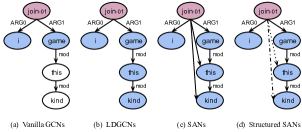
Figure 1: The concept (join-01) in vanilla GCNs is that it only captures information from its immediate neighbors (first-order), while in LDGCNs it can integrate information from neighbors of different order (e.g., second-order and third-order). In SANs, the node collects information from all other nodes, while in structured SANs it is aware of its connected nodes in the original graph.

One type of such GNNs is Graph Convolutional Networks (GCNs; Kipf and Welling 2017). GCNs follow a local information aggregation scheme, iteratively updating the representations of nodes based on their immediate (first-order) neighbors. Intuitively, stacking more convolutional layers in GCNs helps capture more complex interactions (Xu et al., 2018; Guo et al., 2019b). However, prior efforts (Zhu et al., 2019; Cai and Lam, 2020; Wang et al., 2020) have shown that the locality property of existing GCNs precludes efficient non-local information propagation. Abu-El-Haija et al. (2019) further proved that vanilla GCNs are unable to capture feature differences among neighbors from different orders no matter how many layers are stacked. Therefore, Self-Attention Networks (SANs; Vaswani et al. 2017) have been explored as an alternative to capture global dependencies. As shown in Figure 1 (c), SANs associate each node with other nodes such that we model interactions between any two nodes in the graph. Still, this approach ignores the structure of the original graph. Zhu et al. (2019) and Cai and Lam (2020) propose structured SANs that incorporate additional neural components to encode the structural information of the input graph.

Convolutional operations, however, are more computationally efficient than self-attention operations because the computation of attention weights scales quadratically while convolutions scale linearly with respect to the input length (Wu et al., 2019). Therefore, it is worthwhile to explore the possibility of models based on graph convolutions. One potential approach that has been considered is to incorporate information from higher order neighbors, which helps to facilitate non-local information aggregation for node classification (Abu-El-Haija et al., 2018, 2019; Morris et al., 2019). However, simple concatenation of different order representations may not be able to model complex interactions in semantics for text generation (Luan et al., 2019).

We propose to better integrate high-order information, by introducing a novel dynamic fusion mechanism and propose the Lightweight, Dynamic Graph Convolutional Networks (LDGCNs). As shown in Figure 1 (b), nodes in the LDGCN model are able to integrate information from first to third-order neighbors. With the help of the dynamic mechanism, LDGCNs can effectively synthesize information from different orders to model complex interactions in the AMR graph for text generation. Also, LDGCNs require no additional computational overhead, in contrast to vanilla GCN models. We further develop two novel weight sharing strategies based on the group graph convolutions and weight tied convolutions. These strategies allow the LDGCN model to reduce memory usage and model complexity.

Experiments on AMR-to-text generation show that LDGCNs outperform best reported GCNs and SANs trained on LDC2015E86 and LDC2017T10 with significantly fewer parameters. On the large-scale semi-supervised setting, our model is also consistently better than others, showing the effectiveness of the model on a large training set. We release our code and pretrained models at https://github.com/yanzhang92/LDGCNs.

2 Background

Graph Convolutional Networks

Our LDGCN model is closely related to GCNs (Kipf and Welling, 2017) which restrict filters to operate on a first-order neighborhood. Given an AMR graph $\mathcal{G}$ with $n$ concepts (nodes), GCNs associate each concept $v$ with a feature vector $\mathbf{h}_{v}$ $\in$ $\mathbb{R}^{d}$, where $d$ is the feature dimension. $\mathcal{G}$ can be represented by concatenating features of all the concepts, i.e., $\mathbf{H}$=$[\mathbf{h}_{v_{1}},...,\mathbf{h}_{v_{n}}]$. Graph convolutions at $l$-th layer can be defined as:

$$\vspace{-1mm}\mathbf{H}_{l+1}=\phi(\mathbf{A}\mathbf{H}_{l}\mathbf{W}_{l}+\mathbf{b}_{l}),\vspace{-1mm}$$ (1)

where $\mathbf{H}_{l}$ is hidden representations of the $l$-th layer. $\mathbf{W}_{l}$ and $\mathbf{b}_{l}$ are trainable model parameters for the $l$-th layer, $\phi$ is an activation function. $\mathbf{A}$ is the adjacency matrix, $\mathbf{A}_{uv}$=1 if there exists a relation (edge) that goes from concept $u$ to concept $v$.

Self-Attention Networks

Unlike GCNs, SANs (Vaswani et al., 2017) capture global interactions by connecting each concept to all other concepts. Intuitively, the attention matrix can be treated as the adjacency matrix of a fully-connected graph. Formally, SANs take a sequence of representations of $n$ nodes $\mathbf{H}$=$[\mathbf{h}_{v_{1}},...,\mathbf{h}_{v_{n}}]$ as the input. Attention score $\mathbf{A}_{uv}$ between the concept pair ($u$,$v$) is:

$$\vspace{-1mm}\mathbf{A}_{uv} =f(\mathbf{h}_{u},\mathbf{h}_{v})$$ (2)

$$=\mathrm{softmax}(\frac{(\mathbf{h}_{u}\mathbf{W}^{Q})(\mathbf{h}_{v}\textbf{W}^{K})^{T}}{\sqrt{d}})\vspace{-1mm}$$

where $\textbf{W}^{Q}$ and $\textbf{W}^{K}$ are projection parameters. The adjacency matrix $\mathbf{A}$ in GCNs is given by the input AMR graph, while in SANs $\mathbf{A}$ is computed based on $\mathbf{H}$, which neglects the structural information of the input AMR. The number of operations required by graph convolutions scales is found linearly in the input length, whereas they are quadratic for SANs.

Structured SANs

Zhu et al. (2019) and Cai and Lam (2020) extend SAN s by incorporating the relation $\mathbf{r}_{uv}$ between node $u$ and node $v$ in the original graph such that the model is aware of the input structure when computing attention scores:

$$\vspace{-1mm}\mathbf{A}_{uv}=g(\mathbf{h}_{u},\mathbf{h}_{v},\mathbf{r}_{uv})\vspace{-1mm}$$ (3)

where $\mathbf{r}_{uv}$ is obtained based on the shortest relation path between the concept pair $(u,v)$ in the graph. For example, the shortest relation path between (join-01, this) in Figure 1 (d) is [ARG1, mod]. Formally, the path between concept $u$ and $v$ is represented as $s_{uv}$=$[e(u,k_{1}),e(k_{1},k_{2}),...,e(k_{m},v)]$, where $e$ indicates the relation label between two concepts and $k_{1:m}$ are the relay nodes. We have $\mathbf{r}_{uv}=f(s_{uv})$ where $f$ is a sequence encoder, and this can be performed with gated recurrent units (GRUs) or convolutional neural networks (CNNs).

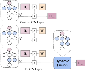
Figure 2: Comparison between vanilla GCNs and LDGCNs. $\mathbf{H}_{l}$ denotes the representation of $l$-th layer. $\mathbf{W}_{l}$ denotes the trainable weights and $\times$ denotes matrix multiplication. Vanilla GCNs take the 1st-order adjacency matrix $\mathbf{A}^{1}$ as the input, which only captures information from one-hop neighbors. LDGCNs take $k$ number of $k$-order adjacency matrix $\mathbf{A}^{k}$ as inputs, $\mathbf{W}_{l}$ is shared for all $\mathbf{A}^{k}$. $k$ is set to 2 here for simplification. A dynamic fusion mechanism is applied to integrate the information from 1- to $k$-hop neighbors.

3 Dynamic Fusion Mechanism

As discussed in Section 2, GCNs are generally more computationally efficient than structured SANs as their computation cost scales linearly and no additional relation encoders are required. However, the locality nature of GCNs precludes efficient non-local information propagation. To address this issue, we propose the dynamic fusion mechanism, which integrates higher order information for better non-local information aggregation. With the help of this mechanism, our model solely based on graph convolutions is able to outperform competitive structured SANs.

Inspired by Gated Linear Units (GLUs; Dauphin et al. 2016), which leverage gating mechanisms (Hochreiter and Schmidhuber, 1997) to dynamically control information flows in the convolutional neural networks, we propose dynamic fusion mechanism (DFM) to integrate information from different orders. DFM allows the model to automatically synthesize information from neighbors at varying degrees of hops away. Similar to GLUs, DFM retains non-linear capabilities of the layer while allowing the gradient to propagate through the linear unit without scaling. Based on this non-linear mixture procedure, DFM is able to control the information flows from a range of orders to specific nodes in the AMR graph. Formally, graph convolutions based on DFM are defined as:

$$\vspace{-1mm}\mathbf{H}_{l+1}= (1-\frac{1}{K-1}\sum\limits_{1<k<K}\mathbf{G}^{(k)}_{l})\odot\phi(\mathbf{A}\mathbf{H}_{l}\mathbf{W}_{l}+\mathbf{b}_{l})$$ (4)

$$+\frac{1}{K-1}\sum\limits_{1<k<K}\mathbf{G}^{(k)}_{l}\odot\phi(\mathbf{A}^{k}\mathbf{H}_{l}\mathbf{W}_{l}+\mathbf{b}_{l}).\vspace{-1mm}$$

where $\mathbf{G}^{(k)}_{l}$ is a gating matrix conditioned on the $k$-th order adjacency matrix $\mathbf{A}^{k}$, namely:

$$\vspace{-1mm}\mathbf{G}^{(k)}_{l}=(1-\lambda^{k})\odot\sigma(\mathbf{A}^{k}\mathbf{H}_{l}\mathbf{W}_{l}+\mathbf{b}_{l}),\vspace{-1mm}$$ (5)

where $\odot$ denotes elementwise product, $\sigma$ denotes the sigmoid function, $\lambda\in(0,1)$ is a scalar, $K\geq 2$ is the highest order used for information aggregation, and $\mathbf{W}_{l}$ denotes trainable weights shared by different $\mathbf{A}^{k}$. Both $\lambda$ and $K$ are hyperparameters.

Computational Overhead

In practice, there is no need to calculate or store $\mathbf{A}^{k}$. $\mathbf{A}^{k}\mathbf{H}_{l}$ is computed with right-to-left multiplication. Specifically, if $k$=3, we calculate $\mathbf{A}^{3}\mathbf{H}_{l}$ as $(\mathbf{A}(\mathbf{A}(\mathbf{A}\mathbf{H}_{l})))$. Since we store $\mathbf{A}$ as a sparse matrix with $m$ non-zero entries as vanilla GCNs, an efficient implementation of our layer takes $O(k_{max}\times m\times d)$ computational time, where $k_{max}$ is the highest order used and $d$ is the feature dimension of $\mathbf{H}_{l}$. Under the realistic assumptions of $k_{max}\ll m$ and $d\ll m$, running an $l$-layer model takes $O(lm)$ computational time. This matches the computational complexity of the vanilla GCNs. On the other hand, DFM does not require additional parameters as the weight matrix is shared over various orders.

Deeper LDGCNs

To further facilitate the non-local information aggregation, we stack several LDGCN layers. In order to stabilize the training, we introduce dense connections (Huang et al., 2017; Guo et al., 2019b) into the LDGCN model. Mathematically, we define the input of the $l$-th layer $\mathbf{\hat{H}}_{l}$ as the concatenation of all node representations produced in layers $1$, $\cdots$, $l-1$:

$$\vspace{-1mm}\mathbf{\hat{H}}_{l}=[\mathbf{H}_{0};\mathbf{H}_{1};...;\mathbf{H}_{l-1}].\vspace{-1mm}$$ (6)

Accordingly, $\mathbf{H}_{l}$ in Eq. 4 is replaced by $\mathbf{\hat{H}}_{l}$.

$$\mathbf{H}_{l+1}= (1-\frac{1}{K-1}\sum\limits_{1<k<K}\mathbf{G}^{(k)}_{l})\odot\phi(\mathbf{A}\mathbf{\hat{H}}_{l}\mathbf{W}_{l}+\mathbf{b}_{l})$$ (7)

$$+\frac{1}{K-1}\sum\limits_{1<k<K}\mathbf{G}^{(k)}_{l}\odot\phi(\mathbf{A}^{k}\mathbf{\hat{H}}_{l}\mathbf{W}_{l}+\mathbf{b}_{l}).$$

where $\textbf{W}_{l}\in\mathbb{R}^{d_{l}\times d}$ and $d_{l}$=$d\times(l-1)$. The model size scales linearly as we increase the depth of the network.

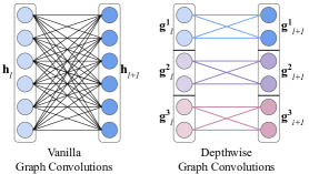
Figure 3: Comparison between vanilla graph convolutions and depthwise graph convolutions. The input and output representation of the $l$-th layer $\mathbf{h}_{l}$ and $\mathbf{h}_{l+1}$ are partitioned into $N$=$3$ disjoint groups.

4 Parameter Saving Strategies

Although we are able to train a very deep LDGCN model, the LDGCN model size increases sharply as we stack more layers, resulting in large model complexity. To maintain a better balance between parameter efficiency and model capacity, we develop two novel parameter saving strategies. We first reduce partial parameters in each layer based on group graph convolutions. Then we further share parameters across all layers based on weight tied convolutions. These strategies allow the LDGCN model to reduce memory usage and model complexity.

4.1 Group Graph Convolutions

Group convolutions have been used to build efficient networks for various computer vision tasks as they can better integrate feature maps (Xie et al., 2017; Li et al., 2019b) and have lower computational costs (Howard et al., 2017; Zhang et al., 2017) compared to vanilla convolutions. In order to reduce the model complexity in the deep LDGCN model, we extend group convolutions to GCNs by introducing group convolutions along two directions: depthwise and layerwise.

Depthwise Graph Convolutions:

As discussed in Section 2, graph convolutions operate on the features of $n$ nodes $\mathbf{H}\in\mathbb{R}^{n\times d}$. For simplicity, we assume $n$=1, the input and output representation of the $l$-th layer are $\mathbf{h}_{l}\in\mathbb{R}^{d_{l}}$ and $\mathbf{h}_{l+1}\in\mathbb{R}^{d_{l+1}}$, respectively. As shown in Figure 3, the size of the weight matrix $\mathbf{W}_{l}$ in a vanilla graph convolutions is $d_{l}\times d_{l+1}$. In depthwise graph convolutions, $\mathbf{h}_{l}$ is partitioned into $N$ mutually exclusive groups $\{\mathbf{g}^{1}_{l}$,…,$\mathbf{g}^{N}_{l}\}$. The weight $\mathbf{W}_{l}$ of each layer is also partitioned into $N$ mutually exclusive groups $\mathbf{W}^{1}_{l}$,…,$\mathbf{W}^{N}_{l}$. The dimension of each weight is $\frac{d_{l}}{N}\times\frac{d_{l+1}}{N}$. Finally, we obtain the output representation $\mathbf{h}_{l+1}$ by concatenating $N$ groups of outputs [$\mathbf{g}^{1}_{l+1}$;…;$\mathbf{g}^{N}_{l+1}$]. Now the parameters of each layer can be reduced by a factor of $N$, to $\frac{d_{l}\times d_{l+1}}{N}$.

Layerwise Graph Convolutions:

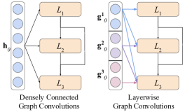
Figure 4: Comparison between vanilla graph convolutions and layerwise graph convolutions. The input representation $\mathbf{h}_{0}$ is partitioned into $M$=$3$ disjoint groups.

These group convolutions are built based on densely connected graph convolutions (Guo et al., 2019b). As shown in Figure 4, each layer takes the concatenation of outputs from all preceding layers as its input. For example, layer $L_{2}$ takes the concatenation of [$\mathbf{h}_{0};\mathbf{h}_{1}$] as its input. Guo et al. (2019b) further adopt a dimension shrinkage strategy. Assume $\mathbf{h}_{0}\in\mathbb{R}^{d}$ and that the network has $L$ layers. The dimension of output for each layer is set to $\frac{d}{L}$. Finally, we concatenate the output of $L$ layers [$\mathbf{h}_{1};...;\mathbf{h}_{L}$] to form the final representation $h_{final}\in\mathbb{R}^{d}$. Therefore, the size of weight matrix for $l$-th layer is $(d+\frac{d\times(l-1)}{L})\times\frac{d}{L}$.

Notice that main computation cost originates in the computation of $\mathbf{h}_{0}$ as it has a large dimension and it is concatenated to the input of each layer. In layerwise graph convolutions however, we improve the parameter efficiency by dividing the input representation $\mathbf{h}_{0}$ into $M$ groups $\{\mathbf{g}^{1}_{0}$,…$\mathbf{g}^{M}_{0}\}$, where $M$ equals the total number of layers $L$. The first group $\mathbf{g}^{1}_{0}$ is fed to all $L$ layers, and the second group $\mathbf{g}^{2}_{0}$ is fed to ($L$-1) layers, so on and so forth. Accordingly, the size of weight matrix for the $l$-th layer is $(\frac{d\times(2l-1)}{L})\times\frac{d}{L}$.

Formally, we partition the input representations of $n$ concept $\mathbf{H}_{0}\in\mathbb{R}^{n\times d}$ to the first layer into $M$ groups $\{\mathbf{G}^{1}_{0},...,\mathbf{G}^{M}_{0}\}$, where the size of each group is $n\times\frac{d}{M}$. Accordingly, we modify the input of the $l$-th layer $\mathbf{\hat{H}}_{l}$ in Eq. 6 as:

$$\mathbf{\hat{H}}_{l}=[\mathbf{G}^{1}_{0};...;\mathbf{G}^{M}_{0};\mathbf{H}_{1};...;\mathbf{H}_{l-1}]$$ (8)

In practice, we combine these two convolutions together to further reduce the model size. For example, assume the size of the input is $d$=360 and the number of layers is $L$=6. The size of the weight matrix for the first layer ($l$=1) is $(d+\frac{d\times(l-1)}{L})\times\frac{d}{L}$=$360\times 60$. Assume we set $N$=3 for depthwise graph convolutions and $M$=6 for layerwise graph convolutions. We first use layerwise graph convolutions by dividing the input into 6 groups, where each one has the size $\frac{d}{M}$=60. Then we feed the first group to the first layer. Next we use depthwise graph convolutions to further split the input into 3 groups. We now have 3 weight matrices for the first layer, each one with the size $\frac{d\times(2l-1)}{M}\times\frac{d}{M\times N}$= $20\times 20$. With the increase of the feature dimension $d$ and the number of layer $L$, more prominent parameter efficiency can be observed.

4.2 Weight Tied Convolutions

We further adopt a more aggressive strategy where parameters are shared across all layers. This further significantly reduces the size of the model. Theoretically, weight tied networks can be unrolled to any depth, typically with improved feature abstractions as depth increases (Bai et al., 2019a). Recently, weight tied SANs were explored to regularize the training and help with generalization (Dehghani et al., 2019; Lan et al., 2020). Mathematically, Eq. 1 can be rewritten as:

$$\vspace{-1mm}\mathbf{H}_{l+1}=\phi(\mathbf{A}\mathbf{\hat{H}}_{l}\mathbf{W}+\mathbf{b}),\vspace{-1mm}$$ (9)

where $\mathbf{W}$ and $\mathbf{b}$ are shared parameters for all convolutional layers. To stabilize training, a gating mechanism was introduced to graph neural networks in order to build graph recurrent networks (Li et al., 2016; Song et al., 2018), where parameters are shared across states (time steps). However, the graph convolutional structure is very deep (e.g., 36 layers). Instead, we adopt a jumping connection (Xu et al., 2018), which forms the final representation $\mathbf{H}_{final}$ based on the output of all layers. This connection mechanism can be considered deep supervision (Lee et al., 2015; Bai et al., 2019b) for training deep convolutional neural networks. Formally, the $\mathbf{H}_{final}$ of LDGCNs which have $L$ layer is obtained by: $\mathbf{H}_{final}=\mathcal{F}(\mathbf{\hat{H}}_{L},...,\mathbf{\hat{H}}_{1})$, where $\mathcal{F}$ is a linear transformation.

5 Experiments

5.1 Setup

We evaluate our model on the LDC2015E86 (AMR1.0), LDC2017T10 (AMR2.0) and LDC2020T02 (AMR3.0) datasets, which have 16,833, 36,521 and 55,635 instances for training, respectively. Both AMR1.0 and AMR2.0 have 1,368 instances for development, and 1,371 instances for testing. AMR3.0 has 1,722 instances for development and 1,898 instances for testing. Following Zhu et al. (2019), we use byte pair encodings Sennrich et al. (2016) to deal with rare words.

Following Guo et al. (2019b), we stack 4 LDGCN blocks as the encoder of our model. Each block consists of two sub-blocks where the bottom one contains 6 layers and the top one contains 3 layers. The hidden dimension of LDGCN model is 480. Other model hyperparameters are set as $\lambda$=0.7, $K$=2 for dynamic fusion mechanism, $N$=2 for depthwise graph convolutions and $M$=6 and 3 for layerwise graph convolutions for the bottom and top sub-blocks, respectively. For the decoder, we employ the same attention-based LSTM as in previous work (Beck et al., 2018; Guo et al., 2019b; Damonte and Cohen, 2019). Following Wang et al. (2020), we use a transformer as the decoder for large-scale evaluation. For fair comparisons, we use the same optimization and regularization strategies as in Guo et al. (2019b). All hyperparameters are tuned on the development set.

Model	Type	AMR2015				AMR2017
		B	C	M	#P	B	C	M	#P
Seq2Seq Cao and Clark (2019)	Single	23.5	-	-	-	26.8	-	-	-
GraphLSTM Song et al. (2018)	Single	23.3	-	-	-	24.9	-	-	-
GGNNs Beck et al. (2018)	Single	-	-	-	-	23.3	50.4	-	28.3M
GCNLSTM Damonte and Cohen (2019)	Single	24.4	-	23.6	-	24.5	-	24.1	030.8M‡
DCGCN Guo et al. (2019b)	Single	25.7	0 54.5‡	031.5‡	018.6M‡	27.6	57.3	34.0	19.1M
DualGraph Ribeiro et al. (2019)	Single	24.3	053.8‡	30.5	060.3M‡	27.9	058.0‡	33.2	061.7M‡
Seq2Seq Konstas et al. (2017)	Ensemble	-	-	-	-	26.6	52.5	-	142M
GGNNs Beck et al. (2018)	Ensemble	-	-	-	-	27.5	53.5	-	141M
DCGCN Guo et al. (2019b)	Ensemble	-	-	-	-	30.4	59.6	-	92.5M
Transformer Zhu et al. (2019)	Single	25.5	59.9	33.1	49.1M	27.4	61.9	34.6	-
GT_Dual Wang et al. (2020)	Single	25.9	-	-	19.9M	29.3	59.0	-	19.9M
GT_GRU Cai and Lam (2020)	Single	27.4	56.4	32.9	30.8M	29.8	59.4	35.1	32.2M
GT_SAN Zhu et al. (2019)	Single	29.7	060.7‡	35.5	49.3M	31.8	061.8‡	36.4	054.0M‡
LDGCN_WT	Single	28.6	58.5	33.1	10.6M	31.9	61.2	36.3	11.8M
LDGCN_GC	Single	30.8	61.8	36.4	12.9M	33.6	63.2	37.5	13.6M

Table 1: Main results on AMR-to-text generation. B, C, M and #P denote BLEU, CHRF++, METEOR and the model size in terms of parameters, respectively. Results with $\ddagger$ are obtained from the authors. We also conduct the statistical significance tests by following (Zhu et al., 2019). All our proposed systems are significant over the baseline at $p<0.01$, tested by bootstrap resampling (Koehn, 2004).

Model	#P	External	B
Seq2Seq (Konstas et al., 2017)	-	2M	32.3
Seq2Seq (Konstas et al., 2017)	-	20M	33.8
GraphLSTM (Song et al., 2018)	-	2M	33.6
Transformer Wang et al. (2020)	-	2M	35.1
GT_Dual Wang et al. (2020)	78.4M	2M	36.4
LDGCN_GC	23.2M	0.5M	36.0
LDGCN_WT	20.8M	0.5M	36.8

Table 2: Results on AMR1.0 with external training data. ^‡ denotes the ensemble model.

For evaluation, we report BLEU scores Papineni et al. (2002), CHRF++ Popovic (2017) scores and METEOR scores Denkowski and Lavie (2014) with additional human evaluation results.

5.2 Main Results

We consider two kinds of baseline models: 1) models based on Recurrent Neural Networks  Konstas et al. (2017); Cao and Clark (2019) and Graph Neural Networks (GNNs) Song et al. (2018); Beck et al. (2018); Damonte and Cohen (2019); Guo et al. (2019b); Ribeiro et al. (2019). These models use an attention-based LSTM decoder. 2) models based on SANs Zhu et al. (2019) and structured SANs Cai and Lam (2020); Zhu et al. (2019); Wang et al. (2020). Specifically, Zhu et al. (2019) leverage additional SANs to incorporate the relational encoding whereas Cai and Lam (2020) use GRUs. Additional results of ensemble models are also included. The results are reported in Table 1. Our model has two variants based on different parameter saving strategies, including LDGCN_WT (weight tied) and LDGCN_GC (group convolutions), and both of them use the dynamic fusion mechanism (DFM).

LDGCN v.s. Structured SANs.

Compared to state-of-the-art structured SANs (GT_SAN), the performance of LDGCN_GC is 1.1 and 1.8 BLEU points higher on AMR1.0 and AMR2.0, respectively. Moreover, LDGCN_GC requires only about a quarter of the number of parameters (12.9M vs 49.0M, and 13.6M vs 54.0M). Our more lightweight variant LDGCN_WT achieves better BLEU scores than GT_SAN on AMR2.0 while using only 1/5 of their model parameters. However, LDGCN_WT obtains lower scores on AMR1.0 than GT_SAN. We hypothesize that weight tied convolutions require more data to train as we observe severe oscillations when training the model on the small AMR1.0 dataset. The oscillation is reduced when we train it on the larger AMR2.0 dataset and the semi-supervised dataset.

Model	B	C	M	#P
GGNNs (Beck et al., 2018)	26.7†	57.2†	33.1†	30.9M†
DCGCN (Guo et al., 2019b)	29.8‡	59.9‡	35.6‡	22.2M‡
LDGCN_WT	33.0	62.6	36.5	11.5M
LDGCN_GC	34.3	63.7	38.2	14.3M

Table 3: Results on the AMR3.0. B, C, M and #P denote BLEU, CHRF++, METEOR and the model size in terms of parameters, respectively. The results with $\dagger$ are based on open implementations, while the results with $\ddagger$ are obtained from the authors.

LDGCN v.s. Other GNNs.

Both LDGCN models significantly outperform GNN-based models. For example, LDGCN_GC surpasses DCGCN by 5.1 points on AMR1.0 and surpasses DualGraph by 5.7 points on AMR2.0. Moreover, the single LDGCN model achieves consistently better results than previous ensemble GNN-based models in BLEU, CHRF++ and METEOR scores. In particular, on AMR2.0, LDGCN_WT obtains 1.5 BLEU points higher than the DCGCN ensemble model, while requiring only about 1/8 of the number of parameters. We also evaluate our model on the latest AMR3.0 dataset. Results are shown in Table 3. LDGCN_WT and LDGCN_GC consistently outperform GNN-based models including DCGCN and GGNNs on this larger dataset. These results suggest that LDGCN can learn better representation more efficiently.

Large-scale Evaluation.

We further evaluate LDGCNs on a large-scale dataset. Following Wang et al. (2020), we first use the additional data to pretrain the model, then finetune it on the gold data. Evaluation results are reported in Table.2. Using 0.5M data, LDGCN_WT outperforms all models including structured SANs with 2M additional data. These results show that our model is more effective in terms of using a larger dataset. Interestingly, LDGCN_WT consistently outperforms LDGCN_GC under this setting. Unlike training the model on AMR1.0, training LDGCN_WT on the large-scale dataset has fewer oscillations, which confirms our hypothesis that sufficient data acts as a regularizer to stabilize the training process of weight tied models.

5.3 Development Experiments

We conduct an ablation study to demonstrate how dynamic fusion mechanism and parameter saving strategies are beneficial to the lightweight model with better performance based on development of experimental results on AMR1.0. Results are shown in Table 4. DeepGCN is the model with dense connections (Huang et al., 2017; Guo et al., 2019b). DeepGCN+GC+DF and DeepGCN+WT+DF are essentially LDGCN_GC and LDGCN_WT models in Section 5.2, respectively.

Model	#Parameters	BLEU
DeepGCN	19.9M	29.3
DeepGCN+DF	19.9M	30.4
DeepGCN+GC	12.9M	29.0
DeepGCN+GC+DF (LDGCN_GC)	12.9M	30.3
DeepGCN+WT	10.6M	27.4
DeepGCN+WT+DF (LDGCN_WT)	10.6M	28.3

Table 4: Comparisons between baselines. +DF denotes dynamic fusion mechanism. +WT and +GC refer to weight tied and group convolutions, respectively.

Model	Inference Speed
Transformer	1.00x
DeepGCN	1.21x
LDGCN_WT	1.22x
LDGCN_GC	1.17x

Table 5: Speed comparisons between baselines. For inference speed, the higher the better. Implementations are based on MXNet (Chen et al., 2015) and the Sockeye neural machine translation toolkit (Felix et al., 2017). Results on speed are based on beam size 10, batch size 30 on an NVIDIA RTX 1080 GPU.

Dynamic Fusion Mechanism.

The performance of DeepGCN+DF is 1.1 BLEU points higher than DeepGCN, which demonstrates that our dynamic fusion mechanism is beneficial for graph encoding when applied alone. Adding the group graph convolutions strategies gives a BLEU score of 30.3, which is only 0.1 points lower than DeepGCN+DF. This result shows that the representation learning ability of the dynamic fusion mechanism is robust against parameter sharing and reduction. We also observe that the mechanism helps to alleviate oscillation when training the weight tied model. DeepGCN+WT+DF achieves better results than DeepGCN+WT, which is hard to converge when training it on the small AMR1.0 dataset.

Parameter Saving Strategy.

Table 4 demonstrates that although the performance of DeepGCN+GC is only 0.3 BLEU points lower than that of DeepGCN, DeepGCN+GC only requires $65\%$ of the number of parameters of DeepGCN. Furthermore, by introducing the dynamic fusion mechanism, the performance of DeepGCN+GC is improved greatly and is in fact on par with DeepGCN. Also, DeepGCN+GC+DF does not rely on any kind of self-attention layers, hence, its number of parameters is much smaller than that of graph transformers, i.e., DeepGCN+GC+DF only needs $1/4$ to $1/3$ the number of parameters of graph transformers, as shown in Table 1. On the other hand, DeepGCN+WT is more efficient than DeepGCN+GC. As shown in Table 2, with an increase in training data, more prominent parameter efficiency can be observed.

Time Cost Analysis.

As shown in the Table 5, all three GCN-based models outperform the SAN-based model in terms of speed because the computation of attention weights scales quadratically while convolutions scale linearly with respect to the input graph size. LDGCN_GC is slightly slower than the other two models, since it requires additional tensor split operations. We believe that state-of-the-art structured SANs are also strictly slower than vanilla SANs, as they require additional neural components, such as GRUs, to encode structural information in the AMR graph. In summary, our model not only has better parameter efficiency, but also lower time costs.

5.4 Human Evaluation

We further assess the quality of the generated sentences with human evaluation. Following Ribeiro et al. (2019), two evaluation criteria are used: (i) meaning similarity: how close in meaning the generated text is to the gold sentence; (ii) readability: how well the generated sentence reads. We randomly select 100 sentences generated by 4 models. 30 human subjects rate the sentences on a 0-100 rating scale. The evaluation is conducted separately and subjects were first given brief instructions explaining the criteria of assessment. For each sentence, we collect scores from 5 subjects and average them. Models are ranked according to the mean of sentence-level scores. Also, we apply a quality control step filtering subjects who do not score some faked and known sentences properly.

As shown in Table 6, LDGCN_GC has better human rankings in terms of both meaning similarity and readability than the state-of-the art GNN-based (DualGraph) and SAN-based model (GT_SAN). DeepGCN without dynamic fusion mechanism obtains lower scores than GT_SAN, which further confirms that synthesizing higher order information helps in learning better graph representations.

Model	Similarity	Readability
DualGraph (Ribeiro et al., 2019)	65.07	68.78
GT_SAN (Zhu et al., 2019)	69.63	72.23
DeepGCN	68.91	71.45
LDGCN_GC	71.92	74.16

Table 6: Human evaluation. We also perform significance tests by following (Ribeiro et al., 2019). Results are statistically significant with $p<0.05$.

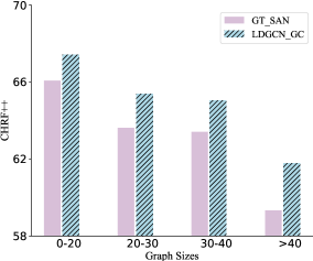
Figure 5: Performance against graph sizes.

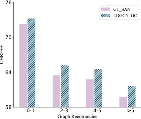
Figure 6: Performance against graph re-entrancies.

5.5 Additional Analysis

To further reveal the source of performance gains, we perform additional analysis based on the characteristics of AMR graphs, i.e., graph size and graph reentrancy  Damonte and Cohen (2019); Damonte et al. (2020). All experiments are conducted on the AMR2.0 test set and CHRF++ scores are reported.

Graph Size.

As shown in Figure 5, the size of AMR graphs is partitioned into four categories (($0$, $20$], ($20$, $30$], ($30$, $40$], $>40$), Overall, LDGCN_GC outperforms the best-reported GT_SAN model across all graph sizes, and the performance gap becomes more profound with the increase of graph sizes. Although both models have sharp performance degradation for extremely large graphs ($>40$), the performance of LDGCN_GC is more stable. Such a result suggests that our model can better deal with large graphs with more complicated structures.

Graph re-entrancies.

Reentrancies describe the co-references and control structures in AMR graphs. A graph is considered more complex if it contains more re-entrancies. In Figure 6, we show how the LDGCN_GC and GT_SAN generalize to different scales of reentrancies. Again, LDGCN_GC consistently outperforms GT_SAN and the performance gap becomes noticeably wider when the number of re-entrancies increases. These results suggest that our model can better model the complex dependencies in AMR graphs.

(m / multi-sentence

000 :snt1 (t / trust-01

000000 :ARG2 (i / i))

000 :snt2 (g / good-02

000000 :ARG1 (g2 / get-01

000000000 :ARG1 (t2 / thing

000000000000 :mod (t3 / this))

000000000 :time e.10,12 (e / early

000000000000 :degree (m2 / most)

0000000 00000:compared-to (p / possible-01

000000000000000 :ARG1 g2))

000000000 :ARG1-of (i2 / instead-of-91

000000000000 :ARG2 (l / let-01

000000000000000 :ARG1 (w / worsen-01

000000000000000000 :ARG1 t2

000000000000000000 :mod (e2 / even)))))

0000000 :degree e.5 (m3 / more)))

Reference: trust me , it ’s better to get these things as early

as possible rather than let them get even worse .

DualGraph: so to me , this is the best thing to get these

things as they can , instead of letting it even worse .

DeepGCN: i trust me , it ’s better that these things get

in the early than letting them even get worse .

GT_SAN: trust me , this is better to get these

things , rather than let it even get worse .

LDGCN_GC: trust me . better to get these things as early

as possible , rather than letting them even make worse .

Table 7: An example of AMR graph and generated sentences by different models.

Case Study.

Table 7 shows the generated sentence of an AMR graph from four models together with the gold reference. The phrase “trust me” is the beginning of the sentence. DualGraph fails to decode it. On the other hand, GT_SAN successfully generates the second half of the sentence, i.e., “rather than let them get even worse”, but it fails to capture the meaning of word “early” in its output, which is a critical part. DeepGCN parses both “early” and “get even worse” in the results. However, the readability of the generated sentence is not satisfactory. Compared to baselines, LDGCN is able to produce the best result, which has a correct starting phrase and captures the semantic meaning of critical words such as “early” and “get even worse” while also attaining good readability.

6 Related Work

Graph convolutional networks (Kipf and Welling, 2017) have been widely used as the structural encoder in various NLP applications including question answering (De Cao et al., 2019; Lin et al., 2019), semantic parsing (Bogin et al., 2019a, b) and relation extraction (Guo et al., 2019a, 2020).

Early efforts for AMR-to-text generation mainly include grammar-based models (Flanigan et al., 2016; Song et al., 2017) and sequence-based models (Pourdamghani et al., 2016; Konstas et al., 2017; Cao and Clark, 2019), discarding crucial structural information when linearising the input AMR graph. To solve that, various GNNs including graph recurrent networks (Song et al., 2018; Ribeiro et al., 2019) and graph convolutional networks (Damonte and Cohen, 2019; Guo et al., 2019b) have been used to encode the AMR structure. Though GNNs are able to operate directly on graphs, the locality nature of them precludes efficient information propagation (Abu-El-Haija et al., 2018, 2019; Luan et al., 2019). Larger and deeper models are required to model the complex non-local interactions (Xu et al., 2018; Li et al., 2019a). More recently, SAN-based models (Zhu et al., 2019; Cai and Lam, 2020; Wang et al., 2020) outperform GNN-based models as they are able to capture global dependencies. Unlike previous models, our local, yet efficient model, based solely on graph convolutions, outperforms competitive structured SANs while using a significantly smaller model.

7 Conclusion

In this paper, we propose LDGCNs for AMR-to-text generation. Compared with existing GCNs and SANs, LDGCNs maintain a better balance between parameter efficiency and model capacity. LDGCNs outperform state-of-the-art models on AMR-to-text generation. In future work, we would like to investigate methods to stabilize the training of weight tied models and apply our model on other tasks in Natural Language Generation.

References

- Abu-El-Haija et al. (2018) Sami Abu-El-Haija, Amol Kapoor, Bryan Perozzi, and Joonseok Lee. 2018. N-gcn: Multi-scale graph convolution for semi-supervised node classification. In Proc. of UAI.
- Abu-El-Haija et al. (2019) Sami Abu-El-Haija, Bryan Perozzi, Amol Kapoor, Hrayr Harutyunyan, Nazanin Alipourfard, Kristina Lerman, Greg Ver Steeg, and Aram Galstyan. 2019. Mixhop: Higher-order graph convolutional architectures via sparsified neighborhood mixing. In Proc. of ICML.
- Bai et al. (2019a) Shaojie Bai, J. Zico Kolter, and Vladlen Koltun. 2019a. Deep equilibrium models. In Proc. of NeurIPS.
- Bai et al. (2019b) Shaojie Bai, J. Zico Kolter, and Vladlen Koltun. 2019b. Trellis networks for sequence modeling. In Proc. of ICLR.
- Banarescu et al. (2013) Laura Banarescu, Claire Bonial, Shu Cai, Madalina Georgescu, Kira Griffitt, Ulf Hermjakob, Kevin Knight, Philipp Koehn, Martha Palmer, and Nathan Schneider. 2013. Abstract meaning representation for sembanking. In Proc. of LAW@ACL.
- Beck et al. (2018) Daniel Beck, Gholamreza Haffari, and Trevor Cohn. 2018. Graph-to-sequence learning using gated graph neural networks. In Proc. of ACL.
- Bogin et al. (2019a) Ben Bogin, Matt Gardner, and Jonathan Berant. 2019a. Global reasoning over database structures for text-to-sql parsing. In Proc. of EMNLP.
- Bogin et al. (2019b) Ben Bogin, Matt Gardner, and Jonathan Berant. 2019b. Representing schema structure with graph neural networks for text-to-sql parsing. In Proc. of ACL.
- Cai and Lam (2020) Deng Cai and Wai Lam. 2020. Graph transformer for graph-to-sequence learning. In Proc. of AAAI.
- Cao and Clark (2019) Kris Cao and Stephen Clark. 2019. Factorising AMR generation through syntax. In Proc. of NAACL-HLT.
- Chen et al. (2015) Tianqi Chen, Mu Li, Yutian Li, Min Lin, Naiyan Wang, Minjie Wang, Tianjun Xiao, Bing Xu, Chiyuan Zhang, and Zheng Zhang. 2015. Mxnet: A flexible and efficient machine learning library for heterogeneous distributed systems. arXiv preprint.
- Damonte and Cohen (2019) Marco Damonte and Shay B. Cohen. 2019. Structural neural encoders for AMR-to-text generation. In Proc. of NAACL-HLT.
- Damonte et al. (2020) Marco Damonte, Ida Szubert, Shay B. Cohen, and Mark Steedman. 2020. The role of reentrancies in abstract meaning representation parsing. In Findings of EMNLP.
- Dauphin et al. (2016) Yann Dauphin, Angela Fan, Michael Auli, and David Grangier. 2016. Language modeling with gated convolutional networks. In Proc. of ICML.
- De Cao et al. (2019) Nicola De Cao, Wilker Aziz, and Ivan Titov. 2019. Question answering by reasoning across documents with graph convolutional networks. In Proc. of NAACL-HLT.
- Dehghani et al. (2019) Mostafa Dehghani, Stephan Gouws, Oriol Vinyals, Jakob Uszkoreit, and Lukasz Kaiser. 2019. Universal transformers. In Proc. of ICLR.
- Denkowski and Lavie (2014) Michael J. Denkowski and Alon Lavie. 2014. Meteor universal: Language specific translation evaluation for any target language. In Proc. of WMT@ACL.
- Felix et al. (2017) Hieber Felix, Domhan Tobias, Denkowski Michael, Vilar David, Sokolov Artem, Clifton Ann, and Post Matt. 2017. Sockeye: A toolkit for neural machine translation. arXiv preprint.
- Flanigan et al. (2016) Jeffrey Flanigan, Chris Dyer, Noah A. Smith, and Jaime G. Carbonell. 2016. Generation from abstract meaning representation using tree transducers. In Proc. of NAACL-HLT.
- Guo et al. (2020) Zhijiang Guo, Guoshun Nan, Wei Lu, and Shay B. Cohen. 2020. Learning latent forests for medical relation extraction. In Proc. of IJCAI.
- Guo et al. (2019a) Zhijiang Guo, Yan Zhang, and Wei Lu. 2019a. Attention guided graph convolutional networks for relation extraction. In Proc. of ACL.
- Guo et al. (2019b) Zhijiang Guo, Yan Zhang, Zhiyang Teng, and Wei Lu. 2019b. Densely connected graph convolutional networks for graph-to-sequence learning. Transactions of the Association for Computational Linguistics, 7:297–312.
- Hochreiter and Schmidhuber (1997) Sepp Hochreiter and Jürgen Schmidhuber. 1997. Long short-term memory. Neural computation, 9(8):1735–1780.
- Howard et al. (2017) Andrew G. Howard, Menglong Zhu, Bo Chen, Dmitry Kalenichenko, Weijun Wang, Tobias Weyand, Marco Andreetto, and Hartwig Adam. 2017. Mobilenets: Efficient convolutional neural networks for mobile vision applications. ArXiv, abs/1704.04861.
- Huang et al. (2017) Gao Huang, Zhuang Liu, Laurens van der Maaten, and Kilian Q. Weinberger. 2017. Densely connected convolutional networks. In Proc. of CVPR.
- Kipf and Welling (2017) Thomas N. Kipf and Max Welling. 2017. Semi-supervised classification with graph convolutional networks. In Proc. of ICLR.
- Koehn (2004) Philipp Koehn. 2004. Statistical significance tests for machine translation evaluation. In Proc. of EMNLP.
- Konstas et al. (2017) Ioannis Konstas, Srinivasan Iyer, Mark Yatskar, Yejin Choi, and Luke S. Zettlemoyer. 2017. Neural AMR: Sequence-to-sequence models for parsing and generation. In Proc. of ACL.
- Lan et al. (2020) Zhen-Zhong Lan, Mingda Chen, Sebastian Goodman, Kevin Gimpel, Piyush Sharma, and Radu Soricut. 2020. Albert: A lite bert for self-supervised learning of language representations. In Proc. of ICLR.
- Lee et al. (2015) Chen-Yu Lee, Saining Xie, Patrick W. Gallagher, Zhengyou Zhang, and Zhuowen Tu. 2015. Deeply-supervised nets. In Proc. of AISTATS.
- Li et al. (2019a) Guohao Li, Matthias Müller, Ali Thabet, and Bernard Ghanem. 2019a. Can gcns go as deep as cnns? In Proc. of ICCV.
- Li et al. (2019b) Xiang Li, Wenhai Wang, Xiaolin Hu, and Jian Yang. 2019b. Selective kernel networks. In Proc. of CVPR.
- Li et al. (2016) Yujia Li, Daniel Tarlow, Marc Brockschmidt, and Richard S. Zemel. 2016. Gated graph sequence neural networks. In Proc. of ICLR.
- Lin et al. (2019) Bill Yuchen Lin, Xinyue Chen, Jamin Chen, and Xiang Ren. 2019. Kagnet: Knowledge-aware graph networks for commonsense reasoning. In Proc. of EMNLP.
- Luan et al. (2019) Sitao Luan, Mingde Zhao, Xiao-Wen Chang, and Doina Precup. 2019. Break the ceiling: Stronger multi-scale deep graph convolutional networks. In Proc. of NeurIPS.
- Morris et al. (2019) Christopher Morris, Martin Ritzert, Matthias Fey, William L. Hamilton, Jan Eric Lenssen, Gaurav Rattan, and Martin Grohe. 2019. Weisfeiler and leman go neural: Higher-order graph neural networks. In Proc. of AAAI.
- Papineni et al. (2002) Kishore Papineni, Salim Roukos, Todd Ward, and Wei-Jing Zhu. 2002. Bleu: a method for automatic evaluation of machine translation. In Proc. of ACL.
- Popovic (2017) Maja Popovic. 2017. chrf++: words helping character n-grams. In Proc. of WMT@ACL.
- Pourdamghani et al. (2016) Nima Pourdamghani, Kevin Knight, and Ulf Hermjakob. 2016. Generating english from abstract meaning representations. In Proc. of INLG.
- Ribeiro et al. (2019) Leonardo Filipe Rodrigues Ribeiro, Claire Gardent, and Iryna Gurevych. 2019. Enhancing AMR-to-text generation with dual graph representations. In Proc. of EMNLP.
- Sennrich et al. (2016) Rico Sennrich, Barry Haddow, and Alexandra Birch. 2016. Neural machine translation of rare words with subword units. In Proc. of ACL.
- Song et al. (2017) Linfeng Song, Xiaochang Peng, Yue Zhang, Zhiguo Wang, and Daniel Gildea. 2017. AMR-to-text generation with synchronous node replacement grammar. In Proc. of ACL.
- Song et al. (2018) Linfeng Song, Yue Zhang, Zhiguo Wang, and Daniel Gildea. 2018. A graph-to-sequence model for AMR-to-text generation. In Proc. of ACL.
- Vaswani et al. (2017) Ashish Vaswani, Noam Shazeer, Niki Parmar, Jakob Uszkoreit, Llion Jones, Aidan N. Gomez, Lukasz Kaiser, and Illia Polosukhin. 2017. Attention is all you need. In Proc. of NeurIPS.
- Wang et al. (2020) Tianming Wang, Xiaojun Wan, and Hanqi Jin. 2020. AMR-to-text generation with graph transformer. Transactions of the Association for Computational Linguistics, 8:19–33.
- Wu et al. (2019) Felix Wu, Angela Fan, Alexei Baevski, Yann N Dauphin, and Michael Auli. 2019. Pay less attention with lightweight and dynamic convolutions. In Proc. of ICLR.
- Xie et al. (2017) Saining Xie, Ross B. Girshick, Piotr Dollár, Zhuowen Tu, and Kaiming He. 2017. Aggregated residual transformations for deep neural networks. In Proc. of CVPR.
- Xu et al. (2018) Keyulu Xu, Chengtao Li, Yonglong Tian, Tomohiro Sonobe, Ken ichi Kawarabayashi, and Stefanie Jegelka. 2018. Representation learning on graphs with jumping knowledge networks. In Proc. of ICML.
- Zhang et al. (2017) Xiangyu Zhang, Xinyu Zhou, Mengxiao Lin, and Jian Sun. 2017. Shufflenet: An extremely efficient convolutional neural network for mobile devices. In Proc. of CVPR.
- Zhu et al. (2019) Jie Zhu, Junhui Li, Muhua Zhu, Longhua Qian, Min Zhang, and Guodong Zhou. 2019. Modeling graph structure in transformer for better AMR-to-text generation. In Proc. of EMNLP.