Pragmatically Informative Color Generation
by Grounding Contextual Modifiers

Abstract

Grounding language in contextual information is crucial for fine-grained natural language understanding. One important task that involves grounding contextual modifiers is color generation. Given a reference color “green”, and a modifier “bluey”, how does one generate a color that could represent “bluey green”? We propose a computational pragmatics model that formulates this color generation task as a recursive game between speakers and listeners. In our model, a pragmatic speaker reasons about the inferences that a listener would make, and thus generates a modified color that is maximally informative to help the listener recover the original referents. In this paper, we show that incorporating pragmatic information provides significant improvements in performance compared with other state-of-the-art deep learning models where pragmatic inference and flexibility in representing colors from a large continuous space are lacking. Our model has an absolute 98% increase in performance for the test cases where the reference colors are unseen during training, and an absolute 40% increase in performance for the test cases where both the reference colors and the modifiers are unseen during training.

1 Introduction

When describing colors, people rely on comparative adjectives such as “pale”, or “bright” Lassiter and Goodman (2017). Understanding how these comparative words modify the referent color, it requires extensive language grounding, in this case in color space Monroe et al. (2017). For instance, understanding (i.e., correctly generating) a color that corresponds to “pale yellow” requires some knowledge about the meaning of “yellow” and “pale” in color space, and how the latter modifier modifies the former referent color. This is a difficult and underspecified task, because modifiers like “pale” are vague, and the strength and effect of a modifier may also depend on the color it is modifying. Understanding such modifiers and how they are grounded in image space is imperative for fine-grained attribute learning in many computer vision tasks Farhadi et al. (2009); Russakovsky and Fei-Fei (2010); Vedaldi et al. (2014).

Figure 1: Examples of the color modification task, shown in RGB space. Given the reference color (Ref. Color), the modifier changes the color towards a target color. We represent this modification by going from left to right of the colored bar; the target color is shown at the right-end of the bar. The reference color for the top row is green, and purple for the middle and bottom rows.

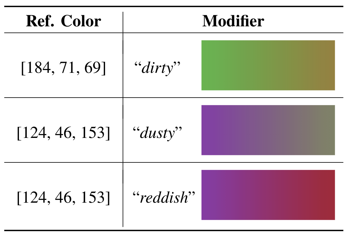
Color provides a simple and tractable space in which to study natural language grounding. Monroe et al. (2017) found that when asked to describe a reference color presented with similar distractors, speakers often rely on comparative adjectives to describe it, rather than relying on context-independent descriptions. Others have also studied contextual dependence and vagueness in human-generated color descriptions Egré et al. (2013); McMahan and Stone (2015). In contrast to these papers, Winn and Muresan (2018) proposed a new paradigm focusing on using machine learning to produce grounded comparative adjectives in color description. As shown in Fig. 1, given a color “green” represented by the RGB vector $[184,71,69]$ and a modifier “dirty”, the task is to generate RGB vectors for the color “dirty green”. Previous studies have trained deep learning models to generate modified colors by grounding comparative adjectives Winn and Muresan (2018); Han et al. (2019), which produce strong results, but these models lack a notion of pragmatics, which is important for modelling tasks that require extensive language grounding. In parallel, all previous works admit an important limitation where they ignore the richness of the color representation space by only considering a single RGB vector to represent a color label, which is not satisfying as a color label may be represented by a region in the color space.

In this paper, we propose adding pragmatic informativeness with leveraging with the richness of the color representations, a feature present in human contextualized color generation process, but which has been lacking in deep learning approaches to color generation tasks. The pragmatic approaches have been successfully applied to cognitive science and computational linguistics tasks such as reference games, where one has to understand pragmatics grounded in local context in order to correctly select the target in the presence of distractors Andreas and Klein (2016); Monroe et al. (2017); Cohn-Gordon et al. (2018, 2019); Nie et al. (2020). These models often build off the Rational Speech Acts (RSA) framework Frank and Goodman (2012); Goodman and Stuhlmüller (2013), which models a nested reasoning process: a listener reasoning about a speaker reasoning about a listener. Here, we show that pragmatic inference can be similarly applied to grounding contextual information in a generation task, specifically color generation in the context of comparative color modification.

We propose a reconstructor-based pragmatic speaker model that learns color generation via pragmatically grounding comparative modifiers. Our work differs from most RSA-based models because we do not have a choice of distractors and referent targets: Rather, the task is to generate a target. Given a reference color (a vector in RGB color space) and a comparative modifier (e.g., “dirty”), a literal speaker model first generates modified colors using deep learning models as in Winn and Muresan (2018); Han et al. (2019). We kept our literal speaker close to previous, state-of-the-art deep learning models that learn a nonlinear mapping from words to (changes in) color space. Building on the literal speaker, we propose a listener that reasons about the literal speaker and tries to guess the original referent color. Finally, our reconstructor-based pragmatic speaker reasons about the listener, and produces modified colors that are maximally informative, which would help the listener correctly recover the referent. We find that our pragmatic speaker model performs significantly better than the state-of-the-art models on a variety of test scenarios.

2 Related Work

Previous works on comparative color modification—the same task we study here—often rely on deep learning models, such as standard multilayer perceptrons Winn and Muresan (2018); Han et al. (2019), in which pragmatic reasoning is lacking. Additionally, previous works often rely on a single RGB vector representation for a color label when generate colors, which is not convincing as a color label may be represented by a wide range of area in the color representation space Monroe et al. (2017). Our study serves as an extension on this topic by extending these deep learning models using a pragmatic modeling framework with taking into consideration the richness of color representations.

Pragmatic modeling have been mainly applied to grounded language learning problems in the context of reference games  Andreas and Klein (2016); Cohn-Gordon et al. (2018, 2019); Monroe et al. (2017); Nie et al. (2020) where the model is tasked to distinguish a referent target from a set of similar distractors. These are often based off the RSA framework. Most relevant to the current work, Monroe et al. (2017) modelled a color reference game where people had to describe a given color (e.g., “cyan”  ) in the presence of distractors, which may be close (e.g., “teal”  ) or far (e.g., “brown”  ). The authors augmented a deep learning model with pragmatic reasoning to produce a pragmatic listener, which reasons about the speaker producing the color description. Their pragmatic listener more accurately classified correct referents. In contrast to these discrimination problems involving a forced choice selection, our work here focuses on color production, given a reference color and modifier.

We are aware of only a few recent works that have extended pragmatic modelling to a contextualized generation task, such as  Fried et al. (2018) who extended pragmatic modeling to generating and following instructions (e.g. “walk along the blue carpet”), and  Shen et al. (2019), who considered abstract summarization, which produces a paragraph (e.g., restaurant review) that summarizes a structured input (restaurant type, cuisine, price, customer ratings). Indeed, we think that there is much promise in using these approaches for generative tasks. In fact, our task has the additional complexity of generating images (colors) from language.

3 Data

We use the dataset generated by Winn and Muresan (2018). This dataset was initially based on results of a color description survey collected by Munroe (2010) in which participants were asked to provide free-form labels for colors, giving a collection of mappings between color labels and colors. As a result, this alludes the fact that a single color label may be represented by different colors. This initial survey was then cleaned and filtered by McMahan and Stone (2015), producing a set of 821 unique color labels, with an average of 600 RGB vectors per label. Note that color labels may contain adjective modifiers, such as “dirty green”. Winn and Muresan (2018) converted these mappings to triples of (reference color label, modifier, target color label), such as (“green”, “dirty”, “dirty green”), where both the reference color labels and target color labels are included in the original dataset. The dataset we use, from  Winn and Muresan (2018), contains 415 triples, which includes 79 unique reference color labels and 81 unique modifiers.

We partition the datasets into different sets includes a Train set, a Validation set and a collection of Test sets. The Train set (271 triples) and the Test sets (415 triples, described in Sec. 5) are partitioned as in the original paper Winn and Muresan (2018). The Validation set (100 triples) contains triples sampled from the Train set for hyper-parameter tuning (not used for training). Additionally, RGB vectors of a color are partitioned across these three sets so that different sets use distinct RGB vectors to represent a color label; thus, if a color label (e.g. “red”) appears as a reference color in both training and testing sets, we will use different sets of RGB vectors for them. We use the same approach presented in Winn and Muresan (2018): using the mean value of a set of RGB vectors to represent the gold-standard RGB vector for a target color label for performance comparison.

Figure 2: Model architecture for our reconstructor-based pragmatic speaker model, which consists a literal speaker model and a implicit reconstructor-based listener model.

4 Pragmatic Model

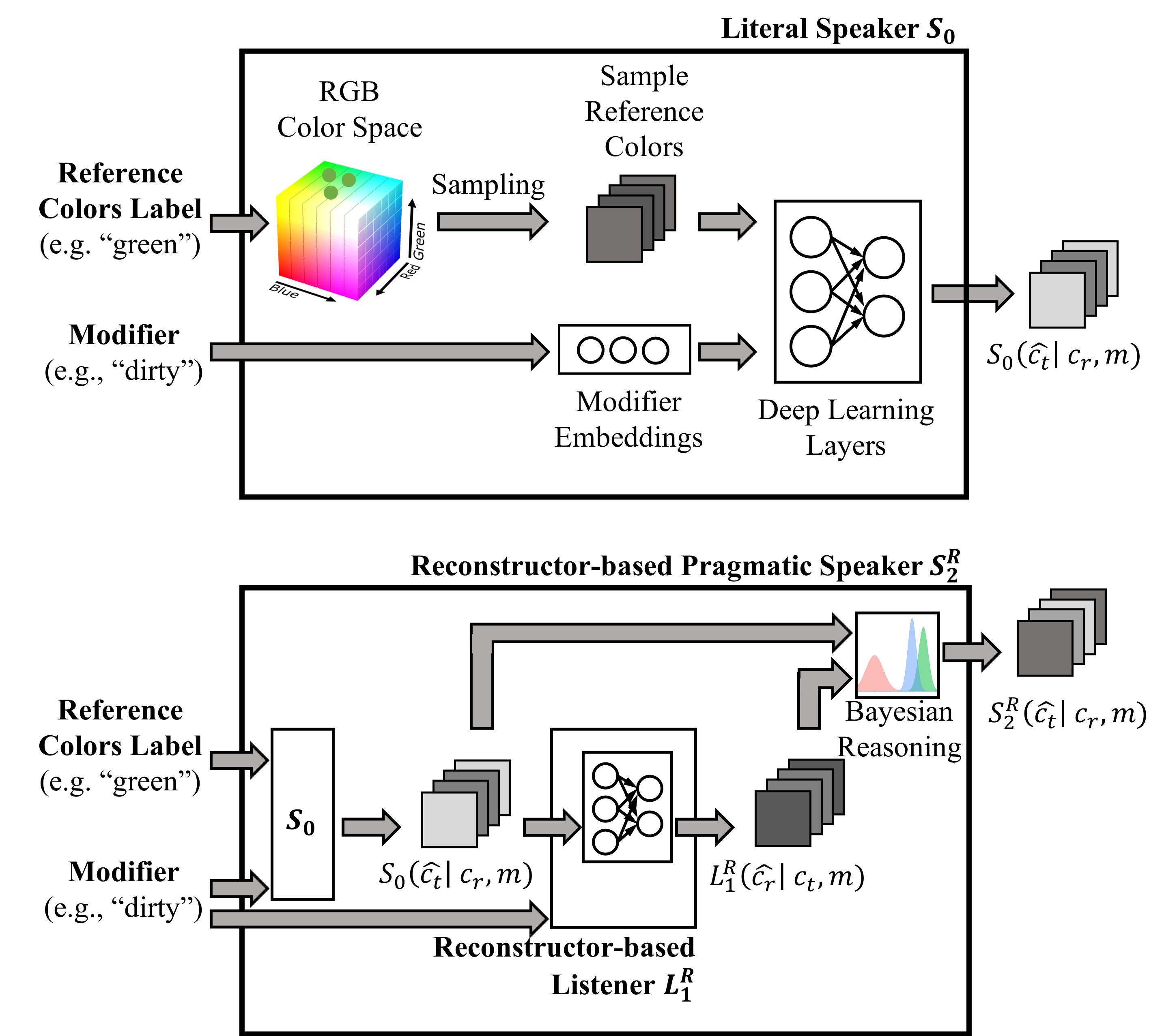
The task is formulated as a conditional color generation task. Given a set of sampled RGB vectors $c_{r}$ for a reference color label and a modifier $m$, our objective is to generate a RGB vector $\hat{c}_{t}$ that is close to the gold-standard RGB vector $c_{t}$ for the target color label. By integrating pragmatic modeling, we focus on generating target colors that are pragmatically informative, i.e., that a potential listener can use to reconstruct the reference colors. This process involves two main steps as shown in Fig. 2. First, a literal speaker model generates and evaluates multiple RGB vectors for a target color given the sampled RGB vectors for a reference color and a modifier. Second, a reconstructor-based pragmatic speaker model “reasons” about an embedded reconstructor-based listener that evaluates the output of the literal speaker model, and thus generates RGB vectors that best allows the listener to reconstruct the reference color RGB vector. We note that the listener is better thought of as a subroutine in the pragmatic speaker model rather than a separate model, and we will discuss it as such.

Literal Speaker

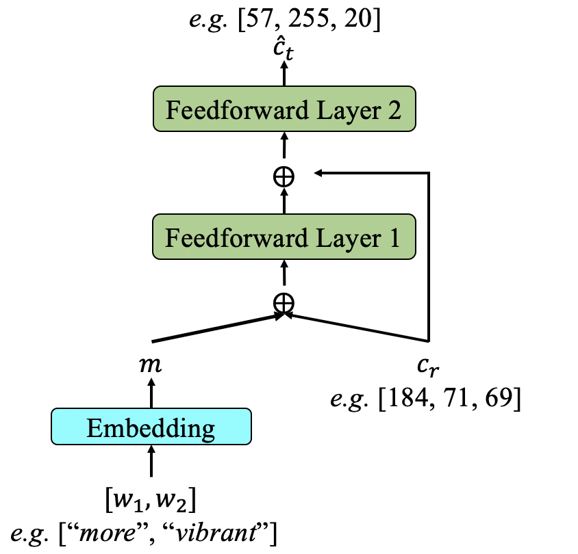
We first describe the base literal speaker model, $S_{0}$, which generates a probability distribution $S_{0}(\hat{c}_{t}|c_{r},m)$ over target colors $\hat{c}_{t}$ given a reference color $c_{r}\in\bm{c_{r}}$ and a modifier $m$ (represented using word embeddings). To parameterize $S_{0}$, we build our literal speaker model using the deep neural network proposed by  Winn and Muresan (2018). The model takes two inputs as shown in Fig. 3: the modifier $m$ and the RGB vector $c_{r}$ for the reference color label. An input modifier is represented by using 300-dimensional GloVe word embeddings Pennington et al. (2014). We represent the modifiers as a bi-gram to account for comparatives that need “more” (e.g. “more vibrant”); single-word modifiers are padded with the zero vector. Both the word embeddings $m$ of modifiers and the color RGB vector $c_{r}$ are concatenated and fed into a fully connected feedforward layer with a hidden size 30:

Figure 3: Model architecture for our base literal speaker $S_{0}$ model, which is based on the model proposed by Winn and Muresan (2018).

$$\begin{split}f_{\phi}(c_{r},m)&=\textbf{W}_{1}[c_{r},m]+\textbf{b}_{1}\end{split}$$ (1)

where $\textbf{W}_{1}$ and $\textbf{b}_{1}$ are learnt parameters. The output hidden state $o_{1}$ of the first layer is concatenated with the color RGB vector, and fed into another fully connected layer $f_{\psi}$ with a hidden size 3 to predict the RGB vector $\hat{c}_{t}$ for a target color label:

$$\begin{split}f_{\psi}(o_{1},m)&=\textbf{W}_{2}[o_{1},c_{r}]+\textbf{b}_{2}\\ \hat{c}_{t}&=f_{\psi}(o_{1},m)\end{split}$$ (2)

where $\textbf{W}_{2}$ and $\textbf{b}_{2}$ are learnt parameters. Following previous works Winn and Muresan (2018), our loss function two parts: (1) minimizing the cosine distance between the “true” color modification in RGB space, $(c_{t}-c_{r})$, and the predicted modification $(\hat{c}_{t}-c_{r})$. (2) minimizing the mean square error between $c_{t}$ and $\hat{c}_{t}$. Intuitively, the first part supervises the model to learn contextual meanings of modifiers, while the second part supervises the model to draw colors accurately.

Test Set	Models
	WM18	HSC19-HSV${}_{\emph{retrain}}$	$S_{0}$	$S_{2}^{R}$
Cosine Similarity (Std. Dev.); Higher = Better
Seen Pairings (SP)	.680 (-)	.869 (.023)	.926 (.002)	.934 (.001)
Unseen Pairings (UP)	.680 (-)	.739 (.115)	.823 (.005)	.834 (.003)
Unseen Ref. Color (URC)	.400 (-)	.424 (.088)	.751 (.007)	.803 (.004)
Unseen Modifier (UM)	.410 (-)	.620 (.132)	.603 (.002)	.690 (.002)
Fully Unseen (FUN)	-.210 (-)	.408 (.099)	.552 (.011)	.564 (.009)
Overall (OR)	.650 (-)	.758 (.056)	.855 (.003)	.859 (.002)
Delta-E Distance (Std. Dev.); Lower = Better
Seen Pairings (SP)	6.10 (-)	5.58 (.022)	5.03 (.012)	4.79 (.011)
Unseen Pairings (UP)	7.90 (-)	8.00 (.082)	5.79 (.008)	5.72 (.006)
Unseen Ref. Color (URC)	11.4 (-)	20.5 (1.33)	10.1 (.011)	9.49 (.013)
Unseen Modifier (UM)	10.5 (-)	16.0 (1.28)	13.2 (.072)	13.2 (.066)
Fully Unseen (FUN)	15.9 (-)	16.4 (.665)	15.0 (.011)	15.0 (.006)
Overall (OR)	6.80 (-)	8.96 (.324)	6.88 (.005)	6.57 (.003)

Table 1: Average cosine similarity score and Delta-E distance over 10 runs, of our literal speaker ($S_{0}$) and our reconstructor-based pragmatic speaker ($S_{2}^{R}$) in comparison to previous models: WM18 proposed by Winn and Muresan (2018), and HSC19-HSV proposed by Han et al. (2019). To facilitate comparison with our models, we retrained HSC19-HSV, with more details in the main text. (-) indicates that standard deviations were not reported in the original paper. Bolded values indicate the best performances.

Previous works that integrate pragmatics into deep learning solve discrimination problems—distinguishing a referent target from similar distractors Andreas and Klein (2016); Monroe et al. (2017); Cohn-Gordon et al. (2018, 2019); Nie et al. (2020). Without the explicit presence of distractors, we use instead samples of $c_{r}\in\bm{c_{r}}$ to serve as distractors. For $\bm{c_{r}}$, we randomly sample $n$ RGB vectors for each color label. We pass each sample through the deep learning layers, to generate multiple target colors. As a result, the model predicts $n$ modified RGB vectors $\hat{c}_{t}\in\bm{\hat{c}_{t}}$ for a target color label. In our experiments, we set $n$ to 10.

To evaluate generated $\hat{c}_{t}$ via sampling, we formulate the probability distribution as $S_{0}(\hat{c}_{t}|c_{r},m)$, by using the distances between RGB vectors in RGB space:

$$\begin{split}S_{0}(\hat{c}_{t}|c_{r},m)&\propto\frac{e^{\Delta(\hat{c}_{t},\bar{\bm{c_{r}}})}}{\sum_{\hat{c}_{t}^{{}^{\prime}}}e^{\Delta(\hat{c}_{t}^{{}^{\prime}},\bar{\bm{c_{r}}})}}\end{split}$$ (3)

where $\bar{\bm{c_{r}}}$ is the mean RGB vector associated with the reference color label. We propose that modified target color is expected to diverge from the reference color in the color space as in Winn and Muresan (2018). We use Delta-E 2000 in CIELAB color space as $\Delta(\cdot)$ in Eqn. 3 and Eqn. 4 (See Sec. 6 for the description and other distance metrics). The RGB vector with the highest probability is considered as the final output for $S_{0}$. We use Delta-E 2000 in CIELAB which is also commonly used in previous works for evaluating model performances in color generation Winn and Muresan (2018) (See Sec. 5 for the definitions). Note that this distance measurements can be replaced by other metrics.

Thus to summarize, our literal speaker model $S_{0}$ takes the base deep learning model proposed by WM18, adds a sampling procedure to produce distractors, and optimizes for target colors that maximize distance in color space. Though adding the sampling procedure is quite intuitive, previous deep learning models suffers from the lack of capability to incorporate the richness of the color representations.

Figure 4: Examples of predictions for our retrained model Han et al. (2019) HSC19-HSV, and our reconstructor-based pragmatic speaker model $S_{2}^{R}$. The Test Sets include: Seen Pairings (SP), Unseen Pairings (UP), Unseen Reference Color (URC), Unseen Modifiers (UM), and Fully Unseen (FUN). For each example, we include reference color (Ref.), predicted modifier, true target color, and results based on our evaluate metrics.

Reconstructor-Based Pragmatic Speaker

To increase informativeness of our outputs from $S_{0}$, we further propose a “listener” that maximizes the probability of reconstructing inputs from the outputs of our literal speaker model. Previous works denote this as a reconstructor-based listener $L_{1}^{R}$ Dušek and Jurcicek (2016); Fried et al. (2018); Shen et al. (2019). The listener produces a probability distribution $L_{1}^{R}(c_{r}|\hat{c}_{t},m)$ by reconstructing $c_{r}$ given a $\hat{c}_{t}$ and $m$. We parameterize $L_{1}^{R}$ using a separate neural network which has the same model architecture as in $S_{0}$ trained with the objective of predicting $c_{r}$ given $c_{t}$ and word embeddings for $m$.

Similar to Equation 3, we formulate the probability distribution for $L_{1}^{R}(c_{r}|\hat{c}_{t},m)$ by considering reconstruction error using the distance between RGB vectors in the RGB space:

$$\begin{split}L_{1}^{R}(c_{r}|\hat{c}_{t},m)&\propto\left(\frac{e^{\Delta(\hat{c}_{r},\bar{\bm{c_{r}}})}}{\sum_{\hat{c}_{r}^{{}^{\prime}}}e^{\Delta(\hat{c}_{r}^{{}^{\prime}},\bar{\bm{c_{r}}})}}\right)^{-1}\end{split}$$ (4)

where $\hat{c}_{r}$ is the reconstructed RGB vector for a reference color label. Unlike Equation 3, we have the probability proportional to the inverse of the distance function as we want the reconstructed reference color to be close to the true reference color.

Now, we introduce our pragmatic model, the reconstructor-based pragamatic speaker model, which combines the literal speaker and the reconstructor-based listener (Fig. 2). This pragmatic speaker model has as “subroutines” that it can call, the literal speaker and the reconstructor-based listener. It “reasons” about the listener, and chooses the most informative colors that the listener can use to reconstruct the original reference colors (which it does by reasoning about the literal speaker). Formally, the reconstructor-based pragmatic speaker generates a probability distribution over $\hat{c}_{t}$, weighting both the $L_{1}^{R}$ and $S_{0}$ terms:

$$\begin{split}S_{2}^{R}(\hat{c}_{t}|c_{r},m)&=L_{1}^{R}(c_{r}|\hat{c}_{t},m)^{\lambda}\cdot S_{0}(\hat{c}_{t}|c_{r},m)^{1-\lambda}\end{split}$$ (5)

where $\lambda$ is a pragmatic reasoning parameter that controls how much the model optimizes for discriminative outputs, following  Monroe et al. (2017). The predicted RGB vector with the highest probability in Eqn. 5 is our pragmatic prediction for $\hat{c}_{t}$. We found an optimal value of $\lambda$ at 0.33 using grid search by evaluating with the Validation set.

5 Experiment Setup

Evaluation:

We evaluate our models under 5 different test sets as in Winn and Muresan (2018); Han et al. (2019): (1) 271 Seen Pairings (SP): The triple (reference color label, modifier, target color label) has been seen in the training set. (2) 29 Unseen Pairings (UP): The reference color label and modifier have been seen in the training set, but not their pairing (i.e., they appeared separately). (3) 63 Unseen Reference Color (URC): reference color label is not present in the training set, but modifier is. (4) 41 Unseen Modifiers (UM): modifier is not present in the training set, but the reference color label is. (5) Fully Unseen (FUN): Neither reference color label or modifier has been seen in the training data. (6) Overall (OR): All samples in the testing set. As mentioned in Sec. 3, we use a different set of RGB vectors in the test sets for a color label that has been seen during training to ensure our model is not overfitting with the training set. We averaged our performance results over 10 runs with distinct random seeds.

We use two different metrics to evaluate our models, following Winn and Muresan (2018); Han et al. (2019): (1) Cosine similarity scores between the two difference vectors $(c_{t}-c_{r})$ and $(\hat{c}_{t}-c_{r})$; Higher scores correspond to better performance. (2) Delta-E distance in CIELAB color space between $c_{t}$ and $\hat{c}_{t}$ (see Winn and Muresan (2018); Han et al. (2019) for discussions). Delta-E is a non-uniformity metric for measuring color differences, which was first presented as the Euclidean Distance in CIELAB color space McLaren (1976).  Luo et al. (2001) present the latest and most accurate CIE color difference metrics, Delta-E 2000, which improves the original formula by taking into account weighting factors and fixing inaccuracies in lightness. Lower Delta-E 2000 values correspond to better performance.

Model configuration:

To train our models, we use a standard laptop with 2.9 GHz Intel Core i7 and 16 GB 2133 MHz LPDDR3 with GPU training disabled. With this computing infrastructure, it takes about 10 minutes to train all of our models, where each model is trained with 500 epochs. Our literal speaker model $S_{0}$ contains 18,222 trainable parameters which is the same as reconstructor-based listener model $L_{1}^{R}$. Our reconstructor-based listener pragmatic speaker $S_{2}^{R}$ contains 36,445 trainable parameters.

6 Results

Table 1 shows test results, in comparison with previous best performing models. We retrain the best performing model HSC19-HSV Han et al. (2019) with our evaluation pipeline to ensure fairness.

Compared to the both models, our literal model $S_{0}$ achieves better performance across most test cases while maintains similar performance in others as shown in the Table 1. This is expected given the fact that $S_{0}$ maximizes information gain via additional evaluating with sampling procedure. Our pragmatic model $S_{2}^{R}$ further increases performances across all Test sets by outperforming our literal model $S_{0}$ with significant gains, which is expected given the model adds pragmatic informativeness. For all the test sets, $S_{2}^{R}$ exceeds the state-of-the-art (SOTA) deep learning based models across both evaluation metrics. For more difficult test cases where one of the input is unseen, our models perform extremely well. For instance, our $S_{2}^{R}$ model has a 95% absolute increase in cosine similarity score for the Unseen Reference Color (URC) test set. For the Fully Unseen (FUN) test set where both the reference color and the modifier are unseen during training, our $S_{2}^{R}$ still shows the ability to generalize to new test samples with a 40% increase in cosine similarity score comparing to previous models who perform poorly with unseen data.

The performance gain from our pragmatic models suggests that contextual descriptions of colors might be pragmatically generated by participants. For example, when participants are asked to describe a color  , previous studies have found people rely on using adjective modifiers (e.g., “dirty”) with a reference to a base color (e.g., “green”) Lassiter and Goodman (2017). The pragmatic approach offers an additional step: when participants are selecting a base color implicitly, they may also be de-modifying the color showed to them.

Error Analysis:

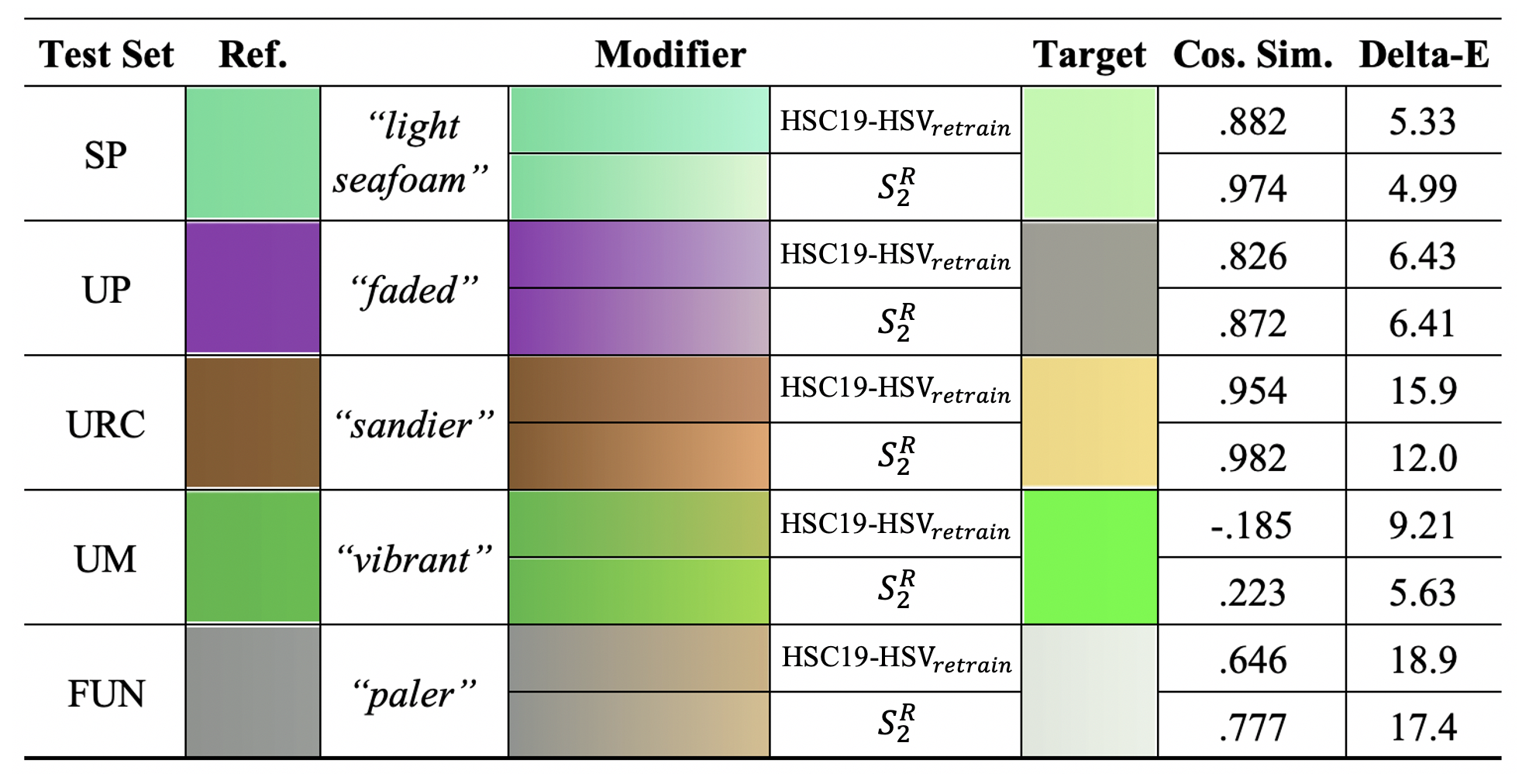
In Fig. 4, we provide selected illustrative examples from each of the five Test sets. We discuss the two cases from the UM and FUN test sets. For the UM example, the reference color is “green” and the modifier is “vibrant”. Since in our training, the word embedding for “vibrant” is unseen, the non-pragmatic (literal) model results in a negative cosine similarity.

On the other hand, our pragmatic model $S_{2}^{R}$ is capable of making more accurate predictions when presented with previously unseen test cases. This is expected as, by performing additional recursive evaluation, the pragmatic model is able to choose more “informative” target colors. This is consistent across all Test sets where we have unseen test examples. For FUN test set, both $S_{0}$ and $S_{2}^{R}$ models make poor predictions. We expect that for unseen modifiers, the predictions should be based on modifiers with similar meanings. For example, “paler” should be similar to some seen modifiers, e.g. “whiten”, “faded”. However, the predicted modification is more close to “sandier” in this case. As described in Mrkšić et al. (2016), this may related to closeness in the word embedding space for these modifiers.

Figure 5: Test result for each Test set evaluated by cosine similarity with different distance-based probability estimations over 10 runs. Error bars represents standard deviation of the cosine similarity.

Figure 6: Test result for each Test set evaluated by Delta-E 2000 distance Luo et al. (2001) in CIELAB color space McLaren (1976) with different distance-based probability estimations over 10 runs. Error bars represents standard deviation of the Delta-E 2000 distance.

Distance Metrics:

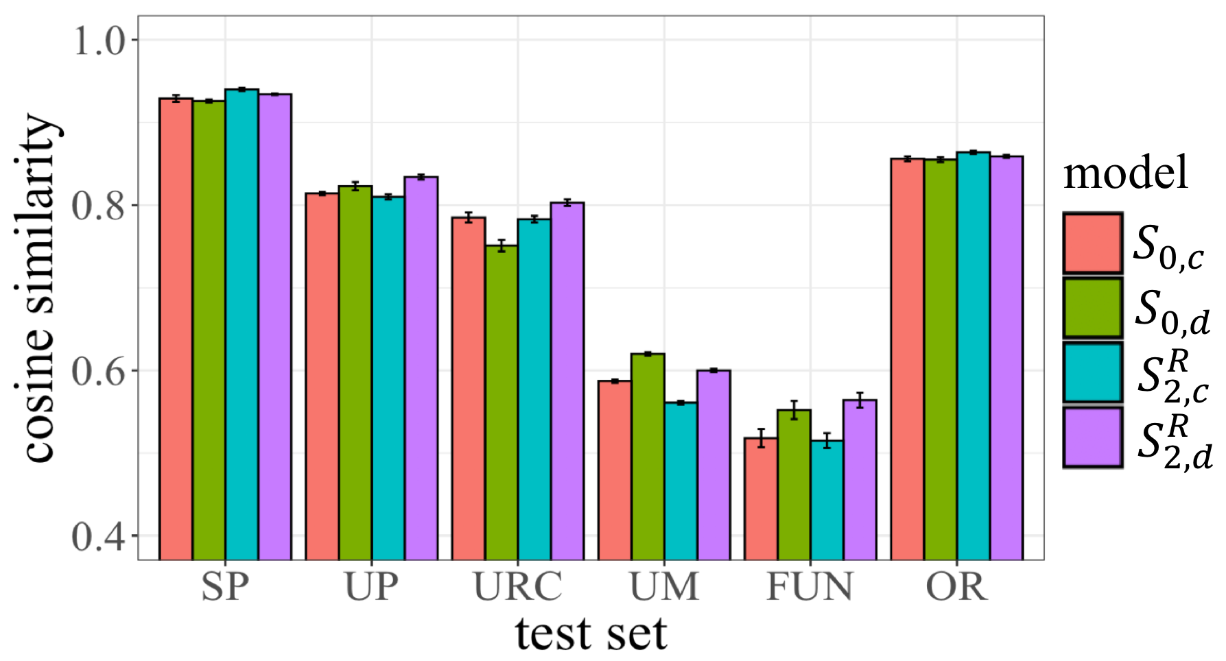
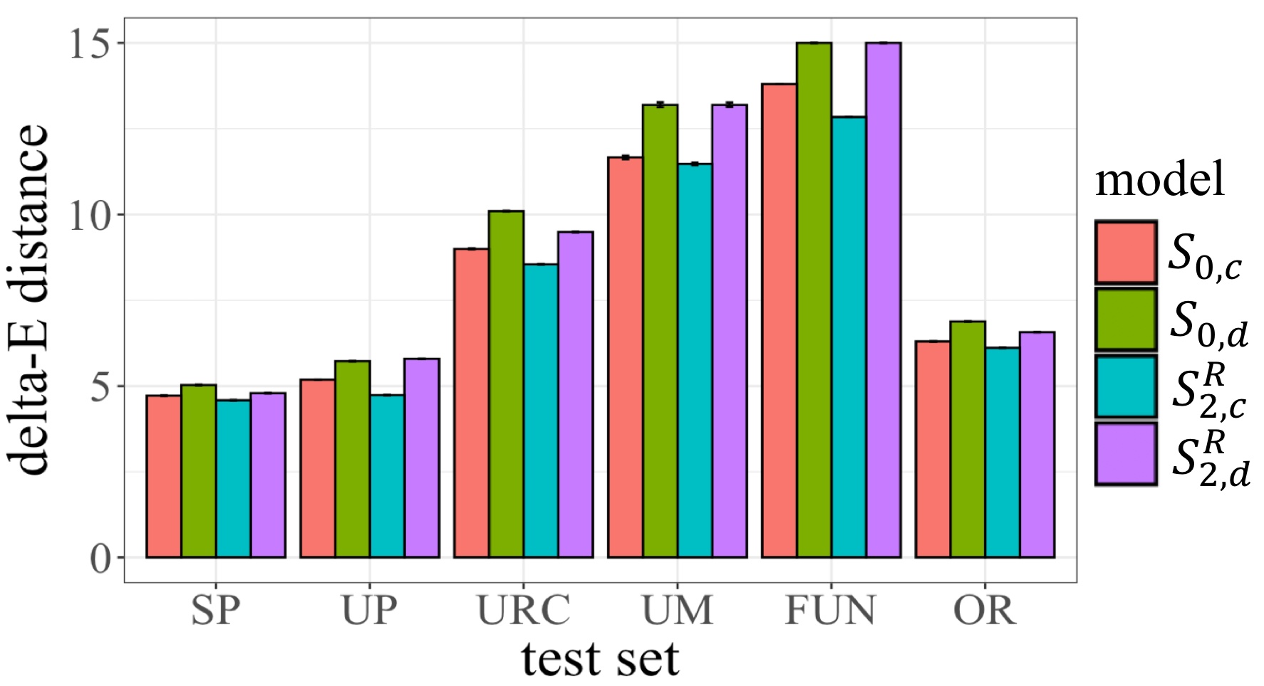
As mentioned, we use Delta-E 2000 distance in the CIELAB color space as $\Delta(\cdot)$ in Eqn. 3 and Eqn. 4 by default. Additionally, we use cosine distance in the RGB color space as our distance metrics to formulate our distance-based probability estimations. We denote $S_{0,\text{c}}$ and $S_{2,c}^{R}$ for cosine distance based estimation, and $S_{0,d}$ and $S_{2,d}^{R}$ for Delta-E 2000 based estimation. Results are shown in Fig. 5 and Fig. 6. Our result suggests that Delta-E 2000 based models perform better in most of test cases. This result corroborates with previous works suggesting Delta-E 2000 based distance in CIELAB color space is more accurate in describing nuanced difference between colors Luo et al. (2001). As shown in Fig. 5 and Fig. 6, reconstructor-based pragmatic speaker models are consistently outperforming literal speaker models across multiple Test sets.

7 Conclusion and Future Work

In this paper, we propose a novel reconstructor-based pragmatic speaker model, and apply it to a color generation task that requires extensive grounding of contextual modifiers in color space. Our base literal speaker model, with no pragmatics and which adapts previous deep learning models with distractor sampling, performs respectably on modifiers and colors that it was trained on, but performs poorly when testing on previously unseen modifiers and colors. Our pragmatic speaker model reasons about a listener that tries to guess the speaker’s input, and hence provides pragmatically informative utterances (colors). The output of the pragmatic speaker model shows consistent improvements in performance over the base literal speaker model across multiple testing conditions, unseen test words (e.g. unseen colors). We note that in this case (and in many other datasets as well), the data was generated by people—perhaps people may be applying some pragmatic reasoning when labeling colors. We speculate that this might both (i) explain the performance of the pragmatic speaker model, and (ii) justify the pragmatic assumptions we make in building our model. This hypothesis would need to be further confirmed with additional human experiments, but overall we are hopeful that this bodes well for this general endeavour of augmenting deep learning approaches with pragmatics to build better models of natural language understanding.

Our pragmatic pipeline provides another successful example of applying pragmatic modelings in traditional machine learning generation tasks, and the first to do so with a simple “image” (color) output. Future work could explore merging this approach with deep learning methods in other more complex contextual image generation tasks, such as generating images from natural language captions.

References

- Andreas and Klein (2016) Jacob Andreas and Dan Klein. 2016. Reasoning about pragmatics with neural listeners and speakers. In Proceedings of the 2016 Conference on Empirical Methods in Natural Language Processing, pages 1173–1182.
- Cohn-Gordon et al. (2018) Reuben Cohn-Gordon, Noah Goodman, and Christopher Potts. 2018. Pragmatically informative image captioning with character-level inference. In Proceedings of the 2018 Conference of the North American Chapter of the Association for Computational Linguistics: Human Language Technologies, Volume 2 (Short Papers), pages 439–443.
- Cohn-Gordon et al. (2019) Reuben Cohn-Gordon, Noah Goodman, and Christopher Potts. 2019. An incremental iterated response model of pragmatics. In Proceedings of the Society for Computation in Linguistics (SCiL) 2019, pages 81–90.
- Dušek and Jurcicek (2016) Ondřej Dušek and Filip Jurcicek. 2016. Sequence-to-sequence generation for spoken dialogue via deep syntax trees and strings. In Proceedings of the 54th Annual Meeting of the Association for Computational Linguistics (Volume 2: Short Papers), pages 45–51.
- Egré et al. (2013) Paul Egré, Vincent de Gardelle, and David Ripley. 2013. Vagueness and order effects in color categorization. Journal of Logic, Language and Information, 22(4):391–420.
- Farhadi et al. (2009) Ali Farhadi, Ian Endres, Derek Hoiem, and David Forsyth. 2009. Describing objects by their attributes. In 2009 IEEE Conference on Computer Vision and Pattern Recognition, pages 1778–1785. IEEE.
- Frank and Goodman (2012) Michael C Frank and Noah D Goodman. 2012. Predicting pragmatic reasoning in language games. Science, 336(6084):998–998.
- Fried et al. (2018) Daniel Fried, Jacob Andreas, and Dan Klein. 2018. Unified pragmatic models for generating and following instructions. In Proceedings of the 2018 Conference of the North American Chapter of the Association for Computational Linguistics: Human Language Technologies, Volume 1 (Long Papers), pages 1951–1963.
- Goodman and Stuhlmüller (2013) Noah D Goodman and Andreas Stuhlmüller. 2013. Knowledge and implicature: Modeling language understanding as social cognition. Topics in cognitive science, 5(1):173–184.
- Han et al. (2019) Xudong Han, Philip Schulz, and Trevor Cohn. 2019. Grounding learning of modifier dynamics: An application to color naming. In Proceedings of the 2019 Conference on Empirical Methods in Natural Language Processing and the 9th International Joint Conference on Natural Language Processing (EMNLP-IJCNLP), pages 1488–1493.
- Lassiter and Goodman (2017) Daniel Lassiter and Noah D Goodman. 2017. Adjectival vagueness in a bayesian model of interpretation. Synthese, 194(10):3801–3836.
- Luo et al. (2001) M Ronnier Luo, Guihua Cui, and Bryan Rigg. 2001. The development of the cie 2000 colour-difference formula: Ciede2000. Color Research & Application: Endorsed by Inter-Society Color Council, The Colour Group (Great Britain), Canadian Society for Color, Color Science Association of Japan, Dutch Society for the Study of Color, The Swedish Colour Centre Foundation, Colour Society of Australia, Centre Français de la Couleur, 26(5):340–350.
- McLaren (1976) K McLaren. 1976. Xiii—the development of the cie 1976 (l* a* b*) uniform colour space and colour-difference formula. Journal of the Society of Dyers and Colourists, 92(9):338–341.
- McMahan and Stone (2015) Brian McMahan and Matthew Stone. 2015. A Bayesian model of grounded color semantics. Transactions of the Association for Computational Linguistics, 3:103–115.
- Monroe et al. (2017) Will Monroe, Robert XD Hawkins, Noah D Goodman, and Christopher Potts. 2017. Colors in context: A pragmatic neural model for grounded language understanding. Transactions of the Association for Computational Linguistics, 5:325–338.
- Mrkšić et al. (2016) Nikola Mrkšić, Diarmuid Ó Séaghdha, Blaise Thomson, Milica Gasic, Lina M Rojas Barahona, Pei-Hao Su, David Vandyke, Tsung-Hsien Wen, and Steve Young. 2016. Counter-fitting word vectors to linguistic constraints. In Proceedings of the 2016 Conference of the North American Chapter of the Association for Computational Linguistics: Human Language Technologies, pages 142–148.
- Munroe (2010) Randall Munroe. 2010. Color survey results. Online at http://blog.xkcd.com/2010/05/03/color-survey-results.
- Nie et al. (2020) Allen Nie, Reuben Cohn-Gordon, and Christopher Potts. 2020. Pragmatic issue-sensitive image captioning. arXiv preprint arXiv:2004.14451.
- Pennington et al. (2014) Jeffrey Pennington, Richard Socher, and Christopher D Manning. 2014. Glove: Global vectors for word representation. In Proceedings of the 2014 conference on empirical methods in natural language processing (EMNLP), pages 1532–1543.
- Russakovsky and Fei-Fei (2010) Olga Russakovsky and Li Fei-Fei. 2010. Attribute learning in large-scale datasets. In European Conference on Computer Vision, pages 1–14. Springer.
- Shen et al. (2019) Sheng Shen, Daniel Fried, Jacob Andreas, and Dan Klein. 2019. Pragmatically informative text generation. In Proceedings of the 2019 Conference of the North American Chapter of the Association for Computational Linguistics: Human Language Technologies, Volume 1 (Long and Short Papers), pages 4060–4067.
- Vedaldi et al. (2014) Andrea Vedaldi, Siddharth Mahendran, Stavros Tsogkas, Subhransu Maji, Ross Girshick, Juho Kannala, Esa Rahtu, Iasonas Kokkinos, Matthew B Blaschko, David Weiss, et al. 2014. Understanding objects in detail with fine-grained attributes. In Proceedings of the IEEE conference on computer vision and pattern recognition, pages 3622–3629.
- Winn and Muresan (2018) Olivia Winn and Smaranda Muresan. 2018. ‘lighter’can still be dark: Modeling comparative color descriptions. In Proceedings of the 56th Annual Meeting of the Association for Computational Linguistics (Volume 2: Short Papers), pages 790–795.