Refining Semantic Segmentation with Superpixels using
Transparent
Initialization and Sparse Encoder
Abstract
Although deep learning greatly improves the performance of semantic segmentation, its success mainly lies in object central areas without accurate edges. As superpixels are a popular and effective auxiliary to preserve object edges, in this paper, we jointly learn semantic segmentation with trainable superpixels. We achieve it with fully-connected layers with Transparent Initialization (TI) and efficient logit consistency using a sparse encoder. The proposed TI preserves the effects of learned parameters of pretrained networks. This avoids a significant increase of the loss of pretrained networks, which otherwise may be caused by inappropriate parameter initialization of the additional layers. Meanwhile, consistent pixel labels in each superpixel are guaranteed by logit consistency. The sparse encoder with sparse matrix operations substantially reduces both the memory requirement and the computational complexity. We demonstrated the superiority of TI over other parameter initialization methods and tested its numerical stability. The effectiveness of our proposal was validated on PASCAL VOC 2012, ADE20K, and PASCAL Context showing enhanced semantic segmentation edges. With quantitative evaluations on segmentation edges using performance ratio and F-measure, our method outperforms the state-of-the-art.
![[Uncaptioned image]](/html/2010.04363/assets/figures/sota.jpg)
1 Introduction
Semantic segmentation is an essential task in computer vision which requires mapping image pixels of interesting objects to predefined semantic labels. Applications include autonomous driving [14], object identification [36, 38], image editing [22], and scene analysis [21]. Recent developments of semantic segmentation are greatly promoted by deep learning on several large-scale datasets [35, 32], resulting in effective networks [34, 55, 58, 8, 7, 9, 53, 54]. Semantic segmentation obtained by these methods, however, is not substantially aligned with object edges.
This problem can be alleviated by using qualified edge-preserving methods [28, 58, 8] or independently learning edges for semantic segmentation [25, 17, 7]. Nevertheless, those edges are usually incomplete and oversegmented. To solve this problem, denseCRF [28] based methods aggregate object features over a large and dense range using bilateral filters with high-dimensional lattice computations. This, however, could be more efficient and desirable to learn on locally oversegmented areas, such as superpixels that aggregate similar pixels into a higher-order clique [1, 30].
Existing superpixel segmentation approaches are mainly categorized into traditional methods, such as SLIC [1], LSC [30], Crisp [24], BASS [47], and those using neural networks, such as SSN [25], affinity loss [46], and superpixels by FCN [52]. Although those traditional methods have qualified performance on superpixel segmentation, they cannot be easily embedded into neural networks for end-to-end learning due to nondifferentiability or large computational complexity. In contrast, [25] provides an end-to-end learning for superpixel semantic segmentation, but the pixel labels in each superpixel are not always consistent. Similarly, [52] uses a fully convolutional network to learn superpixels for stereo matching, which is the current state-of-the-art in superpixel learning. However, the problem of inconsistent pixel labels in each superpixel will also occur when [52] is applied to semantic segmentation.
To deal with the problems of edge loss and inconsistent superpixel labelling, we jointly train these networks with additional fully-connected layers using transparent initialization and logit consistency, resulting in enhanced object edges in Fig. 1. Specifically, transparent initialization warm starts the training by recovering the pretrained network output from its input at initialization, followed by a gradual improvement in learning superpixels. Simultaneously, logit consistency with sparse encoder enables efficient logit averaging to guarantee consistent pixel labels in each superpixel. Furthermore, we used the popular performance ratio [27] and F-measure [42, 15] to evaluate the quality of semantic segmentation edges. Our code will be available upon publication. The main contributions of this work are:
-
•
We jointly learn the state-of-the-art semantic segmentation network and superpixel network to enhance the labelling performance with sharp object edges. The improvement is vivid as demonstrated by evaluating on PASCAL VOC 2012, ADE20K and PASCAL Context.
-
•
Transparent initialization is proposed for learning fused features while adding fully-connected layers to pretrained networks. This helps to join and fine-tune state-of-the-art networks without interrupting the effect of pretrained network parameters. The transparent initialization may also be adapted to fine-tune multiple and deeper pretrained networks for other tasks.
-
•
Logit consistency, implemented by a sparse encoder with sparse matrix operations, ensures consistent semantics for all pixels in each superpixel. This makes it feasible and efficient to index pixels by superpixels, because of greatly reduced computational complexity.
2 Related Work
Semantic Segmentation.
Semantic segmentation can be traced back to early techniques [45] based on classifiers, such as random decision forests [39], SVMs [49], and graphic models with MRFs and CRFs [26, 28, 3]. In contrast, modern state-of-the-art methods rely on advanced exploitation of deep CNN classifiers, such as ResNet [20], DenseNet [23], and VGG16 [41]. Fully Convolutional Network (FCN) [34] and related methods are typical architectures that use rich image features from classifiers usually pretrained on ImageNet [12]. SegNet [5] uses a U-Net structure for an encoder-decoder module to compensate for low resolution by using multiple upsampled feature maps. In addition, several multiscale contextual fusion methods [7, 31, 9] have been proposed to aggregate pyramid feature maps for fine-grained segmentation. Typically, DeepLabV3+ [9] combines spatial pyramid pooling and encoder-decoder modules to refine the segmentation along with object boundaries. Recently, attention-based networks [29, 56, 11, 16] improve object labelling confidence by aggregating features of a single pixel with those from other positions. Zhang et al. [54] introduce a split-attention block in ResNet (ResNeSt), which enables multiscale scores with softmax for attention across feature-map groups. This achieves the new state-of-the-art performance in semantic segmentation and image classification. Due to the limited capability of network architectures, however, a huge improvement on mean Intersection over Union (mIoU) is hard to achieve; see the minor improvement in [57].
Superpixel Segmentation.
Superpixel segmentation has been well studied for years with a comprehensive survey in [43]. In contrast to classical methods that initialize superpixel regions with seeds and cluster pixel sets using distance measurement [48], boundary pixel exchange [6], etc., the widely-used SLIC based methods [1, 33, 30, 2] employ (weighted) K-means clustering on pixel feature vectors to group neighbouring pixels. In deep learning, SSN [25] first proposes an end-to-end learning framework for superpixels with differentiable SLIC for semantic segmentation and optical flow. By comparison, [52] replaces the soft K-means manner in SSN with a simple fully convolutional network and applies it to stereo matching with downsampling and upsampling modules. While SSN results in superpixel-level semantic segmentation, the pixel labelling is not aligned with the superpixels. For instance, inconsistent labels exist in each superpixel, which reduces the effects of superpixels on semantic assignments.
Superpixel Semantic Segmentation.
Some works use superpixels to optimize graph relations [19, 50] or downsample images as a pooling alternative to max or average pooling [17, 37, 40]. These methods usually use fixed superpixels obtained by traditional methods mentioned above (“Superpixel Segmentation”) and lose the exact alignment of segmentation edges with superpixel contours after upsampling. This, however, can be easily achieved by our logit consistency module. Moreover, fixed superpixels are unsuitable for end-to-end learning since traditional methods, such as SLIC [1], are computationally expensive due to CPU execution and inflexible for fine-tuning superpixels around object edges, especially for small objects. Instead, superpixels learned by CNN alleviate this problem.
3 Methodology
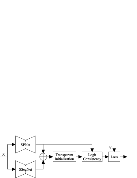
The flowchart of our method is shown in Fig. 2. Subsequently, we discuss each of these modules in detail.
3.1 Network Architectures
We use the state-of-the-art DeepLabV3+ [9] and ResNeSt [54] for semantic segmentation and the state-of-the-art superpixels with FCN [52] for superpixel contours.
DeepLabV3+ achieves high and robust performance with atrous spatial pyramid pooling for multiscale feature maps and encoder-decoder modules for deep features with different output strides. It is widely used as a network backbone for semantic segmentation due to these well-studied modules evaluated by empirical experiments. ResNeSt [54] replaces ResNet with multiscale scores using softmax-based feature map attention and achieves the new state-of-the-art. The loss function for semantic segmentation is the standard cross-entropy loss of predicted logits and ground truth labelling. Readers can refer [9, 54] for more details.
Superpixel with FCN [52] is the current state-of-the-art superpixel network. The core idea is to construct a distance-based loss function with aggregations of neighbouring pixel and superpixel properties and locations. This is similar to the SLIC method [1], where the property vectors can be CIELAB colors or one-hot semantic encoding. The loss function for superpixel network with FCN [52] is in Eq. (1).
Given an image with pixels and superpixels, we denote the subsets of pixels as , where is a subset of pixels belonging to superpixel . With pixel property ( features for each pixel) and probability map , the loss function is
| (1) |
with
| (2a) | ||||
| (2b) | ||||
where is a weight balancing the effects of property and coordinates on loss, is a superpixel sampling interval in proportion to superpixel size, for all are pixel coordinates, is a distance measure function involving norm or cross-entropy, is the probability of pixel belonging to superpixel , and is a set of superpixels surrounding pixel .
Here, and are superpixel-level property vector and central coordinates aggregated from involved pixels respectively, and and are pixel-level property and coordinates aggregated from surrounding superpixels. This updates between pixels and superpixels until the loss converges.

3.2 Learning with Transparent Initialization
Although some semantic segmentation datasets, such as PASCAL VOC [13] and Berkeley benchmark [35], have no accurate edges for supervised edge learning, it can be compensated for by a superpixel network on edge-specified datasets, such as SBDS500 [4]. Due to the domain gap of datasets, however, pretrained superpixel models are more desirable than learning from scratch for fast loss convergence. Superpixel maps pretrained on BSDS500, however, are not always suitable for semantic segmentation datasets. Hence, fine-tuning by joint learning is necessary to improve the quality of superpixel contours, compared with using the pretrained network, as shown in Fig. 3.
Therefore, in our proposal, linear layers or convolutional layers with kernels are added to fuse the outputs of superpixel and semantic segmentation networks. Either or both can be pretrained. Importantly, selecting an appropriate initialization on these additional layers is important to avoid overriding the effect of learned network parameters. It is straightforward to cast the layer operations as an identity mapping between input and output at the early training stage. Net2Net [10] achieves this by using identity matrices to initialize linear layers. This method, however, is inefficient in learning since the identity matrices will result in highly sparse gradients. In addition, it cannot handle activation functions with negative values.
In contrast, we introduce transparent initialization with non-zero values for dense gradients, while identically mapping the layer input to output and preserving the effect of the learned parameters of the pretrained networks.
Affine Layers.
A linear layer without activation (such as a convolution or fully-connected layer) can be written as with layer weights , bias , and input , by matrix multiplication with :
| (3) |
For simplicity the mapping Eq. (3) will be denoted as where denotes the affine transformation, and we place the functions on the right. Note the difference between , an affine transform and , a matrix. If an activation function is included, then the mapping is .
The right-inverse of an affine transformation Eq. (3) is represented by the matrix
| (4) |
satisfying , the identity map. Here, is the right-inverse of matrix , which exists if A has dimension and rank , in which case .
Transparent Initialization.
The idea behind transparent layer initialization is to construct a sequence of affine layers denoted such that is a right-inverse of the product , satisfying , the identity transformation.
A necessary condition for this right inverse to exist is that should be of full rank. Since a matrix with random entries will almost surely have full rank, this leads to the following condition.
Theorem 1
Let a sequence of affine transformations , for be chosen at random. Then almost surely has a right inverse if and only if for .
Therefore, the strategy for selecting a set of parameters for a sequence of affine layers may be described as follows. For the sequence of layers to represent an identity transform, we need that the input and output space have the same dimension, namely . Then
-
1.
Select intermediate dimensions such that for all .
-
2.
Define random affine transforms by selecting the entries of matrices and vectors randomly, using a suitable random number generator, for instance by a zero-mean normal (Gaussian) distribution.
-
3.
Compute the composition by matrix multiplication, and take its right-inverse.
-
4.
Set to equal .
The resulting composite mapping is the identity affine transformation.

With Activation.
Usually, each affine mapping will be followed by an activation function . For now, we assume that this is ReLU(). Our approach including activations is to apply the activation to both and and then sum them. Consider
| (5) |
where mappings (duplicate) and (subtract) are the mappings as shown above, and and are the positive and negative components of . This shows that , and so is the identity mapping. Note also that both and are affine (in fact linear) transformations.
Applying this to a sequence of affine transformations such that gives
| (6) |
Bracketing this differently gives
| (7) |
where now each bracket is an affine mapping followed by the activation (except the last). This may then be implemented as a sequence of affine layers (convolution or fully-connected) with activations. Thus, is the mapping
| (8) |
The mapping is the affine transformation
| (9) |
and is the mapping
| (10) |
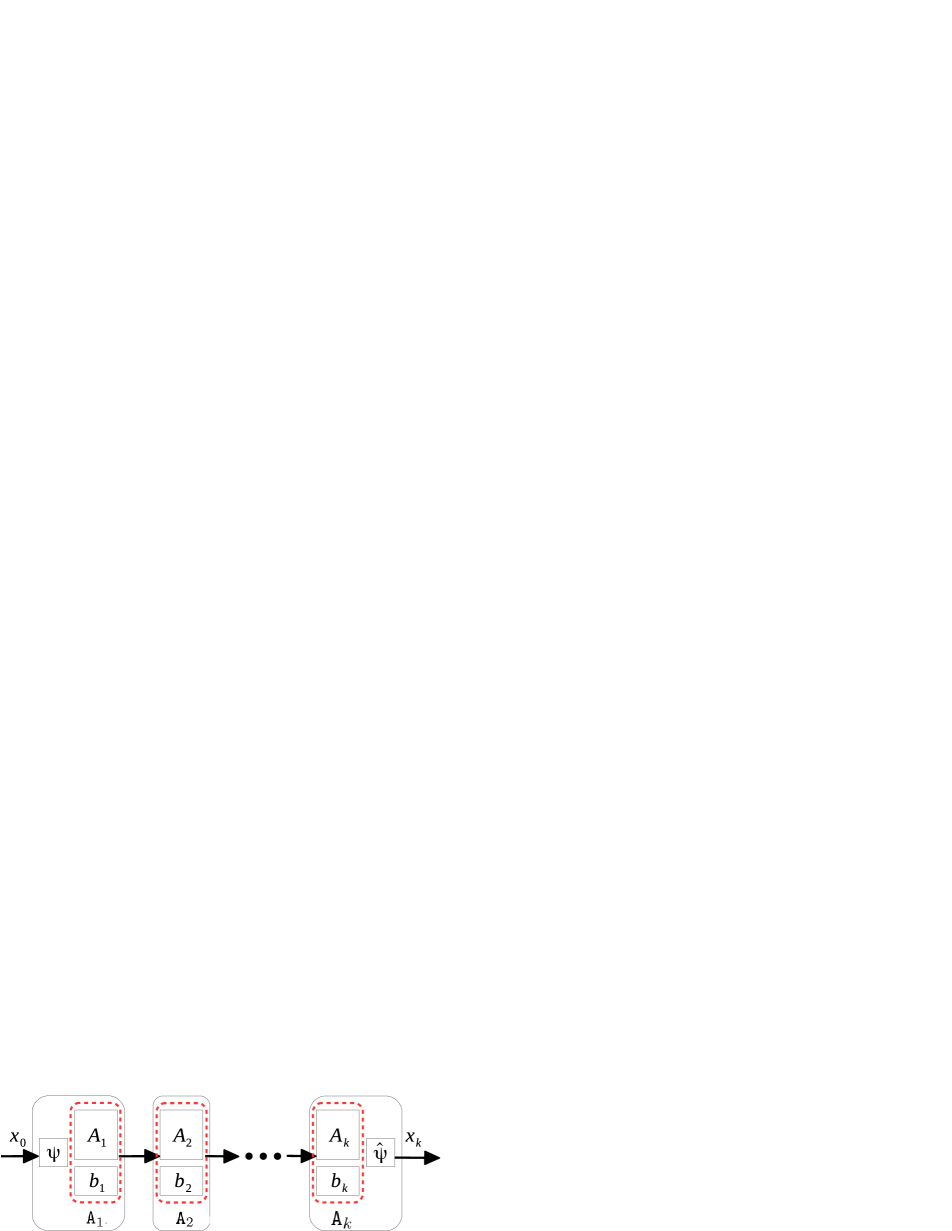
The structure of the network may be represented as in Fig. 4. Observe that the outputs of intermediate layers have twice the dimension of the output of the affine mappings .
It is important to note that the structured form of the affine mappings in Eqs. (8)-(9) are for initialization only. There is no sharing parameters (such as and ) and layers are free to implement any affine transform during training. In fact, in any activation functions satisfying
| (11) |
where is a non-zero constant, can be recovered, such as SoftReLU() defined by and LeakyReLU() [51]:
| (12) |
where is the slope of the negative part of LeakyReLU(). The substitution of Eq. (12) to Eqs. (8)-(9) contributes to the identity mapping in our transparent initialization. One can derive it in a similar way to ReLU(). More details are given in the supplementary material.
3.3 Logit Consistency with Sparse Encoder
| pixel index | ||||||||
| 0 | 1 | 2 | 3 | 4 | -1 | |||
| superpixel index |
0 |
0 | 1 | 1 | 0 | 0 | 0 | |
|
1 |
0 | 0 | 0 | 1 | 1 | 0 | ||
|
2 |
1 | 0 | 0 | 0 | 0 | 1 | ||
|
-1 |
0 | 0 | 0 | 0 | 0 | 0 | ||
| sum | 1 | 1 | 1 | 1 | 1 | 1 | ||
In addition to the notations of pixel number , superpixel number , and subsets of pixels in Sec. 3.1, the label set is defined as given labels. For logit of for superpixel at label , the logit consistency follows
| (13) |
which guarantees all pixels in having the same logit at each label so as to be assigned with the same label.
Nevertheless, considering the high complexity of indexing , a dense matrix operation requires a large GPU memory, that is , especially for the back-propagation in CNN learning. This makes it infeasible for training due to the limited GPU memory in our experiments.
Hence, we adopted a sparse encoder, including sparse encoding and decoding, with sparse matrix operations for the consistency. Let us set matrix for indexing pixels by superpixels as , logit matrix as , where , , and , sparse encoding and decoding are
| (14a) | ||||
| (14b) | ||||
where is {0, 1} binary, shown in Table 1, SMM() is sparse matrix multiplication, and SADD() is sparse addition. This converts Eq. (13) from dense operations to sparse with reduced complexity from to . Otherwise, it is infeasible to jointly train the networks due to the limited GPU memory in our experiments.
4 Experiments
We first evaluated the properties of our transparent initialization including its effectiveness of data recovery and numerical stability. Then, we demonstrated its effect on jointly learning pretrained networks of semantic segmentation and superpixels together with a sparse encoder for logit consistency. Our code in PyTorch will be released on GitHub upon publication.
4.1 Properties of Transparent Initialization
Effectiveness.
Our transparent initialization aims at identically mapping the output of linear layer(s) to the input at the early stage when fine-tuning pretrained network(s). It retains the effect of learned parameters of pretrained model(s). Off-the-shelf parameter initialization methods, such as random (uniform) and Xavier [18] initialization, lead to random values of the output at the early training stage, which cannot generate effective features by the pretrained models. Also, compared with the identical initialization with identity matrices for deeper networks in Net2Net [10], our transparent initialization has a high initialization rate with much more non-zero parameters for dense gradients in the backpropagation.
We evaluated these methods on 3 fully-connected layers. The (in_channels, out_channels) for each layer is (42, 64)(64, 64)(64, 42). Since Net2Net only supports square linear layer, i.e., in_channels equals out_channels, to increase network depth, all layers have 42 in_channels and out_channels. Input data is normally distributed with size (4, 42, 512, 512) as (batch, in_channels, height, width).
In Table 2, random and Xavier initialization have 98% initialization rate but cannot recover the output from its input, leading to 0% recovery rate. Net2Net [10] has only 2% initialization rate and 50% recovery rate with ReLU() for non-negative values only. In contrast, our transparent initialization has a high initialization rate and 100% recovery rate by Eqs. (8)-(10) with ReLU().
Numerical Stability.
Since the effect of our transparent initialization is distributed across layers and Eq. (4) is achieved by a pseudo-inverse matrix for a rank-deficient matrix, hidden layers have round-off errors, and thus, the matrix multiplication of layer parameters is not strictly identical. We therefore tested the numerical stability of our transparent initialization on 4 numerical orders in Table 3. Clearly, the max error between input and output is in proportion to the magnitude of input values. For a pretrained model, its output is usually stable in a numerical range, such as probability in [0, 1]. One can easily enforce a numerical regularization if the model output is out of range.
| Manner | Init. Rate | Recovery Rate | Non-square Filter Supported | |
| w/o Activation | w Activation | |||
| Random | 98.2 | 0.0 | 0.0 | ✓ |
| Xavier [18] | 98.2 | 0.0 | 0.0 | ✓ |
| Net2Net [10] | 2.3 | 100.0 | 50.0 | ✗ |
| Ours | 99.9 | 100.0 | 100.0 | ✓ |
| [-1, 1] | [-10, 10] | [-1e2, 1e2] | [-1e3, 1e3] | |
| Max Error | 6.8e-6 | 6.6e-5 | 6.5e-4 | 6.6e-3 |
4.2 Implementation Setup
Datasets.
We evaluated our proposal on 3 popular semantic segmentation datasets, ADE20K, PASCAL VOC 2012, and PASCAL Context. ADE20K [59, 60] has 150 semantic categories for indoor and outdoor objects. It contains 20,210 samples for training and 2,000 samples for validation. PASCAL Context [36] has additional annotations for PASCAL VOC 2010 and provides annotations for the whole scene with 400+ classes. We selected the given 59 categories for semantic segmentation with 4,996 training samples and 5,104 validation samples. PASCAL VOC 2012 [13] and Berkeley benchmark [35] were used as a combined version for 21 classes segmentation. This dataset has 1,449 images from PASCAL VOC 2012 val set for validation and 10,582 images for training. Meanwhile, MS-COCO [32] was used to pretrain the semantic segmentation network, i.e., DeepLabV3+ in our case, for PASCAL VOC 2012. It has 92,516 images for training and 3,899 images for validation, while 20 object classes from the primary 80 classes were selected in accordance with PASCAL VOC 2012.
Learning Details.
For the ablation study on PASCAL VOC 2012, we trained DeepLabV3+ from scratch on the combined dataset above with crop size . We set Learning Rate (LR) as 0.007 for ResNet and 0.07 for ASPP and decoder. To train on MS-COCO, LR was set to 0.01 for ResNet and 0.1 for the others. LR for superpixel network pretrained on BSDS500 was the same as ResNet which was pretrained on ImageNet and is accessible in PyTorch model zoo. We used SGD [44] with momentum 0.9, weight decay 5e-4, and “poly” scheduler for 60 epochs.
For the joint training, we set LR as 1e-6 for pretrained DeepLabV3+ and superpixel with FCN. LR for the transparent initialization module is 1e-7. These LRs were fixed in the joint training for 20 epochs.
For ADE20K and PASCAL Context, we fine-tuned the state-of-the-art pretrained ResNeSt101 and superpixel with FCN with crop size . LR for TI module is 1e-9, and 1e-6 for the others. We fine-tuned for 100 epochs by SGD with momentum 0.9 and weight decay 5e-4. Batch size was decreased from 16 to 8 due to the limited GPU memory.
Metrics.
4.3 Ablation Study
The ablation study was on PASCAL VOC 2012. We first reproduced DeepLabV3+ with ResNet101, resulting in 78.85% mIoU comparable to 78.43% 111https://github.com/jfzhang95/pytorch-deeplab-xception.git. Applying superpixel network over it by logit consistency increased the mIoU by 0.37%. We then adopted ResNet152 for a qualified baseline with 77.78% on the full size for evaluations.
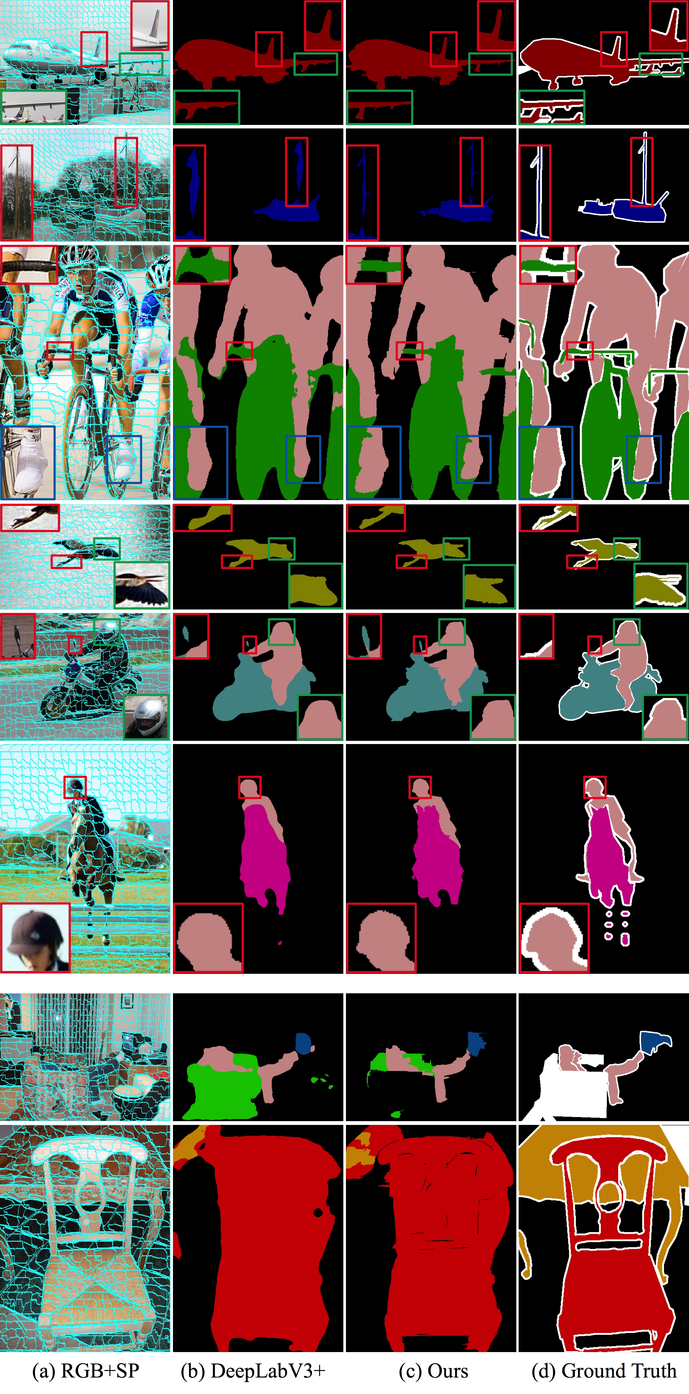
Applying superpixel contours increased the mIoU from 77.78% to 78.15%, based on which fine-tuning by our transparent initialization further increased it by 0.79% (1.16% to DeepLabV3+). Pretrained on MS-COCO for PASCAL VOC 2012, our proposal has 0.61% increase of mIoU. Note that most edges in the ground truth were neglected in the evaluation, marked white in Fig. 5(d).
Again, our goal is to preserve sharp edges aligned with object contours by superpixels. Fig. 5 vividly shows the enhanced object edges, especially objects that are highly contrastive to the background, such as birds and human heads.
| Manner | Backbone | SP | TI | MS-COCO | mIoU (/full) |
| DeepLabV3+ [9] | ResNet101 | - | - | - | 78.85 / 76.47 |
| Ours | ResNet101 | ✓ | - | - | 79.22 / 76.98 |
| DeepLabV3+ [9] | ResNet152 | - | - | - | 79.32 / 77.78 |
| Ours | ResNet152 | ✓ | - | - | 79.94 / 78.15 |
| ResNet152 | ✓ | ✓ | - | 80.46 / 78.94 | |
| DeepLabV3+ [9] | ResNet152 | - | - | ✓ | 82.62 / 80.76 |
| Ours | ResNet152 | ✓ | ✓ | ✓ | 83.39 / 81.37 |
| Manner | pixAcc. | mIoU |
| PSPNet [55] | 81.39 | 43.29 |
| EncNet [53] | 81.69 | 44.65 |
| ResNeSt50 [54] | 81.17 | 45.12 |
| ResNeSt101 [54] | 82.07 | 46.91 |
| Ours333Since [54] has 64 GPUs for state-of-the-art ResNeSt training while only 4 GPUs are accessible for ours, we used ResNeSt101 as baseline. | 82.37 | 47.42 |
| Manner | pixAcc. | mIoU |
| FCN (ResNet50) [34] | 73.40 | 41.00 |
| EncNet [53] | 80.70 | 54.10 |
| ResNeSt50 [54] | 80.41 | 53.19 |
| ResNeSt101 [54] | 81.91 | 56.49 |
| Ours333Since [54] has 64 GPUs for state-of-the-art ResNeSt training while only 4 GPUs are accessible for ours, we used ResNeSt101 as baseline. | 82.43 | 57.32 |
4.4 Evaluations
Semantic Segmentation.
For ADE20K and PASCAL Context, we used the most recent state-of-the-art semantic segmentation network ResNeSt [54] 222https://github.com/zhanghang1989/PyTorch-Encoding. Its state-of-the-art performance on ADE20K using ResNeSt200 is 82.45% pixel accuracy and 48.36% mIoU, and 83.06% pixel accuracy and 58.92% mIoU on PASCAL Context using ResNeSt269. Since we have only 4 P100 (16 GB) GPUs for our experiments while [54] has 64 V100 (16 GB) GPUs, we chose ResNeSt101 instead of ResNeSt200 or ResNeSt269 as our baseline network. Note that it is possible to enhance semantic segmentation edges on those state-of-the-art networks given sufficient GPU memory.
In Table 5, our method improves the pixel accuracy by 0.39% and mIoU by 0.61% on ADE20K over the baseline. In Table 6, the pixel accuracy is improved by 0.71% and the mIoU by 0.83% over the baseline.
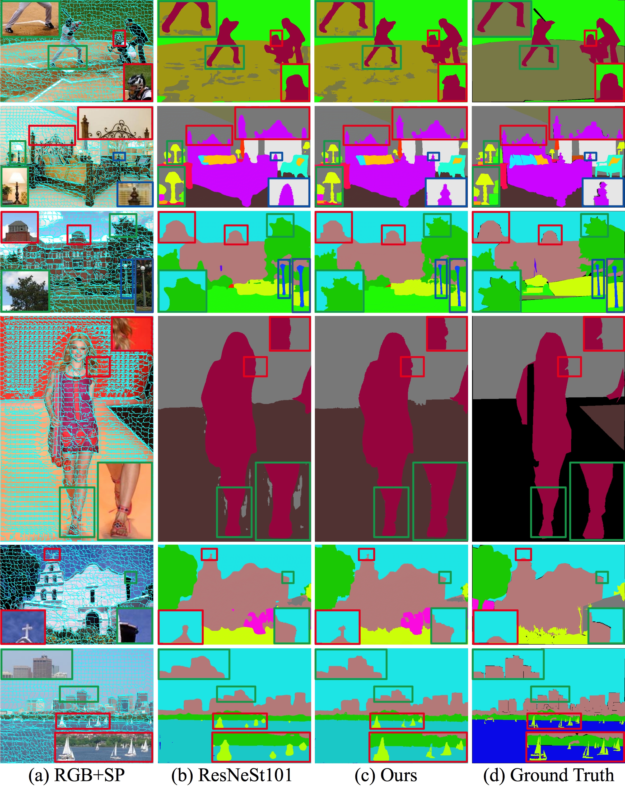
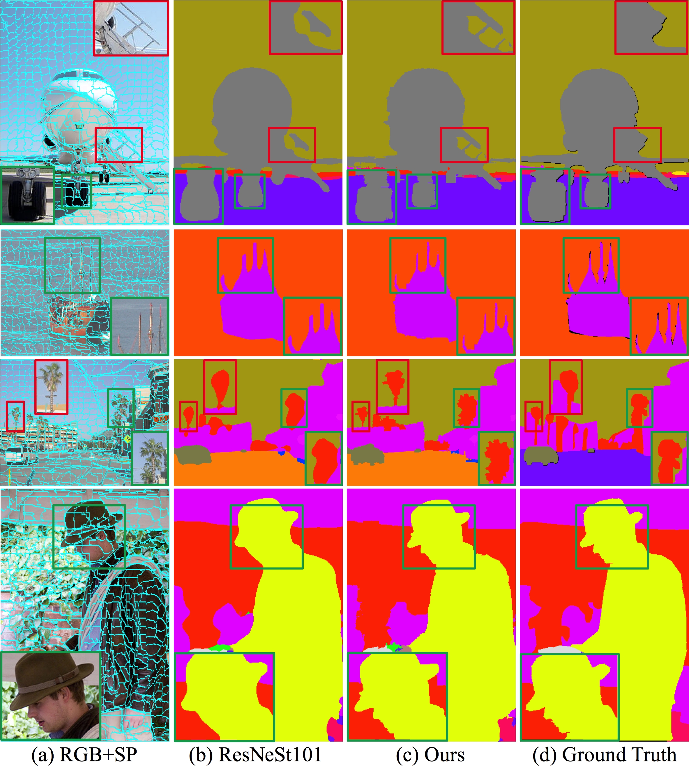
More importantly, visualizations in Fig. 6 for ADE20K and Fig. 7 for PASCAL Context vividly show the enhanced object edge details. This is the core of our refinement on semantic segmentation with superpixel constraints. For a fair comparison with [54], multiscale evaluations with multiscale superpixel maps were used while the superpixel maps in Figs. 6-7 are single-scale merely for demonstration.
Semantic Segmentation Edges.
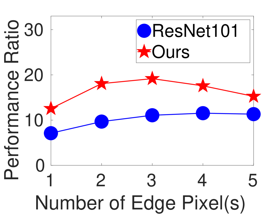
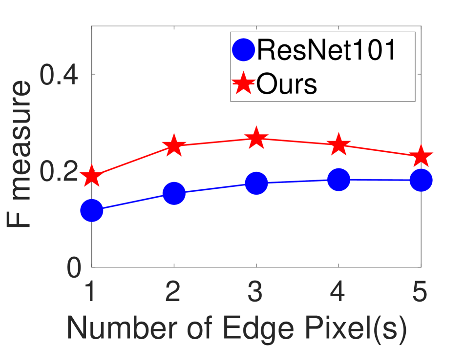
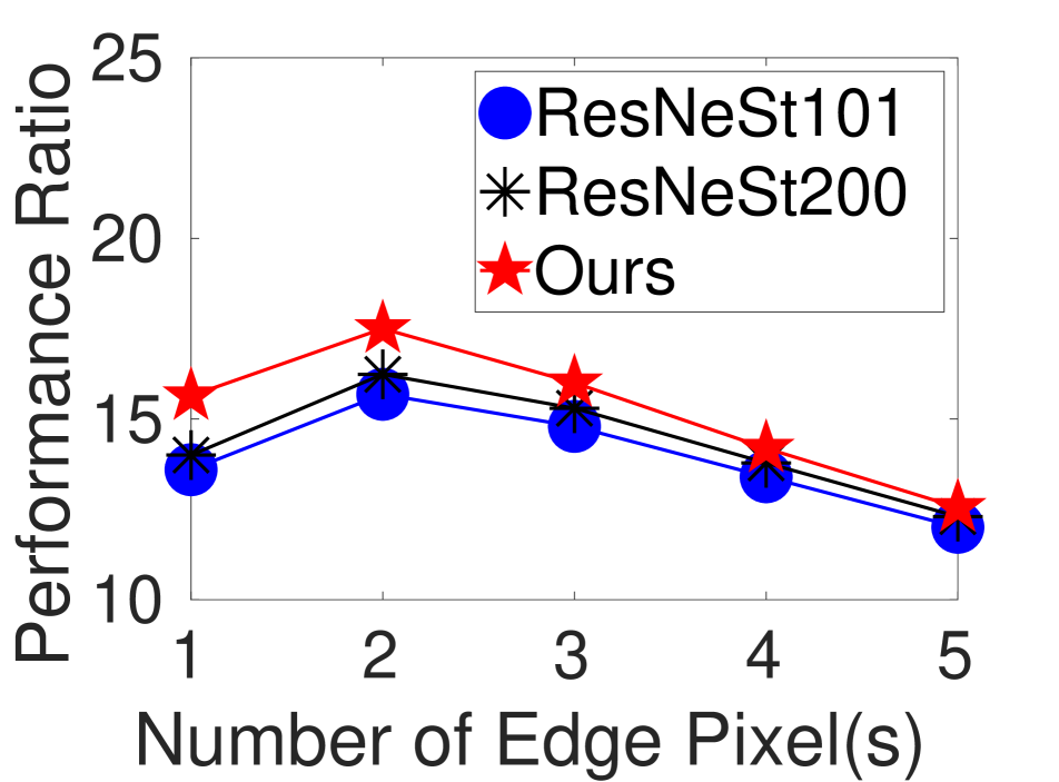
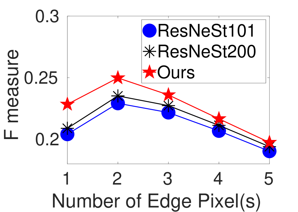
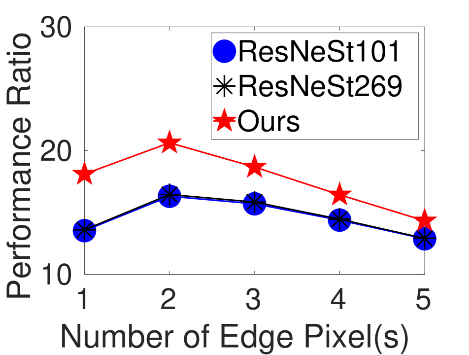
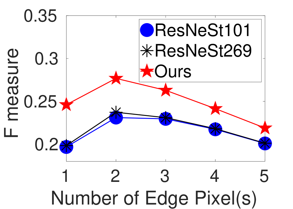
Since our refinement of semantic segmentation mainly lies in object edge areas, we used the popular Performance Ratio (PR) [27] and F-measure (FM) [42, 15] to evaluate the enhanced segmentation edges. In Fig. 8, ours outperform the baselines, i.e., ResNet101 on PASCAL VOC 2012 and ResNeSt101 on the others, as well as the most recent state-of-the-art [54], i.e., ResNeSt200 on ADE20K and ResNeSt269 on PASCAL Context, with higher PR and FM. Illustrations of the state-of-the-art edges compared with ours are shown in Fig. 1.
5 Conclusion
With transparent initialization and sparse encoder introduced in our paper, the joint learning of the state-of-the-art networks for semantic segmentation and superpixels preserves object edges. The proposed transparent initialization used to fine-tune pretrained models retains the effect of learned parameters through identically mapping the network output to its input at the early learning stage. It is more robust and effective than other parameter initialization methods, such as Xavier and Net2Net. Moreover, the sparse encoder enables the feasibility of efficient matrix multiplications with largely reduced computational complexity. Evaluations on PASCAL VOC 2012, ADE20K, and PASCAL Context datasets validate the effectiveness of our proposal with enhanced object edges. Meanwhile, the quality of our semantic segmentation edges, evaluated by performance ratio and F-measure, is higher than other methods Additionally, transparent initialization is not limited to the joint learning for semantic segmentation but can also be used to initialize additional fully-connected layers for other tasks such as deep knowledge transfer.
Acknowledgement
We would like to thank the Australian National University, the Australian Centre for Robotic Vision (CE140100016), and Data61, CSIRO, Australia, for supporting this work.
Appendix
This provides additional details about transparent layers, giving more details of the initialization and structure of the layers. In particular, it shows how the approach may be used for any activation functions, not only forms of ReLU that were discussed in the main paper. This also speculates about the application of these ideas to form transparent convolutional layers. We now describe the ideas at a slower pace than is possible in the main paper, sometimes using different notation.
Appendix A Introduction for Warmup
A common technique is to extend an existing network by the addition of further affine layers (classification layers) before the loss layer. These layers may then be trained separately or the whole extended network can be trained. We refer to the original (unextended) network as the base-network, and the network extended by some additional layers as the extended network. We assume that the extension layers consist of fully-connected layers, including offset, followed by an activation layer, such as a ReLU. These extension layers are inserted before the loss-layer.
Assuming that the base layer is trained to attain a low value of the loss, we wish to insert the extension layers into the network without increasing the loss of the network, so that additional training may continue to decrease the value of the loss-function. However, if the extension layers are initialized with random parameters, it will result in an increase in the loss of the network, so that the extension layers, or the whole network needs to be trained from scratch.
Simple transparent layers.
This problem has also been addressed in previous work of Goodfellow [10]. One very simple method to implement a transparent layer is to let the matrix of layer parameters be the identity matrix. This has the disadvantage, however, that all the parameters are either or , which fails to introduce sufficient randomness into the system, which would perhaps be desirable. In addition, if the function is represented by the identity mapping, then many of the parameters are equivalent, perhaps also an undesirable feature. We wish to allow the parameters of the affine transformation to be chosen randomly so as to mix things up a bit.
It is also not clear to do in the case where , where , for then there is no such thing as an identity matrix. We wish to allow the possibility that the output and input of the extension layers are not equal.
Appendix B Affine Layers
We are interested in layers in a Neural Network (NN) that implement an affine transformation on the input, that is, a linear transformation followed by an offset. For the present, we ignore any non-linear activatation that might be applied to the output of the layer.
The most obvious example of such a layer is a fully-connected layer, and that will be our main focus. However, the same idea could be applied to handle convolution layers. We raise this possibility and make a few comments on this later. Any development of this idea is left to further work.
An affine layer, in the following discussion, is seen as composed of a linear transform, followed by an offset and then a non-linear activation. The linear transform, followed by offset performs an affine transformation on the data, which will be written as333 The notation in this exposition differs slightly, mainly in choice of fonts, from the main paper. Here, we deonte a matrix by , an affine transformation by and the matrix that expresses an affine transformation in terms of homogeneous coordinates by . Homogeneous quantities in general (such as homogeneous vectors are denoted with a tilde).
| (15) |
where . In this note, the convention is that vectors, such as are row vectors, which is contrary to a convention common in computer vision literature that vectors represent column vectors. The present notation is common in computer graphics literature, however.
This mapping satisfies the condition
| (16) |
and it may be represented by matrix multiplication on the homogenized vector , according to
| (17) |
where the matrix is given by
| (18) |
For future reference, the matrix that performs the inverse affine transformation is equal to
| (19) |
This works if is a square matrix and has an inverse. More generally, in the case where is of dimension , with , it is possible that has a right-inverse, which is a matrix, denoted by such that . In this case, a right inverse for is given by
| (20) |
where is the right-inverse of matrix .
An affine transform maps onto an affine subspace of , and the rank of the affine transform may be defined as the dimension of the affine space that is the image of this transform. Such a transformation will be said to be of full rank if its rank is equal to , the dimension of input space.
From here on, we shall use the symbol to represent an affine transformation, writing . The symbol represents the transformation itself, not the matrix (in this case ) that implements it. Caution: to reemphasize this, the symbols and do not represent the same thing. In particular is a matrix and is an affine transform, which is equivalent to matrix multiplication by a matrix and offset by a vector , so that is short-hand notation for .
Interlude: right inverse of a matrix.
Let be an matrix with . An matrix is the right-inverse of if . Such a matrix exists if and only if has rank equal to its row-dimension. This cannot happen if , where a right-inverse cannot exist.
In this case, is given by the formula
| (21) |
where the condition is easily verified. This formula relies on the fact that ⊤ has an inverse, which is ensured because the rank of is .
An alternative procedure is to take the Singular Value Decomposition (SVD) , where ⊤ has dimension and . The matrix (of dimension ) is non-singular (since has rank ). Then, the right-inverse is given by
| (22) |
as is easily verified.
Appendix C Sequences of Layers without Activation
For the time being, we consider the unrealistic case that the activation layer is missing from the affine layers. In this case, each affine layer performs an affine transformation. A sequence of transformations may be applied to an input , giving
| (23) |
If we choose to be a right-inverse of then we have
| (24) |
the identity mapping.
The condition for this right inverse to exist is that should be of full rank. A necessary condition for this to happen is as follow. Let represent an affine transformation . The first and last spaces in this sequence are and , so and . Then has a right inverse only if for all . In other words, a necessary condition for the right inverse to exist is that the dimensions of all the intermediate spaces should be at least equal to . It is not hard to see that generically, this is also a sufficient condition, meaning that it is true for almost all sequences of transformations.444The terms almost all, almost always, etc. are intended in the standard mathematical sense, meaning that the set of cases for which the relevant condition fails to be true has measure or probability zero. For instance the set of , with that do not have full rank is a set of measure in the set of all such matrices, so one can state that almost all such matrices have full rank. As another example, a matrix chosen at random (which implies that numbers are chosen from some probability distribution such as a normal distribution) will be of full rank with probability , hence almost always.
Without being too formal here, we can state that this condition will hold generically if all the transformations are chosen at random.
Theorem 2
Let a sequence of affine transformations , for be chosen at random. Then almost surely has a right inverse if and only if for .
For practical purposes it is safe to proceed as if this result holds always (and not just almost always), since the probability that does not have an inverse is vanishingly small (in fact zero).
Therefore, the strategy for selecting a set of parameters for a sequence of affine layers may be described. For the sequence of layers to represent an identity transform, we need that the input and output space have the same dimension, namely . Then
-
1.
Select intermediate dimensions such that for all .
-
2.
Define random affine transforms by selecting the entries of matrices and vectors randomly, using a suitable random number generator, for instance by a zero-mean normal (Gaussian) distribution.
-
3.
Compute the composition by matrix multiplication, and take its right-inverse.
-
4.
Set to equal .
The resulting product is the identity affine transformation.
Appendix D Gaussian Random Matrices
Since we are using matrices initialized from a normal distribution, we give some properties of such matrices. The purpose is to ensure that the concatenation of affine transformations does not cause explosion of the entries of the product . If this is not done properly, then this product will have very large entries and so will any value of .
The solution is to make the matrices appearing as the linear-transform part of as close to orthogonal as possible. As an additional advantage, the entries of will be approximately of the same order as the entries of each of the other . It will turn out that the entries of each should be chosen from a Gaussian distribution with variance where is its row-dimension.
We are assuming here that the dimensions of the matrix are large. In addition, if the matrix is not square, by saying it is orthogonal we mean that both its rows (and similarly it columns) are orthogonal vectors, all of the same length (a different length for the row and column vectors, of course). One may mistakenly assume that by randomly selecting each entry of a matrix randomly one obtains a random matrix in some vague sense. In reality, one obtains an (nearly) orthogonal matrix.
To see this, we first see that two random vectors from distribution are almost orthogonal. Let and be two i.i.d random variables in , we have
| (25) |
and
| (26) |
Then,
| (27) | ||||
Now, given a column vector with entries chosen from distribution , we have
| (28) |
where and are independent entries in two of such column vectors respectively. Then, the expected squared length of such a vector is . If we choose , has the expected squared length equal to 1. This satisfies the attribute of an orthogonal matrix, . Then, Eq. (27) follows
| (29) |
Hence, two -length vectors randomly chosen from will have expected squared length 1 and expected inner-product 0 (by Eq. (25)) with variance of the inner product as .
On the other hand, the variance of the square length of the vector is
| (30) |
where is obtained by with and
| (31) | ||||
To this end, it shows
Theorem 3
If entries of an matrix are chosen from a zero-mean distribution with variance , then the column vectors have expected squared length 1 with variance and the expected inner product of each two columns is 0 with variance .
As increases, the matrix approximates more and more an orthogonal matrix. Corresponding to Fig. 4 in the main paper, weights and bias can be initialized by
-
1.
Choose the dimension of -th layer filter as , for , where .
-
2.
Define a random affine transformation by selecting its weight matrix from a Gaussian distribution and its bias vector from a Gaussian distribution.
-
3.
Initialize with the right inverse of .
Again, note that is an affine transformation (also used as a layer) where is the weight matrix of . Then, the above initialization will lead to an identity mapping as .
Appendix E Getting Past the Activation Layer
We concentrate first on the case where each affine transform is followed by a ReLU activation. To do this, we will need to double the size of the intermediate layers, as will be seen next. We assume that affine transforms are given, let be the input of and define for , the output of the -th affine transform.
In the course of the following discussion, we shall be defining new affine transforms and layers represented by , namely an affine transform followed by an activation . Once more let be the input of the first layer, , and define , the result of the affine transformation followed by the activation. Quantities without primes ( and ) belong to the original sequence of affine transforms, whereas those with primes ( and ) belong to the sequence, with activation, being constructed).
The first layer will be modified as follows. Suppose that is represented in matrix form as
| (32) |
This is replaced by
| (33) | ||||
In other words, the matrix is replaced by the matrix , and is replaced by the dimensional vector .555 Important note: The affine transformation is defined This will output a vector of the form with two parts that are negatives of each other. It defines the initial form of the affine transform only. During training, all entries of the above matrix are free to vary (and will) independently, and its output will not maintain this symmetric form. This applies to all the affine transforms that will be defined.
Now, when this is passed through an activation layer, represented by the activation function (ReLU), the result is
| (34) |
This is the output of our modified affine layer with activation. The point to note here is the identity . This gives
| (35) |
Thus, by subtracting the two halves of , one arrives back at the simple affine transform .
We simplify the notation as follows. Let and be defined as
| (36a) | ||||
| (36b) | ||||
which are the positive and negative parts of respectively, satisfying . Then, we see that
| (37) |
Now, the first thing to do at the beginning of the next layer is to subtract the two parts of the previous output, illustrated by
| (38) |
This is followed by the same trick of separating the positive and negative parts as before. The affine part (without activation) of the second layer is then
| (39) | ||||
where , and are defined by this equation. Noting Eq. (38), we arrive at
| (40) |
and so
| (41) |
Combining this with Eq. (37) gives
| (42) |
Continuing to define layers in this way, according to Eq. (44), for layers up to layer , gives that
| (43) |
Finally, we define the last layer by
| (44) | ||||
Putting those defined all together gives
| (45) |
where the final step is because the sequence of affine transforms is chosen to be the identity map, so .
Appendix F Exploration of Layer Initialization Effects
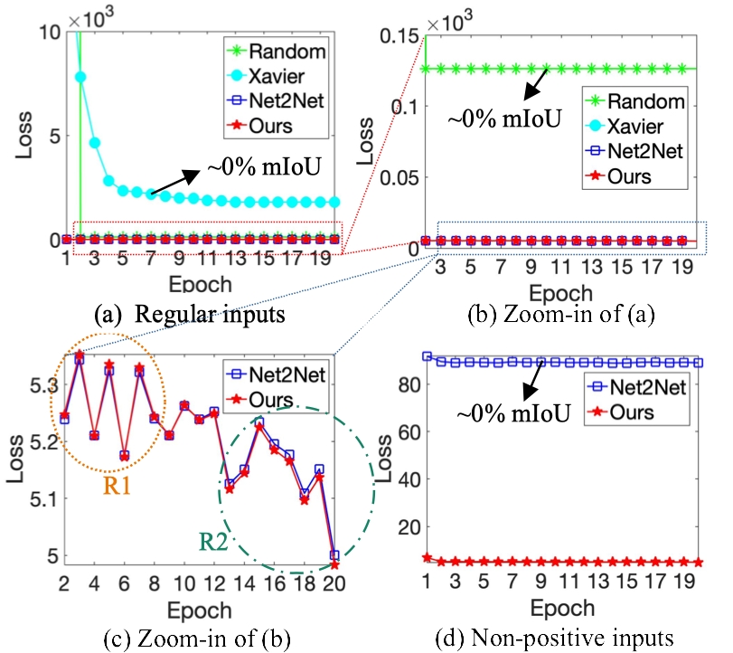
In Table 2 in the main paper, we compared the effectiveness of our transparent initialization with others, that is random, Xavier [18], and Net2Net [10]. Transparent initialization can 100% recover the input data from the layers output with a high initialization rate and a small around-off error shown in Table 3 and supports non-square filters, by saying filters we mean kernel-size convolutional layers or fully-connected layers. In contrast, random and Xavier initialization are ineffective to recover the input data from the output while Net2Net is only effective for non-negative data and is infeasible for non-square filters. Despite these quantitative experiments to analyse the attributes of transparent initialization, we directly compare their effects on joint learning pretrained networks of semantic segmentation and superpixels in addition to the ablation study in the main paper.
In Fig. 9, for the task of semantic segmentation, the cross-entropy loss function highly relies on the maximum values of logits, the network outputs, along the label dimension. In Fig. 9(a)-9(c), input data of the add-on FC layers contains positive and non-positive values while in Fig. 9(d) input data is non-positive by subtracting the maximum value along the label dimension. This is to explore the data recovering ability for different numerical space (that is non-negative and non-positive in our case).
The final mIoUs via random and Xavier initialization are nearly 0% as they totally interrupt the learned parameters, leading to a high loss. To recover non-negative data, in Fig. 9(c), Net2Net and ours have similar loss decreasing tendency. However, as the epoch increases, the loss by ours becomes lower than Net2Net because the gradients by transparent initialization are dense for parameter updates compared with the sparse ones by Net2Net. Furthermore, in Fig. 9(d), Net2Net is unable to recover negative values, as shown in Table 2 in the main paper, resulting in a high loss. In Fig. 9(c), the mIoU by Net2Net and ours are similar, both nearly 83.3%. Corresponding to Fig. 9(d), however, the mIoU by Net2Net is nearly 0% while ours is still nearly 83.3% since it is invariant to numerical space.
Appendix G Activation Functions
Again, note that the notation of activation function has the same meaning as for a simplicity of sequence layers. For the proposed transparent initialization, any non-linear activation functions satisfying Eq. (46) are feasible to recover the input data from its output.
| (46) |
where is a non-zero constant. This can be expressed by with (duplicate) and (subtract) defined in the main paper. In Fig. 10, we give 4 examples with corresponding definitions as follows:
| ReLU: | (47c) | |||
| LeakyReLU: | (47f) | |||
| SoftReLU: | (47g) | |||
| LogSigmoid: | (47h) | |||
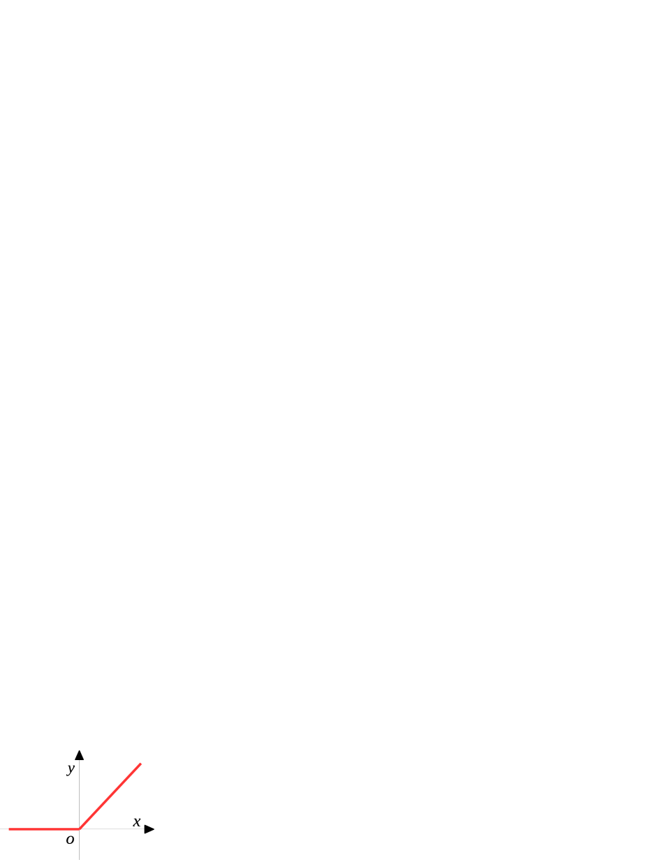


It is easy to verify Eq. (46) for those activation functions. Given the activation function as LogSigmoid by , for instance, it follows
| (48) | ||||
Meanwhile, with given in Eq. (46), should be , where is for LeakyReLU and for the others. To be more general, this property holds for any functions of the form of , where is an even function.
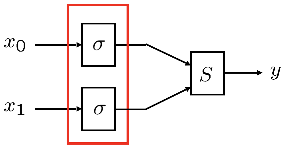
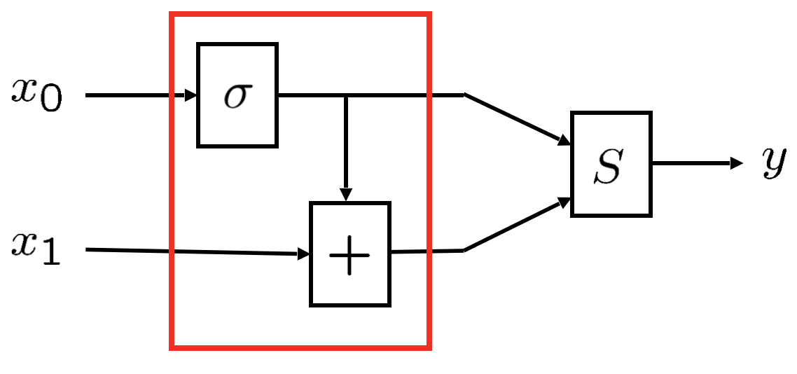
For other activations such as the sigmoid function, or arctangent, or hyperbolic tangent, it does not work directly. The trick is to observe that for the ReLU function, . This allows us to rewrite the sequence of operations
where is the ReLU function, as
But now this also holds for any activation , ReLU or not. This requires a slight change to the architecture of the transparent affine layer. Instead of outputting , it must output . This is shown in Fig. 11.
Appendix H Extension to Convolutional Layers
A common practice in experimenting with modifications to neural network architectures is to add additional convolutional layers. If a base network is already trained to achieve minimal loss, then the addition of extra convolutional layers can perturb the loss, and require the network to retrain again to achieve a low loss. The loss after addition of the new layers may not be as low as the loss of the base network. However, by initializing the extra add-on layers to implement an identity transformation will ensure that the loss achieved (on the training set) by the modified network cannot be worse than that of the base network.
This section gives some ideas on the addition of transparent convolutional layers with pseudo-random initialization that could be used for this purpose. We have not explored this topic in any great depth, leaving it rather to be the subject of future work, and is somewhat speculative at present.
A convolutional layer as usually implemented is an example of an affine layer, since without any non-linear activation it implements a linear transformation on the input and then adds bias. However, unlike fully-connected layers, which are essentially a matrix multiplication, for which an inverse (or right-inverse) can be easily found, convolution is not conveniently represented by matrix multiplication and is less easily inverted.
It is clear that convolution, being linear, can be represented as matrix multiplication on a vectorized form of the input, but this will be a sparse matrix multiplication, and not easily inverted, at least by convolutional layers. By analogy with the method implemented for fully-connected layers, we require that a final convolution will invert the effect of a sequence of previous pseudo-random convolutions.
Not all convolutions are exactly invertible. In fact (ignoring edge effects) a convolution will be invertible by another convolution if and only if its Fourier transform is everywhere non-zero. However, with this caveat, it is possible to find inverse convolutions.
Rather than carrying out a string of convolutions, followed by a single convolution to undo the previous ones, a better strategy may be to add convolutions in pairs such as a high-pass and low-pass filter that cancel each other out. Exploring this topic will be the subject of further work.
References
- [1] R. Achanta, A. Shaji, K. Smith, A. Lucchi, P. Fua, and S. Susstrunk. SLIC superpixels compared to state-of-the-art superpixel methods. TPAMI, 34(11):2274–2282, 2012.
- [2] R. Achanta and S. Susstrunk. Superpixels and polygons using simple non-iterative clustering. CVPR, 2017.
- [3] T. Ajanthan, A. Desmaison, R. Rudy, M. Salzmann, P.H.S. Torr, and M.P. Kumar. Efficient linear programming for dense CRFs. CVPR, 2017.
- [4] P. Arbelaez, M. Maire, C. Fowlkes, and J. Malik. Contour detection and hierarchical image segmentation. TPAMI, 33(5):898–916, 2010.
- [5] V. Badrinarayanan, A. Kendall, and R. Cipolla. SegNet: A deep convolutional encoder-decoder architecture for image segmentation. TPAMI, 39(12):2481–2495, 2017.
- [6] M.V. Bergh, X. Boix, G. Roig, and L.V. Gool. SEEDS: Superpixels extracted via energydriven sampling. IJCV, 2015.
- [7] L.C. Chen, J.T. Barron, G. Papandreou, K Murphy, and A.L. Yuille. Semantic image segmentation with task-specific edge detection using CNNs and a discriminatively trained domain transform. CVPR, 2016.
- [8] L.C. Chen, G. Papandreou, I. Kokkinos, K. Murphy, and A.L. Yuille. DeepLab: Semantic image segmentation with deep convolutional nets, atrous convolution,and fully connected CRFs. TPAMI, 40(4):834–848, 2017.
- [9] L. Chen, Y. Zhu, G. Papandreou, F. Schroff, and H. Adam. Encoder-decoder with atrous separable convolution for semantic image segmentation. ECCV, 2018.
- [10] T. Chen, I. Goodfellow, and J. Shlens. Net2Net: Accelerating learning via knowledge transfer. ICLR, 2016.
- [11] Y. Chen, Y. Kalantidis, J. Li, S. Yan, and J. Feng. A2-nets: Double attention networks. NeurIPS, 2018.
- [12] J. Deng, W. Dong, R. Socher, L.J. Li, K. Li, and F. Li. ImageNet: A large-scale hierarchical image database. CVPR, 2009.
- [13] M. Everingham, S.M.A. Eslami, L.V. Gool, C.K.I. Williams, J. Winn, and A. Zisserman. The pascal visual object classes challenge a retrospective. IJCV, 2014.
- [14] D. Feng, C.H. Schutz, L. Rosenbaum, H. Hertlein, C. Glaser, F. Tim, W. Wiesbeck, and K. Dietmayer. Deep multi-model object detection and semantic segmentation for autonomous driving: Datasets, methods, and challenges. IEEE Transactions on Intelligent Transportation systems, pages 1–20, 2020.
- [15] P.A. Flach and M. Kull. Precision-recall-gain curves: Pr analysis done right. NeurIPS, 2015.
- [16] J. Fu, J. Liu, H. Tian, Y. Li, Y. Bao, Z. Fang, and H. Lu. Dual attention network for scene segmentation. CVPR, 2019.
- [17] R. Gadde, V. Jampani, M. Kiefel, D. Kappler, and P.V. Gehler. Superpixel convolutional networks using bilateral inceptions. ECCV, 2016.
- [18] X. Glorot and Y. Bengio. Understanding the difficulty of training deep feedforward neural networks. AISTATS, 2010.
- [19] S. Gould, J. Zhao, X. He, and Y. Zhang. Superpixel graph label transfer with learned distance metric. ECCV, 2014.
- [20] K. He, X. Zhang, S. Ren, and J. Sun. Deep residual learning for image recognition. CVPR, 2016.
- [21] M. Hofmarcher, T. Unterthiner, J.A. Medina, G. Klambauer, S. Hochreiter, and B. Nessler. Visual scene understanding for autonomous driving using semantic segmentation. Explainable AI. LNCS, 11700:285–296, 2019.
- [22] S. Hong, X. Yan, T. Huang, and H. Lee. Learning hierarchical semantic image manipulation through structured representations. NeurIPS, 2018.
- [23] G. Huang, Z. Liu, L.V.D. Maaten, and K.Q. Weinberger. Densely connected convolutional networks. CVPR, 2017.
- [24] P. Isola, D. Zoran, D. Krishnan, and E.H. Adelson. Crisp boundary detection using pointwise mutual information. ECCV, 2014.
- [25] V. Jampani, D. Sun, M.Y. Liu, M.H. Yang, and J. Kautz. Superpixel sampling networks. ECCV, 2018.
- [26] M. Jordan. Learning in graphical models. MIT Press, 1998.
- [27] P.A. Khaire and Dr.N.V. Thakur. A fuzzy set approach for edge detection. International Journal of Image Processing, 6(6):403–412, 2012.
- [28] P. Krahenbuhl and V. Koltun. Efficient inference in fully connected CRFs with Gaussian edge potentials. NeurIPS, 2011.
- [29] X. Li, Z. Zhong, J. Wu, Y. Yang, Z. Lin, and H. Liu. Expectation-maximization attention networks for semantic segmentation. ICCV, 2019.
- [30] Z. Li and J. Chen. Superpixel segmentation using linear spectral clustering. CVPR, 2015.
- [31] G. Lin, A. Milan, C. Shen, and I. Reid. RefineNet: Multi-path refinement networks for high resolution semantic segmentation. CVPR, 2017.
- [32] T.Y. Lin, M. Maire, S. Belongie, L. Bourdev, R. Girshick, J. Hays, P. Perona, D. Ramanan, C.L. Zitnick, and P. Dollar. Microsoft COCO: Common objects in context. ECCV, 2014.
- [33] Y.J. Liu, C.C. Yu, M. Yu, and Y. He. Manifold SLIC: A fast method to compute content-sensitive superpixels. CVPR, 2015.
- [34] J. Long, E. Shelhamer, and T. Darrell. Fully convolutional networks for semantic segmentation. CVPR, 2015.
- [35] D. Martin, C. Fowlkes, D. Tal, and J. Malik. A database of human segmented natural images and its application to evaluating segmentation algorithms and measuring ecological statistics. ICCV, 2001.
- [36] R. Mottaghi, X. Chen, X. Liu, N.G. Cho, S.W. Lee, S. Fidler, R. Urtasun, and A. Yuille. The role of context for object detection and semantic segmentation in the wild. CVPR, 2014.
- [37] H. Park, J. Jeong, Y. Yoo, and N. Kwak. Superpixel-based semantic segmentation rrained by statistical process control. BMVC, 2017.
- [38] N.O. Salscheider. Simultaneous object detectin and semantic segmentation. International conference on pattern recognition applications and methods (ICPRAM), 2019.
- [39] F. Schroff, A. Criminisi, and A. Zisserman. Object class segmentation using random forests. BMVC, 2008.
- [40] M. Schuurmans, M. Berman, and M.B. Blaschko. Efficient semantic image segmentation with superpixel pooling. arXiv preprint arXiv:1806.02705, 2018.
- [41] K. Simonyan and A. Zisserman. Very deep convolutional networks for large-scale image recognition. ICLR, 2015.
- [42] D. Stutz, A. Hermans, and B. Leibe. Superpixels: An evaluation of the state-of-the-art. Computer Vision and Image Understanding, 166:1–27, 2018.
- [43] D. Stutz, A. Hermans, and B. Leibe. Superpixels: An evaluation of the state-of-the-art. CVIU, 2018.
- [44] I. Sutskever, J. Martens, G. Dahl, and G. Hinton. On the importance of initialization and momentum in deep learning. ICML, 2013.
- [45] M. Thoma. A survey of semantic segmentation. arXiv:1602.06541, 2016.
- [46] W.C. Tu, M.Y. Liu, V. Jampani, D. Sun, S.Y. Chien, M.H. Yang, and J. Kautz. Learning superpixels with segmentation-aware affinity loss. CVPR, 2018.
- [47] R. Uziel, M. Ronen, and O. Freifeld. Bayesian adaptive superpixel segmentation. ICCV, 2019.
- [48] P. Wang, G. Zeng, R. Gan, J. Wang, and H. Zha. Structure-sensitive superpixels via geodesic distance. IJCV, 2013.
- [49] X. Wang, T. Wang, and J. Bu. Color image segmentation using pixel wise support vector machine classification. pattern recognition, 2011.
- [50] F.Z. Xing, E. Cambria, W.B. Huang, and Y. Xu. Weakly supervised semantic segmentation with superpixel embedding. ICIP, 2016.
- [51] B. Xu, N. Wang, T. Chen, and M. Li. Empirical evaluation of rectified activations in convolutional network. arXiv:1505.00853, 2015.
- [52] F. Yang, Q. Sun, H. Jin, and Z. Zhou. Superpixel segmentation with fully convolutional networks. CVPR, 2020.
- [53] H. Zhang, K. Dana, J. Ping, Z. Zhang X. Wang, A. Tyagi, and A. Agrawal. Context encoding for semantic segmentation. CVPR, 2018.
- [54] H. Zhang, C. Wu, Z. Zhang, Y. Zhu, Z. Zhang, H. Lin, Y. Sun, T. He, J. Mueller, R. Manmatha, M. Li, and A. Smola. ResNeSt: Split-attention networks. arXiv:2004.08955, 2020.
- [55] H. Zhao, J. Shi, X. Qi, X. Wang, and J. Jia. Pyramid scene parsing network. CVPR, 2017.
- [56] H. Zhao, Y. Zhang, S. Liu, J. Shi, C.C. Loy, D. Lin, and J. Jia. PSANet: Point-wise spatial attention network for scene parsing. ECCV, 2018.
- [57] S. Zhao, Y. Wang, Z. Yang, and D. Cai. Region mutual information loss for semantic segmentation. NeurIPS, 2019.
- [58] Shuai Zheng, S. Jayasumana, B.R. Paredes, V. Vineet, Z. Su, D. Du, C. Huang, and P.H.S. Torr. Conditional random fields as recurrent neural networks. ICCV, 2015.
- [59] B. Zhou, H. Zhao, X. Puig, S. Fidler, A. Barriuso, and A. Torralba. Scene parsing through ade20k dataset. CVPR, 2017.
- [60] B. Zhou, H. Zhao, X. Puig, T. Xiao, S. Fidler, A. Barriuso, and A. Torralba. Semantic understanding of scenes through ade20k dataset. IJCV, 2016.