Performance Analysis of a Two–Tile Reconfigurable Intelligent Surface Assisted $2\times 2$ MIMO System

Abstract

We consider a two–tile reconfigurable intelligent surface (RIS) assisted wireless network with a two-antenna transmitter and receiver over Rayleigh fading. We show that the average received signal-to-noise-ratio (SNR) optimal transmission and combining vectors are given by the left and right singular spaces of the RIS-receiver and transmit-RIS channel matrices, respectively. Moreover, the optimal phases at the two tiles of the RIS are determined by the phases of the elements of the latter spaces. To further study the effect of phase compensation, we statistically characterize the average SNR of all possible combinations of transmission and combining directions pertaining to the latter singular spaces by deriving novel expressions for the outage probability and throughput of each of those modes. Furthermore, for comparison, we derive the corresponding expressions in the absence of RIS. Our results show an approximate SNR improvement of $2$ dB due to the phase compensation at the RIS.

I Introduction

Reconfigurable intelligent surfaces (RISs) have been identified as one of the possible physical-layer technologies for beyond-5G networks. RIS can passively beamform the received signal from a wireless transmitter towards its receiver by using large arrays of antenna elements which are usually spaced half of the wavelength apart [1]. Since the benefit of RISs can only be achieved by properly configured phase shifts of passive reflective elements in real time, most existing work on RISs focus on phase optimization, see e.g., [2, 3, 4] and references therein. In contrast, communication-theoretic performance limits of RIS assisted single-antenna systems have been analyzed in [5, 6, 7, 8, 9, 10]. However, few research efforts explored the performance of multi-antenna systems [11].

For a large number of elements at the RIS, the authors of [12] investigate an RIS-assisted multiple-input and multiple-output (MIMO) network. Exact analytical characterization of finite dimensional RIS-assisted systems, on the other hand, is not available in the current literature. Therefore, different from previous works, this paper analytically characterizes the exact performance, in terms of outage probability and throughput, of a fundamental finite dimensional RIS-assisted MIMO system. In particular, we focus our attention on a $2\times 2$ MIMO system model assisted by an RIS made of two tiles that can be configured to operate as anomalous or conventional reflectors by adjusting independently their surface phase shifts [13].

We propose an analytical framework based on the representation of the $2\times 2$ unitary group of matrices to represent the average signal-to-noise-ratio (SNR) optimal transmission and receive strategies along with the optimal phase adjustments at the RIS over Rayleigh fading. We prove that the left and right singular spaces of the RIS-receiver and transmit-RIS channel matrices are optimal in the above sense. Capitalizing on this, we exploit results from finite dimensional random matrix theory (see e.g., [14]) to characterize the outage and throughput with and without the phase adjustment of the tiles of the RIS for each of the latter strategies. Moreover, numerical results show that the proposed (suboptimal) strategy achieves comparable performance as the alternating optimal strategy based on jointly optimized instantaneous SNR. In particular, the throughput of the proposed scheme provides a tight lower bound for the throughput corresponding to the latter strategy.

Notations: $\mathbb{E}\{\cdot\}$, $(\cdot)^{\dagger}$, $(\cdot)^{T}$, $||\cdot||$, $\text{Tr}(\cdot)$, $\text{diag}(\ldots)$, $|\cdot|$, $(\cdot)^{*}$, $\text{arg}(\cdot)$, and $\mathcal{U}_{2}$ denote the mathematical expectation, the Hermitian transpose operator, the conjugate operator, the transpose operator, the $\ell_{2}$ norm of a vector, the trace of a matrix, a diagonal matrix, the modulus of a complex number, the complex conjugation operation, the argument of a complex number, and the group of $2\times 2$ unitary matrices, respectively.

II System Model and Optimum Transmission Strategy

We consider a wireless network in which a two-antenna transmitter and a two-antenna receiver communicate with the aid of an RIS. Based on [13], we assume that the RIS is made of two continuous tiles whose surface phase shift can be appropriately optimized. The phase shift of each tile is the sum of a constant phase shift (denoted by $\phi_{1}$ and $\phi_{2}$) and a surface-dependent phase shift that depends on the point $(x,y)$ of the tile. The location-dependent phase-shifts are optimized in order to realize anomalous reflection based on the directions of the incident and reflected radio waves. The constant phase shifts, $\phi_{1}$ and $\phi_{2}$, are, on the other hand, optimized in order to maximize the combined SNR at the receiver. We focus our attention on the optimization of only $\phi_{1}$ and $\phi_{2}$, since the location-dependent phase-shifts are determined by the network geometry. Further information on the optimization of the equivalent surface reflection coefficient of anomalous reflectors can be found in [15].

The signal model can thus be written as

$$\mathbf{y}=\mathbf{G}\bm{\Phi}\mathbf{H}\mathbf{x}+\mathbf{n}$$ (1)

where $\mathbf{G}\in\mathbb{C}^{2\times 1}$ is the RIS-to-receiver channel matrix, $\bm{\Phi}=\text{diag}\left(\exp(j\phi_{1}),\exp(j\phi_{2})\right)\in\mathbb{C}^{2\times 2}$ with $\phi_{i}\in[-\pi,\pi)$ is the RIS reflection matrix which is diagonal by construction, $\mathbf{H}\in\mathbb{C}^{2\times 2}$ is the transmitter-to-RIS channel matrix, $\mathbf{x}\in\mathbb{C}^{2\times 1}$ is the transmit information vector and $\mathbf{n}\in\mathbb{C}^{2\times 2}\sim\mathcal{CN}_{2}\left(\mathbf{0},\sigma^{2}\mathbf{I}_{2}\right)$ denotes the additive white Gaussian noise. Each element of $\mathbf{G}$ and $\mathbf{H}$ is distributed as $\mathcal{CN}(0,1)$ and $\mathbb{E}\left(\mathbf{x}\right)=\mathbf{0}$ and $\mathbb{E}\left(\mathbf{x}^{\dagger}\mathbf{x}\right)=\rho_{s}$. The channel matrices are referred to the equivalent channel from the transmitter to the tiles of the RIS and to the tiles of the RIS to the receiver. Rayleigh fading is assumed for analytical tractability and under the assumption that the location of the RIS cannot be optimized in order to ensure line-of-sight propagation [12]. Moreover, we make the common assumption that perfect channel state information (CSI) is available at the transmitter, RIS, and receiver.

By using the singular value decomposition, we rewrite (1) as

$$\mathbf{y}=\mathbf{U}\sqrt{\bm{\Lambda}}\mathbf{V}^{\dagger}\bm{\Phi}\mathbf{W}\sqrt{\bm{\Omega}}\mathbf{Q}^{\dagger}\mathbf{x}+\mathbf{n}$$

where $\mathbf{G}=\mathbf{U}\sqrt{\bm{\Lambda}}\mathbf{V}^{\dagger}$, $\mathbf{H}=\mathbf{W}\sqrt{\bm{\Omega}}\mathbf{Q}^{\dagger}$,$\mathbf{U},\mathbf{V},\mathbf{W},\mathbf{Q}\in\mathcal{U}_{2}$, $\sqrt{\bm{\Lambda}}=\text{diag}\left(\sqrt{\lambda_{1}},\sqrt{\lambda_{2}}\right)$, $\sqrt{\bm{\Omega}}=\text{diag}\left(\sqrt{\omega_{1}},\sqrt{\omega_{2}}\right)$ with $\lambda_{1}>\lambda_{2}>0$ and $\omega_{1}>\omega_{2}>0$. In particular, $\lambda_{1},\lambda_{2}$ and $\omega_{1},\omega_{2}$ are the squares of the ordered singular values of $\mathbf{G}$ and $\mathbf{H}$ (i.e., ordered eigenvalues of $\mathbf{G}^{\dagger}\mathbf{G}$ and $\mathbf{H}^{\dagger}\mathbf{H}$), respectively. Let $\mathbf{a},\mathbf{b}$ be the transmitting weight vector and receiver combining vector chosen such that $\mathbf{x}=\mathbf{a}s$ with $\mathbb{E}(s)=0$, $\mathbb{E}(|s|^{2})=\rho_{s}$, and $||\mathbf{b}||^{2}=1$. This in turn gives

$$\mathbf{b}^{\dagger}\mathbf{y}=\sum_{k=1}^{2}\sum_{\ell=1}^{2}\sqrt{\lambda_{k}\omega_{\ell}}\mathbf{b}^{\dagger}\mathbf{u}_{k}\mathbf{v}_{k}^{\dagger}\bm{\Phi}\mathbf{w}_{\ell}\mathbf{q}_{\ell}^{\dagger}\mathbf{a}s+\mathbf{b}^{\dagger}\mathbf{n},$$

where we have used the column decompositions $\mathbf{U}=\left(\mathbf{u}_{1}\;\mathbf{u}_{2}\right)$, $\mathbf{V}=\left(\mathbf{v}_{1}\;\mathbf{v}_{2}\right)$, $\mathbf{W}=\left(\mathbf{w}_{1}\;\mathbf{w}_{2}\right)$, and $\mathbf{Q}=\left(\mathbf{q}_{1}\;\mathbf{q}_{2}\right)$. Therefore, the instantaneous SNR at the receiver can be formulated as

$$\gamma=\bar{\gamma}\left|\sum_{k=1}^{2}\sum_{\ell=1}^{2}\sqrt{\lambda_{k}\omega_{\ell}}\mathbf{b}^{\dagger}\mathbf{u}_{k}\mathbf{v}_{k}^{\dagger}\bm{\Phi}\mathbf{w}_{\ell}\mathbf{q}_{\ell}^{\dagger}\mathbf{a}\right|^{2}$$ (2)

where $\bar{\gamma}=\rho_{s}/\sigma^{2}$. The following theorem gives the optimum transmission direction and combining vectors that maximize the average SNR in (2), for arbitrary phase shifts at the RIS.

Theorem 1.

The transmission direction $\mathbf{a}=\mathbf{q}_{1}$ (i.e., leading right singular vector of $\mathbf{H}$) and the combining vector $\mathbf{b}=\mathbf{u}_{1}$ (i.e., leading left singular vector of $\mathbf{G}$) maximize the average SNR, whereas $\mathbf{a}=\mathbf{q}_{2}$ and $\mathbf{b}=\mathbf{u}_{2}$ minimize the average SNR. In particular, if we denote the SNR corresponding to the transmission direction $\mathbf{a}=\mathbf{q}_{i}$ and the combining vector $\mathbf{b}=\mathbf{u}_{j}$ by $\gamma_{j}^{(i)}=\bar{\gamma}\lambda_{j}\omega_{i}Z_{j}^{(i)}$, where $Z_{j}^{(i)}=\left|\mathbf{v}_{j}^{\dagger}\bm{\Phi}\mathbf{w}_{i}\right|^{2}$, then

$$\mathbb{E}\left\{\gamma_{1}^{(1)}\right\}>\mathbb{E}\left\{\gamma_{2}^{(1)}\right\} =\mathbb{E}\left\{\gamma_{1}^{(2)}\right\}>\mathbb{E}\left\{\gamma_{2}^{(2)}\right\}.$$ (3)

Proof:

See Appendix A-A. ∎

Remark 1.

. The optimal transmission directions and combining vectors in Theorem 1 are independent of the phase shifts of the RIS, since the average SNR is optimized. This follows because, as stated in Appendix A-A, the distributions of $\mathbf{w}_{i}$ and $\bm{\Phi}\mathbf{w}_{i}$ are the same, under the assumption that $\bf\Phi$ is a constant matrix independent of the channels $\bf H$ and $\bf G$.

Remark 2.

It is noteworthy that the average SNR optimality of the right singular basis of $\mathbf{H}$ and the left singular basis of $\mathbf{G}$ in (3) remains true for an $n$-tile RIS assisted $n\times n$ MIMO system as well.

Theorem 1 does not specify the exact choice of $\bm{\Phi}$ for each realization of the SNR, i.e., in the sense of maximizing the instantaneous SNR. To this end, using the notation $\mathbf{v}_{j}=(v_{j1}\;v_{j2})^{T}$ and $\mathbf{w}_{i}=(w_{i1}\;w_{i2})^{T}$, with the aid of the triangular inequality for the sum of two complex numbers, we obtain

$$\gamma_{j}^{(i)}=\bar{\gamma}\lambda_{j}\omega_{i}\left|\mathbf{v}_{j}^{\dagger}\bm{\Phi}\mathbf{w}_{i}\right|^{2}\leq\bar{\gamma}\lambda_{j}\omega_{i}\left(|v_{j1}||w_{i1}|+|v_{j2}||w_{i2}|\right)^{2}$$

where the equality is achieved for

$$\bm{\Phi}_{j,\text{cmp}}^{(i)}=\text{diag}\left(\exp\left\{-j\arg(v_{j1}^{*}w_{i1})\right\},\exp\left\{-j\arg(v_{j2}^{*}w_{i2})\right\}\right).$$

Therefore, since perfect CSI is available at the RIS, we can design the phases $\phi_{1}$ and $\phi_{2}$ as

$$\phi_{1}=-\arg(v_{j1}^{*}w_{i1})\;\;\;\text{and}\;\;\;\phi_{2}=-\arg(v_{j2}^{*}w_{i2}).$$ (4)

Accordingly, the phase-compensated SNR can be written as

$$\gamma_{j,\text{cmp}}^{(i)}=\bar{\gamma}\lambda_{j}\omega_{i}Z_{j,\sf{cmp}}^{(i)}$$ (5)

where

$$Z_{j,\sf{cmp}}^{(i)}=\left(|v_{j1}||w_{i1}|+|v_{j2}||w_{i2}|\right)^{2}.$$

Consequently, for $i,j=1,2$, we can obtain the stochastic ordering relationship between the SNR before (i.e.,$\gamma_{j}^{(i)}$ ) and after the compensation (i.e.,$\gamma_{j,\sf{cmp}}^{(i)}$ ) as

$$\gamma_{j}^{(i)}<\gamma_{j,\sf{cmp}}^{(i)}.$$

Moreover, as shown in Corollary 2, the average values of $\gamma_{j,\sf{cmp}}^{(i)}$ follow the same ordering as in (3).

Corollary 2.

The average values of the instantaneous SNR after the phase-compensation, $\gamma_{j,{\sf cmp}}^{(i)}$, satisfy the inequalities

$$\mathbb{E}\left\{\gamma_{1,{\sf cmp}}^{(1)}\right\}>\mathbb{E}\left\{\gamma_{2,{\sf cmp}}^{(1)}\right\}=\mathbb{E}\left\{\gamma_{1,\text{\sf cmp}}^{(2)}\right\}>\mathbb{E}\left\{\gamma_{2,\text{\sf cmp}}^{(2)}\right\}.$$ (6)

Proof:

See Appendix A-B. ∎

Remark 3.

It is worth pointing out that the compensated SNR in (5) assumes that the transmission directions and the combining vectors are first optimized as stated in Theorem 1, and then the phase shifts of the RIS are optimized as in (4). In other words, these quantities are not jointly optimized. This results, in general, is a sub-optimal design, which has the advantage of providing analytical expressions for the transmission directions, the combining vectors, and the RIS phase shifts that are useful for analytical performance evaluations [3].

Having established the optimal properties of the proposed singular vector based transmission scheme, we are ready to analyze its performance in the following section.

III Performance Analysis

We study the effect of phase adjustments at the RIS by deriving novel expressions for outage probability and throughput with and without the phase compensation at the RIS.

By definition, the outage probability can be written as

$$P^{\text{out}}(\gamma_{\text{th}})=\Pr\left\{\gamma\leq\gamma_{\text{th}}\right\}$$

where $\gamma\in\left\{\gamma_{j,\text{cmp}}^{(i)},\gamma_{j}^{(i)}\right\}$ and $\gamma_{\text{th}}$ is an SNR threshold that is chosen according to the desired quality of service. Since we have already established the stochastic order $\gamma_{j,\text{cmp}}^{(i)}>\gamma_{j}^{(i)}$, it is not difficult to infer that, for $i,j=1,2$, $P_{j,\text{cmp}}^{(i)}(\gamma_{\text{th}})<P_{j}^{(i)}(\gamma_{\text{th}}).$ This in turn verifies our intuition that the phase compensation improves the system outage performance. In order to compute outage probability, we first statistically characterize the random quantities $Z_{j,\text{cmp}}^{(i)}$ and $Z_{j}^{(i)}$ by deriving closed-form expressions for their cumulative distribution functions (c.d.f.s), which are given by the following theorem.

Theorem 3.

The c.d.f.s corresponding to $Z_{j,\sf{cmp}}^{(i)}$ and $Z_{j}^{(i)}$ are given, for $i,j=1,2,$ and $z\in(0,1)$, by

$$F_{Z_{j,\sf{cmp}}^{(i)}}(z) =z-\sqrt{z(1-z)}\arcsin\left(\sqrt{z}\right),$$ (7)

$$F_{Z_{j}^{(i)}}(z) =z.$$ (8)

Proof:

See Appendix A-C. ∎

Remark 4.

It can be proved that, for an $n\times n$ RIS assisted MIMO system, $F_{Z_{j}^{(i)}}(z)$ takes the form $1-(1-z)^{n-1}$.

Consequently, we can evaluate the average SNR gain achieved by introducing the phase compensation at the RIS. To this end, we define the SNR gain as

$$\eta_{\text{Gain}} =\displaystyle\frac{\mathbb{E}\left\{\gamma_{j,\text{cmp}}^{(i)}\right\}}{\mathbb{E}\left\{\gamma_{j}^{(i)}\right\}}=\frac{\mathbb{E}\left\{Z_{j,\text{cmp}}^{(i)}\right\}}{\mathbb{E}\left\{Z_{j}^{(i)}\right\}}=1+\frac{\pi^{2}}{16}\approx 2\;{\rm dB}.$$

This observation further strengthen the utility of phase compensation at the RIS. On the other hand, with or without phase compensation at the RIS, the average SNR gap (in dB) between any two consecutive transmission strategies is

$$10\log\left(\mathbb{E}\left\{\gamma^{(1)}_{j}-\gamma_{2}^{(j)}\right\}\right) =10\log\left(\mathbb{E}\left\{\gamma^{(1)}_{j,\text{cmp}}-\gamma_{2,\text{cmp}}^{(j)}\right\}\right)$$

$$=10\log\left(\frac{\mathbb{E}\left\{\omega_{1}\right\}}{\mathbb{E}\left\{\lambda_{2}\right\}}\right)=10\log 6\approx 7.8\;{\rm dB}$$

where $j=1,2$. Therefore, we conclude that the phase compensation does not improve the average SNR gain between any two consecutive transmission strategies.

Armed with the above result, we are in a position to derive new expressions of the outage probability. First, we focus on the outage corresponding to $\gamma_{j,\text{cmp}}^{(i)}$ given by

$$P_{j,\text{cmp}}^{(i)}\left(\gamma_{\text{th}}/\bar{\gamma}\right)=\Pr\left\{\lambda_{j}\omega_{i}Z_{j,\text{cmp}}^{(i)}<\gamma_{\text{th}}/\bar{\gamma}\right\}.$$

Capitalizing on the independence between the singular values and singular vectors [16] along with the independence of $\mathbf{G}$ and $\mathbf{H}$, we can rewrite the outage probability as

$$P_{j,\text{cmp}}^{(i)}\left(\gamma_{\text{th}}/\bar{\gamma}\right) =\mathbb{E}\left\{\Pr\left(\left.\lambda_{j}\leq\frac{\gamma_{\text{th}}/\bar{\gamma}}{\omega_{i}Z_{j,\text{cmp}}^{(i)}}\right|\omega_{i},Z_{j,\text{cmp}}^{(i)}\right)\right\}$$

where [17]

$$F_{\lambda_{1}}(y) =1-2\exp(-y)-y^{2}\exp(-y)+\exp(-2y),$$

$$F_{\lambda_{2}}(y) =1-\exp(-2y),$$

and the expected value is taken with respect to $f_{\omega_{i}}(x)=\displaystyle\frac{{\rm d}F_{\lambda_{i}}(x)}{{\rm d}x}$ and $f_{Z_{j,\text{cmp}}^{(i)}}(y)=\displaystyle\frac{{\rm d}F_{Z_{j,\text{cmp}}^{(i)}}(y)}{{\rm d}y}$. Since the eigenvalues $\omega_{i}$ and $\lambda_{i}$, for $i=1,2$, have identical distributions (i.e., because $\mathbf{G}$ and $\mathbf{H}$ have identical distributions), we can readily obtain the relation, $P_{1,\text{cmp}}^{(2)}\left(\gamma_{\text{th}}/\bar{\gamma}\right)=P_{2,\text{cmp}}^{(1)}\left(\gamma_{\text{th}}/\bar{\gamma}\right)$. Moreover, a similar approach with $f_{Z_{j}^{(i)}}(y)=1$, for $y\in(0,1)$, can be used to derive the outage probability corresponding to $\gamma_{j}^{(i)}$ given by

$$P_{j}^{(i)}\left(\gamma_{\text{th}}/\bar{\gamma}\right)=\mathbb{E}\left\{\Pr\left(\left.\lambda_{j}\leq\frac{\gamma_{\text{th}}/\bar{\gamma}}{\omega_{i}Z_{j}^{(i)}}\right|\omega_{i},Z_{j}^{(i)}\right)\right\}.$$

Finally, some algebraic manipulations give the corresponding outage expressions as shown in the following corollary.

Corollary 4.

The outage probabilities $P_{j,\text{cmp}}^{(i)}\left(\gamma_{\text{th}}/\bar{\gamma}\right)$ and $P_{j}^{(i)}\left(\gamma_{\text{th}}/\bar{\gamma}\right)$ can be formulated as

$$P_{1,\text{cmp}}^{(1)}(z) =1-4\mathcal{I}_{0}(1,1,z)+4\mathcal{I}_{0}(2,1,z)-2\mathcal{I}_{0}(3,1,z)+4\mathcal{I}_{0}(1,2,z)-2z^{2}\mathcal{I}_{2}(-1,1,z)$$

$$\qquad\qquad+2z^{2}\mathcal{I}_{2}(0,1,z)-z^{2}\mathcal{I}_{2}(1,1,z)+2z^{2}\mathcal{I}_{2}(-1,2,z)+2\mathcal{I}_{0}(1,1,2z)$$

$$\qquad\qquad-2\mathcal{I}_{0}(2,1,2z)+\mathcal{I}_{0}(3,1,2z)-2\mathcal{I}_{0}(1,2,2z)$$ (9)

$$P_{2,\text{cmp}}^{(1)}(z) =P_{1,\text{cmp}}^{(2)}(z)=1-4\mathcal{I}_{0}(1,2,z)-2z^{2}\mathcal{I}_{2}(-1,2,z)+2\mathcal{I}_{0}(1,2,2z)$$ (10)

$$P_{2,\text{cmp}}^{(2)}(z) =1-2\mathcal{I}_{0}(1,2,2z)$$ (11)

$$P_{1}^{(1)}(z) =1-4z^{2}\mathcal{G}(z,1)+8\sqrt{z}K_{1}(2\sqrt{z})-2z^{2}\mathcal{G}(z,-1)+8z^{2}\mathcal{G}(2z,1)-4zK_{0}(2\sqrt{z})$$

$$\qquad\qquad+4z\sqrt{z}K_{1}(2\sqrt{z})-2z^{2}K_{2}(2\sqrt{z})+4zK_{0}(2\sqrt{2z})+8z^{2}\mathcal{G}(2z,1)$$

$$\qquad\qquad-4\sqrt{2z}K_{1}(2\sqrt{2z})+4z^{2}\mathcal{G}(2z,-1)-16z^{2}\mathcal{G}(4z,1)$$ (12)

$$P_{2}^{(1)}(z) =P_{1}^{(2)}(z)=1-8z^{2}\mathcal{G}(2z,1)-4zK_{0}(\sqrt{8z})+16z^{2}\mathcal{G}(4z,1)$$ (13)

$$P_{2}^{(2)}(z) =1-16z^{2}\mathcal{G}(4z,1)$$ (14)

where $\mathcal{G}(z,a)=G_{1,3}^{3,0}\left(z\bigg{|}\begin{matrix}0\\ -1,-a,-2\end{matrix}\right)$ denotes the Meijer G-function,

$$\mathcal{I}_{a}(\alpha,\gamma,\beta z)= \frac{\left(\beta z\right)^{2-a}}{2\gamma^{\alpha+a-2}}G_{1,3}^{3,0}\left(\beta\gamma z\bigg{|}\begin{matrix}0\\ -1,\alpha+a-2,a-2\end{matrix}\right)$$

$$\qquad\qquad\qquad+\left(\frac{\beta z}{\gamma}\right)^{\frac{\alpha}{2}}\int_{1}^{\infty}t^{a+\frac{\alpha}{2}-2}\frac{(2-t)}{\sqrt{t-1}}K_{\alpha}\left(2\sqrt{\beta\gamma zt}\right)\arcsin\left(\frac{1}{\sqrt{t}}\right){\rm d}t$$

and $K_{\alpha}(z)$ is the modified Bessel function of the second kind and order $\alpha$.

To demonstrate the utility of the newly derived expressions, we can write the average throughput (in nats/sec/Hz) of each of the phase compensated transmission strategies, for $i,j=1,2$, as

$$R_{j,\text{cmp}}^{(i)}=\int_{0}^{\infty}\frac{1-P_{j,\text{cmp}}^{(i)}(z/\bar{\gamma})}{1+z}{\rm d}z,$$

whereas the results corresponding to the uncompensated phases are given by

$$R_{j}^{(i)}=\int_{0}^{\infty}\frac{1-P_{j}^{(i)}(z/\bar{\gamma})}{1+z}{\rm d}z.$$

To compute the average throughput, we encounter integrals of the form $\int_{0}^{\infty}z^{m}\mathcal{I}_{a}(\alpha,\gamma,\beta z/\bar{\gamma})/(1+z){\rm d}z$, which can be solved using [18, Eq. 7.811.5] to obtain an expression involving a single integral. For instance, the above procedure gives

$$R_{2,\text{cmp}}^{(2)}{=}\frac{1}{2}\int_{1}^{\infty}\frac{(2-t)}{t^{2}\sqrt{t-1}}\arcsin\left(\frac{1}{\sqrt{t}}\right)G_{1,3}^{3,1}\left(\frac{4t}{\bar{\gamma}}\bigg{|}\begin{matrix}0\\ 0,1,0\end{matrix}\right){\rm d}t\\ +\frac{1}{2}R_{2}^{(2)}$$

where

$$R_{2}^{(2)}=\displaystyle\frac{16}{\bar{\gamma}^{2}}G_{2,4}^{4,1}\left(\frac{4}{\bar{\gamma}}\bigg{|}\begin{matrix}-2,0\\ -2,-1,-1,-2\end{matrix}\right).$$

IV Numerical Results

In this section, we present some numerical results to illustrate the accuracy of our analysis and to establish the optimality of the proposed transmission scheme. To this end, let us first establish the accuracy of the outage expressions given in (9)-(14). Fig. 1 compares the outage probability as a function of $\bar{\gamma}$ (in dB) for a fixed threshold $\gamma_{\text{th}}=0\;{\rm dB}$ in the presence and in the absence of an RIS. The analytical curves generated based on Corollary 4 match precisely with the simulations. Moreover, as expected, the phase compensation at the RIS leads to an outage improvement for all $\bar{\gamma}$. On the other hand, to establish the optimality of the compensated SNR in (5), we maximize $\gamma=\bar{\gamma}\left|\mathbf{b}^{\dagger}\mathbf{G}\bm{\Phi}\mathbf{H}\mathbf{a}\right|^{2}$ subject to $||\mathbf{a}||=1,||\mathbf{b}||=1$, and $\bm{\Phi}\bm{\Phi}^{*}=\mathbf{I}_{2}$ and compare the resultant outage expression with $P_{1,\text{cmp}}^{(1)}(\gamma_{\text{th}}/\bar{\gamma})$. Since this problem is non-convex, we exploit the alternating optimization procedure detailed in [19] to obtain the optimal $\gamma$. Having noted that this procedure is sensitive to the initial condition, we initialize with $\bm{\Phi}=\bm{\Phi}_{1,\text{cmp}}^{(1)}$ and solve the sub problem $\max\bar{\gamma}\left|\mathbf{b}^{\dagger}\mathbf{G}\bm{\Phi}_{0}\mathbf{H}\mathbf{a}\right|^{2}$ subject to $||\mathbf{a}||=1$ and $||\mathbf{b}||=1$ to obtain the optimal $\mathbf{a}_{0}$ and $\mathbf{b}_{0}$. Subsequently we solve the sub problem $\max\bar{\gamma}\left|\mathbf{b}_{0}^{\dagger}\mathbf{G}\bm{\Phi}\mathbf{H}\mathbf{a}_{0}\right|^{2}$ subject to $\bm{\Phi}\bm{\Phi}^{*}=\mathbf{I}_{2}$ to determine the optimal $\bm{\Phi}_{1}$. We continue these iterations till convergence to obtain the numerically optimal $\mathbf{a},\mathbf{b}$, and $\bm{\Phi}$. If we denote the corresponding optimal instantaneous SNR as $\gamma_{\text{Alt}}$, then we have the stochastic ordering $\gamma_{\text{Alt}}\geq\gamma_{1,\text{cmp}}^{(1)}\geq\gamma_{1}^{(1)}$ from which we obtain

$$P_{\text{Alt}}(\gamma_{\text{th}}/\bar{\gamma})\leq P_{1,\sf{cmp}}^{(1)}(\gamma_{\text{th}}/\bar{\gamma})\leq P_{1}^{(1)}(\gamma_{\text{th}}/\bar{\gamma}).$$

For comparison, in Fig. 1, the outage corresponding to the above optimal scheme $P_{\text{Alt}}(\gamma_{\text{th}}/\bar{\gamma})$ is also plotted for $\gamma_{\text{th}}=0$ dB. As can be seen from the figure, although sub-optimal, the proposed scheme (i.e., $P_{1,\text{com}}^{(1)}(\gamma_{\text{th}}/\bar{\gamma})$) provides a good approximation to the optimal outage, particularly in the low SNR regime.

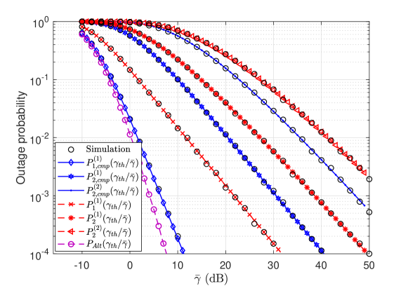
Figure 1: Outage probability vs average SNR for $\gamma_{\text{th}}=0$ dB.

Figure 2 compares the throughput in nats/sec/Hz as a function of $\bar{\gamma}$ (in dB) in the presence and absence of the RIS. A good agreement between the analytical and simulation results can be observed, and the improvement of the throughput due to the phase compensation at the RIS is clearly visible in the figure. Again, for comparison, the throughput $R_{\text{Alt}}$ corresponding to the above numerically optimized scheme is also plotted. As depicted in the figure, the proposed scheme provides a very tight lower bound to the optimal throughput. This claim further highlights the utility of the proposed scheme.

Figure 2: Average throughput vs average SNR.

V Conclusion

We have analytically characterized the exact outage and throughput of a two-tile RIS-assisted $2\times 2$ wireless network in the presence of Rayleigh fading. In particular, we have considered transmission strategies corresponding to all combinations of left and right singular spaces of the RIS-receiver and transmit-RIS channels that are optimal in terms of the average SNR. It turns out that, although sub-optimal, the proposed strategy has outage and throughput performances comparable with the numerically jointly optimized scheme. In particular, with respect to throughput, the proposed scheme provides a tight lower bound to the numerically optimal scheme. Moreover, we have proved that the average SNR improves of about 2 dB thanks to the phase compensation introduced by the RIS.

Appendix A

To facilitate our main derivations, we will require the following preliminary result.

Lemma 5.

Let $\mathbf{S}\in\mathcal{U}_{2}$. Then $\mathbf{S}$ can be parameterized as [20]

$$\mathbf{S}=\left(\begin{array}[]{cr}e^{j\theta_{11}}\cos\theta_{12}&-e^{j\left(\theta_{11}+\theta_{21}\right)}\sin\theta_{12}\\ e^{j\theta_{22}}\sin\theta_{12}&e^{j\left(\theta_{22}+\theta_{21}\right)}\cos\theta_{12}\end{array}\right)$$

where $\theta_{ij}\in[0,2\pi)$ for $i\geq j$ and $\theta_{12}\in[0,\pi/2]$. Moreover, if $\mathbf{S}$ is uniformly distributed over $\mathcal{U}_{2}$, then all the entries of $\mathbf{S}$ are identically distributed and the normalized invariant measure ${\rm d}\mathbf{S}$ (i.e, Haar measure) defined on $\mathcal{U}_{2}$ such that $\int_{\mathcal{U}_{2}}{\rm d}\mathbf{S}=1$ is given by [20]

$$\mathrm{d}\mathbf{S}=\frac{1}{8\pi^{3}}\sin 2\theta_{12}{\rm d}\theta_{12}{\rm d}\theta_{21}{\rm d}\theta_{11}{\rm d}\theta_{22}.$$

Therefore, the random variables $\theta_{ij}$ are independent for $i,j=1,2$ with their densities given by $f_{\theta_{12}}(\theta)=\sin 2\theta,\;\;\;0\leq\theta\leq\pi/2,$ and $\theta_{ij}\sim\text{Uniform}(0,2\pi),\;\;\;j\leq i.$

A-A Proof of Theorem 1

Since the column spaces of $\mathbf{U}$ and $\mathbf{Q}$ form orthonormal bases, we can find $\bm{\alpha},\bm{\beta}\in\mathbb{C}^{2\times 1}$ such that $\mathbf{b}=\mathbf{U}\bm{\alpha}$ and $\mathbf{a}=\mathbf{Q}\bm{\beta}$ with $||\bm{\alpha}||^{2}=||\bm{\beta}||^{2}=1$. If we denote $\bm{\alpha}=\left(\alpha_{1}\;\alpha_{2}\right)^{T}$ and $\bm{\beta}=\left(\beta_{1}\;\beta_{2}\right)^{T}$, then (2) can be written as

$$\gamma=\bar{\gamma}\sum_{k,\ell,i,j=1}^{2}\sqrt{\lambda_{k}\omega_{\ell}\lambda_{i}\omega_{j}}\alpha_{k}^{*}\alpha_{i}\beta_{l}\beta_{j}^{*}\text{Tr}\left(\mathbf{v}_{i}\mathbf{v}_{k}^{\dagger}\bm{\Phi}\mathbf{w}_{\ell}\mathbf{w}_{j}^{\dagger}\bm{\Phi}^{\dagger}\right).$$

Capitalizing on the independence between the singular values and singular vectors [16] and noting that, under the assumption that $\bf\Phi$ is a constant matrix that is not optimized and is independent of the wireless channels, the distributions of $\bm{\Phi}\mathbf{w}_{\ell}$ and $\bm{\mathbf{w}_{j}^{\dagger}\Phi}^{\dagger}$ are the same as $\mathbf{w}_{\ell}$ and $\mathbf{w}_{j}$, we obtain

$$\mathbb{E}\left\{\gamma\right\} =\bar{\gamma}\sum_{k,\ell,i,j=1}^{2}\alpha_{k}^{*}\alpha_{i}\beta_{\ell}\beta_{j}^{*}\mathbb{E}\left\{\sqrt{\lambda_{k}\omega_{\ell}\lambda_{i}\omega_{j}}\right\}\text{Tr}\left(\mathbb{E}\left\{\mathbf{v}_{i}\mathbf{v}_{k}^{\dagger}\right\}\mathbb{E}\left\{\mathbf{w}_{\ell}\mathbf{w}_{j}^{\dagger}\right\}\right).$$ (A.1)

In order to evaluate the expected values inside the trace operator, following Lemma 5, we parameterize the matrices $\mathbf{V}$ and $\mathbf{W}$ to yield

$$\mathbf{V}=\left(\begin{array}[]{cr}e^{j\xi_{11}}\cos\xi_{12}&-e^{j\left(\xi_{11}+\xi_{21}\right)}\sin\xi_{12}\\ e^{j\xi_{22}}\sin\xi_{12}&e^{j\left(\xi_{22}+\xi_{21}\right)}\cos\xi_{12}\end{array}\right),$$

and

$$\mathbf{W}=\left(\begin{array}[]{cr}e^{j\psi_{11}}\cos\psi_{12}&-e^{j\left(\psi_{11}+\psi_{21}\right)}\sin\psi_{12}\\ e^{j\psi_{22}}\sin\psi_{12}&e^{j\left(\psi_{22}+\psi_{21}\right)}\cos\psi_{12}\end{array}\right),$$

where $\xi_{ij},\psi_{ij}\in[0,2\pi)$ for $i\geq j$ and $\xi_{12},\psi_{12}\in[0,\pi/2]$. Moreover, since $\mathbf{V}$ and $\mathbf{W}$ are uniformly and independently distributed over $\mathcal{U}_{2}$ [16], $\xi_{ij}$ and $\psi_{ij}$ are independent and identically distributed (i.i.d.)[20]. Therefore, we obtain

$$\mathbb{E}\left\{\mathbf{v}_{i}\mathbf{v}_{k}^{\dagger}\right\}=\left\{\begin{array}[]{cc}\frac{1}{2}\mathbf{I}_{2}&\text{if $i=k$}\\ \mathbf{0}&\text{if $i\neq k$}\end{array}\right.$$

and

$$\mathbb{E}\left\{\mathbf{w}_{\ell}\mathbf{w}_{j}^{\dagger}\right\}=\left\{\begin{array}[]{cc}\frac{1}{2}\mathbf{I}_{2}&\text{if $j=\ell$}\\ \mathbf{0}&\text{if $j\neq\ell$}\end{array}\right..$$

Then, (A.1) gives

$$\mathbb{E}\left\{\gamma\right\}=\frac{\bar{\gamma}}{2}\bm{\alpha}^{\dagger}\left(\begin{array}[]{cc}\mathbb{E}\{\lambda_{1}\}&0\\ 0&\mathbb{E}\{\lambda_{2}\}\end{array}\right)\bm{\alpha}\bm{\beta}^{\dagger}\left(\begin{array}[]{cc}\mathbb{E}\{\omega_{1}\}&0\\ 0&\mathbb{E}\{\omega_{2}\}\end{array}\right)\bm{\beta}$$

where $\mathbb{E}\{\lambda_{1}\}>\mathbb{E}\{\lambda_{2}\}$ and $\mathbb{E}\{\omega_{1}\}>\mathbb{E}\{\omega_{2}\}$. Clearly, $\bm{\alpha}=e^{j\chi_{1}}\left(1\;0\right)^{T}$ and $\bm{\beta}=e^{j\chi_{2}}\left(1\;0\right)^{T}$, with $\chi_{1},\chi_{2}\in[0,2\pi)$ denoting arbitrary phases, simultaneously maximize $\mathbb{E}\{\gamma\}$ subject to the constraints $||\bm{\alpha}||^{2}=||\bm{\beta}||^{2}=1$. Therefore, we conclude that the pair $(\mathbf{a},\mathbf{b})\equiv\left(\mathbf{q}_{1},\mathbf{u}_{1}\right)$ is optimal in the sense of maximizing the average SNR. Similar arguments can be used to establish that $(\mathbf{a},\mathbf{b})\equiv(\mathbf{q}_{2},\mathbf{u}_{2})$ corresponds to the minimum average SNR.

Having noted that $\gamma_{j}^{(i)}=\bar{\gamma}\lambda_{j}\omega_{i}\text{Tr}\left(\mathbf{v}_{j}\mathbf{v}_{j}^{\dagger}\bm{\Phi}\mathbf{w}_{i}\mathbf{w}_{i}^{\dagger}\bm{\Phi}^{\dagger}\right)$ and $\mathbb{E}\left\{\text{Tr}\left(\mathbf{v}_{j}\mathbf{v}_{j}^{\dagger}\bm{\Phi}\mathbf{w}_{i}\mathbf{w}_{i}^{\dagger}\bm{\Phi}^{\dagger}\right)\right\}=\frac{1}{2},$ we obtain $\mathbb{E}\left\{\gamma_{j}^{(i)}\right\}=\frac{\bar{\gamma}}{2}\mathbb{E}\{\lambda_{j}\}\mathbb{E}\{\omega_{i}\}$. Finally, we use the inequalities

$$\lambda_{1}\omega_{1}>\lambda_{1}\omega_{2}>\lambda_{2}\omega_{2}\quad\text{and}\quad\lambda_{1}\omega_{1}>\lambda_{2}\omega_{1}>\lambda_{2}\omega_{2},$$ (A.2)

along with the fact that $\mathbb{E}\{\lambda_{1}\}\mathbb{E}\{\omega_{2}\}=\mathbb{E}\{\lambda_{2}\}\mathbb{E}\{\omega_{1}\}$ to obtain (3) which concludes the proof.

A-B Proof of Corollary 2

Following the above parametatrizations of unitary matrices, we can rewrite (5) as $\gamma_{i,\text{comp}}^{(i)}=\bar{\gamma}\lambda_{i}\omega_{i}\cos^{2}\left(\xi_{12}-\psi_{12}\right),\;\;i=1,2$ and $\gamma_{j,\text{comp}}^{(i)}=\bar{\gamma}\lambda_{j}\omega_{i}\sin^{2}\left(\xi_{12}+\psi_{12}\right),\;\;i\neq j.$

Since $\mathbb{E}\left\{\cos^{2}\left(\xi_{12}-\psi_{12}\right)\right\}=\mathbb{E}\left\{\sin^{2}\left(\xi_{12}+\psi_{12}\right)\right\},$ we use the inequalities (A.2) and the relation $\mathbb{E}\{\lambda_{1}\}\mathbb{E}\{\omega_{2}\}=\mathbb{E}\{\lambda_{2}\}\mathbb{E}\{\omega_{1}\}$ to obtain (6). This concludes the proof.

A-C Proof of Theorem 3

The unitary matrix parameterizations given in (A-A) yields

$$Z_{j,\text{cmp}}^{(i)}=\left\{\begin{array}[]{cc}\cos^{2}\left(\xi_{12}-\psi_{12}\right)&\text{for $i=j$}\\ \sin^{2}\left(\xi_{12}+\psi_{12}\right)&\text{for $i\neq j$}\end{array}\right.$$ (A.5)

where the distributions of $\xi_{12}$ and $\psi_{12}$ are i.i.d. with the common density $f(\theta)=\sin 2\theta,\;\;\theta\in[0,\pi/2]$ [20]. Therefore, simple variable transformations yield

$$f_{\left(\xi_{12}-\psi_{12}\right)}(x)=\frac{1}{2}\left(\frac{\pi}{2}\cos 2x-|x|\cos 2x+\frac{1}{2}\sin 2|x|\right),\;\;x\in[-\pi/2,\pi/2]$$

and

$$f_{\xi_{12}+\psi_{12}}(x)=\left\{\begin{array}[]{lc}\frac{1}{4}\sin 2x-\frac{x}{2}\cos 2x&\text{for $x\in\left[0,\frac{\pi}{2}\right)$}\\ -\frac{1}{4}\sin 2x-\frac{(\pi-x)}{2}\cos 2x&\text{for $x\in\left[\frac{\pi}{2},\pi\right]$}.\end{array}\right.$$

Since we are interested in the c.d.f.s, we can use integration by parts followed by algebraic manipulations to obtain (7).

Let us now focus on proving (8). To this end, noting that the distribution of $|\mathbf{v}_{j}^{\dagger}\bm{\Phi}\mathbf{w}_{i}|^{2}$ is independent of the indices $i,j$ [20], we focus on the case $i=j=1$. We compute the Laplace transform to obtain the moment generating function (m.g.f.) as

$$\mathcal{M}(s)=\mathbb{E}\left\{\exp\left(-\text{Tr}\left[\bm{\Theta}\mathbf{V}^{\dagger}\bm{\Phi}\mathbf{w}_{1}\mathbf{w}_{1}^{\dagger}\bm{\Phi}^{\dagger}\mathbf{V}\right]\right)\right\}$$

where $\bm{\Theta}=\text{diag}\left(s,0\right)$, and the expected value is taken with respect to the product measure ${\rm d}\mathbf{V}{\rm d}\mathbf{W}$ where ${\rm d}\mathbf{V}$ and ${\rm d}\mathbf{W}$ are independent and Haar distributed. Therefore, by exploiting the independence between $\mathbf{V}$ and $\mathbf{W}$, we rewrite the m.g.f. as

$$\mathcal{M}(s)=\mathbb{E}_{\mathbf{W}}\left\{\int_{\mathcal{U}(2)}\exp\left(-\text{Tr}\left[\bm{\Theta}\mathbf{V}^{\dagger}\bm{\Phi}\mathbf{w}_{1}\mathbf{w}_{1}^{\dagger}\bm{\Phi}^{\dagger}\mathbf{V}\right]\right){\rm d}\mathbf{V}\right\},$$

where $\mathbb{E}_{\mathbf{W}}(\cdot)$ stands for the expected value with respect to the Haar measure ${\rm d}\mathbf{W}$. Then, we use [17, Eq. 89] to simplify the inner matrix integral to obtain

$$\mathcal{M}(s)=\mathbb{E}_{\mathbf{W}}\left\{{}_{0}\mathcal{F}_{0}\left(-\bm{\Theta},\bm{\Phi}\mathbf{w}_{1}\mathbf{w}_{1}^{\dagger}\bm{\Phi}^{\dagger}\right)\right\}$$

where ${}_{0}\mathcal{F}_{0}(\cdot,\cdot)$ is the hypergeometric function of two matrix arguments. We expand the hypergeometric function as an infinite series to yield [17]

$$\mathcal{M}(s)=\mathbb{E}_{\mathbf{W}}\left\{\sum_{k=0}^{\infty}\frac{(-1)^{k}}{k!}\sum_{\kappa}\frac{C_{\kappa}(\bm{\Theta})C_{\kappa}(\bm{\Phi}\mathbf{w}_{1}\mathbf{w}_{1}^{\dagger}\bm{\Phi}^{\dagger})}{C_{\kappa}(\mathbf{I}_{2})}\right\}$$

where $C_{\kappa}(\cdot)$ denotes the zonal polynomial corresponding to the partition $\kappa=(\kappa_{1},\kappa_{2})$ with $\kappa_{1}\geq\kappa_{2}\geq 0$ and $\kappa_{1}+\kappa_{2}=k$. Since the matrices $\bm{\Theta}$ and $\bm{\Phi}\mathbf{w}_{1}\mathbf{w}_{1}^{\dagger}\bm{\Phi}^{\dagger}$ have rank one, applying the complex analogue of [21, Corollary 7.2.4], we obtain $C_{\kappa}(\bm{\Theta})=\text{Tr}^{k}(\bm{\Theta})=s$ and $C_{\kappa}\left(\bm{\Phi}\mathbf{w}_{1}\mathbf{w}_{1}^{\dagger}\bm{\Phi}^{\dagger}\right)=\text{Tr}^{k}\left(\bm{\Phi}\mathbf{w}_{1}\mathbf{w}_{1}^{\dagger}\bm{\Phi}^{\dagger}\right)=1$. Therefore, we obtain

$$\mathcal{M}(s)=\mathbb{E}_{\mathbf{W}}\left\{\sum_{k=0}^{\infty}\frac{(-s)^{k}(1)_{k}}{k!(2)_{k}}\right\}={}_{1}F_{1}(1;2;-s)$$

where ${}_{1}F_{1}(\cdot;\cdot;\cdot)$ denotes the confluent hypergeometric function of the first kind [18] and we have used the fact that $C_{k}\left(\mathbf{I}_{2}\right)=(2)_{k}/(1)_{k}$ with $(a)_{k}=a(a+1)\cdots(a+k-1)$ denoting the Pochhammer symbol. Finally, using [18, Eq. 9.211.2], we obtain

$$\mathcal{M}(s)=\int_{0}^{1}\exp(-st){\rm d}t$$ (A.6)

from which it can be concluded that the random variable $|\mathbf{v}_{1}^{\dagger}\bm{\Phi}\mathbf{w}_{1}|^{2}$ is uniformly distributed over $[0,1]$.

References

• [1] M. D. Renzo et al., “Smart radio environments empowered by AI reconfigurable meta-surfaces: An idea whose time has come,” EURASIP J. Wireless Commun. Netw., vol. 2019:129, May 2019.
• [2] Q. Wu and R. Zhang, “Intelligent reflecting surface enhanced wireless network via joint active and passive beamforming,” IEEE Trans. Wireless Commun., vol. 18, no. 11, pp. 5394–5409, 2019.
• [3] A. Zappone et al., “Overhead-aware design of reconfigurable intelligent surfaces in smart radio environments,” IEEE Trans. Wireless Commun., 2020, Early Access Article.
• [4] M. D. Renzo et al., “Smart radio environments empowered by reconfigurable intelligent surfaces: How it works, state of research, and road ahead,” IEEE J. Select. Areas Commun., 2020, Early Access Article.
• [5] Y. Han et al., “Large intelligent surface-assisted wireless communication exploiting statistical CSI,” IEEE Trans. Veh. Technol., vol. 68, no. 8, pp. 8238–8242, Aug. 2019.
• [6] Q. Nadeem et al., “Asymptotic max-min SINR analysis of reconfigurable intelligent surface assisted MISO systems,” IEEE Trans. Wireless Commun., 2020, Early Access Article.
• [7] M. Jung et al., “Performance analysis of large intelligent surfaces (LISs): Asymptotic data rate and channel hardening effects,” IEEE Trans. Wireless Commun., vol. 19, no. 3, pp. 2052–2065, 2020.
• [8] W. Zhao et al., “Performance analysis of large intelligent surface aided backscatter communication systems,” IEEE Wireless Commun. Lett., vol. 9, no. 7, pp. 962–966, 2020.
• [9] S. Atapattu et al., “Reconfigurable intelligent surface assisted two–way communications: Performance analysis and optimization,” IEEE Trans. Commun., 2020, Early Access Article.
• [10] H. Zhang, et al., “Reconfigurable intelligent surfaces assisted communications with limited phase shifts: How many phase shifts are enough?” IEEE Trans. Veh. Technol., vol. 69, no. 4, pp. 4498–4502, 2020.
• [11] B. Di, et al., “Hybrid beamforming for reconfigurable intelligent surface based multi-user communications: Achievable rates with limited discrete phase shifts,” IEEE J. Select. Areas Commun., vol. 38, no. 8, pp. 1809–1822, 2020.
• [12] X. Qian et al., “Beamforming through reconfigurable intelligent surfaces in single-user MIMO systems: SNR distribution and scaling laws in the presence of channel fading and phase noise,” IEEE Wireless Commun. Lett., 2020, Early Access Article.
• [13] M. Najafi et al., “Physics-based modeling and scalable optimization of large intelligent reflecting surfaces,” https://arxiv.org/abs/2004.12957, 2020.
• [14] L. D. Chamain, et al., “Eigenvalue-based detection of a signal in colored noise: Finite and asymptotic analyses,” IEEE Trans. Inform. Theory, vol. 66, no. 10, pp. 6413–6433, 2020.
• [15] F. H. Danufane et al., “On the path-loss of reconfigurable intelligent surfaces: An approach based on Green’s theorem applied to vector fields,” Available: https://arxiv.org/abs/2007.13158.
• [16] J. Shen, “On the singular values of Gaussian random matrices,” Linear Algebra Appl., vol. 326, no. 1-3, pp. 1–14, Mar. 2001.
• [17] A. T. James, “Distributions of matrix variates and latent roots derived from normal samples,” Ann. Math. Statist., vol. 35, no. 2, pp. 475–501, Jun. 1964.
• [18] I. S. Gradshteyn and I. M. Ryzhik, Table of Integrals, Series and Products, 7th ed.   Academic Press Inc, 2007.
• [19] D. Bertsekas, Nonlinear Programming, ser. Athena scientific optimization and computation series.   Athena Scientific, 1999.
• [20] C. Spengler, M. Huber, and B. C. Hiesmayr, “Composite parameterization and Haar measure for all unitary and special unitary groups,” J. Math. Phys, vol. 53, no. 1, p. 013501, Jan. 2012.
• [21] R. J. Muirhead, Aspects of Multivariate Statistical Theory.   Wiley-Interscience, 2005.