NGC 7538 IRS1 - an O star driving an ionized jet and giant N-S outflow

Abstract

NGC 7538 IRS 1 is a very young embedded O star driving an ionized jet and accreting mass with an accretion rate $>$10^-4  M_⊙/year, which is quenching the hypercompact H II region. We use SOFIA GREAT data, Herschel PACS and SPIRE archive data, SOFIA FORCAST archive data, Onsala 20m and CARMA data, and JCMT archive data to determine the properties of the O star and its outflow. IRS 1 appears to be a single O-star with a bolometric luminosity $>$ 1 $\times$ 10⁵  L_⊙, i.e. spectral type O7 or earlier. We find that IRS 1 drives a large molecular outflow with the blue-shifted northern outflow lobe extending to $\sim$ 280^′′ or 3.6 pc from IRS 1. Near IRS 1 the outflow is well aligned with the ionized jet. The dynamical time scale of the outflow is $\sim$ 1.3 $\times$ 10⁵ yr. The total outflow mass is $\sim$ 130  M_⊙. We determine a mass outflow rate of 1.0 $\times$10^-3  M_⊙yr^-1, roughly consistent with the observed mass accretion rate. We observe strong high velocity [C ii] emission in the outflow, confirming that strong UV radiation from IRS 1 escapes into the outflow lobes and is ionizing the gas. Many O stars may form like low mass stars, but with a higher accretion rate and in a denser environment. As long as the accretion stays high enough to quench the H II region, the star will continue to grow. When the accretion rate drops, the H II region will rapidly start to expand.

1. Introduction

The molecular cloud south of the H II region NGC 7538 harbors several young massive stars, of which at least three, IRS 1, IRS 9 and NGC 7538 S, are centers of young clusters. At a distance of 2.65 kpc (Moscadelli et al., 2008) NGC 7538 is by no means the closest high-mass star forming region, but the extreme youth of these stars make them key targets for our understanding of high mass star formation. NGC 7538 IRS 1 was first detected as an OH maser by Hardebeck (1971) indicating that there is another H II region SE of the optically visible H II region NGC 7538. It was first detected in the radio at 5 GHz by Martin (1973), who found three compact radio sources at the SE edge of the compact ($\sim$ 4^′) H II region NGC 7538. The brightest of the three, i.e., Martin’s source B, is commonly referred to as NGC 7538 IRS 1, based on near/mid-IR high spatial resolution mapping and photometry by (Wynn-Williams, Becklin, & Neugebauer, 1974). In addition to the radio sources IRS 1 – 3, Qiu, Zhang & Menten (2011) also found 8 cores at 1.3 mm using the Submillimeter Array (SMA) within a projected distance of 0.35 pc from IRS 1, many of which are associated with H₂O maser emission or outflow activity suggesting they are young pre-main-sequence stars. Frau et al. (2014) increased the number of cores to 13 by more sensitive observations with the SMA at 880 $\mu$m. IRS 1 is the most massive star in a cluster with more than 150 Young Stellar Objects (YSOs) and protostars (Mallick et al., 2014; Sharma et al., 2017).

The radio emission from IRS 1 was first resolved with the Karl G. Jansky Very Large Array (VLA) at 14.9 GHz by Campbell (1984), who showed that the radio emission consists of a compact ($\sim$0$\farcs$2) bipolar N-S core with faint extended fan shaped lobes, suggesting an ionized outflow. High angular resolution observations of radio recombination lines (Gaume et al., 1995; Sewilo et al., 2004; Keto et al., 2008) revealed extremely broad lines indicating substantial mass motion of the ionized gas. Keto et al. (2008) modeled the spectral energy distribution (SED) of IRS 1 as a combination of two H II regions plus dust, which could adequately fit the data available at the time. However, Sandell et al. (2009), who analyzed high angular resolution VLA archive data from 4.86 GHz to 43.4 GHz found that the bipolar core had a spectral index of $\sim$ 0.8 and that the size of the core shrank as a function of frequency with a power law index of $\sim$ - 0.8, which is what one would expect from an ionized jet (e.g., Reynolds, 1986), but not from an optically thick H II region. It is therefore clear that IRS 1 drives a bipolar ionized jet.

IRS 1 is heavily accreting with an accretion rate of $\sim$10^-3 - 2 10^-4 M_⊙/yr (Sandell et al., 2009; Klaassen et al., 2011; Qiu, Zhang & Menten, 2011; Beuther, Linz & Henning, 2012; Zhu et al., 2013), which quenches the expansion of an H II region. IRS 1 itself is an extremely rich maser source, with not only just the normal masers found in high mass stars like OH, H₂O, and CH₃OH, but also rare masers like NH₃, H₂CO, and the 23.1 GHz class II CH₃OH maser. The latter has to date been only detected in three sources, see Gálvan-Madrid et al. (2010) and references therein. These masers are most likely pumped by the radio emission from the jet. IRS 1 is almost certainly surrounded by an accretion disk, but so far there is no firm evidence for a Keplerian accretion disk surrounding IRS 1. The orientation of the linear polarization of the 157 GHz CH3OH class II maser towards IRS 1 agrees with that of the submillimeter dust polarization, suggesting a magnetic field oriented along the outflow axis (Wiesemeyer, Thum & Walmsley, 2004). The same holds for the 133 GHz class I maser, residing 40^′′ south of IRS 1 and possibly associated with a bow-shock in the red-shifted outflow lobe. While it is unclear whether the 157 GHz maser originates from an accretion disk or from the outflow. There have been many claims that IRS 1 is surrounded by an accretion disk in Keplerian rotation (Minier, Booth & Conway, 1998, 2000; Pestalozzi et al., 2004; Pestalozzi, Elitzur & Conway, 2009; Surcis et al., 2011; Moscadelli & Goddi, 2014) based on linear methanol maser features. Moscadelli & Goddi (2014) identified three maser groups and suggested that IRS 1 is a triple system, where each high mass YSO in the system is surrounded by an accretion disk and probably drives an outflow. Beuther et al. (2017), who imaged IRS 1 at 23 GHz with the VLA in the A configuration, identified two of these maser features being close to peaks in the free-free emission, and argued that IRS 1 is a binary, powered by two hypercompact H II regions, each with a spectral index of 1.5 - 2. This does not agree with the observed spectral index of IRS 1 and with high angular (CARMA) A-array data analyzed in this paper. Here we will therefore re-examine whether IRS 1 is a single star or a multiple system.

Scoville et al. (1986) using the Owens Valley Radio Observatory (OVRO) millimeter array at 2.7 mm was the first to positively identify the high velocity CO(1-0) emission seen toward NGC 7538 as a bipolar outflow powered by IRS 1 with the outflow at a position angle (PA) of 145^∘ (counterclockwise against north), being red-shifted in the SE and blue-shifted to the NW with a total extent of $\sim$ 3^′, i.e., 2.3 pc. This agrees well with other studies (Fischer et al., 1985; Kameya et al., 1989; Davis et al., 1998). However, if this is the case, the ionized jet and the molecular outflow are misaligned. This led (Kraus et al., 2006) to interpret mid-IR speckle images as a precessing jet where IRS 1 would undergo non-coplanar tidal interaction with an undiscovered close companion within the circumbinary protostellar disk. Sandell et al. (2012) presented single dish James Clerk Maxwell Telescope (JCMT) CO(3–2) data, which show blue-shifted high-velocity gas $\sim$80^′′ north of IRS 1, which suggested that the molecular outflow is quite large and well aligned with the ionized outflow. Here we present an extended CO(3–2) map from JCMT, as well as [C ii] 158 $\mu$m and high-J CO data obtained with GREAT on the Stratospheric Observatory for Infrared Astronomy (SOFIA). Analysis of these new data sets conclusively show that IRS 1 drives a large N-S molecular and ionized outflow.

2. Observations

2.1. GREAT observations

The NGC 7538 IRS 1 outflow was observed in the GREAT L1/L2 configuration (Heyminck et al., 2012) on SOFIA (Young et al., 2012) on January 23, 2015 as part of the open time project 02_0038. These observations were done on a 44 minute leg at 41300 feet. The L2 mixer was tuned to the [C ii] ${}^{2}{\rm P}_{3/2}\to\ ^{2}{\rm P}_{1/2}$ transition at 1.9005369 THz , while the L1 mixer was tuned to CO(11–10) at a rest frequency of 1.26701449 THz. The main beam coupling efficiency, $\eta_{mb}$ = 0.69 for L2, and 0.65 for L1. The Half Power Beam Width (HPBW) for L2 was measured to be 14$\farcs$1 for [C ii] and 21$\farcs$1 for CO(11-10). These observations were complemented with observations on May 20, and 21, 2015 during the Low Frequency Array (LFA) commissioning. The LFA array is a hexagonal array with two polarizations co-aligned around a central pixel, providing a 2 $\times$ 7 pixel array with the pixels separated by two beam widths. For a more complete description of the instrument, see Risacher et al. (2016). The LFA receiver was tuned to [C ii], while the second channel, L1, was tuned to CO(11–10). The measured HPBW for LFA was 15${}^{\prime\prime}\mskip-7.6mu.\,$1 and the main beam coupling efficiency, $\eta_{mb}$ = 0.69, while the HPBW for L1 was 21$\farcs$1 and $\eta_{mb}$ = 0.64. On May 20, we had a 50 minute leg at 45,000 ft. On May 21 the leg duration was 52 minutes at 43,000 ft. The precipitable water vapor was $\leq$ 9 $\mu$m on both nights. In January 2015 (L1/L2) we did an OTF TP map with a size of 82${}^{\prime\prime}\mskip-7.6mu.\,$5 $\times$ 97${}^{\prime\prime}\mskip-7.6mu.\,$5 scanning in RA with 7${}^{\prime\prime}\mskip-7.6mu.\,$5 sampling and an integration time of 2 second/point. The off position was at +600^′′,0^′′relative to IRS 1. We also took a 10 minute pointed integration on IRS 1. In May 2015 we did much larger maps with upGREAT. These were done in classic on-the-fly (OTF) total power (TP) mode, with scanning in RA with a 7^′′ sampling and an integration time of 2 second/point using the same off position. The final map size in [C ii] is $\sim$ 160^′′ $\times$ 240^′′. For CO(11–1) the map size is 105^′′ $\times$ 196^′′. All the data were added together in the post processing.

The backends for both GREAT channels are the latest generation of fast Fourier transform spectrometers (FFTS) (Klein et al., 2012). These have 4 GHz bandwidth and 16384 channels, which provide a channel separation of 244.1 kHz (0.0385 km s^-1 for [C ii]). The data were reduced and calibrated by the GREAT team. The post processing was done using CLASS. We removed linear baselines, threw away a few damaged spectra and created maps with rms weighting.

Table 1Positions and flux densities of FORCAST mid-infrared sources. Errors are one sigma statistical errors.

Source	$\alpha$(2000.0)	$\delta$(2000.0)	S(7.7 $\mu$m)	S(19.7$\mu$m)	S(25.3 $\mu$m)	S(31.5 $\mu$m)	S(37.0 $\mu$m)
	[h m s]	[∘ ′ ′′]	[Jy]	[Jy]	[Jy]	[Jy]	[Jy]
IRS 1	23 13 45.37	+61 28 10.5	170.7 $\pm$ 3.3	240 $\pm$ 8.1	787 $\pm$ 30	1320 $\pm$ 28.2	1710 $\pm$ 50
IRS 2	23 13 45.44	+61 28 20.1	9.4 $\pm$ 5.0	508 $\pm$ 16.2	360 $\pm$ 70	550 $\pm$ 30.0	540 $\pm$ 90
IRS 3	23 13 43.62	+61 28.14.2	2.9 $\pm$ 0.2	85 $\pm$ 6.0	166 $\pm$ 17	223 $\pm$ 12.5	249 $\pm$ 25
IRS 4	23 13 32.39	+61 29 06.2	5.2 $\pm$ 0.3	$\cdots$	$\cdots$	41.8 $\pm$ 0.6	32 $\pm$ 0.8
IRS 1E	23 13 48.64	+61 28 05.1	0.46 $\pm$ 0.10	1.49 $\pm$ 0.20	5.4 $\pm$ 0.6	5.3 $\pm$ 0.5	6.6 $\pm$ 2.1
IRS 1SE	23 13 48.40	+61 27 40.3	$<$ 0.5	1.11 $\pm$ 0.10	3.3 $\pm$ 0.5	3.6 $\pm$ 0.5	1.2 $\pm$ 0.8

2.2. CARMA observations

Observations at 1.3 mm were obtained in the A configuration on December 6, 2011 using 16 500 MHz bandwidth spectral windows, and on December 7, 2011 using 14 500 MHz windows and two 125 MHz windows which covered the H30$\alpha$ recombination line with $\sim$ 1 km s^-1 spectral resolution. The data were calibrated using the calibration sources J0102$+$584, 3C 454.3 and MWC 349 in a standard way using the Miriad software package (Sault et al., 1995). Due to hardware and software limitations in the 2nd and 3rd local oscillator phase tracking for the wide band correlator during these commissioning observations in the A configuration, the phase tracking center was offset in each spectral window. Apart from the offset, the images in each spectral window agreed within the noise, and we used a shift and add procedure (using the Miriad tasks IMDIFF and AVMATHS) to average the 500 MHz spectral windows. The December 7 2011 data were self calibrated using the strong H30$\alpha$ emission. The December 6 2011 data used the continuum emission in the same spectral window in a 500 MHz bandwidth. The continuum images at 227.4 GHz obtained from the two data sets are consistent.

CARMA A-array observations were also obtained at 111.1 GHz on December 10, and 12, 2011, and in the B-array configuration on January 3 – 4, and January 5 – 6, 2012. B-array observations were also obtained at 222.2 GHz on January 2 and 3, 2012. All these observations used the same backend configuration as described above. These data sets were reduced in Miriad following the same procedure described in Zhu et al. (2013).

We also retrieved some mosaicked CARMA ¹²CO(1–0) and ¹³CO(1–0) images, which allows us to get a better look of the outflow close to IRS 1. The observations and data reduction of these data sets are described in Corder (2008). In particular we use a ¹²CO(1–0) image with 4${}^{\prime\prime}\mskip-7.6mu.\,$5 angular resolution and a velocity resolution of 1.27 km s^-1. This image has a root mean square sensitivity of 0.64 K per channel. The total velocity coverage of the ¹²CO is from -96 km s^-1 – -16 km s^-1. We also retrieved a ¹³CO(1–0) image made from the C and D array configurations resulting in a resolution of 7${}^{\prime\prime}\mskip-7.6mu.\,$9 $\times$ 7${}^{\prime\prime}\mskip-7.6mu.\,$4 PA = 55 degr. We corrected this image for missing zero spacing by adding the ¹³CO(1–0) OSO map to this image using the MIRIAD task IMMERGE. The velocity resolution of this map is 0.33 km s^-1 and it covers the velocity range from -65.8 km s^-1– -45.8 km s^-1.

2.3. CO(1-0) and ¹³CO(1-0) mapping with the 20 m Onsala Space Telescope

We observed the NGC 7538 molecular cloud in CO(1–0) and ¹³CO(1–0) with an SIS mixer on the 20 m Onsala Space telescope in Sweden from January 28 to February 4 2010. The backend was a 1600-channel hybrid digital autocorrelator spectrometer with 50 kHz resolution. The beam size is 33^′′ and 34^′′ for ¹²CO and ¹³CO, respectively. The main beam efficiency is elevation dependent, but for the bulk of the data it was $\sim$0.42 for CO and 0.45 for ¹³CO. All observations were done in Total Power position switch mode. We mapped the cloud on a regular grid with a 15^′ spacing using an integration time of 3 minute/position. In total we mapped an area of 240^′′ $\times$ 300^′′ in CO(1–0) and 400^′′ $\times$ 380^′′ in ¹³CO(1–0). Both maps were centered on IRS 1. The weather was generally quite good, although some time was lost due to heavy snowfall. The system temperature for the ¹³CO setting was typically between 250 - 350 K going up to about twice that much for ¹²CO. All the data reduction was done in CLASS. We removed low order baselines and occasionally standing waves. The spectra were then coadded with RMS weighting. The final maps were exported as FITS cubes and imported into MIRIAD for further analysis.

2.4. JCMT archive data

We obtained a fully sampled CO(3–2) map from C. Fallscheer covering a 1^∘ $\times$ 1^∘ region of NGC 7538. This map was observed with the Heterodyne Array Receiver Program (HARP; Buckle et al. (2009)) on the JCMT at Maunakea, Hawaii. HARP has a beamsize of 14${}^{\prime\prime}\mskip-7.6mu.\,$6 at 345.8 GHz and the main beam efficiency is 0.63. The reduction of the CO(3–2) data is described in Fallscheer et al. (2013). The CO data cube covers a 1 GHz wide band with 2048 channels, providing a velocity resolution of 0.42 km s^-1 per channel. The 1$\sigma$ rms per channel is $\sim$0.8 K on the T_mb scale. Here we only use part of the map covering the H II region and the molecular cloud southwest of it.

We also got two long integration HARP maps done in position switched jiggle mode from Jan Wouterloot covering $\sim$ 100^′′ $\times$ 100^′′, one in ¹²CO(3–2) and one of ¹³CO(3–2). Both maps have a bandwidth of 1000 MHz, i.e., a frequency resolution of 488.3 kHz, which for ¹²CO corresponds to a velocity resolution of 0.42 km s^-1. The ¹²CO map is a coadd of 22 observations, which were all of good quality, while the ¹³CO is based on 6 independent observations. The final averages were re-gridded onto a 30^′′ grid. The rms noise per channel is 30 mK for CO(3–2) and 40 mK for ¹³CO(3–2) respectively.

Figure 1.— Three-color image of the IRS 1 – 3 region generated by combining the FORCAST 19 (blue), 25 (green), and 37 $\mu$m (red) images in logarithmic scale. IRS 1 is the strong yellow source at offset 0^′′, 0^′′. IRS 2 at 0${}^{\prime\prime}\mskip-7.6mu.\,$7, +9${}^{\prime\prime}\mskip-7.6mu.\,$6, is the extended blueish source with a size of $\sim$ 10^′′. The third strong source, IRS 3 is at -13^′′, +2${}^{\prime\prime}\mskip-7.6mu.\,$6. IRS 4 is at the northwestern part of the image and not fully covered in this image. IRS 1 E is the faint source east of IRS 1 and IRS 1 SE is not really visible in this color image.

2.5. FORCAST archive data

A single field around IRS 1 was observed with the Faint Object infraRed Camera (FORCAST) on SOFIA on two flights in 2013, September 10 and September 13. These observations were part of the cycle 1 project 01_0034 (A. Tielens). We retrieved the fully calibrated level 3 data from the SOFIA archive. The level 3 data products are pipeline reduced and calibrated data, which require no further processing, see Herter et al. (2013) for details about data reduction and calibration. FORCAST is a dual-channel mid-infrared camera covering 5 - 40 $\mu$m with a suite of broad and narrow-band filters (Herter et al., 2012). Each channel consists of 256 $\times$ 256 pixels. The pixel size after pipeline processing is 0.768^′′. Both channels can be operated simultaneously by use of a dichroic mirror internal to FORCAST. FORCAST is diffraction limited at wavelengths longer than 15 $\mu$m. At 7.7 $\mu$m the beam size is 3${}^{\prime\prime}\mskip-7.6mu.\,$0, at 19.7 $\mu$m and at 37.1 $\mu$m it is 2${}^{\prime\prime}\mskip-7.6mu.\,$9 and 3${}^{\prime\prime}\mskip-7.6mu.\,$6, respectively. The observations on September 10 were done on a 1 hour leg at 38,850 feet in dual channel mode with filter combinations 19.7 $\mu$m/31.5 $\mu$m and 25.3 $\mu$m/37.1 $\mu$m in C2NC2 mode. Each filter combination was observed for 8 cycles with 30 second on-time each cycle. The observations on September 13 were done on a half hour leg at 39,000 feet. These observations were done in single channel mode with the 7.7 $\mu$m filter. Most of the leg was lost due to instrument problems, resulting in only 3 integration cycles of 30 second on-time each cycle. Due to field rotation and boresight acquisition, some images partially capture IRS 4 at the western edge of the image, while some see IRS 11 and South at the southern border of the images. These sources are cut out in the coadded images, which only adds data common to each cycle. Even though IRS 1 and IRS 2 were completely saturated in the Spitzer IRAC images, the FORCAST images reveal no additional sources close to IRS 1 and IRS 2. A three color image in Fig. 1 shows that IRS 1 – IRS 3 completely dominate the emission and are surrounded by much fainter diffuse extended emission. The hot PDR between the NGC 7538 H II extends to the west and curves up to IRS 4, only partially seen in this image. Aperture photometry is presented in Table 1. Because IRS 1 overlaps with IRS 2, we used a small aperture and empirical aperture corrections. IRS 2 has a size of $\sim$ 10^′′, while IRS 1 appears marginally extended. All other sources are unresolved. The errors for IRS 4 maybe underestimated, because it is at the edge of the field, and the same is true for IRS 2, which is extended and surrounded by bright emission from the surrounding cloud.

2.6. Herschel Archive data

We have retrieved Herschel PACS and SPIRE data from the Herschel data archive. There were two different observing projects, which covered NGC 7538 in PacsSpire parallel mode. F. Motte’s HOBYS Key Programme (OBS ID 1342188088 & 1342188089) observed NGC 7538 on December 14 2009 with slow scan speed (20^′′/s) and the PACS blue channel set to 70 $\mu$m, i.e., PACS observed 70 and 160 $\mu$m, while SPIRE always covers all three bands; PSW (250 $\mu$m), PMW (350 $\mu$m) & PLW (500 $\mu$m) simultaneously. Preliminary analysis of these data have been presented by Fallscheer et al. (2013). The second project, S. Molinari’s OT3 project (OBS ID 1342249088 & 1342249089) was observed on August 5 2012. It had the same instrument setup, but used fast scanning (60^′′/s) and covered a much larger area. However, since NGC 7538İRS 1 was severely saturated in the HOBYS SPIRE 250 $\mu$m image, the region was re-observed as an OT2 project (P. André, OBS ID 1342239268) on February 13 2012. This map was done in small map cross scan mode with a scan rate of 30^′′/s for high dynamic range. Here we only make use of the PACS data from Motte’s program, i.e. AORs 1342188088 & 1342188089) and André’s high dynamic range SPIRE data. Photometry using a combination of PSF fitting and aperture photometry is presented in Table 2. We also integrated the emission over the cloud core surrounding IRS 1 using the STARLINK application GAIA. At 70 $\mu$m the core has an equivalent radius of $\sim$20^′′, while the emission is much more extended at 160 $\mu$m, where the radius is $\sim$25^′′. The size of the core is similar in the SPIRE images. The integrated PACS and SPIRE flux densities are given in Table 2.

Table 2Far infrared photometry of IRS 1 (PACS and SPIRE) and integrated flux densities of the IRS 1 core derived from maps, see Section 2.6.

Filter	Flux Density	Integrated flux
[$\mu$m]	[Jy]	[Jy]
70	6930 $\pm$ 600	7890 $\pm$ 790
160	3236 $\pm$ 300	5550 $\pm$ 500
250	1083 $\pm$ 110	2760 $\pm$ 140
350	0552 $\pm$ 055	1236 $\pm$ 060
500	0190 $\pm$ 020	0407 $\pm$ 020

3. The nature of NGC 7538 IRS 1

Figure 2.— Top:A least-squares power law fit to the length of the compact core surrounding IRS 1 as a function of frequency. The length of the core falls off as $\nu^{-0.92\pm 0.02}$, where $\nu$ is the frequency in GHz. Bottom: A least-squares power law fit to total flux densities from published observations of IRS 1 from 4.8 - 115 GHz. The fit gives a spectral index of 0.87 $\pm$ 0.03. The flux densities in the 200 and 300 GHz windows (open squares) were excluded from the fit. Clear excess from dust emission is only seen at frequencies above 300 GHz.

Sandell et al. (2009) proposed a model, where the free-free emission from IRS 1 is dominated by a collimated ionized wind driving an ionized north-south jet. This is the only model that can explain all the observed characteristics of IRS 1. The model satisfactorily explains the observed morphology of IRS 1, including the shrinking in size of the hypercompact H II region at higher frequencies due to the outer parts of the jet becoming optically thin with increasing frequency. It also explains the observed spectral index with no turnover at high frequencies, as expected in a traditional H II region. Further, the extremely broad recombination lines seen towards IRS 1 (Gaume et al., 1995; Keto et al., 2008) and the observed variations in flux density of time scales of 10 years or less (Franco-Hernández & Rodríguez, 2004) are consistent with the proposed model. Since there have been quite a few observations of IRS 1 since 2009, we recomputed the spectral index by fitting the observed total flux densities from 4.8 GHz to 115 GHz. At these frequencies the free-free emission completely dominates and there is no contribution from dust. If there was a contribution from dust emission at 100 GHz, it would be quite noticeable at 220 GHz, since dust emission has a spectral index of 3 – 5. We now derive $\alpha$ = 0.87 $\pm$ 0.03, which is slightly steeper than Sandell et al. (2009) derived. In Fig 2 we have also included all recent flux densities from interferometric observations at mm-wavelengths. Our analysis indicates that we only pick up a clear excess due to dust emission at frequencies higher than 300 GHz. We have also redone our fit to the size (length) of the compact core as a function of frequency including the A array data presented in this paper. We find that the size of the core falls off as $\nu^{-0.92\pm 0.02}$, which is consistent with a jet (Reynolds, 1986). If we assume that the jet is launched from a radius of 10 – 20 AU, this fit predicts that the free-free emission will not become completely optically thin until somewhere between 700 – 1500 GHz. After that the SED would follow the typical $-$0.1 law for optically thin free-free emission.

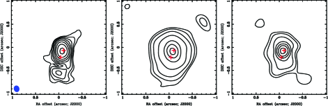
Figure 3.— This three panel image shows the VLA 43 GHz image in the left panel. The middle and right panel are CARMA 111.1 GHz A + B array image and a 222.2 GHz B-array image convolved to the same beam size as the VLA image (0$\farcs$14 $\times$ 0$\farcs$12 at P.A. 14.5^∘). The beam is plotted in the lower left corner of the VLA image. The red $+$ signs mark the positions of the Beuther et al. (2017) continuum sources cm1 and cm2. The position of source cm1 agrees within errors with what we identify as IRS 1. In all these images the reference position (0^′′,0^′′) is at RA (J2000) = 23^h13^m45${}^{s}.$383, Dec (J2000) = $+$61^∘ 28^′10$\farcs$506.

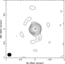
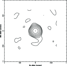
Figure 4.— High spatial resolution CARMA A array wide band images at 227.4 GHz, both formed by shift and add and reduced independently, see Section 2.2 Both images look essentially identical. Left: The December 7 continuum image, which used H30$\alpha$ for selfcal. The synthesized beam is 0$\farcs$15 $\times$ 0$\farcs$13 P.A. = 89^∘. Here we also marked the positions of the Beuther et al. (2017) continuum sources cm1 and cm2. Right: The December 6 continuum image, which used a 500 MHz wide continuum channel for selfcal. The synthesized beam size is 0$\farcs$16 $\times$ 0$\farcs$13 P.A. = 86^∘.

Table 3Gaussian fits to the IRS 1 core.

227.4 & A 0600 - 1400 k$\lambda$ 0$\farcs$16 $\times$ 0$\farcs$13 P.A. = $+$86^∘ 0$\farcs$101 $\pm$ 0$\farcs$003 $\times$ 0$\farcs$080 $\pm$ 0$\farcs$003 P.A. = 0$+$5^∘$\pm$ 06^∘
227.4 A 0600 - 1400 k$\lambda$ 0$\farcs$15 $\times$ 0$\farcs$13 P.A. = $+$89^∘ 0$\farcs$099 $\pm$ 0$\farcs$004 $\times$ 0$\farcs$090 $\pm$ 0$\farcs$004 P.A. = 0$-$6^∘$\pm$ 13^∘
227.4 A 800 - 1400 k$\lambda$ 0$\farcs$1 $\times$  0$\farcs$1  P.A. = -00^∘ 0$\farcs$043 $\pm$ 0$\farcs$007 $\times$ 0$\farcs$026 $\pm$ 0$\farcs$007 P.A. = $-$15^∘$\pm$ 15^∘
222.2 B full 0$\farcs$29 $\times$ 0$\farcs$23 P.A. = $-$85^∘ 0$\farcs$140 $\pm$ 0$\farcs$010 $\times$ 0$\farcs$090 $\pm$ 0$\farcs$010 P.A. = $+$6.1^∘$\pm$ 8^∘
111.1 A full 0$\farcs$32 $\times$ 0$\farcs$28 P.A. = $-$83^∘ 0$\farcs$150 $\pm$ 0$\farcs$010 $\times$ 0$\farcs$050 $\pm$ 0$\farcs$010 P.A. = $+$0.9^∘$\pm$ 5^∘

Fig. 3 shows the 43 GHz image from (Sandell et al., 2009) together with a high resolution CARMA A + B array images at 111.1 GHz and a CARMA B-array image at 222.2 GHz. All three images show a compact core centered on IRS 1 surrounded by faint extended emission to the south, i.e., what Gaume et al. (1995) called “south spherical”. At 111.1 GHz the morphology of the emission looks very similar to the 43 GHz VLA image, suggesting that all the emission is free-free emission. At 222.2 GHz there is a hint of a more east-west structure as well as a more pronounced tail to the southwest. It is therefore likely that we start to pick up some dust emission in the interface region between the free-free outflow and the surrounding dense infalling envelope. It is unclear whether any of this dust emission is due to the accretion disk, which should be aligned east-west, i.e., orthogonal to the outflow. This faint emission is more extended in the E-W direction and there is no sign of the northwestern extension. In the south the emission is less extended and curves more to the southwest. At the highest angular resolution, i.e. the CARMA A-array images at 227.4 GHz, the faint extended emission is filtered out, and we only see a compact core with a tail towards the southwest, see Fig. 4.

To determine the size of the compact structure seen at 227.4 GHz, we created images with three different weightings, robust = -2, 0.5 and 2, with the full uv-range (40 – 1400 k$\lambda$), as well as restricting the short spacings to 500, 600, and 800 k$\lambda$. The size of the IRS 1 core shrinks in size with improved spatial resolution, although the position angle stays the same, i.e. roughly north south. The core is barely resolved for the uv-range 800 – 1400 k$\lambda$, where the beam size is $\sim$ 0$\farcs$1, see Table 3. At this resolution the flux density of the compact core is 1.18 $\pm$ 0.05 Jy, or about a third of the total flux density (Zhu et al., 2013; Frau et al., 2014). Table 3 also gives the source sizes for 111 GHz and the 222 GHz B-array image. For these we determined the deconvolved source size by fitting a double Gaussian, one for the extended free-free jet and one for the compact core.

We also made images of the H30$\alpha$ emission with $\sim$1 and $\sim$10 km s^-1 spectral resolution. The H30$\alpha$ emission (line minus continuum) is more compact than the continuum emission with a deconvolved size 72$\times$67 mas extended in a PA $-$50 $\pm$ 10 ^∘. Fig. 5 shows moment 0 and moment 1 images made from spectral channels above a 3-sigma threshold. A velocity gradient in a NE direction (PA $\sim$ 30 $\pm$ 10) is seen in the moment 1 image at both 1 and 10 km s^-1 resolution. The gradient was confirmed by Gaussian fits to the velocity channels. In order to check if the observed velocity gradient might be due to some instrumental effect, we made a spectral image for the same wide band spectral window in the December 6 2011 observations. No spectral gradient was seen in these data; Gaussian fits to the spectral channels in the 500 MHz spectral window agrees in position within 0$\farcs$001. The velocity gradient of the H30$\alpha$ emission agrees quite well in PA with the velocity gradient that Zhu et al. (2013) found, 43^∘, in subarcsecond imaging of OCS(19–18), CH₃CN(12–11) and ¹³CO(2–1).

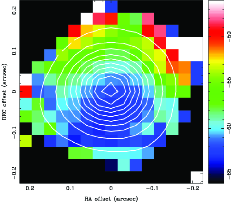
Figure 5.— Moment 0 and moment 1 images of the the H30$\alpha$ emission made from spectral channels above a 3-sigma threshold. The moment 0 emission is plotted with contours on top of the moment 1 map in color. The velocity scale is shown in the bar to the right. The images were made with a spectral resolution of 10 km s^-1. A velocity gradient in a NE direction (PA $\sim$ 30^∘ $\pm$ 10^∘) is seen in the moment 1 image.

Figure 6.— The H30$\alpha$ spectrum fitted with a three component Gaussian. The red and the blue-shifted spectral components are separated by 0$\farcs$005 in RA and 0$\farcs$009 in DEC.

The distribution of the integrated line emission is orthogonal to the velocity gradient. The structure of the H30$\alpha$ emission is unclear, because it is not aligned with the large scale ionized jet. The elongation and velocity gradient could arise from a prolate rotating structure, or be due to infall onto or outflow from an inclined disk. The fitted major and minor axis are consistent with an inclination 21 degrees (zero = face-on), although this is not consistent with the outflow, which suggests that the outflow is almost in the plane of the sky. Further evidence for an asymmetric H30$\alpha$ distribution comes from the H30$\alpha$ spectrum shown in Fig. 6, where a three component Gaussian fit is shown. Images of the red- and the blue-shifted spectral components are separated by 0$\farcs$005 in RA and 0$\farcs$009 in DEC. Gaussian fits show the red-shifted emission (-50 to 0 km s^-1) is offset to the NE in PA 30 degrees from the blue-shifted emission (-110 to -60 km s^-1). The red-shifted component is also somewhat larger (81 x 74 mas), than the blue-shifted component (60 x 54 mas). The dip in the spectrum at $\sim$ -56 km s^-1 might be produced by a colder envelope. Even at larger angular scales the hydrogen recombination line emission appears rather chaotic. Gaume et al. (1995) imaged H66$\alpha$ with the VLA at 300 AU resolution. They found extremely wide lines, 250km s^-1 toward the IRS 1 core, but no clear velocity gradient along the ionized jet. With the upgraded Karl Jansky VLA it would now be possible to image recombination lines of the ionized jet further out, where the ionized gas would not be affected by accretion and where the velocity field might be more well ordered.

There is no sign of the three linear maser features that Goddi, Zhang & Moscadelli (2015) argued to be individual H II regions. Therefore, these are more likely to be associated with the outflow (De Buizer, 2003) or photoionized pre-existent clumps of molecular material (De Buizer & Minier, 2005) rather than self luminous objects. The 227.4 GHz observations with an angular resolution of 0${}^{\prime\prime}\mskip-7.6mu.\,$1 show only a single compact, barely resolved source, and there is no evidence for IRS 1 being a binary with components cm1 and cm2 as suggested by Beuther et al. (2017). The position of the compact core is consistent with source cm1 within positional errors and also with the single compact source detected at 219 GHz (resolution 0$\farcs$33 $\times$ 0$\farcs$32) using NOEMA by Beuther et al. (2017). IRS 1 could still be a binary, but if it is, the separation between the two stars must be less than 30 AU if the binary components have roughly equal brightness.

IRS 1 has a total luminosity of 1.1 – 1.4 10⁵  L_⊙ (corrected to a distance of 2.65 kpc), as determined from extinction corrected near/mid IR observations (Willner, 1976; Hackwell, Grasdalen & Gehrz, 1982) and modeling of the observed dust emission surrounding IRS 1 (Akabane & Kuno, 2005). We have independently checked the bolometric luminosity of IRS 1 by integrating over the observed SED, which includes accurate high angular resolution far-infrared SPIRE, PACS, and FORCAST images from 500 $\mu$m – 19 $\mu$m. Using published photometry from 2.2 $\mu$ to 1.3 mm, including the photometry derived in this paper (Table 1 & 2), we get a bolometric luminosity of 1.0 10⁵  L_⊙. Here we used the PACS and SPIRE integrated flux densities in Table 2 to include heating from IRS 1 into the surrounding core, although it does not really make much of a difference, because the bulk of the luminosity comes from shorter wavelengths. This is a lower limit to the total bolometric luminosity, because we know that a significant amount of FUV light escapes into the outflow without heating up the cloud envelope surrounding IRS 1.

The observed luminosity corresponds to an O7 star, if the central source is a single star. The spectral type determined from free-free emission has resulted in somewhat later spectral types, O8 - B0 ZAMS (see e.g., Hackwell, Grasdalen & Gehrz, 1982; Akabane & Kuno, 2005; Zhu et al., 2013), because the ionizing flux has been estimated at a wavelength where the free-free emission is still significantly optically thick. Shi Hui (2015, personal communication) derives a spectral type of $\sim$ O5.5 from modeling high spatial resolution VLA and mm-interferometry data, which is more consistent with the observed bolometric luminosity.

We have refined the mass estimate for the IRS1 envelope using the published single dish data complemented with the FORCAST & Herschel data in Tables 1 & 2. Here we used a two-component graybody fit to the observed flux densities from 1.3 mm to 20 $\mu$m, thereby avoiding contribution from the hot dust which dominates the emission at near-IR wavelength. For the cold extended envelope surrounding IRS 1 our fit predicts a size of $\sim$ 20^′′, a dust temperature of $\sim$ 40 K, and a dust emissivity index, $\beta$ = 1.80, resulting in a total mass (gas + dust) of 490  M_⊙. The fit predicts a size of 5$\farcs$7 and a temperature of 81 K for the warm inner envelope surrounding IRS 1. The dust emissivity index for the warm component was fixed at $\beta$ = 1.5. We performed a similar fit for the extended 50^′′ – 60^′′ cloud core surrounding the IRS 1 – 3 cluster and obtained similar temperatures and sizes for the warm dust component. The temperature is about the same for the cold cloud core, $\sim$ 42 K, while the dust emissivity index is slightly lower, $\beta$ = 1.6, resulting in a total mass of 1,300  M_⊙.

4. The IRS 1 molecular outflow

Figure 7.— a) 8 $\mu$m IRAC image plotted with a logarithmic stretch. IRS 1 at 0^′′,0^′′ is at RA (J2000) = 23^h13^m45^s.383, Dec (J2000) = $+$61^∘ 28^′10$\farcs$506. To the NW we see the large cavity created by the NGC 7538 H II region, which is surrounded by PAH emission except on the western side. There is a second cavity extending up to 250^′′ from IRS 1, which has been cleared out of the surrounding cloud by the outflow from IRS 1. To the southwest one can see a faint fan-shaped plume of emission, which emerges out of the cloud and ends in a bow-shock like emission feature. This is almost certainly the counter-flow to the large northern blue-shifted outflow. IRS 9 is outside of the image to the east, but one can see some emission from it at $\sim$ 100^′′,-50^′′. The second bright (yellow) source is IRS 4. IRS 1, IRS 4, IRS 11 and (NGC 7538) South are labeled. b) The same image overlaid with high velocity CO(3–2) in contours. The blue-shifted emission is averaged from -82 – -64 km s^-1 and plotted with eight linearly spaced blue contours going from 0.3 – 3.8 K, while the red-shifted emission is averaged from -52 – -31 km s^-1 and plotted with eight contours from 0.8 – 6.5 K. Some of the emission seen in the red-shifted emission is due to a large extended cloud south and southwest of IRS 1 at -50 km s^-1, which overlaps with the NGC 7538 molecular cloud at $\sim$ -58 km s^-1 (see Fig. A.1). The solid black line is drawn through IRS 1 at a PA of 10^∘ and shows the approximate symmetry axis for the whole blue-shifted outflow lobe. Close to IRS 1 the PA is $\sim$ 0^∘ both for the high velocity molecular gas and the ionized jet.

4.1. Background

It has been widely accepted that IRS 1 drives a bipolar molecular outflow at a P.A. of $\sim$ 145^∘ (Scoville et al., 1986; Kameya et al., 1989; Davis et al., 1998; Qiu, Zhang & Menten, 2011), although other outflows from the young cluster surrounding IRS 1 may also contribute (Qiu, Zhang & Menten, 2011). Kraus et al. (2006) suggested that the outflow from IRS 1 is precessing and has therefore created a wide-angled outflow. However, it is hard to think of a mechanism, where the ionized outflow and the molecular outflow would be completely misaligned. Molecular outflows are secondary phenomena, which are shaped by their interaction between the wind and the surrounding cloud. It is therefore possible that the high velocity gas close to IRS 1 may give a distorted view of the molecular outflow, especially because of the extreme accretion rate towards IRS 1. Sandell et al. (2012) noticed a large fan shaped outflow protruding out of the molecular cloud south of IRS 1 on Spitzer IRAC images of NGC 7538. This fan shaped nebula points back towards IRS 1. In the north there is a large, elongated cavity, also pointing back towards IRS 1. The northernmost part of this cavity could not have been excavated by the NGC 7538 H II region, because all the O stars illuminating it are too far west of it as seen in projection, so the real separation could be even larger. The only star luminous enough to create such a cavity is IRS 1. In the 8 $\mu$m IRAC color image (Fig. 7) one can see the cavity extending up to $\sim$ 250^′′, i.e., 3.2 pc, from IRS 1. In the south a fan shape nebulosity emerges out of the cloud and curving to the west. The tip of the nebulosity is quite bright and almost certainly a bowshock, since there is no infrared source embedded in it. This bow shock, seen at -100^′′, -180^′′ in Fig 7 is $\sim$ 200^′′ (2.6 pc) south of IRS 1

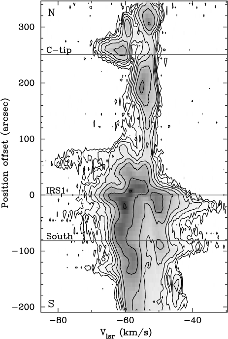
Figure 8.— Position-velocity (pv) diagram in gray scale overlaid with contours of CO(3–2). The pv cut goes through IRS 1 along the symmetry axis (PA = 10^∘) of the IRS 1 outflow as shown in Fig. 7 b. IRS 1 is at offset 0^′′. The tip of the blue-shifted outflow is $\sim$ 280^′′ (3.6 pc) from IRS 1. South of IRS 1 one can see both blue- and red-shifted emission, some of which maybe due to embedded young stars in the dense molecular cloud. The cut goes west of NGC 7538 South and misses the blue outflow lobe from the star, but picks up red-shifted emission to the south of the star. We have marked and labelled the tip of the northern cavity (C-tip) seen at 8 $\mu$m (Fig. 7), the location of IRS 1, and NGC 7538 South with gray horizontal lines. The contours are logarithmic with eight contours going from 0.5 – 22 K.

4.2. The large N-S outflow as seen in CO(3–2)

In Fig. 7b we have plotted blue- and red-shifted CO(3–2) overlaid in contours on the same 8 $\mu$m image seen in Fig. 7 a. The strongest high velocity emission is close to IRS 1 with the red (SE) and the blue-shifted (NW) emission peaks separated by $\sim$ 30^′′ at a PA of 125^∘ - 135^∘, which agrees with earlier studies. However, there is still strong blue-shifted emission extending up to $\sim$ 80^′′ north of IRS 1, i.e., approximately where the large cavity becomes apparent in the 8 $\mu$m image. At the northern end of this cavity blue-shifted emission again becomes visible, where the outflow interacts with the surrounding molecular cloud. The extent of the southern outflow is less clear in CO(3–2). South of IRS 1 there is both blue- and red-shifted emission, suggesting that the dense molecular cloud has affected the outflow, making it largely flow in the plane of the sky, i.e., perpendicular to us. We also see the “compact” outflow from NGC 7538 South, which is located $\sim$ 80^′′ south of IRS 1 and within the expected path of the southern outflow. A further complication in the south is the rather strong emission from the -50 km s^-1 cloud, see Fig A.1, which also appears to be connected to the NGC 7538 H II region. The strong NW-SE outflow seen at low to moderate velocities in low J CO lines is somewhat puzzling. As we will see later on, this high velocity emission is not seen in high CO or in [C ii]. The most likely explanation is that most of this outflow emission is from young embedded low to intermediate protostars in the IRS 1 core. Especially the northwestern blue-shifted emission lobe appears to point toward the protostar MM 4, as shown in the high resolution SMA CO(2–1) image by Qiu, Zhang & Menten (2011).

Figure 9.— High velocity [C ii] emission in blue- and red contours overlaid on a smaller IRAC 8 $\mu$m image than in Fig. 7 and plotted with a logarithmic stretch. IRS 1 is at 0^′′, 0^′′ and marked with a red star symbol. The blue-shifted emission is averaged from -74 km s^-1 - -64 km s^-1. and plotted with 8 linear contours going from 0.75 K to 3.5 K. The red-shifted emission is averaged from -52 km s^-1 - -42 km s^-1and plotted with 8 linear contours from 0.75 K to 2.5 K. The red-shifted peak at $\sim$ 52^′′, -32^′′} is a bright peak in the -50 km s^-1 cloud and not associated with any outflow. The red-shifted emission NE of IRS 1 at PA $\sim$ 45^∘ is true high velocity emission. IRS 1, IRS 4, IRS 11 and (NGC 7538) South are labeled.

The position-velocity plot of CO(3–2) (Fig. 8) shows the northern blue-shifted high velocity gas quite well. The CO emission is very broad at the leading edge of the high velocity cloudlets at 60^′′ – 80^′′ north of IRS 1, where the outflow becomes invisible, because there is no molecular gas to interact with. The outflow becomes visible again where it plunges into the surrounding cloud again at $\sim$ 240^′′ north of IRS 1. Here the outflow velocity is more modest, $\sim$ 10 km s^-1, most likely because there is still considerable mass in the surrounding cloud. To the south the outflow appears both blue and red-shifted. Although the position-velocity plot picks up the outflow from NGC 7538 South, this outflow cannot explain the high velocity emission seen to the south, because the outflow from South is very compact (Sandell & Wright, 2010). It is therefore likely that most of this high velocity emission is driven by IRS 1. There is a “bowshock” seen in blue-shifted emission $\sim$ 140^′′ south of IRS 1 where the outflow emerges out of large NGC 7538 cloud core, i.e., the dense, massive core at $\sim$ -58 km s^-1.

4.3. The IRS 1 outflow in [C ii] 158 $\mu$m emission

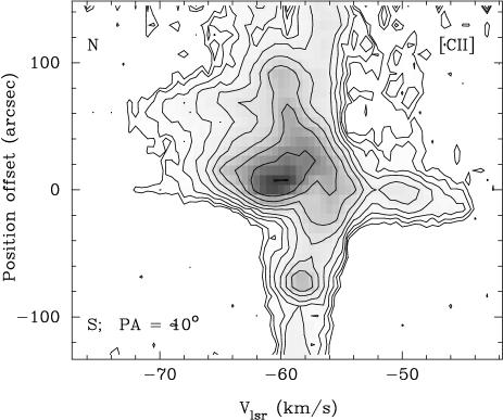
Figure 10.— Position-velocity diagram in gray scale overlaid with contours of [C ii] through IRS 1 at a P.A. = 10^∘, i.e. at the same PA as CO(3–2) in Fig. 8. IRS 1 is at offset 0^′′. The velocity structure of the [C ii] emission looks almost identical to that of CO(3–2), except close to IRS 1 where one sees strong emission from the compact H II region IRS 2, which is 8^′′north of IRS 1. The contours are logarithmic with eight contours going from 0.5 – 22 K.

The [C ii] fine structure line is not an outflow tracer. It is a PDR tracer (Tielens & Hollenbach, 1985; Hollenbach & Tielens, 1999). Although some [C ii] emission can be produced in shocks (Flower & Pineau des Forêts, 2010), it is two to several orders of magnitude fainter than the PDR emission. Yet [C ii] emission is seen toward many outflows (van Kempen et al., 2010; Podio et al., 2012; Alonso-Martínes et al., 2017). In most cases the [C ii] originates from PDR emission in the surrounding cloud, but there are also some cases where one might see [C ii] emission from the cavity walls of the outflow or from UV irradiated shocks in the outflow(Visser et al., 2012; Green et al., 2013; Alonso-Martínes et al., 2017). Fig. 9 shows that the blue-shifted high velocity [C ii] emission fills the outflow lobe and looks similar to the blue-shifted CO(3–2) at high velocities. We definitely see [C ii] emission from IRS 2, because it is a bright compact H II region and the peak of the [C ii] emission is approximately centered on IRS 2. IRS 2, however, does not have an outflow. Observations of the [Ne ii] fine structure line at 12.8 $\mu$m, shows that it has ionized gas in the velocity range -82 km s^-1– -51 km s^-1 (Zhu et al., 2008). There is no sign of low-velocity [C II] tracing the cavity walls of the outflow. It appears that the strong FUV radiation from IRS 1 ionizes some of carbon in the fast moving CO cloudlets resulting in strong PDR emission tracing the surface layers of the cloudlets. The emission knot at 53^′′, -32^′′ seen in red-shifted [C ii] (Fig. 9) is not an outflow. The [C ii] channel maps (Fig. A.2) show that it is only seen in the channels centered at -51 and -47.5 km s^-1. It is unclear what star illuminates this PDR. There is not much high velocity red-shifted [C ii] emission south of IRS 1, although we see strong [C ii] emission in the velocity range from $\sim$ -60 to -50 km s^-1 south and north-west of IRS 1 (see the channel maps in Fig. A.2). Most of this emission is likely to be PDR emission illuminated by the NGC 7538 H II. There is no [C ii] emission associated with the compact NGC 7538 South outflow, which is very prominent in CO(11–10), see Section 4.4. However, in the the channel maps we see a compact, $\sim$ 10^′′ knot of emission in the channel centered on -58 km s^-1 about 70^′′ south of IRS 1 (Fig. A.2). The position of this knot is within 1^′′ of IRS 11, a well known young Herbig Be star near NGC 7538 South. The deeply embedded IRS 11 apparently illuminates a small nebula, which we see in [C ii]. This PDR emission is also seen in the [C ii] position velocity diagram at $\sim$ 70^′′ south of IRS 1 (Fig. 10).

The blue-shifted emission north of IRS 1 has the same velocity structure as CO(3–2) (Fig. 10) with the leading bowshock at 80^′′ north of IRS1 having the highest velocities. The highest velocity seen in [C ii] is -74 km s^-1 whereas it is $\sim$ -85 km s^-1 in CO(3–2). The difference is most likely due to the lower sensitivity (shorter integration times) in [C ii]. Using observations with longer integration times we find that the high velocity emission has very much the same extent in both [C ii] and CO(3–2), toward IRS,1 (Fig. 11). Both [C ii] and CO(3–2) show high velocity wings of $\pm$ 40 km s^-1 or more.

There are also some clear differences between [C ii] and CO(3–2). The dominant red-shifted (SE) and blue-shifted (NW) outflow lobes near IRS 1 are far less obvious in [C ii] than in CO(3–2), see Fig. 8 & 10.

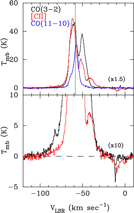
Figure 11.— Long integration [C ii] (red), CO(11–10) (blue), and CO(3–2) (black) spectra in native angular resolution toward NGC 7538 IRS 1. The gray vertical line in the top panel marks the systemic velocity, -58.5 km s^-1. In the top panel the CO(3-2) brightness temperature is multiplied by a factor of 1.5, in the bottom one, which shows the high velocity wings it is scaled by a factor of 10. The faint absorption between -12 - 0 km s^-1 is due to emission or absorption from gas in the local arm. In [C ii] it is absorption against the strong continuum from IRS 1. In CO(3–2) it is due to emission in the reference position.

4.4. CO(11–10)

Figure 12.— High velocity CO(11-10) emission in blue- and red contours overlaid on an IRAC 8 $\mu$m image plotted with a logarithmic stretch. IRS 1 is at 0^′′, 0^′′. The blue-shifted emission is averaged from -66 km s^-1 - -60.5 km s^-1. and plotted with 8 logarithmic contours going from 0.45 K to 4.8 K. The red-shifted emission is averaged from -56 km s^-1 - -50.5 km s^-1 and plotted with 6 linear contours from 0.5 K to 2.7 K. IRS 1, IRS 4, IRS 11 and (NGC 7538) South are labeled.

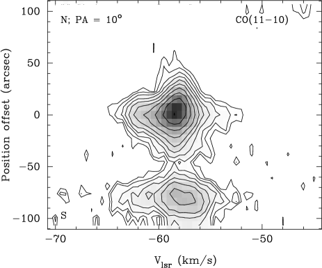
Figure 13.— Position-velocity diagram in gray scale overlaid with contours of CO(11–10) through IRS 1 at PA = 10^∘, i.e. the same as for CO(3–2) and [C ii]. IRS 1 is at offset 0^′′. The compact outflow from the young high mass star NGC 7538 South at $\sim$ 81^′′ to the south is quite prominent in blue-shifted emission. CO(11–10) emission still continues to the south. The contours are logarithmic with ten contours going from 0.8 – 29 K.

CO(11–10) was observed simultaneously with [C ii] in the L1 channel of GREAT. Since L1 is a single pixel receiver, the CO(11–10) map is not as extended as the [C ii] map. One would expect that the emission from CO(11–10), which has a critical density of 4 $\times$ 10⁵ cm^-3 for a gas temperature of 100 K (Yang et al., 2010), would be quite compact. Yet CO(11–10) emission extends almost all the way to NGC 7538 South, 80^′′ south of IRS 1 (Fig. 12). South of IRS 1 the outflow velocities are rather modest, with line wings $\sim$ 3 km s^-1 in both blue- and red-shifted gas to $\sim$ 40^′′ south of IRS 1 (Fig. 12 & 13). Further south the line is very narrow until the emission runs into the outflow from NGC 7538 South, where one sees strong blue- and red-shifted emission. The southern outflow lobe appears to behave very much the same way in CO(11–10) as it does in CO(3–2) and [C ii]. The outflow is at near-cloud velocities or perhaps even slightly blue-shifted, suggesting that the southern outflow lobe is close to the plane of the sky. The emission in CO(11–10) is undoubtedly excited by the outflow, because CO(11–10) is only seen along the expected path of the outflow. Only hot gas in the outflow can excite CO to such high energy levels. The velocity of the northern outflow is low and only seen to $\sim$ 40^′′ north of IRS 1. The high-velocity cloudlets, which stand out prominently in CO(3–2) and [C ii], are too diffuse to excite CO(11–10). There is no sign of the SE-NW outflow lobes, which dominate the outflow near IRS 1 in low J CO lines and other low excitation tracers, like HCO⁺.

4.5. The morphology of the outflow near IRS 1; CARMA CO(1-0) and ¹³CO(1-0) imaging

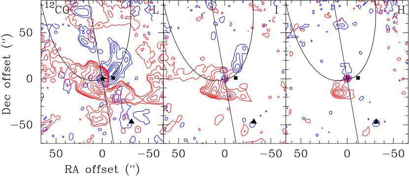
Figure 14.— Contour plots of the low, intermediate and high velocity blue- and red-shifted CO(1–0) emission from CARMA observations with 4${}^{\prime\prime}\mskip-7.6mu.\,$5 spatial resolution. Due to the primary beam correction the maps are noisier in the northernmost part of the map, because it is close the HPBW of the CARMA primary beam. The L panel shows low velocity emission, $\pm$9 km s^-1 from the systemic velocity, -58.5 km s^-1, averaged over a 6.4 km s^-1 wide velocity interval. The I panel shows the outflow at intermediate velocities, $\pm$15 km s^-1, also averaged over a 6.4 km s^-1 wide velocity interval, while the H panel shows high velocity emission, $\pm$25 km s^-1 from the systemic velocity averaged over a 14 km s^-1 wide window. At low and intermediate velocities we see blue-shifted emission from the cloudlets in the blue-shifted outflow lobes. At higher velocities the outflow is more jet-like and aligned with the ionized jet. The contour levels for the low and intermediate velocities are at 0.9, 3, 7, 12, 18, and 25 K, and at 0.5, 1.5, 3, 4.5, and 7 K for the high velocity panel (right). IRS 1 is at 0^′′, 0^′′ and marked with a star symbol on the L panel. Also marked with a black square symbol is the sub-millimeter and H₂O maser source MM 4 (Qiu, Zhang & Menten, 2011), which almost certainly contributes to the blue-shifted high velocity emission NW of IRS 1. We also marked another H₂O maser with a black triangle at offset -31^′′,-47^′′. This source appears to be associated with a compact blue-shifted high velocity knot. We also drawn the symmetry axis of the outflow and our best guess of the boundary between the outflow cavity and the surrounding cloud. These are plotted in black on each panel.

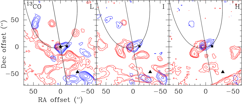
Figure 15.— Contour plots of the low, intermediate and high velocity blue- and red-shifted ¹³CO(1–0) emission from CARMA observations imaged with a beam size of 7${}^{\prime\prime}\mskip-7.6mu.\,$9 $\times$7${}^{\prime\prime}\mskip-7.6mu.\,$4 p.a. = 55 ^∘ resolution and zero spacings from OSO 20 m observations plotted the same way as in Fig. 14. In the L panel the blue-shifted emission is centered at -61.3 km s^-1 and the red-shifted emission at -52 km s^-1, both averaged over a 1.66 km s^-1 wide window. In the I panel the center velocities for the blue- and red-shifted emission is -63 km s^-1 and -50.2 km s^-1with 1.66 km s^-1and 2.0 km s^-1 wide windows for blue- and red-shifted emission respectively. In the H panel the blue- and red-shifted center velocities are -64.8 km s^-1 and -47.5 km s^-1, averaged over 2 and 3.3 km s^-1, respectively. The contour levels for the low velocities are at 0.9, 1.4, 2, 3, 4.5, and 6 K, for intermediate velocities at 0.5, 0.9, 1.7, 3.5, and 5 K and for the high velocities (right panel) at 0.3, 0.5, 0.8, 1.4, and 2.5 K. All the rest is plotted as in Fig. 14.

Single dish images do not have enough spatial resolution to show how the outflow behaves near IRS 1. We therefore also make use of some CARMA images of CO(1–0) and ¹³CO(1–0), the latter filled in for missing zero spacing with maps from the OSO 20 m telescope, see Sect. 2.3. The emission from the surrounding molecular cloud is very strong and it is difficult to study the outflow at low velocities, especially in ¹²CO. In Fig. 14 the lowest blue- and red-shifted emission starts at $\sim$6 km s^-1 from the systemic velocity of the cloud. Some of the red-shifted emission, however, is not from the IRS 1 outflow, but from gas associated with the expanding H II NGC 7538 NW of IRS 1, see e.g. Davis et al. (1998), or from dense condensations in the “-50 km s^-1” cloud. The ¹³CO, which is more optically thin, can probe the outflow at lower velocities but it is difficult to evaluate, especially for red-shifted velocities, because of contamination from the extended “-50 km s^-1” cloud. This cloud has several velocity components between -52 and -45 km s^-1, some of which also appear to trace the PDR layer associated with NGC 7538. The cluster of sub-millimeter sources (Qiu, Zhang & Menten, 2011) most likely power molecular outflows as well. Some of the blue-shifted emission NW of IRS 1 is likely from MM 4, which is shown as a filled black square in Figs. 14 & 15. Some of the red-shifted emission south of IRS 1 is almost certainly “contaminated” by emission from one or several of these sub-millimeter sources as well.

At low velocities the ¹³CO emission is red-shifted East and EW of IRS 1. There is also some red-shifted emission to the NW, Fig.15. One can also see some red-shifted emission associated with the high velocity cloudlets near the symmetry axis of the blue-shifted outflow. ¹²CO(1–0) behaves the same way as ¹³CO at low and intermediate velocities, i.e. it strongly suggests that the outflow is rotating, possibly in a spiral pattern (Wright et al., 2014). What is noticeable is that at high spatial resolution the high velocity jet or high velocity cloudlets inside the blue-shifted outflow lobe break up into compact clumps. At intermediate velocities the clumps become more centered in the middle of the outflow lobe, see panel I in Fig. 14. At high velocities the blue-shifted outflow is well collimated, almost N-S, like the free-free jet, and extending to $\sim$15^′′ N of IRS 1. At these velocities we no longer see the northwestern blue-shifted outflow feature, which dominates at lower velocities.

4.6. What we learned about the outflow from CO(3–2), [C ii] and CO(11–10)

Here we summarize what we learned about the morphology of the large scale IRS 1 outflow from examination of CO(3–2), [C ii] and CO(11–10). The large CO(3–2) map confirms that the large cavity north of IRS 1 seen in IRAC images has been created by the molecular outflow from IRS 1. We can trace the outflow in high velocity blue-shifted emission up to about 80^′′ north IRS 1 after which it becomes invisible due to the low gas density of the surrounding cloud. At the tip of the outflow, $\sim$ 250^′′ to the north, the outflow again becomes visible as blue-shifted CO(3–2) high velocity emission where it hits the dense surrounding molecular cloud. The southern outflow from IRS 1 is probably deflected by the dense molecular cloud south of IRS 1 and is almost in the plane of the sky. Therefore it is seen as mostly blue- and red-shifted low velocity emission. The southern outflow passes close to NGC 7538 South, another young high mass star and becomes invisible when the density of the surrounding cloud becomes to low to excite CO emission. The plume seen in IRAC images where the outflow emerges out of the cloud appears to contain no or very little molecular gas.

These findings are strongly supported by the smaller maps we have obtained in [C ii] and CO(11–10). The high velocity clouds or cloudlets in the northern outflow lobe are also seen in [C ii], where they show the same morphology and velocity structure as seen in the CO(3–2) high velocity emission. This suggest that they are illuminated by the strong UV radiation escaping from IRS 1 into the outflow. They are not seen in CO(11–10), most likely because they have too low gas density to excite CO(11–10). The outflow from IRS 1 also has modest blue- and red-shifted velocities south of IRS 1 in [C ii] and CO(11–10) confirming that the southern outflow lobe is almost in the plane of the sky. However, since we trace CO(11–10) emission almost all the way to NGC 7538 South, this emission must be excited by IRS 1, since CO(11–10) has a critical density of 4 $\times$ 10⁵ cm^-3 and an upper energy level of 304.2 K. No other mechanism can produce such warm high density gas in this region, except radiation from IRS 1.

4.7. Outflow properties

We use the CO(3–2) map to to estimate the physical properties of the outflow, because it is the only outflow tracer we have, which covers the whole outflow. We restrict the analysis to the blue-shifted outflow lobe, because it is clearly defined with very little contamination for the surrounding cloud. It is harder to extract information from the counter-flow (”red”-shifted), because of the strong cloud emission and contamination from other outflows. It is not possible to directly estimate the inclination of the blue-shifted outflow lobe, but it appears to be close to the plane of the sky. Here we assume an inclination of 70^∘ $\pm$ 10^∘. If we use the total extent of the blue-shifted outflow, 3.6 pc, a velocity of 10 km s^-1 ( see Fig 8), we get t_dyn $\sim$ 1.3 $\times$ 10⁵ yr after correcting for inclination. This estimate has an uncertainty of about a factor of two due to the uncertainty in the inclination. Usually dynamical timescales are under-estimates, see e.g. Parker, Padman & Scott (1991). When an outflow first starts, it has to drill through dense gas, so it starts slowly. Then once the density gets lower (and it does seek the path of least resistance), the outflow speeds up. How long this phase takes is hard to estimate. After that it may move with relatively constant velocity as long as the gas density is relatively uniform, which is definitely not the case here. Nevertheless, here we will use the dynamical time scale derived above, i.e. 1.3 $\times$ 10⁵ yr. For estimating physical parameters of the outflow, like mass, momentum and kinetic energy, we use the large JCMT CO(3–2) map, which is the only data set we have that covers the whole outflow. Here we only analyze the northern blue-shifted outflow lobe, because it is well defined and only moderately affected by the surrounding molecular cloud, where as the same is not true for the southern outflow, which is strongly affected by the dense molecular cloud south of IRS 1. There may be some contribution from outflows from embedded lower mass protostars (Qiu, Zhang & Menten, 2011), but the IRS 1 outflow will dominate overall. CO(3–2), however, is extremely optically thick, and we do not have ¹³CO(3–2) maps covering more than a small portion of the outflow. To get an idea of the ¹²CO optical depth we therefore use the deep HARP CO(3–2) and ¹³CO(3–2) maps, which are centered on IRS 1 and cover $\sim$ 100^′′ $\times$ 100^′′ and 80^′′  $\times$ 80^′′ for ¹²CO(3–2) and ¹³CO(3–2) respectively. These maps show that ¹²CO is significantly optically thick over all outflow velocities seen in ¹³CO, or up to blue-shifted velocities of $>$ 20 km s^-1 from the systemic velocity, here assumed to be -58.5 km s^-1. This is shown in Fig.16, where we show the ¹²CO(3–2) and ¹³CO(3–2) spectra in the top panel and the ratio of ¹²CO(3–2) to ¹³CO(3–2) in the bottom panel. This figure shows that ¹²CO is optically thick over the velocity range were we detect ¹³CO emission, Here we have assumed a ¹²C to ¹³C ratio of 79 (Wilson & Rood, 1994) and scaled the ¹³CO(3–2) by 7.9, i.e. the ratio would be 10 if ¹²CO(3–2) is optically thin. However, ¹²CO(3–2) is not only optically thick on IRS 1, similar ratios are seen over the whole area mapped in ¹³CO(3–2), indicating that ¹²CO is likely to be optically thick over a large part of the outflow.

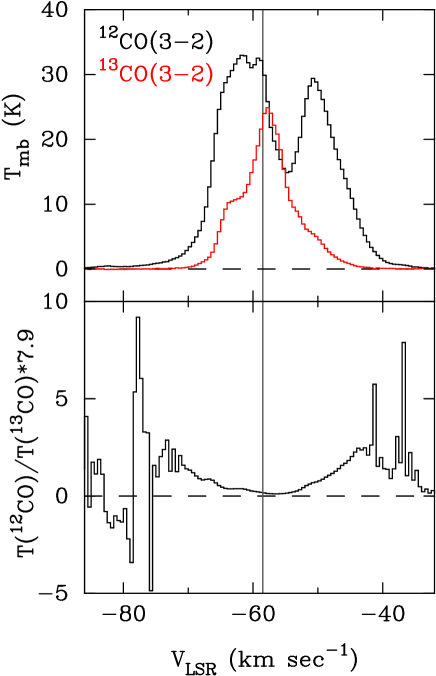
Figure 16.— The top panel shows long integration ¹²CO(3–2) and ¹³CO(3–2) spectra, the latter plotted in red, toward IRS 1. The bottom panel shows the ratio of T_mb(¹²CO) over T_mb(¹³CO), with ¹³CO multiplied by a factor of 7.9, i.e. a ratio of 10 corresponds to optically thin ¹²CO(3–2) emission. This shows that ¹²CO(3–2) is significantly optically thick over the whole velocity range, where we see the high velocity gas in ¹³CO, i.e. to $\sim$ -78 km s^-1, or $\sim$ 20 km s^-1 from the systemic velocity in the blue-shifted outflow wing. At high outflow velocities the ratio is dominated by the noise in the spectra. The gray vertical line marks the systemic velocity, -58.5 km s^-1. There are two clouds in the direction of IRS1, one at -58 km s^-1 and the other one, which is more diffuse at $\sim$ -50 km s^-1. The -58 km s^-1 cloud is self absorbed in ¹²CO. Hence the two clouds look about equal in ¹²CO, while the -50 km s^-1 cloud is fainter in ¹³CO(3–2).

To estimate the outflow parameters we therefore divided up the map into three parts. The first is a polygon encompassing the outflow around IRS 1 to 50^′′ north of the star, the second goes from there to $\sim$ 100^′′ from IRS 1 and the third one covers the tip of the outflow $\sim$ 250^′′ to the north. We integrate over velocity intervals of 2.1 km s^-1 for low velocities, then gradually increasing the velocity range to 3.8 km s^-1. The highest velocity range, 20.5 km s^-1 from the systemic velocity is integrated over 6.4 km s^-1. For the area closest to IRS1 we apply the average opacity corrections derived from the ¹²CO to ¹³CO ratio. Since we don’t know what the optical depth is further out, we take half of the correction and at the tip of the outflow we assume the CO is optically thin.

The IRS 1 molecular outflow is hot. Near IRS 1 Klaassen et al. (2009); Zhu et al. (2013) find the temperature of the molecular gas is 250 K or more from analysis of methylcyanide emission toward IRS 1. Since one sees CO(11–10) emission up to more than 40^′′ from IRS 1 and strong [C ii]  emission to more than 80^′′ from IRS 1, the gas must be hot even further away from IRS 1. It is therefore clear that strong UV radiation from IRS 1 shining into the outflow cavity and illuminating the gas in the outflow is capable of heating the gas over most of the outflow. Here we have assumed a gas temperature of 100 K for our column density estimates, which is the same temperature Klaassen et al. (2011) used in their study of outflows from high mass stars. The error resulting from the uncertainty in temperature is relatively minor. A 50 K error in temperature only changes the column density by 30 – 34%, whereas errors in the ¹²CO optical depth over the outflow is likely to result in an uncertainty of a factor of two or more in the mass of the outflow. We estimate the outflow mass for optically thin emission assuming a standard CO to H₂ abundance ratio of 10^-4 (Mangum & Shirley, 2016), a mean molecular weight $\mu_{\rm{H}_{2}}$ of 2.8 per hydrogen molecule (Kauffman et al., 2008) and apply the opacity corrections as explained earlier in this section. By summing over all the velocity intervals from -61.4 km s^-1 to -82.2 km s^-1  we get a total mass of the blue-shifted outflow lobe of 45.5  M_⊙. More than 90% of the mass is the area extending up to 50^′′ from IRS 1. To calculate momentum, P, momentum flux, F, and kinetic energy, E_k, we use the formulae presented in Choi, Evans II & Jaffe (1993), although we correct for inclination assuming an outflow inclination of 70^∘. For the blue-shifted outflow we get P = 290  M_⊙km s^-1, E_k = 1.9 $\times$ 10⁴⁰ J, and F = 0.4 $\times$ 10^-2  M_⊙ km s^-1 yr^-1. If we assume that the outflow is momentum conserved, the mass in the red-shifted outflow is likely to be similar, since the outflow velocities are about the same for both the blue- and the red-shifted outflow. The same is true for the other outflow parameters. If we compare our results to Qiu, Zhang & Menten (2011) over the same velocity interval as they used, our mass estimate, 91  M_⊙ agrees quite well with their estimate, $\sim$ 100  M_⊙. We can also estimate the mass of the outflow in [C ii] emission. To compute the [C ii] column density we use equation 26 in Goldsmith et al. (2012) assuming that the [C ii]— emission is optically thin with an excitation temperature of 100 K. If we adopt 1.2 $\times$ 10^-4 for the C⁺/H abundance ratio (Wakelam & Herbst, 2008), see also Ossenkopf et al. (2015), we get a total mass of the [C ii] outflow of 18  M_⊙, by integrating the blue-shifted [C ii] emission from -74 – -61.5 km s^-1. Here we have corrected the outflow mass for contribution from IRS 2, which we know has strong blue-shifted [C ii] emission, see Section 4.3, by placing a 20^′′ aperture centred on IRS 2. The mass of gas ionized by IRS 2 is $\sim$ 3  M_⊙.

The total mass of the blue-shifted outflow is therefore $\sim$64  M_⊙, and if we assume that the mass in the red-shifted outflow is the same, the total outflow mass could be as high as 130  M_⊙, which is still less than the mass of the core of IRS,1, which we estimated to be $\sim$ 490  M_⊙, Section 3. Compared to low-mass outflows, the IRS 1 outflow is much more massive, but the mass is similar to other high mass star outflows (Beuther et al., 2002). There are examples of high mass star outflows, where the outflow mass even exceed the core mass (Shepherd et al., 1998; Qiu et al., 2009). Earlier we estimated a dynamical time scale of 1.3 $\times$ 10⁵ yr, which would give us a mass outflow rate of 1.0 10^-3  M_⊙yr^-1, which agrees reasonably well with the observed mass accretion rate.

5. Discussion

The IRS 1 – 3 region, which borders the H II region NGC 7538, is the center of a young star cluster with more than 150 young stars and protostars (Mallick et al., 2014; Sharma et al., 2017). The IRS 1 - 3 cluster is almost certainly a case of star formation triggered by the expanding NGC 7538 H II region, although it has not been conclusively proven to be the case (Balog et al., 2004; Puga et al., 2010; Sharma et al., 2017). IRS 1 is the most massive star in the cluster and it is still heavily accreting with an accretion rate in the range 10^-3 to a few times 10^-4 M_⊙/yr (Sandell et al., 2009; Klaassen et al., 2011; Qiu, Zhang & Menten, 2011; Beuther, Linz & Henning, 2012; Zhu et al., 2013), which quenches the expansion of an H II region. It is almost certainly surrounded by an accretion disk, although there is no firm evidence of such a disk, because the emission from the ionized jet powered by IRS 1 is so strong in the millimeter and submillimeter regime, that it completely hides the much fainter accretion disk.

In this paper we have analyzed high angular resolution ($\sim$ 0${}^{\prime\prime}\mskip-7.6mu.\,$1) CARMA observations at 1.3 mm which conclusively shows that none of the previously proposed companions to IRS 1 are high mass stars. It could still be a binary, but then the secondary must be within 30 AU, if the binary components have roughly equal brightness or if the secondary has a later spectral type. In a way this is somewhat surprising since most massive stars are close binaries or multiple systems (Sana et al., 2012). A single star is, however, consistent with the observed luminosity of the star, $\geq$ 1.0 10⁵  L_⊙, for which the lower limit corresponds to the luminosity of a single O7 star. If the spectral type is as early as O5.5, the secondary would have to be a later spectral type. For a spectral type of O7 – O5.5, the stellar mass would be in the range 30 – 50  M_⊙ (Davies et al., 2011).

What makes IRS 1 so extraordinary is that it is an extremely young O-star, which has such a high accretion rate that it quenches the formation of an H II region. The FUV-radiation by the star can only escape in the polar regions, where it excites a ”jet-like” ionized outflow with velocities in excess of 250 km s^-1(Gaume et al., 1995). In this paper we have also shown that the strong FUV radiation from IRS 1 heats molecular gas inside the outflow lobes and ionizes carbon, which is why we see high velocity [C ii] 158 $\mu$m emission up to $\sim$ 100^′′  (1.3 pc) north of IRS 1 in the blue-shifted outflow lobe. Most of this gas is still molecular and seen in CO(3–2), with similar morphology and velocity structure, see Figs. 8 and 10.

We can use the jet model by Reynolds (1986) to estimate the turnover frequency and the mass loss rate of the ionized jet, i.e., his Eqs. 18 and 19. In his paper Reynolds (1986) used IRS 1 as an example to illustrate of how his model could be applied. Since we now have more accurate data and knowledge of IRS 1, we can expect more robust results. From the VLA data in Sandell et al. (2009) we estimate a collimation angle of $\sim$ 15^∘. We further assume a wind velocity of 500 km s^-1, which is about what one would expect for a wind from an O-star (see e.g., Johnston et al., 2013; Sanna et al., 2016; Rosero et al., 2019), and that the jet is fully ionized. We determined the spectral index $\alpha$ = 0.87 and estimated the inclination of the jet to be $\sim$ 70^∘. Since we know the spectral index, we can estimate the rest of the jet parameters from Eqs. 15 and 17 in Reynolds (1986), see also Sanna et al. (2018), who analyzed radio jets from 33 radio jets. If we assume a launching radius of 20 AU, i.e. the radius at which we estimated the jet to become optically thin (Section 3), we get a turn over frequency of 620 GHz, which agrees very well with our estimate from the fall off in size, 700 - 1500 GHz. If the jet is launched closer to the star, the turnover frequency would be higher. Reynolds’ equation 19 now gives a mass loss rate of 1.2 10^-4  M_⊙yr^-1. Although this mass loss rate is 3 - 10 times higher than we found for any jet in the literature (see e.g., Johnston et al., 2013; Zhang et al., 2019), it appears quite plausible and suggests the jet now has enough momentum to drive the IRS 1 molecular outflow.

The core accretion models by (Tanaka,Tan & Zhang, 2016) predict that a high-mass star starts with a small thermal jet confined by the outflow from the protostar. The photo ionized region is confined by the magneto-hydrodynamically driven outflow. The models predict that almost the whole of the outflow is fully ionized in 10³ - 10⁴ yr after the initial H II region is formed. The models do not describe the phase we see for IRS 1, i.e., when the star’s ionizing flux is turned on and the accretion rate is still so high, that the ionizing flux can only escape in the polar regions, i.e., into the outflow, creating the ionized jet we now see. Tanaka (2017) do address the onset of ionization, but their models only go up to a stellar mass of 16  M_⊙, and are therefore not applicable to IRS 1, which is much more massive.

We have confirmed that IRS 1 drives a large parsec scale outflow, which in the north extends to a projected distance of 3.6 pc from IRS 1, giving a dynamical timescale of the outflow of 1.3 $\times$ 10⁵ years, see Section 4.7, which is probably an underestimate. In their review of massive star formation, Zinnecker & Yorke (2007) argued that high mass star formation is not a scaled up version of low mass star formation. It requires a cluster environment with a much larger mass reservoir and higher pressure than in a low mass star forming environment. However, in the very earliest stages of the formation of a high mass star it may be very difficult or impossible to judge whether the protostar will form a low mass star or evolve into a high mass star. Based on the dynamical timescale, IRS 1 most likely started as a much lower mass star. Although there is no way to estimate the accretion rate in the past, it probably started with a much lower accretion rate. The accretion rate increased in time, when the mass of the core in which it was embedded grew in size, i.e., essentially what is often called competitive accretion, but perhaps better called runaway accretion (Zinnecker, 1982) or hierarchical accretion (Larson, 1978). IRS 1 will continue to grow in mass until the accretion rate drops, so that it can no longer quench the H II region. When this happens the H II will rapidly expand and disperse the material around it. There is even two other examples of high-mass stars in NGC 7538 that are going through the same process, IRS 9 (Sandell, Goss & Wright, 2005; Rosero et al., 2019) and NGC 7538 South (Sandell & Wright, 2010). Both IRS 9 and NGC 7538 South are younger than IRS 1 and have similar accretion rates as IRS 1. Both have currently weak radio jets and luminosities suggesting that they are still early B-stars. Given the current accretion rates, they will rapidly evolve into O-stars like IRS 1.

6. Summary

NGC 7538 IRS 1 is a very young O-star at a distance of 2.65 kpc, which is still so heavily accreting, that the accretion prevents the formation of an H II region. The new observational data presented in this paper provide new insight on IRS 1 and suggest that at least some O-stars form the same way as low mass stars, i.e. with an accretion disk and driving an outflow, but with much higher accretion rates.

The data presented in this paper confirm the model proposed by Sandell et al. (2009), who showed that the free-free emission from IRS 1 is dominated by a collimated ionized wind driving an ionized north-south jet. Re-analysis with new data from the literature and from this paper we find that the radio SED follows a power law with a spectral index, $\alpha$ = 0.87 $\pm$ 0.03, which is very similar to what Sandell et al. (2009) found. Only at frequencies higher than 300 GHz one can start seeing some excess emission due to thermal dust emission. The size of the free-free core falls off as $\nu^{-0.92\pm 0.02}$, which is consistent with a jet (Reynolds, 1986). If we assume that the jet is launched from a radius of 10 – 20 AU, this fit predicts that the free-free emission will not become completely optically thin until somewhere between 700 – 1500 GHz. Mapping of the outflow from IRS 1 in [C ii] and CO(11–10) confirm that strong FUV radiation leaks out in the polar regions of the IRS 1 core (or disk) ionizing carbon and heating up the molecular gas.

We find no evidence for IRS 1 being a binary or triple system as has been suggested in the past. Analysis of high angular resolution ($\sim$ 0${}^{\prime\prime}\mskip-7.6mu.\,$1) CARMA observations at 1.3 mm show a barely resolved single source. It could still be a binary, but if it is, the separation between the two stars must be less than 30 AU if the binary components have roughly equal brightness. With our spatial resolution and sensitivity we would have easily detected the two binary components proposed by Beuther et al. (2017).

We find that IRS 1 drives a massive parsec scale outflow, which in the north has sculpted a cavity extending to 3.6 pc from IRS 1. To the south it is more difficult to trace the outflow, because it penetrates the massive molecular cloud south of NGC 7538. IRAC images suggest that it terminates at $\sim$ 2.6 pc from IRS 1. At high velocities the northern outflow is well aligned with the free-free outflow. We trace high velocity cloudlets inside the outflow cavity to at least 80^′′ north of IRS 1 in both CO(3–2) and [C ii]. Since CO and [C ii] show the same morphology and velocity structure they originate in the same gas, i.e. [C ii] traces the outer layers of the gas ionized by the strong FUV field from IRS 1 shining into the cavity. We do not see these cloudlets in CO(11–10), which is a tracer of high density hot gas, but we see CO(11–10) all the way down to NGC 7538 South. This gas can only be heated by FUV radiation from IRS 1. We estimate a dynamical time scale of the outflow of 1.3 $\times$ 10⁵ years and a total outflow mass of 130  M_⊙, which would give us a mass outflow rate of 1.0 $\times$ 10^-3  M_⊙yr^-1. This agrees quite well with the observed accretion rate, which is in the range 10^-3 to a few times 10^-4  M_⊙yr^-1, especially since the dynamical time scale is likely to be underestimated.

We find that the O-star IRS 1 was formed in a similar way as low-mass stars, i.e., with an accretion disk and driving an outflow, but in a much denser environment and with a much higher accretion rate. It is likely that many other high mass stars may form the same way, although other formation scenarios are also possible. In the NGC 7538 molecular cloud there are also two other high-mass star: IRS 9 and NGC 7538 South, which both appear to be younger analogues of IRS 1. Therefore at least some high-mass stars form in a similar fashion as low mass stars.

Appendix A Appendix A: Channel maps

Below we present channel maps of the JCMT CO(3–2) map and the GREAT [C ii], and CO(11–10) maps discussed in the main body of the paper.

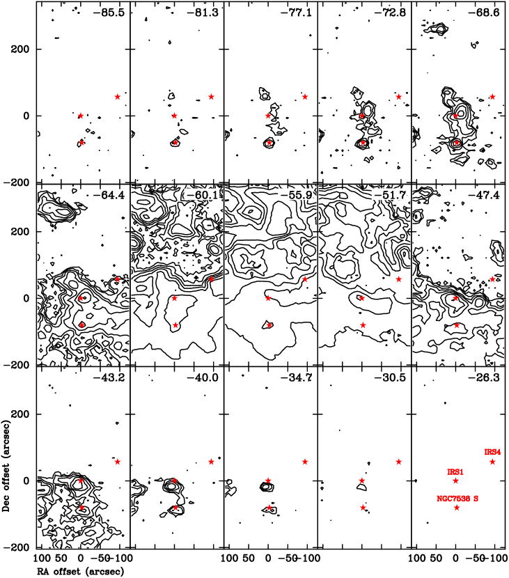
Figure A.1.— Channel maps of CO(3–2) averaged over 4.2 km s^-1 wide velocity intervals. The center velocity of each panel is indicated in the top right corner of each panel. The emission is plotted with eight logarithmic contours from 0.35 K to 26 K. The red stars in each panel are IRS 1, NGC 7538 South and IRS 4. These are labelled in the bottom right panel (velocity -26.3 km s^-1). At high blue- and red-shifted velocities one only sees emission from IRS 1, and NGC 7538 South. IRS 4 is not associated with any outflow. At velocities around -60 km s^-1 we can see the boundary between the NGC 7538 H II region and the molecular could south of it. Emission in the channel at -47 km s^-1 also appears to trace the boundary of the H II region.

Figure A.2.— Channel maps of [C ii] averaged over 3.5 km s^-1 wide velocity intervals. The center velocity of each velocity interval is indicated in the top right corner of each panel. The emission is plotted with ten logarithmic contours from 0.4 K to 40 K. The red stars in each panel are IRS 1, NGC 7538 South. These are labelled in the bottom right panel (velocity -37.0 km s^-1). One can see widespread PDR emission from both the -58 km s^-1 and -50 km s^-1 clouds. NGC 7538 South is not associated with any [C ii] emission. The compact emission NW of NGC 7538 South appears centered on IRS 11, another young early B-star in the cloud.

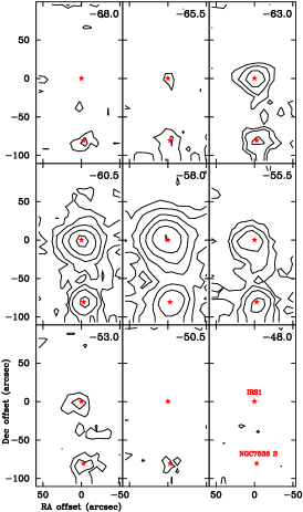
Figure A.3.— Channel maps of CO(11-10) averaged over 2.5 km s^-1 wide velocity intervals. The emission is plotted with six logarithmic contours from 0.5 K to 24 K. The center velocity of each velocity interval is indicated in the top right corner of each panel. The red stars in each panel are IRS 1, NGC 7538 South. These are labelled in the bottom right panel. There is strong CO(11–10) high velocity emission from both IRS 1 and NGC 7538 South. At low velocities, panels -60.5 km s^-1 to -55.5 km s^-1, the CO(11–10) emission extends all the way from IRS 1 to NGC 7538 South. The emission extending to the west from IRS 1, which is seen in panels -60.5 and -58 km s^-1 is almost certainly associated with the NGC 7538 PDR rim.

References

- Akabane & Kuno (2005) Akabane, K., & Kuno, N., 2005, A&A, 431, 183
- Akabane et al. (1992) Akabane, K., Tsunekawa, S., Inoye, M., et al. 1992, PASJ, 44, 435
- Alonso-Martínes et al. (2017) Alonso-Martínes, M., Riviere-Marichalar, P. Meeus, G., et al. 2017, A&A, 603, A138
- Balog et al. (2004) Balog, Z., Kenyon, S. L., Lada, E. A., et al. 2004, AJ, 128, 2942
- Beuther et al. (2017) Beuther, H., Mottram, J. C., Ahmadi, A., et al. 2018, A&A, 617, A100
- Beuther et al. (2017) Beuther, H., Linz, H., & Henning, Th., et al. 2017, A&A, 605, A61
- Beuther, Linz & Henning (2012) Beuther, H., Linz, H., & Henning, Th. 2012, A&A, 543, A88
- Beuther et al. (2002) Beuther, H., Schilke, P., Sridharan, T. K., et al. 2002, A&A, 383, 892
- Buckle et al. (2009) Buckle, J. V., Hills, R. E., Smith, H., et al. 2009, MNRAS, 399, 1026
- Campbell (1984) Campbell, B. 1984, ApJ, 282, L27
- Choi, Evans II & Jaffe (1993) Choi, M., Evans II, N. J., & Jaffe, D. T. 1993, ApJ, 417, 624
- Corder (2008) Corder, S. 2008, PhD thesis, Caltech
- Crampton, Georgelin & Georgelin (1978) Crampton, D., Georgelin, Y. M., & Georgelin, Y. P. 1978, A&A, 66,1
- Davies et al. (2011) Davies, B., Hoare, M. G., Lumsden, S. L., et al. 2011, MNRAS, 416, 972
- Davis et al. (1998) Davis, C. J., Moriarty-Schieven, G., Eislöffel, J., et al. 1998, AJ, 115,1118
- De Buizer & Minier (2005) De Buizer, J. M., & Minier, V. 2005, ApJ, 628, L151
- De Buizer (2003) De Buizer, J. M. 2003, MNRAS, 341, 277
- De Pree et al. (1994) De Pree, C. G., Goss, W. M., Palmer, P., et al. 1994, ApJ, 428, 670
- Fallscheer et al. (2013) Fallscheer, C., Reid, M. A., Di Francesco, J., et al. 2013, ApJ, 773, 102
- Fischer et al. (1985) Fischer, J., Sanders, D. B., Simon, M., et al. 1985, ApJ, 293, 508
- Flower & Pineau des Forêts (2010) Flower, D. R., & Pineau des Forêts, G. 2010,MNRAS, 406, 1745
- Franco-Hernández & Rodríguez (2004) Franco-Hernández, R., & Rodríguez, L. F. 2004, ApJ, 604, L105
- Frau et al. (2014) Frau, P., Girart, J. M., Zhang, Q., et al. 2014, A&A, 567, A116
- Gálvan-Madrid et al. (2010) Galván-Madrid, R., Montes, G., Ramírez, E. A., et al. 2010, ApJ, 713, 423
- Gaume et al. (1995) Gaume, R. A., Goss, W. M., Dickel, H. R., et al. 1995, ApJ, 438, 776
- Goddi, Zhang & Moscadelli (2015) Goddi, C., Zhang, Q., & Moscadelli, L. 2015, A&A, 573, A108
- Goldsmith et al. (2012) Goldsmith, P. F., Langer, W. D., Pineda, J. L., et al. 2012, ApJS, 203,13
- Green et al. (2013) Green, J. D., Evans II, N. J., Jørgensen, J. K., et al. 2013, ApJ, 770, 123
- Hackwell, Grasdalen & Gehrz (1982) Hackwell, J. A., Grasdalen, G. L., and Gehrz, R. D. 1982, ApJ, 252, 250
- Hardebeck (1971) Hardebeck, E. 1971, ApJ, 170, 281
- Herter et al. (2013) Herter, T. L., Vacca. W. D., Adams, J. D., et al. 2013 PASP, 125, 1393
- Herter et al. (2012) Herter, T. L., Adams, J. D., De Buizer, J. M., et al. 2012, ApJ, 749, L18
- Heyminck et al. (2012) Heyminck, S., Graf, U. U., Güsten, R., et al. 2012, A&A, 542, L1
- Hollenbach & Tielens (1999) Hollenbach, D. J., & Tielens, A. G. G. M. 1999, Rev of Modern Physics, 71, 173
- Johnston et al. (2013) Johnston, K. J., Shepherd, D. S., Robitaille, T. P., et al. 2013, A&A, 551, A43
- Kameya et al. (1989) Kameya, O., Hasegawa, T. I., Hirano,, N., et al. 1989, ApJ, 339, 222
- Kauffman et al. (2008) Kauffman, J., Bertoldi, F., Bourke, T. L., et al. 2008, A&A, 487, 993
- van Kempen et al. (2010) van Kempen, T.A., Kristensen, L. E., Herczeg, G. J., et al. 2010, A&A, 518, L121
- Keto et al. (2008) Keto, E., Zhang, Q., & Kurtz, S. 2008, ApJ, 672, 423
- Klaassen et al. (2011) Klaassen, P. D., Wilson, C. D., Keto, E. R., et al. 2011, A&A, 530, A53
- Klaassen et al. (2009) Klaassen, P. D., Wilson, C. D., Keto, E. R., et al. 2009, ApJ, 703, 1308
- Klein et al. (2012) Klein, B., Hochgürtel, S., Krämer, I., et al. 2012, A&A, 542, L3
- Kraus et al. (2006) Kraus, S., Balega, Y., Elitzur, M., et al. 2006, A&A, 455, 521
- Kurtz & Franco (2002) Kurtz, S., & Franco, J. 2002, RevMexAA, 12, 16
- Larson (1978) Larson, R. B. 1978, MNRAS, 184, 69
- Lugo, Lizano & Garay (2004) Lugo, J., Lizano, S., & Garay, G. 2004, ApJ, 614, 807
- Mallick et al. (2014) Mallick, K. K., Ojha, D. K., Tamura, M., et al. 2014, MNRAS, 443, 3218
- Mangum & Shirley (2016) Mangum, J. G., & Shirley, Y. L. 2015, PASP, 127, 266
- Martin (1973) Martin, A. H. M. 1973, MNRAS, 163, 141
- Minier, Booth & Conway (1998) Minier, V., Booth, R. S., & Conway, J. E. 1998, A&A, 336, L5
- Minier, Booth & Conway (2000) Minier, V., Booth, R. S., & Conway, J. E. 2000, A&A, 362, 1093
- Moreno & Chavarría-K (1986) Moreno, M. A., and Chavarría-K, C. 1986, A&A, 161, 130
- Moscadelli et al. (2008) Moscadelli, L., Reid, M. J., Menten, K. M., et al. 2008, ApJ, 693, 406
- Moscadelli & Goddi (2014) Moscadelli, L., & Goddi, C. 2014, A&A, 566, A150
- Mueller et al. (2002) Mueller, K. E., Shirley, Y. M., Evans II, N. J., et al. 2002, ApJS, 143, 469
- Ossenkopf et al. (2015) Ossenkopf, V., Koumpia, E., Okada, Y., et al. 2015, A&A, 580, A83
- Parker, Padman & Scott (1991) Parker, N. D., Padman, R., & Scott, P. F. 1991, MNRAS, 252, 442.
- Pestalozzi et al. (2004) Pestalozzi, M. R., Elitzur, M., Conway, J. E., & Booth, R. S. 2004, ApJ, 603, L113
- Pestalozzi, Elitzur & Conway (2009) Pestalozzi, M. R., Elitzur, M., & Conway, J. E. 2009, A&A, 501, 999
- Podio et al. (2012) Podio, L., Kamp, I., Flower, D., et al. 2012, A&A, 545, A44
- Puga et al. (2010) Puga, E., Marín-Franch, A., Najarro, F., et al. 2010, A&A, 517, A2
- Qiu, Zhang & Menten (2011) Qiu, K., Zhang, Q., & Menten, K. M. 2011, ApJ, 728, 6
- Qiu et al. (2009) Qiu, K., Zhang, Q., Wu, J., et al. 2009, ApJ, 696, 66
- Read (1980) Read, P. L. 1980, MNRAS, 192, 11
- Reynolds (1986) Reynolds, S. P. 1986, ApJ, 304, 713
- Risacher et al. (2016) Risacher, C., Güsten, R., & Stutzki, J., et al. 2016, A&A, 595, A34
- Rodríguez, Anglada & Curiel (1999) Rodríguez, L. F., Anglada, L., & Curiel, S. 1999, ApJS, 125, 427
- Rosero et al. (2019) Rosero, v., Tanaka, K. E. I., Tan, J. C., et al. 2019, ApJ, 873,20
- Sana et al. (2012) Sana, H., de Minck, S. E., de Koter, A., et al. 2012, Science, 337, 44
- Sanna et al. (2018) Sanna, A. Moscadelli, L., Goddi, C., et al. 2018, A&A, 619, A107
- Sanna et al. (2016) Sanna, A. Moscadelli, L., Cesaroni, R., et al. 2016, A&A, 596, L2
- Sandell et al. (2012) Sandell, G., Wright, M., Zhu, L., et al. 2012, ALMA/NAASC 2012 Workshop: Outflows, Winds and Jets (https://science.nrao.edu/facilities/alma/naasc-workshops/jets2012)
- Sandell & Wright (2010) Sandell, G., &Wright, M. 2010, ApJ, 715, 919
- Sandell et al. (2009) Sandell, G., Goss, W. M., Wright, M., & Corder, S. 2009, ApJ, 699, L31
- Sandell, Goss & Wright (2005) Sandell, G., Goss, W. M., & Wright, M. 2005, ApJ, 621, 839
- Sandell & Sievers (2004) Sandell, G., & Sievers, A. 2004, ApJ, 600, 269
- Sault et al. (1995) Sault, R. J., Teuben, P. J., & Wright, M. C. H. 1995, in Astronomical Society of the Pacific Conference Series, Vol. 77, Astronomical Data Analysis Software and Systems IV, ed. R. A. Shaw, H. E. Payne, & J. J. E. Hayes, 433–+
- Sewilo et al. (2004) Sewilo, M., Churchwell, E., Kurtz, S., et al. 2004, ApJ, 605,285
- Scoville et al. (1986) Scoville, N. Z., Sargent, A. I., Claussen, M. J., et al. 1986, ApJ, 303, 416
- Sharma et al. (2017) Sharma, S., Pandey, A. K., Ojha, D. K., et al. 2017, MNRAS, 467, 2965
- Shepherd et al. (1998) Shepherd, D., Watson, A. M., Sargent, A. I., et al. 1998, ApJ, 507, 861
- Surcis et al. (2011) Surcis, G., Vlemmings, W. H. T., Torres, R. M., et al. 2011, A&A, 533, A47
- Tanaka (2017) Tanaka, K. E. I., Tan, J. C., Staff, J. E., et al. 2017, ApJ, 849, 133
- Tanaka,Tan & Zhang (2016) Tanaka, K. E. I., Tan, J. C., & Zhang, Y. 2016, ApJ, 818, 52
- Tielens & Hollenbach (1985) Tielens, A. G. G. M., & Hollenbach, D. J. 1985, ApJ, 291, 722
- Thronson & Harper (1979) Thronson, H. A., Jr, & Harper, D. A. 1979, ApJ, 230, 133
- Visser et al. (2012) Visser, R., Kristensen, L. E., Bruderer, S., et al 2012, A&A, 537, A55
- Wakelam & Herbst (2008) Wakelam, V., & Herbst, E. 2008, ApJ, 680, 371
- Wiesemeyer, Thum & Walmsley (2004) Wiesemeyer, H., Thum, C., & Walmsley, C. M. 2004, A&A, 428, 479
- Willner (1976) Willner, S. P. 1976, ApJ, 206, 728
- Wilson & Rood (1994) Wilson, T. L., & Rood, R. 1994, ARA&A, 32, 191
- Wright et al. (2014) Wright, M. C. H., Hull, C.L. H., Pillai, T., et al. 2014, ApJ, 796, 112
- Wynn-Williams, Becklin, & Neugebauer (1974) Wynn-Williams, C. G., Becklin, E. E., & Neugebauer, G. 1974, ApJ, 187, 473
- Yang et al. (2010) Yang, B., Stancil, P. C., Balakrishnan, N., et al. 2010 ApJ, 218, 1062
- Young et al. (2012) Young, E. T., Becklin, E. E., Marcum, P. M., et al. 2012, ApJ, 749, L17
- Zhang et al. (2019) Zhang, Y., Tanaka, K. E. I., Tan, J. C., et al. 2019, ApJ, 886, L4
- Zhu et al. (2013) Zhu, L., Zhao, J.-H., Wright, M. C. H., et al. 2013, ApJ, 779, 51
- Zhu et al. (2008) Zhu, Q.-F., Lacy, J. F., Jaffe, D. T., et al. 2008, ApJS, 177, 584
- Zinnecker & Yorke (2007) Zinnecker, H., & Yorke, H. W. 2007, Annu. Rev. Astron. Astrophys., 45, 481
- Zinnecker (1982) Zinnecker, H. 1982, NYASA, 395, 226