Nonstationary Reinforcement Learning with Linear Function Approximation

Abstract

We consider reinforcement learning (RL) in episodic Markov decision processes (MDPs) with linear function approximation under drifting environment. Specifically, both the reward and state transition functions can evolve over time, as long as their respective total variations, quantified by suitable metrics, do not exceed certain variation budgets. We first develop the LSVI-UCB-Restart algorithm, an optimistic modification of least-squares value iteration combined with periodic restart, and establish its dynamic regret bound when variation budgets are known. We then propose a parameter-free algorithm, Ada-LSVI-UCB-Restart, that works without knowing the variation budgets, but with a slightly worse dynamic regret bound. We also derive the first minimax dynamic regret lower bound for nonstationary MDPs to show that our proposed algorithms are near-optimal. As a byproduct, we establish a minimax regret lower bound for linear MDPs, which is unsolved by [1]. In addition, we provide numerical experiments to demonstrate the effectiveness of our proposed algorithms. As far as we know, this is the first dynamic regret analysis in nonstationary reinforcement learning with function approximation.

I Introduction

Reinforcement learning (RL) is a core control problem in which an agent sequentially interacts with an unknown environment to maximize its cumulative reward [2]. RL finds enormous applications in real-time bidding in advertisement auctions [3], autonomous driving [4], gaming-AI [5], and inventory control [6], among others. Due to the large dimension of sequential decision-making problems that are of growing interest, classical RL algorithms designed for finite state space such as tabular Q-learning [7] no longer yield satisfactory performance. Recent advances in RL rely on function approximators such as deep neural nets to overcome the curse of dimensionality, i.e., the value function is approximated by a function which is able to predict the value function for unseen state-action pairs given a few training samples. This function approximation technique has achieved remarkable success in various large-scale decision-making problems such as playing video games [8], the game of Go [9], and robot control [10]. Motivated by the empirical success of RL algorithms with function approximation, there is growing interest in developing RL algorithms with function approximation that are statistically efficient [11, 12, 1, 13, 14, 15, 16, 17]. The focus of this line of work is to develop statistically efficient algorithms with function approximation for RL in terms of either regret or sample complexity. Such efficiency is especially crucial in data-sparse applications such as medical trials [18].

However, all of the aforementioned empirical and theoretical works on RL with function approximation assume the environment is stationary, which is insufficient to model problems with time-varying dynamics. For example, consider online advertising. The instantaneous reward is the payoff when viewers are redirected to an advertiser, and the state is defined as the the details of the advertisement and user contexts. If the target users’ preferences are time-varying, time-invariant reward and transition function are unable to capture the dynamics. In general nonstationary random processes naturally occur in many settings and are able to characterize larger classes of problems of interest [19]. Can one design a theoretically sound algorithm for large-scale nonstationary MDPs? In general it is impossible to design algorithm to achieve sublinear regret for MDPs with non-oblivious adversarial reward and transition functions in the worst case [20]. Then what is the maximum nonstationarity a learner can tolerate to adapt to the time-varying dynamics of an MDP with potentially infinite number of states? This paper addresses these two questions.

We consider the setting of episodic RL with nonstationary reward and transition functions. To measure the performance of an algorithm, we use the notion of dynamic regret, the performance difference between an algorithm and the set of policies optimal for individual episodes in hindsight. For nonstationary RL, dynamic regret is a stronger and more appropriate notion of performance measure than static regret, but is also more challenging for algorithm design and analysis. To incorporate function approximation, we focus on a subclass of MDPs in which the reward and transition dynamics are linear in a known feature map [21], termed linear MDP. For any linear MDP, the value function of any policy is linear in the known feature map since the Bellman equation is linear in reward and transition dynamics [1]. Since the optimal policy is greedy with respect to the optimal value function, linear function approximation suffices to learn the optimal policy. For nonstationary linear MDPs, we show that one can design a near-optimal statistically-efficient algorithm to achieve sublinear dynamic regret as long as the total variation of reward and transition dynamics is sublinear. Let $T$ be the total number of time steps, $B$ be the total variation of reward and transition function, $d$ be the ambient dimension of the features, and $H$ be the planning horizon. The contribution of our work is summarized as follows.

• We prove a $\Omega(B^{1/3}d^{2/3}H^{1/3}T^{2/3})$ minimax regret lower bound for nonstationary linear MDP, which shows that it is impossible for any algorithm to achieve sublinear regret on any nonstationary linear MDP with total variation linear in $T$. As a byproduct, we also derive the minimax regret lower bound for stationary linear MDP on the order of $\Omega(\sqrt{dHT})$, which is unsolved in [1].

• We develop the LSVI-UCB-Restart algorithm and analyze the dynamic regret bound for both cases that local variations are known or unknown, assuming the total variations are known. When local variations are known, LSVI-UCB-Restart achieves $\tilde{O}(B^{1/3}d^{4/3}H^{4/3}T^{2/3})$ dynamic regret, which matches the lower bound in $B$ and $T$, up to polylogarithmic factors. When local variations are unknown, LSVI-UCB-Restart achieves $\tilde{O}(B^{1/4}d^{5/4}H^{5/4}T^{3/4})$ dynamic regret.

• We propose a parameter-free algorithm called Ada-LSVI-UCB-Restart, an adaptive version of LSVI-UCB-Restart, and prove that it can achieve $\tilde{O}((B+1)^{1/4}d^{5/4}H^{5/4}T^{3/4})$ dynamic regret without knowing the total variations.

• We conduct numerical experiments on synthetic nonstationary linear MDPs to demonstrate the effectiveness of our proposed algorithms.

I-A Related Work

Nonstationary bandits

Bandit problems can be viewed as a special case of MDP problems with unit planning horizon. It is the simplest model that captures the exploration-exploitation tradeoff, a unique feature of sequential decision-making problems. There are two existing ways to define nonstationarity in the bandit literature. The first one is piecewise-stationary [22], which assumes the expected rewards of arms change in a piecewise manner, i.e., stay fixed for a time period and abruptly change at unknown time steps. The other is to quantify the total variations of expected rewards of arms [23]. The general strategy to adapt to nonstationarity for bandit problems is the forgetting principle: run the algorithm designed for stationary bandits either on a sliding window or in small epochs. This seemingly simple strategy is successful in developing near-optimal algorithms for many variants of nonstationary bandits, such as cascading bandits [24], combinatorial semi-bandits [25] and linear contextual bandits [26, 27]. However, reinforcement learning is much more intricate than bandits. Note that naïvely adapting existing nonstationary bandit algorithms to nonstationary RL leads to regret bounds with exponential dependence on the planing horizon $H$.

RL with function approximation

Motivated by empirical success of deep RL, there is a recent line of work analyzing the theoretical performance of RL algorithms with function approximation, see [11, 12, 1, 13, 14, 15, 16, 17, 28, 29, 30, 31, 32, 33]. All of these works assume that the learner is interacting with a stationary environment, and the learner has access to a realizable or almost realizable function class. In sharp contrast, this paper considers learning in a nonstationary environment. As we will show later, if we do not properly adapt to the nonstationarity, linear regret is incurred.

Nonstationary RL

The last relevant line of work is on dynamic regret analysis of nonstationary MDPs mostly without function approximation [34, 35, 26, 36, 37]. The work of [34] considers the setting in which the MDP is piecewise-stationary and allowed to change in $l$ times for the reward and transition functions. They show that UCRL2 with restart achieves $\tilde{O}((l+1)^{1/3}T^{2/3})$ dynamic regret, where $T$ is the time horizon. Later works [35, 26, 36] generalize the nonstationary setting to allow reward and transition functions vary for any number of time steps, as long as the total variation is bounded. Specifically, the work of [35] proves that UCRL with restart achieves $\tilde{O}((B_{r}+B_{p})^{1/3}T^{2/3})$ dynamic regret, where $B_{r}$ and $B_{p}$ denote the total variation of reward and transition functions over all time steps. One shortcoming of their proposed algorithm is that it requires knowledge of the variation in each epoch. To overcome this issue, [26] proposes an algorithm based on UCRL2, by combining sliding windows and a confidence widening technique. Their algorithm has slightly worse dynamic regret bound $\tilde{O}((B_{r}+B_{p})^{1/4}T^{3/4})$. Further, [36] develops an algorithm which directly optimizes the policy and enjoys near-optimal regret in the low-variation regime. A different model of nonstationary MDP is proposed by [38], which smoothly interpolates between stationary and adversarial environments, by assuming that most episodes are stationary except for a small number of adversarial episodes. Note that [38] considers linear function approximation, but their nonstationarity assumption is different from ours. In this paper, we assume the variation budget for reward and transition function is bounded, which is similar to the settings in [35, 26].

The rest of the paper is organized as follows. After introducing some notations, Sec. II presents our problem definition. Sec. III establishes the minimax regret lower bound for nonstationary linear MDPs. Sec. IV and Sec. V present our algorithms LSVI-UCB-Restart, Ada-LSVI-UCB-Restart and their dynamic regret bounds. Sec. VI shows our experiment results. Sec. VII concludes the paper and discusses some future directions. All detailed proofs can be found in Appendices.

Notation

We use $\langle\cdot,\cdot\rangle$ to denote inner products in Euclidean space, and $\left\lVert\bm{v}\right\rVert_{\Lambda}$ to denote the norm induced by a positive definite matrix $A$ for vector $\bm{v}$, i.e., $\left\lVert\bm{v}\right\rVert_{\Lambda}=\sqrt{\bm{v}^{\top}\Lambda\bm{v}}$. For an integer $N$, we denote the set of positive integers $\{1,2,\ldots,N\}$ as $[N]$.

II Preliminaries

We consider the setting of a nonstationary episodic Markov decision process (MDP), specified by a tuple $(\mathcal{S},\mathcal{A},H,K,\mathbb{P}=\{\mathbb{P}_{h}^{k}\}_{h\in[H],k\in[K]},r=\{r_{h}^{k}\}_{h\in[H],k\in[K]})$, where the set $\mathcal{S}$ is the collection of states, $\mathcal{A}$ is the collection of actions, $H$ is the length of each episode, $K$ is the total number of episodes, and $\mathbb{P}$ and $r$ are the transition kernel and deterministic reward functions respectively. Moreover, $\mathbb{P}_{h}^{k}(\cdot|s,a)$ denotes the transition kernel over the next states if the action $a$ is taken for state $s$ at step $h$ in the $k$-th episode, and $r_{h}^{k}:\mathcal{S}\times\mathcal{A}\rightarrow[0,1]$ is the deterministic reward function at step $h$ in the $k$-th episode. Note that we are considering a nonstationary setting, thus we assume the transition kernel $\mathbb{P}$ and reward function $r$ may change in different episodes. We will explicitly quantify the nonstationarity later.

The learning protocol proceeds as follows. In episode $k$, the initial state $s_{1}^{k}$ is chosen by an adversary. Then at each step $h\in[H]$, the agent observes the current state $s_{h}\in\mathcal{S}$, takes an action $a_{h}\in\mathcal{A}$, receives an instantaneous reward $r_{h}^{k}(s_{h},a_{h})$, then transitions to the next state $s_{h+1}$ according to the distribution $\mathbb{P}_{h}^{k}(\cdot|s_{h},a_{h})$. This process terminates at step $H$ and then the next episode begins. The agent interacts with the environment for $K$ episodes, which yields $T=KH$ time steps in total.

A policy $\pi$ is a collection of functions $\pi_{h}:\mathcal{S}\rightarrow\mathcal{A},\forall h\in[H]$. We define the value function at step $h$ in the $k$-th episode for policy $\pi$ as the expected value of the cumulative rewards received under policy $\pi$ when starting from an arbitrary state $s$:

$$V^{\pi}_{h,k}(s)=\mathbb{E}_{\pi}\left[\sum_{h^{\prime}=h}^{H}r_{h^{\prime}}^{k}(s_{h^{\prime}},a_{h^{\prime}})|s_{h}=s\right],\forall s\in\mathcal{S},h\in[H],k\in[K].$$

Note that the value function also depends on the episode $k$ since the Markov decision process is nonstationary. Similarly, we can also define the action-value function (a.k.a. $Q$ function) for policy $\pi$ at step $h$ in the $k$-th episode, which gives the expected cumulative reward starting from an arbitrary state-action pair:

$$Q^{\pi}_{h,k}(s,a)=r_{h}^{k}(s,a)+\mathbb{E}_{\pi}\left[\sum_{h^{\prime}=h+1}^{H}r_{h^{\prime}}^{k}(s_{h^{\prime}},a_{h^{\prime}})|s_{h}=s,a_{h}=a\right],\forall(s,a)\in\mathcal{S}\times\mathcal{A},h\in[H],k\in[K].$$

We define the optimal value function and optimal action-value function for step $h$ in $k$-th episode as $V^{*}_{h,k}(s)=\sup_{\pi}V^{\pi}_{h,k}(s)$ and $Q^{*}_{h,k}(s,a)=\sup_{\pi}Q^{\pi}_{h,k}(s,a)$ respectively, which always exist [39]. For simplicity, we denote $\mathbb{E}_{s^{\prime}\sim\mathbb{P}_{h}^{k}(\cdot|s,a)}[V_{h+1}(s^{\prime})]=[\mathbb{P}_{h}^{k}V_{h+1}](s,a)$. Using this notation, we can write down the Bellman equation for any policy $\pi$,

$$Q_{h,k}^{\pi}(s,a)=(r_{h}^{k}+\mathbb{P}_{h}^{k}V_{h+1,k}^{\pi})(s,a),V_{h,k}^{\pi}(s)=Q_{h,k}^{\pi}(s,\pi_{h}(s)),V_{H+1,k}^{\pi}(s)=0,\forall(s,a,k)\in\mathcal{S}\times\mathcal{A}\times[K].$$

Similarly, the Bellman optimality equation is

$$Q_{h,k}^{*}(s,a)=(r_{h}^{k}+\mathbb{P}_{h}^{k}V_{h+1,k}^{*})(s,a),V_{h,k}^{*}(s)=\max_{a\in\mathcal{A}}Q_{h,k}^{*}(s,a),V_{H+1,k}^{*}(s)=0,\forall(s,a,k)\in\mathcal{S}\times\mathcal{A}\times[K].$$

This implies that the optimal policy $\pi^{*}$ is greedy with respect to the optimal action-value function $Q^{*}(\cdot,\cdot)$. Thus in order to learn the optimal policy it suffices to estimate the optimal action-value function.

Recall that the agent is learning the optimal policy via interactions with the environment, despite the uncertainty of $r$ and $\mathcal{P}$. In the $k$-th episode, the adversary chooses the initial state $s_{1}^{k}$, then the agent decides its policy $\pi^{k}$ for this episode based on historical interactions. To measure the convergence to optimality, we consider an equivalent objective of minimizing the dynamic regret [40, 1],

$$\text{Dyn-Reg}(K)=\sum_{k=1}^{K}\left[V^{*}_{1,k}(s_{1}^{k})-V^{\pi^{k}}_{1,k}(s_{1}^{k})\right].$$

II-A Linear Markov Decision Process

We consider a special class of MDPs called linear Markov decision process [21, 41, 1], which assumes both transition function $\mathbb{P}$ and reward function $r$ are linear in a known feature map $\bm{\phi}(\cdot,\cdot)$. The formal definition is as follows.

Definition 1.

(Linear MDP). The MDP $(\mathcal{S},\mathcal{A},H,K,\mathbb{P},r)$ is a linear MDP with the feature map $\bm{\phi}:\mathcal{S}\times\mathcal{A}\rightarrow\mathbb{R}^{d}$, if for any $(h,k)\in[H]\times[K]$, there exist $d$ unknown measures $\bm{\mu}_{h,k}=(\bm{\mu}_{h,k}^{1},\ldots,\bm{\mu}_{h,k}^{d})^{\top}$ on $\mathcal{S}$ and a vector $\bm{\theta}_{h,k}\in\mathbb{R}^{d}$ such that

$$\mathbb{P}_{h}^{k}(s^{\prime}|s,a)=\bm{\phi}(s,a)^{\top}\bm{\mu}_{h,k}(s^{\prime}),\quad r_{h}^{k}(s,a)=\bm{\phi}(s,a)^{\top}\bm{\theta}_{h,k}.$$

Without loss of generality, we assume $\left\lVert\bm{\phi}(s,a)\right\rVert\leq 1$ for all $(s,a)\in\mathcal{S}\times\mathcal{A}$, and $\max\{\left\lVert\bm{\mu}_{h,k}\right\rVert,\left\lVert\bm{\theta}_{h,k}\right\rVert\}\leq\sqrt{d}$ for all $(h,k)\in[H]\times[K]$.

Note that the transition function $\mathbb{P}$ and reward function $r$ are determined by the unknown measures $\{\bm{\mu}_{h,k}\}_{h\in[H],k\in[K]}$ and latent vectors $\{\bm{\theta}_{h,k}\}_{h\in[H],k\in[K]}$. The quantities $\bm{\mu}_{h,k}$ and $\bm{\theta}_{h,k}$ vary across time in general, which leads to change in transition function $\mathbb{P}$ and reward function $r$. Following [23, 26, 40], we quantify the total variation on $\bm{\mu}$ and $\bm{\theta}$ in terms of their respective variation budget $B_{\bm{\theta}}$ and $B_{\bm{\mu}}$, and define the total variation budget $B$ as the summation of these two variation budgets:

$$B_{\bm{\theta}}=\sum_{k=2}^{K}\sum_{h=1}^{H}\left\lVert\bm{\theta}_{h,k}-\bm{\theta}_{h,k-1}\right\rVert_{2},\quad B_{\bm{\mu}}=\sum_{k=2}^{K}\sum_{h=1}^{H}\left\lVert\bm{\mu}_{h,k}-\bm{\mu}_{h,k-1}\right\rVert_{\text{F}},\quad B=B_{\bm{\theta}}+B_{\bm{\mu}}\mbox{.}$$

III Minimax Regret Lower Bound

In this section, we derive the minimax regret lower bound for nonstationary linear MDPs. All of the detailed proofs for this section are included in Appendix A.

We first derive the minimax regret lower bound for stationary linear MDP by constructing hard instances, which addresses a problem proposed in [1].

Theorem 1.

For any algorithm, if $d\geq 4$ and $T\geq 64(d-3)^{2}H$, then there exists at least one stationary linear MDP instance that incurs regret at least $\Omega(d\sqrt{HT})$.

Remark 1.

Note that this lower bound is tighter than simply applying the minimax regret lower bound for tabular episodic MDP. Recall that the minimax regret lower bound for tabular episodic MDP is $\Omega(\sqrt{SAHT})$ [42], and we can convert any tabular MDP into a linear MDP by setting the feature $\bm{\phi}(\cdot,\cdot)$ as an indicator vector with $d=SA$ dimension [1]. Thus simply applying the regret lower bound for tabular episodic MDP yields $\Omega\left(\sqrt{dHT}\right)$.

The key step of this proof is to construct the hard-to-learn MDP instances. Inspired by lower bound construction for stochastic contextual bandits [43, 44], we construct an ensemble of hard-to-learn 3-state linear MDPs, which is illustrated in Fig. 1.

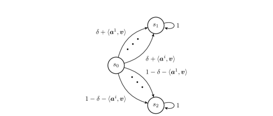
Figure 1: Graphical illustration of the hard-to-learn linear MDP instances with deterministic reward.

Each linear MDP instance in this ensemble has three states $s_{0},s_{1},s_{2}$ ($s_{1}$ and $s_{2}$ are absorbing states), and it is characterized by a unique $(d-3)$-dimensional vector $\{\pm\sqrt{(d-3)H}/\sqrt{T}\}^{d-3}$. Specifically, the vector $\bm{v}$ defines the transition function of the corresponding MDP, as illustrated in Fig. 1. Each action $a$ of this MDP instance is encoded by a $(d-3)$ dimensional vector $\bm{a}\in\left\{\pm 1/\sqrt{d-3}\right\}^{d-3}$. The reward functions for the three states are fixed regardless of the actions, specifically, $r(s_{0},a)=r(s_{2},a)=0,r(s_{1},a)=1,\forall a\in\mathcal{A}$. For each episode, the agent starts at $s_{0}$, and ends at step $H$. The transition functions of the linear MDP parametrized by $\bm{v}$ are defined as follows,

$$\mathbb{P}(s_{1}|s_{0},a)=\delta+\langle\bm{a},\bm{v}\rangle,\quad\mathbb{P}(s_{2}|s_{0},a)=1-\delta-\langle\bm{a},\bm{v}\rangle,$$

$$\mathbb{P}(s_{1}|s_{1},a)=1,\quad\mathbb{P}(s_{2}|s_{2},a)=1,$$

where $\delta=\frac{1}{4}$. Notice that the optimal policy for the MDP instance parametrized by $\bm{v}$ is taking the action that maximizes the probability to reach $s_{1}$, which is equivalent to taking the action such that its corresponding vector $\bm{a}$ satisfies $\text{sgn}(\bm{a}_{i})=\text{sgn}(\bm{v}_{i}),\forall i\in[d-3]$. Furthermore, it can be verified that the above MDP instance is indeed a linear MDP, by setting:

$$\bm{\phi}(s_{0},a)=(0,1,\delta,\bm{a}),\bm{\phi}(s_{1},a)=(1,0,0,\vec{0}),\bm{\phi}(s_{2},a)=(0,1,0,\vec{0})$$

$$\bm{\mu}(s_{0})=(0,0,0,\vec{0}),\bm{\mu}(s_{1})=(1,0,1,\bm{v}),\bm{\mu}(s_{2})=(0,1,-1,-\bm{v}),\bm{\theta}=(1,0,0,0).$$

Remark 2.

Note that the above parameters violate the normalization assumption in Def. 1, but it is straightforward to normalize them. We ignore the additional rescaling to clarify the presentation.

After constructing the ensemble of hard instances, we can derive the minimax regret lower bound for stationary linear MDP. For the detailed proof, please refer to Appendix A.

Based on Thm. 1, we can derive the dynamic regret lower bound for nonstationary linear MDP

Theorem 2.

For any algorithm, the dynamic regret is at least $\Omega(B^{1/3}d^{2/3}H^{1/3}T^{2/3})$ for one nonstationary linear MDP instance, if $d\geq 4$, $64(d-3)^{2}H$.

Sketch of Proof.

The construction of the lower bound instance is based on the construction used in Thm. 1. Nature divides the whole time horizon into $\lceil\frac{K}{N}\rceil$ intervals of equal length $N$ episodes (the last episode may be shorter). For each interval, nature initiates a new stationary linear MDP parametrized by $\bm{v}$, which is drawn from a set $\{\pm\sqrt{d-3}/{\sqrt{N}}\}^{d-3}$. Note that nature chooses the parameters for the linear MDP for each interval only depending on the learner’s policy, and the worst-case regret for each interval is at least $\Omega(d\sqrt{H^{2}N})$. Since there are at least $\lceil\frac{K}{N}\rceil-1$ intervals, the total regret is at least $\Omega(d\sqrt{H^{2}K^{2}}N^{-1/2})$. By checking the total variation budget $B$, we can obtain the lower bound for $L$, which is $\Omega(B^{-2/3}d^{2/3}K^{2/3})$. Then we can obtain the desired regret lower bound. For the detailed proof, please refer to Appendix A. ∎

We can use the same proof technique to derive the minimax regret lower bound for tabular MDPs, which have not been solved in [40, 35]. In general if we only care about the total variation $B$ and the time horizion $T$, the minimax dynamic regret lower bound for reinforcement learning is $\Omega(B^{1/3}T^{2/3})$, which also agrees with the result from nonstationary bandits [23, 26]. Recall that for infinite-horizon average-reward tabular MDP, the variation budgets are defined as $B_{r}=\sum_{t=1}^{T-1}\max_{s,a}|r_{t+1}(s,a)-r_{t}(s,a)|$, $B_{p}=\sum_{t=1}^{T-1}\max_{s,a}\left\lVert p_{t+1}(\cdot|s,a)-p_{t}(\cdot|s,a)\right\rVert_{1}$ [40]. We further define the total variation budget as $B=B_{p}+B_{r}$. The diameter of a MDP $M$ is defined as $D(M)=\min_{s,s^{\prime}}\max_{\pi}\mathbb{E}[T(s^{\prime}|M,s,\pi)]$, where $T(s^{\prime}|M,s,\pi)$ is the random variable for the first time step in which state $s^{\prime}$ is reached when the agent starts at state $s$ and plays policy $\pi$ [34]. Let $D_{\max}=\max_{t}D_{t}$, the maximum diameter. The minimax dynamic regret lower bound for nonstationary infinite-horizion average-reward tabular MDP is presented in the following corollary.

Corollary 1.

For any algorithm, if $S\geq 10$, $A\geq 10$, $D_{\max}\geq 20\log_{A}S$, and $T\geq DSA$, there is a nonstationary MDP instance with $S$ states, $A$ actions and maximum diameter $D_{\max}$, such that the dynamic regret is lower bounded by $\Omega(D_{\max}^{2/3}B^{1/3}S^{1/3}A^{1/3}T^{2/3})$.

The high-level proof strategy is similar to the one used in Thm. 2, and the key difference is the lower bound construction. For the detailed proof, please refer to Appendix A.

IV LSVI-UCB-Restart Algorithm

In this section, we describe our proposed algorithm LSVI-UCB-Restart, and discuss how to tune the hyper-parameters for cases when local variation is known or unknown. For both cases, we present their respective regret bounds. Detailed proofs are deferred to Appendix B.

IV-A Algorithm Description

Our proposed algorithm LSVI-UCB-Restart has two key ingredients: least-squares value iteration with upper confidence bound to properly handle the exploration-exploitation trade-off [1], and restart strategy to adapt to the unknown nonstationarity. The algorithm is summarized in Alg. 1. From a high-level point of view, our algorithm runs in epochs. At each epoch, we first estimate the action-value function by solving a regularized least-squares problem from historical data, then construct the upper confidence bound for the action-value function, and update the policy greedily w.r.t. action-value function plus the upper confidence bound. Finally, we periodically restart our algorithm to adapt to the nonstationary nature of the environment.

Next, we delve into more details of the algorithm design. As a preliminary, we briefly introduce least-squares value iteration [41, 45], which is the key tool to estimate $\bm{w}$, the latent vector used to form the optimal action-value function, $Q^{*}_{h,k}(\cdot,\cdot)=\langle\bm{\phi}(\cdot,\cdot),\bm{w}\rangle$. Least-squares value iteration is a natural extension of classical value iteration algorithm  [2], which finds the optimal action-value function by recursively applying Bellman optimality equation,

$$Q_{h,k}^{*}(s,a)=[r_{h,k}+\mathbb{P}_{h}^{k}\max_{a^{\prime}\in\mathcal{A}}Q_{h+1,k-1}^{*}(\cdot,a^{\prime})](s,a).$$

In practice, the transition function $\mathbb{P}$ is unknown, and the state space might be so large that it is impossible for the learner to fully explore all states. If we parametrize the action-value function in a linear form as $\langle\bm{\phi}(\cdot,\cdot),\bm{w}\rangle$, it is natural to solve a regularized least-squares problems using collected data inspired by classical value iteration. Specifically, the update formula of $\bm{w}_{h}^{k}$ in Alg. 1 (line 8) is the analytic solution of the following regularized least-squares problem:

$$\bm{w}_{h}^{k}=\arg\min_{\bm{w}}\sum_{l=\tau}^{k-1}[r_{h,l}(s_{h}^{l},a_{h}^{l})+\max_{a\in\mathcal{A}}Q_{h+1}^{k-1}(s_{h+1}^{l},a)-\langle\bm{\phi}(s_{h}^{l},a_{h}^{l}),\bm{w}\rangle]^{2}+\left\lVert\bm{w}\right\rVert_{2}.$$

One might be skeptical since simply applying least-squares method to solve $\bm{w}$ does not take the distribution drift in $\mathbb{P}$ and $r$ into account and hence, may lead to non-trivial estimation error. However, we show that the estimation error can gracefully adapt to the nonstationarity, and it suffices to restart the estimation periodically to achieve good dynamic regret.

In addition to least-squares value iteration, the inner loop of Alg. 1 also adds an additional quadratic bonus term $\beta\left\lVert\bm{\phi}(\cdot,\cdot)\right\rVert_{(\Lambda^{k}_{h})^{-1}}$ (line 9) to encourage exploration, where $\beta$ is a scalar and $\Lambda^{k}_{h}$ is the Gram matrix of the regularized least-squares problem. Intuitively, $1/\left\lVert\bm{\phi}\right\rVert_{(\Lambda^{k}_{h})^{-1}}^{-1}$ is the effective sample number of the agent observed so far in the direction of $\bm{\phi}$, thus the quadratic bonus term can quantify the uncertainty of estimation. We will show later if we tune $\beta_{k}$ properly, then our action-value function estimate $Q_{h}^{k}$ can be an optimistic upper bound or an approximately optimistic upper bound of the optimal action-value function, so we can adapt the principle of optimism in the face of uncertainty [46] to explore.

Finally, we use epoch restart strategy to adapt to the drifting environment, which achieves near-optimal dynamic regret notwithstanding its simplicity. Specifically, we restart the estimation of $\bm{w}$ after $\frac{W}{H}$ episodes, all illustrated in the outer loop of Alg. 1. Note that in general epoch size $W$ can vary for different epochs, but we find that a fixed length is sufficient to achieve near-optimal performance.

Algorithm 1 LSVI-UCB-Restart Algorithm

0:  time horizon $T$, epoch size $W$

1:  Set epoch counter $j=1$.

2:  while $j\leq\lceil\frac{T}{W}\rceil$ do

3:     set $\tau=(j-1)\frac{W}{H}$

4:     for all $k=\tau,\tau+1,\ldots,\min(\tau+\frac{W}{H}-1,K)$ do

5:        Receive the initial state $s^{k}_{1}$.

6:        for all step $h=H,\ldots,1$ do

7:           $\Lambda_{h}^{k}\leftarrow\sum_{l=\tau}^{k-1}\bm{\phi}(s_{h}^{l},a_{h}^{l})\bm{\phi}(s_{h}^{l},a_{h}^{l})^{\top}+I$

8:           $\bm{w}_{h}^{k}\leftarrow(\Lambda_{h}^{k})^{-1}\sum_{l=\tau}^{k-1}\bm{\phi}(s_{h}^{l},a_{h}^{l})[r_{h,l}(s_{h}^{l},a_{h}^{l})+\max_{a}Q_{h+1}^{k-1}(s^{l}_{h+1},a)]$

9:           $Q_{h}^{k}(\cdot,\cdot)\leftarrow\min\{(\bm{w}_{h}^{k})^{\top}\bm{\phi}(\cdot,\cdot)+\beta_{k}\left\lVert\bm{\phi}(\cdot,\cdot)\right\rVert_{(\Lambda^{k}_{h})^{-1}},H\}$

10:        end for

11:        for all step $h=1,\ldots,H$ do

12:           take action $a_{h}^{k}\leftarrow\arg\max_{a}Q_{h}^{k}(s_{h}^{k},a)$, and observe $s_{h+1}^{k}$

13:        end for

14:     end for

15:     set $j=j+1$

16:  end while

IV-B Regret Analysis

Now we derive the dynamic regret bounds for LSVI-UCB-Restart, first introducing additional notation for local variations. We let $B_{\bm{\theta},\mathcal{E}}=\sum_{k\in\mathcal{E}}\sum_{h=1}^{H}\left\lVert\bm{\theta}_{h,k}-\bm{\theta}_{h,k-1}\right\rVert_{2}$ and $B_{\bm{\mu},\mathcal{E}}=\sum_{k\in\mathcal{E}}\sum_{h=1}^{H}\left\lVert\bm{\mu}_{h,k}-\bm{\mu}_{h,k-1}\right\rVert_{\text{F}}$ be the local variation for $\bm{\theta}$ and $\bm{\mu}$ in epoch $\mathcal{E}$. To derive the dynamic regret lower bounds, we need the following lemma to control the fluctuation of least-squares value iteration.

Lemma 1.

(Modified from [1]) Denote $\tau$ to be the first episode in the epoch which contains episode $k$. There exists an absolute constant $C$ such that the following event $E$,

$$\left\lVert\sum_{l=\tau}^{k-1}\bm{\phi}_{h}^{l}[V_{h+1}^{k}(s^{l}_{h+1})-\mathbb{P}_{h}^{l}V_{h+1}^{k}(s_{h}^{l},a_{h}^{l})]\right\rVert_{(\Lambda_{h}^{k})^{-1}}\leq CdH\sqrt{\log[2(c_{\beta}+1)dW/p]},\quad\forall(k,h)\in\mathcal{E}\times[H].$$

happens with probability at least $1-p/2$.

Next we proceed to derive the dynamic regret bounds for two cases: (1) local variations are known, and (2) local variations are unknown.

Known Local Variations

For the case of known local variations, under event $E$ defined in Lemma 1, the estimation error of least-squares estimation scales with the quadratic bonus $\left\lVert\bm{\phi}(\cdot,\cdot)\right\rVert_{(\Lambda^{k}_{h})^{-1}}$ uniformly for any policy $\pi$, which is detailed in the following lemma.

Lemma 2.

Under event $E$ defined in Lemma 1, we have for any policy $\pi$, $\forall s,a,h,k\in\mathcal{S}\times\mathcal{A}\times[H]\times\mathcal{E}$,

$$|\langle\bm{\phi}(s,a),\bm{w}_{h}^{k}\rangle-Q^{\pi}_{h,k}(s,a)-\mathbb{P}_{h}^{k}(V^{k}_{h+1}-V^{\pi}_{h+1,k})(s,a)|\leq\beta_{k}\left\lVert\bm{\phi}(s,a)\right\rVert_{(\Lambda^{k}_{h})^{-1}},$$

where $\beta_{k}=C_{0}dH\sqrt{\log(2dW/p)}+B_{\bm{\theta},\mathcal{E}}\sqrt{d(k-\tau)}+B_{\bm{\mu},\mathcal{E}}H\sqrt{d(k-\tau)}$ and $\tau$ is the first episode in the current epoch.

The proof of Lemma 2 is included in Appendix B. Based on Lemma 2, we can show that if we set $\beta_{k}$ properly with knowledge of local variations $B_{\bm{\theta},\mathcal{E}}$ and $B_{\bm{\mu},\mathcal{E}}$, the action-value function estimate maintained in Alg. 1 is an upper bound of the optimal action-value function under event $E$.

Lemma 3.

Under event $E$ defined in Lemma 1, for episode $k$, if we set $\beta_{k}=cdH\sqrt{\log(2dW/p)}+B_{\bm{\theta},\mathcal{E}}\sqrt{d(k-\tau)}+B_{\bm{\mu},\mathcal{E}}H\sqrt{d(k-\tau)}$, we have

$$Q^{k}_{h}(s,a)\geq Q^{*}_{h,k},\quad\forall(s,a,h,k)\in\mathcal{S}\times\mathcal{A}\times[H]\times\mathcal{E}.$$

Sketch of Proof.

For the last step $H$ in each episode, the results hold due to Lemma 2 since after step $H$ there is no reward and the episode terminates. We then prove $Q_{h}^{k}$ is indeed the upper bound for the optimal action-value function $Q^{*}_{h,k}$ for remaining $h\in[H-1]$ by induction. Please see Appendix B for details. ∎

After showing the action-value function estimate is the optimistic upper bound of the optimal action-value function, we can derive the dynamic regret bound within one epoch via recursive regret decomposition. The dynamic regret within one epoch for Alg. 1 with the knowledge of $B_{\bm{\theta},\mathcal{E}}$ and $B_{\bm{\mu},\mathcal{E}}$ is as follows.

Theorem 3.

For each epoch $\mathcal{E}$ with epoch size $W$, set $\beta$ in the $k$-th episode as $\beta_{k}=cdH\sqrt{\log(2dW/p)}+B_{\bm{\theta},\mathcal{E}}\sqrt{d(k-\tau)}+B_{\bm{\mu},\mathcal{E}}H\sqrt{d(k-\tau)}$, where $c$ is an absolute constant and $p\in(0,1)$. Then the dynamic regret within that epoch is $\tilde{O}(H^{3/2}d^{3/2}W^{1/2}+B_{\bm{\theta},\mathcal{E}}dW+B_{\bm{\mu},\mathcal{E}}dHW)$ with probability at least $1-p$.

Proof.

See Appendix B. ∎

By summing over all epochs and applying the union bound, we can obtain the dynamic regret upper bound for LSVI-UCB-Restart for the whole time horizon.

Theorem 4.

If we set $\beta_{k}=cdH\sqrt{\log(2dT/p)}+B_{\bm{\theta},\mathcal{E}}\sqrt{d(k-\tau)}+B_{\bm{\mu},\mathcal{E}}H\sqrt{d(k-\tau)}$, the dynamic regret of LSVI-UCB-Restart is $\tilde{O}(H^{3/2}d^{3/2}TW^{-1/2}+B_{\bm{\theta}}dW+B_{\bm{\mu}}dHW)$, with probability at least $1-p$.

By properly tuning the epoch size $W$, we can obtain a tight dynamic regret upper bound.

Corollary 2.

Let $W=\lceil B^{-2/3}T^{2/3}d^{1/3}H^{-2/3}\rceil H$, and $\beta_{k}=cdH\sqrt{\log(2dW/p)}+B_{\bm{\theta},\mathcal{E}}\sqrt{d(k-\tau)}+B_{\bm{\mu},\mathcal{E}}H\sqrt{d(k-\tau)}$ for each epoch. LSVI-UCB-Restart achieves $\tilde{O}(B^{1/3}d^{4/3}H^{4/3}T^{2/3})$ dynamic regret, with probability at least $1-p$.

Remark 3.

Corollary 2 shows that if local variations are known, we can achieve near-optimal dependency on the the total variation $B_{\bm{\theta}},B_{\bm{\mu}}$ and time horizon $T$ compared to the lower bound provided in Thm 2. However, the dependency on $d$ and $H$ is worse. This is not surprising since the dependency on $d$ and $H$ is not optimal for LSVI-UCB suggested by Thm 1, thus it is impossible for LSVI-UCB-Restart to achieve optimal dependency on $d$ and $H$.

Unknown Local Variation

If the local variations are unknown, the proof is similar to the case of known local variations. We only highlight the differences compared to the previous case. The key difference is that without knowledge of local variations $B_{\bm{\theta}}$ and $B_{\bm{\mu}}$, we set the hyper-parameter $\beta=cdH\sqrt{\log(2dW/p)}$. As a result, the action-value function estimate $Q_{h}^{k}$ maintained in Alg. 1 is no longer the optimistic upper bound of the optimal action-value function, but only approximately, up to some error, proportional to the local variation. The rigorous statement is as follows.

Lemma 4.

Under event $E$ defined in Lemma 1, if we set $\beta=cdH\sqrt{\log(2dW/p)}$, we have

$$\forall(s,a,h,k)\in\mathcal{S}\times\mathcal{A}\times[H]\times\mathcal{E},$$

$$Q^{k}_{h}(s,a)\geq Q^{*}_{h,k}-(H-h+1)(B_{\bm{\theta},\mathcal{E}}\sqrt{d(k-\tau)}+B_{\bm{\mu},\mathcal{E}}H\sqrt{d(k-\tau)}).$$

Sketch of Proof.

For the case when local variations are unknown, the least -squares estimation error have some additional terms that are linear in the local variations $B_{\bm{\theta},\mathcal{E}}$ and $B_{\bm{\mu},\mathcal{E}}$ (See Lemma 7 in Appendix B). Then we can prove that $Q_{h}^{k}$ is an approximate upper bound of $Q^{*}_{h,k}$ via induction. For details, please see Appendix B. ∎

By applying a similar proof technique as Thm. 3, we can derive the dynamic regret within one epoch when local variations are unknown.

Theorem 5.

For each epoch $\mathcal{E}$ with epoch size $W$, if we set $\beta_{k}=cdH\sqrt{\log(2dW/p)}$, where $c$ is an absolute constant and $p\in(0,1)$, then the dynamic regret within that epoch is $\tilde{O}(\sqrt{d^{3}H^{3}W}+B_{\bm{\theta},\mathcal{E}}\sqrt{d/H}W^{3/2}+B_{\bm{\mu},\mathcal{E}}\sqrt{dH}W^{3/2})$ with probability at least $1-p$, where $B_{\bm{\theta},\mathcal{E}}$ and $B_{\bm{\mu},\mathcal{E}}$ are the total variation within that epoch.

By summing regret over epochs and applying a union bound over all epochs, we obtain the dynamic regret of LSVI-UCB-Restart for the whole time horizon.

Theorem 6.

If we set $\beta=cdH\sqrt{\log(2dT/p)}$, then the dynamic regret of LSVI-UCB-Restart is $\tilde{O}(d^{3/2}H^{3/2}TW^{-1/2}+B_{\bm{\theta}}d^{1/2}H^{-1/2}W^{3/2}+B_{\bm{\mu}}d^{1/2}H^{1/2}W^{3/2})$, with probability at least $1-p$.

Note that in this case the tuning is exactly the same as in [1], which is designed to learn the optimal policy in a stationary linear MDP. This result is in sharp contrast with nonstationary linear contextual bandits [26, 27], where the nonstationarity can incur linear regret if the total variation is $\Omega(1)$ and the learner does not properly adapt to the nostationarity. Our analysis shows that for episodic reinforcement learning, the nonstationarity can incur linear regret as long as total variation is $\Omega(T^{-1/2})$ if the learner is unaware of it. The reason is that in episodic reinforcement learning, the learner aims to learn a policy that maximizes the total reward over a long horizon, and the distribution shift in the environment can propagate through the whole episode to increase the estimation error. As a result, the learner is more sensitive to drift in environment. This illustrates the hardness of planning over long horizon from another perspective. By properly tuning the epoch size $W$, we can obtain a tight regret bound for the case of unknown local variations as follows.

Corollary 3.

Let $W=\lceil B^{-1/2}T^{1/2}d^{1/2}H^{1/2}\rceil H$ and $\beta_{k}=cdH\sqrt{\log(2dW/p)}$. Then LSVI-UCB-Restart achieves $\tilde{O}(B^{1/4}d^{5/4}H^{5/4}T^{3/4})$ dynamic regret, with probability at least $1-p$.

Corollary 4.

Let $W=\lceil T^{1/2}d^{1/2}H^{1/2}\rceil H$, $\beta_{k}=cdH\sqrt{\log(2dW/p)}$, LSVI-UCB-Restart achieves $\tilde{O}(Bd^{5/4}H^{5/4}T^{3/4})$ dynamic regret, with probability at least $1-p$.

V Ada-LSVI-UCB-Restart: a Parameter-free Algorithm

In practice, the total variations $B_{\bm{\theta}}$ and $B_{\bm{\mu}}$ are unknown. To mitigate this issue, we present a parameter-free algorithm Ada-LSVI-UCB-Restart and its dynamic regret bound.

V-A Algorithm Description

Inspired by bandit-over-bandit mechanism [26], we develop a new parameter-free algorithm. The key idea is to use LSVI-UCB-Restart as a subroutine (set $\beta=cdH\sqrt{\log(2dT/p)}$ since we assume total variations are unknown), and periodically update the epoch size based on the historical data under the time-varying $\mathbb{P}$ and $r$ (potentially adversarial). More specifically, Ada-LSVI-UCB-Restart (Alg. 2) divides the whole time horizon into $\lceil\frac{T}{HM}\rceil$ blocks of equal length $M$ episodes (the length of the last block can be smaller than $M$ episodes), and specifies a set $J_{W}$ from which epoch size is drawn. For each block $i\in[\lceil\frac{T}{HM}\rceil]$, Ada-LSVI-UCB runs a master algorithm to select the epoch size $W_{i}$ and runs LSVI-UCB-Restart with $W_{i}$ for the current block. After the end of this block, the total reward of this block is fed back to the master algorithm, and the posteriors of the parameters are updated accordingly.

For the detailed master algorithm, we select EXP3-P [47] since it is able to deal with non-oblivious adversary. Now we present the details of Ada-LSVI-UCB-Restart. We set the length of each block $M$ and the feasible set of epoch size $J_{W}$ as follows:

$$M=\lceil 5T^{1/2}d^{1/2}H^{1/2}\rceil,J_{W}=\{H,2H,\ldots,MH\}.$$

The intuition of designing the feasible set for epoch size $J_{W}$ is to guarantee it can well-approximate the optimal epoch size with the knowledge of total variations while on the other hand make it as small as possible, so the learner do not lose much by adaptively selecting the epoch size from $J_{W}$. This intuition is more clear when we derive the dynamic regret bound of Ada-LSVI-UCB-Restart. Denoting $|J_{W}|=\Delta$, the master algorithm EXP3-P treats each element of $J_{W}$ as an arm and updates the probabilities of selecting each feasible epoch size based on the reward collected in the past. It begins by initializing

$$\alpha=0.95\sqrt{\frac{\ln\Delta}{\Delta\lceil T/MH\rceil}},\beta=\sqrt{\frac{\ln\Delta}{\Delta\lceil T/MH\rceil}},$$ (1)

$$\gamma=1.05\sqrt{\frac{\ln\Delta}{\Delta\lceil T/MH\rceil}},q_{l,1}=0,l\in[\Delta],$$ (2)

where $\alpha,\beta,\gamma$ are parameters used in EXP3-P and $q_{l,1},l\in[\Delta]$ are the initialization of the estimated total reward of running different epoch lengths. At the beginning of the block $i$, the agent first sees the initial state $s^{(i-1)H}_{1}$, and updates the probability of selecting different epoch lengths for block $i$ as

$$u_{l,i}=(1-\gamma)\frac{\exp(\alpha q_{l,i})}{\sum_{l\in[\Delta]}\exp(\alpha q_{l,i})}+\frac{\gamma}{\Delta}.$$ (3)

Then the master algorithm samples $l_{i}\in[\Delta]$ according to the updated distribution $\{u_{l,i}\}_{i\in[\Delta]}$; the epoch size $W_{i}$ for the block $i$ is chosen as $l_{i}$-th element in $J_{W}$, $\lfloor M^{l_{i}/\lfloor\ln M\rfloor}\rfloor H$. After selecting the epoch size $W_{i}$, Ada-LSVI-UCB runs a new copy of LSVI-UCB-Restart with that epoch size. By the end of each block, Ada-LSVI-UCB-Restart observes the total reward of the current block, denoted as $R_{i}(W_{i},s_{1}^{(i-1)H})$, then the algorithm updates the estimated total reward of running different epoch sizes (divide $R_{i}(W_{i},s_{1}^{(i-1)H})$ by $MH$ to normalize):

$$q_{l,i+1}=q_{l,i}+\tfrac{\beta+\mathds{1}\{l=l_{i}\}R_{i}(W_{i},s_{1}^{(i-1)H})/MH}{u_{l,i}}.$$ (4)

Algorithm 2 ADA-LSVI-UCB-Restart Algorithm

0:  time horizon $T$, block length $M$, feasible set of epoch size $J_{w}$

1:  Initialize $\alpha$, $\beta$, $\gamma$ and $\{q_{l,1}\}_{l\in[\Delta]}$ according to Eq. 1.

2:  for all $i=1,2,\ldots,\lceil T/HM\rceil$ do

3:     Receive the initial state $s_{1}^{(i-1)H}$

4:     Update the epoch size selection distribution $\{u_{l,i}\}_{l\in[\Delta]}$ according to Eq. 3

5:     Sample $l_{i}\in[\Delta]$ from the updated distribution $\{u_{l,i}\}_{l\in[\Delta]}$, then set the epoch size for block $i$ as $W_{i}=\lfloor M^{l_{i}/\lfloor\ln M\rfloor}\rfloor H$.

6:     for all $t=(i-1)MH+1,\ldots,\min(iMH,T)$ do

7:        Run LSVI-UCB-Restart algorithm with epoch size $W_{i}$

8:     end for

9:     After observing the total reward for block $i$, $R_{i}(W_{i},s_{1}^{(i-1)H})$, update the estimated total reward of running different epoch sizes $\{q_{l,i+1}\}_{l\in[\Delta]}$ according to Eq. 4

10:  end for

V-B Regret Analysis

Now we present the dynamic regret bound achieved by Ada-LSVI-UCB-Restart.

Theorem 7.

The dynamic regret of Ada-LSVI-UCB-Restart is $\tilde{O}((B+1)^{1/4}d^{5/4}H^{5/4}T^{3/4})$.

Sketch of Proof.

To analyze the dynamic regret of Ada-LSVI-UCB-Restart, we decompose the dynamic regret into two terms. The first term is regret incurred by always selecting the best $W^{\dagger}$ from $J_{W}$, and the second term is regret incurred by adaptively selecting the epoch size from $J_{W}$ via EXP3-P rather than always selecting $W^{\dagger}$. For the second term, we reduce to an adversarial bandit problem and directly use the regret bound of EXP3-P [47, 48]. For the first term, we show that $W^{\dagger}$ can well-approximate the optimal epoch size with the knowledge of $B_{\bm{\mu}}$ and $B_{\bm{\theta}}$, up to constant factors. Thus we can use Thm. 6 to bound the first term. For details, see Appendix C. ∎

Remark 4.

The dynamic regret bound of Ada-LSVI-UCB-Restart is on the same order as that of LSVI-UCB-Restart when local variations are unknown. Thus we do not lose too much by not knowing local variations.

VI Experiments

In this section, we perform empirical experiments on synthetic datasets to illustrate the effectiveness of LSVI-UCB-Restart and Ada-LSVI-UCB-Restart. We compare the cumulative rewards of the proposed algorithms with three baseline algorithms: Epsilon-Greedy [49], Random-Exploration, and LSVI-UCB [1].

The agent takes actions uniformly in Random-Exploration. In Epsilon-Greedy, instead of adding a bonus term as in LSVI-UCB, the agent takes the greedy action according to the current estimate of $Q$ function with probability $1-\epsilon$, and takes the action uniformly at random with probability $\epsilon$, where we set $\epsilon=0.05$. For LSVI-UCB and LSVI-UCB-Restart, we set $\beta=0.001cdH\sqrt{\log(200dT)}$. For ADA-LSVI-UCB-Restart, we set the length of each block $M=\lceil 0.2T^{1/2}d^{1/2}H^{1/2}\rceil$. Note that the tuning of hyperparameters is different from our theoretical derivations by some constant factors. The reason is that the worst-case analysis is pessimistic and we ignore the constant factor in the derivation.

Settings

We consider an MDP with $S=15$ states, $A=7$ actions, $H=10$, $d=10$, and $T=20000$. In the abruptly-changing environment, the linear MDP changes abruptly every 100 episodes to another linear MDP with different transition function and reward function. The changes happen periodically by cycling through different linear MDPs; we have 5 different linear MDPs in total. In the gradually-changing environment, we consider the same set of 5 linear MDPs. Instead of keeping the same MDP for 100 episodes and then abruptly changing to another linear MDP, the environment changes uniformly from one of these 5 linear MDPs to the another one of these 5 linear MDPs within each 100 episodes. To make the environment challenging for exploration, our construction falls into the category of combination lock [50]. For each of these 5 linear MDPs, there is only one good (and different) chain that contains a huge reward at the end, but 0 reward for the rest of the chain. Further, any sub-optimal action has small positive rewards that would attract the agent to depart from the optimal route. Therefore, the agent must perform “deep exploration” [51] to obtain near-optimal policy. The details of the constructions are in Appendix E. Here we report the cumulative rewards and the running time of all algorithms averaged over 10 trials.

From Fig. 2, we see LSVI-UCB-Restart drastically outperforms all other methods, in both abruptly-changing and gradually-changing environments, since it restarts the estimation of the $Q$ function with knowledge of the total variations. Ada-LSVI-UCB-Restart also outperforms the baselines because it also takes the nonstationarity into account by periodically updating the epoch size for restart. The variance of Ada-LSVI-UCB-Restart is much larger than other algorithms due to the random epoch size selection procedure. Our proposed algorithms not only perform systemic exploration, but also adapt to the environment change.

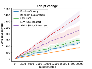
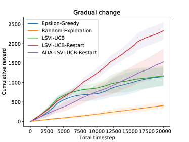
Figure 2: Comparisons of different methods on cumulative reward under two different environments. The results are averaged over 10 trials and the error bars show the standard deviations. The environment changes abruptly in the left subfigure, whereas the environment changes gradually in the right subfigure.

From empirical studies, we find that the restart strategy works better under abrupt changes than under gradual changes, since the gap between our algorithms and the baseline algorithms is larger in this setting. The reason is that the algorithms designed to explore in stationary MDPs are generally insensitive to abrupt change in the environment. For example, UCB-type exploration does not have incentive to take actions other than the one with the largest upper confidence bound of $Q$-value, and if it has collected sufficient number of samples, it very likely never explores the new optimal action thereby taking the former optimal action forever. On the other hand, in gradually-changing environment, LSVI-UCB and Epsilon-Greedy can perform well in the beginning when the drift of environment is small. However, when the change of environment is greater, they no longer yield satisfactory performance since their $Q$ function estimate is quite off. This also explains why LSVI-UCB and Epsilon-Greedy outperform ADA-LSVI-UCB at the beginning in the gradually-changing environment, as shown in Fig. 2.

Fig. 3 shows that the running times of LSVI-UCB-Restart and Ada-LSVI-UCB-Restart are roughly the same. They are much less compared with LSVI-UCB and Epsilon-Greedy. This is because LSVI-UCB-Restart and Ada-LSVI-UCB-Restart can automatically restart according to the variation of the environment and thus have much smaller length of the trajectory and computational burden. Although Random-Exploration takes the least time, it cannot find the near-optimal policy. This result further demonstrates that our algorithms are not only sample-efficient, but also computationally tractable.

Figure 3: Comparisons of different methods on running time for two different environments. The results are averaged over 10 trials and the error bars show the standard deviations. See Appendix E-B for details on hardware.

VII Conclusion and Future Work

In this paper, we studied nonstationary RL with time-varying reward and transition functions. We focused on the class of nonstationary linear MDPs such that linear function approximation is sufficient to realize any value function. We first incorporated the epoch start strategy into LSVI-UCB algorithm [1] to propose the LSVI-UCB-Restart algorithm with low dynamic regret when the total variations are known. We then designed a parameter-free algorithm Ada-LSVI-UCB-Restart that enjoys a slightly worse dynamic regret bound without knowing the total variations. We derived a minimax regret lower bound is for nonstationary linear MDPs to demonstrate that our proposed algorithms are near-optimal. Specifically, when the local variations are known, LSVI-UCB-Restart is near order-optimal except for the dependency on feature dimension $d$, planning horizon $H$, and some poly-logarithmic factors. Numerical experiments demonstrates the effectiveness of our algorithms.

A number of future directions are of interest. An immediate step is to investigate whether the dependence on the dimension $d$ and planning horizon $H$ in our bounds can be improved, and whether the minimax regret lower bound can also be improved. It would also be interesting to investigate the setting of nonstationary RL under general function approximation [14], which is closer to modern RL algorithms in practice.

Appendix A Proofs in Section III

In this section, we prove the minimax regret lower bound of nonstationary linear MDP. We first prove the regret lower bound of stationary linear MDP.

Proof of Theorem 1.

Let $\mathbb{P}^{\pi}_{t,\bm{v}}$ (assume $t$ is a multiple of $H$) be the probability distribution of
$\{a_{1}^{1},\sum_{h=1}^{H}r_{h}^{1},a_{1}^{2},\sum_{h=1}^{H}r_{h}^{2},\ldots,a_{1}^{t/H},\sum_{h=1}^{H}r_{h}^{t/H}\}$ of running algorithm $\pi$ on linear MDP parametrized by $\bm{v}$. First note that by the Markov property of $\pi$, we can decompose $D_{KL}(\mathbb{P}^{\pi}_{t,\bm{v}}||\mathbb{P}^{\pi}_{t,\bm{v}^{\prime}})$ as

$$\sum_{l=1}^{t/H}\mathbb{E}D_{KL}\left(\mathbb{P}\left(\sum_{h=1}^{H}r_{h}^{l}|a_{1}^{l},\bm{v}\right)||\mathbb{P}\left(\sum_{h=1}^{H}r_{h}^{l}|a_{1}^{l},\bm{v}^{\prime}\right)\right).$$

Recall that due to our hard cases construction, the first step in every episode determines the distribution of the total reward of that episode, thus

$$D_{KL}\left(\mathbb{P}\left(\sum_{h=1}^{H}r_{h}^{l}|a_{1}^{l},\bm{v}\right)||\mathbb{P}\left(\sum_{h=1}^{H}r_{h}^{l}|a_{1}^{l},\bm{v}^{\prime}\right)\right)$$

$$= \left(\delta+\langle\bm{a}_{1}^{l},\bm{v}\rangle\right)\log\frac{\delta+\langle\bm{a}_{1}^{l},\bm{v}\rangle}{\delta+\langle\bm{a}_{1}^{l},\bm{v}^{\prime}\rangle}+\left(1-\delta-\langle\bm{a}_{1}^{l},\bm{v}\rangle\right)\log\frac{1-\delta-\langle\bm{a}_{1}^{l},\bm{v}\rangle}{1-\delta-\langle\bm{a}_{1}^{l},\bm{v}^{\prime}\rangle}$$ (5)

We bound the KL divergence in (A) applying the following lemma.

Lemma 5.

[34] If $0\leq\delta^{\prime}\leq 1/2$ and $\epsilon^{\prime}\leq 1-2\delta^{\prime}$, then

$$\delta^{\prime}\log\frac{\delta^{\prime}}{\delta^{\prime}+\epsilon^{\prime}}+(1-\delta^{\prime})\log\frac{1-\delta^{\prime}}{1-\delta^{\prime}-\epsilon^{\prime}}\leq\frac{2(\epsilon^{\prime})^{2}}{\delta^{\prime}}.$$

To apply Lemma 5, we let $\langle\bm{a}_{1}^{l},\bm{v}\rangle+\delta=\delta^{\prime}$, $\langle\bm{v}-\bm{v}^{\prime},\bm{a}_{1}^{l}\rangle=\epsilon^{\prime}$. Thus we must ensure the following inequalities hold for any $\bm{a},\bm{v},\bm{v}^{\prime}$:

$$\langle\bm{a},\bm{v}\rangle+\delta \leq\frac{(d-3)\sqrt{H}}{\sqrt{T}}+\delta\leq 1/2$$

$$\langle\bm{v}-\bm{v}^{\prime},\bm{a}\rangle \leq\frac{2(d-3)\sqrt{H}}{\sqrt{T}}\leq 1-2\left(\frac{(d-3)\sqrt{H}}{\sqrt{T}}+\delta\right)\leq 1-2\delta^{\prime}.$$

To guarantee the above inequalities hold, we can set $\delta=\frac{1}{4}$ and let $\frac{(d-3)\sqrt{H}}{\sqrt{T}}\leq\frac{1}{8}$. Now we get back to bounding Eq. A. Let $\Delta=\frac{(d-3)\sqrt{H}}{\sqrt{T}}$ and suppose $\bm{v}$ and $\bm{v}^{\prime}$ only differ in one coordinate. Then

$$D_{KL}\left(\mathbb{P}\left(\sum_{h=1}^{H}r_{h}^{l}|a_{1}^{l},\bm{v}\right)||\mathbb{P}\left(\sum_{h=1}^{H}r_{h}^{l}|a_{1}^{l},\bm{v}^{\prime}\right)\right) \leq\frac{8\Delta^{2}\frac{1}{(d-3)^{2}}}{\delta-\Delta}\leq\frac{16\Delta^{2}}{\delta(d-3)^{2}}\leq\frac{64H}{T}.$$

Furthermore, let $E_{i,b}$ be the the following event:

$$|\{l\in[K]:\text{sgn}(\bm{a}_{1}^{l})_{i}\neq b\}|\geq\frac{1}{2}K.$$

In other words $E_{i,b}$ is the event that the learner take sup-optimal action for one coordinate for more than half of the episodes. Let $q_{i,\bm{v}}=\mathbb{P}[E_{i,v_{i}}|\bm{v}]$, the probability that the agent is taking sub-optimal action for the $i$-th coordinate for at least half of the episodes given that the underlying linear MDP is parameteriezed by $\bm{v}$. We can then lower bound the regret of any algorithm when running on linear MDP parameterized by $\bm{v}$ as:

$$\text{Reg}_{\bm{v}}(T) \geq\sum_{i=1}^{d-3}q_{i,\bm{v}}\frac{1}{2}K(H-1)\sqrt{\frac{H}{T}}$$

$$\geq\left(\sqrt{TH}-\sqrt{\frac{H^{2}}{T}}\right)\sum_{i=1}^{d-3}q_{i,\bm{v}},$$ (6)

since whenever the learner takes a sub-optimal action that differs from the optimal action by one coordinate, it will incur $2\sqrt{\frac{H}{T}}(H-1)$ expected regret. Next we take the average over $2^{d-3}$ linear MDP instances to show that on average it incurs $\Omega(d\sqrt{HT})$ regret, thus there exists at least one instance incurring $\Omega(d\sqrt{HT})$ regret. Before that, we need to bound the summation of bad events under two close linear MDP instances. Denote the vector which is only different from $\bm{v}$ in $i$-th coordinate as $\bm{v}^{\oplus i}$. Then we have

$$q_{i,\bm{v}}+q_{i,\bm{v}^{\oplus i}} =\mathbb{P}[E_{i,\bm{v}_{i}}|\bm{v}]+\mathbb{P}[E_{i,\bm{v}^{\oplus i}_{i}}|\bm{v}^{\oplus i}]$$

$$=\mathbb{P}[E_{i,\bm{v}_{i}}|\bm{v}]+\mathbb{P}[\bar{E}_{i,\bm{v}_{i}}|\bm{v}^{\oplus i}]$$

$$\geq\tfrac{1}{2}\exp(-D_{KL}(P_{T,\bm{v}}||P_{T,\bm{v}^{\oplus i}}))$$

$$\geq\tfrac{1}{2}\exp(-64),$$ (7)

where the inequality is due to Bretagnolle-Huber inequality [52]. Now we are ready to lower bound the average regret over all linear MDP instances.

$$\frac{1}{2^{d-3}}\sum_{\bm{v}}\text{Reg}_{\bm{v}}(T) \geq\frac{\sqrt{HT}-\sqrt{\frac{H^{2}}{T}}}{2^{d-3}}\sum_{\bm{v}}\sum_{i=1}^{d-3}q_{i,\bm{v}}$$

$$\geq\frac{\sqrt{HT}-\sqrt{\frac{H^{2}}{T}}}{2^{d-3}}\sum_{i=1}^{d-3}\sum_{\bm{v}}\frac{q_{i,\bm{v}}+q_{i,\bm{v}^{\oplus i}}}{2}$$

$$\geq\frac{\sqrt{HT}-\sqrt{\frac{H^{2}}{T}}}{2^{d-3}}2^{d-3}\frac{1}{4}e^{-64}(d-3)$$

$$\gtrsim\Omega(d\sqrt{HT})$$

where the first inequality is due to (A), and the third inequality is due to (A). ∎

Based on Thm. 1, we can derive the minimax dynamic regret for nonstationary linear MDP.

Proof of Thm. 2.

We construct the hard instance as follows: We first divide the whole time horizon $T$ into $\lceil\frac{K}{N}\rceil$ intervals, where each interval has $\lceil\frac{K}{N}\rceil$ episodes (the last interval might be shorter if $K$ is not a multiple of $N$). For each interval, the linear MDP is fixed and parameterized by a $\bm{v}\in\{\pm\frac{\sqrt{(d-3)}}{\sqrt{N}}\}^{d-3}$ which we define when constructing the hard instances in Thm. 1. Note that different intervals are completely decoupled, thus information is not passed across intervals. For each interval, it incurs regret at least $\Omega(d\sqrt{H^{2}N})$ by Thm. 1. Thus the total regret is at least

$$\text{Dyn-Reg}(T) \gtrsim(\lceil\frac{K}{N}\rceil-1)\Omega(d\sqrt{H^{2}N})$$

$$\gtrsim\Omega(d\sqrt{H^{2}K^{2}}N^{-1/2}).$$ (8)

Intuitively, we would like $N$ to be as small as possible to obtain a tight lower bound. However, due to our construction, the total variation for two consecutive blocks is upper-bounded by

$$\sqrt{\sum_{i=1}^{d-3}\frac{4(d-3)}{N}}=\frac{2(d-3)}{\sqrt{N}}\mbox{.}$$

Note that the total time variation for the whole time horizon is $B$ and by definition $B\geq\frac{2(d-3)}{\sqrt{N}}(\lfloor\frac{K}{N}\rfloor-1)$, which implies$N\gtrsim\Omega(B^{-2/3}d^{2/3}K^{2/3})$. Substituting the lower bound of $N$ into (A), we have

$$\text{Dyn-Reg}(T)\gtrsim\Omega(B^{1/3}d^{2/3}K^{2/3}H)\gtrsim\Omega(B^{1/3}d^{2/3}H^{1/3}T^{2/3})$$

which concludes the proof. ∎

Next we prove the dynamic regret lower bound for infinite-horizon average-reward tabular MDP. Similar to prove the regret lower bound for nonstationary linear MDP, the lower bound construction for nonstationary tabular MDP is based on concatenating lower bound constructinon for stationary tabular MDP with different optimal policies.

Proof of Corollary 1.

From [34], we know for the stationary case, the minimax regret lower bound for stationary infinite-horizon average-reward tabular MDP is $\Omega{\sqrt{D_{\max}SAT}}$. Note that in their lower bound construction, the reward function is a deterministic function of the states (for the detailed construction, please refer to [34]), and there is only one optimal action $a^{*}$ that can maximize the reaching probability to the states with positive reward. Thus by changing $a^{*}$, we can construct a nonstaionary MDP instance with $B_{r}=0$ and $B_{p}>0$ (note that changing $a^{*}$ does not change the diameter of the MDP). The construction is detailed as follows, first partition the whole time horizon $T$ into blocks of equal length $W$ (the last block might be shorter). Thus the dynamic regret is lower bounded by

$$\text{Dyn-Reg}(T) \gtrsim\Omega(\sqrt{D_{\max}SAW})(\lceil\frac{T}{W}\rceil-1)$$

$$\gtrsim\Omega(D_{\max}^{1/2}S^{1/2}A^{1/2}TW^{-1/2}).$$ (9)

From [34], we know the optimal action $a^{*}$ can transition to the state with positive reward with higher probability, and the gap compared to other actions is $\Theta(\sqrt{\frac{SA}{WD}})$. Thus the total variation in transition function is $B=B_{p}=\Theta(D^{-1/2}S^{1/2}A^{1/2}W^{-3/2}T)$, so the length of each block is $W=\Theta(B^{-2/3}D^{-1/3}S^{1/3}A^{1/3}T^{2/3})$. Substituting the block size $W$ into (A), we have the dynamic regret lower bound is $\Omega(D^{2/3}B^{1/3}S^{1/3}A^{1/3}T^{2/3})$. ∎

Appendix B Proofs in Section IV

Here we provide the proofs in Sec. IV. First, we introduce some notations we use throughout the proof. We let $\bm{w}^{k}_{h}$, $\Lambda^{k}_{h}$ and $Q^{k}_{h}$ as the parameters and action-value function estimate in episode $k$ for step $h$. Denote value function estimate as $V^{k}_{h}(s)=\max_{a}Q^{k}_{h}(s,a)$. For any policy $\pi$, we let $\bm{w}^{\pi}_{h,k}$, $Q^{\pi}_{h,k}$ be the ground-truth parameter and action-value function for that policy in episode $k$ for step $h$. We also abbreviate $\bm{\phi}(s_{h}^{l},a_{h}^{l})$ as $\bm{\phi}_{h}^{l}$ for notational simplicity.

We first work on the case when local variation is known and then consider the case when local variation is unknown.

B-A Case 1: Known Local Variation

Before we prove the regret upper bound within one epoch (Thm. 5), we need some additional lemmas.
The first lemma is used to control the fluctuations in least-squares value iteration, when performed on the value function estimate $V_{h}^{k}(\cdot)$ maintained in Alg. 1.

Proof of Lemma 1.

The lemma is slightly different than [1, Lemma B.3], since they assume $\mathbb{P}_{h}$ is fixed for different episodes. It can be verified that the proof for stationary case still holds in our case without any modifications since the results in [1] holds for least-squares value iteration for arbitrary function in the function class of our interest, i.e., $\{V|V=\{\bm{\phi}(\cdot,\cdot),\bm{w}\},\bm{w}\in\mathbb{R}^{d}\}$. ∎

We then proceed to derive the error bound for the action-value function estimate maintained in the algorithm for any policy.

Proof of Lemma 2.

Note that $Q^{\pi}_{h,k}(s,a)=\langle\phi(s,a),\bm{w}^{\pi}_{h,k}\rangle$. First we can decompose $\bm{w}_{h}^{k}-\bm{w}^{\pi}_{h,k}$ as

$$\bm{w}_{h}^{k}-\bm{w}^{\pi}_{h,k} =(\Lambda^{k}_{h})^{-1}\sum_{l=\tau}^{k-1}\bm{\phi}^{l}_{h}[r^{l}_{h}(s^{l}_{h},a^{l}_{h})+V_{h+1}^{k}(s_{h+1}^{l})]-\bm{w}^{\pi}_{h,k}$$

$$=(\Lambda^{k}_{h})^{-1}\{-\bm{w}^{\pi}_{h,k}+\sum_{l=\tau}^{k-1}\bm{\phi}^{l}_{h}[V^{k}_{h+1}(s^{l}_{h+1})-\mathbb{P}_{h}^{k}V^{\pi}_{h+1,k}(s^{l}_{h},a^{l}_{h})]+\sum_{l=\tau}^{k-1}\bm{\phi}_{h}^{l}[r_{h}^{l}(s_{h}^{l},a_{h}^{l})-r_{h}^{k}(s_{h}^{l},a_{h}^{l})]\}$$

$$=\underbrace{-(\Lambda^{k}_{h})^{-1}\bm{w}^{\pi}_{h,k}}_{\leavevmode\hbox to8.08pt{\vbox to8.08pt{\text{[drawing]}}}}+\underbrace{(\Lambda_{h}^{k})^{-1}\sum_{l=\tau}^{k-1}\bm{\phi}_{h}^{l}[V^{k}_{h+1}(s_{h+1}^{l})-\mathbb{P}_{h}^{l}V^{k}_{h+1}(s_{h}^{l},a_{h}^{l})]}_{\leavevmode\hbox to8.08pt{\vbox to8.08pt{\text{[drawing]}}}}$$

$$\quad+\underbrace{(\Lambda_{h}^{k})^{-1}\sum_{l=\tau}^{k-1}\bm{\phi}_{h}^{l}[(\mathbb{P}_{h}^{l}-\mathbb{P}_{h}^{k})V^{k}_{h+1}(s_{h}^{l},a_{h}^{l})]}_{\leavevmode\hbox to8.08pt{\vbox to8.08pt{\text{[drawing]}}}}+\underbrace{(\Lambda^{k}_{h})^{-1}\sum_{l=\tau}^{k-1}\bm{\phi}_{h}^{l}\mathbb{P}_{h}^{k}(V^{k}_{h+1}-V^{\pi}_{h+1,k})(s^{l}_{h},a^{l}_{h})}_{\leavevmode\hbox to8.08pt{\vbox to8.08pt{\text{[drawing]}}}}$$

$$\quad+\underbrace{(\Lambda^{k}_{h})^{-1}\sum_{l=\tau}^{k-1}\bm{\phi}_{h}^{l}[r_{h}^{l}(s_{h}^{l},a_{h}^{l})-r_{h}^{k}(s_{h}^{l},a_{h}^{l})]}_{\leavevmode\hbox to8.08pt{\vbox to8.08pt{\text{[drawing]}}}}.$$

We bound the individual terms on right side one by one. For the first term,

$$|\langle\bm{\phi}(s,a),\leavevmode\hbox to10.49pt{\vbox to10.49pt{\text{[drawing]}}}\rangle| =|\langle\bm{\phi}(s,a),(\Lambda^{k}_{h})^{-1}\bm{w}^{\pi}_{h,k}\rangle|$$

$$\leq\left\lVert\bm{w}^{\pi}_{h,k}\right\rVert\left\lVert\bm{\phi}(s,a)\right\rVert_{(\Lambda^{k}_{h})^{-1}}$$

$$\leq 2H\sqrt{d}\left\lVert\bm{\phi}(s,a)\right\rVert_{(\Lambda^{k}_{h})^{-1}},$$

where the last inequality is due to Lemma 9. For the second term, we know that under event $E$ defined in Lemma 1,

$$|\langle\bm{\phi}(s,a),\leavevmode\hbox to10.49pt{\vbox to10.49pt{\text{[drawing]}}}\rangle|\leq CdH\sqrt{\log[2(c_{\beta}+1)dW/p]}\left\lVert\bm{\phi}(s,a)\right\rVert_{(\Lambda^{k}_{h})^{-1}}.$$

For the third term,

$$\langle\bm{\phi}(s,a),\leavevmode\hbox to10.49pt{\vbox to10.49pt{\text{[drawing]}}}\rangle= \langle\bm{\phi}(s,a),(\Lambda_{h}^{k})^{-1}\sum_{l=\tau}^{k-1}\bm{\phi}_{h}^{l}[(\mathbb{P}_{h}^{l}-\mathbb{P}_{h}^{k})V^{k}_{h+1}(s_{h}^{l},a_{h}^{l})]\rangle$$

$$\leq \sum_{l=\tau}^{k-1}|\bm{\phi}(s,a)^{\top}(\Lambda^{k}_{h})^{-1}\bm{\phi}_{h}^{l}|[(\mathbb{P}_{h}^{l}-\mathbb{P}^{k}_{h})V_{h+1}^{k}(s^{l}_{h},a^{l}_{h})]$$

$$\leq B_{\bm{\mu},\mathcal{E}}H\sum_{l=\tau}^{k-1}|\bm{\phi}(s,a)^{\top}(\Lambda^{k}_{h})^{-1}\bm{\phi}_{h}^{l}|$$

$$\leq B_{\bm{\mu},\mathcal{E}}H\sqrt{\sum_{l=\tau}^{k-1}\left\lVert\bm{\phi}(s,a)\right\rVert_{(\Lambda_{h}^{k})^{-1}}}\sqrt{\sum_{l=\tau}^{k-1}(\bm{\phi}_{h}^{l})^{\top}(\Lambda_{h}^{k})^{-1}\bm{\phi}_{h}^{l}}$$

$$\leq \sqrt{d(k-\tau)}B_{\bm{\mu},\mathcal{E}}H\left\lVert\bm{\phi}(s,a)\right\rVert_{(\Lambda_{h}^{k})^{-1}},$$

where the first three inequalities are due to Cauchy-Schwarz inequality and boundedness of $\mathbb{P}_{h}^{l}-\mathbb{P}_{h}^{k}$ and $V^{k}_{h+1}$, and the last inequality is due to Lemma 10.

For the fourth term,

$$\langle\bm{\phi}(s,a),\leavevmode\hbox to10.49pt{\vbox to10.49pt{\text{[drawing]}}}\rangle =\langle\bm{\phi}(s,a),(\Lambda^{k}_{h})^{-1}\sum_{l=\tau}^{k-1}\bm{\phi}_{h}^{l}\mathbb{P}_{h}^{k}(V^{k}_{h+1}-V^{\pi}_{h+1,k})(s^{l}_{h},a^{l}_{h})\rangle$$

$$=\langle\bm{\phi}(s,a),(\Lambda^{k}_{h})^{-1}\sum_{l=\tau}^{k-1}\bm{\phi}_{h}^{l}(\bm{\phi}_{h}^{l})^{\top}\int(V_{h+1}^{k}(s^{\prime})-V^{\pi}_{h+1,k}(s^{\prime}))d\bm{\mu}_{h,k}(s^{\prime})\rangle$$

$$=\underbrace{\langle\bm{\phi}(s,a),\int(V^{k}_{h+1}-V^{\pi}_{h+1,k})(s^{\prime})d\bm{\mu}_{h,k}(s^{\prime})\rangle}_{\leavevmode\hbox to8.08pt{\vbox to8.08pt{\text{[drawing]}}}}\rangle-\underbrace{\langle\bm{\phi}(s,a),(\Lambda^{k}_{h})^{-1}\int(V^{k}_{h+1}-V^{\pi}_{h+1,k})(s^{\prime})d\bm{\mu}_{h,k}(s^{\prime})\rangle}_{\leavevmode\hbox to8.08pt{\vbox to8.08pt{\text{[drawing]}}}},$$

where $\leavevmode\hbox to10.49pt{\vbox to10.49pt{\text{[drawing]}}}=[\mathbb{P}_{h}^{k}(V^{k}_{h+1}-V^{\pi}_{h+1,k})](s,a)$ and $\leavevmode\hbox to10.49pt{\vbox to10.49pt{\text{[drawing]}}}\leq 2H\sqrt{d}\left\lVert\bm{\phi}(s,a)\right\rVert_{(\Lambda^{k}_{h})^{-1}}$ due to Cauchy-Schwarz inequality.

For the fifth term,

$$\langle\bm{\phi}(s,a),\leavevmode\hbox to10.49pt{\vbox to10.49pt{\text{[drawing]}}}\rangle =\langle\bm{\phi}(s,a),(\Lambda^{k}_{h})^{-1}\sum_{l=\tau}^{k-1}\bm{\phi}_{h}^{l}[r_{h}^{l}(s_{h}^{l},a_{h}^{l})-r_{h}^{k}(s_{h}^{l},a_{h}^{l})]\rangle$$

$$\leq\sum_{l=\tau}^{k-1}|\bm{\phi}(s,a)^{\top}(\Lambda_{h}^{k})^{-1}\bm{\phi}^{l}_{h}||r^{l}_{h}(s_{h}^{l},a_{h}^{l})-r^{k}_{h}(s_{h}^{l},a_{h}^{l})|$$

$$\leq\sqrt{d(k-\tau)}B_{\bm{\theta},\mathcal{E}}\left\lVert\bm{\phi}(s,a)\right\rVert_{(\Lambda^{k}_{h})^{-1}},$$

where the inequalities are derived similarly as bounding the third term. After combining all the upper bounds for these individual terms, we have

$$|\langle\bm{\phi}(s,a),\bm{w}_{h}^{k}\rangle-Q^{\pi}_{h,k}(s,a)-\mathbb{P}_{h}^{k}\left(V^{k}_{h+1}-V^{\pi}_{h+1,k}\right)(s,a)|$$

$$\leq 4H\sqrt{d}\left\lVert\bm{\phi}(s,a)\right\rVert_{(\Lambda^{k}_{h})^{-1}}+CdH\sqrt{\log[2(c_{\beta}+1)dW/p]}\left\lVert\bm{\phi}(s,a)\right\rVert_{(\Lambda^{k}_{h})^{-1}}$$

$$\quad+B_{\bm{\theta},\mathcal{E}}\sqrt{d(k-\tau)}\left\lVert\bm{\phi}(s,a)\right\rVert_{(\Lambda^{k}_{h})^{-1}}+B_{\bm{\mu},\mathcal{E}}H\sqrt{d(k-\tau)}\left\lVert\bm{\phi}(s,a)\right\rVert_{(\Lambda^{k}_{h})^{-1}}$$

$$\leq C_{0}dH\sqrt{\log[2dW/p]}\left\lVert\bm{\phi}(s,a)\right\rVert_{(\Lambda^{k}_{h})^{-1}}+B_{\bm{\theta},\mathcal{E}}\sqrt{d(k-\tau)}\left\lVert\bm{\phi}(s,a)\right\rVert_{(\Lambda^{k}_{h})^{-1}}$$

$$\quad+B_{\bm{\mu},\mathcal{E}}H\sqrt{d(k-\tau)}\left\lVert\bm{\phi}(s,a)\right\rVert_{(\Lambda^{k}_{h})^{-1}}.$$

The second inequality holds if we choose a sufficiently large absolute constant $C_{0}$. ∎

Lemma 2 implies that the action-value function estimate we maintained in Alg. 1 is always an optimistic upper bound of the optimal action-value function with high confidence, if we know the local variation.

Proof of Lemma 3.

We prove this by induction. First prove the base case when $h=H$. According to Lemma 2, we have

$$|\langle\bm{\phi}(s,a),\bm{w}^{k}_{H}\rangle-Q^{*}_{H,k}(s,a)|\leq\beta_{k}\left\lVert\bm{\phi}(s,a)\right\rVert_{(\Lambda^{k}_{H})^{-1}},$$

which implies

$$Q_{H}^{k}(s,a) =\min\{\langle\bm{w}^{k}_{H},\bm{\phi}(s,a)\rangle+\beta_{k}\left\lVert\bm{\phi}(s,a)\right\rVert_{(\Lambda^{k}_{H})^{-1}},H\}\geq Q^{*}_{H,k}(s,a).$$

Now suppose the statement holds true at step $h+1$, then for step $h$, due to Lemma 2, we have

$$|\langle\bm{\phi}(s,a),\bm{w}_{h}^{k}\rangle-Q^{\pi}_{h,k}(s,a)-\mathbb{P}_{h}^{k}(V^{k}_{h+1}-V^{*}_{h+1,k})(s,a)|\leq\beta_{k}\left\lVert\bm{\phi}(s,a)\right\rVert_{(\Lambda^{k}_{h})^{-1}}.$$

By the induction hypothesis, we have $\mathbb{P}_{h}^{k}(V^{k}_{h+1}-V^{*}_{h+1,k})(s,a)\geq 0$, thus

$$Q_{h}^{k}(s,a) =\min\{\langle\bm{w}^{k}_{h},\bm{\phi}(s,a)\rangle+\beta_{k}\left\lVert\bm{\phi}(s,a)\right\rVert_{(\Lambda^{k}_{H})^{-1}},H\}\geq Q^{*}_{h,k}(s,a).$$

∎

Next we derive the bound for the gap between the value function estimate and the ground-truth value function for the executing policy $\pi^{k}$, $\delta^{k}_{h}=V^{k}_{h}(s^{k}_{h})-V^{\pi^{k}}_{h,k}(s^{k}_{h})$, in a recursive manner.

Lemma 6.

Let $\delta^{k}_{h}=V^{k}_{h}(s^{k}_{h})-V^{\pi^{k}}_{h,k}(s^{k}_{h})$, $\zeta^{k}_{h+1}=\mathbb{E}[\delta^{k}_{h+1}|s^{k}_{h},a^{k}_{h}]-\delta^{k}_{h+1}$. Under event $E$ defined in Lemma 1, we have for all $(k,h)\in\mathcal{E}\times[H]$,

$$\delta_{h}^{k}\leq\delta^{k}_{h+1}+\zeta_{h+1}^{k}+2\beta_{k}\left\lVert\bm{\phi}_{h}^{k}\right\rVert_{(\Lambda^{k}_{h})^{-1}}.$$

Proof.

By Lemma 2, for any $(s,a,h,k)\in\mathcal{S}\times\mathcal{A}\times[H]\times\mathcal{E}$,

$$Q_{h}^{k}(s,a)-Q_{h}^{\pi^{k}}(s,a) \leq\mathbb{P}_{h}^{k}(V^{k}_{h+1}-V^{\pi^{k}}_{h+1,k})(s,a)+2\beta_{k}\left\lVert\bm{\phi}(s,a)\right\rVert_{(\Lambda^{k}_{H})^{-1}}.$$

Note that $Q_{h}^{k}(s_{h}^{k},a_{h}^{k})=\max_{a}Q_{h}^{k}(s_{h}^{k},a)=V_{h}^{k}(s_{h}^{k})$ according to Algorithm 1, and $Q_{h,k}^{\pi^{k}}(s_{h}^{k},a_{h}^{k})=V^{\pi^{k}}_{h,k}(s_{h}^{k})$ by the definition. Thus,

$$\delta_{h}^{k}\leq\delta^{k}_{h+1}+\zeta_{h+1}^{k}+2\beta_{k}\left\lVert\bm{\phi}_{h}^{k}\right\rVert_{(\Lambda^{k}_{h})^{-1}}.$$

∎

Now we are ready to derive the regret bound within one epoch.

Proof of Theorem 3.

We denote the dynamic regret within that epoch as $\text{Dyn-Reg}(\mathcal{E})$. We define $\delta^{k}_{h}=V^{k}_{h}(s^{k}_{h})-V^{\pi^{k}}_{h,k}(s^{k}_{h})$ and $\zeta^{k}_{h+1}=\mathbb{E}[\delta^{k}_{h+1}|s^{k}_{h},a^{k}_{h}]-\delta^{k}_{h+1}$ as in Lemma 8. We derive the dynamic regret within a epoch $\mathcal{E}$ (the length of this epoch is $W$ which is equivalent to $\frac{W}{H}$ episodes) conditioned on the event $E$ defined in Lemma 1 which happens with probability at least $1-p/2$.

$$\text{Dyn-Reg}(\mathcal{E}) =\sum_{k\in\mathcal{E}}\left[V^{*}_{1,k}(s^{k}_{1})-V^{\pi^{k}}_{1,k}\right]$$

$$\leq\sum_{k\in\mathcal{E}}\left[V^{k}_{1}(s^{k}_{1})-V^{\pi^{k}}_{1,k}\right]$$

$$\leq\sum_{k\in\mathcal{E}}\delta^{k}_{1}$$

$$\leq\sum_{k\in\mathcal{E}}\sum_{h=1}^{H}\zeta^{k}_{h}+2\sum_{k\in\mathcal{K}}\beta_{k}\sum_{h=1}^{H}\left\lVert\bm{\phi}^{k}_{h}\right\rVert_{(\Lambda^{k}_{h})^{-1}},$$ (10)

where the first inequality is due to Lemma 3, the third inequality is due to Lemma 6. For the first term in the right side, since $V_{h}^{k}$ is independent of the new observation $s_{h}^{k}$, $\{\zeta_{h}^{k}\}$ is a martingale difference sequence. Applying the Azuma-Hoeffding inequlity, we have for any $t>0$,

$$\mathbb{P}\left(\sum_{k\in\mathcal{E}}\sum_{h=1}^{H}\zeta_{h}^{k}\geq t\right)\geq\exp(-t^{2}/(2WH^{2})).$$

Hence with probability at least $1-p/2$, we have

$$\sum_{k\in\mathcal{E}}\sum_{h=1}^{H}\zeta_{h}^{k}\leq 2H\sqrt{W\log(2dW/p)}.$$ (11)

For the second term, we bound via Cauchy-Schwarz inequality:

$$2\sum_{k\in\mathcal{E}}\beta_{k}\sum_{h=1}^{H}\left\lVert\bm{\phi}^{k}_{h}\right\rVert_{(\Lambda^{k}_{h})^{-1}} =2C_{0}dH\sqrt{\log 2(dW/p)}\sum_{k\in\mathcal{E}}\sum_{h=1}^{H}\left\lVert\bm{\phi}_{h}^{k}\right\rVert_{(\Lambda_{h}^{k})^{-1}}+2\sum_{k\in\mathcal{E}}B_{\theta,\mathcal{E}}\sqrt{d(k-\tau)}\sum_{h=1}^{H}\left\lVert\bm{\phi}_{h}^{k}\right\rVert_{(\Lambda_{h}^{k})^{-1}}$$

$$\quad+2\sum_{k\in\mathcal{E}}B_{\bm{\mu}}H\sqrt{d(k-\tau)}\sum_{h=1}^{H}\left\lVert\bm{\phi}_{h}^{k}\right\rVert_{(\Lambda_{h}^{k})^{-1}}$$

$$\leq 2C_{0}dH\sqrt{\log 2(dW/p)}\sum_{h=1}^{H}\sqrt{W/H}(\sum_{k\in\mathcal{E}}\left\lVert\bm{\phi}_{h}^{k}\right\rVert^{2}_{(\Lambda_{h}^{k})^{-1}})^{1/2}$$

$$\quad+2\sum_{h=1}^{H}(\sum_{k\in\mathcal{E}}B_{\bm{\theta},\mathcal{E}}\sqrt{d(k-\tau)})^{1/2}(\sum_{k\in\mathcal{E}}\left\lVert\bm{\phi}_{h}^{k}\right\rVert^{2}_{(\Lambda_{h}^{k})^{-1}})^{1/2}$$

$$\quad+2\sum_{h=1}^{H}(\sum_{k\in\mathcal{E}}B_{\bm{\mu},\mathcal{E}}H\sqrt{d(k-\tau)})^{1/2}(\sum_{k\in\mathcal{E}}\left\lVert\bm{\phi}_{h}^{k}\right\rVert^{2}_{(\Lambda_{h}^{k})^{-1}})^{1/2}$$

$$\leq 2C_{0}dH\sqrt{\log 2(dW/p)}\sum_{h=1}^{H}\sqrt{W/H}(\sum_{k\in\mathcal{E}}\left\lVert\bm{\phi}_{h}^{k}\right\rVert^{2}_{(\Lambda_{h}^{k})^{-1}})^{1/2}$$

$$\quad+2\sum_{h=1}^{H}B_{\bm{\theta},\mathcal{E}}\sqrt{d}\frac{W}{H}(\sum_{k\in\mathcal{E}}\left\lVert\bm{\phi}_{h}^{k}\right\rVert^{2}_{(\Lambda_{h}^{k})^{-1}})^{1/2}$$

$$\quad+2\sum_{h=1}^{H}B_{\bm{\theta},\mathcal{E}}\sqrt{d}W(\sum_{k\in\mathcal{E}}\left\lVert\bm{\phi}_{h}^{k}\right\rVert^{2}_{(\Lambda_{h}^{k})^{-1}})^{1/2}$$ (12)

By Lemma 11, we have

$$(\sum_{k\in\mathcal{E}}\left\lVert\bm{\phi}_{h}^{k}\right\rVert^{2}_{(\Lambda_{h}^{k})^{-1}})^{1/2}\leq\sqrt{d\log\left(\frac{W}{H}+1\right)}.$$ (13)

Finally, by combining Eq. B-A–13, we obtain the regret bound within the epoch $\mathcal{E}$ as:

$$\text{Dyn-Reg}(\mathcal{E})\lesssim\tilde{O}(H^{3/2}d^{3/2}W^{1/2}+B_{\bm{\theta},\mathcal{E}}dW+B_{\bm{\mu},\mathcal{E}}dHW).$$

∎

By summing over all epochs and applying a union bound, we obtain the regret bound for the whole time horizon.

Theorem 8.

If we set $\beta=\beta_{k}=cdH\sqrt{\log(2dT/p)}+B_{\bm{\theta},\mathcal{E}}\sqrt{d(k-\tau)}+B_{\bm{\mu},\mathcal{E}}H\sqrt{d(k-\tau)}$, the dynamic regret of LSVI-UCB-Restart is $\tilde{O}(H^{3/2}d^{3/2}TW^{-1/2}+B_{\bm{\theta}}dW+B_{\bm{\mu}}dHW)$, with probability at least $1-p$.

Proof.

In total there are $N=\lceil\frac{T}{W}\rceil$ epochs. For each epoch $\mathcal{E}_{i}$ if we set $\delta=\frac{p}{N}$, then it will incur regret $\tilde{O}(d^{3/2}H^{3/2}W^{1/2}+B_{\bm{\theta},\mathcal{E}_{i}}dW+B_{\bm{\mu},\mathcal{E}_{i}}dHW)$ with probability at least $1-\frac{p}{N}$. By summing over all epochs and applying the union bound over them, we can obtain the regret upper bound for the whole time horizon. With probability at least $1-p$,

$$\text{Dyn-Reg}(T) =\sum_{\mathcal{E}_{i}}\text{Dyn-Reg}(\mathcal{E}_{i})$$

$$\lesssim\sum_{\mathcal{E}_{i}}\tilde{O}(d^{3/2}H^{3/2}W^{1/2}+B_{\bm{\theta},\mathcal{E}_{i}}dW+B_{\bm{\mu},\mathcal{E}_{i}}dHW)$$

$$\lesssim\tilde{O}(H^{3/2}d^{3/2}TW^{-1/2}+B_{\bm{\theta}}dW+B_{\bm{\mu}}dHW).$$

∎

B-B Case 2: Unknown Local Variation

Similar to the case of known local variation, we first derive the error bound for the action-value function estimate maintained in the algorithm for any policy, which is the following technical lemma.

Lemma 7.

Under event $E$ defined in Lemma 1, we have for any policy $\pi$, $\forall s,a,h,k\in\mathcal{S}\times\mathcal{A}\times[H]\times\mathcal{E}$,

$$|\langle\bm{\phi}(s,a),\bm{w}_{h}^{k}\rangle-Q^{\pi}_{h,k}(s,a)-\mathbb{P}_{h}^{k}(V^{k}_{h+1}-V^{\pi}_{h+1,k})(s,a)|\leq\beta\left\lVert\bm{\phi}(s,a)\right\rVert_{(\Lambda^{k}_{h})^{-1}}+B_{\bm{\theta},\mathcal{E}}\sqrt{d(k-\tau)}+B_{\bm{\mu},\mathcal{E}}H\sqrt{d(k-\tau)},$$

where $\beta=C_{0}dH\sqrt{\log(2dW/p)}$ and $\tau$ is the first episode in the current epoch.

Proof.

This lemma is a looser upper bound implied by Lemma 2. By Lemma 2, we have

$$|\langle\bm{\phi}(s,a),\bm{w}_{h}^{k}\rangle-Q^{\pi}_{h,k}(s,a)-\mathbb{P}_{h}^{k}(V^{k}_{h+1}-V^{\pi}_{h+1,k})(s,a)|$$

$$\leq C_{o}dH\sqrt{\log(2dW/p)}\left\lVert\bm{\phi}(s,a)\right\rVert_{(\Lambda^{k}_{h})^{-1}}+B_{\bm{\theta},\mathcal{E}}\sqrt{d(k-\tau)}\left\lVert\bm{\phi}(s,a)\right\rVert_{(\Lambda^{k}_{h})^{-1}}$$

$$\quad+B_{\bm{\mu},\mathcal{E}}H\sqrt{d(k-\tau)}\left\lVert\bm{\phi}(s,a)\right\rVert_{(\Lambda^{k}_{h})^{-1}}$$

$$\leq C_{o}dH\sqrt{\log(2dW/p)}\left\lVert\bm{\phi}(s,a)\right\rVert_{(\Lambda^{k}_{h})^{-1}}+B_{\bm{\theta},\mathcal{E}}\sqrt{d(k-\tau)}$$

$$\quad+B_{\bm{\mu},\mathcal{E}}H\sqrt{d(k-\tau)},$$

where the second inequality is due to $\left\lVert\bm{\phi}(s,a)\right\rVert\leq 1$ and $\lambda_{\min}(\Lambda^{k}_{h})\geq 1$, thus $\left\lVert\bm{\phi}(s,a)\right\rVert_{(\Lambda^{k}_{h})^{-1}}\leq 1$. ∎

Different from Lemma 3, when the local variation is unknown, the action-value function estimate we maintained in Algorithm 1 is no longer an optimistic upper bound of the optimal action-value function, but approximately up to some error proportional to the local variation.

Proof of Lemma 4.

We prove this by induction. First prove the base case when $h=H$. According to Lemma 7, we have

$$|\langle\bm{\phi}(s,a),\bm{w}^{k}_{H}\rangle-Q^{*}_{H,k}(s,a)| \leq\beta\left\lVert\bm{\phi}(s,a)\right\rVert_{(\Lambda^{k}_{H})^{-1}}+B_{\bm{\theta},\mathcal{E}}\sqrt{d(k-\tau)}+B_{\bm{\mu},\mathcal{E}}H\sqrt{d(k-\tau)},$$

which implies

$$Q_{H}^{k}(s,a) =\min\{\langle\bm{w}^{k}_{H},\bm{\phi}(s,a)\rangle+\beta\left\lVert\bm{\phi}(s,a)\right\rVert_{(\Lambda^{k}_{H})^{-1}},H\}$$

$$\geq Q^{*}_{H,k}(s,a)-(B_{\bm{\theta},\mathcal{E}}\sqrt{d(k-\tau)}+B_{\bm{\mu},\mathcal{E}}H\sqrt{d(k-\tau)}).$$

Now suppose the statement holds true at step $h+1$, then for step $h$, due to Lemma 7, we have

$$|\langle\bm{\phi}(s,a),\bm{w}_{h}^{k}\rangle-Q^{\pi}_{h,k}(s,a)-\mathbb{P}_{h}^{k}(V^{k}_{h+1}-V^{*}_{h+1,k})(s,a)|$$

$$\leq \beta\left\lVert\bm{\phi}(s,a)\right\rVert_{(\Lambda^{k}_{h})^{-1}}+B_{\bm{\theta},\mathcal{E}}\sqrt{d(k-\tau)}+B_{\bm{\mu},\mathcal{E}}H\sqrt{d(k-\tau)}.$$

By the induction hypothesis, we have $[\mathbb{P}_{h}^{k}(V^{k}_{h+1}-V^{*}_{h+1,k})](s,a)\geq-(H-h+2)(B_{\bm{\theta},\mathcal{E}}\sqrt{d(k-\tau)}+B_{\bm{\mu},\mathcal{E}}H\sqrt{d(k-\tau)})$, thus

$$Q_{h}^{k}(s,a) =\min\{\langle\bm{w}^{k}_{h},\bm{\phi}(s,a)\rangle+\beta\left\lVert\bm{\phi}(s,a)\right\rVert_{(\Lambda^{k}_{H})^{-1}},H\}$$

$$\geq Q^{*}_{h,k}(s,a)-(H-h+1)(B_{\bm{\theta},\mathcal{E}}\sqrt{d(k-\tau)}+B_{\bm{\mu},\mathcal{E}}H\sqrt{d(k-\tau)}).$$

∎

Similar to Lemma 6, next we derive the bound for the gap between the value function estimate and the ground-truth value function for the executing policy $\pi^{k}$, $\delta^{k}_{h}=V^{k}_{h}(s^{k}_{h})-V^{\pi^{k}}_{h,k}(s^{k}_{h})$, in a recursive manner, when the local variation is unknown.

Lemma 8.

Let $\delta^{k}_{h}=V^{k}_{h}(s^{k}_{h})-V^{\pi^{k}}_{h,k}(s^{k}_{h})$, $\zeta^{k}_{h+1}=\mathbb{E}[\delta^{k}_{h+1}|s^{k}_{h},a^{k}_{h}]-\delta^{k}_{h+1}$. Under event $E$ defined in Lemma 1, we have for all $(k,h)\in\mathcal{E}\times[H]$,

$$\delta_{h}^{k} \leq\delta^{k}_{h+1}+\zeta_{h+1}^{k}+2\beta\left\lVert\bm{\phi}_{h}^{k}\right\rVert_{(\Lambda^{k}_{h})^{-1}}+B_{\bm{\theta},\mathcal{E}}\sqrt{d(k-\tau)}+B_{\bm{\mu},\mathcal{E}}H\sqrt{d(k-\tau)}.$$

Proof.

By Lemma 7, for any $(s,a,h,k)\in\mathcal{S}\times\mathcal{A}\times[H]\times\mathcal{E}$,

$$Q_{h}^{k}(s,a)-Q_{h}^{\pi^{k}}(s,a) \leq\mathbb{P}_{h}^{k}(V^{k}_{h+1}-V^{\pi^{k}}_{h+1,k})(s,a)+2\beta\left\lVert\bm{\phi}(s,a)\right\rVert_{(\Lambda^{k}_{H})^{-1}}+B_{\bm{\theta},\mathcal{E}}\sqrt{d(k-\tau)}+B_{\bm{\mu},\mathcal{E}}H\sqrt{d(k-\tau)}.$$

Note that $Q_{h}^{k}(s_{h}^{k},a_{h}^{k})=\max_{a}Q_{h}^{k}(s_{h}^{k},a)=V_{h}^{k}(s_{h}^{k})$ according to Algorithm 1, and $Q_{h,k}^{\pi^{k}}(s_{h}^{k},a_{h}^{k})=V^{\pi^{k}}_{h,k}(s_{h}^{k})$ by the definition. Thus,

$$\delta_{h}^{k} \leq\delta^{k}_{h+1}+\zeta_{h+1}^{k}+2\beta\left\lVert\bm{\phi}_{h}^{k}\right\rVert_{(\Lambda^{k}_{h})^{-1}}+B_{\bm{\theta},\mathcal{E}}\sqrt{d(k-\tau)}+B_{\bm{\mu},\mathcal{E}}H\sqrt{d(k-\tau)}.$$

∎

Now we are ready to prove Theorem 5, which is the regret upper bound within one epoch.

Proof of Theorem 5.

We denote the dynamic regret within an epoch as $\text{Dyn-Reg}(\mathcal{E})$. We define $\delta^{k}_{h}=V^{k}_{h}(s^{k}_{h})-V^{\pi^{k}}_{h,k}(s^{k}_{h})$ and $\zeta^{k}_{h+1}=\mathbb{E}[\delta^{k}_{h+1}|s^{k}_{h},a^{k}_{h}]-\delta^{k}_{h+1}$ as in Lemma 8. We derive the dynamic regret within a epoch $\mathcal{E}$ (the length of this epoch is $W$ which is equivalent to $\frac{W}{H}$ episodes) conditioned on the event $E$ defined in Lemma 1 which happens with probability at least $1-p/2$.

$$\text{Dyn-Reg}(\mathcal{E})$$

$$= \sum_{k\in\mathcal{E}}\left[V^{*}_{1,k}(s^{k}_{1})-V^{\pi^{k}}_{1,k}(s_{1}^{k})\right]$$

$$\leq \sum_{k\in\mathcal{E}}[V_{1}^{k}(s^{k}_{1})+B_{\bm{\theta},\mathcal{E}}H\sqrt{d(k-\tau)}+B_{\bm{\mu},\mathcal{E}}H^{2}\sqrt{d(k-\tau)}-V^{\pi^{k}}_{1,k}(s_{1}^{k})]$$

$$\leq \sum_{k\in\mathcal{E}}[\delta_{1}^{k}+B_{\bm{\theta},\mathcal{E}}H\sqrt{d(k-\tau)}+B_{\bm{\mu},\mathcal{E}}H^{2}\sqrt{d(k-\tau)}]$$

$$\leq \sum_{k\in\mathcal{E}}\sum_{h=1}^{H}\zeta_{h}^{k}+2\beta\sum_{k\in\mathcal{E}}\sum_{h=1}^{H}\left\lVert\bm{\phi}_{h}^{k}\right\rVert_{(\Lambda^{k}_{h})^{-1}}+2\sum_{k\in\mathcal{E}}B_{\bm{\theta},\mathcal{E}}H\sqrt{d(k-\tau)}+2\sum_{k\in\mathcal{E}}B_{\bm{\mu},\mathcal{E}}H^{2}\sqrt{d(k-\tau)}$$

$$\leq \sum_{k\in\mathcal{E}}\sum_{h=1}^{H}\zeta_{h}^{k}+2\beta\sum_{k\in\mathcal{E}}\sum_{h=1}^{H}\left\lVert\bm{\phi}_{h}^{k}\right\rVert_{(\Lambda^{k}_{h})^{-1}}+B_{\bm{\theta},\mathcal{E}}W\sqrt{2d(W/H+1)}+B_{\bm{\mu},\mathcal{E}}W\sqrt{2d(WH+H)}$$ (14)

where the first inequality is due to Lemma 4, the third inequality is due to Lemma 8, and the last inequality is due to Jensen’s inequality. Now we need to bound the first two terms in the right side. Note that $\{\zeta_{h}^{k}\}$ is a martingale difference sequence satisfying $|\zeta_{h}^{k}|\leq 2H$ for all $(k,h)$. By Azuma-Hoeffding inequality we have for any $t>0$,

$$\mathbb{P}\left(\sum_{k\in\mathcal{E}}\sum_{h=1}^{H}\zeta_{h}^{k}\geq t\right)\geq\exp(-t^{2}/(2WH^{2})).$$

Hence with probability at least $1-p/2$, we have

$$\sum_{k\in\mathcal{E}}\sum_{h=1}^{H}\zeta_{h}^{k}\leq 2H\sqrt{W\log(2dW/p)}.$$ (15)

For the second term, note that by Lemma 11 for any $h\in[H]$, we have

$$\sum_{k\in\mathcal{E}}(\bm{\phi}_{h}^{k})^{\top}(\Lambda^{k}_{h})^{-1}\bm{\phi}^{k}_{h} \leq 2\log\left[\frac{\det(\Lambda_{h}^{k+1})}{\det(\Lambda_{h}^{1})}\right]\leq 2d\log\left(\frac{W}{H}+1\right).$$

By Cauchy-Schwarz inequality, we have

$$\sum_{k\in\mathcal{E}}\sum_{h=1}^{H}\left\lVert\bm{\phi}_{h}^{k}\right\rVert_{(\Lambda^{k}_{h})^{-1}} \leq\sum_{h=1}^{H}\sqrt{W/H}\left[\sum_{k\in\mathcal{E}}(\bm{\phi}^{k}_{h})^{\top}(\Lambda^{k}_{h})^{-1}\bm{\phi}^{k}_{h}\right]^{1/2}$$

$$\leq H\sqrt{2d\frac{W}{H}\log\left(\frac{W}{H}+1\right)}$$

$$\leq H\sqrt{2d\frac{W}{H}\log\left[2dW/p\right]}.$$ (16)

Finally, combining (B-B)–(B-B), we have with probability at least $1-p$,

$$\text{Dyn-Reg}(\mathcal{E}) \leq 2H\sqrt{W\log(2dW/p)}+C_{0}dH^{2}\sqrt{\log(2dW)/p}\sqrt{2d\frac{W}{H}\log[2dW/p]}$$

$$\quad+B_{\bm{\theta},\mathcal{E}}W\sqrt{2d(W/H+1)}+B_{\bm{\mu},\mathcal{E}}W\sqrt{2d(WH+H)}$$

$$\lesssim\tilde{O}(\sqrt{d^{3}H^{3}W}+B_{\bm{\theta},\mathcal{E}}\sqrt{d/H}W^{3/2}+B_{\bm{\mu},\mathcal{E}}\sqrt{dH}W^{3/2}).$$

∎

Now we can derive the regret bound for the whole time horizon by summing over all epochs and applying a union bound. We restate the regret upper bound and provide its detailed proof.

Theorem 9.

If we set $\beta=cdH\sqrt{\log(2dT/p)}$, the dynamic regret of LSVI-UCB-Restart algorithm is $\tilde{O}(W^{-1/2}Td^{3/2}H^{3/2}+B_{\bm{\theta}}d^{1/2}H^{-1/2}W^{3/2}+B_{\bm{\mu}}d^{1/2}H^{1/2}W^{3/2})$, with probability at least $1-p$.

Proof.

In total there are $N=\lceil\frac{T}{W}\rceil$ epochs. For each epoch $\mathcal{E}_{i}$ if we set $\delta=\frac{p}{N}$, then it will incur regret $\tilde{O}(\sqrt{d^{3}H^{3}W}+B_{\bm{\theta},\mathcal{E}_{i}}\sqrt{d/H}W^{3/2}+B_{\bm{\mu},\mathcal{E}_{i}}\sqrt{dH}W^{3/2})$ with probability at least $1-\frac{p}{N}$. By summing over all epochs and applying a union bound over them, we can obtain the regret upper bound for the whole time horizon. With probability at least $1-p$,

$$\text{Dyn-Reg}(T) =\sum_{\mathcal{E}_{i}}\text{Dyn-Reg}(\mathcal{E}_{i})\lesssim\sum_{\mathcal{E}_{i}}\tilde{O}(\sqrt{d^{3}H^{3}W}+B_{\bm{\theta},\mathcal{E}_{i}}\sqrt{d/H}W^{3/2}+B_{\bm{\mu},\mathcal{E}_{i}}\sqrt{dH}W^{3/2})$$

$$\lesssim\tilde{O}(d^{3/2}H^{3/2}TW^{-1/2}+B_{\bm{\theta}}d^{1/2}H^{-1/2}W^{3/2}+B_{\bm{\mu}}d^{1/2}H^{1/2}W^{3/2}).$$

∎

Appendix C Proofs in Section V

In this section, we derive the regret bound for Ada-LSVI-UCB-Restart algorithm.

Proof of Theorem 7.

Let $R_{i}(W,s_{1}^{(i-1)H})$ be the totol reward recieved in $i$-th block by running proposed LSVI-UCB-Restart with window size $W$ starting at state $s_{1}^{(i-1)H}$, we can first decompose the regret as follows:

$$\text{Dyn-Reg}(T)=\underbrace{\sum_{k=1}^{K}V^{*}_{1,k}(s^{1}_{k})-\sum_{i=1}^{\lceil T/MH\rceil}R_{i}(W^{\dagger},s_{1}^{(i-1)H})}_{\leavevmode\hbox to8.08pt{\vbox to8.08pt{\text{[drawing]}}}}+\underbrace{\sum_{i=1}^{\lceil T/MH\rceil}(R_{i}(W^{\dagger},s_{1}^{(i-1)H})-R_{i}(W_{i},s_{1}^{(i-1)H})}_{\leavevmode\hbox to8.08pt{\vbox to8.08pt{\text{[drawing]}}}},$$

where term is the regret incurred by always selecting the best epoch size for restart in the feasible set $J_{W}$, and term is the regret incurred by adaptively tuning epoch size by EXP3-P. We denote the optimal epoch size in this case as $W^{*}=\lceil(B_{\bm{\theta}}+B_{\bm{\mu}}+1)^{-1/2}d^{1/2}H^{1/2}T^{1/2}\rceil H$. It is straightforward to verify that $1\leq W^{*}\leq MH$, thus there exists a $W^{\dagger}\in J_{W}$ such that $W^{\dagger}\leq W^{*}\leq 2W^{\dagger}$, which well-approximates the optimal epoch size up to constant factors. Denote the total variation of $\bm{\theta}$ and $\bm{\mu}$ in block $i$ as $B_{\bm{\theta},i}$ and $B_{\bm{\mu},i}$ respectively. Now we can bound the regret. For the first term, we have

$$\lesssim\sum_{i=1}^{\lceil T/MH\rceil}\tilde{O}(d^{3/2}H^{3/2}MH(W^{\dagger})^{-1/2}+B_{\bm{\theta},i}d^{1/2}H^{-1/2}(W^{\dagger})^{3/2}+B_{\bm{\mu},i}d^{1/2}H^{1/2}(W^{\dagger})^{3/2})$$

$$\lesssim\tilde{O}(d^{3/2}H^{3/2}T(W^{\dagger})^{-1/2}+B_{\bm{\theta}}d^{1/2}H^{-1/2}(W^{\dagger})^{3/2}+B_{\bm{\mu}}d^{1/2}H^{1/2}(W^{\dagger})^{3/2})$$

$$\lesssim\tilde{O}(d^{3/2}H^{3/2}T(W^{*})^{-1/2}+B_{\bm{\theta}}d^{1/2}H^{-1/2}(W^{*})^{3/2}+B_{\bm{\mu}}d^{1/2}H^{1/2}(W^{*})^{3/2})$$

$$\lesssim\tilde{O}((B_{\bm{\theta}}+B_{\bm{\mu}}+1)^{1/4}d^{5/4}H^{5/4}T^{3/4}),$$

where the first inequality is due to Theorem 6, and the third inequality is due to $W^{\dagger}$ differs from $W^{*}$ up to constant factor. For the second term, we can directly apply the regret bound of EXP3-P algorithm [47]. In this case there are $\Delta=\ln M+1$ arms, number of equivalent time steps is $\lceil\frac{T}{MH}\rceil$, and loss per equivalent time step is bounded within $[0,MH]$. Thus we have

$$\leavevmode\hbox to10.49pt{\vbox to10.49pt{\text{[drawing]}}}\lesssim\tilde{O}(MH\sqrt{\Delta T/MH})\leq\tilde{O}(d^{1/4}H^{3/4}T^{3/4}).$$

Combining the bound of and yields the regret bound of Ada-LSVI-UCB-Restart,

$$\text{Dyn-Reg}(T)\lesssim\tilde{O}((B_{\bm{\theta}}+B_{\bm{\mu}}+1)^{1/4}d^{5/4}H^{5/4}T^{3/4}).$$

∎

Appendix D Auxiliary Lemmas

In this section, we present some useful auxiliary lemmas.

Lemma 9.

For any fixed policy $\pi$, let $\{w^{\pi}_{h,k}\}_{h\in[H],k\in[K]}$ be the corresponding weights such that $Q^{\pi}_{h,k}(s,a)=\langle\bm{\phi}(s,a),\bm{w}^{\pi}_{h,k}\rangle$ for all $(s,a,h,k)\in\mathcal{S}\times\mathcal{A}\times[H]\times[K]$. Then we have

$$\forall(k,h)\in[K]\times[H],\quad\left\lVert\bm{w}^{\pi}_{h,k}\right\rVert\leq 2H\sqrt{d}.$$

Proof.

By the Bellman equation, we know that for any $(h,k)\in[H]\times[K]$,

$$Q^{\pi}_{h,k}(s,a) =(r_{h}^{k}+\mathbb{P}_{h}^{k}V^{\pi}_{h+1,k})(s,a)$$

$$=\langle\bm{\theta}_{h,k}+\int V^{\pi}_{h+1,k}d\bm{\mu}_{h,k}(s^{\prime}),\bm{\phi}(s,a)\rangle$$

$$=\langle\bm{w}^{\pi}_{h,k},\bm{\phi}(s,a)\rangle,$$

where the second equality holds due to the linear MDP assumption. Under the normalization assumption in Def. 1, we have $\left\lVert\bm{\theta}_{h,k}\right\rVert\leq\sqrt{d}$, $V^{\pi}_{h+1,k}\leq H$ and $\left\lVert\bm{\mu}_{h,k}(s^{\prime})\right\rVert\leq\sqrt{d}$. Thus,

$$\bm{w}^{\pi}_{h,k}\leq\sqrt{d}+H\sqrt{d}\leq 2H\sqrt{d}.$$

∎

Lemma 10.

Let $\Lambda_{t}=I+\sum_{i=1}^{t}\bm{\phi}_{i}^{\top}\bm{\phi}_{i}$, where $\bm{\phi}_{t}\in\mathbb{R}^{d}$, then

$$\sum_{i=1}^{t}\bm{\phi}_{i}^{\top}(\Lambda_{t})^{-1}\bm{\phi}_{i}\leq d.$$

Proof.

We have $\sum_{i=1}^{t}\bm{\phi}_{i}^{\top}(\Lambda_{t})^{-1}\bm{\phi}_{i}=\sum_{i=1}^{t}\operatorname{Tr}(\bm{\phi}_{i}^{\top}(\Lambda_{t})^{-1}\bm{\phi}_{i})=\operatorname{Tr}((\Lambda_{t})^{-1}\sum_{i=1}^{t}\bm{\phi}_{i}\bm{\phi}_{i}^{\top})$. After apply eigenvalue decomposition, we have $\sum_{i=1}^{t}\bm{\phi}_{i}\bm{\phi}_{i}^{\top}=\mathbf{U}\text{diag}(\lambda_{1},\ldots,\lambda_{d})$ and $\Lambda_{t}=\mathbf{U}\text{diag}(\lambda_{1}+1,\ldots,\lambda_{d}+1)$. Thus $\sum_{i=1}^{t}\bm{\phi}_{i}^{\top}(\Lambda_{t})^{-1}\bm{\phi}_{i}=\sum_{i=1}^{d}\frac{\lambda_{i}}{\lambda_{i}}\leq d$.

∎

Lemma 11.

[53] Let $\{\bm{\phi}_{t}\}_{t\geq 0}$ be a bounded sequence in $\mathbb{R}^{d}$ satisfying $\sup_{t\geq 0}\left\lVert\bm{\phi}_{t}\right\rVert\leq 1$. Let $\Lambda_{0}\in\mathbb{R}^{d\times d}$ be a positive definite matrix. For any $t\geq 0$, we define $\Lambda_{t}=\Lambda_{0}+\sum_{j=1}^{t}\bm{\phi}_{j}^{\top}\bm{\phi}_{j}$. Then if the smallest eigenvalue of $\Lambda_{0}$ satisfies $\lambda_{\min}(\Lambda_{0})\geq 1$, we have

$$\log\left[\frac{\det(\Lambda_{t})}{\det(\Lambda_{0})}\right]\leq\sum_{j=1}^{t}\bm{\phi}_{j}^{\top}\Lambda^{-1}_{j-1}\bm{\phi}_{j}\leq 2\log\left[\frac{\det(\Lambda_{t})}{\det(\Lambda_{0})}\right].$$

Appendix E Details of the Experiments

E-A Synthetic Linear MDP Construction

The MDP has $S=15$ states, $A=7$ actions, $H=10$, $d=10$, and $T=20000$, and 5 special chains. The states are denoted $s_{1},\ldots,s_{S}$, and the actions are denoted $a_{1},\ldots,a_{A}$. We first construct the known feature $\bm{\phi}$. Intuitively, $\bm{\phi}$ represents the transition from $\mathcal{S}\times\mathcal{A}$ space to $d$-dim space. We let the special chains have the correct transition to the $d$-dim space while other parts have random transition. This special transition will later be connected with $\bm{\mu}_{h,k}$, (i.e. the transition from $d$-dim space to $\mathcal{S}$ space) to form the chain. A special property of the construction is at any episode $k$, the transition function only has one connected chain and such chain is similar to combination lock. The agent must find this unique chain to achieve good behavior.

We let feature $\bm{\phi}$ have “one-hot” form (each $(s,a)$ deterministically transits to a latent state in $d$-dim space), and satisfy the following:

1. For special chain $i=1,\ldots,5$, we have $\bm{\phi}(s_{i},a_{i})[i]=1$ and $\bm{\phi}(s_{i},a_{i})[n]=0,n\neq i$. For $i=1,\ldots,5$ and $j\in[A],j\neq i$, we have $\bm{\phi}(s_{i},a_{j})[n]=1$ and $\bm{\phi}(s_{i},a_{j})[l]=0,l\in[S],l\neq n$, where $k$ is uniformly drawn from $1,\ldots,i-1,i+1,\ldots,d$.

2. For normal chain $i=6,\ldots,S$, and $j\in[A]$ we have $\bm{\phi}(s_{i},a_{j})[n]=1$, and $\bm{\phi}(s_{i},a_{j})[l]=0,l\in[S],l\neq n$, where $n$ is uniformly drawn from $1,\ldots,d$.

Now consider designing $\bm{\mu}_{h,k}$. As mentioned in the main text, we have a set of 5 different MDPs, and they have unique but different good chains. The abruptly-changing environment abruptly switches the good chain (or linear MDP) periodically every 100 episodes, whereas the gradually-changing environment switches the good chain (or linear MDP) continuously from one to another within every 100 episodes. In the following construction, we only design those 5 different MDPs for the abruptly-changing environment since we only need to take convex combination of different MDPs in the gradually-changing case. For each of those 5 linear MDPs, we only let one special chain be connected, and it becomes the good chain. Other special chains are broken in the $\bm{\mu}_{h,k}$ part (i.e. the part transits from $d$-dim space to $\mathcal{S}$ space). When the good chain is $g\in[5]$ in episode $k$, we let $\bm{\mu}_{h,k}$ satisfy the following:

1. For good chain $g$, $\forall h\in[H]$, we have $\bm{\mu}_{h,k}^{g}(s_{g})=0.99$, $\bm{\mu}_{h,k}^{g}(s_{g+1})=0.01$, and $\bm{\mu}_{h,k}^{g}(s_{n})=0,n\neq g,g+1$.

2. For other special but not good chain $\check{g}\in[5],\check{g}\neq g$, $\forall h\in[H]$, we have $\bm{\mu}_{h,k}^{\check{g}}(s_{\check{g}})=0.01$, $\bm{\mu}_{h,k}^{\check{g}}(s_{\check{g}+1})=0.99$, and $\bm{\mu}_{h,k}^{\check{g}}(s_{n})=0,n\in[S],\neq\check{g},\check{g}+1$.

3. For all normal chain $i=6,\ldots,d$, $\forall h\in[H]$, we randomly sample two states $n_{1}$ and $n_{2}$, and let $\bm{\mu}_{h,k}^{i}(s_{n_{1}})=0.8$, $\bm{\mu}_{h,k}^{i}(s_{n_{2}})=0.2$, and $\bm{\mu}_{h,k}^{i}(s_{n})=0,n\in[S],n\neq n_{1},n_{2}$.

Finally we construct $\bm{\theta}_{h,k}$, which is related to the reward function. To ensure $g\in[5]$ is a good chain, we place a huge reward at the end of the chain but 0 reward for the rest of the chain. In addition, we put small intermediate rewards on sub-optimal actions. Specifically, when $g$ is the good chain at episode $k$, $\bm{\theta}_{h,k}$ is as follows:

1. For good chain $g$, we have $\bm{\theta}_{h,k}^{g}=0,\forall h\in[H-1]$, and $\bm{\theta}_{H,k}^{g}=1$.

2. For all other chains $i\in[d],i\neq g$, $\forall h\in[H]$, we let $\bm{\theta}_{h,k}^{i}$ uniformly sample from $[0.005,0.008]$.

In our construction, it is straightforward to verify that we have a valid transition function, and the transition function and reward function together satisfy the combination lock type construction. Notice that sometimes we refer to the normal chain in the $\mathcal{S}$ space and sometimes in the $d$-dim space. The reason is that a special chain must be connected in both parts ($\mathcal{S}\times\mathcal{A}$ space to $d$-dim space and $d$-dim space to $\mathcal{S}$ space), so we can break any part to make it a normal chain.

E-B Hardware Details

All experiments are performed on a Macbook Pro with 8 cores, 16 GB of RAM.

References

- [1] C. Jin, Z. Yang, Z. Wang, and M. I. Jordan, “Provably efficient reinforcement learning with linear function approximation,” in Proc. Conf. Learning Theory (COLT), Jul. 2020, pp. 2137–2143.
- [2] R. S. Sutton and A. G. Barto, Reinforcement Learning: An Introduction. Cambridge, MA, USA: MIT Press, 2018.
- [3] H. Cai, K. Ren, W. Zhang, K. Malialis, J. Wang, Y. Yu, and D. Guo, “Real-time bidding by reinforcement learning in display advertising,” in Proc. 10th ACM Int. Conf. Web Search Data Min. (WSDM ’17), Feb. 2017, pp. 661–670.
- [4] S. Shalev-Shwartz, S. Shammah, and A. Shashua, “Safe, multi-agent, reinforcement learning for autonomous driving,” arXiv:1610.03295 [cs.AI]., Oct. 2016.
- [5] D. Silver, T. Hubert, J. Schrittwieser, I. Antonoglou, M. Lai, A. Guez, M. Lanctot, L. Sifre, D. Kumaran, T. Graepel, T. Lillicrap, K. Simonyan, and D. Hassabis, “A general reinforcement learning algorithm that masters chess, shogi, and Go through self-play,” Science, vol. 362, no. 6419, pp. 1140–1144, Dec. 2018.
- [6] S. Agrawal and R. Jia, “Learning in structured MDPs with convex cost functions: Improved regret bounds for inventory management,” in Proc. 20th ACM Conf. Electron. Commer. (EC’19), Jun. 2019, pp. 743–744.
- [7] C. J. C. H. Watkins and P. Dayan, “Q-learning,” Machine Learning, vol. 8, no. 3-4, pp. 279–292, May 1992.
- [8] V. Mnih, K. Kavukcuoglu, D. Silver, A. A. Rusu, J. Veness, M. G. Bellemare, A. Graves, M. Riedmiller, A. K. Fidjeland, G. Ostrovski, S. Petersen, C. Beattie, A. Sadik, I. Antonoglou, H. King, D. Kumaran, D. Wierstra, S. Legg, and D. Hassabis, “Human-level control through deep reinforcement learning,” Nature, vol. 518, no. 7540, pp. 529–533, Feb. 2015.
- [9] D. Silver, J. Schrittwieser, K. Simonyan, I. Antonoglou, A. Huang, A. Guez, T. Hubert, L. Baker, M. Lai, A. Bolton, Y. Chen, T. Lillicrap, F. Hui, L. Sifre, G. van den Driessche, T. Graepel, and D. Hassabis, “Mastering the game of Go without human knowledge,” Nature, vol. 550, no. 7676, pp. 354–359, Oct. 2017.
- [10] I. Akkaya, M. Andrychowicz, M. Chociej, M. Litwin, B. McGrew, A. Petron, A. Paino, M. Plappert, G. Powell, R. Ribas, J. Schneider, N. Tezak, J. Tworek, P. Welinder, L. Weng, Q. Yuan, W. Zaremba, and L. Zhang, “Solving rubik’s cube with a robot hand,” arXiv:1910.07113 [cs.LG]., Oct. 2019.
- [11] L. F. Yang and M. Wang, “Sample-optimal parametric -learning using linearly additive features,” in Proc. 36th Int. Conf. Mach. Learn. (ICML 2019), Jun. 2019.
- [12] Q. Cai, Z. Yang, C. Jin, and Z. Wang, “Provably efficient exploration in policy optimization,” in Proc. 37th Int. Conf. Mach. Learn. (ICML 2020), Jul. 2020.
- [13] A. Modi, N. Jiang, A. Tewari, and S. Singh, “Sample complexity of reinforcement learning using linearly combined model ensembles,” in Proc. 23rd Int. Conf. Artif. Intell. Stat. (AISTATS 2020), Aug. 2020, pp. 2010–2020.
- [14] R. Wang, R. Salakhutdinov, and L. F. Yang, “Provably efficient reinforcement learning with general value function approximation,” arXiv:2005.10804v1 [cs.LG]., May 2020.
- [15] C.-Y. Wei, M. Jafarnia-Jahromi, H. Luo, and R. Jain, “Learning infinite-horizon average-reward MDPs with linear function approximation,” arXiv:2007.11849 [cs.LG]., Jul. 2020.
- [16] G. Neu and J. Olkhovskaya, “Online learning in MDPs with linear function approximation and bandit feedback,” arXiv:2007.01612 [cs.LG]., Jul. 2020.
- [17] A. Zanette, A. Lazaric, M. Kochenderfer, and E. Brunskill, “Learning near optimal policies with low inherent Bellman error,” Proc. 37th Int. Conf. Mach. Learn. (ICML 2020), Jul. 2020.
- [18] Y. Zhao, M. R. Kosorok, and D. Zeng, “Reinforcement learning design for cancer clinical trials,” Statistics in Medicine, vol. 28, no. 26, pp. 3294–3315, Nov. 2009.
- [19] T. M. Cover and S. Pombra, “Gaussian feedback capacity,” IEEE Transactions on Information Theory, vol. 35, no. 1, pp. 37–43, Jan. 1989.
- [20] J. Y. Yu, S. Mannor, and N. Shimkin, “Markov decision processes with arbitrary reward processes,” Math. Oper. Res., vol. 34, no. 3, pp. 737–757, Aug. 2009.
- [21] F. S. Melo and M. I. Ribeiro, “-learning with linear function approximation,” in Proc. Int. Conf. Computational Learning Theory (COLT 2007), Jun. 2007, pp. 308–322.
- [22] A. Garivier and E. Moulines, “On upper-confidence bound policies for switching bandit problems,” in Proc. Int. Conf. Algorithmic Learning Theory (ALT 2011), Oct. 2011, pp. 174–188.
- [23] O. Besbes, Y. Gur, and A. Zeevi, “Stochastic multi-armed-bandit problem with non-stationary rewards,” in Proc. 28th Annu. Conf. Neural Inf. Process. Syst. (NeurIPS), Dec. 2014, pp. 199–207.
- [24] L. Wang, H. Zhou, B. Li, L. R. Varshney, and Z. Zhao, “Be aware of non-stationarity: Nearly optimal algorithms for piecewise-stationary cascading bandits,” arXiv:1909.05886v1 [cs.LG]., Sep. 2019.
- [25] H. Zhou, L. Wang, L. R. Varshney, and E.-P. Lim, “A near-optimal change-detection based algorithm for piecewise-stationary combinatorial semi-bandits.” in Proc. 34th AAAI Conf. Artif. Intell., Feb. 2020, pp. 6933–6940.
- [26] W. C. Cheung, D. Simchi-Levi, and R. Zhu, “Learning to optimize under non-stationarity,” in Proc. 22nd Int. Conf. Artif. Intell. Stat. (AISTATS 2019), Apr. 2019, pp. 1079–1087.
- [27] P. Zhao, L. Zhang, Y. Jiang, and Z.-H. Zhou, “A simple approach for non-stationary linear bandits,” in Proc. 23rd Int. Conf. Artif. Intell. Stat. (AISTATS 2020), Aug. 2020, pp. 746–755.
- [28] N. Jiang, A. Krishnamurthy, A. Agarwal, J. Langford, and R. E. Schapire, “Contextual decision processes with low Bellman rank are PAC-learnable,” in Proc. 34th Int. Conf. Mach. Learn. (ICML 2017), Aug. 2017, pp. 1704–1713.
- [29] W. Sun, N. Jiang, A. Krishnamurthy, A. Agarwal, and J. Langford, “Model-based RL in contextual decision processes: PAC bounds and exponential improvements over model-free approaches,” in Proc. Conf. Learning Theory (COLT), Jun. 2019, pp. 2898–2933.
- [30] S. S. Du, A. Krishnamurthy, N. Jiang, A. Agarwal, M. Dudík, and J. Langford, “Provably efficient RL with rich observations via latent state decoding,” in Proc. 36th Int. Conf. Mach. Learn. (ICML 2019), Jun. 2019, pp. 1665–1674.
- [31] D. Misra, M. Henaff, A. Krishnamurthy, and J. Langford, “Kinematic state abstraction and provably efficient rich-observation reinforcement learning,” in Proc. 37th Int. Conf. Mach. Learn. (ICML 2020), Jul. 2020.
- [32] A. Agarwal, S. Kakade, A. Krishnamurthy, and W. Sun, “FLAMBE: Structural complexity and representation learning of low rank MDPs,” arXiv:2006.10814 [cs.LG]., Jun. 2020.
- [33] K. Dong, J. Peng, Y. Wang, and Y. Zhou, “-regret for learning in Markov decision processes with function approximation and low Bellman rank,” in Proc. Conf. Learning Theory (COLT), Jul. 2020, pp. 1554–1557.
- [34] P. Auer, T. Jaksch, and R. Ortner, “Near-optimal regret bounds for reinforcement learning,” Journal of Machine Learning Research, vol. 11, no. 51, pp. 1563–1600, 2010.
- [35] R. Ortner, P. Gajane, and P. Auer, “Variational regret bounds for reinforcement learning,” in Proc. 36th Annu. Conf. Uncertainty in Artificial Intelligence (UAI’20), Aug. 2020, pp. 81–90.
- [36] Y. Fei, Z. Yang, Z. Wang, and Q. Xie, “Dynamic regret of policy optimization in non-stationary environments,” arXiv:2007.00148 [cs.LG]., Jul. 2020.
- [37] W. C. Cheung, D. Simchi-Levi, and R. Zhu, “Hedging the drift: Learning to optimize under non-stationarity,” in Proc. 22nd Int. Conf. Artificial Intell. Stat. (AISTATS), Apr. 2019.
- [38] T. Lykouris, M. Simchowitz, A. Slivkins, and W. Sun, “Corruption robust exploration in episodic reinforcement learning,” arXiv:1911.08689 [cs.LG]., Nov. 2019.
- [39] M. L. Puterman, Markov Decision Processes: Discrete Stochastic Dynamic Programming. Hoboken, NJ, USA: John Wiley & Sons, 2014.
- [40] W. C. Cheung, D. Simchi-Levi, and R. Zhu, “Non-stationary reinforcement learning: The blessing of (more) optimism,” in Proc. 37th Int. Conf. Mach. Learn. (ICML 2020), Jul. 2020.
- [41] S. J. Bradtke and A. G. Barto, “Linear least-squares algorithms for temporal difference learning,” Machine Learning, vol. 22, no. 1-3, pp. 33–57, Mar. 1996.
- [42] I. Osband and B. Van Roy, “On lower bounds for regret in reinforcement learning,” arXiv:1608.02732 [stat.ML]., Aug. 2016.
- [43] V. Dani, T. P. Hayes, and S. M. Kakade, “Stochastic linear optimization under bandit feedback,” in Proc. 21st Annual Conf. Learning Theory (COLT 2008), Jul. 2008, pp. 355–366.
- [44] T. Lattimore and C. Szepesvári, Bandit Algorithms. Cambridge, UK: Cambridge University Press, 2020.
- [45] I. Osband, B. Van Roy, and Z. Wen, “Generalization and exploration via randomized value functions,” in Proc. 33rd Int. Conf. Mach. Learn. (ICML 2016), Jun. 2016, pp. 2377–2386.
- [46] P. Auer, N. Cesa-Bianchi, and P. Fischer, “Finite-time analysis of the multiarmed bandit problem,” Machine Learning, vol. 47, no. 2-3, pp. 235–256, May 2002.
- [47] S. Bubeck and N. Cesa-Bianchi, “Regret analysis of stochastic and nonstochastic multi-armed bandit problems,” Foundations and Trends in Machine Learning, vol. 5, no. 1, pp. 1–122, 2012.
- [48] P. Auer, N. Cesa-Bianchi, Y. Freund, and R. E. Schapire, “The nonstochastic multiarmed bandit problem,” SIAM J. Comput., vol. 32, no. 1, pp. 48–77, 2002.
- [49] C. J. C. H. Watkins, “Learning from delayed rewards,” Ph.D. dissertation, University of Combrdge, 1989.
- [50] S. Koenig and R. G. Simmons, “Complexity analysis of real-time reinforcement learning,” in Proc. 11th Nat. Conf. Artificial Intell. (AAAI), 1993, pp. 99–107.
- [51] I. Osband, B. Van Roy, D. J. Russo, and Z. Wen, “Deep exploration via randomized value functions.” Journal of Machine Learning Research, vol. 20, no. 124, pp. 1–62, 2019.
- [52] J. Bretagnolle and C. Huber, “Estimation des densités: risque minimax,” Zeitschrift für Wahrscheinlichkeitstheorie und verwandte Gebiete, vol. 47, no. 2, pp. 119–137, 1979.
- [53] Y. Abbasi-Yadkori, D. Pál, and C. Szepesvári, “Improved algorithms for linear stochastic bandits,” in Proc. 25th Annu. Conf. Neural Inf. Process. Syst. (NeurIPS), Dec. 2011, pp. 2312–2320.