Limits and Security of Free-Space Quantum Communications

Abstract

The study of free-space quantum communications requires tools from quantum information theory, optics and turbulence theory. Here we combine these tools to bound the ultimate rates for key and entanglement distribution through a free-space link, where the propagation of quantum systems is generally affected by diffraction, atmospheric extinction, turbulence, pointing errors, and background noise. Besides establishing ultimate limits, we also show that the composable secret-key rate achievable by a suitable (pilot-guided and post-selected) coherent-state protocol is sufficiently close to these limits, therefore showing the suitability of free-space channels for high-rate quantum key distribution. Our work provides analytical tools for assessing the composable finite-size security of coherent-state protocols in general conditions, from the standard assumption of a stable communication channel (as is typical in fiber-based connections) to the more challenging scenario of a fading channel (as is typical in free-space links).

I Introduction

In a future vision where quantum technologies are expected to be developed on a large scale, hybrid and flexible architectures represent a key strategy for their success NatureComment . Quantum communications will need to involve mixed scenarios where fiber connections, good for fixed ground stations, are merged and interfaced with free-space links, clearly more suitable for mobile devices. Currently, fiber-based implementations are well studied, but free-space quantum channels are clearly under-developed from the point of view of theoretical analysis, both in terms of ultimate limits and rigorous security assessment. Indeed they require a more demanding study due to the presence of many effects, such as diffraction, atmospheric extinction, turbulence effects, pointing errors etc.

In this work we consider all these aspects by combining tools from quantum information theory NCbook ; RMP , optics Goodman ; Siegman ; svelto ; Huffman and turbulence theory Tatarskii ; Majumdar ; AndrewsBook ; Hemani . In this way, we investigate the ultimate limits of free-space quantum communications, establishing upper and lower bounds on the maximum number of secret key bits (and entanglement bits) that can be shared by two remote parties. Such analysis explicitly accounts for the fading nature of the free-space channels together with their typical background noise. Our treatment is mainly developed for the relevant regime of weak turbulence, but we also discuss how to extend the results to stronger fluctuations.

Besides investigating the ultimate limits achievable in free-space quantum communications, we also analyze the practical secret-key rates that are achievable in such conditions by continuous-variable (CV) protocols of quantum key distribution (QKD) QKDreview . To this aim we develop a general theory for assessing the composable finite-size security of coherent-state protocols Noswitch ; GG02 , starting from the standard assumption of a stable communication channel (e.g., as typical in fiber-based connections) to considering the more challenging scenario of a free-space fading channel, whose transmissivity rapidly fluctuates.

In particular, we have designed a coherent-state protocol, aided by pilot pulses and a suitable post-selection procedure, which is able to achieve high secret-key rates in conditions of weak turbulence, within one order of magnitude of the ultimate bounds. In this way, we show that generally-turbulent free-space channels are indeed able to support high-rate QKD, with immediate consequences for wireless quantum communications.

The manuscript is structured as follows. In Sec. II we provide the general bounds and capacities for free-space quantum communications. In Sec. III we provide a general formulation of composable finite-size security for CV-QKD. In Sec. IV we extend this formulation to free-space, showing that suitably-high key rates can indeed be achieved. Finally, Sec. V is for conclusions.

II Bounds for free-space quantum communications

II.1 Diffraction-limited bounds

Consider two remote parties separated by distance $z$, one acting as a transmitter (Alice) and the other as a receiver (Bob). They are located approximately at the same altitude $h$ on Earth’s surface. We consider free-space quantum communication mediated by a quasi-monochromatic bosonic mode ($\Delta\lambda$-nm large and $\Delta t$-sec long) represented by a Gaussian beam, with carrier wavelength $\lambda$, curvature $R_{0}$, and field spot size $w_{0}$ svelto ; Siegman ; Andrews93 ; Andrews94 . The beam is prepared by the transmitter (whose aperture is sufficiently larger than $w_{0}$) and directed towards the receiver, whose aperture is circular with radius $a_{R}$. Due to free-space diffraction, the receiver gets a beam whose spot size is increased to

$$w_{z}^{2}=w_{0}^{2}\left[\left(1-z/R_{0}\right)^{2}+\left(z/z_{R}\right)^{2}\right],$$ (1)

where $z_{R}:=\pi w_{0}^{2}\lambda^{-1}$ defines the Rayleigh range. Because the receiver only collects a portion $a_{R}$ of the spread beam, there is a diffraction-induced transmissivity associated with the channel, given by

$$\eta_{\text{d}}=1-e^{-2a_{R}^{2}/w_{z}^{2}}.$$ (2)

See Appendix A for a brief review on the basic theory of free-space propagation with Gaussian beams.

Let us apply the point-to-point repeaterless Pirandola-Laurenza-Ottaviani-Banchi (PLOB) bound QKDpaper $\Phi(x):=-\log_{2}(1-x)$ to $\eta_{\text{d}}$, which provides the secret key capacity and the two-way quantum/entanglement distribution capacity of the pure loss channel with transmissivity $\eta_{\text{d}}$. Then, we find that the maximum rate $K$ of secret key bits that can be distributed per transmitted mode through the free-space channel must satisfy

$$K\leq\mathcal{U}(z):=\frac{2}{\ln 2}\frac{a_{R}^{2}}{w_{z}^{2}}.$$ (3)

(See Appendix B for an explicit proof). Let us stress that, because entanglement bits (or ebits) are a specific type of private bits, this inequality also provides an upper bound for the maximum rate of ebits per mode $E\leq K$ that is achievable by protocols of entanglement distribution. The diffraction-limited bound $\mathcal{U}(z)$ is simple, depending only on the ratio between the receiver’s aperture $a_{R}$ and the spot size of the beam at the receiver $w_{z}$. Furthermore, it is not restricted to the far field ($z\gg z_{R}$).

We can check that $\mathcal{U}(z)$ is maximized by a focused beam ($R_{0}=z$), so that $\mathcal{U}_{\text{foc}}(z)=2f_{0R}/\ln 2$, where $f_{0R}:=[\pi w_{0}a_{R}/(\lambda z)]^{2}$ is the Fresnel number product of the beam and the receiver. However, this solution is typically restricted to short distances. A more robust solution, suitable for any distance, is to employ a collimated beam ($R_{0}=\infty$). In such a case, we write the bound

$$\mathcal{U}_{\text{coll}}(z)=\frac{2}{\ln 2}\frac{a_{R}^{2}}{w_{0}^{2}[1+z^{2}/z_{R}^{2}]}.$$ (4)

This formula is simple but may be too optimistic, not including other important physical aspects of free-space communication. We progressively include them below.

II.2 Atmospheric extinction and setup efficiency

Besides free-space geometric loss $\eta_{\text{d}}$ due to diffraction, there are other inevitable effects to consider which include atmospheric extinction. In fact, while a Gaussian beam is propagating through the atmosphere, it is subject to both absorption and scattering. For a fixed altitude $h$ above the ground/sea-level, the overall atmospheric transmissivity is modelled by the Beer-Lambert extinction equation

$$\eta_{\text{atm}}(h,z)=\exp[-\alpha(h)z],$$ (5)

where $z$ is the path length in the atmosphere, and $\alpha(h)=N(h)\sigma$ is the extinction factor (Huffman, , Ch. 11). Here $N(h)$ is the mean number of particles per unit volume at altitude $h$, and $\sigma=\sigma_{\text{abs}}+\sigma_{\text{sca}}$ is the total cross section associated with molecular and aerosol absorption ($\sigma_{\text{abs}}$) and scattering ($\sigma_{\text{sca}}$) (Hemani, , Ch. 2). In general, both Rayleigh and Mie scattering give contributions to $\sigma_{\text{sca}}$.

Assuming a standard model of atmosphere, one can write its mean density at altitude $h$ as Duntley

$$N(h)=N_{0}\exp(-h/\tilde{h}),$$ (6)

where $\tilde{h}=6600~{}$m and $N_{0}=2.55\times 10^{25}~{}$m^-3 is the density at sea level. As a result, we may similarly write

$$\alpha(h)=\alpha_{0}\exp(-h/\tilde{h}),$$ (7)

where $\alpha_{0}\simeq 5\times 10^{-6}$ m^-1 is a good estimate of the extinction factor at the sea-level for the optical wavelength $\lambda=800$ nm (see also Ref. (Vasy19, , Sec. III.C)).

Besides extinction, there is also a fixed constant contribution associated with the local transmissivities of the setups. At the receiver, we may have non-unit transmissivity $\eta_{\text{eff}}$, as a result of fiber couplings and limited quantum efficiency of the detector. In a realistic implementation, one may reach values of $\eta_{\text{eff}}\simeq 0.5$ Jovanovic ; BrussSAT . At the transmitter, there may be an additional loss $\eta_{T}$ due to the diffraction caused by the finite radius $a_{T}$ of its aperture. For the sake of simplicity, in our treatment we assume that $a_{T}\geq 2w_{0}$, so that we can safely set $\eta_{T}\simeq 1$ (see Appendix A.2). Small deviations from this assumption can be considered by explicitly re-inserting parameter $\eta_{T}$ into the model. In our study, we generally assume the worst-case scenario where $\eta_{\text{eff}}$ may cause leaks to a potential eavesdropper (suitable relaxations of this assumption into scenarios of trusted loss/noise for the receiver are discussed afterwards).

Atmospheric extinction and setup efficiency cause several modifications to the general diffraction-limited bounds discussed in Sec. II.1 above. In fact, we need to consider the combined transmissivity $\eta_{\text{d}}\eta_{\text{atm}}\eta_{\text{eff}}$, which leads to the revised upper bound

$$K \leq-\log_{2}(1-\eta_{\text{d}}\eta_{\text{atm}}\eta_{\text{eff}})$$ (8)

$$=-\log_{2}\left[1-\eta_{\text{eff}}\left(1-e^{-2a_{R}^{2}/w_{z}^{2}}\right)e^{-\alpha(h)z}\right]$$ (9)

$$\simeq\frac{2\eta_{\text{eff}}}{\ln 2}\frac{a_{R}^{2}}{w_{z}^{2}}e^{-\alpha(h)z},$$ (10)

where the latter expansion is obtained in the far field, so that we can use $\eta_{\text{d}}\simeq 2a_{R}^{2}/w_{z}^{2}\ll 1$ and the linear approximation of the PLOB bound $\Phi(x)\simeq x/\ln 2$.

It is important to remark that the combined transmissivity $\eta_{\text{d}}\eta_{\text{atm}}\eta_{\text{eff}}$ still misses an important aspect: the process of channel fading induced by atmospheric turbulence and pointing errors, a process that was pioneered in seminal works from the late 60s and early 70s Esposito ; Fried73 ; Titterton .

II.3 Turbulence and pointing errors

II.3.1 Broadening and wandering of the beam

Assuming weak turbulence, we can identify physical processes with different time-scales Fante75 . On a fast time-scale, we have the broadening of the beam waist due to the interaction with smaller turbulent eddies; for this reason, $w_{z}$ becomes a larger “short-term” spot size $w_{\text{st}}$. On a slow time-scale, we have the deflection of the beam due to the interaction with the larger eddies. This causes the random Gaussian wandering of the beam centroid with variance $\sigma_{\text{TB}}^{2}$. Its dynamics is of the order of $10-100~{}$ms Burgoin , which means that it can be resolved by a sufficiently fast detector (e.g., with a realistic bandwidth of $100~{}$MHz). Pointing error from jitter and imprecise tracking also causes centroid wandering with a slow time-scale. For a typical $1~{}\mu$rad error at the transmitter, it contributes with a variance $\sigma_{\text{P}}^{2}\simeq\left(10^{-6}z\right)^{2}$, so that the centroid wanders with total variance $\sigma^{2}=\sigma_{\text{TB}}^{2}+\sigma_{\text{P}}^{2}$. The characterization of $w_{\text{st}}$ and $\sigma_{\text{TB}}^{2}$ needs specific tools from turbulence theory that we introduce below.

For a beam with wave-number $k=2\pi/\lambda$ and propagation distance $z$, one defines the spherical-wave coherence length (Fante75, , Eq. (38))

$$\rho_{0}=(0.548k^{2}C_{n}^{2}z)^{-3/5},$$ (11)

where $C_{n}^{2}$ is the refraction index structure constant (measuring the strength of the fluctuations in the refraction index caused by spatial variations of temperature and pressure). Parameter $C_{n}^{2}$ is typically described by the Hufnagel-Valley model of atmospheric turbulence Stanley ; Valley (see Appendix C for details). For an horizontal path, the structure constant takes a fixed value which depends on the specific altitude, besides the time of day and weather conditions. In particular, its value is typically larger during the day, meaning that the effects of turbulence are more pronounced for day-time operation. For slightly-slant paths, it is a good approximation to average $C_{n}^{2}$ over the various altitudes or, alternatively, to take its highest value along the path, typically at the lowest altitude. (In our following numerical investigations, we assume a horizontal path with $h=30$ m.)

Then, the regime of weak turbulence can be expressed by the condition

$$z\lesssim k\left[\min\{2a_{R},\rho_{0}\}\right]^{2}.$$ (12)

or, alternatively, it can be more stringently expressed in terms of the Rytov parameter as

$$\sigma_{\text{Rytov}}^{2}=1.23C_{n}^{2}k^{7/6}z^{11/6}<1.$$ (13)

For weak turbulence and setting $\phi:=0.33(\rho_{0}/w_{0})^{1/3}$, we may write the analytical approximations Yura73

$$w_{\text{st}}^{2}\simeq w_{z}^{2}+2\left(\frac{\lambda z}{\pi\rho_{0}}\right)^{2}(1-\phi)^{2},~{}\sigma_{\text{TB}}^{2}\simeq\frac{0.1337\lambda^{2}z^{2}}{w_{0}^{1/3}\rho_{0}^{5/3}}.$$ (14)

These analytical expressions are rigorous for $\phi\ll 1$ and represent very good approximations for $\rho_{0}/w_{0}<1$. For $\rho_{0}/w_{0}\gtrsim 1$, they need to be replaced by numerical estimates (see Appendix C for details). For $\rho_{0}/w_{0}\gg 1$, $\sigma_{\text{TB}}^{2}$ is negligible and $w_{\text{st}}^{2}$ is equal to the long-term spot size $w_{\text{lt}}^{2}=w_{z}^{2}+2\left[\lambda z/(\pi\rho_{0})\right]^{2}$ Fante75 . Let us also note that, in the limit of negligible turbulence $C_{n}^{2}\rightarrow 0$, we have $\rho_{0}\rightarrow\infty$. In such a case, Yura’s analytical expansions are just replaced by $\sigma_{\text{TB}}\simeq 0$ and $w_{\text{lt}}\simeq w_{\text{st}}\simeq w_{z}$ (which all come from the collapse of the long-term spot-size $w_{\text{lt}}^{2}=w_{\text{st}}^{2}+\sigma_{\text{TB}}^{2}$ into its diffraction component $w_{z}^{2}$).

II.3.2 Incorporating short-term effects and deflection

The first mathematical modification induced by turbulence is that the diffraction-limited transmissivity $\eta_{\text{d}}$ needs to be replaced by a more general expression $\eta_{\text{st}}$ in terms of the short-term waist $w_{\text{st}}$, i.e.,

$$\eta_{\text{st}}=1-e^{-2a_{R}^{2}/w_{\text{st}}^{2}}\simeq\frac{2a_{R}^{2}}{w_{\text{st}}^{2}}:=\eta_{\text{st}}^{\text{far}},$$ (15)

where the expansion is valid in the far field ($z\gg z_{R}$). The new loss parameter

$$\eta:=\eta_{\text{st}}\eta_{\text{atm}}\eta_{\text{eff}}$$ (16)

represents the maximum value of the link-transmissivity when the beam centroid $\vec{x}_{C}$ is perfectly aligned with the center $\vec{x}_{R}$ of the receiver’s aperture.

Because the beam centroid wanders following a Gaussian probability with variance $\sigma^{2}$, the actual instantaneous value of the transmissivity varies over time and can only be $\leq\eta$. This leads to the second modification associated with the fading process: the maximum transmissivity $\eta$ needs to be replaced by a distribution $P_{0}(\tau)$ of instantaneous transmissivities $\tau\leq\eta$. Here we first connect the instantaneous transmissivity $\tau$ to the deflection value $r:=\left\|\vec{x}_{C}-\vec{x}_{R}\right\|\geq 0$; we will then super-impose the random walk in $r$ to describe the fading process affecting $\tau$ (discussed in the next subsection).

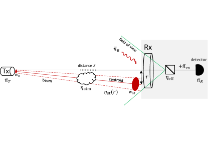
Figure 1: Free-space communication from a transmitter (Tx) to a receiver (Rx) separated by distance $z$. The transmitter generates a Gaussian beam with spot-size $w_{0}$ and mean number of photons $\bar{n}_{T}$. The propagation of the beam is affected by diffraction, atmospheric extinction $\eta_{\text{atm}}$, and turbulence/pointing errors, so that its short-term spot-size $w_{\text{st}}$ is randomly deflected by $r$ from the aperture center of the receiver, with an associated transmissivity $\eta_{\text{st}}(r)$. The beam is also affected by an additional attenuation, given by the efficiency $\eta_{\text{eff}}$ of the receiver. In total, transmitter and receiver are connected by an instantaneous lossy channel with transmissivity $\tau(r)=\eta_{\text{st}}(r)\eta_{\text{atm}}\eta_{\text{eff}}$ as in Eq. (17). Besides loss, we also consider noise. In particular, thermal noise $\bar{n}_{B}$ is collected by the field of view of the Rx and further noise $\bar{n}_{\text{ex}}$ may be locally generated by setup imperfections. As a result, the detector is hit by $\bar{n}_{R}=\tau(r)\bar{n}_{T}+\bar{n}$ mean photons whose $\bar{n}=\eta_{\text{eff}}\bar{n}_{B}+\bar{n}_{\text{ex}}$ are due to thermal noise.

As also depicted in Fig. 1, for each value of the deflection $r$, there is an associated transmissivity

$$\tau(r)=\eta_{\text{st}}(r)\eta_{\text{atm}}\eta_{\text{eff}},$$ (17)

where $\eta_{\text{st}}(r)$ accounts for the misalignment and reads

$$\eta_{\text{st}}(r)=e^{-\frac{4r^{2}}{w_{\text{st}}^{2}}}Q_{0}\left(\frac{2r^{2}}{w_{\text{st}}^{2}},\frac{4ra_{R}}{w_{\text{st}}^{2}}\right).$$ (18)

In the expression above, the factor $Q_{0}(x,y)$ is an incomplete Weber integral Agrest

$$Q_{0}(x,y):=(2x)^{-1}e^{x}\int_{0}^{y}dt~{}te^{-t^{2}/4x}I_{0}(t),$$ (19)

where the notation $I_{n}$ denotes a modified Bessel function of the first kind with order $n$. Note that Eq. (18) is obtained by adapting a previous result (Vasy12, , Eq. (D2)).

Following Ref. Vasy12 , we have that $\eta_{\text{st}}(r)$ can be well-approximated by the analytical expression

$$\eta_{\text{st}}(r)\simeq\eta_{\text{st}}\exp\left[-\left(\frac{r}{r_{0}}\right)^{\gamma}\right],$$ (20)

where $\gamma$ and $r_{0}$ are shape and scale (positive) parameters, given by the following functionals

$$\gamma =\frac{4\eta_{\text{st}}^{\text{far}}\Lambda_{1}(\eta_{\text{st}}^{\text{far}})}{1-\Lambda_{0}(\eta_{\text{st}}^{\text{far}})}\left[\ln\frac{2\eta_{\text{st}}}{1-\Lambda_{0}(\eta_{\text{st}}^{\text{far}})}\right]^{-1},$$ (21)

$$r_{0} =a_{R}\left[\ln\frac{2\eta_{\text{st}}}{1-\Lambda_{0}(\eta_{\text{st}}^{\text{far}})}\right]^{-\frac{1}{\gamma}},$$ (22)

with $\Lambda_{n}(x):=\exp\left(-2x\right)I_{n}\left(2x\right)$. As a result, combining Eqs. (17) and (20), we may write

$$\tau(r)=\eta\exp\left[-\left(\frac{r}{r_{0}}\right)^{\gamma}\right].$$ (23)

II.3.3 Incorporating beam wandering

Beam wandering is modelled by treating the position of the centroid as a stochastic variable, which can be taken to be Gaussian Dowling with variance $\sigma^{2}$ around the center of the receiver’s aperture, where $\sigma^{2}$ is the sum of two independent contributions: the variance $\sigma_{\text{TB}}^{2}$ due to large-scale turbulence, and the variance $\sigma_{\text{P}}^{2}$ due to pointing error. In general, one may also assume that the wandering is around an average deflection point at a non-zero distance $d$ from the center of the receiver’s aperture. For the sake of simplicity, here we consider the optimal working condition of $d=0$, which can always be realized by means of sufficiently-fast adaptive optics.

The Gaussian random walk around the receiver’s center induces a Weibull distribution for the deflection $r$, expressed by the zero-mean density function

$$P_{\text{WB}}(r)=\frac{r}{\sigma^{2}}\exp\left(-\frac{r^{2}}{2\sigma^{2}}\right).$$ (24)

In turn, the Weibull distribution over $r$ induces a corresponding probability density for $\tau=\tau(r)$, given by

$$P_{0}(\tau)=\frac{r_{0}^{2}}{\gamma\sigma^{2}\tau}\left(\ln\frac{\eta}{\tau}\right)^{\frac{2}{\gamma}-1}\exp\left[-\frac{r_{0}^{2}}{2\sigma^{2}}\left(\ln\frac{\eta}{\tau}\right)^{\frac{2}{\gamma}}\right],$$ (25)

as also discussed in Appendix D.

The random fluctuation of the effective transmissivity $\tau$ creates a fading channel from transmitter to receiver that can be described by the ensemble $\mathcal{E}:=\{P_{0}(\tau),\mathcal{E}_{\tau}\}$, where the lossy channel $\mathcal{E}_{\tau}$ with transmissivity $\tau$ is randomly selected with probability density $P_{0}(\tau)$. Using the convexity properties of the relative entropy of entanglement (REE) REE1 ; REE2 ; REE3 over an ensemble of channels as in Ref. (QKDpaper, , Eq. (17)), we can bound the secret key capacity of the fading channel $\mathcal{E}$ by means of the following average

$$K\leq\int_{0}^{\eta}d\tau~{}P_{0}(\tau)\Phi(\tau):=\mathcal{B}(\eta,\sigma),$$ (26)

where $\Phi(\tau)=-\log_{2}(1-\tau)$ is the PLOB bound associated with the instantaneous channel $\mathcal{E}_{\tau}$.

The integral in Eq. (26) can be simplified by working with the variable $\ln(\eta/\tau)$ and then solving by parts. In this way, we find that the maximum secret key rate achievable through the free-space channel is bounded by

$$K\leq\mathcal{B}(\eta,\sigma)=-\Delta(\eta,\sigma)\log_{2}(1-\eta),$$ (27)

where the correction factor $\Delta$ is given by

$$\Delta(\eta,\sigma)=1+\frac{\eta}{\ln(1-\eta)}\int_{0}^{+\infty}dx\frac{\exp\left(-\frac{r_{0}^{2}}{2\sigma^{2}}x^{2/\gamma}\right)}{e^{x}-\eta}.$$ (28)

The formula in Eq. (27) is our main result: It bounds the secret key capacity $K$ and the entanglement-distribution capacity $E$ of a free-space lossy channel $\mathcal{E}$ affected by diffraction, extinction, setup-loss, and fading, the latter being induced by turbulence and pointing errors.

We can further simplify the upper bound $\mathcal{B}(\eta,\sigma)$ for high loss $\eta\ll 1$. In fact, in such a case, we can reduce the $\Delta$-correction and write the approximate bound

$$\mathcal{B}(\eta,\sigma) \simeq\frac{\eta\Lambda(\eta,\sigma)}{\ln 2},$$ (29)

$$\Lambda(\eta,\sigma) :=1-\int_{0}^{+\infty}dx~{}\exp\left(-\frac{r_{0}^{2}}{2\sigma^{2}}x^{2/\gamma}-x\right)$$ (30)

Note that the condition $\eta\ll 1$ is not necessarily achieved in the far field, because $\eta=\eta_{\text{st}}\eta_{\text{atm}}\eta_{\text{eff}}$ and the factors $\eta_{\text{atm}}\eta_{\text{eff}}$ may decrease the overall value of the transmissivity already in the near field. In the far field ($z\gg z_{R}$), we may use both $\eta\ll 1$ and the expansion $\eta_{\text{st}}\simeq 2a_{R}^{2}w_{\text{st}}^{-2}$, so that we can write

$$\mathcal{B}(\eta,\sigma)\simeq\frac{\eta_{\text{atm}}\eta_{\text{eff}}}{\ln 2}\frac{2a_{R}^{2}}{w_{\text{st}}^{2}}\Lambda(\eta,\sigma).$$ (31)

In our model above, the free-space channel $\mathcal{E}$ is an ensemble $\{P_{0}(\tau),\mathcal{E}_{\tau}\}$ of instantaneous pure-loss channels $\mathcal{E}_{\tau}$ with probability $P_{0}(\tau)$. For all these channels the upper bound $\Phi(\tau)$ is achievable by their (bosonic) reverse coherent information RCI ; CInfo , which corresponds to the optimal rate of entanglement distribution protocols assisted by one-way classical communication (see Appendix E for details). Averaging over $P_{0}(\tau)$ implies that the upper bound in Eq. (27) is achievable by these entanglement distribution protocols and, therefore, we may write $E=K=-\Delta\log_{2}(1-\eta)$, where $E\leq K$ is the entanglement distribution capacity of the link.

In conclusion, as long as we can neglect thermal noise and consider a pure-loss fading process, the bound in Eq. (27) represents both the secret-key and entanglement distribution capacity of the free-space link. In particular, note that the formulas in Eqs. (27) and (29) have a clear structure. They are given by the capacity $-\log_{2}(1-\eta)\simeq\eta/\ln 2$ achievable with a perfectly-aligned link with no wandering, multiplied by a free-space correction factor which accounts for the wandering effects ($\Delta\simeq\Lambda$).

One can check that, with the assumptions of negligible turbulence and pointing error (so that $\sigma\simeq 0$ and $\eta_{\text{st}}\simeq\eta_{\text{d}}$), we have $\Delta\simeq 1$ in Eq. (28), and Eq. (27) reduces to Eq. (8). If we further assume no atmospheric extinction and unit setup efficiency, Eq. (27) reduces to Eq. (3) which only accounts for free-space diffraction.

II.4 Thermal noise

The quantity $-\Delta\log_{2}(1-\eta)$ in Eq. (27) provides an upper bound even in the presence of thermal noise. The reason is because any instantaneous thermal-loss channel $\mathcal{E}_{\tau,\bar{n}}$ adding a mean number of photons $\bar{n}$ can be written as a decomposition of a pure-loss channel $\mathcal{E}_{\tau}$ followed by a suitable additive-Gaussian noise channel RMP . Because the PLOB bound $\Phi$ is based on the REE, it is monotonic over such decompositions, so that its value $\Phi(\tau,\bar{n})$ computed over $\mathcal{E}_{\tau,\bar{n}}$ cannot exceed its value $\Phi(\tau)$ over $\mathcal{E}_{\tau}$. Thus, the loss-based upper bound in Eq. (27) is still valid in the presence of thermal noise (no matter if this noise is trusted or untrusted). However, it is no longer guaranteed to be achievable. For this reason, we derive a tighter upper bound and a corresponding lower bound (technical details about the following derivations are in Appendix F).

Assume that the receiver collects a non-trivial amount of thermal noise which couples into the output mode. The natural source is the brightness of the sky $B_{\lambda}^{\text{sky}}$ which varies between $\simeq 1.5\times 10^{-6}$ and $\simeq 1.5\times 10^{-1}$ W m^-2 nm^-1 sr^-1, from clear night to cloudy day-time Miao (and assuming that the field of view does not include the Moon or the Sun). For a receiver with aperture $a_{R}$, angular field of view $\Omega_{\text{fov}}$, and using a detector with time window $\Delta t$ and spectral filter $\Delta\lambda$ around $\lambda$, the number of background thermal photons per mode is given by Miao ; BrussSAT

$$\bar{n}_{B}=\frac{\pi\lambda\Gamma_{R}}{hc}B_{\lambda}^{\text{sky}},~{}\Gamma_{R}:=\Delta\lambda\Delta t\Omega_{\text{fov}}a_{R}^{2},$$ (32)

where $h$ is Planck’s constant and $c$ is the speed of light.

As an example, for a $100~{}$MHz detector ($\Delta t=10~{}$ns) with a filter $\Delta\lambda=1~{}$nm around $\lambda=800~{}$nm, and a telescope with $a_{R}=5~{}$cm and $\Omega_{\text{fov}}=10^{-10}~{}$sr, the value of $\bar{n}_{B}$ ranges between $\simeq 4.75\times 10^{-8}$ photons/mode (at night) and $\simeq 4.75\times 10^{-3}$ photons/mode (during a cloudy day). A fraction $\eta_{\text{eff}}\bar{n}_{B}$ of these photons is detected by a receiver with limited efficiency $\eta_{\text{eff}}$. See Fig. 1.

It is important to note that the number of photons in the natural background $\bar{n}_{B}$ may be higher than that expected from Eq. (32), as a consequence of the presence of bright sources of light within the field of view of the receiving telescope. Our formalism accounts for such deviations, even though we consider Eq. (32) in our numerical simulations. In general, all the (detected) photons coming from the outside channel must be ascribed to Eve in the worst-case scenario, even though this is a over-pessimistic assumption due to the line-of-sight configuration in free-space communication. However, such an assumption must be made because Eve might inject and hide her photons in the background.

Besides the natural background, excess photons $\bar{n}_{\text{ex}}$ may be created by imperfections in the receiver setup (e.g., due to electronic noise and other errors), so that the receiver sees a total of $\bar{n}=\eta_{\text{eff}}\bar{n}_{B}+\bar{n}_{\text{ex}}$ thermal photons. Thus, assuming that $\bar{n}_{T}$ mean photons are generated at the transmitter and $\tau$ is the overall instantaneous transmissivity of the channel, the receiver’s detector gets $\bar{n}_{R}=\tau\bar{n}_{T}+\bar{n}$ mean photons (per mode). See Fig. 1.

The free-space process in Fig. 1 can be described by an overall thermal-loss channel $\mathcal{E}_{\tau,\bar{n}}$ with instantaneous transmissivity $\tau$ and output thermal noise $\bar{n}$. This channel is equivalent to a beam-splitter mixing the signal mode with an input thermal mode with $\bar{n}_{e}:=\bar{n}(1-\tau)^{-1}$ mean photons. In the worst-case scenario, Eve controls all the input noise and collects all the photons that are leaked from the other output of the beam-splitter (which means that she collects photons leaking from both the channel and the receiver setup).

In order to account for the centroid wandering, we adopt the distribution $P_{0}(\tau)$ for the transmissivity $\tau$ while keeping the output thermal noise $\bar{n}$ as a constant. The latter is in fact composed of a fraction $\bar{n}_{B}$ which is independent from the fading process, while the other contribution $\bar{n}_{\text{ex}}$ can always be assumed to be optimized over such a process (see discussion in Appendix F.1 for more details). For this reason, the free-space fading channel can be represented by the ensemble $\mathcal{E}=\{P_{0}(\tau),\mathcal{E}_{\tau,\bar{n}}\}$.

For a free-space fading channel $\mathcal{E}$ with maximum transmissivity $\eta$ and thermal noise $\bar{n}\leq\eta$, we compute the following tighter upper bound for the secret key capacity

$$K\leq-\Delta(\eta,\sigma)\log_{2}(1-\eta)-\mathcal{T}(\bar{n},\eta,\sigma),$$ (33)

where the thermal correction $\mathcal{T}$ is given by

$$\mathcal{T}(\bar{n},\eta,\sigma) =\left\{1-e^{-\frac{r_{0}^{2}}{2\sigma^{2}}\left[\ln\left(\eta/\bar{n}\right)\right]^{2/\gamma}}\right\}\left[\frac{\bar{n}\log_{2}\bar{n}}{1-\bar{n}}+h\left(\bar{n}\right)\right]$$

$$-\Delta(\bar{n},\sigma)\log_{2}(1-\bar{n}),$$ (34)

and we have used the entropic function

$$h\left(x\right):=(x+1)\log_{2}(x+1)-x\log_{2}x.$$ (35)

We also compute the following achievable rate (lower bound) for entanglement distribution and, therefore, secret key generation

$$E\geq-\Delta(\eta,\sigma)\log_{2}(1-\eta)-h\left(\frac{\bar{n}}{1-\eta}\right).$$ (36)

For negligible noise $\bar{n}$, the bounds in Eqs. (33) and (36) collapse to the bound in Eq. (27). By contrast, for strong noise $\bar{n}=\eta$, the thermal correction in Eq. (34) becomes predominant and we get $K\leq 0$ from Eq. (33). The threshold condition $\bar{n}=\eta$ implies the existence of a maximum security distance $z_{\text{max}}$ for free-space QKD in the presence of thermal noise. A simple bound on this maximum distance is achieved imposing $\bar{n}=\eta_{\text{d}}$. In fact, for a collimated beam, this leads to

$$2f_{0R}(z_{\max})\geq-\ln(1-\bar{n}),$$ (37)

where $f_{0R}$ is the Fresnel number product of the beam and the receiver (see Sec. II.1).

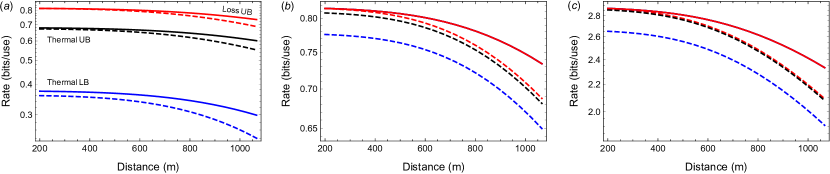
Figure 2: Performance of free-space quantum communications in terms of bits per channel use versus distance. (a) We consider the general worst-case scenario with untrusted loss and noise at the receiver ($\eta_{\text{eff}}=0.5$, $\bar{n}_{\text{ex}}=0.05$). We plot the ultimate loss-based upper bound of Eq. (27) for night time (top red line) and day time (red dashed line). This is compared with the bounds explicitly accounting for thermal noise $\bar{n}=\eta_{\mathrm{eff}}\bar{n}_{B}+\bar{n}_{\mathrm{ex}}$. In particular, we plot the thermal upper bound of Eq. (33) for night time (black solid line) and day time (black dashed line), as well as the thermal lower bound of Eq. (36) for night time (blue solid line) and day time (blue dashed line). (b) Same comparison as in (a) but considering a noise-less receiver ($\eta_{\text{eff}}=0.5$, $\bar{n}_{\text{ex}}=0$). For night time, the upper- and lower- thermal bounds coincide with loss-based upper bound (solid red line). For day time, the performances are instead separate (dashed lines). (c) Same comparison as in (a) but considering an ideal loss-less and noise-less receiver ($\eta_{\text{eff}}=1$, $\bar{n}_{\text{ex}}=0$). As in (b), the two thermal bounds collapse in the loss-based upper bound during night time (solid red line). Performances are different during day time (dashed lines). Other parameters are: $R_{0}=\infty$ (collimated Gaussian beam), $\lambda=800~{}$nm, $w_{0}=a_{R}=5~{}$cm, $\Omega_{\text{fov}}=10^{-10}~{}$sr, $\Delta t=10~{}$ns and $\Delta\lambda=1~{}$nm. We consider $h=30~{}$m, so that $C_{n}^{2}\simeq 1.28(2.06)\times 10^{-14}~{}$m^-2/3 for night (day), and we have $\bar{n}_{B}\simeq 4.75\times 10^{-8}$ ($\times 10^{-3}$) at night (cloudy day).

II.5 Analysis of the ultimate bounds

In order to study our bounds, we consider different possibilities which depend on the treatment of loss and noise present in the setup of the receiver. In the worst-case scenario assumed so far, we explicitly account for the non-ideal values of the receiver parameters $\eta_{\text{eff}}$ and $\bar{n}_{\text{ex}}$, assuming that Eve may access that leakage and control that noise. This setting can be used to bound the performance of all protocols where both leakage and local noise in the receiving setup are considered to be untrusted. We may then consider the case where the local noise $\bar{n}_{\text{ex}}$ is set to zero, i.e., a noiseless-receiver. This setting can be used to bound all protocols where such local noise is considered to be trusted (trusted-noise scenario). Finally, we may also consider the optimal case of $\bar{n}_{\text{ex}}=0$ and $\eta_{\text{eff}}=1$, i.e., an ideal loss-less and noise-less receiver. This can be used to bound all those protocols where local noise and limited efficiency of the receiver are both considered to be trusted (trusted-loss-and-noise scenario).

Numerical behavior of the bounds is shown in Fig. 2. For the chosen parameters, the condition of weak turbulence $\sigma_{\text{Rytov}}^{2}<1$ limits day-time distance to a range of $z\lesssim 1~{}$km. As we can see from Fig. 2(a), there is a clear gap between the ultimate loss-based upper bound of Eq. (27) and the two thermal bounds in Eqs. (33) and (36). This is created by the presence of thermal noise $\bar{n}$. During the night, when the background contribution $\bar{n}_{B}$ is negligible, it is the presence of untrusted setup noise $\bar{n}_{\text{ex}}$ to create the gap in the performances [see solid lines in Fig. 2(a)]. During the day, there is a higher turbulence on the ground as quantified by the higher value of the structure constant $C_{n}^{2}$; mainly for this reason, we have a degradation of all the day-time rates with respect to their night-time counterparts [compare dashed with solid lines in Fig. 2(a)]. For the thermal bounds this degradation is slightly increased due to the additional contribution of the thermal background $\bar{n}_{B}$, which is non-negligible during the day.

In the case of a noise-less receiver as in Fig. 2(b), thermal noise is only coming from the external background $\bar{n}_{B}$. For night-time operation, this background is negligible and the two thermal bounds in Eqs. (33) and (36) collapse into the loss-bound of Eq. (27), which therefore represents the secret key capacity (and entanglement distribution capacity) of the night-time link [see red solid line in Fig. 2(b)]. However, during the day, the external background $\bar{n}_{B}$ is not negligible and this creates a small gap in the performance, so that there is no collapse of the thermal bounds [black and blue dashed lines in Fig. 2(b)] into the upper loss-based bound [red dashed line in Fig. 2(b)]. In the case of an ideal (loss- and noise-less) receiver, we have basically the same situation but with higher rates, as shown in Fig. 2(c).

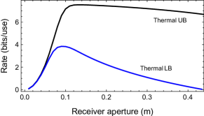
Figure 3: For day time and fixed distance $z=1~{}$km, we plot the thermal bounds in Eqs. (33) and (36) as a function of the receiver’s aperture $a_{R}$. We assume an ideal receiver ($\bar{n}_{\text{ex}}=0$ and $\eta_{\text{eff}}=1$). Other parameters are as in Fig. 2.

An interesting observation for day-time operation is the trade-off between Eq. (15), where $a_{R}$ increases the transmissivity, and Eq. (32), where $a_{R}$ increases thermal noise. For this reason, the optimal performance is achieved when the receiver’s aperture $a_{R}$ takes an intermediate value. For instance consider the case of an ideal receiver, and let us study the behavior of the two thermal bounds in Eqs. (33) and (36) as a function of $a_{R}$ at some fixed distance, say $z=1$ km. As we can see from Fig. 3 we find an optimal working point at around $a_{R}\simeq 10~{}$cm for the specific regime considered. This is true as long as the other parameters of the receiver are fixed, such as its field of view $\Omega_{\text{fov}}$ which intervenes in Eq. (32). Note that the field of view does not directly depend on $a_{R}$, but decreases with the focal length of the receiver’s telescope $f$ and increases with the area of the detector $a$. For instance, for a rectilinear optical system focused at $\infty$, it is easy to check that the angle of view satisfies $\Omega_{\text{fov}}^{1/2}$ $\simeq 2\arctan[\sqrt{a}/(2f)]$, which is also a good approximation for a spherical optical system.

II.5.1 Noise filtering

It is important to note that the behavior of the thermal bounds is strongly dependent on the filter $\Delta\lambda$. So far, numerical investigations have assumed a value of $\Delta\lambda=1~{}$nm, which is the value of the narrow-band filter typically considered in studies with discrete variables. At $800~{}$nm, the value $\Delta\lambda=1~{}$nm corresponds to a relatively-large bandwidth of $\Delta\nu=c\lambda^{-2}\Delta\lambda\simeq 470~{}$GHz. However, in the setting of continuous variables, much narrower filters are possible by exploiting suitable interferometric procedures at the receiver, so that the effective value of $\Delta\nu$ becomes equivalent to the bandwidth of the transmitted pulses.

An important ingredients in experiments with CV systems is the local oscillator (LO). They are typically performed with a transmitted LO (TLO), where each quantum signal is multiplexed in polarization with an associated LO and both are sent to the receiver. At the receiver, signal and LO are demultiplexed via a polarizing beam splitter and made interfered on a beam splitter before detection (in a homodyne or heterodyne setup). Alternatively, CV experiments may be performed with a local local oscillator (LLO), where quantum signals are interleaved with strong reference pulses, the latter being used by the receiver to reconstruct the local oscillator “locally” (with some imperfection LLO ; LLO2 ).

It is important to note that, in a homodyne measurement, the output of the detector is proportional to $\sqrt{\bar{n}_{\text{LO}}}\hat{x}$, where $\hat{x}$ is the generic quadrature of the signal and $\bar{n}_{\text{LO}}$ is the number of photons from the LO. The value of $\bar{n}_{\text{LO}}$ can be very high. In fact, considering $10~{}$ns-long pulses from a $100$ mW laser at $\lambda=800~{}$nm, we have that each pulse contains $\bar{n}_{\text{LO}}\simeq 4\times 10^{9}$ photons. Even if we pessimistically assume $20$dB of loss ($\tau\simeq 10^{-2}$), we see that about $\mathcal{O}(10^{7})$ photons reach the receiver.

Thanks to the large pre-factor $\sqrt{\bar{n}_{\text{LO}}}$, only the contribution of thermal noise mode-matching with the LO will survive in the output. This means that the interferometric process introduces an effective filter which is given by the bandwidth $\Delta\nu$ of the LO. Compatibly with the time-bandwidth product $\Delta t\Delta\nu\geq 0.44$ (for Gaussian pulses), one can make $\Delta\nu$ very small. As an example, for a $10~{}$ns pulse, we may consider $\ \Delta\nu=50~{}$MHz corresponding to just $\Delta\lambda=0.1~{}$pm around $800$ nm; this filter is $4$ orders of magnitude narrower than the one considered above. With respect to $\Delta\lambda=1~{}$nm, such a narrow filter realizes a corresponding $10^{-4}$ suppression of the background noise $\bar{n}_{B}$, which therefore becomes negligible (day-time noise becomes $\bar{n}_{B}\simeq 10^{-7}$). As a result, the detector would only experience locally-generated noise, i.e., $\bar{n}\simeq\bar{n}_{\text{ex}}$.

From the point of view of the rates, with a narrow filter $\Delta\lambda=0.1~{}$pm, we have an increase of the day-time thermal bounds in Fig. 2. In particular, for a noise-less setup ($\bar{n}_{\text{ex}}=0$) we have $\bar{n}\simeq 0$. In this case, the day-time thermal bounds computed from Eqs. (33) and (36) collapse into the day-time loss-bound given by Eq. (27), which therefore becomes the secret-key capacity (and entanglement distribution capacity) of the day-time link. This means that the black and blue dashed lines in Fig. 2(b) collapse into the upper red dashed line. The same happens in Fig. 2(c) which refers to a loss-less and noise-less setup, but with higher rates.

It is worth stressing that, if we optimize over the receiver so to make the total thermal noise $\bar{n}$ negligible (as a result of a noise-less setup $\bar{n}_{\text{ex}}\simeq 0$ and noise-filtering $\bar{n}_{B}\simeq 0$), then the loss-bound of Eq. (27) is achievable no matter what the external conditions are (night- or day-time). It is also clear that this bound can be further optimized by assuming no pointing error at the transmitter and unit quantum efficiency at the receiver. The result of these optimizations (implicit in our formula) provides a bound/capacity which uniquely depends on the external free-space channel between the two remote parties (affected by diffraction, extinction and turbulence).

II.6 Extension of the bounds

II.6.1 Slow detection

So far, we have considered the situation where the detector of the receiver is fast enough to resolve the wandering of the centroid. In general, this dynamics has two components: on the one hand, there are the fluctuations induced by atmospheric turbulence, with a time scale of the order of 10-100 ms; on the other hand, there is pointing error (from jitter and imprecise tracking) that fluctuates over a slightly slower time scale, of the order of 0.1-1 s. For detection, we can therefore identify three different regimes: (i) fast detectors able to resolve all the dynamics above; (ii) intermediate detectors, able to solve part of the dynamics, i.e., pointing-error wandering but not turbulence-induced fluctuations; and (iii) slow detectors, not able to resolve any of the wandering dynamics. For instance, the latter situation may occur when the measurement time is intentionally increased with the aim of increasing the detection efficiency. In all cases, we assume that the pulses have a temporal length perfectly matching the bandwidth of the detector.

In the case of an intermediate detector (ii), we integrate over the fast fading process induced by turbulence. As a result, we have an overall fading channel which is only generated by the pointing error, and whose instantaneous transmissivity is now determined by the long-term spot size $w_{\text{lt}}^{2}=w_{\text{st}}^{2}+\sigma_{\text{TB}}^{2}$. Let us set

$$\eta_{\text{int}} =\eta_{\text{lt}}\eta_{\text{atm}}\eta_{\text{eff}},$$ (38)

$$\eta_{\text{lt}} :=1-\exp\left(-2a_{R}^{2}/w_{\text{lt}}^{2}\right)\simeq\frac{2a_{R}^{2}}{w_{\text{lt}}^{2}}:=\eta_{\text{lt}}^{\text{far}}.$$ (39)

Then we may write the upper bound

$$K_{\text{int}}\leq\mathcal{B}_{\text{int}}:=-\Delta(\eta_{\text{int}},\sigma_{\text{P}})\log_{2}(1-\eta_{\text{int}}),$$ (40)

where $\Delta$ of Eq. (28) has to be computed over $\eta_{\text{int}}$ and $\sigma_{\text{P}}$ (with parameters $r_{0}$ and $\gamma$ to be computed over $\eta_{\text{lt}}$ and $\eta_{\text{lt}}^{\text{far}}$). Similarly, the thermal upper bound takes the form

$$K_{\text{int}}\leq\mathcal{B}_{\text{int}}-\mathcal{T}(\bar{n},\eta_{\text{int}},\sigma_{\text{P}}).$$ (41)

Basically, we obtain the modified formulas by setting $\sigma_{\text{TB}}^{2}\simeq 0$ and replacing $w_{\text{st}}$ with the long-term spot size $w_{\text{lt}}$ in the bounds of Eqs. (27), (33) and (36).

Assuming a slower detector (iii), we need to integrate over the entire fading process induced by turbulence and pointing error. Instead of a fading channel, we now have an average lossy channel with transmissivity $\eta_{\text{tot}}$ which is determined by the long-term spot size $w_{\text{lt}}^{2}=w_{\text{st}}^{2}+\sigma_{\text{TB}}^{2}$ together with the variance of the pointing error $\sigma_{\text{P}}^{2}$, besides $\eta_{\text{atm}}$ and $\eta_{\text{eff}}$. In other words, we have NoteIntegral

$$\eta_{\text{tot}} =\left[1-\exp\left(-2a_{R}^{2}/w_{\text{tot}}^{2}\right)\right]\eta_{\text{atm}}\eta_{\text{eff}},$$ (42)

$$w_{\text{tot}}^{2} :=w_{\text{lt}}^{2}+\sigma_{\text{P}}^{2}=w_{\text{st}}^{2}+\sigma_{\text{TB}}^{2}+\sigma_{\text{P}}^{2}.$$ (43)

As a result, the upper bound in Eq. (27) simplifies to

$$K_{\text{slow}}\leq-\log_{2}(1-\eta_{\text{tot}})\leq\frac{2}{\ln 2}\frac{a_{R}^{2}}{w_{\text{lt}}^{2}+\sigma_{\text{P}}^{2}}.$$ (44)

Similarly, the thermal upper bound of Eq. (33) becomes

$$K_{\text{slow}} \leq-\log_{2}\left[(1-\eta_{\text{tot}})\eta_{\text{tot}}^{\overline{n}^{\ast}}\right]-h\left(\overline{n}^{\ast}\right),$$ (45)

$$\overline{n}^{\ast} :=\bar{n}/(1-\eta_{\text{tot}}),$$ (46)

for $\bar{n}\leq\eta_{\text{tot}}$, and is equal to zero otherwise. Note that this formula is a direct modification of Ref. (QKDpaper, , Eq. (23)).

It is important to note that, in order to fairly compare Eqs. (40), (41), (44) and (45) with the previous fast-detection bounds, we need to account for the clock of the system. In fact, in such a comparison, one should explicitly account for the integration time which smooths the fluctuations but also reduces the final rate (or throughput) in terms of bits per second. In fact, given a rate $K$ in terms of bits/use, we need to plug a clock $C$ (uses/second) which depends on the bandwidth of the detector and the repetition rate of the source. The effective rate (bits/second) would then be $CK$. For instance, using a detector with bandwidth $W=100$ MHz, we may work with $10~{}$ns pulses and use a clock of $C=W/3\simeq 3.3\times 10^{7}$ uses (pulses) per second. If we assume a slow detector (and corresponding longer pulses) with a detection time of $100$ ms, we then have a clock of about $3.3$ uses per second, leading to orders-of-magnitude lower rate in terms of bits per second. Furthermore, long detection times also lead to higher background noise, which may become a major problem for day time.

II.6.2 Intermediate and strong turbulence

The previous bounds for slow detection can be stated for increasing levels of turbulence. From a physical point of view, stronger values of turbulence can be associated with an increasingly-faster averaging process so that the receiver loses the ability to resolve the fading dynamics. The effect is similar to having an increasingly-slower detector. However, besides this averaging process, there is also the appearance of scintillation effects and other effects of beam deformation, so that the transition from weak to stronger regimes of turbulence cannot be described in simple mathematical terms. That being said, the concept of long-term spot size is robust and applies to the various regimes of turbulence, from weak to strong (Fante75, , Sec. IIIA). In fact, even when the beam is broken up in multiple patches (e.g., see case 4 of (Fante75, , Sec. IIIA)), the long-term spot size provides the mean square radius of the region containing the patches.

In virtue of these considerations, we may rely on the robustness of the notion of long-term spot size to extend our upper bounds beyond the weak ($\sigma_{\text{Rytov}}^{2}<1$) and the weak-intermediate ($\sigma_{\text{Rytov}}^{2}\simeq 1$) regimes of turbulence (see also Appendix C for a discussion of these regimes in terms of the ratio $\rho_{0}/w_{0}$). At intermediate-strong turbulence ($\sigma_{\text{Rytov}}^{2}>1$), the variance $\sigma_{\text{TB}}^{2}$ becomes relatively small, while the short-term spot size $w_{\text{st}}$ tends to approximate the long-term value $w_{\text{lt}}$. If the pointing error is non-negligible, then we may write the upper bounds in Eqs. (40) and (41). However, if pointing error $\sigma_{\text{P}}^{2}$ is also negligible (with respect to $w_{\text{lt}}^{2}$), then we directly consider the upper bounds in Eqs. (44) and (45). For high values of turbulence ($\sigma_{\text{Rytov}}^{2}\gg 1$), we may certainly assume $\sigma_{\text{P}}^{2}\simeq\sigma_{\text{TB}}^{2}\ll w_{\text{lt}}^{2}$, so that we write the upper bounds in Eqs. (44) and (45) for the strong-turbulence secret-key capacity $K_{\text{strong}}$. Because these bounds do not come from an operational reduction of the detection time, the value $C$ of the system of clock can be high here.

III Composable security and key rates for CV-QKD

In this second part of the manuscript we study practical rates for free-space CV-QKD, therefore providing state-of-the-art lower bounds for the free-space secret key capacities discussed in the first part of the manuscript (Sec. II). In this specific section, we first develop a general and simplified theory of composable security that applies to CV-QKD protocols with a stable channel (fixed transmissivity), as is the typical case in fiber-based implementations or even certain free-space links where turbulence and other fading effects are negligible. This theory is the basis for the next Sec. IV, where we extend it to the case of CV-QKD protocols over a fading channel (variable transmissivity) as is the general case of free-space links affected by pointing errors and turbulence. The latter is a more difficult scenario but with interesting implications for both ground- and satellite-based communications PirandolaSAT ; UsenkoSTRATEGY1 ; UsenkoSTRATEGY2 ; PanosFading ; LeverrierSAT ; RalphFREE ; Malaney ; Masoud .

III.1 Description of the protocol

Let us study a Gaussian-modulated coherent-state protocol with a fixed transmissivity between Alice (the transmitter) and Bob (the receiver) QKDreview . The general scenario is the one depicted Fig. 4. Alice encodes classical information in a bosonic mode by preparing a coherent state $\left|\alpha\right\rangle$ whose amplitude $\alpha$ is modulated according to a complex Gaussian distribution with zero mean and variance $\mu-1$. Note that we may write $\alpha=(q+ip)/2$, where $x=q$ or $p$ is the mean value of the generic quadrature operator $\hat{x}=\hat{q}$ or $\hat{p}$ with $[\hat{q},\hat{p}]=2i$ RMP . Therefore, the generic quadrature of the mode can be decomposed as $\hat{x}=\hat{x}_{0}+x$, where $\hat{x}_{0}$ corresponds to vacuum noise and the displacement $x$ is a real Gaussian variable with zero mean and variance $\sigma_{x}^{2}=\mu-1$.

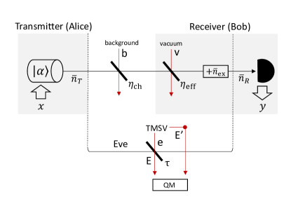
Figure 4: General description of the protocol and worst-case eavesdropping scenario. Alice’s modulated coherent state $\left|\alpha\right\rangle$, with $\bar{n}_{T}$ mean photons, is subject to channel loss $\eta_{\text{ch}}$ and background noise $\bar{n}_{B}$, before entering the receiver with quantum efficiency $\eta_{\text{eff}}$ and setup noise $\bar{n}_{\text{ex}}$. Bob’s detects $\bar{n}_{R}=\tau\bar{n}_{T}+\bar{n}$ mean photons, where $\tau=\eta_{\text{ch}}\eta_{\text{eff}}$ is the total transmissivity of the link and $\bar{n}=\eta_{\text{eff}}\bar{n}_{B}+\bar{n}_{\text{ex}}$ is the total number of thermal photons. The input-output relation for the quadratures is given by Eq. (48). In the worst-case scenario, Eve collects all the leakage and controls all thermal noise. This is equivalent to assume that she replaces the channel with a beam-splitter with transmissivity $\tau$ and thermal input $\bar{n}_{e}=\bar{n}/(1-\tau)$. The latter is part of a TMSV state in her hands, whose output is stored in a quantum memory.

The coherent state contains $\bar{n}_{T}=\left|\alpha\right|^{2}$ mean number of photons and it is transmitted through a channel with transmissivity $\eta_{\text{ch}}$ and environmental noise $\bar{n}_{b}=\bar{n}_{B}(1-\eta_{\text{ch}})^{-1}$, so that $\bar{n}_{B}$ thermal photons are injected in the channel. (In terms of the free-space configuration of Fig. 1, parameter $\eta_{\text{ch}}$ corresponds to the instantaneous value $\eta_{\text{atm}}\eta_{\text{st}}(r)$, and $\bar{n}_{B}$ is the thermal background.) The output state is then measured by a receiver with limited efficiency $\eta_{\text{eff}}$ and affected by thermal noise, such to add $\bar{n}_{\text{ex}}$ extra mean photons. As a result, the final (ideal) detection is reached by $\bar{n}_{R}=\tau\bar{n}_{T}+\bar{n}$ mean photons, where $\tau=\eta_{\text{ch}}\eta_{\text{eff}}$ is the total transmissivity and

$$\bar{n}=\eta_{\text{eff}}\bar{n}_{B}+\bar{n}_{\text{ex}}$$ (47)

is the total number of thermal photons. See Fig. 4.

The final detection is either a randomly-switched measurement of $\hat{q}$ or $\hat{p}$ (homodyne) or a joint measurement of $\hat{q}$ and $\hat{p}$ (heterodyne). In both cases, there is an outcome $y$ corresponding to Alice’s classical input $x$. A single pair $(x,y)$ per mode is generated by the homodyne protocol GG02 , while two pairs per mode are generated by the heterodyne protocol Noswitch . For both protocols, we may compactly write the input-output relation

$$y=\sqrt{\tau}x+z,$$ (48)

where the noise variable is given by

$$z =\sqrt{\eta_{\text{eff}}(1-\eta_{\text{ch}})}\hat{x}_{b}+\sqrt{\tau}\hat{x}_{0}$$

$$+\sqrt{1-\eta_{\text{eff}}}\hat{x}_{v}+\xi_{\text{ex}}+\xi_{\text{det}}.$$ (49)

Here $\hat{x}_{b}$ is the quadrature of the background thermal mode, $\hat{x}_{v}$ is the quadrature of a setup vacuum mode, $\xi_{\text{ex}}$ is a Gaussian variable with variance $2\bar{n}_{\text{ex}}$, and $\xi_{\text{det}}$ is an additional variable whose variance depends on the specific type of final detection, i.e., we have $\mathrm{var}(\xi_{\text{det}})=0$ for homodyne, and $\mathrm{var}(\xi_{\text{det}})=1$ for heterodyne. It is useful to introduce the “quantum duty” or “qu-duty” $\nu_{\text{det}}$ to pay by the detector, which is $\nu_{\text{det}}=1$ for homodyne (due to the vacuum noise in the state) and $\nu_{\text{det}}=2$ for heterodyne (which is increased due to the simultaneous measurements of the two conjugate quadratures). Thus, in total, the noise variable $z$ has variance

$$\sigma_{z}^{2}=2\bar{n}+\nu_{\text{det}}.$$ (50)

Alice and Bob’s mutual information $I(x:y)$ is the same in direct reconciliation (Bob inferring $x$ from $y$) and reverse reconciliation (Alice inferring $y$ from $x$). This is easy to compute under ideal post-processing techniques, able to reach the Shannon capacity of the additive-noise Gaussian channel. In fact, from $\mathrm{var}(y)=\tau\sigma_{x}^{2}+\sigma_{z}^{2}$ and $\mathrm{var}(y|x)=\sigma_{z}^{2}$, one derives

$$I(x:y)=\frac{\nu_{\text{det}}}{2}\log_{2}\left(1+\frac{\sigma_{x}^{2}}{\chi}\right),$$ (51)

where $\chi:=\sigma_{z}^{2}/\tau$ is the equivalent noise, given by

$$\chi=\frac{2\bar{n}_{B}}{\eta_{\text{ch}}}+\frac{\nu_{\text{det}}+2\bar{n}_{\text{ex}}}{\tau}.$$ (52)

In particular, note that the first term in Eq. (52) is the specific contribution of the channel to the excess noise

$$\varepsilon_{\text{ch}}:=\frac{2\bar{n}_{B}}{\eta_{\text{ch}}}=\frac{2(\bar{n}-\bar{n}_{\text{ex}})}{\tau}.$$ (53)

For the homodyne and heterodyne protocols, we may explicitly write

$$I^{\text{hom}}(x :y)=\frac{1}{2}\log_{2}\left(1+\frac{\tau\sigma_{x}^{2}}{2\bar{n}+1}\right),$$ (54)

$$I^{\text{het}}(x :y)=\log_{2}\left(1+\frac{\tau\sigma_{x}^{2}}{2\bar{n}+2}\right).$$ (55)

Before proceeding with the security analysis and the derivation of the asymptotic key rate, it is important to clarify the most relevant noise contributions that are present in the setup noise $\bar{n}_{\text{ex}}$. In our study, we assume the worst-case scenario where this noise is considered to be untrusted, even though it may be estimated or calibrated by the parties. This robust approach allows us to lower-bound the performances that are achievable by CV-QKD in general, including those situations where some of the setup noise is considered to be trusted (as it might be the case for some tolerable level of electronic noise).

III.2 Practical observations on the receiver setup

Here we discuss the contributions to the setup noise, that may be broken up as $\bar{n}_{\text{ex}}=\bar{n}_{\text{LO}}+\bar{n}_{\text{el}}+\bar{n}_{\text{other}}$, where $\bar{n}_{\text{LO}}$ are thermal photons generated by imperfection in the LO (phase errors), $\bar{n}_{\text{el}}$ is electronic noise, and $\bar{n}_{\text{other}}$ is any other uncharacterized and independent noise source that might appear in the setup (that we numerically neglect here). In general, the setup noise $\bar{n}_{\text{ex}}$ will depend on the channel transmissivity. Below we start by describing $\bar{n}_{\text{LO}}$ which has a different behavior depending on the type of LO. Afterwards, we discuss the expression of $\bar{n}_{\text{el}}$.

III.2.1 Local oscillator (TLO and LLO)

In order to encode and decode information with the quadratures of a bosonic mode, the reference frames of the transmitter and receiver need to be phase-locked. There are two possible ways to achieve this: either via a TLO or an LLO. In the experimental practice, the use of a TLO is the simplest solution. One the one hand, it introduces negligible phase error $\bar{n}_{\text{TLO}}\simeq 0$ and guarantees that the spatial modes of the signal and LO pulses are the same, so that the mode matching is ideal at the receiver. On the other hand, the fact that the LO transmitted together with the signal means that it may also be the subject of attacks. This problem can be mitigated by real-time monitoring of the LO intensity and properties, so as to match the values expected by the parties QKDreview .

The other solution of a LLO excludes channel attacks against the LO, but inevitably introduces non-trivial phase errors in the receiver setup. These phase errors provide a contribution to the excess noise equal to

$$\varepsilon_{\text{LLO}}\simeq 2\pi\sigma_{x}^{2}C^{-1}l_{\text{W}},$$ (56)

where $C$ is the clock and $l_{\text{W}}$ is the laser linewidth. This formula is derived from Ref. LLO assuming that signal pulses and LO-reference pulses are generated with the same coherence time $\tau_{\text{coh}}\simeq(\pi l_{\text{W}})^{-1}$. More generally, in Eq. (56) one needs to consider the average linewidth $(l_{\text{W}}^{\text{signal}}+l_{\text{W}}^{\text{LO}})/2$, but we omit this technicality here.

From the formula, it is clear that the noise decreases for higher clocks and narrower linewidths. In general, this approach requires better hardware than the TLO. In our analysis, we have $\sigma_{x}^{2}\lesssim 10$, so that a reasonably low value $\varepsilon_{\text{LLO}}\lesssim 0.02$ can be reached by $C=5~{}$MHz and $l_{\text{W}}\simeq 1.6$ KHz or, alternatively, by $C=100~{}$MHz and $l_{\text{W}}\simeq 32$ KHz (e.g., together with a $1$ GHz homodyne receiver for detecting $0.1C^{-1}\simeq 1$ ns pulses NoteCLOCK ). In other words, very good cw-lasers and detectors are needed. Refined analyses suggest that highly-performant amplitude modulators are also required in order to avoid the introduction of other noise contributions LLO2 ; LLO3 .

To account for the LLO in our theoretical treatment, we recall that Alice and Bob’s mutual information takes the form in Eq. (51) where the equivalent noise $\chi$ is broken down as in Eq. (52), i.e., we write

$$\chi=\varepsilon_{\text{ch}}+\frac{\nu_{\text{det}}+2\bar{n}_{\text{ex}}}{\tau},$$ (57)

where $\varepsilon_{\text{ch}}:=2\bar{n}_{B}/\eta_{\text{ch}}$ is channel’s excess noise. The introduction of the LLO contribution consists of making the replacement $\chi\rightarrow\chi+\varepsilon_{\text{LLO}}$ in the formula above. Because this type of noise is within the local setup of the receiver, we make it a contribution to $\bar{n}_{\text{ex}}$ by writing

$$\bar{n}_{\text{LLO}}=\frac{\tau\varepsilon_{\text{LLO}}}{2}=\pi\tau\sigma_{x}^{2}C^{-1}l_{\text{W}}.$$ (58)

Some observations are in order. The basic implementation of LLO considers the regular alternation between signal and LO-reference pulses. In such a setting, one may argue that the actual rate per second (throughput) is halved with respect to the TLO. However, it is worth noticing that this factor $1/2$ may be compensated if the signals are encoded in both polarizations for each channel use (not possible for a TLO due to its multiplexing in polarization). Another observation is about the use of homodyne or heterodyne at the receiver. Because of the regular signal-reference alternation, the receiver may use a dedicated heterodyne detector for the LO references and another detector for the signals (heterodyne or randomly-switched homodyne). However, if the receiver is limited to a single homodyne detector, then the transmitter can send two LO-reference pulses with orthogonal polarizations and rotated by $\pi/2$ in phase space. At the receiver, these pulses can be demultiplexed, delayed and sequentially homodyned to give the complete phase information.

III.2.2 Electronic noise

One of the typical and unavoidable sources of noise within the setup of the receiver is electronic noise, with associated variance $\nu_{\text{el}}$ or equivalent number of photons $\bar{n}_{\text{el}}=\nu_{\text{el}}/2$. This depends on the noise equivalent power (NEP) of the amplifiers and photodiodes to be used in the homodyne detectors, besides the detection bandwidth $W$, the duration of the LO pulses $\Delta t_{\text{LO}}$, the LO power at the detector $P_{\text{LO}}^{\text{det}}$, and the frequency of the light $\nu$. In fact, one can write the formula elenoise1 ; elenoise2

$$\nu_{\text{el}}=\frac{\nu_{\text{det}}\mathrm{NEP}^{2}W\Delta t_{\text{LO}}}{h\nu P_{\text{LO}}^{\text{det}}}.$$ (59)

At $W=100~{}$MHz, we may consider $\mathrm{NEP}=6~{}$pW/$\sqrt{\text{Hz}}$. Then, assuming $\nu\simeq 3.75\times 10^{14}$ Hz ($\lambda=800~{}$nm) and $\Delta t_{\text{LO}}=10~{}$ns, we may write $\nu_{\text{el}}=1.45\times 10^{-4}\nu_{\text{det}}/P_{\text{LO}}^{\text{det}}$. In a TLO setup, we have $P_{\text{LO}}^{\text{det}}=\tau P_{\text{LO}}$, where $P_{\text{LO}}$ is the initial LO power at the transmitter. Setting $P_{\text{LO}}=100~{}$mW, we derive

$$\nu_{\text{el}}(\tau)\leq\frac{2.9\times 10^{-3}}{\tau},$$ (60)

where the bound is taken by assuming the worst-case scenario of heterodyne detection ($\nu_{\text{det}}=2$). As we can see from Eq. (60), the noise is small at short ranges but may become non-trivial at long distances, e.g., $\nu_{\text{el}}\leq 0.29$ at $20$ dB, i.e., for $\tau=10^{-2}$.

In the case of an LLO setup, where the LO pulse is locally generated, we have $P_{\text{LO}}^{\text{det}}=P_{\text{LO}}$ in Eq. (59). This means that $\nu_{\text{el}}$ becomes independent from the transmissivity and its value can be very low. In our numerical example, Eq. (60) is replaced by $\nu_{\text{el}}\leq 2.9\times 10^{-3}$. Thus, the LLO setup provides an advantage with respect to the TLO in terms of reduced electronic noise (to be balanced with the negative effect of introducing phase errors).

III.2.3 Setup noise versus channel transmissivity

As we see from the discussion above, the setup noise $\bar{n}_{\text{ex}}$ also depends on the transmissivity of the channel $\tau$,  due to the fact that the value of $\tau$ is relevant for both the LO power and the (attenuated) modulation of the signals at the receiver. Let us make the notation more compact by introducing the term

$$\Theta_{\text{el}}:=\frac{\nu_{\text{det}}\mathrm{NEP}^{2}W\Delta t_{\text{LO}}}{2h\nu P_{\text{LO}}}.$$ (61)

Then, the setup noise $\bar{n}_{\text{ex}}$ has different monotonicity in $\tau$ depending on the use of a TLO or an LLO. In fact, we can write the following

$$\bar{n}_{\text{ex}}^{\text{TLO}}(\tau)=\frac{\Theta_{\text{el}}}{\tau},~{}\bar{n}_{\text{ex}}^{\text{LLO}}(\tau)=\Theta_{\text{el}}+\pi\tau\sigma_{x}^{2}C^{-1}l_{\text{W}},$$ (62)

so that $\bar{n}_{\text{ex}}^{\text{TLO}}$ is decreasing in $\tau$, while $\bar{n}_{\text{ex}}^{\text{LLO}}$ is increasing.

III.3 Asymptotic key rate

Once we have clarified the various contributions to thermal noise, we proceed with the security analysis assuming that the various imperfections of the receiver are untrusted, both in terms of setup noise $\bar{n}_{\text{ex}}$ and quantum efficiency $\eta_{\text{eff}}$. Thus, our approach assumes the worst-case scenario where Eve not only perturbs the outside channel (with transmissivity $\eta_{\text{ch}}$ and background noise $\bar{n}_{B}$), but also collects the fraction $1-\eta_{\text{eff}}$ of photons leaked by the receiver, and potentially tampers with its setup noise $\bar{n}_{\text{ex}}$ (which might be exploited to insert Trojan-horse photons). As already said before, this is a conservative approach which allows us to lower-bound the performance of CV-QKD and to remove the exploitation of potential loopholes in the practical devices.

In the worst-case scenario, Alice and Bob ascribe the entirety of loss $\tau=\eta_{\text{ch}}\eta_{\text{eff}}$ and thermal noise $\bar{n}=\eta_{\text{eff}}\bar{n}_{B}+\bar{n}_{\text{ex}}$ to Eve. See Fig. 4. In other words, Eve is assumed to have the total control of the environmental dilation of the thermal-loss channel $\mathcal{E}_{\tau,\bar{n}}$ that is observed by the parties and leading to the input-output relation of Eq. (48). Such a dilation corresponds to a beam-splitter of transmissivity $\tau$ that mixes each signal mode with an environmental mode carrying $\bar{n}_{e}=\bar{n}/(1-\tau)$ thermal photons, which is in turn part of a two-mode squeezed vacuum (TMSV) state prepared by Eve. For each incoming signal, a fresh TMSV state is prepared and used in the interaction. After interaction, the signal output of the beam splitter is released to Bob, while the environmental output is stored in a quantum memory, to be jointly measured by Eve at the end of the protocol. This is a collective entangling-cloner attack which is the most practical and relevant collective Gaussian attack collectiveG .

In this scenario, let us compute Eve’s Holevo information, i.e., the maximum amount of information that she can steal per use of the channel. It is convenient to work in the entanglement-based representation, where Alice’s Gaussian-modulated coherent states with variance $\sigma_{x}^{2}=\mu-1$ are realized by heterodyning the idler mode $A$ of a TMSV state RMP with covariance matrix (CM)

$$\mathbf{V}_{AA^{\prime}}=\left(\begin{array}[c]{cc}\mu\mathbf{I}&\sqrt{\mu^{2}-1}\mathbf{Z}\\ \sqrt{\mu^{2}-1}\mathbf{Z}&\mu\mathbf{I}\end{array}\right),$$ (63)

where $\mathbf{I}:=\mathrm{diag}(1,1)$ and $\mathbf{Z}:=\mathrm{diag}(1,-1)$. After the action of the thermal-loss channel on the transmitted mode $A^{\prime}$, we have that Alice and Bob share a zero-mean Gaussian state with CM

$$\mathbf{V}_{AB}=\left(\begin{array}[c]{cc}\mu\mathbf{I}&\mathbf{C}\\ \mathbf{C}^{T}&b\mathbf{I}\end{array}\right),~{}\begin{array}[c]{l}\mathbf{C:=}\sqrt{\tau(\mu^{2}-1)}\mathbf{Z},\\ b:=\tau(\mu-1)+2\bar{n}+1.\end{array}$$ (64)

Because the total output state $\rho_{AB\mathbf{E}}$ of Alice $A$, Bob $B$ and Eve $\mathbf{E}=EE^{\prime}$ is a pure state, we can compute Eve’s Holevo bound from Alice’s and Bob’s von Neumann entropies $S(\cdots)$. In reverse reconciliation, Eve’s Holevo bound with respect to Bob’s variable $y$ is given by

$$\chi(\mathbf{E}:y):=S(\mathbf{E})-S(\mathbf{E}|y)=S(AB)-S(A|y),$$ (65)

where $S(\mathbf{E})=S(AB)$ comes from the total purity, and $S(\mathbf{E}|y)=S(A|y)$ comes from the fact that Bob’s measurement is a rank-1 projection (homodyne/heterodyne), so that Alice and Eve’s conditional state $\rho_{A\mathbf{E}|y}$ is pure.

It is easy to compute the entropies above starting from Alice and Bob’s output CM $\mathbf{V}_{AB}$. Let us call $\nu_{\pm}$ the two symplectic eigenvalues of $\mathbf{V}_{AB}$. Then, we may write

$$S(AB)=H(\nu_{+})+H(\nu_{-}),~{}H(x):=h[\left(x-1\right)/2],$$ (66)

where $H(x)$ is defined using Eq. (35). The value of $S(A|y)$ is given by computing $H(x)$ over the symplectic eigenvalue of the conditional CM $\mathbf{V}_{A|y}$, whose explicit expression depends on the type of detection.

Let us set $\bm{\Pi}:=\mathrm{diag}(1,0)$. For the homodyne protocol, Alice’s CM conditioned on Bob’s outcome $y$ is RMP ; GaeCM ; GaeCM2

$$\mathbf{V}_{A|y}^{\text{hom}}=\mu\mathbf{I}-b^{-1}\mathbf{C}\bm{\Pi}\mathbf{C}^{T},$$ (67)

and its symplectic eigenvalue is given by

$$\nu^{\text{hom}}=\sqrt{\det\mathbf{V}_{A|y}^{\text{hom}}}=\sqrt{\mu^{2}-\frac{\mu\tau(\mu^{2}-1)}{b}}.$$ (68)

For the heterodyne protocol, we have instead RMP ; GaeCM ; GaeCM2

$$\mathbf{V}_{A|y}^{\text{het}}=\mu\mathbf{I}-(b+1)^{-1}\mathbf{CC}^{T}=\nu^{\text{het}}\mathbf{I},$$ (69)

with symplectic eigenvalue

$$\nu^{\text{het}}=\mu-\frac{\tau(\mu^{2}-1)}{b+1}.$$ (70)

As a result, we have

$$\chi^{\text{hom}}(\mathbf{E} :y)=S(AB)-H\left(\nu^{\text{hom}}\right),$$ (71)

$$\chi^{\text{het}}(\mathbf{E} :y)=S(AB)-H\left(\nu^{\text{het}}\right).$$ (72)

For a realistic reconciliation efficiency $\beta\in[0,1]$, accounting for the fact that data-processing may not reach the Shannon limit, we write the asymptotic key rate

$$R_{\text{asy}}(\tau,\bar{n})=\beta I(x:y)_{\tau,\bar{n}}-\chi(\mathbf{E}:y)_{\tau,\bar{n}}~{},$$ (73)

where the explicit expressions for the homodyne protocol GG02 ($R_{\text{asy}}^{\text{hom}}$) and the heterodyne protocol Noswitch ($R_{\text{asy}}^{\text{het}}$) derive from the corresponding expressions for the mutual information $I^{\text{hom}}$ and $I^{\text{het}}$ [cf. Eqs. (54) and (55)] and the Holevo bound $\chi^{\text{hom}}$ and $\chi^{\text{het}}$ [cf. Eqs. (71) and (72)]. In an experimental implementation, the term $\beta I$ in Eq. (73) is determined by the empirical entropy associated with the key and the specific code used for error correction.

It is important to observe that the rate in Eq. (73) can be computed by Alice and Bob once they know the values of the total transmissivity $\tau$ and the total thermal noise $\bar{n}$. In a practical setting, the values of $\tau$ and $\bar{n}$ are not known but must be evaluated during the protocol via a dedicated procedure of parameter estimation. Because a realistic protocol runs for a finite number of times, this estimation is not perfect and decreases the rate.

Up to an error probability $\varepsilon_{\text{pe}}$, Alice and Bob derive worst-case estimators $\tau^{\prime}\simeq\tau-f(\tau,\bar{n})$ and $\bar{n}^{\prime}\simeq\bar{n}+g(\bar{n})$, for suitable monotonic functions $f$ and $g$ (both increasing in $\bar{n}$). Thus, they use $\tau^{\prime}$ and $\bar{n}^{\prime}$ to compute the parameter-estimation-based version of the rate

$$R_{\text{pe}}(\tau^{\prime},\bar{n}^{\prime})=\beta I(x:y)_{\tau^{\prime},\bar{n}^{\prime}}-\chi(\mathbf{E}:y)_{\tau^{\prime},\bar{n}^{\prime}}.$$ (74)

Below we clarify the explicit expressions for $f$ and $g$.

III.4 Details of parameter estimation

Here we go into the fine details of parameter estimation, also clarifying the explicit forms of the functions $f$ and $g$ that are used above. For implementing this step of the protocol, Alice and Bob jointly choose a random subset of $m$ channel uses. By publicly comparing the corresponding input-output values, they estimate the relevant channel parameters ($\tau$ and $\bar{n}$) whose knowledge is crucial for applying the most appropriate procedures of error correction and privacy amplification.

III.4.1 Estimators

Alice and Bob randomly choose $m$ signals whose encoding $x$ and decoding $y$ are publicly disclosed. This means that the parties compare $m_{p}:=\nu_{\text{det}}m$ pairs of values $\{x_{i},y_{i}\}_{i=1}^{m_{p}}$ related by Eq. (48). These pairs are $m$ for the homodyne protocol, and $2m$ for the heterodyne protocol. Under the assumption of a collective Gaussian attack, they are Gaussian as well as independent and identically distributed (iid).

From the $m_{p}$ disclosed pairs, the parties construct an estimator $\hat{T}$ of $T:=\sqrt{\tau}$ as follows LevDELTA ; UsenkoFinite

$$\hat{T}:=\frac{\sum_{i=1}^{m_{p}}x_{i}y_{i}}{\sum_{i=1}^{m_{p}}x_{i}^{2}}\simeq\frac{\sum_{i=1}^{m_{p}}x_{i}y_{i}}{m_{p}\sigma_{x}^{2}},$$ (75)

which is Gaussianly distributed for sufficiently large $m_{p}$. Equivalently, one may write

$$\hat{T}=\frac{\widehat{C_{xy}}}{\sigma_{x}^{2}},~{}~{}\widehat{C_{xy}}=m_{p}^{-1}\sum_{i=1}^{m_{p}}x_{i}y_{i},$$ (76)

where $\widehat{C_{xy}}$ estimates the covariance $C_{xy}:=\langle xy\rangle=\sqrt{\tau}\sigma_{x}^{2}$.

It is easy to check that $\hat{T}$ is unbiased since we have

$$\langle\hat{T}\rangle\simeq\frac{\sum_{i=1}^{m_{p}}\langle x_{i}y_{i}\rangle}{m_{p}\sigma_{x}^{2}}\simeq\frac{\langle xy\rangle}{\sigma_{x}^{2}}=T.$$ (77)

For the variance, we may compute

$$\sigma_{T}^{2}:=\mathrm{var}(\hat{T})=\frac{\sum_{i=1}^{m_{p}}\mathrm{var}(x_{i}y_{i})}{m_{p}^{2}\sigma_{x}^{4}}\simeq\frac{\sigma_{z}^{2}}{m_{p}\sigma_{x}^{2}}+\frac{2\tau}{m_{p}},$$ (78)

where we use that $x_{i}y_{i}$ are iid (so that $\mathrm{var}\sum=\sum\mathrm{var}$), the fact that the noise has zero mean $\langle z\rangle=0$, and finally that $\langle x^{4}\rangle=3\sigma_{x}^{4}$ for a zero-mean Gaussian variable.

From the square-root transmissivity, Alice and Bob can derive the estimator of the transmissivity as $\hat{\tau}=(\hat{T})^{2}$, which is unbiased with variance

$$\sigma_{\tau}^{2}:=\mathrm{var}(\widehat{\tau})\simeq\frac{4\tau^{2}}{m_{p}}\left(2+\frac{\sigma_{z}^{2}}{\tau\sigma_{x}^{2}}\right)+\mathcal{O}(m_{p}^{-2}).$$ (79)

This is shown by noting that, for a Gaussian variable $X\sim\mathcal{N}(\bar{x},\sigma)$, one has $\mathrm{var}(X^{2})=2\sigma^{2}(2\bar{x}+\sigma^{2})$. Alternatively, one uses Eq. (76) and notes that $\widehat{\gamma_{xy}}:=$ $(\widehat{C_{xy}})^{2}/\sigma_{\text{cov}}^{2}$ with

$$\sigma_{\text{cov}}^{2}:=\mathrm{var}(\widehat{C}_{xy})\simeq m_{p}^{-1}\tau\sigma_{x}^{4}\left[2+\sigma_{z}^{2}/(\tau\sigma_{x}^{2})\right]$$ (80)

is a non-central chi-square distribution $\chi^{2}(1,\lambda_{\text{nc}})$, having $1$ degree of freedom and non-centrality parameter $\lambda_{\text{nc}}=C_{xy}^{2}/\sigma_{\text{cov}}^{2}$ (so that its mean is $1+\lambda_{\text{nc}}$ and its variance is $2+4\lambda_{\text{nc}}$). Computing the variance of $\widehat{\tau}=\widehat{\gamma_{xy}}(\sigma_{\text{cov}}^{2}/\sigma_{x}^{4})$ up to $\mathcal{O}(m_{p}^{-2})$, one gets Eq. (79).

Note that Eq. (78) is in line with the derivation of Ref. UsenkoFinite , while Ref. LevDELTA resorts to a further approximation that would lead to the removal of the term $2\tau/m_{p}$ in the expression above. Here we follow the most conservative choice (approach of Ref. UsenkoFinite ) which implies a larger uncertainty for the value of the transmissivity.

For the variance of the thermal noise $\sigma_{z}^{2}$, Alice and Bob build an estimator

$$\widehat{\sigma_{z}^{2}}:=\frac{1}{m_{p}}\sum_{i=1}^{m_{p}}(y_{i}-\hat{T}x_{i})^{2}=\frac{1}{m_{p}}\sum_{i=1}^{m_{p}}z_{i}^{2}.$$ (81)

For large $m_{p}$, the variable $Y_{z}:=m_{p}\widehat{\sigma_{z}^{2}}/\sigma_{z}^{2}$ follows a chi-square distribution $\chi^{2}(m_{p})$ with $m_{p}$ degrees of freedom (mean value $m_{p}$ and variance $2m_{p}$), so that we have

$$\langle\widehat{\sigma_{z}^{2}}\rangle\simeq\sigma_{z}^{2},~{}\mathrm{var}(\widehat{\sigma_{z}^{2}})\simeq\frac{2\sigma_{z}^{4}}{m_{p}}.$$ (82)

Equivalently, they can build the estimator for the thermal number $\bar{n}$ defined by

$$\widehat{\bar{n}}:=\left(\widehat{\sigma_{z}^{2}}-\nu_{\text{det}}\right)/2,$$ (83)

with mean value $\langle\widehat{\bar{n}}\rangle\simeq\bar{n}$ and variance

$$\sigma_{\bar{n}}^{2}=\frac{\mathrm{var}(\widehat{\sigma_{z}^{2}})}{4}\simeq\frac{\sigma_{z}^{4}}{2m_{p}}.$$ (84)

Because the number of degrees of freedom is typically very large, the chi-square distribution $\chi^{2}(m_{p})$ can also be approximated by a Gaussian distribution with the same mean value and variance. As a result, the estimators $\widehat{\sigma_{z}^{2}}$ and $\widehat{\bar{n}}$ can be considered to be asymptotically Gaussian.

It is important to observe that, from an experimental point of view, the variances in Eqs. (78), (79), (82) and (84) can be computed by replacing/using the estimators $\hat{T}$ and $\widehat{\sigma_{z}^{2}}$ in the right-hand sides of the equations.

III.4.2 Worst-case estimators

From the estimators, Alice and Bob construct suitable worst-case estimators by assuming a certain number $w$ of confidence intervals, for some acceptable error probability $\varepsilon_{\text{pe}}$. For the square-root transmissivity they build

$$T^{\prime}:=\hat{T}-w\sigma_{T}\simeq T-w\sqrt{\frac{2\tau+\sigma_{z}^{2}/\sigma_{x}^{2}}{m_{p}}}.$$ (85)

The probability $\varepsilon_{\text{pe}}$ that the actual value $T$ is less than $T^{\prime}$ is given by

$$\varepsilon_{\text{pe}} =\mathrm{prob}(T<\hat{T}-w\sigma_{T})$$ (86)

$$=\mathrm{prob}\left[\frac{\hat{T}-T}{\sigma_{T}}>w\right]=1-\Phi_{\text{CND}}(w),$$

where $\Phi_{\text{CND}}(x)=[1+\operatorname{erf}(x/\sqrt{2})]/2$ is the cumulative of the standard normal distribution. Equivalently, for a given value of $\varepsilon_{\text{pe}}$, one derives

$$w=\sqrt{2}\operatorname{erf}^{-1}(1-2\varepsilon_{\text{pe}}).$$ (87)

From Eq. (85), one can immediately construct the worst-case estimator for the transmissivity $\tau$ by taking the square $\tau^{\prime}=(T^{\prime})^{2}$ so that we obtain

$$\tau^{\prime}\simeq\tau-2w\sqrt{\frac{2\tau^{2}+\tau\sigma_{z}^{2}/\sigma_{x}^{2}}{m_{p}}}+\mathcal{O}(m_{p}^{-1}).$$ (88)

Equivalently, this is derived by writing $\tau^{\prime}:=\hat{\tau}-w\sigma_{\tau}$, and then using $\hat{\tau}\simeq\tau$ together with $\sigma_{\tau}$ from Eq. (79).

Because $\widehat{\sigma_{z}^{2}}$ and $\widehat{\bar{n}}$ are asymptotically Gaussian, Alice and Bob can build corresponding worst-case estimators for which they connect the number $w$ of confidence intervals with the error probability $\varepsilon_{\text{pe}}$ according to Eq. (87). In particular, they build the worst-case estimator for the thermal number $\bar{n}^{\prime}:=\widehat{\bar{n}}+w\sigma_{\bar{n}}$, where $w$ is such that $\varepsilon_{\text{pe}}=\mathrm{prob}(\bar{n}>\bar{n}^{\prime})$. We easily compute

$$\bar{n}^{\prime}\simeq\bar{n}+\frac{w\sigma_{z}^{2}}{\sqrt{2m_{p}}}.$$ (89)

As a result, up to an error probability $\varepsilon_{\text{pe}}=\varepsilon_{\text{pe}}(w)$, Alice and Bob are able to bound the actual values of $\tau$ and $\bar{n}$ with the worst-case estimators in Eqs. (88) and (89). In the notation of Sec. III.3, this means that we have $\tau^{\prime}\simeq\tau-f(\tau,\bar{n})$ and $\bar{n}^{\prime}\simeq\bar{n}+g(\bar{n})$, where

$$f(\tau,\bar{n}) =2w\sqrt{\frac{2\tau^{2}+\tau\sigma_{x}^{-2}(2\bar{n}+\nu_{\text{det}})}{m_{p}}},$$ (90)

$$g(\bar{n}) =\frac{w}{\sqrt{2m_{p}}}(2\bar{n}+\nu_{\text{det}}).$$ (91)

Note that $\varepsilon_{\text{pe}}$ is here defined for each basic parameter to be estimated, so that the total error associated with the two parameters $\tau$ and $\bar{n}$ is given by $\varepsilon_{\text{pe}}(1-\varepsilon_{\text{pe}})+(1-\varepsilon_{\text{pe}})\varepsilon_{\text{pe}}+\varepsilon_{\text{pe}}^{2}\simeq 2\varepsilon_{\text{pe}}$. Also note that, for the typical choice $\varepsilon_{\text{pe}}=2^{-33}\simeq 10^{-10}$, we have $w\simeq 6.34$.

III.4.3 Tail bounds

When the value of $\varepsilon_{\text{pe}}$ is chosen to be very low ($\leq 10^{-17}$), the approach above creates divergences ($w\rightarrow\infty$). In this case, we must resort to suitable tail bounds. Let us start by analyzing the estimation of the thermal noise. For the central chi-square variable $Y_{z}\sim\chi^{2}(m_{p})$, we may write the following tail bound (TailBound, , Lemma 1)

$$\mathrm{prob}\left[Y_{z}\leq m_{p}-2\sqrt{m_{p}x}\right]\leq e^{-x},$$ (92)

for any $x$. Let us combine the latter with Eq. (83). With probability $\leq e^{-x}$, the estimator $\widehat{\bar{n}}$ satisfies

$$\widehat{\bar{n}}\leq\bar{n}-\sigma_{z}^{2}\sqrt{\frac{x}{m_{p}}},$$ (93)

or, equivalently, the actual value $\bar{n}$ satisfies

$$\bar{n}\geq\widehat{\bar{n}}+\sigma_{z}^{2}\sqrt{\frac{x}{m_{p}}}\simeq\widehat{\bar{n}}+\sigma_{\bar{n}}\sqrt{2x}.$$ (94)

Let us set $x=\ln(1/\varepsilon_{\text{pe}})$. Then, with probability $\leq\varepsilon_{\text{pe}}$, we have

$$\bar{n}\gtrsim\widehat{\bar{n}}+\sigma_{\bar{n}}\sqrt{2\ln(1/\varepsilon_{\text{pe}})}.$$ (95)

Thus, the worst-case value takes the form $\bar{n}^{\prime}:=\widehat{\bar{n}}+w\sigma_{\bar{n}}$ as before but now with

$$w=\sqrt{2\ln(1/\varepsilon_{\text{pe}})}.$$ (96)

Note that, in this case, $\varepsilon_{\text{pe}}=2^{-33}$ corresponds to $w\simeq 6.76$, slightly larger than before. However, now we can also deal with smaller values of the error probability; e.g., $\varepsilon_{\text{pe}}=10^{-43}$ corresponds to $w\simeq 14$.

Similar extensions can be derived with other tail bounds (Kolar, , App. 6.1). In particular, the derivation can immediately be adapted to the transmissivity. For a variable $X\sim\chi^{2}(d,\lambda_{\text{nc}})$ with $d$ degrees of freedom and non-centrality parameter $\lambda_{\text{nc}}$, we may write Birge (see also Ref. (Kolar, , Lemma 8))

$$\mathrm{prob}\left[X\leq(d+\lambda_{\text{nc}})-2\sqrt{(d+2\lambda_{\text{nc}})x}\right]\leq e^{-x}.$$ (97)

Setting $x=\ln(1/\varepsilon_{\text{pe}})$, we then write

$$\mathrm{prob}\left[X\leq(d+\lambda_{\text{nc}})-2\sqrt{(d+2\lambda_{\text{nc}})\ln\frac{1}{\varepsilon_{\text{pe}}}}\right]\leq\varepsilon_{\text{pe}}.$$ (98)

Take $X=\widehat{\gamma_{xy}}\sim\chi^{2}(1,C_{xy}^{2}/\sigma_{\text{cov}}^{2})$. With probability $\leq\varepsilon_{\text{pe}}$, this estimator satisfies

$$\widehat{\gamma_{xy}}\leq 1+\frac{C_{xy}^{2}}{\sigma_{\text{cov}}^{2}}-2\sqrt{\left(1+2\frac{C_{xy}^{2}}{\sigma_{\text{cov}}^{2}}\right)\ln\frac{1}{\varepsilon_{\text{pe}}}}.$$ (99)

With the same probability, $\widehat{\tau}=\widehat{\gamma_{xy}}(\sigma_{\text{cov}}^{2}/\sigma_{x}^{4})$ satisfies

$$\widehat{\tau} \leq\frac{\sigma_{\text{cov}}^{2}+C_{xy}^{2}}{\sigma_{x}^{4}}-\frac{2}{\sigma_{x}^{4}}\sqrt{\left(\sigma_{\text{cov}}^{4}+2\sigma_{\text{cov}}^{2}C_{xy}^{2}\right)\ln\frac{1}{\varepsilon_{\text{pe}}}}$$ (100)

$$\overset{(\ast)}{\simeq}\tau-2\tau\sqrt{2m_{p}^{-1}\left(2+\frac{\sigma_{z}^{2}}{\tau\sigma_{x}^{2}}\right)\ln\frac{1}{\varepsilon_{\text{pe}}}}+\mathcal{O}(m_{p}^{-1})$$ (101)

$$=\tau-\sigma_{\tau}\sqrt{2\ln\frac{1}{\varepsilon_{\text{pe}}}}+\mathcal{O}(m_{p}^{-1}),$$ (102)

where in $(\ast)$ we have used $C_{xy}^{2}\simeq\tau\sigma_{x}^{4}$, the scaling $\sigma_{\text{cov}}^{2}\simeq\mathcal{O}(m_{p}^{-1})$ and Eq. (80). More precisely, the approximation in $(\ast)$ is certainly valid for $2(m_{p}-1)\gg\sigma_{z}^{2}/(\tau\sigma_{x}^{2})$ which is the typical regime of parameters. From Eq. (102) we see that, for the transmissivity, we have again $\tau^{\prime}:=\hat{\tau}-w\sigma_{\tau}$ but where $w$ is now given in Eq. (96).

III.5 Finite-size composable key rate

So far we have considered the effect of parameter estimation on the key rate, so that its expression takes the form $R_{\text{pe}}$ in Eq. (74), where the worst-case estimators $\tau^{\prime}$ and $\bar{n}^{\prime}$ are computed according to Eqs. (88) and (89) with a confidence parameter $w$ as in Eq. (87) [or Eq. (96) for smaller values of $\varepsilon_{\text{pe}}$]. Now we further develop the security analysis and derive a formula for the composable key rate of a coherent-state protocol that is valid under conditions of stability for the quantum channel (no fading). From this point of view, the results of this section provides the basic tool for the composable security analysis of a CV-QKD protocol that is implemented over a stable channel, as typical in fiber-based implementations.

Assume that the parties exchange $N$ signals over the quantum channel. Because $m$ are publicly sacrificed for parameter estimation, there are remaining $n=N-m$ signals to be used for key generation. Besides parameter estimation, any realistic QKD implementation needs to consider error correction and privacy amplification, which also come with their own imperfections. First of all, there is a probability of successful error correction $p_{\text{ec}}$ which is less than $1$, so that only an average of $np_{\text{ec}}$ signals are processed into a key. This means that final secret-key rate will be rescaled by the pre-factor

$$r:=\frac{np_{\text{ec}}}{N}=\left(1-\frac{m}{N}\right)p_{\text{ec}}.$$ (103)

Various imperfections arise in the finite-size scenario, which are summarized in the overall $\varepsilon$-security of the protocol with additive contributions from parameter estimation, error correction and privacy amplification. Besides $\varepsilon_{\text{pe}}$, the protocol has an associated $\varepsilon$-correctness $\varepsilon_{\text{cor}}$ (which bounds the residual probability that the strings are different after passing error correction) and an associated $\varepsilon$-secrecy $\varepsilon_{\text{sec}}$ (which bounds the distance between the final key and an ideal output classical-quantum state that is completely decoupled from the eavesdropper). More technically, one writes $\varepsilon_{\text{sec}}=\varepsilon_{\text{s}}+\varepsilon_{\text{h}}$, where $\varepsilon_{\text{s}}$ is a smoothing parameter and $\varepsilon_{\text{h}}$ is a hashing parameter. All these parameters are set to be small (e.g., $2^{-33}\simeq 10^{-10}$) and provide the overall security parameter

$$\varepsilon=2p_{\text{ec}}\varepsilon_{\text{pe}}+\varepsilon_{\text{cor}}+\varepsilon_{\text{sec}}.$$ (104)

Note that $p_{\text{ec}}$ explicitly multiplies $\varepsilon_{\text{pe}}$ due to the fact that error correction occurs after parameter estimation. Also note the factor $2$ before $\varepsilon_{\text{pe}}$ which accounts for the estimation of two basic channel parameters.

For a Gaussian-modulated coherent-state protocol GG02 ; Noswitch with success probability $p_{\text{ec}}$ and $\varepsilon$-security against collective (Gaussian) attacks collectiveG , we write the following composable key rate in terms of secret bits per use of the channel (see Appendix G for its proof)

$$R\geq r\left(R_{\text{pe}}-\frac{\Delta_{\text{aep}}}{\sqrt{n}}+\frac{\Theta}{n}\right),$$ (105)

where $R_{\text{pe}}$ is given in Eq. (74) and

$$\Delta_{\text{aep}}:=4\log_{2}\left(2\sqrt{d}+1\right)\sqrt{\log_{2}\left(\frac{18}{p_{\text{ec}}^{2}\varepsilon_{\text{s}}^{4}}\right)},$$ (106)

$$\Theta:=\log_{2}[p_{\text{ec}}(1-\varepsilon_{\text{s}}^{2}/3)]+2\log_{2}\sqrt{2}\varepsilon_{\text{h}},$$ (107)

with $d$ representing the size of the effective alphabet after analog-to-digital conversion of sender’s and receiver’s continuous variables (quadrature encodings and outcomes). Note that one typically chooses a $5$-bit digitalization ($d=2^{5}=32$), so that there is a negligible discrepancy between the information quantities computed over discretized and continuous variables.

In ground-based QKD experiments, the total number of data points (signals/uses of the channel) can be of the order of $10^{12}$ LeoEXP . Thus, data points are split in blocks of suitable size for data processing, typically of the order of $10^{6}-10^{7}$ points. The success probability $p_{\text{ec}}$ represents the frequency with which a block is successfully processed into key generation, and this can also be written as $p_{\text{ec}}=1-\mathrm{FER}$, where $\mathrm{FER}$ is known as ‘frame error rate’.

III.6 Key rate under general coherent attacks

The rate in Eq. (105) is derived for collective attacks and, in particular, collective Gaussian attacks, since the Gaussian assumption is adopted for parameter estimation. This level of security can be extended to general coherent attacks under certain symmetries for the protocol, which are satisfied by the no-switching protocol based on the heterodyne detection Noswitch . In particular, by combining our rate in Eq. (105) with some of the tools from Ref. Lev2017 , we derive a simple formula for the composable finite-size key rate under general attacks.

Suppose that the coherent-state protocol $\mathcal{P}$ is $\varepsilon$-secure with finite-size rate $R$ under collective Gaussian attacks, and $\mathcal{P}$ can be symmetrized with respect to a Fock-space representation of the group of unitary matrices. This symmetrization is equivalent to apply an identical random orthogonal matrix to the classical continuous variables of the two parties (encodings and outcomes) Lev2017 , which is certainly possible for the heterodyne-based protocol Noswitch . Let us denote by $\mathcal{\tilde{P}}$ the symmetrized protocol.

Then, let us assume that the remote parties perform an energy test $\mathcal{T}$ on $m_{\mathrm{et}}$ randomly-chosen pairs of modes. This test is based on two thresholds, $d_{T}$ for the transmitter, and $d_{R}$ for the receiver. For each pair, they measure the number of photons in their local modes and they average these quantities over their $m_{\mathrm{et}}$ measurements, so as to compute the local mean number of photons. If these energies are below the thresholds, the test is passed (with probability $p_{\mathrm{et}}$); otherwise the protocol aborts. Now assume that $d_{T}$ is larger than the mean number of thermal photons $\bar{n}_{T}=(\mu-1)/2$ associated with the average thermal state generated by the transmitter. Working with $d_{T}\gtrsim\bar{n}_{T}+\mathcal{O}(m_{\mathrm{et}}^{-1/2})$ implies that the test is almost-certainly successful ($p_{\mathrm{et}}\simeq 1$) for sufficiently large values of $m_{\mathrm{et}}$. Also note that, for a lossy channel with reasonably-small excess noise, the receiver will get an average number of photons which is clearly less than that of the transmitter, which means that a successful value for $d_{R}$ can be chosen to be equal to $d_{T}$. (In our numerical investigations we set $d_{R}=d_{T}\simeq\bar{n}_{T}$).

By taking the local dimensions large enough so that $p_{\mathrm{et}}\simeq 1$, the overall success of the protocol remains unchanged, i.e., we have $p_{\mathrm{ec}}p_{\mathrm{et}}\simeq p_{\mathrm{ec}}$. Then, the parties go ahead with the symmetrized protocol $\mathcal{\tilde{P}}$ which will now use $n=N-\tilde{m}$ modes for key generation, where $\tilde{m}:=m+m_{\mathrm{et}}$. This already introduces a modification in Eq. (105), where the effective number $n$ of modes for key generation will be reduced in the rate, so that the prefactor of Eq. (103) becomes

$$r=\left(1-\frac{\tilde{m}}{N}\right)p_{\text{ec}}.$$ (108)

By setting $m_{\mathrm{et}}=f_{\mathrm{et}}n$ for some factor $f_{\mathrm{et}}<1$, the total number of key generation signals takes the form

$$n=\frac{N-m}{1+f_{\mathrm{et}}}.$$ (109)

The second modification consists of an additional step of privacy amplification which reduces the final number of secret key bits by the following amount Lev2017

$$\Phi_{n}:=2\left\lceil\log_{2}\binom{K_{n}+4}{4}\right\rceil,$$ (110)

where

$$K_{n} =\max\left\{1,n(d_{T}+d_{R})\Sigma_{n}\right\},$$ (111)

$$\Sigma_{n} :=\frac{1+2\sqrt{\frac{\ln(8/\varepsilon)}{2n}}+\frac{\ln(8/\varepsilon)}{n}}{1-2\sqrt{\frac{\ln(8/\varepsilon)}{2f_{\mathrm{et}}n}}}.$$ (112)

Accounting for the two modifications above, we have that the key rate $R^{\text{het}}$ of Eq. (105), specified for the heterodyne protocol Noswitch , becomes the following

$$R_{\text{gen}}^{\text{het}}\geq r\left[R_{\text{pe}}^{\text{het}}-\frac{\Delta_{\text{aep}}}{\sqrt{n}}+\frac{\Theta-\Phi_{n}}{n}\right],$$ (113)

where $R_{\text{pe}}^{\text{het}}$ is $R_{\text{pe}}$ of Eq. (74) for the heterodyne protocol.

The rate established in Eq. (113) is valid for a symmetrized coherent-state protocol $\mathcal{\tilde{P}}$ with heterodyne detection Noswitch which is now secure against general coherent attacks, with modified epsilon security equal to Lev2017

$$\varepsilon^{\prime}=K_{n}^{4}\varepsilon/50,$$ (114)

and probability of success $p_{\mathrm{ec}}\simeq p_{\mathrm{ec}}p_{\mathrm{et}}$. Note that, because $K_{n}\simeq\mathcal{O}(n)$, we need to start with a very small value for $\varepsilon$, so that the final epsilon-security $\varepsilon^{\prime}$ remains well below $1$ and the term $\Phi_{n}$ in Eq. (113) does not explode. In particular, this means that $\varepsilon_{\text{pe}}$ needs to be very small (e.g., $\simeq 10^{-43}$) and the corresponding confidence parameter $w$ must be computed from Eq. (96).

IV Composable security and key rates for free-space CV-QKD

IV.1 Preliminary considerations

Here we extend the previous theory (Sec. III) to account for the channel fluctuations that generally affect free-space quantum communications. We consider free-space fading where the transmissivity $\tau$ is not stable but varies over a time-scale of the order of $100$ms or similar. Because of this issue, the first important physical condition is that the setups need to have system clocks and detectors that are suitably fast to collect enough statistics while the value of $\tau$ fluctuates.

In a general fading process the instantaneous transmissivity $\tau$ between transmitter and receiver follows a probability distribution $P_{0}(\tau)$, which takes the specific expression in Eq. (25) when the physical aspects of the free-space communication are taken into account. The probability that $\tau$ falls in a small interval $[\tau,\tau+\delta\tau]$ is given by $p_{\delta}=p(\tau,\tau+\delta\tau)$, where we define

$$p(\tau_{1},\tau_{2}):=\int_{\tau_{1}}^{\tau_{2}}d\tau~{}P_{0}(\tau).$$ (115)

This means that only a small fraction $p_{\delta}m$ of the signals can be used for estimating this value of $\tau$. (From now on, when we write a post-selected quantity like $p_{\delta}m$, we implicitly mean an integer approximation of it).

As we can see from Eq. (79), the error-variance $\sigma_{\tau}^{2}$ in the estimation of $\tau$ scales as $\mathcal{O}(m^{-1})$. Here this becomes $\mathcal{O}[(p_{\delta}m)^{-1}]$, with the problem of leading to insufficient statistics. We can overcome this issue by introducing energetic pilot pulses, specifically dedicated to track the instantaneous transmissivity of the channel, so that we can create suitable bins for collecting signals with almost equal transmissivity. These bins are then subject to a suitable post-processing that we call “de-fading”.

Another preliminary consideration is about noise filtering. As already mentioned in Sec. II.5.1, one can effectively narrow the frequency filter of the receiver to match the bandwidth of the LO, thanks to the interferometric process occurring in the homodyne/heterodyne setup. Thus, instead of being limited to a physical filter of $1~{}$nm around $800$ nm at the receiver’s aperture, the detector imposes a much narrower filter of $0.1~{}$pm, by interfering the signal with the $10$ ns-long and $50~{}$GHz-wide pulse of the LO, close to the time-bandwidth product. Such a process is secure as long as the projection of the homodyne detectors does not create correlations with the frequencies outside the bandwidth of the LO, since these extra frequencies could be used as Trojan-horse modes. In realistic implementations, such a cross-talk is/can be made negligible. As a result, thanks to the use of the LO (as TLO or LLO) the parties are able to suppress the external background noise (down to $\bar{n}_{B}\simeq 10^{-7}$ in day-light conditions with typical parameters). For this reason, one can make the numerical approximation

$$\bar{n}_{B}\ll 1,~{}\bar{n}\simeq\bar{n}_{\text{ex}}.$$ (116)

IV.2 Loss tracking via random pilots

For free-space parameter estimation, the parties sacrifice not only $m$ signal pulses (as before in Sec. III), but also additional $m_{\text{P}}$ energetic pilot pulses. The $m_{\text{P}}$ pilots are specifically used for the quasi-perfect estimation of the (generally-variable) transmissivity $\tau$, so as to track its instantaneous value. In this way, the parties can create a lattice of suitably-narrow bins of transmissivity for signal classification (discussed in the next subsection).

The pilots are prepared in exactly the same coherent state $|\bar{n}_{\text{P}}^{1/2}e^{i\pi/4}\rangle$ and randomly transmitted during the quantum communication. In a TLO setup, both signals and pilots are multiplexed with their LOs. As previously discussed, the LO can be very bright, with mean number of photons $\bar{n}_{\text{LO}}$ of the order $10^{7}$ at the receiver even after $20$dB of loss (this is for $10~{}$ns-long pulses from a $100$ mW laser at $\lambda=800~{}$nm). This means that relatively-energetic pilots can be generated with just a $10^{-4}$ fraction of the LO energy (so that $\bar{n}_{\text{P}}\simeq 10^{3}$ photons are collected by the receiver). In this way, the pilots are bright enough to provide an excellent estimate of $\tau$, while the LO remains so much brighter that the measurements of the pilots will still be shot-noise limited. In an LLO setup, the reference pulses for the local LO reconstruction are transmitted at the odd uses of the channel, while the pilots are randomly interleaved with the signals at the even uses of the channel.

In a small fading interval $\delta\tau$, we have $p_{\delta}m_{\text{P}}$ pilots to be used for the estimation of $\tau$. From these pilots, the parties derive $p_{\delta}m_{\text{P}}\nu_{\text{det}}$ pairs $\{x_{i},y_{i}\}$ of sampling variables $x_{i}=\sqrt{2\bar{n}_{\text{P}}}$ and $y_{i}=\sqrt{\tau}x_{i}+z_{i}$. They then build the estimator

$$\hat{T}_{\text{P}}:=\frac{1}{p_{\delta}m_{\text{P}}\nu_{\text{det}}}\sum_{i}\frac{y_{i}}{x_{i}},$$ (117)

with mean $\sqrt{\tau}$ and variance $\sigma_{z}^{2}/(2\bar{n}_{\text{P}}p_{\delta}m_{\text{P}}\nu_{\text{det}})$. The latter variance goes to zero for suitably large $\bar{n}_{\text{P}}$, so that the parties achieve a practically-perfect estimate of $\tau$ already for $m_{\text{P}}\simeq\mathcal{O}(1)$. In other words, we may consider $\hat{T}_{\text{P}}=\sqrt{\tau}$, meaning that the parties can perform real-time tracking of the transmissivity $\tau$ with negligible error.

IV.3 Post-selection interval and lattice allocation

While monitoring the transmissivity $\tau$ with the pilots, the parties only keep the data points exchanged within an agreed post-selection interval $\Delta:=[\tau_{\text{min}},\tau_{\text{max}}]$, with associated probability $p_{\Delta}=p(\tau_{\text{min}},\tau_{\text{max}})$ as computed from Eq. (115). Thus, from a total of $N$ exchanged pulses, only a portion $S_{\Delta}:=(N-m_{\text{P}})p_{\Delta}$ of signals is selected for further processing. The interval is chosen so that $S_{\Delta}\gg 1$, leading to sufficient statistics for parameter estimation. The parties may choose $\tau_{\text{max}}=\eta:=\eta_{\text{st}}\eta_{\text{atm}}\eta_{\text{eff}}$, which is the maximum value achievable by a perfectly-aligned beam, and then take $\tau_{\text{min}}=f_{\text{th}}\eta$ for a threshold value $f_{\text{th}}\in(0,1)$.

Within the post-selection interval $\Delta$, Alice and Bob introduce a regular lattice with step $\delta\tau$, so that there are a number of transmissivity slots/bins $\Delta_{k}:=[\tau_{k},\tau_{k+1}]$ with $\tau_{k}:=\tau_{\text{min}}+(k-1)\delta\tau$, for $k=1,\ldots,M$ and $M=(\tau_{\text{max}}-\tau_{\text{min}})/\delta\tau$. In this coarse graining of the transmissivity, each slot $\Delta_{k}$ is populated with probability $p_{k}=p(\tau_{k},\tau_{k+1})$ according to the fading distribution in Eq. (115). This means that slot $\Delta_{k}$ has $S_{k}:=(N-m_{\text{P}})p_{k}$ signals to be used for parameter estimation and key generation. For a sufficiently narrow slot, these signals provide $\nu_{\text{det}}S_{k}$ pairs of points $\{x_{i},y_{i}\}$ that satisfy the input-output relation

$$y^{k}\simeq\sqrt{\tau_{k}}x+z^{k},$$ (118)

where $z^{k}=z(\tau_{k})$ is a noise variable [cf. Eq. (48)] with variance

$$\sigma_{z}^{2}(\tau_{k}):=\mathrm{var}(z^{k})=2\bar{n}(\tau_{k})+\nu_{\text{det}}.$$ (119)

A potential strategy consists of processing each slot $\Delta_{k}$ independently from the others, by performing parameter estimation over a corresponding set of sacrificed signals, and then going through the next steps of data processing. This approach is based on the fact that we can consider the transmissivity $\tau_{k}$ and the noise-variance $\sigma_{z}^{2}(\tau_{k})$ to be approximately constant for all data points in the same slot (so that there is a well-defined thermal-loss channel associated with it). In turn this means that we can directly apply the procedures of Sec. III valid for a stable quantum channel. As a result, each slot $\Delta_{k}$ will provide a slot-rate $R_{k}$ with corresponding epsilon security $\varepsilon_{k}$. The total finite-size key rate of the link is the average of $R_{k}$ over the slots, i.e.,

$$\bar{R}=\sum_{k=1}^{M}p_{k}\max\{0,R_{k}\},$$ (120)

with total security $\varepsilon=\sum_{k=1}^{M}p_{k}\varepsilon_{k}$. Because this solution may suffer from insufficient statistics in the various slots, we adopt the procedure of the following subsection.

IV.4 De-fading

The parties can process their data in order to eliminate/reduce the fading and create an overall stable channel at the cost of using the minimum transmissivity within the post-selection interval. This procedure of de-fading is one of the possible strategies and is used to provide an achievable lower bound for the secret key rate.

In this procedure, Bob maps all his $\nu_{\text{det}}S_{k}$ data points $y^{k}$ from the generic $k^{\text{th}}$ slot $\Delta_{k}$ to the first slot $\Delta_{1}$ in the post-selection interval, by using the following “downlift” transformation

$$y^{k}\rightarrow y^{\prime k}:=\sqrt{\frac{\tau_{\text{min}}}{\tau_{k}}}y^{k}=\sqrt{\tau_{\text{min}}}x+z^{\prime k},$$ (121)

where $z^{\prime k}$ is a Gaussian noise variable with variance var$(z^{\prime k})=\sigma_{z}^{2}(\tau_{k})\tau_{\text{min}}/\tau_{k}$. See also Fig. 5.

While Eq. (121) is certainly a valid post-processing of data, it is not guaranteed that the entire input-output transformation $x\rightarrow y^{\prime k}$ can be made equivalent to the action of a quantum channel (which is a useful condition for our theoretical treatment). This is due to the noise reduction induced by the re-scaling $\tau_{\text{min}}/\tau_{k}\leq 1$, so that var$(z^{\prime k})$ might become $<\nu_{\text{det}}$, which is the minimum noise associated with the final quantum measurement.

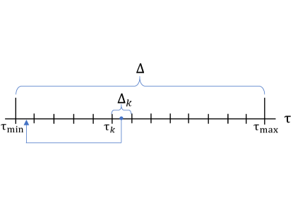
Figure 5: De-fading of data. See text for details

This problem is solved if Bob applies a classical Gaussian channel $y^{\prime k}\rightarrow y^{\prime\prime k}:=y^{\prime k}+\xi_{\text{add}}^{k}$ with additive noise $\mathrm{var}(\xi_{\text{add}}^{k})=(1-\tau_{\text{min}}/\tau_{k})\nu_{\text{det}}$. In this way, Bob generates

$$y^{\prime\prime k}=\sqrt{\tau_{\text{min}}}x+z^{\prime\prime k},$$ (122)

where $z^{\prime\prime k}$ is a Gaussian variable with variance

$$\sigma_{k}^{2}:=\mathrm{var}(z^{\prime\prime k})=2\bar{n}(\tau_{k})\tau_{\text{min}}/\tau_{k}+\nu_{\text{det}}\geq\nu_{\text{det}}.$$ (123)

We see that the transformation $y^{k}\rightarrow y^{\prime\prime k}$ is a slot-dependent beam-splitter channel $\mathcal{C}_{k}$ performed over the data, with transmissivity $\iota_{k}:=\tau_{\text{min}}/\tau_{k}$ and environmental noise-variance equal to $\nu_{\text{det}}$. Equivalently, this can be represented by a virtual beam splitter directly applied to the pulses allocated to slot $\Delta_{k}$ followed by the measurement. In other words, Alice and Bob’s input-output relation $x\rightarrow y^{\prime\prime k}$ is equivalent to the action of a composite Gaussian channel $\mathcal{F}_{k}:=\mathcal{C}_{k}\circ\mathcal{E}_{k}$, where $\mathcal{E}_{k}$ is a thermal-loss channel with transmissivity $\tau_{k}$ and thermal number $\bar{n}(\tau_{k})$, followed by Bob’s measurement.

Assuming that the transformation $y^{k}\rightarrow y^{\prime\prime k}$ is performed for all the $M$ slots of the interval, Bob creates a new variable $y^{\prime\prime}$ which satisfies

$$y^{\prime\prime}=\sqrt{\tau_{\text{min}}}x+z^{\prime\prime},$$ (124)

where $z^{\prime\prime}$ is non-Gaussian. Since $x\rightarrow y\rightarrow y^{\prime\prime}$ is a Markov chain, Bob’s post-processing can only decrease the mutual information $I(x:y^{\prime\prime})\leq I(x:y)$. The noise variable $z^{\prime\prime}$ can be written as an ensemble $\{\pi_{k},z^{\prime\prime k}\}$, with the independent element $z^{\prime\prime k}$ being selected with probability $\pi_{k}=p_{k}/p_{\Delta}$. Thus, it has zero mean and variance

$$\sigma_{z^{\prime\prime}}^{2}=\sum\limits_{k=1}^{M}\pi_{k}\sigma_{k}^{2}=\nu_{\text{det}}+2\tau_{\text{min}}\sum\limits_{k=1}^{M}\frac{\pi_{k}}{\tau_{k}}\bar{n}(\tau_{k}).$$ (125)

Overall, the transformation of Eq. (124) is equivalently obtained by measuring the output of a non-Gaussian channel $\mathcal{F}$, which is described by the ensemble $\{\pi_{k},\mathcal{F}_{k}\}$ and assumed to be completely controlled by Eve.

Due to the optimality of collective Gaussian attacks for Gaussian-modulated coherent-state protocols, the parties may assume the worst-case scenario where the non-Gaussian channel $\mathcal{F}$ is replaced by a thermal-loss Gaussian channel $\mathcal{E}_{\tau_{\text{min}},\bar{n}_{\text{G}}}$ with the same transmissivity $\tau_{\text{min}}$ and thermal number

$$\bar{n}_{\text{G}}=\tau_{\text{min}}\sum\limits_{k=1}^{M}\frac{\pi_{k}}{\tau_{k}}\bar{n}(\tau_{k}),$$ (126)

so that it has noise variance $\sigma_{\text{G}}^{2}=2\bar{n}_{\text{G}}+\nu_{\text{det}}$ equal to $\sigma_{z^{\prime\prime}}^{2}$ of Eq. (125). This means that the noise variable $z^{\prime\prime}$ in Eq. (124) can be replaced by a Gaussian variable $z_{\text{G}}$, and the total input-output relation is assumed to be

$$y^{\prime\prime}=\sqrt{\tau_{\text{min}}}x+z_{\text{G}}.$$ (127)

Thus, we lower-bound Alice and Bob’s performance by considering the post-processed variables $\{x,y^{\prime\prime}\}$ connected by the input-output relation of Eq. (127), after de-fading and assuming a Gaussian attack (‘Gaussianification’). This leads to the asymptotic key rate

$$R_{\text{asy}}=\beta I(x:y^{\prime\prime})_{\tau_{\text{min}},\bar{n}_{\text{G}}}-\chi(\mathbf{E}:y^{\prime\prime})_{\tau_{\text{min}},\bar{n}_{\text{G}}},$$ (128)

which can be computed from Eq. (73). The explicit expressions for the mutual information $I$ and the Holevo bound $\chi$ are given in Secs. III.1 and III.3, for the homodyne ($R_{\text{asy}}^{\text{hom}}$) and heterodyne protocol ($R_{\text{asy}}^{\text{het}}$) NoteBETA .

Because we have reduced the fading process to a stable thermal-loss channel $\mathcal{E}_{\tau_{\text{min}},\bar{n}_{\text{G}}}$, we can exploit the methodology of Sec. III. In particular, we can apply the tools of Sec. III.4 to compute the estimators/worst-case estimators for $\tau_{\text{min}}$ and $\bar{n}_{\text{G}}$, to be employed in the key rate.

IV.5 Estimating the channel parameters

In the parameter estimation step, Alice and Bob sacrifice some of their signals in order to estimate the actual values of the minimum transmissivity $\tau_{\min}=T_{\text{min}}^{2}$ and the Gaussian noise $\sigma_{\text{G}}^{2}$ (or $\bar{n}_{\text{G}}$) up to an acceptable error probability. Note that, in general, the actual value of $\tau_{\min}$ might be different from what determined via the pilots, so that its estimation via the signals is needed. In fact, Eve might try to use a QND measurement to distinguish between pilots and signals. After such QND measurement (with loss $\tau_{k}$), Eve may apply an additional measurement (with loss $\tilde{\tau}$) only to the signals. This means that, after de-fading, the input-output relation of Eq. (127) would become $\tilde{y}^{\prime\prime}=\sqrt{\tilde{\tau}_{\text{min}}}x+\tilde{z}_{\text{G}}$, with lower transmissivity $\tilde{\tau}_{\text{min}}:=\tilde{\tau}\tau_{\text{min}}$ and generally higher noise $\tilde{z}_{\text{G}}$.

Because parameter estimation is performed over a subset of the signals, the parties will detect these discrepancies with respect to the pilots. Most importantly, they will derive the corresponding estimators for the lower transmissivity $\tilde{\tau}_{\text{min}}$ and the different noise level, to be used in the calculation of their secret key. Of course, Eve might be more disruptive over the signals so that their transmissivity might be sensibly different from that of the corresponding pilots, but the point is that any such a perturbation will be anyway detected/estimated by the parties. If the discrepancy between pilots and signals is too strong, the noise level detected by the parties becomes too high for secure communication (denial of service). In the following, we make the realistic assumption that Eve acts universally over pilots and signals, so that $\tilde{\tau}_{\text{min}}=\tau_{\text{min}}$. However, we point out that this is only a simplification, not a limitation of the approach whose application to $\tilde{\tau}_{\text{min}}\neq\tau_{\text{min}}$ is immediate.

In order to create their estimators, the parties sacrifice $mp_{\Delta}$ signals from those they have post-selected. This corresponds to $m_{\Delta}:=\nu_{\text{det}}mp_{\Delta}$ pairs of data points $\{x,y^{\prime\prime}\}$, and we can also write $m_{\Delta}=\sum\nolimits_{k=1}^{M}m_{k}$, where $m_{k}:=\nu_{\text{det}}mp_{k}$ is the contribution coming from the generic slot $\Delta_{k}$. In writing $mp_{\Delta}$, we implicitly assume that $m$ is the equivalent number of signals that would have been sacrificed by the parties in the absence of post-selection. This notation is theoretical useful to describe scenarios where the same protocol (with fixed $m$) is implemented over different distances over which the value of $p_{\Delta}$ can be optimized.

For the square-root transmissivity, Alice and Bob build the estimator

$$\hat{T}_{\text{min}}:=\left.\sum\limits_{i=1}^{m_{\Delta}}x_{i}y_{i}^{\prime\prime}\right/\sum\limits_{i=1}^{m_{\Delta}}x_{i}^{2}\simeq\frac{1}{m_{\Delta}\sigma_{x}^{2}}\sum\limits_{i=1}^{m_{\Delta}}x_{i}y_{i}^{\prime\prime}.$$ (129)

It is easy to check that this is unbiased (i.e., its mean is $\simeq T_{\text{min}}$) and its variance is given by

$$\mathrm{var}(\hat{T}_{\text{min}}) \simeq\frac{1}{m_{\Delta}^{2}\sigma_{x}^{4}}\sum\limits_{i=1}^{m_{\Delta}}\mathrm{var}(x_{i}y_{i}^{\prime\prime})$$ (130)

$$=\frac{1}{m_{\Delta}^{2}\sigma_{x}^{4}}\sum\limits_{k=1}^{M}\sum\limits_{i_{k}=1}^{m_{k}}\mathrm{var}(x_{i_{k}}y_{i_{k}}^{\prime\prime k})$$ (131)

$$\simeq\frac{1}{m_{\Delta}^{2}\sigma_{x}^{4}}\sum\limits_{k=1}^{M}m_{k}\mathrm{var}(xy^{\prime\prime k})$$ (132)

$$=\frac{1}{m_{\Delta}^{2}\sigma_{x}^{4}}\sum\limits_{k=1}^{M}m_{k}(2\tau_{\text{min}}\sigma_{x}^{4}+\sigma_{x}^{2}\sigma_{k}^{2})$$ (133)

$$=\frac{1}{m_{\Delta}}\left(2\tau_{\text{min}}+\frac{1}{m_{\Delta}\sigma_{x}^{2}}\sum\limits_{k=1}^{M}m_{k}\sigma_{k}^{2}\right)$$ (134)

$$=\frac{2\tau_{\text{min}}+\sigma_{\text{G}}^{2}/\sigma_{x}^{2}}{m_{\Delta}}.$$ (135)

Let us build an estimator for the variance $\sigma_{\text{G}}^{2}$ of the thermal noise $z_{\text{G}}$. This is given by

$$\widehat{\sigma_{\text{G}}^{2}} :=\frac{1}{m_{\Delta}}\sum\limits_{i=1}^{m_{\Delta}}\left(y_{i}^{\prime\prime}-\hat{T}_{\text{min}}x_{i}\right)^{2}$$ (136)

$$\simeq\frac{1}{m_{\Delta}}\sum\limits_{k=1}^{M}\sum\limits_{i_{k}=1}^{m_{k}}\left(y_{i_{k}}^{\prime\prime k}-T_{\text{min}}x_{i_{k}}\right)^{2}$$ (137)

$$=\frac{1}{m_{\Delta}}\sum\limits_{k=1}^{M}\sigma_{k}^{2}Y_{k},~{}~{}Y_{k}:=\sum\limits_{i_{k}=1}^{m_{k}}\frac{(z_{i_{k}}^{\prime\prime k})^{2}}{\sigma_{k}^{2}},$$ (138)

where $Y_{k}$ is distributed according to a $\chi^{2}$ distribution with $m_{k}$ degrees of freedom. It is easy to check that the estimator is unbiased, i.e., we have

$$\langle\widehat{\sigma_{\text{G}}^{2}}\rangle=\frac{1}{m_{\Delta}}\sum\limits_{k=1}^{M}\sigma_{k}^{2}\langle Y_{k}\rangle\simeq\sigma_{\text{G}}^{2}.$$ (139)

Then, for the variance we compute

$$\mathrm{var}(\widehat{\sigma_{\text{G}}^{2}})=\frac{1}{m_{\Delta}^{2}}\sum\limits_{k=1}^{M}\sigma_{k}^{4}\mathrm{var}(Y_{k})\simeq\frac{2}{m_{\Delta}^{2}}\sum\limits_{k=1}^{M}m_{k}\sigma_{k}^{4}.$$ (140)

Equivalently, in terms of number of thermal photons $\bar{n}_{\text{G}}:=(\sigma_{\text{G}}^{2}-\nu_{\text{det}})/2$, we write the estimator

$$\widehat{\bar{n}_{\text{G}}}:=(\widehat{\sigma_{\text{G}}^{2}}-\nu_{\text{det}})/2,$$ (141)

which is unbiased $\langle\widehat{\bar{n}_{\text{G}}}\rangle\simeq\bar{n}_{\text{G}}$ with $\mathrm{var}(\widehat{\bar{n}_{\text{G}}})=\mathrm{var}(\widehat{\sigma_{\text{G}}^{2}})/4$.

It is important to note that all the mean values and variances above are computable by the parties by replacing estimators in the right-hand sides of the formulas. In fact, once $\hat{T}_{\text{min}}$ and $\widehat{\sigma_{\text{G}}^{2}}$ have been computed, these can be replaced in Eq. (135) to provide $\mathrm{var}(\hat{T}_{\text{min}})$. To compute $\mathrm{var}(\widehat{\sigma_{\text{G}}^{2}})$, the parties need to derive estimators of $\sigma_{k}^{2}$, i.e.,

$$\widehat{\sigma_{k}^{2}}:=\frac{1}{m_{k}}\sum\limits_{i_{k}=1}^{m_{k}}\left(y_{i_{k}}^{\prime\prime k}-\hat{T}_{\text{min}}x_{i_{k}}\right)^{2},$$ (142)

whose squares go in Eq. (140).

IV.6 Worst-case estimators and bounds

According to Eq. (127), Alice and Bob’s post-processed data is generated by a thermal-loss channel $\mathcal{E}_{\tau_{\text{min}},\bar{n}_{\text{G}}}$ with transmissivity $\tau_{\text{min}}$ and thermal number $\bar{n}_{\text{G}}$. For the transmissivity and the thermal number, we write the worst-case estimators

$$\tau_{\text{min}}^{\prime} :=\left[\hat{T}_{\text{min}}-w~{}\sqrt{\mathrm{var}(\hat{T}_{\text{min}})}\right]^{2}$$

$$\simeq\hat{T}_{\text{min}}^{2}-2w\hat{T}_{\text{min}}\sqrt{\mathrm{var}(\hat{T}_{\text{min}})}+\mathcal{O}(m_{\Delta}^{-1}),$$ (143)

$$\bar{n}_{\text{G}}^{\prime} :=\widehat{\bar{n}_{\text{G}}}+w~{}\sqrt{\mathrm{var}(\widehat{\bar{n}_{\text{G}}})},$$ (144)

where the confidence parameter $w$ is connected to the error $\varepsilon_{\text{pe}}$ according to Eq. (87) or Eq. (96).

For the sake of the theoretical analysis, it is useful to introduce bounds for $\tau_{\text{min}}^{\prime}$ and $\bar{n}_{\text{G}}^{\prime}$. Consider the worst-case noise variance $\sigma_{\text{wc}}^{2}=2\bar{n}_{\text{wc}}+\nu_{\text{det}}$ such that $\sigma_{\text{wc}}^{2}\geq\sigma_{k}^{2}$ for any slot $k$. Then, we may write

$$\mathrm{var}(\hat{T}_{\text{min}}) \lesssim\frac{2\tau_{\text{min}}+\sigma_{\text{wc}}^{2}/\sigma_{x}^{2}}{m_{\Delta}},$$ (145)

$$\langle\widehat{\bar{n}_{\text{G}}}\rangle \lesssim\bar{n}_{\text{wc}},~{}\mathrm{var}(\widehat{\bar{n}_{\text{G}}})\lesssim\frac{(2\bar{n}_{\text{wc}}+\nu_{\text{det}})^{2}}{2m_{\Delta}}.$$ (146)

As a result, we have the bounds

$$\tau_{\text{min}}^{\prime} \gtrsim\tau_{\text{LB}}:=\tau_{\text{min}}-2w\sqrt{\frac{2\tau_{\text{min}}^{2}+\tau_{\text{min}}\sigma_{\text{wc}}^{2}/\sigma_{x}^{2}}{m_{\Delta}}},$$ (147)

$$\bar{n}_{\text{G}}^{\prime} \lesssim\bar{n}_{\text{UB}}:=\bar{n}_{\text{wc}}+w\frac{2\bar{n}_{\text{wc}}+\nu_{\text{det}}}{\sqrt{2m_{\Delta}}}.$$ (148)

Let us now evaluate the worst-case thermal number $\bar{n}_{\text{wc}}$ to be used in the bounds above. We write

$$\bar{n}_{\text{wc}}=\eta_{\text{eff}}\bar{n}_{B}+\bar{n}_{\text{ex,wc}},$$ (149)

where $\bar{n}_{\text{ex,wc}}:=\bar{n}_{\text{ex}}(\tau_{\text{wc}})\geq\bar{n}_{\text{ex}}(\tau)$ is computed over the worst-case value$\ \tau_{\text{wc}}$. The latter may be chosen to be$\ \tau_{\text{wc}}=\tau_{\text{min}}$ for the TLO and $\tau_{\text{wc}}=\tau_{\text{max}}$ for the LLO [due to the fact that $\bar{n}_{\text{ex}}(\tau)$ has different monotonicity in $\tau$, as discussed in Sec. III.2.3]. In other words, for $\bar{n}_{\text{ex,wc}}$, we may consider the two estimates

$$\bar{n}_{\text{ex,wc}}^{\text{TLO}} \simeq\Theta_{\text{el}}/\tau_{\text{min}},$$ (150)

$$\bar{n}_{\text{ex,wc}}^{\text{LLO}} \simeq\Theta_{\text{el}}+\pi\tau_{\text{max}}\sigma_{x}^{2}C^{-1}l_{\text{W}},$$ (151)

where $\Theta_{\text{el}}$ is the electronic noise term in Eq. (61).

In our numerical investigations, we assume the bounds $\tau_{\text{LB}}$ and $\bar{n}_{\text{UB}}$ in Eqs. (147) and (148), which take different expressions for TLO and LLO depending on Eqs. (150) and (151). Since each of these worst-case estimators is correct up to an error $\varepsilon_{\text{pe}}$, the total error affecting the procedure of parameter estimation is $\simeq 2\varepsilon_{\text{pe}}$.

IV.7 Composable key rate for free-space CV-QKD

Let us summarize the scenario. Alice and Bob perform a Gaussian-modulated coherent-state (homodyne or heterodyne) protocol with variance $\sigma_{x}^{2}=\mu-1$ over a free-space channel with instantaneous transmissivity $\eta_{\text{ch}}$ and background thermal noise $\bar{n}_{B}$. The receiver has setup efficiency $\eta_{\text{eff}}$ and setup noise $\bar{n}_{\text{ex}}$, so that the total thermal noise is $\bar{n}=\eta_{\text{eff}}\bar{n}_{B}+\bar{n}_{\text{ex}}$. The overall instantaneous transmissivity from Alice to Bob is given by $\tau=\eta_{\text{ch}}\eta_{\text{eff}}$ and it fluctuates following a fading distribution $P_{0}(\tau)$ as in Eq. (25). Because $\bar{n}_{\text{ex}}=\bar{n}_{\text{ex}}(\tau)$ [see Sec. III.2.3], we also have thermal-noise fluctuations $\bar{n}=\bar{n}(\tau)$. The physical scenario is depicted in Fig. 1, and also modelled in Fig. 4 for each fixed value of the transmissivity.

Alice sends to Bob a total of $N$ pulses which are multiplexed with an LO in polarization (TLO) or in time (LLO). Note that in terms of throughput (bits/sec), given by the rate (bits/use) times the clock $C$ (uses/sec), one should account for the additional uses of the link associated with the LO. Thus, there is a factor of $1/2\$for the LLO, unless this is compensated by using two polarizations for the quantum signals (see Sec. III.2.1).

Within the total set of $N$ pulses, there are $m_{\text{P}}$ pilots that are prepared in a bright coherent state and are randomly interleaved with the $N-m_{\text{P}}$ signal pulses. Thanks to these pilots, the parties monitor the instantaneous transmissivity $\tau$ and they create a post-selection interval $\Delta:=[\tau_{\min},\tau_{\max}]$, where $\tau_{\text{max}}=\eta:=\eta_{\text{st}}\eta_{\text{atm}}\eta_{\text{eff}}$ is the maximum value achievable and $\tau_{\text{min}}=f_{\text{th}}\eta$ for some threshold value $f_{\text{th}}\in(0,1)$. The interval $\Delta$ post-selects a portion $S_{\Delta}=(N-m_{\text{P}})p_{\Delta}$ of the signals, where the probability $p_{\Delta}=p(\tau_{\text{min}},\tau_{\text{max}})$ is given in Eq. (115). Then, the interval is further divided into a lattice of $M$ slots with small step $\delta\tau$, so that each slot $\Delta_{k}:=[\tau_{k},\tau_{k+1}]$ collects signals with almost-equal transmissivity $\tau\simeq\tau_{k}:=\tau_{\text{min}}+(k-1)\delta\tau$.

The post-selected $S_{\Delta}$ signals provide $\nu_{\text{det}}S_{\Delta}$ pairs of data points $\{x_{i},y_{i}\}$ where $x$ is Alice’s generic quadrature encoding and $y$ is Bob’s corresponding decoding. The outcomes $\{y_{i}\}$ are all mapped into the first slot $\Delta_{1}$ with minimum transmissivity $\tau_{\text{min}}$, by means of the de-fading channel $y\rightarrow$ $y^{\prime\prime}$ described in Sec. IV.4. As a result, Alice and Bob’s data points satisfy the input-output relation $y^{\prime\prime}=\sqrt{\tau_{\text{min}}}x+z_{\text{G}}$ of Eq. (127), which is equivalent to a thermal-loss channel $\mathcal{E}_{\tau_{\text{min}},\bar{n}_{\text{G}}}$ with transmissivity $\tau_{\text{min}}$ and thermal number $\bar{n}_{\text{G}}$, so that $\sigma_{\text{G}}^{2}=2\bar{n}_{\text{G}}+\nu_{\text{det}}$.

Alice and Bob sacrifice $mp_{\Delta}$ signals to derive worst-case estimators $\tau_{\text{min}}^{\prime}$ and $\bar{n}_{\text{G}}^{\prime}$ according to Eqs. (143) and (144), where the confidence parameter $w$ is determined by the error $\varepsilon_{\text{pe}}$ according to Eq. (87) or Eq. (96). These estimators are used to compute the asymptotic key rate affected by parameter estimation

$$R_{\text{pe}}=R_{\text{asy}}(\tau_{\text{min}}^{\prime},\bar{n}_{\text{G}}^{\prime}),$$ (152)

where $R_{\text{asy}}$ is given in Eq. (128). For the theoretical analysis, we consider the further lower bound

$$R_{\text{pe}}\geq R_{\text{LB}}:=R_{\text{asy}}(\tau_{\text{LB}},\bar{n}_{\text{UB}}),$$ (153)

which is based on $\tau_{\text{LB}}$ and $\bar{n}_{\text{UB}}$ from Eqs. (147) and (148).

The signals remaining for key generation are $np_{\Delta}$, where $n=N-(m+m_{\text{P}})$. Thus, after parameter estimation, the parties process their $np_{\Delta}\nu_{\text{det}}$ key generation points $\{x_{i},y_{i}^{\prime\prime}\}$ via the procedures of error correction and privacy amplification. Depending on the reconciliation parameter $\beta$ (related to the rate of the error-correcting code) and the correctness $\varepsilon_{\text{cor}}$ (related to the probability of residual errors in Alice’s and Bob’s corrected strings), the step of error correction has an associated success probability $p_{\text{ec}}$ to promote the block of points to the next step of privacy amplification. The latter procedure is ideal (i.e., decouples Eve) up to an error quantified by the secrecy parameter $\varepsilon_{\text{sec}}=\varepsilon_{\text{s}}+\varepsilon_{\text{h}}$, in turn decomposed into a smoothing ($\varepsilon_{\text{s}}$) and a hashing parameter ($\varepsilon_{\text{h}}$). After privacy amplification, an average number of $np_{\Delta}p_{\text{ec}}$ signals contribute to the final key, leading to an overall factor $np_{\Delta}p_{\text{ec}}/N$ in front of the rate.

The composable finite-size key rate associated with the post-selection interval $\Delta$ is bounded by

$$R\geq\frac{np_{\Delta}p_{\text{ec}}}{N}\left(R_{\text{LB}}-\frac{\Delta_{\text{aep}}}{\sqrt{np_{\Delta}}}+\frac{\Theta}{np_{\Delta}}\right),$$ (154)

where the two terms $\Delta_{\text{aep}}$ and $\Theta$ are given in Eqs. (106) and (107) for some value $\log_{2}d$ of digitalization. This rate is $\varepsilon$-secure against collective Gaussian attacks, where $\varepsilon=2p_{\text{ec}}\varepsilon_{\text{pe}}+\varepsilon_{\text{cor}}+\varepsilon_{\text{sec}}$. The expression of the key rate in Eq. (154) can be specified for the homodyne/heterodyne protocol and for the two types of LO (TLO/LLO).

For the heterodyne protocol, we can extend the key rate to composable finite-size security against general coherent attacks (see Sec. III.6). This is done by adopting a suitable symmetrization and including energy tests, both operations to be performed on the data points $\{x_{i},y_{i}^{\prime\prime}\}$. The number of energy tests is set to be $p_{\Delta}m_{\mathrm{et}}$, where $m_{\mathrm{et}}=f_{\mathrm{et}}n$ for some factor $f_{\mathrm{et}}<1$. Thus, the final key generation signals will be $np_{\Delta}p_{\text{ec}}$ with

$$n=N-(m+m_{\text{P}}+m_{\text{et}})=\frac{N-(m+m_{\text{P}})}{1+f_{\mathrm{et}}}.$$ (155)

The composable key rate is bounded as follows

$$R_{\text{gen}}^{\text{het}}\geq\frac{np_{\Delta}p_{\text{ec}}}{N}\left(R_{\text{LB}}^{\text{het}}-\frac{\Delta_{\text{aep}}}{\sqrt{np_{\Delta}}}+\frac{\Theta-\Phi_{np_{\Delta}}}{np_{\Delta}}\right),$$ (156)

where the extra term $\Phi_{n}$ is defined as in Eq. (110) and is expressed in terms of $K_{n}$ of Eq. (111), for which we choose the dimensions $d_{R}=d_{T}\simeq\bar{n}_{T}=\sigma_{x}^{2}/2$ (so that the energy test succeeds with probability $p_{\text{et}}\simeq 1$).

Note that the key rate $R_{\text{gen}}^{\text{het}}$ is secure up to an epsilon security $\varepsilon^{\prime}=K_{np_{\Delta}}^{4}\varepsilon/50$. This means that, in order to get $\varepsilon^{\prime}\simeq 10^{-10}$ against general attacks, we need to start from a security of $\varepsilon\simeq 10^{-43}$ against collective Gaussian attacks. In turn, this also implies $\varepsilon_{\text{pe}}\simeq 10^{-43}$, so we need to use Eq. (96) for the worst-case estimators.

IV.8 Numerical simulations

In our numerical investigations we consider the heterodyne protocol, for which we study the free-space composable key rate under collective and coherent attacks, assuming the two types of LO. The free-space model is the same as in Sec. II and depicted in Fig. 1. We consider the $z$-propagation of a collimated Gaussian beam which is subject to diffraction, atmospheric extinction $\eta_{\text{atm}}$ [as quantified by the Beer-Lambert equation of Eq. (5)], pointing error $\sigma_{\text{P}}^{2}\simeq(10^{-6}z)^{2}$ (for an error of $1~{}\mu$rad at the transmitter), and Rytov-Yura weak turbulence ($\sigma_{\text{Rytov}}^{2}<1$) under the Hufnagel-Valley model of atmosphere (see Appendix C). Turbulence leads to beam broadening, with short-term transmissivity $\eta_{\text{st}}$, and centroid wandering, with variance $\sigma_{\text{TB}}^{2}$. Including the setup efficiency $\eta_{\text{eff}}$, we have a maximum transmissivity $\eta:=\eta_{\text{st}}\eta_{\text{atm}}\eta_{\text{eff}}$ when the beam is perfectly-aligned. The overall wandering, with variance $\sigma^{2}=\sigma_{\text{P}}^{2}+\sigma_{\text{TB}}^{2}$, leads to the distribution $P_{0}(\tau)$ of Eq. (25) for the instantaneous transmissivity $\tau$ of the link. Thermal background follows the description of Sec. II.4 for cloudy day-time conditions (but suppressed by the homodyne filter). In particular, we assume the physical parameters listed in Table 1.

Physical parameter	Symbol	Value
Beam curvature	$R_{0}$	$\infty$
Wavelength	$\lambda$	$800~{}$nm
Beam spot size	$w_{0}$	$5~{}$cm
Receiver aperture	$a_{R}$	$5~{}$cm
Receiver field of view	$\Omega_{\text{fov}}$	$10^{-10}~{}$sr
Homodyne filter	$\Delta\lambda$	$0.1~{}\text{pm}$
Detector efficiency	$\eta_{\text{eff}}$	$0.5$
Detector bandwidth	$W$	$100~{}$MHz
Noise equivalent power	NEP	$6~{}$pW/$\sqrt{\text{Hz}}$
Linewidth	$l_{\text{W}}$	$1.6$ KHz
LO power	$P_{\text{LO}}$	$100~{}$mW
Clock	$C$	$5~{}$MHz
Pulse duration	$\Delta t,\Delta t_{\text{LO}}$	$10~{}$ns
Altitude	$h$	$30~{}$m
Structure constant (day)	$C_{n}^{2}$	$2.06\times 10^{-14}~{}$m-2/3
$\begin{array}[c]{l}\text{Background noise}\\ \text{(day, }\Delta\lambda=0.1~{}\text{pm)}\end{array}$	$\bar{n}_{B}$	$4.75\times 10^{-7}$

Table 1: Physical parameters.

The steps of the protocol are those explained in the previous subsection, where Alice and Bob assume a post-selection interval $\Delta:=[\tau_{\min},\tau_{\max}]$ with $\tau_{\text{max}}=\eta$ and $\tau_{\text{min}}=f_{\text{th}}\eta$ for some threshold value $f_{\text{th}}\in(0,1)$. In particular, we choose the parameters listed in Table 2.

$\begin{array}[c]{l}\text{Protocol}\\ \text{parameter}\end{array}$	Symbol	$\begin{array}[c]{l}\text{Collective}\\ \text{attacks}\end{array}$	$\begin{array}[c]{l}\text{General}\\ \text{attacks}\end{array}$
Total pulses	$N$	$5\times 10^{7}$	$5\times 10^{7}$
Pilot pulses	$m_{\text{P}}$	$0.1\times N$	$0.1\times N$
PE signals	$m$	$0.1\times N$	$0.1\times N$
Energy tests	$f_{\text{et}}$	$-$	$0.2$
KG signals	$n$	$0.8\times N$	$\simeq 3.33\times 10^{7}$
Digitalization	$d$	$2^{5}$	$2^{5}$
Rec. efficiency	$\beta$	$0.98$	$0.98$
EC success prob	$p_{\text{ec}}$	$0.9$	$0.5$
Epsilons	$\varepsilon_{\text{h,s,\ldots}}$	$2^{-33}\simeq 10^{-10}$	$10^{-43}$
Confidence	$w$	$\simeq 6.34$	$\simeq 14.07$
Security	$\varepsilon,\varepsilon^{\prime}$	$\simeq 5.6\times 10^{-10}$	$\lesssim 1.3\times 10^{-9}$
Modulation	$\mu$	variable	$\begin{array}[c]{l}20~{}\text{(TLO)}\\ 8.4~{}\text{(LLO)}\end{array}$
Threshold	$f_{\text{th}}~{}$	variable	$0.84$

Table 2: Protocol parameters.

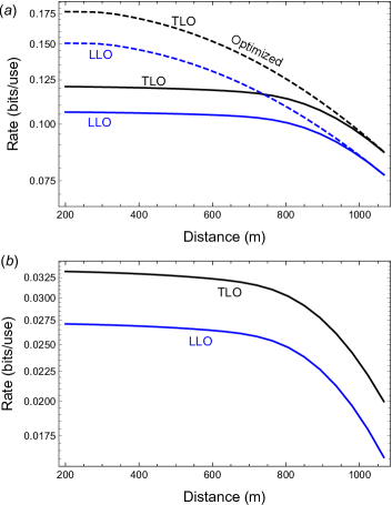
Figure 6: Composable secret-key rates (bits/use) versus distance (m) for free-space QKD in the regime of weak turbulence and for cloudy day-time operation. We consider a coherent-state protocol with heterodyne detection, pilot-guided and operated in post-selection as described in the main text. Physical and protocol parameters are listed in Tables 1 and 2. (a) We plot the secret key rate of Eq. (154) assuming a TLO (black curves) and an LLO (blue curves). In particular, we plot the performances at fixed post-selection threshold $f_{\text{th}}=0.84$ and fixed input modulation, $\mu=20$ for TLO and $\mu=8.4$ for LLO (solid curves). These are chosen to optimize the rates at the maximum distance ($z=1066~{}$m). We compare these performances with those achievable by optimizing the rates over $\mu$ and $f_{\text{th}}$ at each distance (dashed curves). (b) We plot the rate of Eq. (156) against general attacks for TLO (black line) and LLO (blue line). These performances are not optimized and refer to fixed threshold $f_{\text{th}}=0.84$ and input modulation ($\mu=20$ for TLO and $\mu=8.4$ for LLO).

As we can see from Fig. 6(a), the composable key rates against collective attacks are sufficiently high, even though these values actually represent lower bounds to what achievable by Alice and Bob. As a matter of fact, in most of the weak-turbulence range, these rates are within one order of magnitude of the ultimate loss-based upper bound of Eq. (27) which is plotted as red dashed line in Fig. 2(a), computed for day-time and the same physical parameters considered here. In Fig. 6(a), we study the rates that are achievable with the TLO and the LLO. In one setting (solid curves), we fix the value of the threshold parameter for post-selection $f_{\text{th}}$ to $84\%$ and we also fix the value of the input Gaussian modulation ($\mu=20$ for TLO and $\mu=8.4$ for LLO). These values are chosen to maximize the rates at the maximum distance $z=1066~{}$m, but they are not the optimal choices for the other distances. In another approach, we maximize the rates over $f_{\text{th}}$ and $\mu$ at each distance, finding substantially improved performances (dashed lines).

In Fig. 6(b), we plot the composable key rates achievable against general attacks assuming no optimization in $f_{\text{th}}$ and $\mu$. On the one hand, these rates are not far from the corresponding results against collective attacks. On the other hand, the choice of parameters in Table 2 may be far more challenging for this general case (e.g., in terms of $\beta$ and $p_{\text{ec}}$ for such a low value of $\varepsilon_{\text{cor}}$). Also note that the final epsilon security $\varepsilon^{\prime}$ depends on the distance. For the parameters chosen, this ranges from $\simeq 1.38\times 10^{-11}$ for the LLO at $z=1066~{}$m and $\simeq 1.32\times 10^{-9}$ for the TLO at $z=200~{}$m.

A final important observation (already mentioned before but here relevant to stress) is that the rates shown in Fig. 6 refer to bits per use of the quantum communication channel, without accounting for the transmission of the LO-reference pulses. If we include the clock of the system (uses/second) and compute the throughput of the communication (bits/second), then we need to include the uses of the link dedicated to the LO. Thus, for the LLO, we should halve the final rate (with respect to the TLO) due to the time multiplexing of the LO. However, it is also true that, with the LLO, one could use both polarizations in the transmission of the signals, so that the factor $1/2$ in the final rate can be fully compensated.

V Conclusions

In conclusion, we have established the ultimate bounds for free-space quantum communications under general conditions of diffraction, atmospheric extinction, pointing errors, turbulence, and background thermal noise. We have first developed the theory for the regime of weak turbulence, crucial for free space ground-communications in a relatively short range, and then extended the results to the case of stronger turbulence. In the short range, we have then derived achievable and composable key rates for free-space CV-QKD, proving that these rates are sufficiently close to the ultimate limits. This shows the robustness and suitability of free-space channels for implementing high-rate quantum-secured communications.

The achievable rates are derived by first formulating a general theory of composable finite-size security for Gaussian-modulated coherent-state protocols under conditions of channel stability, and then extending this theory to considering fading (non Gaussian) channels, which can be dealt via the introduction of pilot modes and suitable post-processing techniques. In this way we have been able to handle the difficult step of parameter estimation and to reduce the problem to the easier framework of a stable Gaussian channel. Fully assessing the practical security of CV-QKD in strong turbulent channels is an interesting future direction of investigation.

In conclusion our work not only established the ultimate limits and benchmarks for free-space quantum communications but also provided a comprehensive machinery for studying the composable finite-size security of CV-QKD protocols both in stable conditions (e.g., in standard fiber-based connections) and unstable conditions (i.e., in free-space links subject to fading effects).

Acknowledgements.– The author acknowledges funding from the European Union’s Horizon 2020 research and innovation programme under grant agreement No 820466 (Quantum-Flagship Project CiViQ: “Continuous Variable Quantum Communications”).

Appendix A Propagation of Gaussian beams

Most of the contents of this Appendix are basic notions of quantum optics. They are given here to set the general notation of the work and for the sake of completeness.

A.1 Free-space diffraction

Consider an optical bosonic mode with wavelength $\lambda$, angular frequency $\omega=2\pi c/\lambda$, and wavenumber $k=\omega/c=2\pi/\lambda$. Under the scalar approximation (single and uniform polarization) and the paraxial wave approximation, the electric field takes the form

$$E(x,y,z,t)=u(x,y,z)\exp[i(kz-\omega t)],$$ (157)

where the field amplitude $u(x,y,z)$ is a slowly varying function in the longitudinal propagation direction $z$, with $x$ and $y$ being the transverse coordinates and $t$ the time coordinate. The possible expressions for the field amplitude $u$ must satisfy the Fresnel-Kirchoff integral in the Fresnel approximation (svelto, , Eq. (4.6.9)). A solution of this integral which maintains its functional form, i.e., an eigensolution, is the Gaussian beam.

In particular, assume free-space propagation along the $z$ direction with no limiting apertures in the transverse plane, for which we introduce the radial coordinate $r=\sqrt{x^{2}+y^{2}}$. Then, the lowest order ($\mathrm{TEM}_{00}$) single-mode Gaussian beam takes a simple analytical expression. At the initial position $z=0$, its field amplitude has the form

$$u(0,r)=\exp(-r^{2}/w_{0}^{2})\exp{[-ikr^{2}/(2R_{0})]},$$ (158)

where $w_{0}$ is the beam spot size and $R_{0}$ is the phase-front radius of curvature. For beam spot size we precisely mean the ‘field’ spot size, corresponding to the radial distance at which the amplitude of the field decays to $1/e$ of its maximum value. Note that the intensity of the beam is given by $I(0,r)=\exp\left(-2r^{2}/w_{0}^{2}\right)$, so that one can define an ‘intensity’ spot size $w_{0}^{\text{I}}=w_{0}/\sqrt{2}$, that is also widely used in the literature (e.g., in Refs. Yura73 ; Fante75 ).

Let us introduce the ‘Rayleigh range’

$$z_{R}:=\frac{\pi w_{0}^{2}}{\lambda},$$ (159)

and the Fresnel number of the beam

$$f:=\frac{\pi w_{0}^{2}}{\lambda z}=\frac{z_{R}}{z},$$ (160)

so that the far-field regime ($z\gg z_{R}$) corresponds to $f\ll 1$. Following the notation of Ref. Andrews93 , we also introduce the Fresnel ratio $\Omega:=f^{-1}$ and the curvature parameter $\Omega_{0}:=1-z/R_{0}$. Note that a collimated beam ($R_{0}=+\infty$) corresponds to $\Omega_{0}=1$, while a convergent beam ($R_{0}>0$) to $\Omega_{0}<1$, and a divergent beam ($R_{0}<0$) to $\Omega_{0}>1$.

In terms of the previous parameters, we can write the field at any distance $z$ as Andrews93 ; Andrews94

$$u(z,r)=\frac{w_{0}}{w_{z}}\exp(-r^{2}/w_{z}^{2})\exp{[-ikr^{2}/(2R_{z})-i\phi_{z}]},$$ (161)

where $\omega_{z}$ is the spot size at position $z$, $R_{z}$ is the corresponding curvature at $z$, and $\phi_{z}$ is its longitudinal phase at $z$, also known as Guoy phase shift (Siegman, , Sec. 17.4). These quantities take the following expressions

$$w_{z}^{2} =w_{0}^{2}\left(\Omega_{0}^{2}+\Omega^{2}\right),$$ (162)

$${R_{z}} {=}\frac{z(\Omega_{0}^{2}+\Omega^{2})}{\Omega_{0}(1-\Omega_{0})-\Omega^{2}},$$ (163)

$$\phi_{z} =\tan^{-1}(\Omega/\Omega_{0}).$$ (164)

More explicitly, we may write

$$w_{z}^{2} =w_{0}^{2}\left[\left(1-\frac{z}{R_{0}}\right)^{2}+\left(\frac{z}{z_{R}}\right)^{2}\right]$$ (165)

$$=w_{0}^{2}\left(1-\frac{z}{R_{0}}\right)^{2}+\frac{\lambda^{2}z^{2}}{\pi^{2}w_{0}^{2}}.$$ (166)

A typical assumption is to adopt the planar approximation of a collimated beam at the transmitter ($\Omega_{0}=1$). In such a case, it is immediate to check that

$$w_{z}^{2} =w_{0}^{2}[1+(z/z_{R})^{2}],$$ (167)

$$R_{z} =-z[1+(z_{R}/z)^{2}],$$ (168)

$$\phi_{z} =\tan^{-1}(z/z_{R}).$$ (169)

Note that $w_{z}^{2}$ is the sum of the initial (minimum) condition $w_{0}^{2}$ and a term $w_{0}^{2}(z/z_{R})^{2}$ which is due to diffraction. In the far-field, the latter term is dominant and we have

$$w_{z}\simeq w_{0}(z/z_{R})=\frac{\lambda z}{\pi w_{0}},$$ (170)

which increases linearly with the distance $z$. Defining beam divergence as $\theta:=w_{z}/z$, we write $\theta\simeq\lambda/(\pi w_{0})$, which increases with the wavelength (as expected). For a collimated beam, the curvature is minimal at $z=z_{R}$ and then goes as $\simeq z$ at large distance, so that the beam asymptotically becomes a spherical wave.

From Eq. (161), we see that the beam intensity at longitudinal distance $z$ is given by

$$I(z,r)=I_{\max}^{z}\exp\left(-2r^{2}/w_{z}^{2}\right),~{}I_{\max}^{z}:=w_{0}^{2}/w_{z}^{2}.$$ (171)

Assume that the beam is orthogonally intercepted by a receiver, which is described as a sharped-edged circular aperture with radial size $a_{R}$, therefore with total detection area $\pi a_{R}^{2}$. Let us compute the total power impinging on the finite-size detector by integrating over the radial coordinates $0\leq r\leq a_{R}$ and $0\leq\varphi\leq 2\pi$. We easily find

$$P(z,a_{R}) :={\displaystyle\int\limits_{0}^{2\pi}}d\varphi{\displaystyle\int\limits_{0}^{a_{R}}}rdrI(z,r)$$

$$=P_{z}\left(1-e^{-2a_{R}^{2}/w_{z}^{2}}\right),$$ (172)

where $P_{z}:=(\pi w_{z}^{2}I_{\max}^{z})/2$ represents the total power in the optical beam at distance $z$ (corresponding to a receiver of infinite radius $a_{R}\rightarrow\infty$). Note that we may also rewrite Eq. (171) as

$$I(z,r)=(2P_{z}/\pi w_{z}^{2})\exp(-2r^{2}/w_{z}^{2}).$$ (173)

The diffraction-limited transmissivity $\eta_{\text{d}}$ associated with the finite size of the receiver is given by

$$\eta_{\text{d}}:=P(z,a_{R})/P_{z}=1-e^{-2a_{R}^{2}/w_{z}^{2}},$$ (174)

where we may explicitly express $w_{z}^{2}$ as in Eq. (165). In the far field, we have $\Omega\gg 1$ in Eq. (162), so that$\ w_{z}\gg w_{0}$. Assuming that the receiver’s aperture radius $a_{R}$ is comparable to the spot size $w_{0}$, then we have $w_{z}\gg a_{R}$ and we can expand Eq. (174) into

$$\eta_{\text{d}}\simeq\eta_{\text{d}}^{\text{far}}:=\frac{2a_{R}^{2}}{w_{z}^{2}}\ll 1.$$ (175)

In particular, for a collimated beam we can use the approximation in Eq. (170) and write the far-field expression

$$\eta_{\text{d}}\simeq\eta_{\text{d}}^{\text{far,coll}}:=2\left(\frac{\pi w_{0}a_{R}}{\lambda z}\right)^{2}.$$ (176)

Recognizing that $A_{0}=\pi w_{0}^{2}$ and $A_{R}=\pi a_{R}^{2}$ as the effective transversal areas of the beam and the receiver’s aperture, we note that we may write Eq. (176) as $\eta_{\text{d}}\simeq 2f_{0R}$ where

$$f_{0R}:=A_{0}A_{R}/(\lambda z)^{2}$$ (177)

is the Fresnel number product associated with the beam and the receiver.

A.2 Diffraction at the transmitter

Any realistic transmitter involves an aperture with finite radius $a_{T}$. This means that the Gaussian profile of the beam could be truncated outside that radius causing diffraction. However, if the aperture $a_{T}$ is sufficiently larger than $w_{0}$, diffraction becomes negligible.

Assume that the transmitter has a plane exit pupil $\mathcal{A}_{0}$ of area $A_{0}$ while the receiver has an entrance pupil $\mathcal{A}_{z}$ of area $A_{z}$. We consider the quasi-monochromatic approximation where the transmitter excites planar modes within a narrow band of frequencies, centered around the carrier (angular) frequency $\omega$, and the receiver only detects planar modes within this bandwidth. We then consider the usual scalar approximation (i.e., a single and uniform polarization) and the paraxial wave approximation (so that the transverse components of the wave-vector are negligible at the receiver).

Let us write $\mathbf{x}:=(x,y)\in\mathcal{A}_{0}$ to be the transverse coordinates at the transmitter and $\mathbf{x}^{\prime}:=(x^{\prime},y^{\prime})\in\mathcal{A}_{z}$ those at the receiver. The electric field at the transmitter can then be expressed as Jeff

$$E_{0}(\mathbf{x},t)={\displaystyle\sum\limits_{k,l}}\hat{a}_{k,l}\Phi_{k}(\mathbf{x})\Psi_{l}(t),$$ (178)

where $\Phi_{k}(\mathbf{x})\Psi_{l}(t)$ are orthonormal spatiotemporal modes defined over $\mathcal{A}_{0}$ and $0\leq t\leq t_{\text{max}}$, with $t_{\text{max}}$ being the time duration of the transmitter’s signal. These modes have corresponding annihilation operators $\hat{a}_{k,l}$. Thanks to this normal-mode decomposition, one can express the electric field at the receiver, which is given by Jeff

$$E_{z}(\mathbf{x}^{\prime},t) ={\displaystyle\sum\limits_{k,l}}\left(\sqrt{\eta_{k}}\hat{a}_{k,l}+\sqrt{1-\eta_{k}}\hat{e}_{k,l}\right)$$

$$\times\Phi_{k}(\mathbf{x}^{\prime})\Psi_{l}(t-c^{-1}z),$$ (179)

for modes defined over $\mathcal{A}_{z}$ and $0\leq t-c^{-1}z\leq t_{\text{max}}$. Above, $\hat{e}_{k,l}$ are the annihilation operators associated with environmental modes impinging on the pupil of the receiver, which are generally described by thermal states.

Free-space diffraction-limited quantum communication can therefore be completed described by the input-output relations

$$\hat{a}_{k,l}\rightarrow\hat{b}_{k,l}=\sqrt{\eta_{k}}\hat{a}_{k,l}+\sqrt{1-\eta_{k}}\hat{e}_{k,l},$$ (180)

which correspond to a collection of thermal-loss channels (beam-splitter transformations with thermal environment). It is important to note that

$${\displaystyle\sum\limits_{k}}\eta_{k}=\frac{A_{0}A_{z}}{(\lambda z)^{2}}:=n_{\text{f}},$$ (181)

which is equal the Fresnel number product $n_{\text{f}}$ of the two pupils (Jeff, , Eq. (37)). In the far-field regime ($n_{\text{f}}\ll 1$), only one mode is effectively transmitted from transmitter to receiver, with transmissivity $\eta_{\text{far}}\simeq n_{\text{f}}$.

For circular apertures $A_{0}=\pi a_{T}^{2}$ and $A_{z}=\pi a_{R}^{2}$, we therefore have

$$\eta_{\text{far}}=\left(\frac{\pi a_{T}a_{R}}{\lambda z}\right)^{2}.$$ (182)

From Eq. (182), we see that we obtain the far-field collimated-beam transmissivity in Eq. (176) by setting $a_{T}=\sqrt{2}w_{0}\simeq 1.41w_{0}$. In other words, by choosing such a value for the transmitter’s aperture, we may neglect its far-field contribution to diffraction from the point of view of the transmissivity (otherwise $a_{T}=w_{0}$ would cause a $3$dB loss). That being said, the choice $a_{T}=\sqrt{2}w_{0}$ may still be too generous because the profile of the Gaussian beam could be affected in the far field by non-negligible intensity ripples and peak intensity reductions.

In order to preserve the Gaussian profile with excellent approximation, a more conservative choice is $a_{T}\geq 2w_{0}$, e.g., $a_{T}\simeq 2.3w_{0}$ (Siegman, , Sec. 17.1). Let us write Eq. (172) at $z=0$ for the transmitter’s aperture $a_{T}$. Then, we see that the total power passing through the transmitter is given by $P_{0}(1-e^{-2a_{T}^{2}/w_{0}^{2}})$. If we choose $a_{T}\geq 2w_{0}$ then $\geq 99.97\%$ of $P_{0}$ is transmitted. This estimate provides an idea of the extremely small perturbation that such a large aperture ($a_{T}\geq 2w_{0}$) causes to the Gaussian beam.

Appendix B Diffraction-limited free-space bounds

Quantum mechanically, the propagation of the Gaussian beam from transmitter to receiver can be represented by a single mode whose annihilation operator $\hat{a}$ at the transmitter undergoes the following input-output Bogoliubov transformation

$$\hat{a}\rightarrow\hat{b}=\sqrt{\eta_{\text{d}}}\hat{a}+\sqrt{1-\eta_{\text{d}}}\hat{e},$$ (183)

where $\hat{b}$ is the annihilation operator of the signal mode at the receiver, and $\hat{e}$ is the annihilation operator of an environmental mode impinging on the receiver and coupling with the output signal mode. Mode $\hat{e}$ is generally described by a thermal state whose mean number of photons $\bar{n}_{e}$ depends on various factors. Its typical values largely vary between night-time and day-time operation, weather conditions etc. The basic process described in Eq. (183) is also known as single-mode thermal-loss channel RMP , here denoted by $\mathcal{E}_{\eta_{\text{d}}}^{\bar{n}_{e}}$. (Note that, in the main text and other parts of these appendices, we use the different notation $\mathcal{E}_{\eta_{\text{d}},\bar{n}}$ to indicate a thermal-loss channel with transmissivity $\eta_{\text{d}}$ and $\bar{n}_{e}=\bar{n}/(1-\eta_{\text{d}})$, so that $\bar{n}$ thermal photons are added to its output).

In order to give a universal upper bound which is valid in every condition, we neglect thermal noise, so that Eq. (183) describes a pure-loss channel $\mathcal{E}_{\eta_{\text{d}}}:\hat{a}\rightarrow\sqrt{\eta_{\text{d}}}\hat{a}+\sqrt{1-\eta_{\text{d}}}\hat{v}$, where the environmental mode $\hat{v}$ is associated with a vacuum state. Thermal noise can be neglected from an information-theoretical point of view, because an upper bound on a pure-loss channel would automatically be an upper bound on a thermal-loss channel. In fact, a thermal-loss channel $\mathcal{E}_{\eta_{\text{d}}}^{\bar{n}_{e}}$ as in Eq. (183) is equivalent to a composition of a pure-loss channel $\mathcal{E}_{\eta_{\text{d}}}$ followed by an additive-noise Gaussian channel $\mathcal{A}_{\eta_{\text{d}}}^{\xi}:\hat{a}\rightarrow\hat{a}+\sqrt{1-\eta_{\text{d}}}\xi$, where the variable $\xi$ is taken with noise variance $\left\langle\xi^{2}\right\rangle=\bar{n}_{e}$, so that

$$\hat{a} \overset{\mathcal{E}_{\eta_{\text{d}}}}{\rightarrow}\sqrt{\eta_{\text{d}}}\hat{a}+\sqrt{1-\eta_{\text{d}}}\hat{v}$$

$$\overset{\mathcal{A}_{\eta_{\text{d}}}^{\xi}}{\rightarrow}\sqrt{\eta_{\text{d}}}\hat{a}+\sqrt{1-\eta_{\text{d}}}(\hat{v}+\xi)$$

$$=\sqrt{\eta_{\text{d}}}\hat{a}+\sqrt{1-\eta_{\text{d}}}\hat{e}.$$ (184)

Because we have $\mathcal{E}_{\eta_{\text{d}}}^{\bar{n}_{e}}=\mathcal{A}_{\eta_{\text{d}}}^{\xi}\circ\mathcal{E}_{\eta_{\text{d}}}$, we may apply data processing for any functional that is decreasing under completely positive trace-preserving (CPTP) maps. This is a property which can be exploited for the relative entropy of entanglement (REE).

Given two states $\rho$ and $\sigma$, their relative entropy is defined by $S(\rho||\sigma):=\mathrm{Tr}[\rho(\log_{2}\rho-\log_{2}\sigma)]$. Then, the REE of a bipartite state $\rho_{AB}$ is defined by

$$E_{\text{R}}(\rho_{AB}):=\inf_{\sigma\in\text{SEP}}S(\rho_{AB}||\sigma_{AB}),$$ (185)

where SEP is the set of separable states. Now we observe that the relative entropy is monotonic under the same CPTP map $\mathcal{N}$ applied to both its arguments, i.e., $S[\mathcal{N}(\rho)||\mathcal{N}(\sigma)]\leq S(\rho||\sigma)$. This allows one to show that, for any bipartite state $\rho_{AB}$, we may also write

$$E_{\text{R}}[\mathcal{I}\otimes\mathcal{N}(\rho_{AB})]\leq E_{\text{R}}(\rho_{AB}).$$ (186)

In fact, it is quite easy to check that

$$E_{\text{R}}[\mathcal{I}\otimes\mathcal{N}(\rho_{AB})] =\inf_{\sigma\in\text{SEP}}S[\mathcal{I}\otimes\mathcal{N}(\rho_{AB})||\sigma_{AB}]$$

$$\overset{(1)}{\leq}\inf_{\sigma\in\text{SEP}}S[\mathcal{I}\otimes\mathcal{N}(\rho_{AB})||\mathcal{I}\otimes\mathcal{N}(\sigma_{AB})]$$

$$\overset{(2)}{\leq}\inf_{\sigma\in\text{SEP}}S(\rho_{AB}||\sigma_{AB})$$

$$:=E_{\text{R}}(\rho_{AB}),$$ (187)

where (1) exploits the fact that $\mathcal{I}\otimes\mathcal{N}(\sigma_{AB})$ represent a subset of all possible separable states, and (2) exploits the monotonicity of the relative entropy under the CPTP map $\mathcal{I}\otimes\mathcal{N}$.

The ultimate rates at which two remote parties can generate a key (secret key capacity $K$), or distribute entanglement (two-way assisted entanglement distribution capacity $E$, also denoted by $D_{2}$), or teleport/transfer quantum states (two-way assisted quantum capacity $Q_{2}$) at the two ends of a bosonic single-mode Gaussian channel $\mathcal{G}$ are all limited by the following REE bound QKDpaper

$$Q_{2}=E\leq K\leq\Phi(\mathcal{G}):=\underset{\mu\rightarrow\infty}{\lim\inf}E_{\text{R}}[\mathcal{I}\otimes\mathcal{G}(\Phi_{AB}^{\mu})],$$ (188)

where $\Phi_{AB}^{\mu}$ is a TMSV state with variance $\mu$, i.e., $(\mu-1)/2$ mean number of photons in each mode.

For any composition of Gaussian channels, we can combine Eq. (188) with the data processing inequality in Eq. (186). In particular, for the secret key capacity (SKC) of a thermal-loss channel $\mathcal{E}_{\eta_{\text{d}}}^{\bar{n}_{e}}$ we may write

$$K\leq\Phi(\mathcal{E}_{\eta_{\text{d}}}^{\bar{n}_{e}})\leq\Phi(\mathcal{E}_{\eta_{\text{d}}}),$$ (189)

where

$$\Phi(\mathcal{E}_{\eta_{\text{d}}})=\Phi(\eta_{\text{d}}):=-\log_{2}(1-\eta_{\text{d}})$$ (190)

is the PLOB bound QKDpaper . For $\eta_{\text{d}}\simeq 0$, we have the approximation

$$\Phi(\eta_{\text{d}})\simeq\eta_{\text{d}}/\ln 2=1.44\eta_{\text{d}}\text{ (bits per channel use).}$$ (191)

Consider now free-space line-of-sight quantum communication at wavelength $\lambda$, between a transmitter, generating a Gaussian beam with spot size $w_{0}$ and curvature radius $R_{0}$, and a remote receiver, with aperture radius $a_{R}$ at slant distance $z$. The corresponding expression for the diffraction-induced transmissivity $\eta_{\text{d}}$ is explicitly given in Eq. (174). By replacing it in the PLOB bound $\Phi(\eta_{\text{d}})$, we see that the maximum rate for QKD and, therefore, any other form of quantum communication, is bounded by

$$K\leq\mathcal{U}(z):=\frac{2}{\ln 2}\left(\frac{a_{R}}{w_{z}}\right)^{2},$$ (192)

where $w_{z}$ is the spot-size function of Eq. (165). More explicitly, we may write

$$\mathcal{U}(z)=\frac{2}{\ln 2}\frac{a_{R}^{2}}{w_{0}^{2}}\left[\left(1-\frac{z}{R_{0}}\right)^{2}+\frac{z^{2}}{z_{R}^{2}}\right]^{-1}.$$ (193)

From Eq. (193), we see that the bound is maximized by a focused beam ($z=R_{0}$). In such a case, we derive

$$\mathcal{U}_{\text{foc}}(z)=\frac{2}{\ln 2}\frac{a_{R}^{2}}{w_{0}^{2}}\frac{z_{R}^{2}}{z^{2}}=\frac{2}{\ln 2}\left(\frac{\pi w_{0}a_{R}}{\lambda z}\right)^{2}=\frac{2f_{0R}}{\ln 2},$$ (194)

where $f_{0R}$ is the Fresnel number product associated to the beam and the receiver, as in Eq. (177). Instead, for a collimated beam ($R_{0}=+\infty$), the upper bound simplifies to the following expression

$$\mathcal{U}_{\text{coll}}(z) =\frac{2}{\ln 2}\frac{a_{R}^{2}}{w_{0}^{2}[1+z^{2}/z_{R}^{2}]},$$ (195)

$$\simeq\mathcal{U}_{\text{foc}}(z)\text{,~{}in the far field.}$$ (196)

Appendix C Atmospheric turbulence

A crucial parameter in the study of atmospheric turbulence is the refraction index structure constant $C_{n}^{2}$ AndrewsBook ; Hemani . This measures the strength of the fluctuations in the refraction index, due to spatial variations of temperature and pressure. There are several models which provide $C_{n}^{2}$ with a functional expression in terms of the altitude $h$ in meters above sea-level. The most known is the Hufnagel-Valley (H-V) model Stanley ; Valley

$$C_{n}^{2}(h) =5.94\times 10^{-53}\left(\frac{v}{27}\right)^{2}h^{10}e^{-h/1000}$$

$$+2.7\times 10^{-16}e^{-h/1500}+Ae^{-h/100},$$ (197)

where $v$ is the windspeed (m/s) and $A\simeq C_{n}^{2}(0)$. Assuming high-altitude low-wind $v=21~{}$m/s and the ground-level night-time value $A=1.7\times 10^{-14}~{}$m^-2/3, one has the H-V_5/7 model (AndrewsBook, , Sec. 12.2.1). However, during the day, we may have $A\simeq 2.75\times 10^{-14}~{}$m^-2/3 BrussSAT . In our work, we assume $v=21~{}$m/s, the day-value $A\simeq 2.75\times 10^{-14}~{}$m^-2/3, and an altitude of $h=30$ m, so that $C_{n}^{2}\simeq 2.06\times 10^{-14}~{}$m^-2/3.

The structure constant is at the basis of other important parameters such as the scintillation index AndrewsBook and the Rytov variance RytovAPPROX , which is given by

$$\sigma_{\text{Rytov}}^{2}=1.23C_{n}^{2}k^{7/6}z^{11/6}.$$ (198)

The condition $\sigma_{\text{Rytov}}^{2}<1$ corresponds to the regime of weak turbulence, where scintillation (i.e., random fluctuations of the intensity) can be considered to be negligible, and the mean intensity of the beam can still be approximated by a Gaussian spatial profile. An alternative condition was considered by Yura Yura73 and Fante Fante75 in terms of the spherical-wave coherence length $\rho_{0}$, which is closely related to the Fried’s parameter Fried ; BelandBook . For a fixed (or mean) value of the structure constant $C_{n}^{2}$, this length is expressed by

$$\rho_{0}=(0.548k^{2}C_{n}^{2}z)^{-3/5}.$$ (199)

Then, weak turbulence corresponds to the condition

$$z\lesssim k\left[\min\{2a_{R},\rho_{0}\}\right]^{2}.$$ (200)

We note that, in our numerical investigations, Eq. (198) turns out to be more stringent than the condition in Eq. (200). In fact, for the regime of day-time parameters considered in Fig. 2 of the main text, $\sigma_{\text{Rytov}}^{2}<1$ leads to $z\lesssim 1066$ m, while Eq. (200) implies $z\lesssim 1657$ m.

In the regime of weak turbulence, we may distinguish the actions of small and large turbulent eddies: Those smaller than the beam waist act on a fast time-scale and broaden the waist; those larger than the beam waist act on a slow time-scale ($10-100$ms) and randomly deflect the beam Fante75 . The overall action can be decomposed in the sum of two contributions, the broadening of the diffraction-limited beam waist $w_{z}$ into the short-term spot size $w_{\text{st}}$, and the random wandering of the beam centroid with variance $\sigma_{\text{TB}}^{2}$. Averaging over all the dynamics, one has the long-term spot size (Fante75, , Eq. (32))

$$w_{\text{lt}}^{2}=w_{\text{st}}^{2}+\sigma_{\text{TB}}^{2}.$$ (201)

If we assume the validity of Yura’s condition Yura73 ; Fante75

$$\phi:=0.33\left(\frac{\rho_{0}}{w_{0}}\right)^{1/3}\ll 1,$$ (202)

then we can write decomposition in Eq. (201) where the long- and short-term spot sizes take the following forms Yura73 ; Fante75 (see also Refs. Poirier72 ; Bunkin70 ; Dios04 ; Belmonte )

$$w_{\text{lt}}^{2} \simeq w_{z}^{2}+2\left(\frac{\lambda z}{\pi\rho_{0}}\right)^{2},$$ (203)

$$w_{\text{st}}^{2} \simeq w_{z}^{2}+2\left(\frac{\lambda z}{\pi\rho_{0}}\right)^{2}(1-\phi)^{2},$$ (204)

and we may also expand

$$(1-\phi)^{2}\simeq 1-0.66\left(\frac{\rho_{0}}{w_{0}}\right)^{1/3}.$$ (205)

As a result, for the variance of centroid wandering, we derive the following expression Yura73

$$\sigma_{\text{TB}}^{2}=w_{\text{lt}}^{2}-w_{\text{st}}^{2}\simeq\frac{0.1337\lambda^{2}z^{2}}{w_{0}^{1/3}\rho_{0}^{5/3}}.$$ (206)

Note that, while the expression in Eq. (203) of the long-term spot size $w_{\text{lt}}^{2}$ is valid under general conditions (Fante75, , Eq. (37)), Yura’s short-term expressions in Eqs. (204) and (206) are rigorous in the limit $\phi\ll 1$. These short-term expressions can also be considered good approximations for $\rho_{0}/w_{0}<1$, i.e., for $\phi<0.33$. In the regime of day-time parameters considered for Fig. 2 of the main text, we have that $\phi<0.33$ implies a minimum distance $z\gtrsim 200~{}$m. (In other words, our numerical investigation in that figure meets the ‘sweet spot’ provided by the range $200\leq z\leq 1066$, where turbulence is weak and Yura’s analytical expansions are approximately correct).

When $\phi$ passes its threshold (i.e., $\rho_{0}/w_{0}\gtrsim 1$), the expansions in Eqs. (204) and (206) become imprecise and the correct value of $w_{\text{st}}^{2}$ needs to be numerically derived from the $1/e$ point of the spherical-wave short-term mutual coherence function (see Ref. Yura73 ). Alternatively, one can exploit Eqs. (41a),(41b) and Fig. 3 of Ref. Fante75 . Once $w_{\text{st}}^{2}$ is known, then Eq. (201) can be used to derive $\sigma_{\text{TB}}^{2}$. When $\rho_{0}/w_{0}\gg 1$, $\sigma_{\text{TB}}^{2}$ is negligible and $w_{\text{st}}^{2}$ is equal to the long-term value $w_{\text{lt}}^{2}$ in Eq. (203). The long-term spot-size $w_{\text{lt}}^{2}$ also applies in the regime of strong turbulence $z\gg k\left[\min\{2a_{R},\rho_{0}\}\right]^{2}$, where the beam is broken up into multiple patches; in this case, $w_{\text{lt}}^{2}$ describes the radius of the mean region where the multiple patches are observed.

Remark 1

The expressions in Eqs. (203) and (204) are derived from Ref. (Yura73, , Eqs. (16-18)) and Ref. (Fante75, , Eq. (37)), changing their notation from intensity spot size ($w^{\text{I}}$) to field spot size ($w=\sqrt{2}w^{\text{I}}$). In Ref. Fante75 , instead of $(1-\phi)^{2}$, we find

$$\Psi=\left[1-0.5523\left(\frac{\rho_{0}}{w_{0}}\right)^{1/3}\right]^{6/5}.$$ (207)

Despite slightly different, its expansion for $\rho_{0}/w_{0}\ll 1$ is the same as in Eq. (205). As a result the centroid wandering is characterized by the same variance $\sigma_{\text{TB}}^{2}$ as in Eq. (206), which is equivalent to Eq. (40) of Ref. Fante75 . Also note that Yura’s expressions take different forms in terms of the Fried’s parameter $\rho_{\mathrm{F}}=2.088\rho_{0}$ Fante80 . In fact, one may also write Dios04 ; Belmonte

$$w_{\mathrm{st}}^{2}\simeq w_{z}^{2}+2\left(\frac{2.088\lambda z}{\pi\rho_{\mathrm{F}}}\right)^{2}\left[1-0.26\left(\frac{\rho_{\mathrm{F}}}{w_{0}}\right)^{1/3}\right]^{2}.$$ (208)

Appendix D Random walk of the beam centroid

Consider a random walk of the beam centroid $\vec{x}_{C}$ around an average point $\vec{x}_{P}$ at distance $d$ from the center of the receiver $\vec{x}_{R}$, following a Gaussian distribution with variance $\sigma^{2}$. The distribution for the instantaneous deflection distance $r=\left\|\vec{x}_{C}-\vec{x}_{R}\right\|\geq 0$ will be Rician with parameters $d$ and $\sigma$, i.e.,

$$p(r|d,\sigma)=\frac{r}{\sigma^{2}}\exp\left(-\frac{r^{2}+d^{2}}{2\sigma^{2}}\right)I_{0}\left(\frac{rd}{\sigma^{2}}\right).$$ (209)

When the mean deflection is zero ($d=0$), Eq. (209) can be simplified to the Weibull distribution $P_{\text{WB}}(r):=p(r|0,\sigma)$ of Eq. (24) of the main text.

By combining the Rice distribution of the centroid $r$ given in Eq. (209) with

$$r=r_{0}\left(\ln\frac{\eta}{\tau}\right)^{\frac{1}{\gamma}}:=r_{0}\Sigma,$$ (210)

which is the inverse of Eq. (23) of the main text, one can easily compute the probability distribution for the deflected transmissivity

$$P(\tau)=\left[p(r|d,\sigma)\right]_{r=r(\tau)}\left|\frac{dr}{d\tau}\right|.$$ (211)

Explicitly, this takes the following form

$$P(\tau)=\frac{r_{0}^{2}\Sigma^{2-\gamma}}{\gamma\sigma^{2}\tau}I_{0}\left(\frac{r_{0}d}{\sigma^{2}}\Sigma\right)$$

$$\times\exp\left(-\frac{r_{0}^{2}\Sigma^{2}+d^{2}}{2\sigma^{2}}\right),~{}\text{for }0<\tau\leq\eta,$$ (212)

and zero otherwise.

The latter equation can also be derived by combining Ref. (Vasy12, , Eq. (8)), there written for the transmittance coefficient $\sqrt{\tau}$, with the probability density of the squared variable $P(\tau)=(2\sqrt{\tau})^{-1}P(\sqrt{\tau})$. Also note that the distribution in Eq. (212) can be bounded exploiting the inequality $I_{0}(x)\leq\cosh(x)\leq\exp(x)$ valid for any $x\geq 0$. For $x=0$ the equality holds, while for $x>0$ the upper bound comes from the fact that we may write $I_{n}(x)<\frac{x^{n}}{2^{n}n!}\cosh(x)$ for $n=0,1,...$which can be easily proven starting from Ref. (Luke72, , Eq. (6.25)). After simple algebra, we therefore find

$$P(\tau) \leq\frac{r_{0}^{2}\Sigma^{2-\gamma}}{\gamma\sigma^{2}\tau}\exp\left[-\frac{\left(r_{0}\Sigma-d\right)^{2}}{2\sigma^{2}}\right]$$ (213)

$$\leq\frac{r_{0}^{2}}{\gamma\sigma^{2}\tau}\left(\ln\frac{\eta}{\tau}\right)^{\frac{2}{\gamma}-1}.$$ (214)

Assuming zero mean deflection ($d=0$), Eq. (212) simplifies to $P_{0}(\tau)$ in Eq. (25) of the main text. The probability distribution $P_{0}(\tau)$ describes the statistics of the fading channel by providing the instantaneous value of the deflected transmissivity $\tau$ for the case where the average position of the beam centroid is aligned with the center of the receiver’s aperture.

Appendix E Achievability of the loss-based bounds

As long as the instantaneous (short-term) quantum channels can be approximated to pure-loss channels $\mathcal{E}_{\tau}$, the upper bound in Eq. (27) of the main text is an achievable rate for secret key generation and entanglement distribution. In fact, the PLOB upper-bound $\Phi(\tau)=-\log_{2}(1-\tau)$ of each $\mathcal{E}_{\tau}$ is achievable, i.e., there are optimal protocols whose rates saturate this ultimate limit for all the relevant capacities, so that we have $Q_{2}(\mathcal{E}_{\tau})=D_{2}(\mathcal{E}_{\tau})=K(\mathcal{E}_{\tau})=\Phi(\tau)$. In fact, a pure-loss channel is known to be distillable QKDpaper , which means that the upper bound $\Phi(\tau)$, based on the REE, is achievable by a protocol of entanglement distribution, leading to $D_{2}(\mathcal{E}_{\tau})=\Phi(\tau)$.

In particular, it is sufficient to consider a protocol where the entanglement is distributed and then distilled with the help of a single round of feedback classical communication CInfo . This protocol may achieve a rate that is at least the reverse coherent information of the channel $I_{\text{RCI}}(\mathcal{E}_{\tau})=-\log_{2}(1-\tau)$ RCI . Once this entanglement has been distilled, it can also be used to transmit qubits via teleportation or to generate secret keys.

If we are interested in QKD only, then there are different asymptotic ways to reach the PLOB upper bound, i.e., the secret key capacity $K$ of the pure-loss channel. This is certainly possible by using a QKD protocol equipped with a quantum memory as discussed in Ref. QKDpaper . An alternative method is to use a strongly-biased QKD protocol with squeezed states Cerf . Suppose that, with probability $p$, the transmitter prepares a position-squeezed state with CM $\mathrm{diag}(\mu^{-1},\mu)$. With probability $1-p$, it instead prepares a momentum-squeezed state with CM $\mathrm{diag}(\mu,\mu^{-1})$. In each case, the mean value of the squeezed quadrature is Gaussianly modulated with variance $\mu-\mu^{-1}$, so that the average output state is an isotropic thermal state with variance $\mu=2\bar{n}_{T}+1$, where $\bar{n}_{T}$ is the mean number of photons. These states are sent through the link and measured at the receiver by an homodyne detector switching between position and momentum with the same probability distribution of the transmitter. Finally, the parties perform a sifting process where they only select their matching choices of the quadrature, which happens with frequency $p^{2}+(1-p)^{2}$.

Assume that the communication is long enough (asymptotic limit of infinite signals exchanged), so that the parties access many times the instantaneous pure-loss channel $\mathcal{E}_{\tau}$ for some $\tau$ (within some small resolution $\delta\tau$). For large $\mu$, we can compute the following mutual information between transmitter and receiver

$$I_{TR|p,\tau}\simeq\frac{p^{2}+(1-p)^{2}}{2}\log_{2}\left(\frac{\tau\mu}{1-\tau}\right).$$ (215)

Assuming reverse reconciliation, where the variable to be inferred is the outcome of the receiver, we have that the eavesdropper’s information cannot exceed the Holevo bound

$$\chi_{ER|\tau}\simeq\frac{1}{2}\log_{2}[(1-\tau)\tau\mu].$$ (216)

The asymptotic (conditional) rate is equal to

$$R_{\text{sq}}(p,\tau):=I_{TR|p,\tau}-\chi_{ER|\tau}.$$ (217)

For an unbiased protocol ($p=1/2$), we have $R_{\text{sq}}(1/2,\tau)=\Phi(\tau)/2$. In the limit of a completely biased protocol ($p\rightarrow 1$), we instead find $R_{\text{sq}}(1^{-},\tau)\rightarrow\Phi(\tau)$.

It is clear that this is the same performance that could be achieved by an equivalent entanglement-based protocol where the transmitter sends the $B$-modes of TMSV states (with large variance $\mu$), keeps their $A$-modes in a quantum memory, and finally homodynes the $A$-modes once the receiver classically communicates which detection was in the position quadrature and which was in the momentum one RCI ; QKDpaper .

Let us now account for the fading process, according to which the instantaneous transmissivity $\tau$ occurs with probability density $P_{0}(\tau)$. In a coarse-graining description of the process, one has a large number of instantaneous channels with transmissivities contained in slots $[0,\delta\tau],[\delta\tau,2\delta\tau],\ldots[(k-1)\delta\tau,k\delta\tau],\ldots$ up to a maximum value $\eta$, given by $\eta_{\text{st}}\eta_{\text{eff}}\eta_{\text{atm}}$. Each slot is used a large (virtually infinite) number of times. Therefore, we can take a suitable joint limit for small $\delta\tau$, and approximate the weighted sum of rates with an integral. For the case of the squeezed-state protocol, we write the average rate

$$R_{\text{sq}}(p)=\int_{0}^{\eta}d\tau~{}P_{0}(\tau)R_{\text{sq}}(p,\tau).$$ (218)

In the biased limit $p\rightarrow 1^{-}$, we have that the achievable rate of the fading channel $\{P_{0}(\tau),\mathcal{E}_{\tau}\}$ is

$$R_{\text{sq}}(1^{-})\rightarrow\int_{0}^{\eta}d\tau~{}P_{0}(\tau)\Phi(\tau),$$ (219)

which coincides with the upper bound of Eq. (27) of the main text. In other words, this bound is asymptotically achievable by this ideal QKD protocol.

It is clear that the squeezed-state protocol just represents a theoretical tool to demonstrate the achievability of the bound, but it is not realizable with current technology. Consider now the protocol of Ref. GG02 , where the transmitter Gaussianly modulates coherent states and the receiver performs homodyne detection switching between the two quadratures. In the large modulation limit, one computes the instantaneous rate $R_{\text{coh}}(\tau)=\Phi(\tau)/2$, so that we have the average value

$$R_{\text{coh}}=\frac{1}{2}\int_{0}^{\eta}d\tau~{}P_{0}(\tau)\Phi(\tau),$$ (220)

achieving half of the bound.

Appendix F Free-space bounds with thermal noise

F.1 Thermal-noise model

During day-time operation, background thermal noise may become non-trivial. For this reason, we need to suitably modify the description of the free-space channel and derive more appropriate bounds. In the presence of non-negligible noise, an instantaneous (short-term) quantum channel can be approximated by an overall thermal-loss channel $\mathcal{E}_{\tau,\bar{n}}$ between transmitter and receiver. More precisely, assume that $\bar{n}_{T}$ is the mean number of photons in the mode generated by the transmitter. Then, the mean number of photons $\bar{n}_{R}$ reaching the receiver’s detector is given by the input-output relation

$$\bar{n}_{T}\rightarrow\bar{n}_{R}=\tau\bar{n}_{T}+\bar{n},$$ (221)

where $\tau$ is the instantaneous transmissivity, and $\bar{n}=\eta_{\text{eff}}\bar{n}_{B}+\bar{n}_{\text{ex}}$ is the channel’s thermal number, given by the detected environmental photons $\eta_{\text{eff}}\bar{n}_{B}$ plus extra photons $\bar{n}_{\text{ex}}$ added by the receiver’s setup. To understand Eq. (221), see also Fig. 1 of the main text.

The instantaneous channel $\mathcal{E}_{\tau,\bar{n}}$ can equivalently be described by a beam splitter with transmissivity $\tau$ mixing an input mode with an environmental mode with mean number of photons $\bar{n}_{e}=\bar{n}/(1-\tau)$. Channel’s transmissivity $\tau$ varies between $0$ and a maximum value $\eta$ according to the probability density $P_{0}(\tau)$ determined by turbulence and pointing error. The mean number of thermal photons $\bar{n}$ can be assumed to be constant by assuming a suitably-stabilized receiver setup (with negligible fluctuations in $\bar{n}_{\text{ex}}$) and stable conditions for the external background (so that the photons collected within the field of view are approximately constant). If this assumption is not met, then we can always make $\bar{n}$ constant by maximizing it over $\tau$ (worst-case scenario, suitable for the lower bound) or minimizing it over $\tau$ (best-case scenario, suitable for the upper bound). For this reason, we can always model the free-space fading channel $\mathcal{E}$ as an ensemble $\{P_{0}(\tau),\mathcal{E}_{\tau,\bar{n}}\}$, whose elements have variable $\tau$ but constant $\bar{n}$.

F.2 Upper and lower bounds

Given the asymptotic rate $R(\mathcal{E}_{\tau,\bar{n}})$ associated with a generic instantaneous channel $\mathcal{E}_{\tau,\bar{n}}$, the asymptotic rate of the free-space link $\mathcal{E}$ is given by the average

$$R=\int_{0}^{\eta}d\tau~{}P_{0}(\tau)R(\mathcal{E}_{\tau,\bar{n}}).$$ (222)

This rate is asymptotically achievable if the fading dynamics is perfectly resolved by detectors and a large (virtually infinite) number of signals are allocated to each infinitesimal slot $[\tau,\tau+d\tau]$. It also assumes that the adaptive optics completely eliminates any average offset $d$ of the beam’s centroid [otherwise $P_{0}$ is replaced by the more general distribution in Eq. (212)].

Because the instantaneous channel is a thermal-loss channel $\mathcal{E}_{\tau,\bar{n}}$, we do not know its two-way assisted capacities $D_{2}(\mathcal{E}_{\tau,\bar{n}})=Q_{2}(\mathcal{E}_{\tau,\bar{n}})\leq K(\mathcal{E}_{\tau,\bar{n}})$ and we are limited to consider upper and lower bounds. The secret key capacity is upperbounded by the thermal-loss version of the PLOB bound $K(\mathcal{E}_{\tau,\bar{n}})\leq\Phi(\tau,\bar{n})$, given by

$$\Phi(\tau,\bar{n})=-\log_{2}\left[(1-\tau)\tau^{\frac{\bar{n}}{1-\tau}}\right]-h\left(\frac{\bar{n}}{1-\tau}\right),$$ (223)

for $\bar{n}\leq\tau$, while $\Phi(\tau,\bar{n})=0$ for $\bar{n}\geq\tau$. In the previous formula, the entropic quantity $h$ is defined as in Eq. (35), i.e., we have

$$h\left(x\right):=(x+1)\log_{2}(x+1)-x\log_{2}x.$$ (224)

As a result, any key rate associated with the fading channel $\mathcal{E}=\{P_{0}(\tau),\mathcal{E}_{\tau,\bar{n}}\}$ cannot exceed the thermal bound

$$R\leq\int_{\bar{n}}^{\eta}d\tau~{}P_{0}(\tau)\Phi(\tau,\bar{n}),$$ (225)

which is different from zero when $\bar{n}\leq\eta=\eta_{\text{st}}\eta_{\text{eff}}\eta_{\text{atm}}$.

Let us define the normalization factor

$$\mathcal{N}(\bar{n},\eta,\sigma):=\int_{\bar{n}}^{\eta}d\tau~{}P_{0}(\tau)$$ (226)

$$=1-\exp\left\{-\frac{r_{0}^{2}}{2\sigma^{2}}\left[\ln\left(\frac{\eta}{\bar{n}}\right)\right]^{\frac{2}{\gamma}}\right\},$$ (227)

and the following entropic quantity

$$g\left(\bar{n}\right) :=\frac{\bar{n}\log_{2}\bar{n}}{1-\bar{n}}+h\left(\bar{n}\right)$$ (228)

$$=(\bar{n}+1)\log_{2}(\bar{n}+1)+\frac{\bar{n}^{2}\log_{2}\bar{n}}{1-\bar{n}}.$$ (229)

For $\bar{n}\leq\eta$, we may therefore write

$$R \leq-\int_{\bar{n}}^{\eta}d\tau~{}P_{0}(\tau)\left[\log_{2}(1-\tau)\right.$$

$$\left.+\frac{\bar{n}}{1-\tau}\log_{2}\tau+h\left(\frac{\bar{n}}{1-\tau}\right)\right]$$ (230)

$$\leq-\int_{\bar{n}}^{\eta}d\tau~{}P_{0}(\tau)\log_{2}(1-\tau)$$

$$-\left[\frac{\bar{n}\log_{2}\bar{n}}{1-\bar{n}}+h\left(\bar{n}\right)\right]\int_{\bar{n}}^{\eta}d\tau~{}P_{0}(\tau)$$ (231)

$$\leq\mathcal{B}(\eta,\sigma)-\mathcal{T}(\bar{n},\eta,\sigma),$$ (232)

where $\mathcal{B}(\eta,\sigma)=-\Delta(\eta,\sigma)\log_{2}(1-\eta)$ is the pure-loss upper bound [cf. Eqs. (27) and (28) of the main text], and $\mathcal{T}(\bar{n},\eta,\sigma)$ is a thermal correction given by

$$\mathcal{T}(\bar{n},\eta,\sigma)=g\left(\bar{n}\right)\mathcal{N}(\bar{n},\eta,\sigma)-\Delta(\bar{n},\sigma)\log_{2}(1-\bar{n}).$$ (233)

Let us now discuss lower bounds. For each short-term instantaneous channel, an asymptotically achievable rate $R(\mathcal{E}_{\tau,\bar{n}})$ is given by the reverse coherent information RCI , here taking the following form

$$I_{\text{RCI}}(\mathcal{E}_{\tau,\bar{n}})=-\log_{2}(1-\tau)-h\left(\frac{\bar{n}}{1-\tau}\right).$$ (234)

Replacing this expression in Eq. (222) provides an achievable rate for entanglement distribution and secret key generation via the free-space link. Explicitly, we write

$$R \geq\mathcal{B}(\eta,\sigma)-\int_{0}^{\eta}d\tau~{}P_{0}(\tau)h\left(\frac{\bar{n}}{1-\tau}\right)$$ (235)

$$\geq\mathcal{B}(\eta,\sigma)-h\left(\frac{\bar{n}}{1-\eta}\right).$$ (236)

If we look at QKD, we can consider two specific protocols. For an asymptotically-biased squeezed-state protocol ($p\rightarrow 1^{-}$), we can write the short-term rate $R_{\text{sq}}(1^{-},\tau,\bar{n})\rightarrow I_{\text{RCI}}(\mathcal{E}_{\tau,\bar{n}})$. For the coherent-state protocol, we can instead write

$$R_{\text{coh}}(\tau,\bar{n}) =\Phi(\tau)-h\left(\frac{\bar{n}}{1-\tau}\right)$$

$$+\frac{1}{2}\log_{2}\left(1-\frac{\tau}{2\bar{n}+1}\right).$$ (237)

Replacing these expressions in Eq. (222) provides asymptotically-achievable QKD rates for the free-space link. In particular note that, for small $\bar{n}$, we can expand

$$R_{\text{coh}}(\tau,\bar{n})\simeq\frac{\Phi(\tau)}{2}-h\left(\frac{\bar{n}}{1-\tau}\right),$$ (238)

and write the following rate for the link

$$R_{\text{coh}}\geq\frac{\mathcal{B}(\eta,\sigma)}{2}-h\left(\frac{\bar{n}}{1-\eta}\right).$$ (239)

In conclusion, according to our derivations, the optimal rates for entanglement distribution and key generation in the presence of background thermal noise can be bounded by the following sandwich relation

$$\mathcal{B}(\eta,\sigma)-h\left(\frac{\bar{n}}{1-\eta}\right)\leq R\leq\mathcal{B}(\eta,\sigma)-\mathcal{T}(\bar{n},\eta,\sigma).$$ (240)

One can check that these inequalities collapse to single loss-based bound $R\simeq\mathcal{B}(\eta,\sigma)$ for small thermal numbers $\bar{n}$ (e.g. compatible with night-time operation).

Appendix G More details on the composable security of CV-QKD

G.1 Composable key rate under collective attacks

Consider a CV-QKD protocol where $N$ modes are transmitted from Alice $A$ (transmitter) to Bob $B$ (receiver). A portion $n$ of these modes will be used for key generation, while the remaining part is used for parameter estimation (and other potential operations). Here we start by assuming perfect knowledge of the channel parameters; afterwards we will include the effect of imperfect knowledge as coming from parameter estimation.

Let us call $x$ Alice’s variable and $y$ Bob’s variable. In the homodyne protocol, the relevant quadrature is selected by Bob’s randomly-switched measurement of $\hat{q}$ and $\hat{p}$. Therefore, $x$ and $y$ represent Alice’s quadrature encoding and the corresponding Bob’s outcome after the random selection imposed by the measurement. In the heterodyne protocol, these variables are instead bi-dimensional real vectors associated to both quadratures, so that we have $x=(q_{A},p_{A})$ and $y=(q_{B},p_{B})$. The continuous variables are subject to analog-to-digital conversion (ADC), so that $x\overset{\text{ADC}}{\rightarrow}k$ and $y\overset{\text{ADC}}{\rightarrow}l$, where $k$ and $l$ are $d$-bit strings. Note that, for the heterodyne protocol, ADC may occur independently for each quadrature $(q_{A},p_{A})\overset{\text{ADC}}{\rightarrow}(l_{q},l_{p})$ after which one may concatenate $l=l_{q}l_{p}$. In such a case, we assume that each quadrature component is digitalized with $d/2$ bits (for even $d$).

Under the action of a collective attack, the output classical-quantum (CQ) state of Alice ($A$), Bob ($B$) and Eve ($E$) has the tensor-structure form $\rho^{\otimes n}$, where

$$\rho={\displaystyle\sum\limits_{k,l}}p(k,l)\left|k\right\rangle_{A}\left\langle k\right|\otimes\left|l\right\rangle_{B}\left\langle l\right|\otimes\rho_{E}(k,l),$$ (241)

and $p(k,l)$ is a joint probability distribution. For $n$ uses, there will be two sequences, $k^{n}$ and $l^{n}$, with binary length $n\log_{2}d$ and associated probability $p(k^{n},l^{n})$. Alice and Bob will then perform procedures of error correction and privacy amplification over the state $\rho^{\otimes n}$ in order to approximate the $s_{n}$-bit ideal CQ state

$$\rho_{\text{id}}:=2^{-s_{n}}{\displaystyle\sum\limits_{z=0}^{2^{s_{n}}-1}}\left|z\right\rangle_{A^{n}}\left\langle z\right|\otimes\left|z\right\rangle_{B^{n}}\left\langle z\right|\otimes\rho_{E^{n}},$$ (242)

where Alice’s and Bob’s classical systems contain the same random sequence $z$ of binary length $s_{n}$ from which Eve is completely decoupled.

In reverse reconciliation, it is Alice attempting to reconstruct Bob’s sequence $l^{n}$. During the step of error correction, Bob reveals $\mathrm{leak}_{\text{ec}}$ bits of information to help Alice to compute her guess $\tilde{l}^{n}$ of $l^{n}$ starting from her local data $k^{n}$. In a practical scheme, these $\mathrm{leak}_{\text{ec}}$ bits of information correspond to a syndrome that Bob computes over his sequence $l^{n}$, interpreted as noisy codeword of a linear error-correcting code agreed with Alice.

Then, as a verification, Alice and Bob publicly compare hashes computed over $l^{n}$ and $\tilde{l}^{n}$. If these hashes coincide, the two parties go ahead with probability $p_{\text{ec}}$, otherwise they abort the protocol. The hash comparison requires Bob sending $\left\lceil-\log_{2}\varepsilon_{\text{cor}}\right\rceil$ bits to Alice for some suitable $\varepsilon_{\text{cor}}$ (the number of these bits is negligible in comparison to $\mathrm{leak}_{\text{ec}}$). Parameter $\varepsilon_{\text{cor}}$ is called $\varepsilon$-correctness (Portmann, , Sec. 4.3) and it bounds the probability that the sequences are different even if their hashes coincide. The probability of such an error is bounded by TomaEpsCorr

$$p_{\text{ec}}\mathrm{Prob}(\tilde{l}^{n}\neq l^{n})\leq p_{\text{ec}}2^{-\left\lceil-\log_{2}\varepsilon_{\text{cor}}\right\rceil}\leq\varepsilon_{\text{cor}}.$$ (243)

Note that $p_{\text{ec}}$ and $\varepsilon_{\text{cor}}$ are implicitly related. In fact, the lower is the value of $\varepsilon_{\text{cor}}$, the stronger is the hash-verification test made over the sequences $l^{n}$ and $\tilde{l}^{n}$, which results into a lower probability of success $p_{\text{ec}}$.

Error correction can be simulated by a projection $\Pi_{\mathcal{S}}$ of Alice’s and Bob’s classical systems $A^{n}$ and $B^{n}$ onto a “good” set $\mathcal{S}$ of sequences. With success probability

$$p_{\text{ec}}=\mathrm{Tr}(\Pi_{\mathcal{S}}\rho^{\otimes n}),$$ (244)

this operation generates a CQ state

$$\tilde{\rho}^{n}:=p_{\text{ec}}^{-1}~{}\Pi_{\mathcal{S}}\rho^{\otimes n}\Pi_{\mathcal{S}},$$ (245)

which is restricted to those good sequences $\{k^{n},l^{n}\}$ that can be transformed into a successful pair $\{\tilde{l}^{n},l^{n}\}$ by Alice’s transformation $k^{n}\rightarrow\tilde{l}^{n}$. We implicitly assume that the latter transformation is performed on the state $\tilde{\rho}^{n}$ so that it provides the pair $\{\tilde{l}^{n},l^{n}\}$ for next manipulations.

With probability $p_{\text{ec}}$ the protocol proceeds to privacy amplification, where the parties apply a two-way hash function over $\tilde{\rho}^{n}$ which outputs the privacy amplified state $\bar{\rho}^{n}$, i.e., $\rho^{\otimes n}\overset{\text{ec}}{\longrightarrow}\tilde{\rho}^{n}\overset{\text{pa}}{\longrightarrow}\bar{\rho}^{n}$. The latter state approximates the ideal private state $\rho_{\text{id}}$, so that we may write $p_{\text{ec}}D(\bar{\rho}^{n},\rho_{\text{id}})\leq\varepsilon_{\text{sec}}$ where $\varepsilon_{\text{sec}}$ is the $\varepsilon$-secrecy of the protocol (Portmann, , Sec. 4.3). Via the triangle inequality, this condition implies (Portmann, , Th. 4.1)

$$p_{\text{ec}}D(\tilde{\rho}^{n},\rho_{\text{id}})\leq\varepsilon:=\varepsilon_{\text{cor}}+\varepsilon_{\text{sec}},$$ (246)

and the protocol is said to be $\varepsilon$-secure.

Thanks to the procedure of two-universal hashing applied to $\tilde{\rho}^{n}$, Alice and Bob’s state $\bar{\rho}^{n}$ will contain $s_{n}$ bits of shared uniform randomness. According to Ref. TomaRenner (see also Ref. (TomaThesis, , Eq. (8.7))), we have that $s_{n}$ satisfies the direct leftover hash bound

$$s_{n}\geq H_{\text{min}}^{\varepsilon_{\text{s}}}(l^{n}|E^{n})_{\tilde{\rho}^{n}}+2\log_{2}\sqrt{2}\varepsilon_{\text{h}}-\mathrm{leak}_{\text{ec}}.$$ (247)

Here $H_{\text{min}}^{\varepsilon_{\text{s}}}(l^{n}|E^{n})_{\tilde{\rho}^{n}}$ is the smooth min-entropy of Bob’s sequence $l^{n}$ conditioned on Eve’s system $E^{n}$, and the smoothing $\varepsilon_{\text{s}}$ and hashing $\varepsilon_{\text{h}}$ parameters satisfy

$$\varepsilon_{\text{s}}+\varepsilon_{\text{h}}=\varepsilon_{\text{sec}}.$$ (248)

In Eq. (247) we explicitly account for the bits leaked to Eve during error correction. In fact, one may write $s_{n}\geq H_{\text{min}}^{\varepsilon_{\text{s}}}(l^{n}|E^{n}R)_{\tilde{\rho}^{n}}+2\log_{2}\sqrt{2}\varepsilon_{\text{h}}$ where $R$ is a register of dimension $d_{R}=2^{\mathrm{leak}_{\text{ec}}}$, while $E^{n}$ are the systems used by Eve during the quantum communication. Then, the chain rule for the smooth-min entropy leads to $H_{\text{min}}^{\varepsilon_{\text{s}}}(l^{n}|E^{n}R)_{\tilde{\rho}^{n}}\geq H_{\text{min}}^{\varepsilon_{\text{s}}}(l^{n}|E^{n})_{\tilde{\rho}^{n}}-\log_{2}d_{R}$.

As next step, we revise and improve a previous result which connects the smooth-min entropies of $\tilde{\rho}^{n}$ and $\rho^{\otimes n}$. In fact, we may show that

$$H_{\text{min}}^{\varepsilon_{\text{s}}}(l^{n}|E^{n})_{\tilde{\rho}^{n}} \geq H_{\text{min}}^{p_{\text{ec}}\varepsilon_{\text{s}}^{2}/3}(l^{n}|E^{n})_{\rho^{\otimes n}}$$

$$+\log_{2}[p_{\text{ec}}(1-\varepsilon_{\text{s}}^{2}/3)].$$ (249)

Because $H_{\text{min}}^{\varepsilon_{\text{s}}}$ only depends on Bob and Eve’s parts of the state $\tilde{\rho}^{n}$, one could trace Alice’s system $\tilde{\rho}^{n}\rightarrow$tr${}_{A}\tilde{\rho}^{n}$ and write the bound above directly for the reduced state. See Appendix G.2 for a proof of Eq. (249) which exploits tools from Refs. TomaThesis ; Cosmo_comp .

Next, we simplify the smooth-min entropy term via the asymptotic equipartition property (TomaThesis, , Cor. 6.5)

$$H_{\text{min}}^{p_{\text{ec}}\varepsilon_{\text{s}}^{2}/3}(l^{n}|E^{n})_{\rho^{\otimes n}} \geq nH(l|E)_{\rho}$$

$$-\sqrt{n}\Delta_{\text{aep}}\left(p_{\text{ec}}\varepsilon_{\text{s}}^{2}/3,d\right),$$ (250)

where $H(l|E)_{\rho}$ is the conditional von Neumann entropy computed over the single-copy state $\rho$, and (TomaThesis, , Th. 6.4)

$$\Delta_{\text{aep}}(\varepsilon_{\text{s}},d) :=4\log_{2}\left(2\sqrt{d}+1\right)\sqrt{-\log_{2}\left(1-\sqrt{1-\varepsilon_{\text{s}}^{2}}\right)}$$

$$\simeq 4\log_{2}\left(2\sqrt{d}+1\right)\sqrt{\log_{2}(2/\varepsilon_{\text{s}}^{2})},$$ (251)

with $d$ being the cardinality of the discretized variable $l$.

The combination of Eqs. (247), (249) and (250) allows us to write the following lower bound

$$s_{n}\geq nH(l|E)_{\rho}-\sqrt{n}\Delta_{\text{aep}}\left(p_{\text{ec}}\varepsilon_{\text{s}}^{2}/3,d\right)$$

$$+\log_{2}[p_{\text{ec}}(1-\varepsilon_{\text{s}}^{2}/3)]+2\log_{2}\sqrt{2}\varepsilon_{\text{h}}-\mathrm{leak}_{\text{ec}}.$$ (252)

Note that, for the conditional entropy, we have

$$H(l|E)_{\rho}=H(l)-\chi(l:E)_{\rho},$$ (253)

where $H(l)$ is the Shannon entropy of $l$, and $\chi(l:E)_{\rho}$ is Eve’s Holevo bound with respect to $l$. Because of the data processing inequality, we have $\chi(l:E)_{\rho}\leq\chi(y:E)_{\rho}$ under digitalization $y\overset{\text{ADC}}{\rightarrow}l$, so that we may write

$$H(l|E)_{\rho}\geq H(l)-\chi(y:E)_{\rho}.$$ (254)

Moreover, we may define the reconciliation parameter $\beta\in[0,1]$ by setting

$$H(l)-n^{-1}\mathrm{leak}_{\text{ec}}=\beta I(x:y),$$ (255)

where $I(x:y)\geq I(k:l)$ is Alice and Bob’s mutual information computed over their continuous variables. By replacing Eqs. (254) and (255) in Eq. (252), we derive

$$s_{n} \geq nR_{\infty}-\sqrt{n}\Delta_{\text{aep}}\left(p_{\text{ec}}\varepsilon_{\text{s}}^{2}/3,d\right)$$

$$+\log_{2}[p_{\text{ec}}(1-\varepsilon_{\text{s}}^{2}/3)]+2\log_{2}\sqrt{2}\varepsilon_{\text{h}},$$ (256)

where we have introduced the asymptotic rate

$$R_{\infty}=\beta I(x:y)-\chi(y:E)_{\rho}.$$ (257)

The lower bound in Eq. (256) refers to a protocol with security $\varepsilon=\varepsilon_{\text{cor}}+\varepsilon_{\text{s}}+\varepsilon_{\text{h}}$ and success probability $p_{\text{ec}}$.

Let us account for the effect of parameter estimation. The asymptotic key rate $R_{\infty}$ depends on a number $n_{\text{pm}}$ of parameters $\mathbf{p}$ (e.g., transmissivity and thermal noise of the channel). By sacrificing $m$ modes, Alice and Bob compute maximum likelihood estimators $\mathbf{\hat{p}}$ with associated mean values $\mathbf{\bar{p}}$ and error-variances $\sigma_{\mathbf{p}}^{2}$. Then, they compute worst-case estimators $\mathbf{p}_{\text{wc}}$ which are $w$ standard-deviations away from the mean values of the estimators or they are computed by employing suitable tail bounds for the variables involved. Each worst-case estimator bounds the corresponding actual parameter up to an error probability $\varepsilon_{\text{pe}}=\varepsilon_{\text{pe}}(w)$, so that all together the $n_{\text{pm}}$ worst-case estimators $\mathbf{p}_{\text{wc}}$ bound the parameters $\mathbf{p}$ up to a total error probability $\simeq n_{\text{pm}}\varepsilon_{\text{pe}}$. Correspondingly, the key rate $R_{\infty}(\mathbf{p})$ is replaced by $R_{\text{pe}}:=R_{\infty}(\mathbf{p}_{\text{wc}})$.

Note that assuming $\mathbf{p}_{\text{wc}}$ for the quantum channel is equivalent to change the global output $\tilde{\rho}^{n}$ of Alice, Bob and Eve with a worst-case state $\tilde{\rho}_{\text{wc}}^{n}$ (described by parameters that are at least as good as the worst-case estimators). However, with probability $n_{\text{pm}}\varepsilon_{\text{pe}}$, one could have a different state $\tilde{\rho}_{\text{bad}}^{n}$ with a lower rate (where one or more parameters violate the worst-case estimators). On average, the state could be modelled as $\rho_{\text{pe}}:=(1-n_{\text{pm}}\varepsilon_{\text{pe}})\tilde{\rho}_{\text{wc}}^{n}+n_{\text{pm}}\varepsilon_{\text{pe}}\tilde{\rho}_{\text{bad}}^{n}$ with trace distance $D(\rho_{\text{pe}},\tilde{\rho}_{\text{wc}}^{n})\leq n_{\text{pm}}\varepsilon_{\text{pe}}$. From $D(\tilde{\rho}_{\text{wc}}^{n},\rho_{\text{id}})\leq\varepsilon/p_{\text{ec}}$ [cf. Eq. (246)] and the triangle inequality, we compute

$$D(\rho_{\text{pe}},\rho_{\text{id}})\leq\varepsilon/p_{\text{ec}}+n_{\text{pm}}\varepsilon_{\text{pe}}.$$ (258)

Thus, the average state $\rho_{\text{pe}}$ is $(\varepsilon/p_{\text{ec}}+n_{\text{pm}}\varepsilon_{\text{pe}})$-close to an ideal private state $\rho_{\text{id}}$ whose number of secret bits $s_{n}$ is lower-bounded by Eq. (256) up to replacing $R_{\infty}\rightarrow R_{\text{pe}}$. It is clear that parameter estimation adds an overall error $p_{\text{ec}}n_{\text{pm}}\varepsilon_{\text{pe}}$ to the $\varepsilon$-security of the protocol, so that we have $\varepsilon\rightarrow\varepsilon+p_{\text{ec}}n_{\text{pm}}\varepsilon_{\text{pe}}$, as is clear from Eq. (258).

Replacing $R_{\infty}\rightarrow R_{\text{pe}}$ in Eq. (256), dividing by $N=n+m$ and including $p_{\text{ec}}$, we derive the following bound for the composable secret key rate (bits per use) of a generic CV-QKD protocol under collective attacks

$$R_{n} :=\frac{p_{\text{ec}}s_{n}}{N}\geq$$

$$\frac{p_{\text{ec}}}{N}\left\{nR_{\text{pe}}-\sqrt{n}\Delta_{\text{aep}}\left(p_{\text{ec}}\varepsilon_{\text{s}}^{2}/3,d\right)\right.$$

$$\left.+\log_{2}[p_{\text{ec}}(1-\varepsilon_{\text{s}}^{2}/3)]+2\log_{2}\sqrt{2}\varepsilon_{\text{h}}\right\},$$ (259)

which is valid for a protocol with success probability $p_{\text{ec}}$ (or frame error rate $1-p_{\text{ec}}$) and overall security

$$\varepsilon=\varepsilon_{\text{cor}}+\varepsilon_{\text{s}}+\varepsilon_{\text{h}}+p_{\text{ec}}n_{\text{pm}}\varepsilon_{\text{pe}}.$$ (260)

The expression in Eq. (259) corresponds to Eq. (105) in the main text.

G.2 Proof of Eq. (249)

Consider an arbitrary Hilbert space $\mathcal{H}$ and two generally sub-normalized states $\rho,\rho_{\ast}\in S_{\leq}(\mathcal{H})$ with $\mathrm{Tr}\rho,\mathrm{Tr}\rho_{\ast}\leq 1$. We may consider the purified distance purified $P(\rho,\rho_{\ast})=\sqrt{1-F_{G}(\rho,\rho_{\ast})^{2}}$, where $F_{G}$ is the generalized quantum fidelity (TomaThesis, , Def. 3.3, Lemma 3.1)

$$F_{G}(\rho,\rho_{\ast}) :=F(\rho,\rho_{\ast})+\sqrt{(1-\mathrm{Tr}\rho)(1-\mathrm{Tr}\rho_{\ast})},$$ (261)

$$F(\rho,\rho_{\ast}) :=||\sqrt{\rho}\sqrt{\rho_{\ast}}||_{1}~{}.$$ (262)

Using the Fuchs-van de Graaf inequalities Fuchs , one may check that $D_{G}\leq P\leq\sqrt{2D_{G}-D_{G}^{2}}\leq\sqrt{2D_{G}}$, where $D_{G}$ is the generalized trace distance (TomaThesis, , Def. 3.1)

$$D_{G}(\rho,\rho_{\ast}) :=D(\rho,\rho_{\ast})+\frac{1}{2}|\mathrm{Tr}\rho-\mathrm{Tr}\rho_{\ast}|,$$ (263)

$$D(\rho,\rho_{\ast}) :=\frac{1}{2}||\rho-\rho_{\ast}||_{1}=\frac{1}{2}\mathrm{Tr}\left|\rho-\rho_{\ast}\right|~{}.$$ (264)

In particular, consider the CQ states

$$\rho =\sum_{x\in\aleph}P(x)\left|x\right\rangle_{C}\left\langle x\right|\otimes\omega(x),$$ (265)

$$\rho_{\ast} =\sum_{x\in\aleph}P_{\ast}(x)\left|x\right\rangle_{C}\left\langle x\right|\otimes\omega_{\ast}(x),$$ (266)

where the classical system $C$ is equivalent to an alphabet $\aleph$ of dimension $d$, and the quantum system $Q$ has dimension $d_{Q}\geq d$. Here $P(x)$ and $P_{\ast}(x)$ are probability distributions, while $\omega(x)$ and $\omega_{\ast}(x)$ are generally sub-normalized states defined over system $Q$. In the following, we assume that the state $\rho$ is normalized to $1$, also denoted by $\rho\in S_{=}(\mathcal{H})$.

For any normalized state $\rho$ of two quantum systems $A$ and $B$, we may write (TomaThesis, , Def. 5.2)

$$H_{\text{min}}^{\varepsilon}(A|B)_{\rho}=\max_{\rho_{\ast}\in\mathcal{B}^{\varepsilon}(\rho)}H_{\text{min}}(A|B)_{\rho_{\ast}},$$ (267)

where

$$\mathcal{B}^{\varepsilon}(\rho):=\{\rho^{\prime}:\mathrm{Tr}\rho^{\prime}\leq 1,P(\rho^{\prime},\rho)\leq\varepsilon<1\}$$ (268)

is a ball of generally sub-normalized states around $\rho$. In particular, for any normalized CQ state $\rho$, we can find a (generally sub-normalized) CQ state $\rho_{\ast}\in\mathcal{B}^{\varepsilon}(\rho)$ such that (TomaThesis, , Prop. 5.8)

$$H_{\text{min}}^{\varepsilon}(C|Q)_{\rho}=H_{\text{min}}(C|Q)_{\rho_{\ast}}.$$ (269)

Consider a projector $\Pi:=\sum_{x\in\beth}\left|x\right\rangle_{C}\left\langle x\right|$ defined over a reduced alphabet $\beth\subseteq\aleph$ for the classical system $C$. Also consider two CQ states, $\rho\in S_{=}(\mathcal{H}_{CQ})$ and $\rho_{\ast}\in S_{\leq}(\mathcal{H}_{CQ})$, the latter with normalization

$$\mathcal{N}:=\mathrm{Tr}\rho_{\ast}=\sum_{x\in\aleph}P_{\ast}(x)\mathrm{Tr}[\omega_{\ast}(x)]\leq 1.$$ (270)

We may write the two projected states

$$\sigma =p^{-1}\Pi\rho\Pi=p^{-1}\sum_{x\in\beth}P(x)\left|x\right\rangle_{C}\left\langle x\right|\otimes\omega(x),$$ (271)

$$\sigma_{\ast} =p_{\ast}^{-1}\Pi\rho_{\ast}\Pi=p_{\ast}^{-1}\sum_{x\in\beth}P_{\ast}(x)\left|x\right\rangle_{C}\left\langle x\right|\otimes\omega_{\ast}(x),$$ (272)

with associated probabilities

$$p =\mathrm{Tr}\left(\Pi\rho\right)=\sum_{x\in\beth}P(x),$$ (273)

$$p_{\ast} =\mathcal{N}^{-1}\mathrm{Tr}\left(\Pi\rho_{\ast}\right)=\mathcal{N}^{-1}\sum_{x\in\beth}P_{\ast}(x)\mathrm{Tr}[\omega_{\ast}(x)].$$ (274)

For $\rho_{\ast},\sigma_{\ast}\in S_{\leq}(\mathcal{H}_{CQ})$, we may then write

$$H_{\text{min}}(C|Q)_{\sigma_{\ast}}\geq H_{\text{min}}(C|Q)_{\rho_{\ast}}+\log_{2}p_{\ast}.$$ (275)

In order to prove Eq. (275) we adopt the approach of Ref. (Cosmo_comp, , Lemma 1) (for normalized states) but starting from a different result that is valid for sub-normalized states. For any $\sigma_{\ast}\in S_{\leq}(\mathcal{H}_{CQ})$, we may write (TomaThesis, , Eq. (4.6))

$$2^{-H_{\text{min}}(C|Q)_{\sigma_{\ast}}}=\max_{\mathcal{E}_{Q\rightarrow Q^{\prime}}}\left\langle\Gamma_{CQ^{\prime}}\right|\mathcal{I}\otimes\mathcal{E}(\sigma_{\ast})\left|\Gamma_{CQ^{\prime}}\right\rangle,$$ (276)

where $\mathcal{E}$ is a CPTP map (quantum channel) acting on system $Q$, and

$$\left|\Gamma_{CQ^{\prime}}\right\rangle:=\sum_{x\in\aleph}\left|x\right\rangle_{C}\left|x\right\rangle_{Q^{\prime}}$$ (277)

is a non-normalized entangled state defined over the orthonormal set of states $\{\left|x\right\rangle\}$. The latter is a basis for $C$ and a set for $Q^{\prime}$, which is assumed to have $d_{Q^{\prime}}\geq d$. It is easy to see that

$$\left\langle\Gamma\right|\mathcal{I}\otimes\mathcal{E}(\sigma_{\ast})\left|\Gamma\right\rangle$$

$$=p_{\ast}^{-1}\sum_{x\in\beth}P_{\ast}(x)\left\langle\Gamma\right|\left\{\left|x\right\rangle_{C}\left\langle x\right|\otimes\mathcal{E}[\omega_{\ast}(x)]\right\}\left|\Gamma\right\rangle$$

$$\leq p_{\ast}^{-1}\sum_{x\in\aleph}P_{\ast}(x)\left\langle\Gamma\right|\left\{\left|x\right\rangle_{C}\left\langle x\right|\otimes\mathcal{E}[\omega_{\ast}(x)]\right\}\left|\Gamma\right\rangle$$

$$=p_{\ast}^{-1}\left\langle\Gamma\right|\mathcal{I}\otimes\mathcal{E}(\rho_{\ast})\left|\Gamma\right\rangle.$$ (278)

This leads to

$$2^{-H_{\text{min}}(C|Q)_{\sigma_{\ast}}} \leq p_{\ast}^{-1}\max_{\mathcal{E}_{Q\rightarrow Q^{\prime}}}\left\langle\Gamma_{CQ^{\prime}}\right|\mathcal{I}\otimes\mathcal{E}(\rho_{\ast})\left|\Gamma_{CQ^{\prime}}\right\rangle$$

$$=p_{\ast}^{-1}2^{-H_{\text{min}}(C|Q)_{\rho_{\ast}}}.$$ (279)

Taking the log we obtain Eq. (275).

For the projected states, $\sigma$ and $\sigma_{\ast}$, and their probabilities, $p$ and $p_{\ast}$, we may write the following inequalities (proven below)

$$\left|p-p_{\ast}\right| \leq D_{G}(\rho,\rho_{\ast}),$$ (280)

$$D_{G}(\sigma,\sigma_{\ast}) \leq\frac{3}{2p}D_{G}(\rho,\rho_{\ast}).$$ (281)

In fact, consider the normalized state $\rho_{\ast N}:=\mathcal{N}^{-1}\rho_{\ast}$ so that $p_{\ast}=\mathrm{Tr}(\Pi\rho_{\ast N})$. Recall that the trace distance between two normalized states $\rho$ and $\rho_{\ast N}$ is equal to the maximum Kolmogorov distance between the probability distributions generated by the application of a POVM. Considering the (generally non-optimal) POVM $\{\Pi_{k}\}=\{\Pi,I-\Pi\}$, we may write

$$\left\|\rho-\rho_{\ast N}\right\|_{1}\geq\sum_{k}\left|\mathrm{Tr}(\Pi_{k}\rho)-\mathrm{Tr}(\Pi_{k}\rho_{\ast N})\right|=2\left|p-p_{\ast}\right|.$$ (282)

Using the result above and the triangle inequality, we get

$$\left|p-p_{\ast}\right|\leq D(\rho,\rho_{\ast N})\leq D(\rho,\rho_{\ast})+D(\rho_{\ast},\rho_{\ast N}).$$ (283)

It is easy to check that

$$D(\rho_{\ast},\rho_{\ast N}) =D(\rho_{\ast},\mathcal{N}^{-1}\rho_{\ast})=\frac{1}{2}\mathrm{Tr}\left|(1-\mathcal{N}^{-1})\rho_{\ast}\right|$$

$$=\frac{\mathcal{N}^{-1}-1}{2}\mathrm{Tr}\rho_{\ast}=\frac{1-\mathrm{Tr}\rho_{\ast}}{2},$$ (284)

leading to

$$\left|p-p_{\ast}\right|\leq D(\rho,\rho_{\ast})+\frac{1-\mathrm{Tr}\rho_{\ast}}{2}=D_{G}(\rho,\rho_{\ast}).$$ (285)

In order to prove Eq. (281), we suitably extend the approach of Ref. (Cosmo_comp, , Lemma 2) to include sub-normalized states. First observe that

$$D(\rho,\rho_{\ast}) =\sum_{\begin{subarray}{c}x\in\aleph\end{subarray}}D\left[P(x)\omega(x),P_{\ast}(x)\omega_{\ast}(x)\right],$$ (286)

$$D(\sigma,\sigma_{\ast}) =\sum_{x\in\beth}D\left[p^{-1}P(x)\omega(x),p_{\ast}^{-1}P_{\ast}(x)\omega_{\ast}(x)\right]$$ (287)

$$\leq p^{-1}\sum_{x\in\beth}D\left[P(x)\omega(x),P_{\ast}(x)\omega_{\ast}(x)\right]$$ (288)

$$+\sum_{x\in\beth}D\left[p^{-1}P_{\ast}(x)\omega_{\ast}(x),p_{\ast}^{-1}P_{\ast}(x)\omega_{\ast}(x)\right],$$ (289)

where we have used the triangle inequality for the trace distance (here applied to Hermitian operators). It is easy to show that the term in Eq. (288) can be bounded as follows

$$p^{-1}\sum_{x\in\beth}D(...)\leq p^{-1}\sum_{x\in\aleph}D(...)$$ (290)

$$=p^{-1}D(\rho,\rho_{\ast}).$$ (291)

For the second term in Eq. (289), we write

$$\sum_{x\in\beth}D[p^{-1}P_{\ast}(x)\omega_{\ast}(x),p_{\ast}^{-1}P_{\ast}(x)\omega_{\ast}(x)]$$ (292)

$$=\sum_{x\in\beth}\frac{1}{2}\mathrm{Tr}|(p^{-1}-p_{\ast}^{-1})P_{\ast}(x)\omega_{\ast}(x)|$$ (293)

$$=\frac{1}{2}|p^{-1}-p_{\ast}^{-1}|\sum_{x\in\beth}P_{\ast}(x)\mathrm{Tr}[\omega_{\ast}(x)]$$ (294)

$$=\frac{1}{2}p^{-1}p_{\ast}^{-1}|p-p_{\ast}|\mathcal{N}p_{\ast}\leq\frac{|p-p_{\ast}|}{2p}$$ (295)

$$\leq\frac{1}{2p}D_{G}(\rho,\rho_{\ast}).$$ (296)

By combining the two terms, we find

$$D(\sigma,\sigma_{\ast})\leq\frac{1}{p}D(\rho,\rho_{\ast})+\frac{1}{2p}D_{G}(\rho,\rho_{\ast}).$$ (297)

From the inequality above and the fact that $\mathrm{Tr}\sigma_{\ast}=\mathrm{Tr}\rho_{\ast}$, we may derive the following

$$D_{G}(\sigma,\sigma_{\ast}) \leq\frac{1}{p}D(\rho,\rho_{\ast})+\frac{1-\mathrm{Tr}\rho_{\ast}}{2}+\frac{1}{2p}D_{G}(\rho,\rho_{\ast})$$

$$=\frac{3}{2p}D_{G}(\rho,\rho_{\ast})-(1-p)\frac{1-\mathrm{Tr}\rho_{\ast}}{2p},$$ (298)

which leads to Eq. (281).

We now have all the ingredients to conclude the proof. Given a normalized CQ state $\rho$, take a generally sub-normalized CQ state $\rho_{\ast}\in\mathcal{B}^{\varepsilon}(\rho)$ which realizes Eq. (269), i.e.,

$$H_{\text{min}}(C|Q)_{\rho_{\ast}}=H_{\text{min}}^{\varepsilon}(C|Q)_{\rho}.$$ (299)

For the projected states $\sigma$ and $\sigma_{\ast}$, we may replace $D_{G}(\rho_{\ast},\rho)\leq P(\rho_{\ast},\rho)\leq\varepsilon$ in Eqs. (280) and (281), and write

$$p_{\ast} \geq p-\varepsilon,$$ (300)

$$D_{G}(\sigma,\sigma_{\ast}) \leq\frac{3\varepsilon}{2p}.$$ (301)

From Eq. (301) we see that $P(\sigma,\sigma_{\ast})\leq\sqrt{3\varepsilon/p}:=\varepsilon^{\prime}$, so that $\sigma_{\ast}\in\mathcal{B}^{\varepsilon^{\prime}}(\sigma)$. Assume that $p>0$ and $\varepsilon<p/3$ so that $\varepsilon^{\prime}<1$ and the $\varepsilon^{\prime}$-ball is well defined (this is typically the case because $p=\mathcal{O}(1)$ and $\varepsilon\simeq 10^{-10}$). Therefore, from Eq. (267) we derive

$$H_{\text{min}}^{\varepsilon^{\prime}}(C|Q)_{\sigma}\geq H_{\text{min}}(C|Q)_{\sigma_{\ast}}.$$ (302)

We can combine the inequality above with Eq. (275) which leads to

$$H_{\text{min}}^{\varepsilon^{\prime}}(C|Q)_{\sigma}\geq H_{\text{min}}(C|Q)_{\rho_{\ast}}+\log_{2}p_{\ast}.$$ (303)

Now using Eqs. (299) and (300), we get

$$H_{\text{min}}^{\varepsilon^{\prime}}(C|Q)_{\sigma}\geq H_{\text{min}}^{\varepsilon}(C|Q)_{\rho}+\log_{2}(p-\varepsilon).$$ (304)

Finally, by replacing $\varepsilon\rightarrow p\varepsilon^{2}/3$ so that $\varepsilon^{\prime}\rightarrow\varepsilon$, we write

$$H_{\text{min}}^{\varepsilon}(C|Q)_{\sigma}\geq H_{\text{min}}^{p\varepsilon^{2}/3}(C|Q)_{\rho}+\log_{2}[p(1-\varepsilon^{2}/3)].$$ (305)

The latter inequality provides Eq. (249) up to performing the correct replacements ($\sigma\rightarrow\tilde{\rho}_{n}$, $\rho\rightarrow\rho^{\otimes n}$, $C\rightarrow l^{n}$, $Q\rightarrow E^{n}$ etc.)

References

- (1) S. Pirandola, and S. L. Braunstein, Unite to build a quantum Internet, Nature 532, 169-171 (2016).
- (2) M. A. Nielsen, and I. L. Chuang, Quantum computation and quantum information (Cambridge University Press, Cambridge, 2000).
- (3) C. Weedbrook, S. Pirandola, R. García-Patrón, N. J. Cerf, T. C. Ralph, J. H. Shapiro, and S. Lloyd, Gaussian Quantum Information, Rev. Mod. Phys. 84, 621 (2012).
- (4) J. W. Goodman , Statistical Optics (John Wiley & Sons, Inc., 1985).
- (5) A. Siegman, Lasers (University Science Books, 1986).
- (6) O. Svelto, Principles of Lasers, 5th edn. (Springer, New York 2010).
- (7) C. F. Bohren, and D. R. Huffman, Absorption and scattering of light by small particles (John Wiley & Sons, Inc., 2008).
- (8) V. I. Tatarskii, The effects of the turbulent atmosphere on wave propagation (Israel Program for Scientific Translations, Jerusalem, 1971).
- (9) A. K. Majumdar, and J. C. Ricklin, Free-Space Laser Communications (Springer, New York, 2008).
- (10) L. C. Andrews and R. L. Phillips, Laser Beam Propagation Through Random Medium, 2nd edn. (SPIE, Bellinghan, 2005).
- (11) H. Kaushal, V. K. Jain, and S. Kar, Free Space Optical Communication (Springer, New York, 2017).
- (12) S. Pirandola, U. L. Andersen, L. Banchi, M. Berta, D. Bunandar, R. Colbeck, D. Englund, T. Gehring, C. Lupo, C. Ottaviani, J. Pereira, M. Razavi, J. S. Shaari, M. Tomamichel, V. C. Usenko, G. Vallone, P. Villoresi, and P. Wallden, Advances in Quantum Cryptography, Adv. Opt. Photon. 12, 1012-1236 (2020).
- (13) C. Weedbrook, A. M. Lance, W. P. Bowen, T. Symul, T. C. Ralph, and P. K. Lam, Quantum Cryptography Without Switching, Phys. Rev. Lett. 93, 170504 (2004).
- (14) F. Grosshans and P. Grangier, Continuous Variable Quantum Cryptography Using Coherent States, Phys. Rev. Lett. 88, 057902 (2002).
- (15) L. C. Andrews, W. B. Miller, and J. C. Ricklin, Geometrical representation of Gaussian beams propagating through complex paraxial optical systems, Appl. Opt. 32, 5918-5929 (1993).
- (16) L. C. Andrews, W. B. Miller, and J. C. Ricklin, Spatial coherence of a Gaussian-beam wave in weak and strong optical turbulence, J. Opt. Soc. Am. A 11, 1653-1660 (1994).
- (17) S. Pirandola, R. Laurenza, C. Ottaviani, and L. Banchi, Fundamental limits of repeaterless quantum communications, Nat. Commun. 8, 15043 (2017). See also arXiv:1510.08863 (2015).
- (18) S. Q. Duntley, The reduction of apparent contrast by the atmosphere, J. Opt. Soc. Am. 38, 179 (1948).
- (19) D. Vasylyev, W. Vogel, and F. Moll, Satellite-mediated quantum atmospheric links, Phys. Rev. A 99, 053830 (2019).
- (20) C. Liorni, H. Kampermann, and D. Bruß, Satellite-based links for quantum key distribution: beam effects and weather dependence, New J. Phys. 21, 093055 (2019).
- (21) N. Jovanovic, C. Schwab, O. Guyon, J. Lozi, N. Cvetojevic, F. Martinache, S. Leon-Saval, B. Norris, S. Gross, D. Doughty, T. Currie, and N. Takato, Efficient injection from large telescopes into single-mode fibres: Enabling the era of ultra-precision astronomy, Astronomy & Astrophysics 604, A122 (2017).
- (22) R. Esposito, Power scintillations due to the wandering of the laser beam, Proc. IEEE 55, 1533 (1967).
- (23) D. Fried, Statistics of laser beam fade induced by pointing jitter, App. Opt. 12, 422-423 (1973).
- (24) P. Titterton, Power reduction and fluctuations caused by narrow laser beam motion in the far field, Appl. Opt. 12, 423-425 (1973).
- (25) R. L. Fante, Electromagnetic Beam Propagation in Turbulent Media, Proc. IEEE 63, 1669 (1975).
- (26) J.-P. Bourgoin, E. Meyer-Scott, B. L. Higgins, B. Helou, C. Erven, H. Hübel, B. Kumar, D. Hudson, I. D’Souza, R. Girard, R. Laflamme, and T. Jennewein, A comprehensive design and performance analysis of low Earth orbit satellite quantum communication, New J. Phys. 15, 023006 (2013).
- (27) R. E. Hufnagel and N. R. Stanley, Modulation transfer function associated with image transmission through turbulent media, J. Opt. Soc. Am. 54, 52-61 (1964).
- (28) G. C. Valley, Isoplanatic degradation of tilt correction and short-term imaging systems, Appl. Opt. 19, 574-577 (1980).
- (29) H. Yura, Short term average optical-beam spread in a turbulent medium, J. Opt. Soc. Am. 63, 567-572 (1973).
- (30) M. M. Agrest, and M. S. Maximov, Theory of Incomplete Cylindrical Functions and their Applications (Springer, Berlin, 1971).
- (31) D. Yu. Vasylyev, A. A. Semenov, and W. Vogel, Toward Global Quantum Communication: Beam Wandering Preserves Nonclassicality, Phys. Rev. Lett. 108, 220501 (2012).
- (32) J. Dowling, and P. Livington, Behavior of focused beams in atmospheric turbulence: Measurements and comments on the theory, J. Opt. Soc. Amer. 63, 846-858 (1973).
- (33) V. Vedral, The role of relative entropy in quantum information theory, Rev. Mod. Phys. 74, 197 (2002).
- (34) V. Vedral, M. B. Plenio, M. A. Rippin, and P. L. Knight, Quantifying Entanglement, Phys. Rev. Lett. 78, 2275-2279 (1997).
- (35) V. Vedral, and M. B. Plenio, Entanglement measures and purification procedures, Phys. Rev. A 57, 1619 (1998).
- (36) S. Pirandola, R. García-Patrón, S. L. Braunstein, and S. Lloyd, Direct and Reverse Secret-Key Capacities of a Quantum Channel, Phys. Rev. Lett. 102, 050503 (2009).
- (37) R. García-Patrón, S. Pirandola, S. Lloyd, and J. H. Shapiro, Reverse coherent information, Phys. Rev. Lett. 102, 210501 (2009).
- (38) E.-L. Miao, Z.-F. Han, S.-S. Gong, T. Zhang, D.-S. Diao, and G.-C. Guo, Background noise of satellite-to-ground quantum key distribution, New J. Phys. 7, 215 (2005).
- (39) B. Qi, P. Lougovski, R. Pooser, W. Grice, and M. Bobrek, Generating the local oscillator “locally” in continuous-variable quantum key distribution based on coherent detection, Phys. Rev. X 5, 041009 (2015).
- (40) D. Huang, P. Huang, D. Lin, C. Wang, and G. Zeng, High-speed continuous-variable quantum key distribution without sending a local oscillator, Opt. Lett. 40, 3695–3698 (2015).
- (41) Via direct numerical integration, one can also check that .
- (42) S. Pirandola, Satellite Quantum Communications: Fundamental Bounds and Practical Security, arXiv:2012.01725 (2020).
- (43) V. C. Usenko, B. Heim, C. Peuntinger, C. Wittmann, C. Marquardt, G. Leuchs, and R. Filip, Entanglement of Gaussian states and the applicability to quantum key distribution over fading channels, New J. Phys. 14, 093048 (2012).
- (44) P. Papanastasiou, C. Weedbrook, and S. Pirandola, Continuous-variable quantum key distribution in fast fading channels, Phys. Rev. A 97, 032311 (2018).
- (45) L. Ruppert, C. Peuntinger, B. Heim, K. Günthner, V. C. Usenko, D. Elser, G. Leuchs, R. Filip and C. Marquardt, Fading channel estimation for free-space continuous-variable secure quantum communication, New J. Phys. 21, 123036 (2019).
- (46) N. Hosseinidehaj, N. Walk, and T. C. Ralph, Composable finite-size effects in free-space CV-QKD systems, arXiv:2002.03476 (2020).
- (47) N. Hosseinidehaj, Z. Babar, R. Malaney, S. X. Ng, and L. Hanzo, Satellite-based continuous-variable quantum communications: state-of-the-art and a predictive outlook, Commun. Surv. Tutorials 21, 881–919 (2019).
- (48) D. Dequal, L. T. Vidarte, V. R. Rodriguez, G. Vallone, P. Villoresi, A. Leverrier, and E. Diamanti, Feasibility of satellite-to-ground continuous-variable quantum key distribution, arXiv:2002.02002 (2020).
- (49) M. Ghalaii et al., in preparation.
- (50) Note that the repetition rate/clock needs to be less than of the detector bandwidth, and the pulse duration is typically chosen to be or a bit less than that.
- (51) A. Marie, R. Alléaume, Self-coherent phase reference sharing for continuous-variable quantum key distribution, Phys. Rev. A 95, 012316 (2017).
- (52) F. Laudenbach, C. Pacher, C.-H. F Fung, A. Poppe, M. Peev, B. Schrenk, M. Hentschel, P. Walther, P. and H. Hübel, Continuous-Variable Quantum Key Distribution with Gaussian Modulation—The Theory of Practical Implementations, Adv. Quantum Technol. 1, 1800011 (2018).
- (53) X. Tang, R. Kumar, S. Ren, A. Wonfor, R. V. Penty, and I. H. White, Performance of continuous variable quantum key distribution system at different detector bandwidth, Optics Communications 471, 126034 (2020).
- (54) S. Pirandola, S. L. Braunstein, and S. Lloyd, Characterization of Collective Gaussian Attacks and Security of Coherent-State Quantum Cryptography, Phys. Rev. Lett. 101, 200504 (2008).
- (55) G. Spedalieri, C. Ottaviani, and S. Pirandola, Covariance matrices under Bell-like detections, Open Syst. Inf. Dyn. 20, 1350011 (2013).
- (56) S. Pirandola, G. Spedalieri, S. L. Braunstein, N. J. Cerf, and S. Lloyd, Optimality of Gaussian Discord, Phys. Rev. Lett. 113, 140405 (2014).
- (57) L. Ruppert, V. C. Usenko, and R. Filip, Long-distance continuous-variable quantum key distribution with efficient channel estimation, Phys. Rev. A 90, 062310 (2014).
- (58) A. Leverrier, F. Grosshans, and P. Grangier, Finite-size analysis of a continuous-variable quantum key distribution, Phys. Rev. A 81, 062343 (2010).
- (59) B. Laurent and P. Massart, Adaptive estimation of a quadratic functional by model selection, Annals of Statistics 28, 1302-1338 (2000).
- (60) M. Kolar and H. Liu, Marginal Regression For Multitask Learning, Proceedings of the Fifteenth International Conference on Artificial Intelligence and Statistics, PMLR 22, 647-655 (2012).
- (61) L. Birgé, An alternative point of view on Lepski’s method, Lecture Notes-Monograph Series 36, 113–133 (2001).
- (62) Y.-C. Zhang, Z. Chen, S. Pirandola, X. Wang, C. Zhou, B. Chu, Y. Zhao, B. Xu, S. Yu, and H. Guo, Long-Distance Continuous-Variable Quantum Key Distribution over 202.81 km of Fiber, Phys. Rev. Lett. 125, 010502 (2020).
- (63) A. Leverrier, Security of Continuous-Variable Quantum Key Distribution via a Gaussian de Finetti Reduction, Phys. Rev. Lett. 118, 200501 (2017).
- (64) In an experimental implementation, the lower-bound is replaced by an empirical quantity based on the entropy of the final key, the rate of the code used for error correction, and the number of bits used for digitalizing the continuous variables Alex . The value of may be higher than . One certainly retrieves , when is compared with the optimal mutual information between Alice and Bob.
- (65) J. H. Shapiro, The Quantum Theory of Optical Communications, IEEE Selected Topics in Quantum Electronics 15, 1547-1569 (2009).
- (66) S. M. Rytov, Diffraction of light by ultrasonic waves, Izvestiya Akademii Nauk SSSR, Seriya Fizicheskaya (Bulletin of the Academy of Sciences of the USSR, Physical Series) 2, 223–259 (1937).
- (67) D. L. Fried, Limiting Resolution Looking Down Through the Atmosphere, J. Opt. Soc. Am. 56, 1380-1384 (1966).
- (68) B. Beland, The Infrared and Electro-Optical System Handbook, vol. 2. (SPIE Press, 1993).
- (69) J. Poirier and D. Korff, Beam spreading in a turbulent medium, J. Opt. Soc. Am. 62, 893-898 (1972).
- (70) F. Bunkin and K. Gochelashvily, Spreading of a light beam in a turbulent medium, Radiophys. Quantum Electron. 13, 811-821 (1970).
- (71) F. Dios, J. A. Rubio, A. Rodríguez, and A. Comerón, Scintillation and beam-wander analysis in an optical ground station-satellite uplink, Appl. Opt. 43, 3866-3873 (2004).
- (72) A. Belmonte, Feasibility study for the simulation of beam propagation: consideration of coherent lidar performance, Appl. Opt. 39, 5426-5445 (2000).
- (73) R. L. Fante, Electromagnetic Beam Propagation in Turbulent Media: An Update, Proc. IEEE 68, 1424 (1980).
- (74) Y. L. Luke, Inequalities for generalized hypergeometric functions, Journal of Approximation Theory 5, 41-65 (1972).
- (75) N. J. Cerf, M. Levy, and G. Van Assche, Quantum distribution of Gaussian keys using squeezed states, Phys. Rev. A 63, 052311 (2001).
- (76) C. Portmann, and R. Renner, Cryptographic security of quantum key distribution, arXiv:1409.3525v1 (2014).
- (77) M. Tomamichel, C. C.W. Lim, N. Gisin, and R. Renner, Tight finite-key analysis for quantum cryptography, Nat. Commun. 3, 634 (2012).
- (78) M. Tomamichel, C. Schaffner, A. Smith, and R. Renner, Leftover Hashing Against Quantum Side Information, IEEE Trans. Inf. Theory 57, 5524-5535 (2011).
- (79) M. Tomamichel, A Framework for Non-Asymptotic Quantum Information Theory (PhD thesis, Zurich 2005).
- (80) C. Lupo, C. Ottaviani, P. Papanastasiou, and S. Pirandola, Continuous-variable measurement-device-independent quantum key distribution: Composable security against coherent attacks, Phys. Rev. A 97, 052327 (2018).
- (81) A. Gilchrist, N. K. Langford, and M. A. Nielsen, Distance measures to compare real and ideal quantum processes, Phys. Rev. A 71, 062310 (2005).
- (82) C. A. Fuchs and J. van de Graaf, Cryptographic distinguishability measures for quantum-mechanical states, IEEE Trans. Inf. Theory 45, 1216 (1999).
- (83) A. G. Mountogiannakis et al., in preparation (2021).