Online and Distribution-Free Robustness:
Regression and Contextual Bandits with Huber Contamination

Abstract

In this work we revisit two classic high-dimensional online learning problems, namely linear regression and contextual bandits, from the perspective of adversarial robustness. Existing works in algorithmic robust statistics make strong distributional assumptions that ensure that the input data is evenly spread out or comes from a nice generative model. Is it possible to achieve strong robustness guarantees even without distributional assumptions altogether, where the sequence of tasks we are asked to solve is adaptively and adversarially chosen?

We answer this question in the affirmative for both linear regression and contextual bandits. In fact our algorithms succeed where conventional methods fail. In particular we show strong lower bounds against Huber regression and more generally any convex $M$-estimator. Our approach is based on a novel alternating minimization scheme that interleaves ordinary least-squares with a simple convex program that finds the optimal reweighting of the distribution under a spectral constraint. Our results obtain essentially optimal dependence on the contamination level $\eta$, reach the optimal breakdown point, and naturally apply to infinite dimensional settings where the feature vectors are represented implicitly via a kernel map.

1 Introduction

1.1 Background

The field of robust statistics was founded over five decades ago by John Tukey [Tuk60, Tuk75], Peter Huber [Hub64] and others and seeks to design estimators that are provably robust to some fraction of their data being adversarially corrupted. However these estimators are generally not efficiently computable in high-dimensional settings [Ber06, HM13]. After a decades long lull we have recently seen considerable progress in algorithmic robust statistics [DKK⁺19a, LRV16, DKK⁺17, CSV17, KKM18, DKK⁺19b, HL18, KSS18, BK20, Kan20, DHKK20]. The first works [DKK⁺19a, LRV16] focused on robust parameter estimation tasks, like robust mean estimation. The key insight from these works is that uncorrupted data often enjoys various spectral regularity properties, and this makes it possible to efficiently search for low-dimensional projections that can be used to identify corrupted data.

Since then many of these ideas have found a number of exciting further applications, such as performing robust regression [KKM18, BP20, ZJS20, CAT⁺20] or minimizing a strongly convex function when your gradients can be adversarially corrupted [DKK⁺19b]. However, what these works all share in common is that they are based on assumptions that the uncorrupted data is somehow evenly spread out. These assumptions can either come about by explicitly assuming a generative model, like a Gaussian [DKK⁺19a] or a mixture of Gaussians [BK20, Kan20, DHKK20], or through a deterministic condition like hypercontractivity [KKM18] or certifiable sub-Guassianity [HL18, KSS18].

Still, there is a widespread need for provably robust learning algorithms even in settings where these types of “evenly spread out” assumptions are just not appropriate. This is particularly the case in the context of online prediction [CBL06] which operates in a setting where the input data is ever-changing and potentially even adversarially chosen. This flexibility allows it to capture challenging dynamic settings, as arise in reinforcement learning, where our learning algorithm interacts with the world around it and its decisions may in turn influence the next prediction task it is expected to solve. In this work we take an important first step towards answering a much broader question:

Are there provably robust learning algorithms that can tolerate adversarial corruptions even for challenging high-dimensional and distribution-free online prediction tasks?

We will work in the Huber contamination model [Hub64]. We will study two classic online learning problems: online linear regression with squared loss and linear contextual bandits. In unsupervised learning settings, the Huber contamination model posits that each random sample we get has an $\eta$ probability of coming from an arbitrary noise distribution chosen by an adversary instead of from our model. In our setting we will allow the feedback in each round to be arbitrarily corrupted with $\eta$ probability, and otherwise is subject to the usual stochastic noise.

It turns out that for our problems the key challenge is to disentangle the effect of the dynamic range of predictions vs. the effect of the noise level on the overall regret guarantee. In particular, consider the basic linear regression problem where $(x_{t})_{t=1}^{T}$ is the input sequence of covariate vectors and our goal is to robustly predict the response $y_{t}$. Without adversarial corruptions, we assume the responses are generated according to the following well-specified model:

$$y_{t}=\langle w^{*},x_{t}\rangle+\xi_{t}$$

where $w^{*}$ is unknown and $\xi_{t}$ is the noise, and our goal is to predict the clean, noiseless response $\langle w^{*},x_{t}\rangle$ accurately. This problem is straightforward to solve with variants of Ordinary Least Squares [AW01, Vov01] even in the online setting. Now, consider what happens when we allow a random $\eta$ fraction of the responses $y_{t}$ to be adversarially corrupted, and our goal is to predict the clean/uncorrupted responses $\langle w^{*},x_{t}\rangle$ accurately. Let $R$ be the dynamic range of the true optimal predictions, so $|\langle w^{*},x_{t}\rangle|\leq R$, and let $\sigma^{2}$ be the variance of $\xi_{t}$. When $\sigma^{2}$ is comparable to $R^{2}$, then the problem is relatively easy as there is (information-theoretically) not much that can be learned about $w^{*}$ in the first place. See the left panel of Figure 1 for an illustration.

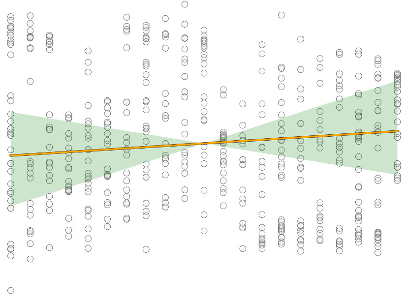
(a)

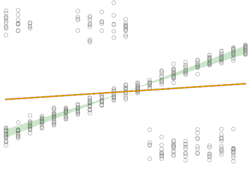
(b)

Figure 1: Datasets with equal contamination rates but different levels of noise $\sigma$. The corruptions are located in the upper left and bottom right parts of both figures. The goal in robust regression is to achieve low square loss on the uncorrupted points. We depict in orange the ordinary least squares estimator and in green the range of linear predictors that would perform comparably to what our algorithms can achieve.

In contrast we will be interested in the setting where $\sigma^{2}$ is much smaller than $R^{2}$, depicted in the right panel of Figure 1. It turns out that existing approaches break down in the sense that they pay an extra factor of $R$ or $R^{2}$ in the clean prediction error (resp. clean regret). Moreover getting around this dependence is a serious obstacle for the usual techniques: we show that regression using any convex surrogate (including Huber loss and $L_{1}$ loss) must pay this price (see Theorem 9.1). Thus our main question is:

Is it algorithmically possible, in the presence of adversarial corruptions, to achieve average clean prediction error (resp. average clean regret) that is independent of $R$?

We answer this question in the affirmative for both online regression with squared loss and linear contextual bandits. Our algorithms succeed where convex surrogates fail, and are based on a novel alternating minimization scheme that interleaves OLS with carefully designed reweighting schemes found through SDPs.

Finally we emphasize that the issue of $R^{2}$ vs. $\sigma^{2}$ dependence is quite relevant in modern reinforcement learning. In particular, there are many sequential tasks where at each step the variance in the losses/rewards is much smaller than the dynamic range. This can happen naturally when there are some catastrophic states that we must avoid, but at no point is the outcome of playing an action in a given state all that uncertain – e.g. when manipulating a robotic arm, some actions can require the application of orders of magnitude more torque. Thus our work may be viewed as a stepping stone towards achieving stronger and more meaningful robustness guarantees in reinforcement learning more broadly.

1.2 Our Results

In this section, we present our main results for both linear regression and contextual bandits in the Huber contamination model. We go on to discuss related work (e.g. robust linear regression under distributional assumptions) in Section 3 below.

Distribution-free offline linear regression with Huber contamination.

We begin by discussing our results in the simplest setting we consider, which is the classical offline linear regression model with a Huber contamination adversary. In the clean version of this model, an arbitrary set of covariates $x_{1},\ldots,x_{n}$ is fixed and clean responses are generated by

$$y_{t}=\langle w^{*},x_{t}\rangle+\xi_{t}$$ (1)

for some mean zero noise $\xi_{t}$; for example, if $\xi_{t}\sim N(0,\sigma^{2})$ then $y_{t}\sim N(\langle w^{*},x_{t}\rangle,\sigma^{2})$. In the Huber contamination model, we relax the assumptions to a total variation distance ball around the generative model. In particular, using the coupling interpretation of total variation distance, this translates into the assumption that with probability $1-\eta$ the response $y_{t}$ is generated by (1) above, and with probability $\eta$ the response $y_{t}$ is sampled from an adversarially chosen noise distribution, which we allow to depend on all other randomness in the problem. In this setting, we obtain the following strong result (and for a fairly simple algorithm, see Technical Overview):

Theorem 1.1 (Informal version of Theorem 5.13 and Theorem 6.9).

Suppose that $\eta<0.499$ is an upper bound on the contamination level, and suppose for some $\sigma\geq 0$ that for all $1\leq t\leq n$, $\|x_{t}\|\leq 1$ and the noise $\xi_{t}$ is conditionally mean-zero and $\sigma^{2}$-subgaussian. Suppose also that $\|w^{*}\|\leq R$. Then if $\eta=0$ or $n\gtrsim\log(\min(n,d))/\eta$, there exists a polynomial time algorithm outputting $w$ satisfying the clean squared loss guarantee

$$\sqrt{\frac{1}{n}\sum_{t=1}^{n}\langle w^{*}-w,x_{t}\rangle^{2}} \lesssim\eta\sigma\sqrt{\log(1/\eta)}+\eta^{1/8}R^{1/2}\sigma^{1/2}(\eta\sqrt{\log(1/\eta)})^{1/4}\sqrt[8]{\frac{\log(\min(n,d))}{n}}$$

$$\quad+\eta^{1/4}R\sqrt[4]{\frac{\log(\min(n,d))}{n}}+\min\left\{\sigma\sqrt{d/n},(R\sigma)^{1/2}\sqrt[4]{1/n}\right\}$$

with high probability.

Note that all but the first term are $o(1)$ as $n\to\infty$. On the other hand, when $\eta=0$ only the last term remains and our result simplifies to standard (minimax optimal) guarantees for Ordinary Least Squares and Ridge regression, see e.g. [Kee10, RH17, SSBD14]. Our result obtains the optimal dependence on $\eta$ up to the $\sqrt{\log(1/\eta)}$ factor, because the information-theoretic lower bound is $\Omega(\eta\sigma)$:

Proposition 1.2.

For any $0\leq\eta<1/2$, any algorithm for Huber-contaminated regression with Gaussian noise must incur clean square loss $\frac{1}{n}\sum_{t=1}^{n}\langle w^{*}-w,x_{t}\rangle^{2}$ at least $\Omega(\eta^{2}\sigma^{2})$.

This follows by embedding the 1-dimensional robust mean estimation problem in a straightforward way — see Example 4.2.

We also show the other aspects of the bound (lower bound on $n$, and the presence of additional “middle terms”) are required — see Example 5.9. Our results generalize naturally to the setting with heavy-tailed noise, even without second moments, and achieve the optimal dependence on $\eta$ in those settings too. We defer the detailed statement of these variants to Section 5.

Impossibility of strengthening the adversary.

Before proceeding to the more sophisticated online settings we consider, we emphasize the impossibility of strengthening the adversary even in the basic model above. First, we consider the version of this problem where the adversary is allowed to corrupt an arbitrary $\eta$ fraction of responses, as opposed to corrupting responses in random locations. In this case, the problem is trivially impossible even in $1$-dimension. If $1-\eta$ fraction of $x_{i}$ are zero and $\eta$ fraction are $1$, $w^{*}=\pm R$, and the adversary corrupts an arbitrary $\eta$ fraction of responses, it’s information-theoretically impossible to tell if $w^{*}=R$ or $w^{*}=-R$. Thus, we have the following lower bound:

Proposition 1.3 (Impossibility with adversarial corruption locations).

In the linear regression model where an adversary corrupts an arbitrary $\eta$ fraction of responses $y_{t}$, any algorithm must suffer clean squared loss $\frac{1}{n}\sum_{t=1}^{n}\langle w^{*}-w,x_{t}\rangle^{2}$ at least $\Omega(\eta R^{2})$.

We note variants of this example have already appeared previously in the literature, see e.g. Lemma 6.1 in [KKM18] or Theorem D.1 in [CAT⁺20]. Similarly, we can consider a strengthened adversary which still corrupts in random locations, but is allowed to change the covariate $x_{t}$ as well as the response $y_{t}$. For essentially the same reason (the adversary can change covariates $x_{t}$ from 0 to 1 and label them with negated responses $y_{t}=\mp R$), it again becomes impossible to tell whether $w^{*}=R$ or $w^{*}=-R$ and so we have a strong impossibility result:

Proposition 1.4 (Impossibility with corrupted covariates).

In the linear regression model where an adversary corrupts an random $\eta$ fraction of covariate and response pairs $(x_{t},y_{t})$, any algorithm must suffer clean squared loss $\frac{1}{n}\sum_{t=1}^{n}\langle w^{*}-w,x_{t}\rangle^{2}$ at least $\Omega(\eta R^{2})$.

Finally, we consider the “breakdown point” assumption $\eta<1/2$. (We wrote $\eta<0.499$ above only to simplify the statement.) If $\eta=1/2$, a special case of our model is a balanced mixture of linear regressions where half of the responses are generated according to linear model $\langle w_{1},x_{t}\rangle+\xi_{t}$ and the other half are generated according to a different linear model $\langle w_{2},x_{t}\rangle+\xi_{t}$. By symmetry, it’s impossible to know which of $w_{1},w_{2}$ is the ground truth linear model, so a clean loss guarantee as in Theorem 1.1 is information-theoretically impossible. In fact, in this setting even list recovery, i.e. outputting both $w_{1}$ and $w_{2}$, is computationally hard [YCS14] and this holds even if $\sigma=0$.

Online linear regression with Huber contamination.

Next, we consider an online version of the linear regression model from before. In this case, the algorithm faces two additional complications compared to before:

1. (Online prediction.) The algorithm is forced to output a prediction $\hat{y}_{t}$ given only $x_{t}$ and the information from previous rounds $(x_{1},y_{1}),\ldots,(x_{t-1},y_{t-1})$, instead of being able to predict based on all of the data.

2. (Adaptive covariates.) Instead of having the covariates $x_{1},\ldots,x_{T}$ fixed in advance, i.e. chosen obliviously, the covariate $x_{t}$ is chosen adaptively by the adversary, based on all information from rounds $1$ to $t-1$. In particular, the algorithm’s choices may affect the future inputs it receives.

Nevertheless, we are able to give a version of our algorithm which deals with both of these issues. The statement below is for the finite-dimensional setting, but we also give a version of the result with no dependence on $d$ (Theorem 7.4), appropriate for the setting of kernel regression. As above, it has an optimal dependence on $\eta$ up to the log factor. In all online settings, we use $T$ for the total number of rounds/covariates to distinguish from the offline setting where we use $n$.

Theorem 1.5 (Robust online regression, informal version of Theorem 7.2).

In the setting of Huber-Contaminated Online Regression (see Definition 1) with subgaussian noise, $\|x_{t}\|\leq 1$ for all $t$ and $\|w^{*}\|\leq R$, for any fixed $\eta<0.499$, there exists an algorithm which runs in time $\mathrm{poly}(n,d)$ and outputs online predictions $\hat{y}_{t}$ which satisfy the following clean square loss regret bound with high probability:

$$\mathop{\textup{Reg}_{\mathsf{HSq}}}(T)=\sum_{t=1}^{T}(\langle w^{*},x_{t}\rangle-\hat{y}_{t})^{2}\lesssim\sigma^{2}\eta^{2}\log(1/\eta)T+\mathrm{poly}(R,\sigma,d,\eta)\cdot o(T).$$ (2)

Online contextual bandits with Huber contamination.

Finally, by combining our online linear regression result with a recent reduction from the contextual bandits literature ([FR20], see Appendix A), we obtain a result for contextual bandits with adaptive contexts and Huber-contaminated losses/rewards. We note that other reductions can probably be applied in the special case of stochastic contexts, e.g. [SLX20], but for simplicity we only state a result in the more general setting with adaptive contexts. First, we describe the interaction model for each round $t$:

1. Nature chooses context $z_{t}=(z_{ta})_{a\in\mathcal{A}}$, possibly adversarially based on the transcript from previous rounds. Here $\mathcal{A}$ with $K\triangleq|\mathcal{A}|$ is the space of possible actions.

2. Learner chooses action $a_{t}$ from $\mathcal{A}$.

3. A $\mathop{\textup{Ber}}(\eta)$ coin $\gamma_{t}$ is flipped to decide whether this round is corrupted.

4. If $\gamma_{t}=0$, i.e. the round is not corrupted, the learner sees loss $\ell^{*}_{t}(a_{t})\triangleq\langle z_{ta},w^{*}\rangle+\xi_{t}$ where $\xi_{t}$ is mean-zero noise.

5. If $\gamma_{t}=1$, i.e. the round is corrupted, the learner sees an arbitrary loss $\ell_{t}(a_{t})$ chosen by an adversary based on $z_{t},a_{t}$, and the transcript from the previous rounds.

In this model, the goal is to minimize the clean regret, that is, to compete with the best policy $\pi$ in hindsight as measured by the true uncorrupted losses. We obtain the following guarantee.

Theorem 1.6 (Robust contextual bandits, informal version of Theorems 8.1 and 8.2).

In the setting of Huber-Contaminated Contextual Bandits (see Definition 2) with $\sigma^{2}$-subgussian noise $\xi_{t}$, for any fixed $\eta<0.499$, there is an algorithm which runs in polynomial time and selects actions $a_{t}$ which satisfy the following clean regret bound with high probability:

$$\mathop{\textup{Reg}_{\mathsf{HCB}}}(T)=\sup_{\pi}\mathop{\mathbb{E}}\left[\sum_{t=1}^{T}(\ell^{*}_{t}(a_{t})-\ell^{*}_{t}(\pi(z_{t})))\right]\lesssim\left(\sigma\eta\sqrt{K\log(1/\eta)}\right)T+\mathrm{poly}(R,K,\eta,\sigma)\cdot o(T)$$ (3)

where the supremum ranges over all (non-adaptive) policies $\pi$, see Preliminaries.

An impossibility result: failure of convex $M$-estimators.

It may appear surprising that our algorithms for dealing with Huber contamination, even in the simplest linear regression setting, do not use an established approach like Huber regression or $L_{1}$/LAD (Least Absolute Deviation) regression — classical approaches which have been studied for decades, and in the case of LAD, even as far back as the 1700s [Bos57]. This is because there are fundamental reasons that neither of these approaches can match our strong guarantees in the distribution-free setting. In fact, we prove a lower bound showing the failure of any $M$-estimator based on a convex loss function:

Theorem 1.7 (Lower bound against convex $M$-estimators, informal version of Theorem 9.1).

There is an instance of Huber-contaminated linear regression where the covariates $x_{t}$ are drawn i.i.d. from a distribution, for which no vector $w$ obtained by minimizing a convex loss with respect to the Huber-contaminated distribution over $(x,y)$’s can achieve square loss better than $\Omega(\eta^{3}R\sigma)$ on the true distribution.

1.3 Roadmap

In Section 2, we give an overview of the main techniques in our approach. In Section 3, we discuss related work in more detail. In Section 4 we record some useful technical facts we use from the literature and state slightly more general versions of the models which we consider. In Section 5, we give an alternating minimization algorithm for solving the offline case of Huber-contaminated linear regression. In Section 6, we give a sum-of-squares algorithm to handle the case of high contamination rate; combined with the result of the previous section, we obtain Theorem 1.1. In Section 7, we give a generic recipe for converting our fixed-design guarantees into online ones, thereby proving Theorem 1.5. In Section 8 we apply the reduction of [FR20] to our regression results to obtain our main result for contextual bandits, Theorem 1.6. Lastly, in Section 9, we prove our lower bound, Theorem 1.7. In Appendix A we verify that the reduction in [FR20] applies to our Huber-contaminated setting.

2 Technical Overview

By a slight modification of the proof of Theorem 5 in [FR20], we can reduce the problem of achieving low clean regret in the contextual bandits setting of Definition 2 to that of producing an oracle for Hubert-contaminated online regression which gets low clean square loss regret. In this section, we overview the main ingredients for producing such an oracle.

There are two main steps: 1) designing an algorithm for fixed-design Huber-contaminated regression that achieves low square loss, and 2) a generic online-to-offline reduction based on cutting plane methods/online gradient descent.

2.1 Huber-Contaminated Fixed-Design Regression

We start with the offline/fixed-design setting, where we are given an arbitrary fixed set of covariates $x_{1},\ldots,x_{n}\in\mathbb{R}^{d}$ and for the indices $t$ for which $y_{t}$ was not corrupted, $y_{t}=\langle w^{*},x_{t}\rangle+\xi_{t}$ for some independent noise $\xi_{t}\sim\mathcal{D}$. The exact assumption on the noise is not so important for the argument, since our algorithm is robust to Huber contamination: given an analysis for bounded noise, all the other versions of the results follow more or less by a straightforward truncation argument, treating heavy-tail events as outliers.

Spectrally Regularized Alternating Minimization.

Similar to existing approaches in the robust statistics literature, our starting point is to formulate an optimization problem that searches for a regressor $w$ and a “structured” subset $S\subset[n]$ of size $(1-O(\eta))n$ over which the clean square loss of $w$ is minimized, i.e.

$$w,S=\mathop{\text{argmin}}_{\begin{subarray}{c}w,S:\\ S\ \text{large and ``structured''}\end{subarray}}\frac{1}{n}\sum_{t\in S}(y_{t}-\langle w,x_{t}\rangle)^{2}.$$ (4)

The subset $S$ should satisfy certain structural properties that the set of uncorrupted points $S^{*}\subseteq[n]$ would collectively satisfy and that can be used to certify that the regressor we use is close to $w^{*}$. Before we describe how the structural property that we use fundamentally differs from the ones exploited in prior works on robust regression, we first discuss our approach to optimizing the nonconvex objective (4). What we do is use a version of a standard heuristic, alternating minimization:

• Given a candidate regressor $w$, we consider the optimization problem

  $$\min_{S}\frac{1}{n}\sum_{t\in S}(y_{t}-\langle w,x_{t}\rangle)^{2}.$$ (5)

  We relax the set of $(1-O(\eta))n$-sized “structured” subsets $S$ to the set of $[0,1]$-valued “structured” weights $\{a_{t}\}_{t\in[n]}$ over the dataset satisfying $\sum_{t}a_{t}=1-O(\eta)$, and it will be apparent from our definition of “structured” below that this can be formulated as a basic SDP.

• Given a candidate set of weights $\{a_{t}\}_{t\in[n]}$, we solve the convex optimization problem

  $$\min_{w}\frac{1}{n}\sum_{t\in S}a_{t}(y_{t}-\langle w,x_{t}\rangle)^{2}.$$ (6)

By repeatedly alternating between these two steps, we arrive at an approximate first-order stationary point $(w,\{a_{t}\})$: more precisely, one for which $\{a_{t}\}$ is optimal given $w$ and for which

$$\frac{1}{n}\sum_{t\in[n]}a_{t}(y_{t}-\langle w,x_{t}\rangle)\langle x_{t},v-w\rangle\leq o(1)$$ (7)

for all $v$ of bounded norm (Lemma 5.7). Of course, this stationary point does not have to be a global optimum of the objective function. Nevertheless, our analysis shows that any stationary point of our objective has strong statistical guarantees (Section 5.4). To show this, we can decompose the left-hand side of (7) for the choice $v=w^{*}$ into two quantities: 1) the contribution from the uncorrupted points, indexed by some subset $T\subset[n]$, and 2) the contribution from the corrupted ones, indexed by $[n]\backslash T$.

In 1), we can pull out the contribution from the quantity $\frac{1}{n}\sum_{t\in T}\langle x_{t},w^{*}-w\rangle^{2}$, which corresponds to the clean square loss achieved by the regressor $w$ we have found and turns out to be the dominant term. To upper bound the rest of 1) and 2), the key technical challenge is respectively to control the error incurred from failing to place nonzero weight $a_{t}$ on some of the points $t\in T$, and from placing nonzero weight $a_{t}$ on some of the points $t\not\in T$. To bound both sources of error, we end up needing to control the quantity

$$\frac{1}{n}\sum_{t\in T}(1-a_{t})\langle x_{t},w^{*}-w\rangle^{2}.$$ (8)

The way in which we do so marks the key distinction between our approach and that of previous works on robust regression.

In prior works (see Section 3 below), this is the place where one could insist that the weights $\{a_{t}\}$ are structured in the sense that along every univariate projection, the empirical moments of the dataset reweighted by $\{a_{t}\}$ are $k$-hypercontractive for some $k\geq 4$, in which case we could use Holder’s to upper bound (8). This is not applicable in the general case, where $x_{1},\ldots,x_{n}$ are arbitrary bounded vectors, so a reweighting with hypercontractive empirical moments may not even exist. Instead, our approach is to insist that $\{a_{t}\}$ must sub-sample the empirical covariance, i.e. that

$$\frac{1}{n}\sum_{t\in[n]}a_{t}x_{t}x_{t}^{\top}\succeq(1-\eta)\frac{1}{n}\sum_{t\in[n]}x_{t}x_{t}^{\top}-o(1)\cdot\textup{Id}$$ (9)

The intuition for this constraint is that because the points that get corrupted in the Huber contamination setting form a random subset of the data, the ideal reweighting $\{a^{*}_{t}\}$ given by placing uniform mass on the true set of uncorrupted points would satisfy this constraint with high probability by standard matrix concentration. So for any $\{a_{t}\}$ which sub-samples the empirical covariance, ignoring the low-order term in (9), we can thus upper bound the quantity (8) by $\eta\sum_{t\in[n]}\langle w^{*}-w,x_{t}\rangle^{2}$. This is negligible compared to the aforementioned dominant term, allowing us to complete the proof that (7) suffices to ensure that $w$ incurs low clean square loss.

Optimal breakdown point via Sum of Squares.

It turns out that the above approach fails for $\eta$ larger than 1/3. Consider a scenario where $1/3$ of the data has been corrupted to come from a different linear model; in this case, there is a spurious local minima in which one takes $w$ in (4) to be the linear model generating the corrupted data and $S$ to consist of the corrupted data and a random half of the uncorrupted data (see Remark 5.3 for further details).

To circumvent this issue, we appeal to a different algorithm when $1/3\leq\eta<1/2$. Our starting point is the observation that another way of circumventing the nonconvexity of (4) is by considering the natural degree-4 sum-of-squares (SoS) relaxation of (4). It turns out that an analysis similar to the one for our alternating minimization algorithm suffices to show that the pseudoexpectation one gets out of solving this relaxation achieves low clean square loss. At a high level, the reason is that one can extract from the former analysis a simple proof in the degree-4 SoS proof system that for $w$ and $S$ satisfying the constraints imposed by the SoS program and optimizing the objective of (4), $w$ achieves low clean square loss. The key difference that allows us to circumvent the bad loss landscape of (4) when $\eta$ is large is that the SoS relaxation is guaranteed to produce a lower bound on the original (unrelaxed) problem (4), whereas the objective value achieved by an arbitrary stationary point need not.

Other extensions.

Using existing generalization bounds [SST10], we give natural and fairly sharp versions of our results for the stochastic/random-design setting. The analysis we outlined works with heavy-tailed noise in $L_{q}$ for any $q>1$ and achieves the optimal dependence on $\eta$ in this setting. If we only use the estimator described above, the sample complexity of our estimator with small confidence parameter $\delta$ is not as good with heavy-tailed noise as with subgaussian noise; we show how to improve the sample complexity when $q\geq 2$ by combining our estimator with a simple median-of-means approach from the heavy-tailed regression literature [HS16, M⁺15].

2.2 Online-to-Offline Reduction

We now explain how to use the guarantee of the previous section to get an algorithm for online regression. At a high level, the idea is to use the fixed-design guarantee above to design a separation oracle between whatever bad predictor we might be using at a particular time step, and the small ball $\mathcal{B}$ of good predictors $w$ around $w^{*}$, any of which would incur sufficiently low regret over any possible sequence of samples. This reduction has a similar spirit to the “halving” algorithm from online learning [SS⁺11], and efficient variants for halfspace learning based on the ellipsoid algorithm [YJY09, TK08].

Concretely, suppose inductively we have seen samples $(x_{1},y_{1}),\ldots,(x_{n},y_{n})$ thus far and have used some vector $w$ to predict in the last $m$ steps where we were given $(x_{n-m+1},y_{n-m+1}),\ldots,(x_{n},y_{n})$. Let $\mathbf{\Sigma}$ be the average of $x_{i}x_{i}^{T}$ over the last $m$ steps. One of two things could be true.

It could be that in these last $m$ steps, $w$ actually performed well, that is, $\lVert w-w^{*}\rVert^{2}_{\mathbf{\Sigma}}$ is small, either because $w\in\mathcal{B}$ or because $x_{n-m+1},\dots,x_{n}$ mostly lie in the slab of space where $w$ and $w^{*}$ yield similar predictions. Either way, because the prediction error under $w$ has been small so far, there is no need to update to a new predictor just yet.

Alternatively, if $\lVert w-w^{*}\rVert^{2}_{\mathbf{\Sigma}}$ is large, then the gradient of the function $w\mapsto\lVert w-w^{*}\rVert^{2}_{\mathbf{\Sigma}}$ would give a separating hyperplane between $w$ and $\mathcal{B}$. Of course, the issue with this is that we don’t know $w^{*}$. To get around this, recall from the fixed-design guarantee that if we ran the alternating minimization algorithm above on the data $(x_{n-m+1},y_{n-m+1}),\dots,(x_{n},y_{n})$ (assuming $m$ is large enough that things concentrate sufficiently well), then the resulting vector $\widetilde{w}$ is close to $w^{*}$ under $\lVert\cdot\rVert_{\mathbf{\Sigma}}$. So to check whether $\lVert w-w^{*}\rVert^{2}_{\mathbf{\Sigma}}$ is large, by triangle inequality we can simply check whether $\lVert w-\widetilde{w}\rVert^{2}_{\mathbf{\Sigma}}$ is large! If so, the gradient of $w\mapsto\lVert w-\widetilde{w}\rVert^{2}_{\mathbf{\Sigma}}$ gives us a separating hyperplane that we can actually compute.

To summarize, the contrapositive of this tells us that if we don’t form a separating hyperplane in a given step, then we know $\lVert w-w^{*}\rVert^{2}_{\mathbf{\Sigma}}$ is small and we are content to continue using $w$. Conversely, if we do form a separating hyperplane, we know we won’t cut $\mathcal{B}$. This is because every point in $\mathcal{B}$ is, by design, close to $w^{*}$ under any norm $\lVert\cdot\rVert_{\mathbf{\Sigma}}$ defined by the empirical covariance $\mathbf{\Sigma}$ of a sequence of samples.

With these two facts in hand, we can safely run a cutting plane algorithm like ellipsoid or Vaidya’s method to update our predictor every time we find a separating hyperplane and ensure that after a bounded number of updates, we find a predictor that will achieve low regret on subsequent steps.

Handling the high-dimensional case.

The above approach does not work when the dimension is unbounded, e.g. in kernelized settings, because the guarantees of cutting plane methods are inherently dimension-dependent. We now describe an alternative approach based on wrapping online gradient descent around our guarantee for Huber-contaminated fixed-design regression.

Instead of using Vaidya’s algorithm to update the vector $w$ that we predict with whenever the separation oracle returns $\nabla\varphi_{t}(w)$, we can imagine updating $w$ by simply stepping in the direction of $-\nabla\varphi_{t}(w)$. The key challenge is to bound the number of times $V$ we get a hyperplane from the separation oracle and have to make such a step, because as long as we don’t receive any new hyperplanes, the predictions we make will incur low square loss. For this, we can appeal to the the fundamental regret bound for online gradient descent [Zin03]. Specifically, if we receive a sequence of convex losses $\varphi_{1},\ldots,\varphi_{V}$ and play a sequence of inputs $w_{1},...,w_{V}$ where $w_{t+1}$ is given by taking a gradient step with respect to $\varphi_{t}$ from $w_{t}$, then the cumulative loss $\sum\varphi_{t}(w_{t})$ incurred only exceeds $\sum\varphi_{t}(w^{*})$ for any single move $w^{*}$ by an $O(\sqrt{V})$ term (see Theorem 7.3). But because the separation oracle is called only when $\varphi_{t}(w_{t})\approx\varphi_{t}-\varphi_{t}(w^{*})$ is large, this immediately implies that $V$ is bounded.

2.3 Lower Bound for Convex Losses

At a high level, the intuition for why convex losses fails is this: in order for the algorithm to be robust to outliers, the loss needs to look roughly like the $L_{1}$ loss (e.g. the Huber loss looks like the $L_{1}$ loss except in a ball near the origin). However, the $L_{1}$ loss $\mathop{\mathbb{E}}[|Y-\langle w,X\rangle|]$ is much less sensitive to making errors for $X$ lying in rare areas of the space than the usual $L_{2}$/squared loss $\mathop{\mathbb{E}}[(Y-\langle w,X\rangle)^{2}]$. In order to take advantage of this, we construct a 1-dimensional example with $1-\Theta(\eta/R)$ fraction of the covariate distribution a delta mass at $1/R$ and the remainder a delta mass at $-1$. For simplicity, we take the noise variance $\sigma=1$. By having the adversary corrupt the response for the much more common portion of the data at $1/R$, the $L_{1}$ regression is tricked into making an order $\eta R$ error on the rare portion of the data, which causes a squared loss of $\Omega((\eta/R)\eta^{2}R^{2})=\Omega(\eta^{3}R)$. By appropriately generalizing this argument, we rule out the success of all convex losses.

3 Related Work

Robust regression, when both the covariates and responses are corrupted

As discussed in Section 1, our work is closely tied to the long line of recent work on designing efficient algorithms for robust statistics in high dimensions. We refer to [Li18, Ste18, DK19] for comprehensive surveys of this literature and focus here on the results related to regression [KKM18, BP20, ZJS20, PJL20, DKK⁺19b, PSB⁺20, DKS19, CAT⁺20]. These works are for the stochastic setting where the covariates are drawn i.i.d. from some distribution $\mathcal{D}_{x}$ but work in a corruption model where the adversary can arbitrarily alter any $\eta$ fraction of the responses and the corresponding covariates. All of these results operate under the assumption that the underlying distribution $\mathcal{D}_{x}$ is either Gaussian or at least 4-hypercontractive. This is not merely an issue of convenience: in the absence of such assumptions, it is impossible to do anything even in one dimension under this corruption model. We recall the following example from the Results section above:

Example 3.1.

Let $d=1$ and $\epsilon=0$, and suppose $w^{*}=R$. Suppose the distribution over covariates is $Ber(\eta)$, i.e. it has $1-\eta$ mass at 0 and $\eta$ mass at 1. Suppose the adversary corrupts an $\eta$ fraction of the pairs $(0,0)$ to be $(1,-R)$. Then it is impossible for the learner to distinguish whether $w^{*}=R$ or $w^{*}=-R$.

We note that variants of this example have already appeared previously in the literature, see e.g. Lemma 6.1 in [KKM18] or Theorem D.1 in [CAT⁺20]. This does not contradict prior results which make distributional assumptions, because they consider the case where $\eta$ is small: when $\eta=o(1)$, $Ber(\eta)$ is no longer $O(1)$-hypercontractive as its fourth moment is $\eta R^{4}$ while the square of its second moment is $\eta^{2}R^{4}$. In summary: when there exist rare features in the data, or when the corruption fraction $\eta$ is large, it is simply not information-theoretically possible to handle corruption in the covariates.

We also note that the work of [PJL20] shows that, at least in some cases, the covariate corruption can be handled separately from the response corruption by first running a standard filtering method on the covariates, and second running a method robust to response outliers (in their case, Huber regression) on the remaining data. This suggests that handling covariate corruption (when it is possible) and response corruption may be largely orthogonal problems. Finally, one commonality with our work and much of the previous literature is the use of Sum of Squares programming (for us, only needed near the breakdown point $1/2$); however, we use a fairly simple degree-4 SoS program, as opposed to prior work (e.g. [KKM18, BP20]) where the SoS degree and sample complexity need to be large in order to take advantage of stronger regularity assumptions.

Robust regression, when just the responses are corrupted

A milder corruption model which has received significant attention in the statistics literature is the setting where a fraction, either randomly or adversarily chosen, of the responses are corrupted, while the covariates are left intact. One popular approach for regression in this setting is M-estimation [L⁺17, ZBFL18], originally introduced by Huber [Hub64], in which one minimizes a loss function with suitable robustness properties. Common choices of loss function include the $L_{1}$ loss and the Huber loss. In addition to the earlier asymptotic results for this approach [BJK78, Hub73, Pol91], by now numerous works have obtained non-asymptotic guarantees for M-estimation under a variety of models for how the responses are corrupted, but predominantly under the assumption that the design is sub-Gaussian or similarly structured [KP18, DT19, SF20, dNS20]. Notably, in [DT19, SF20] it was shown that in the setting of sparse linear regression with Huber-contaminated responses, M-estimation with ($\ell_{1}$-regularized) Huber loss is nearly minimax-optimal when the noise distribution $\mathcal{D}$ and the covariates are i.i.d. Gaussian.

One exception, and perhaps the result closest in spirit to our results for regression, is that of [Chi20]. One consequence of the results in this work is that in the random-design setting of Definition 1, that is when the covariates are drawn i.i.d. from some distribution $\mathcal{D}_{x}$, then if the function class (equivalently, covariate distribution) is hypercontractive in the sense that for any $w\in\mathcal{W}$, $\mathop{\mathbb{E}}_{\mathcal{D}_{x}}[\langle w-w^{*},x\rangle^{p}]^{2/p}\leq\mathop{\mathbb{E}}_{\mathcal{D}_{x}}[\langle w-w^{*},x\rangle^{2}]$ for some $p>2$, and if the noise distribution $\mathcal{D}$ satisfies suitable conditions, then M-estimation with Huber loss achieves the information-theoretically optimal error of $\Theta(\sigma^{2}\eta^{2})$ in squared loss. It is also possible to modify their proof to show that the same algorithm would yield the information-theoretically optimal error of $\Theta(\sigma\eta)$ in a different metric, the $L_{1}$ loss, without the hypercontractivity condition. An $L_{1}$ guarantee is much weaker than the usual $L_{2}$ (i.e. squared loss) guarantee: for example, it is too weak to give anything interesting for the contextual bandits application.

In fact, as we show in Theorem 9.1, M-estimation with Huber loss, and more generally minimization of any convex surrogate loss, will not achieve squared loss $\Theta(\sigma^{2}\eta^{2})$ in general when the function class/covariate distribution fails to satisfy this hypercontractivity condition. Instead, we show such estimators must pay squared loss at least $\Omega(\sigma R\eta^{3})$. We also mention that to our knowledge, the only work that has explicitly considered online regression with corruptions is [PF20], where they considered Gaussian covariates and a random fraction of responses are corrupted by an oblivious shift. Additionally, another notable line of work to mention in the literature on regression with contaminated responses stems from using hard thresholding [BJK15, BJKK17, SBRJ19], though these works work also make strong regularity assumptions on the covariates.

Lastly, we mention that in the context of classification, there have been a number of recent works giving new algorithmic results for corruption models where the binary labels are corrupted by some process that is halfway between purely stochastic and purely adversarial. For instance, [DGT19, CKMY20, DKTZ20] focus on the Massart noise model which can essentially be viewed as a setting where an adversary can only control a random fraction of the labels, but can change them in an arbitrary way. This can be thought of as the classification version of the Huber-contaminated regression problem that we consider in the present work, and the former two results work in the setting without distributional assumptions. We also note that the recent work of [DKK⁺20] considers the stronger model of Tsybakov noise and obtains polynomial-time algorithms under distributional assumptions.

Robustness for bandits

There have been a number of notions of robustness proposed in the bandits literature. A classic notion is that of adversarial bandits, a setting where one would like to prove regret bounds even when the rewards are chosen adversarially [ACBFS02]. Many papers have worked to identify ways of interpolating between fully adversarial rewards and stochastically generated ones, including the line of work on “best of both worlds” results [BS12, SS14, AC16, SL17] as well as an interesting model of bandits with adversarial corruptions introduced by [LMPL18] and subsequently studied by [GKT19]. The latter is a setting of multi-armed bandits where rewards are generated stochastically but then perturbed by an adaptive adversary with a fixed budget of how much he can move the rewards in any given sample path. We stress that the setting of adversarial bandits is orthogonal to the thrust of the present work, where the goal is to get small clean regret. For example, while the adversarial nature of the rewards makes the former quite challenging, it is still possible to achieve sublinear regret for adversarial bandits, whereas in our setting, one cannot do better than $\Omega(\eta^{2}\sigma^{2}T)$.

Other notions of robustness that have been considered include the standard notion of misspecification (e.g. [FR20, NO20]) as in Definition 2, as well as the notion of heavy-tailed reward distributions [BCBL13]. The setting of Huber-contaminated rewards that we study was previously studied in the multi-armed case by [KPK19, ABM19]. [KPK19] also studied Huber-contaminated linear contextual bandits when the contexts are Gaussian or collectively satisfy some RSC-like condition. Even in this distribution-specific setting, their analysis loses a factor of $R$. A recent work [AGKS21] also studied the Gaussian context case of Huber-contaminated linear contextual bandits and improved over [KPK19]; however their result also suffers from a dependence on $R$. Lastly, we mention the work of [SS14, ZS19] who considered a different corruption model for the multi-armed case where the contaminations cannot reduce the “gap,” i.e. the difference between the reward of the best arm and that of any other arm, by more than a constant factor in any time step.

4 Preliminaries

4.1 Formal Description of Models

For technical reasons which will appear naturally in the analysis, it is useful for us to consider the general misspecified model where $\epsilon\geq 0$ is a misspecification parameter that accommodates deviation between the true prediction rule and the best linear model. However, the reader should feel free to consider the usual well-specified setting $\epsilon=0$ when reading the results.

Robust Offline Regression.

Our analysis in the oblivious setting allows the corruption adversary to depend arbitrarily on the randomness in the problem, as in e.g. [Chi20]. This is different from in the online setting, where it’s important that all of the randomness respects the filtration corresponding to time. To be clear, we define the offline model explicitly here.

1. Covariates $x_{1},\ldots,x_{n}$ are arbitrary fixed vectors in the unit ball of $\mathbb{R}^{d}$, i.e. they are chosen obliviously.

2. For every $t$ from $1$ to $n$, a $Ber(\eta)$ coin is flipped to determine if round $t$ is corrupted or not. Let $a^{*}_{t}$ be the indicator for whether round $t$ was uncorrupted, i.e. $a^{*}_{t}=1$ when the round is not corrupted and this occurs with probability $1-\eta$.

3. For every uncorrupted round, we observe $y_{t}$ given by

   $$y_{t}=y^{*}_{t}+\xi_{t},\qquad y^{*}_{t}=\langle w^{*},x_{t}\rangle+\epsilon_{t}$$ (10)

   where $w^{*}$ is the true regressor and $\|w^{*}\|\leq R$, and $\xi_{t}$ is independently sampled from the noise distribution $\mathcal{D}$ and $\lvert\epsilon_{t}\rvert\leq\epsilon$ is the misspecification. The misspecification $\epsilon_{t}$ can be chosen in a completely adversarial fashion: formally, it is a random variable depending arbitrarily on all other randomness in the setup (e.g. it can depend arbitrarily on the noise and the coin flips from all rounds).

4. For every corrupted round, $y_{t}$ is chosen freely by the adversary. Again, we assume nothing about $y_{t}$ – it can depend arbitrarily on all other randomness in the problem.

Robust Online Regression.

We begin by introducing the setup for the online linear regression problem, which is closely related to the linear contextual bandits problem we introduce later. Online regression itself is one of the fundamental problems in online learning that has been extensively studied in the uncontaminated setting, see e.g. [Vov01, AW01, CBL06].

Definition 1 (Huber-Contaminated Online Regression).

Fix Huber contamination rate $\eta\in(0,1/2)$, misspecification bound $\epsilon$, noise distribution $\mathcal{D}$, and unknown weight vector $w^{*}$. In each round $t\in[T]$:

1. Nature chooses input $x_{t}\in\mathbb{R}^{d}$, possibly adversarially based on the transcript from previous rounds.

2. Learner chooses prediction $\widehat{y}_{t}$.

3. A $\mathop{\textup{Ber}}(\eta)$ coin is flipped to decide whether this round is corrupted.

4. If the round is not corrupted, sample $\xi_{t}$ independently from $\mathcal{D}$. The learner sees $y_{t}\triangleq y^{*}_{t}+\xi_{t}$, where $y^{*}_{t}\triangleq\langle w^{*},x_{t}\rangle+\epsilon_{t}$ for some quantity $\epsilon_{t}(x_{t})$ satisfying $\lvert\epsilon_{t}(x_{t})\rvert\leq\epsilon$.

5. If the round is corrupted, the learner sees an arbitrary $y_{t}$ chosen by an adversary based on $x_{t}$ and the transcript from the previous rounds.

The goal of the learner, given any $x_{t}$ in round $t$ (and the transcript from the previous rounds), is to choose a prediction $\widehat{y}_{t}$ such that with high probability over the choice of $\mathop{\textup{Ber}}(\eta)$ coins, and for any (possibly adaptively chosen) sequence of feature vectors $\{x_{1},\ldots,x_{T}\}$ in the above model, the quantity

$$\mathop{\textup{Reg}_{\mathsf{HSq}}}(T)=\sum^{T}_{t=1}(\widehat{y}_{t}-y^{*}_{t})^{2}.$$ (11)

is small. We say that $A$ achieves clean square loss regret $\mathop{\textup{Reg}_{\mathsf{HSq}}}(T)$. Note that $\mathop{\textup{Reg}_{\mathsf{HSq}}}$ is a random variable depending on the randomness of the $\mathop{\textup{Ber}}(\eta)$ coins, the randomness of the noise $\xi_{t}$, any stochasticity in the choice of the inputs $x_{t}$, and the randomness of the learner and adversary. We will establish high-probability bounds on this random variable.

Remark 4.1 (Clean vs Dirty Loss).

It is very important to note that the goal for robust statistics is to minimize the clean square loss $\sum_{t=1}^{T}(\hat{y}_{t}-y^{*}_{t})^{2}$ and not the “dirty” square loss $\sum_{t=1}^{T}(\hat{y}_{t}-y_{t})^{2}$ where $y_{t}$ is potentially corrupted. If our goal was to try to fit the corruptions, as in agnostic learning, then using Ordinary Least Squares would be a good approach for this regression problem.

On the other hand, there is no importance difference between optimizing the noisy clean square loss $\sum_{t=1}^{T}(\hat{y}_{t}-(y^{*}_{t}+\xi_{t}))^{2}$ and the clean square loss as defined above. Because the noise is by definition independent of $\hat{y}_{t},y^{*}_{t}$, we know that in expectation $\mathop{\mathbb{E}}[\sum_{t=1}^{T}(\hat{y}_{t}-(y^{*}_{t}+\xi_{t}))^{2}]=\mathop{\mathbb{E}}[\sum_{t=1}^{T}(\hat{y}_{t}-y^{*}_{t})^{2}]+\sigma^{2}T$ and so the additive term coming from the noise doesn’t depend on the prediction sequence $\hat{y}_{t}$.

Connection to robust mean estimation

Note that regression with Huber contaminations is at least as hard as the problem of mean estimation under Huber contaminations, implying that achieving sublinear regret for Huber-contaminated online regression is impossible:

Example 4.2.

Let $d=1$ and $\epsilon=0$, and suppose $w^{*}=R$ and $\mathcal{D}=\mathcal{N}(0,\sigma^{2})$. Suppose we only ever see $x_{t}=1$, so that we always have $y^{*}_{t}=R$. Then each uncorrupted $y_{t}$ is simply an independent draw from $\mathcal{N}(R,\sigma^{2})$, so the question of producing a good predictor $\widehat{y}$ in this special case is equivalent to that of estimating the mean of a univariate Gaussian with variance $\sigma^{2}$ under the Huber contamination model. It is known that one cannot do this to error better than $\Omega(\eta\sigma)$ (see [DKK⁺18]). More generally, if we only assume $\mathcal{D}$ has hypercontractive moments up to degree $k$, one can devise distributions $\mathcal{D}$ for which one cannot do better than error $\Omega(\eta^{1-1/k}\sigma)$ (see e.g. Fact 2 from [HL19]).

Robust Contextual Bandits.

We study the following robust version of contextual bandits, first introduced in [KPK19]. We first state the general form of the contextual bandits model (for an abstract regression function $f$), then specialize to the linear case.

Definition 2 (Huber-Contaminated Contextual Bandits).

Let $\mathcal{Z}$ be an arbitrary state space, and let $\mathcal{A}$ be an action space of size $K$. Fix Huber contamination rate $\eta\in(0,1/2)$, misspecification rate $\epsilon$, and unknown function $f:\mathcal{Z}\times\mathcal{A}\to{\mathbb{R}}$. Ahead of time, an oblivious adversary chooses distributions $\mathop{\mathbb{P}}_{\ell^{*}_{t}}[\cdot|z_{t}]$ over loss functions $\ell^{*}_{t}:\mathcal{A}\to[0,R]$ for all possible contexts $z_{t}$ and all time steps $t\in[T]$. We assume the conditional means of the loss distributions are realized up to misspecification $\epsilon$ by $f$, i.e. for all $t,z,a$,

$$\mathop{\mathbb{E}}_{\ell^{*}_{t}}[\ell^{*}_{t}(a)|z_{t}=z]=f(z,a)+\epsilon_{t}(z,a),\qquad\lvert\epsilon_{t}(z,a)\rvert\leq\epsilon.$$ (12)

Let $\xi_{t}$ be the random variable which, conditioned on $z_{t}=z$, takes on the value

$$\xi_{t}\triangleq\ell^{*}_{t}(a)-f(z,a)-\epsilon_{t}(z,a),$$ (13)

and define noise parameter $\sigma$ by $\sigma^{2}\triangleq\sup_{z,t}\mathop{\mathbb{E}}[\xi_{t}^{2}|z_{t}=z]$. In each round $t\in[T]$:

1. Nature chooses $z_{t}$, possibly adversarially based on the transcript from previous rounds.

2. Learner chooses action $a_{t}\in\mathcal{A}$.

3. A $\mathop{\textup{Ber}}(\eta)$ coin $\gamma_{t}$ is flipped to decide whether this round is corrupted.

4. If $\gamma_{t}=0$, i.e. the round is not corrupted, the learner sees loss $\ell^{*}_{t}(a_{t})$, where $\ell^{*}_{t}$ is drawn independently from the distribution $\mathop{\mathbb{P}}_{\ell^{*}_{t}}[\cdot|z_{t}]$.

5. If $\gamma_{t}=1$, i.e. the round is corrupted, the learner sees an arbitrary loss $\ell_{t}(a_{t})$ chosen by an adversary based on $z_{t},a_{t}$, and the transcript from the previous rounds.

The goal of the learner in the adversarial setting is to compete with the best policy in hindsight as measured by the clean losses $\ell^{*}_{t}$ incurred in every round, that is to select a sequence of actions $a_{1},\dots,a_{T}$ for which

$$\widetilde{\mathop{\textup{Reg}_{\mathsf{HCB}}}}(T)=\sup_{\pi}\mathop{\mathbb{E}}\left[\sum^{T}_{t=1}\left(\ell^{*}_{t}(a_{t})-\ell^{*}_{t}(\pi(z_{t}))\right)\right],$$ (14)

is small, where the supremum ranges over all (non-adaptive) policies $\pi:\mathcal{X}\to\mathcal{A}$ and the expectation is over the randomness of the $\mathop{\textup{Ber}}(\eta)$ coins, the randomness of the rewards, any stochasticity in the choice of contexts, and the randomness of the learner. We say that such a learner achieves clean pseudo-regret $\widetilde{\mathop{\textup{Reg}_{\mathsf{HCB}}}}(T)$.

In the special case where $\epsilon=0$, we will consider the quantity

$$\mathop{\textup{Reg}_{\mathsf{HCB}}}(T)=\sum^{T}_{t=1}\left(\ell^{*}_{t}(a_{t})-\ell^{*}_{t}(\pi^{*}(z_{t}))\right)$$ (15)

where $\pi^{*}(z)\triangleq\arg\max_{a}f(z,a)$. Note that this is a random variable in the same things defining the expectation in (14). We say that a learner achieves clean regret $\mathop{\textup{Reg}_{\mathsf{HCB}}}(T)$. We will establish high-probability bounds on $\mathop{\textup{Reg}_{\mathsf{HCB}}}$.

Definition 3 (Huber-Contaminated Linear Contextual Bandits).

This is the special case of Definition 2 where the regression function $f:\mathcal{X}\times\mathcal{A}\to\mathbb{R}$ is linear in the following sense. The context space $\mathcal{X}$ is a Hilbert space and each context is of the form $z_{t}=(z_{t1},\ldots,z_{tK})$, i.e. there is a separate context vector for each arm. Then we assume that

$$f(z,a)=\langle z_{ta},w^{*}\rangle$$

for some vector $w^{*}\in\mathbb{R}^{d}$.

Without adversarial corruptions this is the familiar linear contextual bandits problem, which has a wide range of applications precisely because in many settings the context is an important component of the prediction task. For example, in online advertising the choice of which ad to display ought to depend on information about the webpage that the ad will be displayed on as well as any information we have about the user we are displaying it to, which can be encoded as a high-dimensional vector. In healthcare, when we want to choose between various treatment options again we want to adapt to the relevant context such as the patient history. For additional applications, see the survey [BR19].

However in many of these settings it is natural to imagine that some of the feedback we receive departs in arbitrary ways from the model. This could happen in online advertising due to clickfraud, particularly when malware takes over a user’s account. It could happen in healthcare in the context of drug trials, particularly ones that measure some real valued variable, when there are testing errors or confounding variables that are difficult to model. For all these and many more reasons it is natural to wonder if there could be algorithms for contextual bandits with stronger robustness guarantees.

Remark 4.3.

We note that in some papers on contextual bandits, the range of the loss functions is normalized to $[0,1]$ for convenience. The scale-invariant quantity which we want to avoid dependence on is the ratio $R/\sigma$.

Remark 4.4.

As we will rely on a formal connection between contextual bandits and online regression illuminated in [FR20], it will be helpful to situate our definitions in their context. In particular, when $\eta=0$, Definition 2 specializes to Assumption 4 of [FR20], and an algorithm for Definition 1 achieving clean square loss regret at most $\mathop{\textup{Reg}_{\mathsf{HSq}}}(T)$ would satisfy Assumption 2b of [FR20] in the realizable case with $\epsilon$-misspecification.

Model Assumptions.

We adopt the following standard normalization convention for the covariates and weight vector.

Assumption 1.

In the regression setting (Definition 1), for any round $t$, $\lVert x_{t}\rVert\leq 1$ almost surely, $\lVert w^{*}\rVert\leq R$. Correspondingly, in the contextual bandits setting (Definition 3) we assume $\lVert z_{ta}\rVert\leq 1$ for all $a$ and $\lVert w^{*}\rVert\leq R$.

To simplify the statement of bounds we assume in all statements that $\epsilon,\sigma=O(R)$. The last assumption can be removed at the cost of longer Theorem statements (e.g. writing $R+\sigma$ instead of $R$); this scaling captures the interesting setting for the bounds, because if $\epsilon\gg R$ then the responses are arbitrary, and if $\sigma\gg R$ then no interesting robustness guarantee is possible, as explained earlier — the trivial guarantee of Ordinary Least Squares in this setting is already close to optimal.

We now formally describe the (weak) assumptions on the noise under which we can perform our analysis.

Definition 4 (Weak $L_{q}$ Space).

Suppose $X$ is a real-valued random variable and $q\geq 1$. We define the weak $L_{q}$ or $L_{q,\infty}$ quasinorm of $\xi$ to be

$$\|X\|_{q,\infty}\triangleq\sup_{\lambda>0}\lambda\cdot\left|\mathop{\mathbb{P}}[|X|>\lambda]^{1/q}\right|$$

so that $\mathop{\mathbb{P}}[|X|>\lambda]\leq\|X\|_{q,\infty}^{q}/\lambda^{q}$. When $q=\infty$, we define $\|X\|_{\infty,\infty}=\inf\{\lambda>0:\mathop{\mathbb{P}}[|X|\geq\lambda]=0\}$ to be the same as the $L_{\infty}$ norm. We say that $X$ is in weak $L_{q}$ or $L_{q,\infty}$ space if $\|X\|_{q,\infty}<\infty$.

From Markov’s inequality, one has that $\mathop{\mathbb{P}}[|X|>\lambda]\leq\mathop{\mathbb{E}}[|X|^{q}]/\lambda^{q}$ which shows that $\|X\|_{q,\infty}\leq\|X\|_{q}$.

Assumption 2.

We assume the noise $\xi\sim\mathcal{D}$ is mean zero and that for some $q>1$,

$$\sigma_{q}\triangleq\|\xi\|_{q,\infty}<\infty.$$

4.2 Technical Preliminaries

Here we collect miscellaneous technical facts that will be useful in later sections. Throughout this paper we use standard notation for inequalities up to constants; for example, $a\lesssim b$ and $a=O(b)$ both denote an inequality true up to an absolute constant, and occasionally we use $C>0$ to denote a universal constant which can change from line to line. Given a matrix $M$, we let $\lVert M\rVert$ denote the operator norm of $M$. Given a positive semidefinite matrix $\mathbf{\Sigma}$, we define the Mahalanobis norm by

$$\|x\|_{\mathbf{\Sigma}}^{2}:=\|\mathbf{\Sigma}^{1/2}x\|^{2}=\langle x,\mathbf{\Sigma}x\rangle.$$ (16)

Concentration of measure.

We use some concentration inequalities which we state here. We use standard martingale terminology, see e.g. [Dur19]; in particular, we say that a sequence of random variables $X_{1},\ldots,X_{t}$ adapted to a filtration $\mathcal{F}_{t}$ form a martingale difference sequence if $\mathop{\mathbb{E}}[X_{t}|\mathcal{F}_{t-1}]=0$ for all $t$. We say a mean-zero random variable $X$ is $\sigma^{2}$-subgaussian if $\log\mathop{\mathbb{E}}[e^{\lambda X}]\leq\lambda^{2}\sigma^{2}/2$ for all $\lambda\in\mathbb{R}$; recall that if $|X|\leq K$ then $X$ is $O(K^{2})$-subgaussian [Ver18].

Fact 4.5 (Azuma-Hoeffding inequality).

Suppose that $X_{1},\ldots,X_{n}$ is a martingale difference sequence and $|X_{i}|\leq M_{i}$ almost surely. Then

$$\mathop{\mathbb{P}}\left[\frac{1}{n}\sum^{n}_{i=1}X_{i}\geq t\right]\leq\exp\left(-\Omega\left(\frac{nt^{2}}{\frac{1}{n}\sum_{i}M_{i}^{2}}\right)\right)$$ (17)

Fact 4.6 (Bernstein’s inequality).

For $X_{1},...,X_{n}$ independent and mean-zero, if $\lvert X_{i}\rvert\leq M$ for all $i$, then for all $t>0$,

$$\mathop{\mathbb{P}}\left[\frac{1}{n}\sum^{n}_{i=1}X_{i}\geq t\right]\leq\exp\left(-\Omega\left(\frac{nt^{2}}{\frac{1}{n}\sum\mathop{\mathbb{E}}[X_{i}^{2}]+Mt}\right)\right)$$ (18)

We will use the following general version of the Azuma-Hoeffding inequality, which applies to martingales in Euclidean space of arbitrary dimension with subgaussian step sizes. (Note: this result is false if we consider martingales with steps that are general subgaussian vectors, which can make steps of size $\sqrt{d}$ in dimension $d$.) This result follows from the same proof as Equation 5.18 in [KS91], with some small differences: there they consider bounded variation processes instead of discrete-time martingales. In the bounded step size case, optimal constants were obtained in [Pin94]. For completeness, we prove Theorem 4.7 in the Appendix.

Theorem 4.7 (Subgaussian-step vector Azuma-Hoeffding, cf. Equation 5.18 in [KS91]).

Suppose that $X_{1},\ldots,X_{n}$ are random vectors in Euclidean space with $\|X_{t}\|\leq 1$ almost surely for all $t$, and $\xi_{1},\ldots,\xi_{n}$ are random variables such that almost surely, the law of $\xi_{t}$ conditional on $X_{1},\ldots,X_{t},\xi_{1},\ldots,\xi_{t-1}$ is mean-zero and $\sigma^{2}$-subgaussian. Then

$$\mathop{\mathbb{P}}\left[\left\|\frac{1}{n}\sum^{n}_{i=1}\xi_{i}X_{i}\right\|\geq u\right]\leq 2\exp\left(-\Omega\left(\frac{nu^{2}}{\sigma^{2}}\right)\right).$$ (19)

Matrix concentration.

A key ingredient in our argument is concentration for matrix martingales. See [Tro12, Tro11] for background on matrix concentration; for infinite dimensional settings we use a version of matrix concentration which depends on effective dimension [HKZ⁺12, Min17]. To briefly recall, a matrix martingale $\mathbf{Y}_{1},\ldots,\mathbf{Y}_{n}$ adapted to a filtration $\mathcal{F}_{t}$ with difference sequence $\mathbf{X}_{t}$ is an $\mathcal{F}_{t}$-adapted process satisfying $\mathbf{Y}_{t}=\sum_{s=1}^{t}\mathbf{X}_{s}$ and $\mathop{\mathbb{E}}[\mathbf{X}_{t}|\mathcal{F}_{t-1}]=0$. We also recall that for a function $f:\mathbb{R}\to\mathbb{R}$ and symmetric matrix $M$ with eigendecomposition $M=\sum_{i}\lambda_{i}\rho_{i}\rho_{i}^{T}$, the notation $f(M)$ corresponds to applying $f$ to the spectrum, i.e. $f(M)=\sum_{i}f(\lambda_{i})\rho_{i}\rho_{i}^{T}$.

Theorem 4.8 (Matrix Freedman Inequality, [Min17]).

Suppose $\mathbf{Y}_{1},...,\mathbf{Y}_{n}\in{\mathbb{R}}^{d\times d}$ is a symmetric matrix martingale adapted to filtration $\mathcal{F}_{t}$, whose associated difference sequence $\{\mathbf{X}_{t}\}$ satisfies $\lVert\mathbf{X}_{t}\rVert\leq 1$ almost surely for all $t$. Let $\mathbf{W}=\sum_{t}\mathop{\mathbb{E}}[\mathbf{X}_{t}^{2}|\mathcal{F}_{t-1}]$, then for any $t\geq\frac{1}{6}(1+\sqrt{1+36\sigma_{n}^{2}})$

$$\mathop{\mathbb{P}}[\|\mathbf{Y}_{n}\|\geq t\text{ and }\|\mathbf{W}\|\leq\sigma_{n}^{2}]\leq 50d_{1}(t)\cdot\exp\left(\frac{-t^{2}/2}{\sigma_{n}^{2}+t/3}\right)$$

where

$$d_{1}(t)=\mathop{\textup{Tr}}f(t\mathop{\mathbb{E}}[\mathbf{W}]/\sigma_{n}^{2})$$

and $f(x)=\min(1,x)$.

Corollary 4.9.

In the same setting as Theorem 4.8, suppose that for some $\sigma\leq 1$, $\mathop{\mathbb{E}}[\mathbf{X}_{t}^{2}|\mathcal{F}_{t-1}]\preceq\sigma^{2}$ almost surely. Then for any $u\geq 1/18n+\sigma\sqrt{1/n}$

$$\mathop{\mathbb{P}}[\|(1/n)\cdot\mathbf{Y}_{n}\|\geq u]\leq 50d_{2}(u)\cdot\exp\left(\frac{-nu^{2}/2}{\sigma^{2}+u/3}\right)$$

where

$$d_{2}(u)=\mathop{\textup{Tr}}f(u\mathop{\mathbb{E}}[\mathbf{W}]/\sigma^{2})$$

and $f(x)=\min(1,x)$ as in Theorem 4.8.

Proof.

Apply Theorem 4.8 with $t=nu$ and $\sigma_{n}^{2}=n\sigma^{2}$, noting that $d_{2}(u)=d_{1}(nu)$; in this statement, we only strengthened the assumed lower bound on $t$. ∎

Truncation Lemma.

In our algorithm and analysis, we handle heavy-tailed noise using a truncation argument; this somewhat parallels the use of truncation arguments in large deviation theory, see e.g. [FN71]. The following Lemma shows that random variables with tail bounds behave reasonably under truncation, in the sense that their means do not move drastically.

Lemma 4.10.

Suppose that $X$ is a mean-zero random variable and $\sigma_{q}\triangleq\|X\|_{q,\infty}<\infty$. Then for any $s>0$,

$$|\mathop{\mathbb{E}}[X\mathop{\mathds{1}}[|X|<s]]|\leq\frac{q}{q-1}\cdot\frac{\sigma_{q}^{q}}{s^{k-1}}.$$

Proof.

We know

$$0=\mathop{\mathbb{E}}[X]=\mathop{\mathbb{E}}[X\mathop{\mathds{1}}[|X|<s]]+\mathop{\mathbb{E}}[X\mathop{\mathds{1}}[|X|\geq s]]$$

so using the identity $\mathop{\mathbb{E}}[Z]=\int_{0}^{\infty}\mathop{\mathbb{P}}[Z>y]dy$ for nonnegative random variable $Z$ (Lemma 1.2.1 of [Ver18]), we have

$$|\mathop{\mathbb{E}}[X\mathop{\mathds{1}}[|X|<s]]|=|\mathop{\mathbb{E}}[X\mathop{\mathds{1}}[|X|\geq s]]| \leq\mathop{\mathbb{E}}[|X|\mathop{\mathds{1}}[|X|\geq s)]]$$

$$=\int_{0}^{\infty}\mathop{\mathbb{P}}[|X|\mathop{\mathds{1}}[|X|\geq s]>y]dy$$

$$=s\mathop{\mathbb{P}}[|X|\geq s]+\int_{s}^{\infty}\mathop{\mathbb{P}}[|X|>y]dy$$

$$\leq\frac{\sigma_{q}^{q}}{s^{q-1}}+\int_{s}^{\infty}\frac{\sigma_{q}^{q}}{y^{k}}dy$$

$$=\sigma_{q}^{q}\left(\frac{1}{s^{q-1}}+\frac{1}{(q-1)s^{q-1}}\right)=\frac{q}{q-1}\cdot\frac{\sigma_{q}^{q}}{s^{k-1}}$$

where in the last inequality, we used the definition of $L_{q,\infty}$. ∎

5 Alternating Minimization for Offline Regression

In this section, we prove our main results for regression in the usual offline setting. After giving some setup and stating the main offline result in Section 5.1, in Section 5.2 we give a full description of our alternating minimization-based algorithm. In Section 5.3 we show that it converges to an approximate stationary point. In Section 5.4 we show that this suffices to obtain our claimed error guarantees, and also give improved rates in the case of subgaussian noise. In Section 5.5 we show how our fixed-design guarantee can yield strong results in the stochastic setting often considered in statistical learning. Finally, in Section 5.6, we give improved rates when the noise is in $L_{q}$ for $q\geq 2$ by boosting via a high-dimensional median.

5.1 Setup and Main Result

We will state and prove results for two closely related settings: (1) the usual setting in linear regression where the covariates $x_{t}$ are fixed arbitrary vectors (i.e. chosen obliviously), and (2) the model which is relevant for our online applications, where the covariates $x_{t}$ are generated sequentially and adaptively, so they can depend on e.g. the realization of the noise in previous rounds. The second setting is the proper offline version of the Huber-Contaminated Online Regression Problem as defined in Definition 1.

We briefly recall some of the relevant notation. Let $a^{*}_{t}$ be the indicator for whether round $t$ was uncorrupted, i.e. $a^{*}_{t}=1$ when the round is not corrupted and this occurs with probability $1-\eta$. Recall from (11) that for every $t\in[n]$ corresponding to a round which is not corrupted, we observe $y_{t}$ given by

$$y_{t}=y^{*}_{t}+\xi_{t},\qquad y^{*}_{t}=\langle w^{*},x_{t}\rangle+\epsilon_{t}$$ (20)

where $w^{*}$ is the true regressor and $\|w^{*}\|\leq R$, and $\xi_{t}$ is independently sampled from the noise distribution $\mathcal{D}$, and $\lvert\epsilon_{t}\rvert\leq\epsilon$ is the misspecification. On the other hand, on corrupted rounds $y_{t}$ is chosen freely by the adversary. For convenience, define

$$\mathbf{\Sigma}_{n}\triangleq\frac{1}{n}\sum^{n}_{t=1}x_{t}x_{t}^{\top}$$ (21)

Let $u^{*}$ be the best norm $R$ linear predictor of the uncorrupted and unnoised data, that is,

$$u^{*}\triangleq\arg\min_{u:\|u\|\leq R}\frac{1}{n}\sum_{t}(y^{*}_{t}-\langle u,x_{t}\rangle)^{2}$$ (22)

and let $\delta_{t}\triangleq y^{*}_{t}-\langle u^{*},x_{t}\rangle$. By definition of $u^{*}$, we have that

$$\frac{1}{n}\sum_{t}\delta^{2}_{t}\leq\frac{1}{n}\sum_{t}\epsilon^{2}_{t}\leq\epsilon^{2}$$ (23)

almost surely; in fact, the conclusion of (23) is all we need about the misspecification model and $w^{*},\epsilon_{t}$ play no further role in this section.

Our goal will be to output $\widehat{w}$ such that the MSE (Mean Squared Error) with respect to the true responses is as small as possible; since $u^{*}$ is the optimal linear predictor, this is the same (by the Pythagorean Theorem) as asking for $\|\widehat{w}-u^{*}\|_{\mathbf{\Sigma}_{n}}^{2}$ is small. When there is no misspecification, this is equivalent to recovering $w^{*}$ up to small error in $\mathbf{\Sigma}_{n}$ norm. When there is misspecification, it is easy to see that if $\lVert\widehat{w}-u^{*}\rVert$ is small, then $\lVert\widehat{w}-w^{*}\rVert_{\mathbf{\Sigma}_{n}}$ is also small, up to an extra $O(\epsilon)$ term from the triangle inequality. The algorithm achieving our goal is SCRAM (SpeCtrally Regularized Alternating Minimization, defined in Algorithm 1 and analyzed in Theorem 5.1).

In the following Theorem, the constants in the guarantee must deteriorate slightly as we approach the breakdown point $\eta=1/3$ of this estimator, so we introduce a parameter $\beta$ which tracks the distance to $1/3$; as long as we are strictly bounded away from this point, $\beta$ is a $\Theta(1)$ quantity and can be ignored. As explained in Remark 5.3, this breakdown point is optimal for SCRAM, but in Section 6 we will give a more powerful version of this estimator based on sum-of-squares programming which achieves optimal breakdown point $1/2$.

Theorem 5.1.

Suppose that $\eta<1/3$ is an upper bound on the contamination level, define

$$\beta\triangleq(1/3-\eta)^{2}$$ (24)

and suppose for some $q\in(1,\infty],\sigma_{q}\geq 0$ and all $t$ that

$$\|\xi_{t}\|_{q,\infty}\leq\sigma_{q}$$ (25)

in the sense of Assumption 2. Then provided

$$\eta\cdot n\gtrsim\log(\min(n,d)/\delta),$$

we can take $\alpha=\Theta\left(\sqrt{\frac{\eta\log(d/\delta)}{n}}\right)$ and $\overline{\eta}=\eta+\Theta(\eta\sqrt{\beta})$ such that the output $w$ of SCRAM with $poly(R/\sigma,\log(2/\delta),d,n)$ many steps satisfies for oblivious covariates the bound

$$\beta^{1+1/q}\lVert u^{*}-w\rVert_{\mathbf{\Sigma}_{n}} \lesssim\frac{q}{q-1}\eta^{1-1/q}\sigma_{q}+\eta^{1/2}\epsilon+\eta^{1/8}R^{1/2}(\epsilon+\frac{q}{q-1}\eta^{1/2-1/q}\sigma_{q})^{1/2}\sqrt[8]{\frac{\log(\min(n,d)/\delta)}{n}}$$

$$\quad+\eta^{1/4}R\sqrt[4]{\frac{\log(\min(n,d)/\delta)}{n}}+\eta^{-1/q}\min\left\{\sigma\sqrt{\frac{d+\log(2/\delta)}{n}},(R\sigma)^{1/2}\sqrt[4]{\frac{\log(2/\delta)}{n}}\right\}$$

with probability at least $1-\delta$. In the more general case of adaptive covariates, it satisfies the bound

$$\beta^{1+1/q}\lVert u^{*}-w\rVert_{\mathbf{\Sigma}_{n}} \lesssim\frac{q}{q-1}\eta^{1-1/q}\sigma_{q}+\eta^{1/2}\epsilon+\eta^{1/8}R^{1/2}(\epsilon+\frac{q}{q-1}\eta^{1/2-1/q}\sigma_{q})^{1/2}\sqrt[8]{\frac{\log(\min(n,d)/\delta)}{n}}$$

$$\quad+\eta^{1/4}R\sqrt[4]{\frac{\log(\min(n,d)/\delta)}{n}}+\eta^{-1/q}(R\sigma)^{1/2}\sqrt[4]{\frac{\log(2/\delta)}{n}}$$

i.e. the same bound except the last term was changed.

Remark 5.2 (Oracle Inequality Interpretation).

As mentioned before, the only guarantee on the misspecification we need is (23). This means that for any $\epsilon^{2}\geq\frac{1}{n}\sum_{t}\delta_{t}^{2}$, i.e. any $\epsilon>0$ such that (23) is true almost surely, we have

$$\frac{1}{n}\sum_{t}(y^{*}_{t}-\langle\hat{w},x_{t}\rangle)^{2}\lesssim\epsilon^{2}+\|u^{*}-\hat{w}\|_{\mathbf{\Sigma}_{n}}^{2}$$

which combined with Theorem 5.1 makes formal that $\langle\hat{w},x_{t}\rangle$ is the best linear model of $y^{*}_{t}$ up to a small error term. This kind of bound for an estimator in the presence of misspecification is known as an oracle inequality [Tsy08], since $\hat{w}$ competes with the oracle fit $u^{*}$.

Remark 5.3 (Breakdown point and landscape).

The breakdown point of $\eta=1/3$ is optimal for this estimator based on local search. This breakdown point is optimal even if $X\sim N(0,I)$ and the true generative model is a noiseless mixture of two linear regressions $w_{1}\neq w_{2}$ with corresponding weights $1/3,2/3$, so we view $w_{1}$ as contamination. In this setting $\sigma_{q}=0$ so an estimator achieving the optimal $O(\sigma_{q})$ rate gets error $o(1)$. However, the pair $(w_{1},a_{1})$ is a bad local minimum where the weight vector $a_{1}$ keeps all of the data points from $w_{1}$ and keeps each point labeled by $w_{2}$ with probability $1/2$. In Section 6 we show how to overcome the bad landscape for $\eta\in[1/3,1/2)$, achieving the optimal $O(\sigma_{q})$ error guarantee, using more powerful optimization tools (the Sum of Squares hierarchy) and a new analysis.

Remark 5.4 (Small $\eta$ regime).

If the true contamination level is very small, e.g. $\eta=0$, then applying Theorem 5.1 with a larger value of $\eta$ will optimize the upper bound.

When the noise is $L_{q}$ for $q\geq 2$, we show how to improve the last term on the right-hand side of Theorem 5.1 to avoid an $\eta^{-1/q}$ dependence in the last term on the right-hand side, see Theorem 5.18.

5.2 Algorithm Specification

The algorithm used in Theorem 5.1 is based upon finding first-order stationary points of the following nonconvex problem.

Program 1.

Define variables $w,a_{1},\ldots,a_{n}$ and consider the optimization problem with parameters $\overline{\eta},\alpha,R\geq 0$ given by

$$\min_{w}\underset{a_{1},\ldots,a_{n}}{\text{min}} \frac{1}{n}\sum_{t=1}^{n}a_{t}(y_{t}-\langle w,x_{t}\rangle)^{2}$$ (26)

s.t. $$0\leq a_{t}\leq 1\quad\forall t\in[n]$$

$$\sum_{t}a_{t}\geq(1-\overline{\eta}-\alpha)n$$

$$\frac{1}{n}\sum_{t}(1-a_{t})x_{t}x_{t}^{\top}\preceq\overline{\eta}\mathbf{\Sigma}_{n}+\alpha\cdot\textup{Id}$$

$$\|w\|\leq R$$

where $\|w\|$ denotes the Euclidean norm of $w$.

The overall objective

$$L(w,a):=\frac{1}{n}\sum_{t}a_{t}(y_{t}-\langle w,x_{t}\rangle)^{2}$$

is biconvex, i.e. convex individually in the variables $a$ and the variables $w$, but not jointly convex. Since it is a nonconvex problem, we cannot guarantee to find the true global minimum of this optimization problem. One of the most common heuristics for biconvex problems is to perform alternating minimization, which will output an approximate first order stationary point. Fortunately, we prove in our setting that this suffices and all approximate first order stationary points satisfy the desired statistical guarantee. As one half of the alternating minimization procedure, we observe that minimizing $a$ for fixed $w$ is a simple SDP (semidefinite program):

Program 2.

For fixed vector $w$, define variables $a_{1},\ldots,a_{n}$ and define the optimization problem SDP_w with additional parameters $\overline{\eta},\alpha\geq 0$ given by

$$\underset{a_{1},\ldots,a_{n}}{\text{min}} \frac{1}{n}\sum_{t=1}^{n}a_{t}(y_{t}-\langle w,x_{t}\rangle)^{2}$$ (27)

s.t. $$0\leq a_{t}\leq 1\quad\forall t\in[n]$$

$$\sum_{t}a_{t}\geq(1-\overline{\eta}-\alpha)n$$

$$\frac{1}{n}\sum_{t}(1-a_{t})x_{t}x_{t}^{\top}\preceq\overline{\eta}\mathbf{\Sigma}_{n}+\alpha\cdot\textup{Id}.$$

Note that this corresponds to Program 1 for a fixed choice of $w$.

Input: Dataset $D=\{(x_{1},y_{1}),\ldots,(x_{n},y_{n})\}$

Output: Approximate first-order critical point of Program 1 (see Lemma 5.7)

1 Let $w^{(1)}=0$.

2 for $s=1$ to $\infty$ do

3       Let $a^{(s)}$ be the minimizer of Program 2 with $w=w^{(s)}$.

4       Let $w^{(s+1)}$ be the minimizer of $L(w,a^{(s)})=\sum_{t}a^{(s)}_{t}(y_{t}-\langle w,x_{t}\rangle)^{2}$ over all $w$ with $\|w\|\leq R$.

5       if $L(w^{(s+1)},a^{(s)})>L(w^{(s)},a^{(s)})+\epsilon_{\mathsf{OPT}}$ then

6             Return $w^{(s)},a^{(s)}$.

7      

Algorithm 1 SCRAM($D,\epsilon_{\mathsf{OPT}}$)

5.3 Optimization Analysis

For the analysis we need the following simple Taylor expansion inequality used to analyze gradient descent on smooth functions:

Lemma 5.5 (Standard, see e.g. [Bub14]).

Suppose that $f:\mathbb{R}^{d}\to\mathbb{R}$ is $L$-smooth in the sense that $\|\nabla^{2}f\|_{OP}\leq 2L$. Then

$$f(y)\leq f(x)+\langle\nabla f(x),y-x\rangle+L\|y-x\|^{2}.$$

From this we get the following Descent Lemma on the ball:

Lemma 5.6.

Suppose that $f$ is $L$-smooth and $x,y$ are vectors in $\mathbb{R}^{d}$ such that $\|x\|,\|y\|\leq R$ and $\langle\nabla f(x),x-y\rangle\geq\Delta>0$. Then there exists a point $z$ which is a convex combination of $x,y$ such that

$$f(z)\leq f(x)-\frac{\Delta^{2}}{16LR^{2}}.$$

Proof.

We consider points of the form $z_{\lambda}:=(1-\lambda)x+\lambda y$ which by convexity lie in the radius $R$ ball. Observe by Lemma 5.5 that

$$f(z_{\lambda})\leq f(x)-\lambda\Delta+4LR^{2}\lambda^{2}$$

since $\|x-x_{\lambda}\|\leq\lambda\|x\|+\lambda\|y\|\leq 2\lambda R$. The upper bound is optimized by $\lambda=\frac{\Delta}{8LR^{2}}$ and plugging in gives the result. ∎

Lemma 5.7.

SCRAM with $\epsilon_{\mathsf{OPT}}=\epsilon_{grad}^{2}/4R^{2}$ outputs vector $w$ and weights $a_{1},\ldots,a_{n}$ satisfying the constraints of Program 1 such that:

1. (Partial optimality) The variables $a$ are global minimizers of SDP_w (Program 2).

2. (First order stationarity)

   $$\frac{1}{n}\sum_{t}a_{t}(y_{t}-\langle w,x_{t}\rangle)\langle x_{t},v-w\rangle\leq\epsilon_{grad}$$ (28)

   for all $v$ with $\|v\|\leq R$.

Furthermore, the expected number of iterations in the main loop is at most $O((R^{2}+\sigma^{2})R^{2}/\epsilon_{grad}^{2})$.

Proof.

By definition $a^{(s)}$ is the minimizer of the SDP${}_{w^{(s)}}$ so the first property is satisfied by construction. We now prove the second property. Observe that the objective $L(w,a^{(s)})$ is $1$-smooth in $w$ and

$$\nabla_{w}L(w,a^{(s)})=-\frac{2}{n}\sum_{t}(y_{t}-\langle w,x_{t}\rangle)x_{t}.$$ (29)

Therefore by Lemma 5.6 and the fact that $w^{(s+1)}$ is the optimizer for fixed $a^{(s)}$, we know that if there exists $v$ with $\langle\nabla_{w}L(w^{(s)},a^{(s)}),w^{(s)}-v\rangle\geq\Delta>0$

$$L(w^{(s+1)},a^{(s)})\leq L(w^{(s)},a^{(s)})-\frac{\Delta^{2}}{16R^{2}}.$$

By the contrapositive, if the decrease in objective value when moving from $w^{(s)}$ to $w^{(s+1)}$ is less than $\epsilon_{\mathsf{OPT}}$, then it implies that

$$\langle\nabla_{w}L(w^{(s)},a^{(s)}),w^{(s)}-v\rangle\leq 4R\sqrt{\epsilon_{\mathsf{OPT}}}$$

for all $v$ in the unit ball. Hence by (29) taking $\epsilon_{\mathsf{OPT}}=\epsilon_{grad}^{2}/4R^{2}$ gives the stated guarantee.

Finally, we bound the number of iterations needed. Every time the loop is repeated, the objective value $L(w,a)$ decreases by at least $\epsilon_{\mathsf{OPT}}$ and clearly $L(w,a)\geq 0$. Therefore the total number of iterations can be upper bounded by $L(0,a^{(1)})/\epsilon_{\mathsf{OPT}}$. By considering the (possibly suboptimal solution) $a_{t}=a^{*}_{t}$ to the first SDP, we see that the expected value of $L(0,a^{(1)})$ is at most $R^{2}+\sigma^{2}$. Therefore the expected total number of iterations is at most $(R^{2}+\sigma^{2})/\epsilon_{\mathsf{OPT}}$. ∎

5.4 All Stationary Points are Good

It remains to show why condition (28) implies the desired error guarantee. To establish the general guarantee of Theorem 5.1, it’s sufficient to reduce to the case where the noise $\xi_{t}$ is bounded, unless we care about the precise sample complexity. For this reason, we start with this setting (Section 5.4.1), show how to reduce the $L_{q,\infty}$ setting of Theorem 5.1 to the bounded case, and then discuss how to tailor the analysis to get refined guarantees for subgaussian noise in Section 5.4.2. Later in Section 5.6, we give an improved version of Theorem 5.1 when the noise $\{\xi_{t}\}$ is $L_{q}$ for $q\geq 2$, see Theorem 5.18.

5.4.1 Bounded Noise Analysis

In the bounded case we establish the following result:

Theorem 5.8 (SCRAM Guarantee with Bounded Noise).

Suppose that $\eta<1/3$, define $\beta$ as in (24), and suppose for some $\sigma\geq 0$ that for all $t$,

$$|\xi_{t}|\leq\sigma$$ (30)

almost surely. Then if $\eta=0$ or

$$n\gtrsim\log(\min(n,d)/\delta)/\eta,$$ (31)

taking $\alpha=\Theta\left(\sqrt{\frac{\eta\log(\min(n,d)/\delta)}{n}}\right)$ and $\overline{\eta}=\eta$, the output $w$ of SCRAM with $poly(R/\sigma,\log(2/\delta),d,n)$ many steps satisfies for oblivious covariates the bound

$$\beta\lVert u^{*}-w\rVert_{\mathbf{\Sigma}_{n}} \lesssim\eta\sigma+\eta^{1/2}\epsilon+\eta^{1/8}R^{1/2}(\eta^{1/2}\sigma+\epsilon)^{1/2}\sqrt[8]{\frac{\log(\min(n,d)/\delta)}{n}}+\eta^{1/4}R\sqrt[4]{\frac{\log(\min(n,d)/\delta)}{n}}$$

$$\quad+\min\left\{\sigma\sqrt{\frac{d+\log(2/\delta)}{n}},(R\sigma)^{1/2}\sqrt[4]{\frac{\log(2/\delta)}{n}}\right\}$$

with probability at least $1-\delta$. In the more general case of adaptive covariates, it satisfies the bound

$$\beta\lVert u^{*}-w\rVert_{\mathbf{\Sigma}_{n}} \lesssim\eta\sigma+\eta^{1/2}\epsilon+\eta^{1/8}R^{1/2}(\eta^{1/2}\sigma+\epsilon)^{1/2}\sqrt[8]{\frac{\log(\min(n,d)/\delta)}{n}}+\eta^{1/4}R\sqrt[4]{\frac{\log(\min(n,d)/\delta)}{n}}$$

$$\quad+(R\sigma)^{1/2}\sqrt[4]{\frac{\log(2/\delta)}{n}},$$

i.e. the same bound except the second line was changed.

Example 5.9 (Lower bound when $\sigma=\epsilon=0$).

Consider the special case with $\sigma=\epsilon=0$ with oblivious contexts. Observe that when $\sigma=\epsilon=0$ the only nonzero term in the upper bound is $\eta^{1/4}R\sqrt[4]{\frac{\log(n/\delta)}{n}}$. Now consider the setting where the clean regression model with $d=n$ is given by $Y^{*}=w^{*}\in\mathbb{R}^{n}$, and we consider the $\eta$-contaminated version of this model with $\delta=1/n$ and $\eta=\log(n/\delta)/n$,. The number of contaminated coordinates of $Y$ will be close to $\eta n=\Theta(\log(n/\delta))$, and for each of those coordinates $i$, the algorithm observes no information about $w^{*}_{i}$. Considering letting $w^{*}=\pm Re_{j}$ for an arbitrary $j\in[n]$, then the probability coordinate $j$ is missed is $\Theta(\eta)=\Theta(\log(n/\delta)/n)=\omega(\delta)$ and on this event the algorithm must pay a cost in squared loss $\|u^{*}-w\|_{\mathbf{\Sigma}_{n}}^{2}$ of $R^{2}/n=\frac{1}{\log(n/\delta)}R^{2}\eta^{1/2}\sqrt{\frac{\log(n/\delta)}{n}}$, matching the upper bound up to the log factor.

This example also shows the necessity of (31) when $\eta\neq 0$: without this lower bound, we could take $\eta=1/n^{1+\gamma}$ for some $\gamma>0$, $\delta=0.1/n^{1+\gamma}$ and we would conclude by the same argument that $R^{2}/n\lesssim R^{2}\eta^{1/2}\sqrt{\log(n/\delta)/n}=\Theta(R^{2}\sqrt{\log(n)}/n^{1+\gamma/2})$ which is false.

Given this result, Theorem 5.1 follows by slightly increasing the value of $\eta$, so that heavy tail events are counted as contamination; we have to be slightly careful when the noise is asymmetric, because truncating can also induce also a small amount of misspecification, but it does not affect the final bound.

Proof of Theorem 5.1.

We prove this Theorem by reducing to Theorem 5.8. We consider the effect of treating all clean responses with $|\xi|\geq M\sigma_{q}$ for some $M\geq 1$ as contamination, increasing the effective $\eta$ to $\overline{\eta}=\eta+\sqrt{\beta}\eta/2$ and making the noise bounded. Recall from the definition that

$$\mathop{\mathbb{P}}[|\xi|\geq M\sigma_{q}]\leq\frac{1}{M^{q}}$$

so by solving $\beta^{1/2}\eta/2\geq 1/M^{q}$ we find that setting

$$M=(\beta^{1/2}\eta)^{-1/q}$$

ensures the total contamination level is at most $\eta+\sqrt{\beta}\eta/2=\overline{\eta}$ as desired. Applying Lemma 4.10 shows that this reduction this causes an additional misspecification cost of

$$\frac{q\sigma_{q}}{(q-1)M^{q-1}}=\frac{q}{q-1}\sigma(\beta^{1/2}\eta)^{1-1/q}.$$

Now plugging into the conclusion of Theorem 5.8 with $\sigma_{\infty}=M\sigma$, $\overline{\eta}$, and $\epsilon^{\prime}=\epsilon+\Theta(\frac{q}{q-1}\sigma(\beta^{1/2}\eta)^{1-1/q})$ gives, as long as

$$\eta\cdot n\gtrsim\log(\min(n,d)/\delta)$$

a bound of the form

$$\beta\lVert u^{*}-w\rVert_{\mathbf{\Sigma}_{n}} \lesssim\eta M\sigma+\eta^{1/2}\epsilon^{\prime}+\eta^{1/8}R^{1/2}(\eta^{1/2}\sigma M+\epsilon^{\prime})^{1/2}\sqrt[8]{\frac{\log(\min(n,d)/\delta)}{n}}+\eta^{1/4}R\sqrt[4]{\frac{\log(\min(n,d)/\delta)}{n}}$$

$$\quad+M\min\left\{\sigma\sqrt{\frac{d+\log(2/\delta)}{n}},(R\sigma)^{1/2}\sqrt[4]{\frac{\log(2/\delta)}{n}}\right\}$$

where the first term is bounded as

$$\eta M\sigma\lesssim\beta^{-1/2q}\eta^{1-1/q}\sigma_{q}$$

the second term is bounded as

$$\eta^{1/2}\epsilon^{\prime}\lesssim\eta^{1/2}\epsilon+\frac{q}{q-1}\beta^{-1/2q}\eta^{3/2-1/q}\sigma_{q}$$

and the third term is bounded by observing

$$\eta^{1/2}\sigma M+\epsilon^{\prime}\lesssim\beta^{-1/2q}\eta^{1/2-1/q}\sigma_{q}+\epsilon+\frac{q}{q-1}\beta^{-1/2q}\eta^{1-1/q}\sigma_{q}\lesssim\epsilon+\frac{q}{q-1}\beta^{-1/2q}\eta^{1/2-1/q}\sigma_{q}$$

and the last term is bounded by plugging in $M$. Combining these bounds and upper bounding gives

$$\beta^{1+1/q}\lVert u^{*}-w\rVert_{\mathbf{\Sigma}_{n}} \lesssim\frac{q}{q-1}\eta^{1-1/q}\sigma_{q}+\eta^{1/2}\epsilon+\eta^{1/8}R^{1/2}(\epsilon+\frac{q}{q-1}\eta^{1/2-1/q}\sigma_{q})^{1/2}\sqrt[8]{\frac{\log(\min(n,d)/\delta)}{n}}$$

$$\quad+\eta^{1/4}R\sqrt[4]{\frac{\log(\min(n,d)/\delta)}{n}}+\eta^{-1/q}\min\left\{\sigma\sqrt{\frac{d+\log(2/\delta)}{n}},(R\sigma)^{1/2}\sqrt[4]{\frac{\log(2/\delta)}{n}}\right\}$$

which is the result in the oblivious setting. Dropping one of the terms in the min gives the adaptive setting result. ∎

We will now prove Theorem 5.8, so for the remainder of this section we proceed under assumption (30). In Lemma 5.11 we establish deterministic regularity conditions which hold with high probability. First, in Lemma 5.10 we prove a version of a standard maximal inequality used in the analysis of Ordinary Least Squares (see e.g. [RH17]), which shows that the norm of the noise vector shrinks when projecting onto a lower-dimensional subspace.

Lemma 5.10.

Suppose that $\xi_{1},\ldots,\xi_{n}$ is a martingale difference sequence with $|\xi_{t}|\leq\sigma$ almost surely for all $t$. Suppose that $V$ is a subspace of dimension $d$, $P_{V}:n\times n$ is the projection map onto $V$, and $\xi=(\xi_{1},\ldots,\xi_{n})$. Then

$$\|P_{V}\xi\|\lesssim\sigma\sqrt{d+\log(2/\delta)}$$

with probability at least $1-\delta$.

Proof.

For $v\in V$ with $\|v\|=1$, define $Z_{v}=\langle v,\xi\rangle=\sum_{i}v_{i}\xi_{i}$ which is a martingale. Since $|v_{i}\xi_{i}|\leq\sigma M|v_{i}|$ almost surely and $\sum_{i}v_{i}^{2}=1$, it follows from Azuma-Hoeffding inequality (Fact 4.5) that

$$\mathop{\mathbb{P}}[\lvert Z_{v}\rvert\geq t]\leq\exp\left(-\frac{Ct^{2}}{\sigma^{2}}\right)$$ (32)

By a well-known chaining argument over the sphere (Exercise 4.4.2 of [Ver18]), we can upper bound

$$\|P_{V}\xi\|=\max_{\|v\|=1}Z_{v}\leq 2\max_{v\in\mathcal{N}}Z_{v}$$

where $\mathcal{N}$ is a $1/2$-net of the unit sphere in $V$. Standard covering number bounds (e.g. Corollary 4.2.13 of [Ver18]) let us take $|\mathcal{N}|\leq 6^{d}$. Therefore by the union bound

$$\mathop{\mathbb{P}}\left[\max_{\|v\|=1}Z_{v}\geq t\right]\leq 6^{d}\exp\left(-\frac{Ct^{2}}{\sigma^{2}}\right).$$

Taking $t=\Theta(\sigma\sqrt{(d+\log(2/\delta)})$ gives the result. ∎

Lemma 5.11.

For any $\alpha\in(0,\eta)$, suppose

$$n\gtrsim\frac{\eta\log(\min(n,d)/\delta)}{\alpha^{2}}$$ (33)

For any sequence of $x_{1},...,x_{n}$ chosen during the process in Definition 1, we have that with probability at least $1-\delta$ over the randomness of the $\mathop{\textup{Ber}}(\eta)$ coins generating $a^{*}_{1},...,a^{*}_{n}$, the following event holds. Let $\mathbf{\Sigma}^{\prime}\triangleq\frac{1}{n}\sum_{t}a^{*}_{t}x_{t}x_{t}^{\top}$. Then:

1. $\frac{1}{n}\sum_{t=1}^{n}a^{*}_{t}\geq 1-\eta-\alpha$.

2. $\left|\frac{1}{n}\sum^{n}_{t=1}a^{*}_{t}\xi_{t}\langle x_{t},v\rangle\right|\leq\sigma\lambda\lVert v\rVert_{\mathbf{\Sigma}^{\prime}}+\sigma\lambda^{\prime}\lVert v\rVert$ for all $v$ where:

   1. In the special case of obliviously chosen covariates $x_{t}$: $\lambda\triangleq\Theta\left(\sqrt{\frac{d+\log(2/\delta)}{n}}\right)$ and $\lambda^{\prime}\triangleq 0$.

   2. In the general case of adaptive chosen covariates $x_{t}$: $\lambda\triangleq 0$ and $\lambda^{\prime}\triangleq\Theta\left(\sqrt{\frac{\log(2/\delta)}{n}}\right)$

3. $\mathbf{\Sigma}^{\prime}\succeq(1-\eta)\mathbf{\Sigma}_{n}-\alpha\cdot\textup{Id}$.

Proof.

We start with part 1. We have $\mathop{\mathbb{E}}[\frac{1}{n}\sum_{t=1}^{n}a^{*}_{t}]=1-\eta$ and using that the variance of $Ber(p)$ is $p(1-p)$ we have $\mathop{\mathbb{V}}[a^{*}_{t}]\leq\eta$. Then by Bernstein’s inequality (Fact 4.6) we know that

$$\mathop{\mathbb{P}}[\frac{1}{n}\sum_{t=1}^{n}a^{*}_{t}\geq 1-\eta-\alpha]\leq\exp\left(-\frac{Cn\alpha^{2}}{\frac{1}{n}\sum\mathop{\mathbb{V}}[a^{*}_{t}]+\alpha}\right)\leq\exp\left(-\frac{Cn\alpha^{2}}{\eta+\alpha}\right)$$

so we find $\frac{1}{n}\sum_{t=1}^{n}a^{\prime}_{t}\geq 1-\eta-\alpha$ with probability $1-\delta$, provided $n=\Omega\left(\frac{\eta}{\alpha^{2}}\log(1/\delta)\right)$.

For part 2 (a), let $T\subseteq[n]$ denote the set of indices $t$ for which $a^{*}_{t}=1$; we now treat $x$ and $T$ as fixed and consider only $\xi$.

$$\frac{1}{n}\sum^{n}_{t=1}a^{*}_{t}\xi_{t}\langle x_{t},v\rangle=\frac{1}{n}\langle(X^{\prime})^{T}\xi,v\rangle=\frac{1}{n}\langle P_{V}\xi,(X^{\prime})v\rangle\leq\frac{1}{\sqrt{n}}\|P_{V}\xi\|\|v\|_{\mathbf{\Sigma}^{\prime}}$$

where $X^{\prime}:n\times d$ has rows $a^{*}_{1}x_{1},\ldots,a^{*}_{n}x_{n}$, $P_{V}$ is the projection onto subspace $V$ and $V$ is the column span of $X^{\prime}$, the last step applies Cauchy-Schwarz and the definition of $\mathbf{\Sigma}^{\prime}$. Finally, the result follows by bounding $P_{V}\xi$ using Lemma 5.10.

For part 2(b), observe by Cauchy-Schwarz

$$\frac{1}{n}\sum_{t=1}^{n}a^{*}_{t}\xi_{t}\langle x_{t},v\rangle=\left\langle\frac{1}{n}\sum_{t=1}^{n}a^{*}_{t}\xi_{t}x_{t},v\right\rangle\leq\left\|\frac{1}{n}\sum_{t=1}^{n}a^{*}_{t}\xi_{t}x_{t}\right\|\|v\|$$

and the sum inside the absolute value is a vector-valued martingale with step size at most $\sigma$, so the result follows from Theorem 4.7.

We now show part 3. We can apply the matrix Freedman inequality in the form of Corollary 4.9 to the matrix martingale difference sequence

$$(a^{*}_{1}-(1-\eta))\cdot x_{1}x_{1}^{\top},(a^{*}_{2}-(1-\eta))\cdot x_{2}x_{2}^{\top},\ldots,(a^{*}_{t}-(1-\eta))\cdot x_{t}x_{t}^{\top},$$ (34)

which satisfies $\mathop{\mathbb{E}}[(a^{*}_{t}-(1-\eta))^{2}(x_{t}x_{t}^{T})^{2}|\mathcal{F}_{t-1}]\preceq\eta$ to get

$$\mathop{\mathbb{P}}\left[\left\lVert\frac{1}{n}\sum^{n}_{t=1}a^{*}_{t}\cdot x_{t}x_{t}^{\top}-\frac{(1-\eta)}{n}\sum^{n}_{t=1}x_{t}x_{t}^{\top}\right\rVert\geq\alpha\right]\leq d_{2}(\alpha)\exp\left(\frac{-Cn\alpha^{2}}{\eta+\alpha}\right)$$ (35)

where the probability is over the randomness of the martingale, and from Corollary 4.9 we recall $f(x)=\min(1,x)$ hence

$$d_{2}(\alpha)=\mathop{\textup{Tr}}f(\alpha\sum_{t}\mathop{\mathbb{E}}[(a^{*}_{t}-(1-\eta))^{2}(x_{t}x_{t}^{T})^{2}]/\eta)\leq\mathop{\textup{Tr}}f(\alpha\sum_{t}\mathop{\mathbb{E}}[x_{t}x_{t}^{T}])\leq\min\{d,\alpha n\}.$$

Using that $\alpha<\eta<1$ by assumption, we conclude that as long as $n=\Omega(\frac{\eta\log(\min(n,d)/\delta)}{\alpha^{2}})$, then

$$\frac{1}{n}\sum^{n}_{t=1}a^{*}_{t}x_{t}x_{t}^{\top}\succeq(1-\eta)\mathbf{\Sigma}_{n}-\alpha\cdot\textup{Id},$$ (36)

from which part 3 follows. ∎

We are now ready to prove Theorem 5.8. We present the deterministic argument in Lemma 5.12 below, then show how combining it with the previous Lemma establishes the result.

Lemma 5.12.

Suppose that:

1. $x_{1},\ldots,x_{n}\in\mathbb{R}^{d}$, $a^{*}_{1},\ldots,a^{*}_{n}\in\{0,1\}$, and for $t=1,\ldots,n$ we have a sequence $y^{*}_{t}$ such that $u^{*},\delta_{t}$ defined by (22) satisfies (23).

2. $y_{1},\ldots,y_{n}\in\mathbb{R}$ satisfy

   $$y_{t}=y^{*}_{t}+\xi_{t}$$

   whenever $a^{*}_{t}=1$ and $|\xi_{t}|\leq\sigma$ as in (30).

3. The conclusions of Theorem 5.8 are satisfied with parameters $\eta,\lambda,\lambda^{\prime},\alpha$. The parameter $\beta$ is defined in terms of $\eta$ by (24).

4. $w\in\mathbb{R}^{d}$ and $a_{1},\ldots,a_{n}\in[0,1]$ are feasible for Program 1 and satisfy the conclusion of Lemma 5.7, i.e. partial optimality and $\epsilon_{grad}$-approximate first order stationarity.

Then, the following conclusion holds:

$$\beta\lVert u^{*}-w\rVert_{\mathbf{\Sigma}_{n}}\lesssim\eta\sigma+\eta^{1/2}\epsilon+\sigma\lambda+\left(\epsilon_{grad}^{1/2}+(R\sigma\lambda^{\prime})^{1/2}+(R^{2}\alpha)^{1/4}\left(\sqrt{\eta^{1/2}\sigma+\epsilon}+(R^{2}\alpha)^{1/4}\right)\right).$$

Proof of Theorem 5.8.

Let $w$ and $a_{1},\ldots,a_{n}$ be given by Lemma 5.7. Let $T$ denote the subset of $t\in[n]$ for which $a^{*}_{t}=1$, i.e. $T$ is the set of rounds which are uncorrupted. We apply the first order optimality condition (28) with $v=u^{*}$ to get that

$$\frac{1}{n}\sum_{t}a_{t}(y_{t}-\langle w,x_{t}\rangle)\langle x_{t},u^{*}-w\rangle\leq\epsilon_{grad}.$$ (37)

We will lower bound the left-hand side of (37) by considering the contribution from $T$ and $[n]\setminus T$.

Contribution from $T$.

For the former, we have

$$\frac{1}{n}\sum_{t\in T}a_{t}(y_{t}-\langle w,x_{t}\rangle)\langle x_{t},u^{*}-w\rangle$$ (38)

$$=\frac{1}{n}\sum_{t\in T}a_{t}(\delta_{t}+\xi_{t}+\langle u^{*}-w,x_{t}\rangle)\langle x_{t},u^{*}-w\rangle$$ (39)

$$=\frac{1}{n}\sum_{t\in T}\big{[}\underbrace{a_{t}\langle x_{t},u^{*}-w\rangle^{2}}_{\leavevmode\hbox to8.34pt{\vbox to8.34pt{\text{[drawing]}}}}+\underbrace{\xi_{t}\langle x_{t},u^{*}-w\rangle}_{\leavevmode\hbox to8.34pt{\vbox to8.34pt{\text{[drawing]}}}}-\underbrace{(1-a_{t})\xi_{t}\langle x_{t},u^{*}-w\rangle}_{\leavevmode\hbox to8.34pt{\vbox to8.34pt{\text{[drawing]}}}}+\underbrace{a_{t}\delta_{t}\langle x_{t},u^{*}-w\rangle}_{\leavevmode\hbox to8.34pt{\vbox to8.34pt{\text{[drawing]}}}}\big{]}.$$ (40)

We control all four terms separately, being the dominant term. Define $\mathbf{\Sigma}^{\prime}$ as in Lemma 5.11.

For , we write $a_{t}=1-(1-a_{t})$ and use Lemma 5.11 to get

$$\frac{1}{n}\sum_{t\in T}a_{t}\langle x_{t},u^{*}-w\rangle^{2} =\frac{1}{n}\sum_{t\in T}\langle x_{t},u^{*}-w\rangle^{2}-\frac{1}{n}\sum_{t\in T}(1-a_{t})\langle x_{t},u^{*}-w\rangle^{2}$$ (41)

$$=\lVert u^{*}-w\rVert^{2}_{\mathbf{\Sigma}^{\prime}}-\frac{1}{n}\sum_{t\in T}(1-a_{t})\langle x_{t},u^{*}-w\rangle^{2}$$ (42)

$$\geq(1-\eta)\lVert u^{*}-w\rVert^{2}_{\mathbf{\Sigma}_{n}}-\frac{1}{n}\sum_{t\in T}(1-a_{t})\langle x_{t},u^{*}-w\rangle^{2}-O(\alpha R^{2})$$ (43)

$$\geq(1-2\eta)\lVert u^{*}-w\rVert^{2}_{\mathbf{\Sigma}_{n}}-O(\alpha R^{2}),$$ (44)

where in the last step we expanded the sum from $i\in T$ to $i\in[n]$ and then used the last constraint in Program 2.

For , note that

$$\frac{1}{n}\sum_{t\in T}\xi_{t}\langle x_{t},u^{*}-w\rangle\leq O\left(\lVert u^{*}-w\rVert_{\mathbf{\Sigma}_{n}}\sigma\lambda+R\sigma\lambda^{\prime}\right)$$ (45)

by Part 2 of Lemma 5.11, the fact that $\mathbf{\Sigma}^{\prime}\preceq\mathbf{\Sigma}_{n}$, and $\lVert u^{*}-w\rVert\leq 2R$.

For , we have that

$$\frac{1}{n}\sum_{t\in T}(1-a_{t})\xi_{t}\langle x_{t},u^{*}-w\rangle\leq\left(\frac{1}{n}\sum_{t\in T}(1-a_{t})\langle x_{t},u^{*}-w\rangle^{2}\right)^{1/2}\left(\frac{1}{n}\sum_{t\in T}(1-a_{t})\xi^{2}_{t}\right)^{1/2}.$$ (46)

By the last constraint in Program 2, we can upper bound the first factor on the right-hand side by $\sqrt{\eta\lVert u^{*}-w\rVert^{2}_{\mathbf{\Sigma}_{n}}+\alpha\lVert u^{*}-w\rVert^{2}_{2}}\leq\eta^{1/2}\lVert u^{*}-w\rVert_{\mathbf{\Sigma}_{n}}+\sqrt{\alpha}R$. For the second factor, we can upper bound it by Holder’s inequality as (recalling $\alpha\leq\eta$) we have

$$\left(\frac{1}{n}\sum_{t\in T}(1-a_{t})\xi^{2}_{t}\right)^{1/2}\leq\sqrt{\eta}\sigma$$ (47)

so overall we get a bound on (46) of $\left(\eta^{1/2}\lVert u^{*}-w\rVert_{\mathbf{\Sigma}_{n}}+\sqrt{\alpha}R\right)\cdot\eta^{1/2}\sigma$.

Finally, for , note that first-order optimality of $u^{*}$ implies that $\frac{1}{n}\sum_{t}\delta_{t}\langle x_{t},u^{*}-w\rangle=0$. So we can write

$$\frac{1}{n}\sum_{t\in T}a_{t}\delta_{t}\langle x_{t},u^{*}-w\rangle$$ (48)

$$=\frac{1}{n}\sum_{t\in[n]}(1-a_{t})\delta_{t}\langle x_{t},u^{*}-w\rangle-\frac{1}{n}\sum_{t\not\in T}a_{t}\delta_{t}\langle x_{t},u^{*}-w\rangle.$$ (49)

$$\leq\left(\frac{1}{n}\sum_{t\in[n]}(1-a_{t})^{2}\langle x_{t},u^{*}-w\rangle^{2}\right)^{1/2}\left(\frac{1}{n}\sum_{t\in[n]}\delta_{t}^{2}\right)^{1/2}+\left(\frac{1}{n}\sum_{t\not\in T}a_{t}^{2}\langle x_{t},u^{*}-w\rangle^{2}\right)^{1/2}\left(\frac{1}{n}\sum_{t\not\in T}\delta_{t}^{2}\right)^{1/2}$$ (50)

$$\leq\left(\frac{1}{n}\sum_{t\in[n]}\delta^{2}_{t}\right)^{1/2}\cdot\left(\eta^{1/2}\lVert u^{*}-w\rVert_{\mathbf{\Sigma}_{n}}+\left(\eta\lVert u^{*}-w\rVert^{2}_{\mathbf{\Sigma}_{n}}+\alpha\lVert u^{*}-w\rVert^{2}_{2}\right)^{1/2}\right),$$ (51)

where in the last step we used the fact that $(1-a_{t})^{2}\leq 1-a_{t}$ and $a^{2}_{t}\leq 1$ by the first constraint in Program 2, as well as the third constraint in Program 2 and Part 3.

Using (23) to upper bound the first parenthesized term, we conclude that

$$\frac{1}{n}\sum_{t\in T}a_{t}\delta_{t}\langle x_{t},u^{*}-w\rangle\leq O(\epsilon\cdot(\eta^{1/2}\lVert u^{*}-w\rVert_{\mathbf{\Sigma}_{n}}+\sqrt{\alpha}R)).$$ (52)

Having controlled $\leavevmode\hbox to10.05pt{\vbox to10.05pt{\text{[drawing]}}},\leavevmode\hbox to10.05pt{\vbox to10.05pt{\text{[drawing]}}},\leavevmode\hbox to10.05pt{\vbox to10.05pt{\text{[drawing]}}},\leavevmode\hbox to10.05pt{\vbox to10.05pt{\text{[drawing]}}}$, from (40) we can therefore lower bound $\frac{1}{n}\sum_{t\in T}a_{t}(y_{t}-\langle w,x_{t}\rangle)\langle x_{t},u^{*}-w\rangle$ by

$$(1-2\eta)\lVert u^{*}-w\rVert^{2}_{\mathbf{\Sigma}_{n}}$$ (53)

$$\quad-O\Bigg{(}\lVert u^{*}-w\rVert_{\mathbf{\Sigma}_{n}}\left(\sigma\lambda+\eta\sigma+\epsilon\eta^{1/2}\right)+\alpha R^{2}+R\sigma\lambda^{\prime}+\sqrt{\alpha}R\eta^{1/2}\sigma\Bigg{)}.$$ (54)

Contribution from $[n]\setminus T$.

It remains to control the contribution to the left-hand side of (37) coming from the corrupted summands indexed by $[n]\setminus T$, which we do by upper bounding the term in absolute value. By Cauchy-Schwarz and $a^{2}_{t}\leq a_{t}$,

$$\left|\frac{1}{n}\sum_{t\not\in T}a_{t}(y_{t}-\langle w,x_{t}\rangle)\langle x_{t},u^{*}-w\rangle\right| \leq\left(\frac{1}{n}\sum_{t\not\in T}a_{t}(y_{t}-\langle w,x_{t}\rangle)^{2}\right)^{1/2}\left(\frac{1}{n}\sum_{t\not\in T}a_{t}\langle x_{t},u^{*}-w\rangle^{2}\right)^{1/2}$$ (55)

$$\leq\left(\frac{1}{n}\sum_{t\not\in T}a_{t}(y_{t}-\langle w,x_{t}\rangle)^{2}\right)^{1/2}\left(\eta^{1/2}\lVert u^{*}-w\rVert_{\mathbf{\Sigma}_{n}}+\sqrt{\alpha}R\right)$$ (56)

where in the second step we used the fact that $a_{t}\in[0,1]$ along with Part 3 of Lemma 5.11. As for the first factor on the right-hand side, by the fact that $\{a_{t}\}$ were chosen in Program 2 to minimize $\frac{1}{n}\sum_{t\in[n]}a_{t}(y_{t}-\langle w,x_{t}\rangle)^{2}$, we have that

$$\frac{1}{n}\sum_{t\in[n]}a_{t}(y_{t}-\langle w,x_{t}\rangle)^{2}\leq\frac{1}{n}\sum_{t\in[n]}a^{*}_{t}(y_{t}-\langle w,x_{t}\rangle)^{2}=\frac{1}{n}\sum_{t\in T}(y_{t}-\langle w,x_{t}\rangle)^{2},$$ (57)

hence rearranging gives

$$\frac{1}{n}\sum_{t\not\in T}a_{t}(y_{t}-\langle w,x_{t}\rangle)^{2}$$ (58)

$$\leq\frac{1}{n}\sum_{t\in T}(y_{t}-\langle w,x_{t}\rangle)^{2}-\frac{1}{n}\sum_{t\in T}^{n}a_{t}(y_{t}-\langle w,x_{t}\rangle)^{2}$$ (59)

$$=\frac{1}{n}\sum_{t\in T}(1-a_{t})(y_{t}-\langle w,x_{t}\rangle)^{2}$$ (60)

$$=\frac{1}{n}\sum_{t\in T}(1-a_{t})(\langle u^{*}-w,x_{t}\rangle+\delta_{t}+\xi_{t})^{2}$$ (61)

$$\leq\frac{2+1/\beta}{n}\sum_{t\in T}(1-a_{t})\xi^{2}_{t}+\frac{2+1/\beta}{n}\sum_{t\in T}(1-a_{t})\delta^{2}_{t}+\frac{1+2\beta}{n}\sum_{t\in T}(1-a_{t})\langle u^{*}-w,x_{t}\rangle^{2}$$ (62)

where in the second-to-last step we used Cauchy-Schwarz to show

$$(a+b+c)^{2}\leq(2+1/\beta)(a^{2}+b^{2}+c^{2}\beta)=(2+1/\beta)(a^{2}+b^{2})+(1+2\beta)c^{2}.$$

We continue and see

$$\frac{1}{n}\sum_{t\not\in T}a_{t}(y_{t}-\langle w,x_{t}\rangle)^{2}\leq(1+2\beta)\eta\|u^{*}-w\|_{\mathbf{\Sigma}_{n}}^{2}+O\left(\frac{1}{\beta}\eta\sigma^{2}+\frac{1}{\beta}\epsilon^{2}+\alpha R^{2}\right)$$ (63)

where in the last step we used Holder’s inequality and (30), (23), and the last constraint in Program 2 with $\|u^{*}-w\|\leq 2R$.

So by (56) we can upper bound $\frac{1}{n}\sum_{t\not\in T}a_{t}(y_{t}-\langle w,x_{t}\rangle)\langle x_{t},u^{*}-w\rangle$ by

$$\left((1+2\beta)^{1/2}\eta^{1/2}\|u^{*}-w\|_{\mathbf{\Sigma}_{n}}+O\left(\beta^{-1/2}\eta^{1/2}\sigma+\beta^{-1/2}\epsilon+\alpha^{1/2}R\right)\right)\left(\eta^{1/2}\lVert u^{*}-w\rVert_{\mathbf{\Sigma}_{n}}+\sqrt{\alpha}R\right)\\ =(1+2\beta)^{1/2}\eta\lVert u^{*}-w\rVert_{\mathbf{\Sigma}_{n}}^{2}+O(\beta^{-1/2}\eta\sigma+\beta^{-1/2}\eta^{1/2}\epsilon+\alpha^{1/2}\eta^{1/2}R)\lVert u^{*}-w\rVert_{\mathbf{\Sigma}_{n}}+\mathcal{E},$$ (64)

where

$$\mathcal{E}\triangleq\sqrt{\alpha}R\cdot O(\beta^{-1/2}(\eta^{1/2}\sigma+\epsilon)+\sqrt{\alpha}R)$$ (65)

captures all the error terms that vanish as $\alpha\to 0$.

Combining.

Putting the bounds on $\frac{1}{n}\sum_{t\in T}a_{t}(y_{t}-\langle w,x_{t}\rangle)\langle x_{t},u^{*}-w\rangle$ and $\frac{1}{n}\sum_{t\not\in T}a_{t}(y_{t}-\langle w,x_{t}\rangle)\langle x_{t},u^{*}-w\rangle$ by (54) and (64) together with (28), we conclude that

$$(1-3\eta-\sqrt{2\beta}\cdot\eta))\lVert u^{*}-w\rVert^{2}_{\mathbf{\Sigma}_{n}}\leq O\left(\beta^{-1/2}\eta\sigma+\beta^{-1/2}\eta^{1/2}\epsilon+\alpha^{1/2}R+\sigma\lambda\right)\lVert u^{*}-w\rVert_{\mathbf{\Sigma}_{n}}+\mathcal{E}^{\prime},$$ (66)

where $\mathcal{E}^{\prime}\triangleq\epsilon_{grad}+R\sigma\lambda^{\prime}+O(\mathcal{E})$. We do case analysis based on which of the two terms on the rhs of the above bound dominates:

1. In the first case, the first term is at least as large as $\mathcal{E}^{\prime}$. Then the bound simplifies to

   $$(1-3\eta-\sqrt{2\beta}\cdot\eta)\lVert u^{*}-w\rVert_{\mathbf{\Sigma}_{n}}\lesssim\beta^{-1/2}\eta\sigma+\beta^{-1/2}\eta^{1/2}\epsilon+\alpha^{1/2}R+\sigma\lambda$$

2. Otherwise, $\mathcal{E}^{\prime}$ is larger than the first term. Then taking a square root the bound can be simplified to

   $$(1-3\eta-\sqrt{2\beta}\cdot\eta)\lVert u^{*}-w\rVert_{\mathbf{\Sigma}_{n}}\lesssim\epsilon_{grad}^{1/2}+(R\sigma\lambda^{\prime})^{1/2}+\mathcal{E}^{1/2}.$$

In either case, since $\alpha^{1/2}R=O(\mathcal{E}^{1/2})$ we see the inequality

$$(1-3\eta-\sqrt{2\beta}\cdot\eta)\lVert u^{*}-w\rVert_{\mathbf{\Sigma}_{n}}\lesssim\beta^{-1/2}\eta\sigma+\beta^{-1/2}\eta^{1/2}\epsilon+\sigma\lambda+\epsilon_{grad}^{1/2}+(R\sigma\lambda^{\prime})^{1/2}+\mathcal{E}^{1/2}$$

holds. Since $\beta=(1/3-\eta)^{2}$ and $\eta<1/3$ we know

$$(1-3\eta-\sqrt{2\beta}\eta)\geq 3\sqrt{\beta}-\sqrt{2\beta}=\Theta(\sqrt{\beta})$$

so we get a final bound of

$$\lVert u^{*}-w\rVert_{\mathbf{\Sigma}_{n}}$$

$$\lesssim\beta^{-1}\eta\sigma+\beta^{-1}\eta^{1/2}\epsilon+\beta^{-1/2}\sigma\lambda+\beta^{-1/2}(\epsilon_{grad}^{1/2}+(R\sigma\lambda^{\prime})^{1/2}+\mathcal{E}^{1/2})$$

$$\lesssim\beta^{-1}\eta\sigma+\beta^{-1}\eta^{1/2}\epsilon+\beta^{-1/2}\sigma\lambda+\beta^{-1/2}(\epsilon_{grad}^{1/2}+(R\sigma\lambda^{\prime})^{1/2}+(R^{2}\alpha)^{1/4}(\beta^{-1/4}\sqrt{\eta^{1/2}\sigma+\epsilon}+(R^{2}\alpha)^{1/4})).$$

Using $\beta<1$ to upper bound all of the powers of $\beta$ by $\beta^{-1}$ gives the result. ∎ Now combining our claims proves Theorem 5.8:

Proof of Theorem 5.8.

Oblivious covariates. By Lemma 5.12 and Lemma 5.11 we know the output $w$ of Lemma 5.7 with $\epsilon_{grad}=O(\sigma^{2}\lambda^{2})=O(\sigma^{2}\frac{d+\log(2/\delta)}{n})$ satisfies

$$\beta\lVert u^{*}-w\rVert_{\mathbf{\Sigma}_{n}}\lesssim\eta\sigma+\eta^{1/2}\epsilon+\sigma\sqrt{\frac{d+\log(2/\delta)}{n}}+(R^{2}\alpha)^{1/4}(\sqrt{\eta^{1/2}\sigma+\epsilon}+(R^{2}\alpha)^{1/4})$$

with probability at least $1-\delta$, as long as $\alpha<\eta$ and (33) holds:

$$n\gtrsim\frac{\eta\log(\min(n,d)/\delta)}{\alpha^{2}}.$$

Based on this we take $\alpha=\Theta\left(\sqrt{\frac{\eta\log(\min(n,d)/\delta)}{n}}\right)$ and require

$$n\gtrsim\log(\min(n,d)/\delta)/\eta$$

so that $\alpha<\eta$. Then we can write the error bound as

$$\beta\lVert u^{*}-w\rVert_{\mathbf{\Sigma}_{n}} \lesssim\eta\sigma+\eta^{1/2}\epsilon+\eta^{1/8}R^{1/2}\sqrt[8]{\frac{(\eta^{1/2}\sigma+\epsilon)^{4}\log(\min(n,d)/\delta)}{n}}$$ (67)

$$\quad+\eta^{1/4}R\sqrt[4]{\frac{\log(\min(n,d)/\delta)}{n}}+\sigma\sqrt{\frac{d+\log(2/\delta)}{n}}.$$ (68)

Adaptive covariates.

The only change is that the term $\sigma\lambda$ disappears and the term

$$(R\sigma\lambda^{\prime})^{1/2}=(R\sigma)^{1/2}\sqrt[4]{\frac{\log(2/\delta)}{n}}$$

appears, which gives

$$\beta\lVert u^{*}-w\rVert_{\mathbf{\Sigma}_{n}} \lesssim\eta\sigma+\eta^{1/2}\epsilon+\eta^{1/8}R^{1/2}\sqrt[8]{\frac{(\eta^{1/2}\sigma+\epsilon)^{4}\log(\min(n,d)/\delta)}{n}}$$ (69)

$$\quad+\eta^{1/4}R\sqrt[4]{\frac{\log(\min(n,d)/\delta)}{n}}+(R\sigma)^{1/2}\sqrt[4]{\frac{\log(2/\delta)}{n}}.$$ (70)

Since this bound also applies in the special case of oblivious covariates, we get the stated result. ∎

5.4.2 Subgaussian noise

In this section we consider the case where the noise is subgaussian. Subgaussian random variables are in $L_{q}$ for every $q$, so we could analyze them using our previous result (taking $q=\log(1/\eta)$), but since subgaussian noise behaves similar to bounded noise, we can optimize the argument by avoiding truncation. This yields the following result, which in the uncontaminated $\eta=0$ setting with oblivious covariates, recovers the same (minimax optimal) rate achieved by Ordinary Least Squares/Ridge Regression and gracefully degrades with increasing $\eta$.

Theorem 5.13 (SCRAM Guarantee with Subgaussian Noise).

Suppose that $\eta<1/3$ is an upper bound on the contamination level, define $\beta$ as in (24), and suppose for some $\sigma\geq 0$ that for all $t$ the noise $\xi_{t}$ is $\sigma^{2}$-subgaussian. Then if $\eta=0$ or

$$n\gtrsim\log(\min(n,d)/\delta)/\eta,$$

$\alpha=\Theta\left(\sqrt{\frac{\eta\log(d/\delta)}{n}}\right)$ and $\overline{\eta}=\eta$, the output $w$ of SCRAM with $poly(R/\sigma,\log(2/\delta),d,n)$ many steps satisfies for oblivious covariates the bound

$$\beta\lVert u^{*}-w\rVert_{\mathbf{\Sigma}_{n}} \lesssim c_{\delta,\eta,n}\eta\sigma+\eta^{1/2}\epsilon+\eta^{1/8}R^{1/2}(\sqrt{c_{\delta,\eta,n}\eta}\sigma+\epsilon)^{1/2}\sqrt[8]{\frac{\log(\min(n,d)/\delta)}{n}}$$

$$\quad+\eta^{1/4}R\sqrt[4]{\frac{\log(\min(n,d)/\delta)}{n}}+\min\left\{\sigma\sqrt{\frac{d+\log(2/\delta)}{n}},(R\sigma)^{1/2}\sqrt[4]{\frac{\log(2/\delta)}{n}}\right\}$$

with probability at least $1-\delta$, where

$$c_{\delta,\eta,n}\triangleq\sqrt{\log(1/\eta)}\exp\left(\max\left(1,\frac{\log\log(1/\delta)\cdot\log(1/\eta)}{2\log(n)}\right)\right)$$ (71)

captures a logarithmic term which is $O(\sqrt{\log(1/\eta)})$ assuming $\log n\geq(1/100)\log\log(1/\delta)\log(1/\eta)$. In the more general case of adaptive covariates, SCRAM satisfies the bound

$$\beta\lVert u^{*}-w\rVert_{\mathbf{\Sigma}_{n}} \lesssim c_{\delta,\eta,n}\eta\sigma+\eta^{1/2}\epsilon+\eta^{1/8}R^{1/2}(\sqrt{c_{\delta,\eta,n}\eta}\sigma+\epsilon)^{1/2}\sqrt[8]{\frac{\log(\min(n,d)/\delta)}{n}}$$ (72)

$$\quad+\eta^{1/4}R\sqrt[4]{\frac{\log(\min(n,d)/\delta)}{n}}+(R\sigma)^{1/2}\sqrt[4]{\frac{\log(2/\delta)}{n}}$$ (73)

i.e. the same bound except the last term was changed.

Proof.

The proof is the same as Theorem 5.8 with a few modifications which we describe now. The main difference is in the use of Holder’s inequality to bound terms including noise, e.g. (47). In this case, since $\xi_{t}$ is no longer bounded we use for $q=\min(2\log(n)/\log\log(1/\delta),\log(1/\eta))$ that by Holder’s inequality

$$\left(\frac{1}{n}\sum_{t\in T}(1-a_{t})\xi^{2}_{t}\right)^{1/2}\leq\left(\frac{1}{n}\sum_{t\in T}(1-a_{t})\right)^{1/2p}\left(\frac{1}{n}\sum_{t\in T}\xi_{t}^{2q}\right)^{1/2q}\lesssim\eta^{1/2-1/2q}\sigma\sqrt{q}$$

where $1/p+1/q=1$ and we used Lemma 5.14 below. Plugging in the value of $q$ gives an upper bound of

$$\sigma\eta^{1/2}\sqrt{\log(1/\eta)}\cdot\exp\left(\max\left(1,\frac{\log\log(1/\delta)\cdot\log(1/\eta)}{4\log(n)}\right)\right).$$

The other change is that in Lemma 5.11, we can use the subgaussian property to establish Part 2 without needing boundedness of the noise: we use the generalization of the vector Azuma-Hoeffding inequality to the subgaussian step size setting, Theorem 4.7. ∎

The following Lemma 5.14 gives a fairly sharp upper deviation bound for power sums of subgaussian random variables. This result is not so easy to prove directly, but follows from the main result of [L⁺97].

Lemma 5.14.

Suppose that $Z_{1},\ldots,Z_{n}$ are independent $\sigma^{2}$-subgaussian random variables. Then

$$\left(\frac{1}{n}\sum_{i}|Z_{i}|^{p}\right)^{1/p}\lesssim\sigma\sqrt{p}$$

with probability at least $1-\delta$, provided $n\geq\log(2/\delta)^{p/2}$.

Proof.

We rescale so that $\sigma=1$. In this proof we use the notation $\|X\|_{q}=\mathop{\mathbb{E}}[|X|^{q}]^{1/q}$ for the function space $L_{p}$ norm.

Define $S=\sum_{i}|Z_{i}|^{p}$. By Markov’s inequality, $\mathop{\mathbb{P}}[S\geq t]=\mathop{\mathbb{P}}[S^{q}\geq t^{q}]\leq\frac{\|S\|_{q}^{q}}{t^{q}}$ for any $q\geq 1$. By Theorem 1 and Corollary 1 of [L⁺97], for $q\leq n$ we have

$$\|S\|_{q} \lesssim\sup\left\{(q/s)(n/q)^{1/s}\max_{i}\|Z_{i}^{p}\|_{s}:1\leq s\leq q\right\}.$$

We observe from standard subgaussian moment bounds [RH17, Ver18] that

$$\|Z_{i}^{p}\|_{s}=\|Z_{i}\|_{sp}^{p}\lesssim(esp)^{p/2}$$

so

$$\|S\|_{q} \lesssim(ep)^{p/2}q\sup\left\{(n/q)^{1/s}s^{p/2-1}:1\leq s\leq q\right\}$$

$$=(ep)^{p/2}q\sup\left\{\exp((1/s)\log(n/q)+(p/2-1)\log(s):1\leq s\leq q\right\}.$$

We consider the optimization over $s$ inside the exponential. The unique critical point is when $-s^{-2}\log(n/q)+(p/2-1)/s=0$, i.e. $s=\log(n/q)/(p/2-1)$. Since the function goes to infinity as $s\to 0$ and $s\to\infty$, that critical point must be a minimum. It suffices therefore to consider the boundary points. This shows

$$\|S\|_{q}\lesssim(ep)^{p/2}\left(n+n^{1/q}q^{p/2-1/q}\right)\lesssim(ep)^{p/2}\left(n+n^{1/q}q^{p/2}\right)$$

using $\max_{q\geq 1}q^{-1/q}=1$. Now taking $t=e\|S\|_{q}$ and $q=\log(1/\delta)$ shows

$$S\leq e\|S\|_{q}\lesssim(ep)^{p/2}n(1+n^{1/\log(1/\delta)-1}\log(1/\delta)^{p/2})$$

with probability at least $1-\delta$. In particular, if $n\geq\log(1/\delta)^{p/2}$ then

$$S\lesssim(ep)^{p/2}n(1+e^{(p/2)\log\log(1/\delta)/\log(1/\delta)})\leq e^{p}p^{p/2}n$$

as claimed. ∎

5.5 Stochastic Setting and Generalization Bounds

Finally, we note that while the guarantees in this section so far have been in the usual fixed design setting, from these guarantees we also obtain strong results in the stochastic (or random design) setting often considered in statistical learning. We first review the setup. We assume there exists a joint distribution $\mathcal{D}_{x,y^{*}}$ over clean examples $(x,y^{*})$ and clean training data $(x_{1},y^{*}_{1}),\ldots,(x_{n},y^{*}_{n})$ are sampled identically from this distribution. We define the population loss to be the error of $w$ on a fresh clean example $(x,y^{*})$ in squared loss,

$$L(w)=\mathop{\mathbb{E}}_{x,y\sim\mathcal{D}_{x,y^{*}}}[(y^{*}-\langle w,x\rangle)^{2}],$$

and our goal is to find a near minimizer of the population loss, i.e. compute $\widehat{w}$ from training data such that $\|\widehat{w}\|\leq R$ and the gap in population loss $L(\widehat{w})-L(u^{*})$ is as small as possible, where we define

$$u^{*}\triangleq\arg\min_{\|u\|\leq R}L(u)$$

to be the optimal predictor of norm at most $R$. Concretely, the gap in loss can be rewritten in a more convenient form in the following way

$$L(\widehat{w})-L(u^{*}) =\mathop{\mathbb{E}}[(y^{*}-\langle u^{*},x\rangle+\langle u^{*}-w,x\rangle)^{2}]-\mathop{\mathbb{E}}[(\langle u^{*}-w,x\rangle)^{2}]$$

$$=\mathop{\mathbb{E}}[\langle\widehat{w}-u^{*},x\rangle^{2}]+2\mathop{\mathbb{E}}[(y^{*}-\langle u^{*},x\rangle)\langle u^{*}-w,x\rangle)]$$

$$=\|\widehat{w}-u^{*}\|_{\mathbf{\Sigma}^{*}}^{2}+2\mathop{\mathbb{E}}[(y^{*}-\langle u^{*},x\rangle)\langle u^{*}-w,x\rangle)]$$

where $\mathbf{\Sigma}^{*}=\mathop{\mathbb{E}}_{\mathcal{D}_{x}}[xx^{T}]$ is the second moment matrix, i.e. covariance matrix if $x$ is mean zero, and the second term on the rhs is $O(\epsilon\|u^{*}-w\|_{\mathbf{\Sigma}^{*}})$ under (74), showing that as $\epsilon\to 0$, the slightly different goals of minimizing $\|u^{*}-w\|_{\mathbf{\Sigma}^{*}}$ and minimizing the suboptimality in population loss become exactly equivalent. As before, we assume that the conditional law of $y^{*}$ given $x$ is

$$y^{*}=\langle w^{*},x\rangle+\epsilon_{x}+\xi$$ (74)

where $\|w^{*}\|\leq R$, $|\epsilon_{x}|\leq\epsilon$ is misspecification, and $\xi$ is noise independent of $x,\epsilon_{x}$. If $\epsilon=0$ then we can take $u^{*}=w^{*}$, otherwise we always have $\|u^{*}-w^{*}\|_{\Sigma}\leq 2\epsilon$ since $|\langle w^{*},x\rangle-\mathop{\mathbb{E}}[y^{*}|x]|\leq\epsilon$ and $u^{*}$ is only closer in average squared loss.

We will use the following Lemma to relate the error when measured according to the population second moment matrix $\mathbf{\Sigma}^{*}$ and the random matrix $\mathbf{\Sigma}_{n}$: this “localized” generalization bound follows from the main result of [SST10], which builds upon the local Rademacher complexity framework of [BBM⁺05]; it gives tighter results than e.g. naively applying matrix concentration because it focuses in on the behavior of the bottom singular value. We note that the general connection between generalization theory and the bottom singular value of the empirical covariance matrix is well known and has been used in other contexts, see e.g. [KM15].

Lemma 5.15 (Consequence of Theorem 1 of [SST10]).

Suppose $w^{*}$ is any fixed vector with $\|w^{*}\|\leq R$. Suppose that $x_{1},\ldots,x_{n}$ are iid copies of a random variable $x$ with $\mathbf{\Sigma}^{*}=\mathop{\mathbb{E}}[xx^{T}]$ and $\|x\|\leq 1$ almost surely. Uniformly over all $w$ with $\|w\|\leq R$ and with probability at least $1-\delta$, where $\mathbf{\Sigma}_{n}=\frac{1}{n}\sum_{i=1}^{n}x_{i}x_{i}^{T}$ is the empirical second moment matrix, the following holds:

$$\|w-w^{*}\|_{\mathbf{\Sigma}^{*}}^{2}-\|w-w^{*}\|_{\mathbf{\Sigma}_{n}}^{2}\lesssim R\|w-w^{*}\|_{\mathbf{\Sigma}_{n}}\sqrt{\frac{\log^{3}(n)+\log(1/\delta)}{n}}+\frac{R^{2}(\log^{3}(n)+\log(1/\delta))}{n}$$

and as a consequence

$$\|w-w^{*}\|_{\mathbf{\Sigma}^{*}}\lesssim\|w-w^{*}\|_{\mathbf{\Sigma}_{n}}+R\sqrt{\frac{\log^{3}(n)+\log(1/\delta)}{n}}.$$

Proof.

We explain how this follows from Theorem 1 of [SST10], which requires us to interpret the gap $\|w-w^{*}\|_{\mathbf{\Sigma}^{*}}^{2}-\|w-w^{*}\|_{\mathbf{\Sigma}_{n}}^{2}$ as the generalization gap in a statistical learning problem; we refer the reader there for a detailed explanation of the setup. We now describe the new learning problem, which is not the same as the one considered outside the proof of this Lemma, as it has no noise, contamination, or misspecification. In this problem, $x$ is defined as in the theorem statement, and the label $y=\langle w^{*},x\rangle$. The population loss is $\mathop{\mathbb{E}}[\ell(y-\langle w,x\rangle)]=\langle w^{*}-w,\mathbf{\Sigma}(w^{*}-w)\rangle$ where $\ell(e)=e^{2}$ is the squared loss which is $1$-smooth, and the empirical loss is $\frac{1}{n}\sum_{i=1}^{n}\ell(y_{i}-\langle w,x\rangle)=\langle w^{*}-w,\mathbf{\Sigma}_{n}(w^{*}-w)\rangle$. We observe that the loss $\ell(y_{i}-\langle w,x\rangle)$ is upper bounded by $4R^{2}$ almost surely, and finally we use (see [SST10]) that the Rademacher complexity $R_{n}$ of the function class $\{x\mapsto\langle w,x\rangle:\|w\|\leq R\}$ is $O(R\sqrt{1/n})$ where $n$ is the number of samples. Plugging all of this information into Theorem 1 of [SST10] gives

$$\|w-w^{*}\|_{\mathbf{\Sigma}^{*}}^{2}-\|w-w^{*}\|_{\mathbf{\Sigma}_{n}}^{2}\lesssim\|w-w^{*}\|_{\mathbf{\Sigma}_{n}}\left(R\log^{1.5}(n)\sqrt{\frac{1}{n}}+R\sqrt{\frac{\log(1/\delta)}{n}}\right)+\log^{3}(n)\frac{R^{2}}{n}+\frac{R^{2}\log(1/\delta)}{n}$$

and up to constants this is equivalent to the first stated bound. The second (weaker) bound follows by adding $\|w-w^{*}\|_{\mathbf{\Sigma}_{n}}^{2}$ to the right hand side and taking a square root. ∎

Given this result, we can immediately obtain versions of all of the previous results for the stochastic setting (e.g. Theorem 5.1, Theorem 5.13, Theorem 5.8). We describe a more involved application below in Section 5.6, where we obtain improved results for learning in the stochastic setting by using this generalization bound combined with the generalized median of [M⁺15].

We note that in the case where the contexts are chosen stochastically, [SLX20] recently showed that a modified version of the reduction from [FR20] can reduce from stochastic contextual bandits to offline regression with stochastic contexts. It should be possible to combine this reduction with our results; however, we omit the details since we will give an algorithm for the more general online setting anyway.

5.6 Heavy-Tailed Setting Using Geometric Median

In this section, we focus on the setting where the noise $\{\xi_{t}\}$ is in $L_{q}$ with $q\geq 2$ and obtain improved sample complexity guarantees. In this context, there is a fairly general way to boost the success probability of algorithms by using the geometric median [M⁺15] or a related high-dimensional median of [HS16]; in the context of (uncontaminated) ridge regression itself, this kind of estimator was considered in [HS16], see Theorem 21 there. To take advantage of the geometric median, we start by establishing improved guarantees for our algorithm, but which hold with only a fixed probability of success.

Lemma 5.16.

Suppose that $\eta<1/3$ is an upper bound on the contamination level, define $\beta$ as in (24), and suppose for some $q\in[2,\infty],\sigma_{q}\geq 0$ and all $t$ that

$$\|\xi_{t}\|_{q}\triangleq\mathop{\mathbb{E}}[|\xi|^{q}]^{1/q}\leq\sigma_{q}.$$ (75)

Then provided $\eta=0$ or

$$n\gtrsim\log(\min(n,d))/\eta,$$

we can take $\alpha=\Theta\left(\sqrt{\frac{\eta\log(d)}{n}}\right)$ and $\overline{\eta}=\eta+\Theta(\eta\sqrt{\beta})$ such that the output $w$ of SCRAM with $poly(R/\sigma,d,n)$ many steps satisfies for oblivious covariates the bound

$$\beta^{1+1/q}\lVert u^{*}-w\rVert_{\mathbf{\Sigma}_{n}} \lesssim\eta^{1-1/q}\sigma_{q}+\eta^{1/2}\epsilon+\eta^{1/8}R^{1/2}(\epsilon+\eta^{1/2-1/q}\sigma_{q})^{1/2}\sqrt[8]{\frac{\log(\min(n,d))}{n}}$$ (76)

$$\quad+\eta^{1/4}R\sqrt[4]{\frac{\log(\min(n,d))}{n}}+\min\left\{\sigma\sqrt{\frac{d}{n}},(R\sigma)^{1/2}\sqrt[4]{\frac{1}{n}}\right\}$$ (77)

with probability at least $0.99$. In the more general case of adaptive covariates, it satisfies the bound

$$\beta^{1+1/q}\lVert u^{*}-w\rVert_{\mathbf{\Sigma}_{n}} \lesssim\eta^{1-1/q}\sigma_{q}+\eta^{1/2}\epsilon+\eta^{1/8}R^{1/2}(\epsilon+\eta^{1/2-1/q}\sigma_{q})^{1/2}\sqrt[8]{\frac{\log(\min(n,d))}{n}}$$

$$\quad+\eta^{1/4}R\sqrt[4]{\frac{\log(\min(n,d))}{n}}+(R\sigma)^{1/2}\sqrt[4]{\frac{1}{n}}$$

i.e. the same bound except the last term was changed.

Proof.

The proof is the same as Theorem 5.1 except that we change the analysis of Part 2 in Lemma 5.11 to improve the final term in our bound. First, we observe that truncating the noise $\xi_{i}$ and recentering (the first part of the proof of Theorem 5.1) can only make the $L_{q}$ norm of $|\xi_{i}|$ larger by a factor of $2$ (see the proof of Lemma 2.6.8 in [Ver18]); in what follows, we let $\xi_{i}$ denote the possibly truncated and recentered noise and use this fact. Now we consider the application of Theorem 5.8 in the proof of Theorem 5.1 and show how in Part 2 of Lema 5.11 we can replace the infinity norm of the noise by the smaller quantity $\sigma_{q}$. Specifically this occurs in Part 2 of Lemma 5.11.

For Part 2 (a), we replace Lemma 5.10 by the following argument based on Chebyshev’s inequality. Let $\xi=(\xi_{1},\ldots,\xi_{n})$ be the vector of (truncated) noise and observe that $\sqrt{\mathop{\mathbb{E}}[\xi_{i}^{2}]}\leq\mathop{\mathbb{E}}[|\xi_{i}|^{q}]^{1/q}=O(\sigma_{q})$ by Jensen to see

$$\mathop{\mathbb{P}}[\|P_{V}\xi\|\geq s]\leq\frac{\mathop{\mathbb{E}}[\|P_{V}\xi\|^{2}]}{s^{2}}\leq\frac{\langle P_{V}P_{V}^{T},\sigma_{q}^{2}I\rangle}{s^{2}}\leq\frac{2d\sigma_{q}^{2}}{s^{2}}.$$

Similarly for Part 2 (b), we use Chebyshev’s inequality and the fact that

$$\mathop{\mathbb{E}}[\|\sum_{i}\xi_{i}x_{i}\|^{2}]=\sum_{i}\mathop{\mathbb{E}}[\xi_{i}^{2}]\|x_{i}\|^{2}\leq 2n\sigma_{q}^{2}.$$

to get that $\|\frac{1}{n}\sum_{i}\xi_{i}x_{i}\|=O(\sigma_{q}/\sqrt{\delta n})$ with probability at least $1-\delta$.

Taking the union bound and using these estimates in the analysis, otherwise unchanged from the proof of Theorem 5.1, gives the result. ∎

Given this result, we run the algorithm multiple times, and take the geometric median, as described in SCRAM-GM. We recall the key guarantee for geometric median from [M⁺15] in its contrapositive form, which informally says that if a $1-\alpha>1/2$ proportion of points cluster near each other, then the geometric median will successfully return a point close to this cluster.

Lemma 5.17 (Lemma 2.1 (a) of [M⁺15]).

Suppose $x_{1},\ldots,x_{n}$ are points in a $d$-dimensional Euclidean space with norm $\|\cdot\|$. Suppose $z\in\mathbb{R}^{d},r>0,\alpha\in(0,1/2)$, let $C_{\alpha}\triangleq(1-\alpha)\sqrt{\frac{1}{1-2\alpha}}$, and let

$$y=\arg\min_{y}\sum_{i=1}^{n}\|y-x_{i}\|,$$

be the geometric median. If

$$\#\{i:\|x_{j}-z\|>r\}\leq\alpha n$$

then $\|y-z\|\leq C_{\alpha}r$.

Input: Input data $(x_{t},y_{t})_{t=1}^{n}$.

Output: Predictor $\widehat{w}$.

1 Shuffle the data and split into two equal sized groups $C_{1},C_{2}$ and split $C_{1}$ into $k\triangleq\Theta(\log(1/\delta))$ equal-size buckets $B_{1},\ldots,B_{k}$.

2 Run SCRAM with parameters $\overline{\eta},\alpha$ on each bucket to get predictors $w_{1},\ldots,w_{k}$.

Return the geometric median

$$\widehat{w}=\arg\min_{y}\sum_{i=1}^{k}\|y-w_{i}\|_{\mathbf{\Sigma}_{C_{2}}}$$

where $\mathbf{\Sigma}_{C_{2}}\triangleq\frac{1}{|C_{2}|}\sum_{t\in C_{2}}x_{t}x_{t}^{T}$.

Algorithm 2 SCRAM-GM($x_{t},y_{t},\delta,\overline{\eta},\alpha$)

Theorem 5.18.

Suppose that $\eta<1/3$ is an upper bound on the contamination level, define $\beta$ as in (24), and suppose for some $q\in[2,\infty],\sigma_{q}\geq 0$ and all $t$ that

$$\|\xi_{t}\|_{q}\triangleq\mathop{\mathbb{E}}[|\xi|^{q}]^{1/q}\leq\sigma_{q}.$$ (78)

Then provided $\eta=0$ or

$$\eta\cdot n\gtrsim\log(\min(n,d)),$$

we can take $\alpha=\Theta\left(\sqrt{\frac{\eta\log(d)\log(1/\delta)}{n}}\right)$ and $\overline{\eta}=\eta+\Theta(\eta\sqrt{\beta})$ such that the output $w$ of SCRAM-GM satisfies

$$\beta^{1+1/q}\lVert w^{*}-w\rVert_{\mathbf{\Sigma}^{*}} \lesssim\eta^{1-1/q}\sigma_{q}+\epsilon+\eta^{1/8}R^{1/2}(\epsilon+\eta^{1/2-1/q}\sigma_{q})^{1/2}\sqrt[8]{\frac{\log(\min(n,d))\log(1/\delta)}{n}}$$

$$\quad+\eta^{1/4}R\sqrt[4]{\frac{\log(\min(n,d))\log(1/\delta)}{n}}+\min\left\{\sigma\sqrt{\frac{d\log(1/\delta)}{n}},(R\sigma)^{1/2}\sqrt[4]{\frac{\log(1/\delta)}{n}}\right\}$$

$$\quad+R\sqrt{\frac{\log^{3}(n)\log(1/\delta)}{n}}$$

with probability at least $1-\delta$.

Proof.

Combining Lemma 5.16 and Lemma 5.15 gives

$$\|w_{i}-w^{*}\|_{\mathbf{\Sigma}^{*}}\leq r\triangleq C(r_{0}+R\sqrt{\frac{\log^{3}(n)\log(1/\delta)}{n}})$$

with probability at least $0.98$, where $r_{0}$ is the right hand side of (76) plus $\epsilon$ (to replace $u^{*}$ by $w^{*}$) and $C$ is an absolute constant. Hence by applying Lemma 5.16, independence, and Hoeffding’s inequality we see that

$$\#\{i:\beta^{1+1/q}\|w_{i}-w^{*}\|_{\mathbf{\Sigma}^{*}}\leq r\}\geq 0.97k$$

with probability at least $1-\delta$ where $r$ is the right hand side of (76), including the constant factor. We condition on this event in what follows.

Note that by Bernstein’s inequality, for any particular $w$

$$\left|\|w-w^{*}\|_{\mathbf{\Sigma}_{C_{2}}}^{2}-\|w-w^{*}\|_{\mathbf{\Sigma}^{*}}^{2}\right|\lesssim\|w-w^{*}\|_{\mathbf{\Sigma}^{*}}R\sqrt{\frac{\log(1/\delta)}{n}}+\frac{R^{2}\log(1/\delta)}{n}$$

with probability $1-\delta$, where we used that $\mathop{\mathbb{E}}[\langle w-w^{*},X\rangle^{4}]\leq 4R^{2}\mathop{\mathbb{E}}[\langle w-w^{*},X\rangle^{2}]$ to upper bound the variance term. Note that $R\sqrt{\log(1/\delta)/n}=O(r)$. Hence union bounding over $w_{1},\ldots,w_{k}$ we find with probability at least $1-\delta$

$$\#\{i:\beta^{1+1/q}\|w_{i}-w^{*}\|_{\Sigma_{C_{2}}}=O(r)\}\geq 0.97k$$

which by Lemma 5.17 gives the result in the norm $\|\cdot\|_{\Sigma_{C_{2}}}$ and combined with Lemma 5.15 gives the desired result in $\|\cdot\|_{\mathbf{\Sigma}^{*}}$. ∎

6 Optimal Breakdown Point via Sum of Squares Programming

As previously explained, the breakdown point for the estimator SCRAM is at $\eta=1/3$, because when $\eta\geq 1/3$ the landscape of its objective exhibits bad local minima. Remarkably, if we instead use the natural degree-4 Sum of Squares relaxation of our original combinatorial optimization problem, it maintains the same statistical guarantees as SCRAM (including the optimal $\eta$ dependence) while also managing to escape the bad local minima of the nonconvex problem and achieve optimal breakdown point $\eta=1/2$.

As we will see in the analysis, the fundamental fact we use which is true for the SoS relaxation (Program 3) and not true for an arbitrary stationary point or local minima of Program 1 is that the SoS relaxation always computes a lower bound on the original (unrelaxed) problem (4), allowing us to compare objective values with the ground truth pair $(a^{*},u^{*})$.

In Section 6.1, we provide some preliminaries on sum-of-squares, and in Section 6.2 we provide the main guarantees for our sum-of-squares-based algorithm.

6.1 Preliminaries: Sum of Squares and Semidefinite Programming

Pseudoexpectations: The sum of squares SDP hierarchy is a series of increasingly tight SDP relaxations for solving polynomial systems $\mathcal{P}\triangleq\{p_{i}(x)\geq 0\}_{i=1}^{N}$. Although it is in general NP-hard to solve polynomial systems, the level-$\ell$ SoS SDP attempts to approximately solve $\mathcal{P}$ with increasing accuracy as $\ell$ increases by adding more constraints to the SDP. This improvement in approximation naturally comes at the expense of increasing runtime and space.

In particular, one can think of the SoS SDP as outputting a ”distribution” $\mu$ over solutions to $\mathcal{P}$. However, there are two important caveats. Firstly, one can only access the degree-$\ell$ moments of the ”distribution” and secondly there may be no true distribution with the corresponding degree $\ell$ moments. Thus we refer to $\mu$ as a pseudodistribution.

Definition 5.

A degree $\ell$ pseudoexpectation $\widetilde{\mathbb{E}}:{\mathbb{R}}[x]_{\leq\ell}\to{\mathbb{R}}$ satisfying $\mathcal{P}$ is a linear functional over polynomials of degree at most $\ell$ satisfying

1. (Normalization) $\widetilde{\mathop{\mathbb{E}}}\left[1\right]=1$,

2. (Constraints of $\mathcal{P}$) $\widetilde{\mathop{\mathbb{E}}}\left[p(x)a^{2}(x)\right]\geq 0$ for all $p\in\mathcal{P}$ and polynomials $a$ with $\deg(a^{2}\cdot p)\leq\ell$,

3. (Non-negativity on square polynomials)$\widetilde{\mathop{\mathbb{E}}}\left[q(x)^{2}\right]\geq 0$ whenever $\deg(q^{2})\leq\ell$.

For any fixed $\ell\in\mathbb{N}$, given a polynomial system,one can efficiently compute a degree $\ell$ pseudo-expectation in polynomial time.

Fact 6.1.

([Nes00], [Par00], [Las01], [Sho87]). For any $n$, $\ell\in\mathbb{Z}^{+}$, let $\widetilde{\mathbb{E}}_{\zeta}$ be degree $\ell$ pseudoexpectation satisfying a polynomial system $\mathcal{P}$. Then the following set has a $n^{O(\ell)}$-time weak separation oracle (in the sense of [GLS81]):

$$\{\widetilde{\mathbb{E}}_{\zeta}(1,x_{1},x_{2},...,x_{n})^{\otimes\ell}|\text{ degree }\ell\text{ pseudoexpectations }\widetilde{\mathbb{E}}_{\zeta}\text{ satisfying }\mathcal{P}\}$$

Using this separation oracle, the ellipsoid algorithm finds a degree $\ell$ pseudoexpectation in time $n^{O(\ell)}$, which we call the degree $\ell$ sum-of-squares algorithm.

To reason about the properties of pseudo-expectations, we turn to the dual object of sum-of-squares proofs.

Sum-of-Squares Proofs

For any nonnegative polynomial $p(x):{\mathbb{R}}^{d}\rightarrow{\mathbb{R}}$, one could hope to prove its nonnegativity by writing $p(x)$ as a sum of squares of polynomials $p(x)=\sum_{i=1}^{m}q_{i}(x)^{2}$ for a collection of polynomials $\{q_{i}(x)\}_{i=1}^{m}$. Unfortunately, there exist nonnegative polynomials with no sum of squares proof even for $d=2$. Nevertheless, there is a generous class of nonnegative polynomials that admit a proof of positivity via a proof in the form of a sum of squares. The key insight of the sum of squares algorithm, is that these sum of squares proofs of nonnegativity can be found efficiently provided the degree of the proof is not too large.

Definition 6.

(Sum of Squares Proof) Let $\mathcal{A}$ be a collection of polynomial inequalities $\{p_{i}(x)\geq 0\}_{i=1}^{m}$. A sum of squares proof that a polynomial $q(x)\geq 0$ for any $x$ satisfying the inequalities in $\mathcal{A}$ takes on the form

$$\left(1+\sum_{k\in[m^{\prime}]}b_{k}^{2}(x)\right)\cdot q(x)=\sum_{j\in[m^{\prime\prime}]}s_{j}^{2}(x)+\sum_{i\in[m]}a_{i}^{2}(x)\cdot p_{i}(x)$$

where $\{s_{j}(x)\}_{j\in[m^{\prime\prime}]},\{a_{i}(x)\}_{i\in[m]},\{b_{k}(x)\}_{i\in[m^{\prime}]}$ are real polynomials. If such an expression were true, then $q(x)\geq 0$ for any $x$ satisfying $\mathcal{A}$. We call these identities sum of squares proofs, and the degree of the proof is the largest degree of the involved polynomials $\max\{\deg(s_{j}^{2}),\deg(a_{i}^{2}p_{i})\}_{i,j}$. Naturally, one can capture polynomial equalities in $\mathcal{A}$ with pairs of inequalities. We denote a degree $\ell$ sum of squares proof of the positivity of $q(x)$ from $\mathcal{A}$ as $\mathcal{A}\mathrel{\leavevmode\hbox{\set@color\raisebox{3.44444pt}{$\rule[-6.45831pt]{0.47787pt}{12.91663pt}\rule[-0.23894pt]{8.00063pt}{0.47787pt}\raisebox{-6.82222pt}{\makebox[8.00063pt]{\leavevmode\hbox{\set@color$\scriptstyle{\ell}$}}}\raisebox{1.96112pt}{\makebox[8.00063pt]{\leavevmode\hbox{\set@color$\scriptstyle{x}$}}}$}}}\{q(x)\geq 0\}$ where the superscript over the turnstile denote the formal variable over which the proof is conducted. This is often unambiguous and we drop the superscript unless otherwise specified.

Sum of squares proofs can also be strung together and composed according to the following convenient rules.

Fact 6.2.

For polynomial systems $\mathcal{A}$ and $\mathcal{B}$, if $\mathcal{A}\mathrel{\leavevmode\hbox{\set@color\raisebox{3.44444pt}{$\rule[-6.45831pt]{0.47787pt}{12.91663pt}\rule[-0.23894pt]{8.00063pt}{0.47787pt}\raisebox{-6.82222pt}{\makebox[8.00063pt]{\leavevmode\hbox{\set@color$\scriptstyle{d}$}}}\raisebox{1.96112pt}{\makebox[8.00063pt]{\leavevmode\hbox{\set@color$\scriptstyle{x}$}}}$}}}\{p(x)\geq 0\}$ and $\mathcal{B}\mathrel{\leavevmode\hbox{\set@color\raisebox{3.44444pt}{$\rule[-6.45831pt]{0.47787pt}{12.91663pt}\rule[-0.23894pt]{8.74333pt}{0.47787pt}\raisebox{-7.93333pt}{\makebox[8.74333pt]{\leavevmode\hbox{\set@color$\scriptstyle{d^{\prime}}$}}}\raisebox{1.96112pt}{\makebox[8.74333pt]{\leavevmode\hbox{\set@color$\scriptstyle{x}$}}}$}}}\{q(x)\geq 0\}$ then $\mathcal{A}\cup\mathcal{B}\mathrel{\leavevmode\hbox{\set@color\raisebox{3.44444pt}{$\rule[-6.45831pt]{0.47787pt}{12.91663pt}\rule[-0.23894pt]{32.80344pt}{0.47787pt}\raisebox{-7.93333pt}{\makebox[32.80344pt]{\leavevmode\hbox{\set@color$\scriptstyle{\max(d,d^{\prime})}$}}}\raisebox{1.96112pt}{\makebox[32.80344pt]{\leavevmode\hbox{\set@color$\scriptstyle{x}$}}}$}}}\{p(x)+q(x)\geq 0\}$. Also $\mathcal{A}\cup\mathcal{B}\mathrel{\leavevmode\hbox{\set@color\raisebox{3.44444pt}{$\rule[-6.45831pt]{0.47787pt}{12.91663pt}\rule[-0.23894pt]{12.38673pt}{0.47787pt}\raisebox{-7.93333pt}{\makebox[12.38673pt]{\leavevmode\hbox{\set@color$\scriptstyle{dd^{\prime}}$}}}\raisebox{1.96112pt}{\makebox[12.38673pt]{\leavevmode\hbox{\set@color$\scriptstyle{x}$}}}$}}}\{p(x)q(x)\geq 0\}$

Sum of squares proofs yield a framework to reason about the properties of pseudo-expectations, that are returned by the SoS SDP hierarchy.

Fact 6.3.

(Informal Soundness) If $\mathcal{A}\mathrel{\leavevmode\hbox{\set@color\raisebox{3.44444pt}{$\rule[-6.45831pt]{0.47787pt}{12.91663pt}\rule[-0.23894pt]{8.00063pt}{0.47787pt}\raisebox{-4.975pt}{\makebox[8.00063pt]{\leavevmode\hbox{\set@color$\scriptstyle{r}$}}}\raisebox{1.96112pt}{\makebox[8.00063pt]{\leavevmode\hbox{\set@color$\scriptstyle{x}$}}}$}}}\{q(x)\geq 0\}$ and $\widetilde{\mathbb{E}}$ is a degree-$\ell$ pseudoexpectation operator for the polynomial system defined by $\mathcal{A}$, then $\widetilde{\mathbb{E}}[q(x)]\geq 0$.

The following fact about pseudoexpectations will be particularly useful:

Lemma 6.4.

For any psd matrix $\mathbf{\Sigma}$ which induces a norm $\lVert\cdot\rVert_{\mathbf{\Sigma}}$, any vector $w^{*}$, and any degree-2 pseudoexpectation $\widetilde{\mathop{\mathbb{E}}}[\cdot]$ over ${\mathbb{R}}^{d}$-valued variable $w$, we have that

$$\lVert\widetilde{\mathop{\mathbb{E}}}[w]-w^{*}\rVert_{\mathbf{\Sigma}}^{2}\leq\widetilde{\mathop{\mathbb{E}}}[\lVert w-w^{*}\rVert_{\mathbf{\Sigma}}^{2}].$$ (79)

Proof.

By the dual definition of $L_{2}$ norm, the left-hand side of (79) can be written as

$$\sup_{v\in\mathbb{S}^{d-1}}\langle\mathbf{\Sigma}v,\widetilde{\mathop{\mathbb{E}}}[w]-w^{*}\rangle^{2}.$$ (80)

For any $v\in\mathbb{S}^{d-1}$,

$$\left\langle\mathbf{\Sigma}v,\widetilde{\mathop{\mathbb{E}}}[w]-w^{*}\right\rangle^{2}=\left(\widetilde{\mathop{\mathbb{E}}}[\langle\mathbf{\Sigma}v,w-w^{*}\rangle]\right)^{2}\leq\widetilde{\mathop{\mathbb{E}}}[\langle\mathbf{\Sigma}v,w-w^{*}\rangle^{2}]\leq\widetilde{\mathop{\mathbb{E}}}[\lVert w-w^{*}\rVert^{2}_{\mathbf{\Sigma}}],$$ (81)

where the first inequality follows by the pseudoexpectation version of SoS Cauchy-Schwarz (see e.g. Lemma A.5 of [BKS14]). Therefore, taking the maximum over all $v\in S^{d-1}$ proves the inequality. ∎

Useful SoS Inequalities

Here we present some useful inequalities captured by the sum of squares proof system.

Fact 6.5.

(Cauchy Schwarz) Let $x_{1},..,x_{n},y_{1},...,y_{n}$ be indeterminates, than

$$\mathrel{\leavevmode\hbox{\set@color\raisebox{3.44444pt}{$\rule[-6.45831pt]{0.47787pt}{12.91663pt}\rule[-0.23894pt]{7.49994pt}{0.47787pt}\raisebox{-6.47223pt}{\makebox[7.49994pt]{\leavevmode\hbox{\set@color$\scriptstyle{4}$}}}\raisebox{1.96112pt}{\makebox[7.49994pt]{\leavevmode\hbox{\set@color$\scriptstyle{}$}}}$}}}\big{(}\sum_{i\leq n}x_{i}y_{i}\big{)}^{2}\leq\big{(}\sum_{i\leq n}x_{i}^{2}\big{)}\big{(}\sum_{i\leq n}y_{i}^{2}\big{)}.$$

Fact 6.6.

(Triangle Inequality) Let $x,y$ be $n$-length vectors of indeterminates, then

$$\mathrel{\leavevmode\hbox{\set@color\raisebox{3.44444pt}{$\rule[-6.45831pt]{0.47787pt}{12.91663pt}\rule[-0.23894pt]{7.49994pt}{0.47787pt}\raisebox{-6.47223pt}{\makebox[7.49994pt]{\leavevmode\hbox{\set@color$\scriptstyle{2}$}}}\raisebox{1.96112pt}{\makebox[7.49994pt]{\leavevmode\hbox{\set@color$\scriptstyle{}$}}}$}}}\lVert x+y\rVert^{2}\leq 2\lVert x\rVert^{2}+2\lVert y\rVert^{2}.$$

Fact 6.7.

(Pseudoexpectation Cauchy Schwarz). Let $f(x)$ and $g(x)$ be degree at most $\ell\leq\frac{D}{2}$ polynomial in indeterminate $x$, then

$$\widetilde{\mathbb{E}}[f(x)g(x)]^{2}\leq\widetilde{\mathbb{E}}[f(x)^{2}]\widetilde{\mathbb{E}}[g(x)^{2}].$$

Fact 6.8.

(Spectral Bounds) Let $A\in{\mathbb{R}}^{d\times d}$ be a positive semidefinite matrix with $\lambda_{max}$ and $\lambda_{min}$ being the largest and smallest eigenvalues of $A$ respectively. Let $\widetilde{\mathbb{E}}$ be a pseudoexpectation with degree greater than or equal to $2$ over indeterminates $v=(v_{1},...,v_{d})$. Then we have

$$\mathrel{\leavevmode\hbox{\set@color\raisebox{3.44444pt}{$\rule[-6.45831pt]{0.47787pt}{12.91663pt}\rule[-0.23894pt]{7.49994pt}{0.47787pt}\raisebox{-6.47223pt}{\makebox[7.49994pt]{\leavevmode\hbox{\set@color$\scriptstyle{2}$}}}\raisebox{1.96112pt}{\makebox[7.49994pt]{\leavevmode\hbox{\set@color$\scriptstyle{}$}}}$}}}\langle A,vv^{T}\rangle\leq\lambda_{max}\lVert v\rVert^{2}$$

and

$$\mathrel{\leavevmode\hbox{\set@color\raisebox{3.44444pt}{$\rule[-6.45831pt]{0.47787pt}{12.91663pt}\rule[-0.23894pt]{7.49994pt}{0.47787pt}\raisebox{-6.47223pt}{\makebox[7.49994pt]{\leavevmode\hbox{\set@color$\scriptstyle{2}$}}}\raisebox{1.96112pt}{\makebox[7.49994pt]{\leavevmode\hbox{\set@color$\scriptstyle{}$}}}$}}}\langle A,vv^{T}\rangle\geq\lambda_{min}\lVert v\rVert^{2}.$$

6.2 SoS Algorithm and Analysis

In this section we state the main guarantee for our algorithm when $\eta$ is large, as well as the result of combining this guarantee with the ones in Section 5 to obtain a guarantee for the full range of possible $\eta$.

As in Section 5, the constants in our result must deteriorate slightly as we approach the (optimal) breakdown point $\eta=1/2$, so we introduce a parameter $\rho$ which tracks the distance to $1/2$; as long as we are strictly bounded away from this point, $\rho$ is upper bounded by a constant and can be ignored.

We first state a result for bounded noise.

Theorem 6.9.

Suppose that the contamination rate is $\eta\in(0.3,1/2)$, define $0<\rho<1$ by $\eta=\frac{1}{2+2\rho^{2}}$, and suppose

$$n\gtrsim\log(\min(n,d)/\delta).$$ (82)

If the noise $\{\xi_{t}\}$ satisfies $\lvert\xi_{t}\rvert\leq\sigma$ for all $t$ with probability 1, then there is a $\mathrm{poly}(n,d)$ algorithm which takes as input $(x_{1},y_{1}),...,(x_{n},y_{n})$ and, with probability at least $1-\delta$, outputs a vector $\widetilde{w}$ which satisfies

$$\rho^{2}\lVert\widetilde{w}-w^{*}\rVert_{\mathbf{\Sigma}_{n}}\lesssim\sigma+\epsilon+\rho R\sqrt[4]{\frac{\log(\min(n,d)/\delta)}{n}}+\min\left\{\sigma\sqrt{\frac{d+\log(1/\delta)}{n}},(R\sigma)^{1/2}\rho\cdot\sqrt[4]{\frac{\log(1/\delta)}{n}}\right\}$$ (83)

for oblivious covariates and

$$\rho^{2}\lVert\widetilde{w}-w^{*}\rVert_{\mathbf{\Sigma}_{n}}\lesssim\sigma+\epsilon+\rho R\sqrt[4]{\frac{\log(\min(n,d)/\delta)}{n}}+(R\sigma)^{1/2}\rho\cdot\sqrt[4]{\frac{\log(1/\delta)}{n}}$$ (84)

for the more general case of adaptive covariates.

By a simple truncation argument, we can also obtain versions of this result for weakly $L_{q}$ and subgaussian noise. For brevity, we only state the latter:

Theorem 6.10.

Let $\eta,\rho,n$ satisfy the hypotheses of Theorem 6.9. If the noise $\{\xi_{t}\}$ is $\sigma^{2}$-subgaussian, then there is a $\mathrm{poly}(n,d)$ algorithm which takes as input $(x_{1},y_{1}),...,(x_{n},y_{n})$ and outputs a vector $\widetilde{w}$ which satisfies

$$\rho^{2}\lVert\widetilde{w}-w^{*}\rVert_{\mathbf{\Sigma}_{n}}\lesssim\sigma\sqrt{\log(1/\rho)}+\epsilon+\rho R\sqrt[4]{\frac{\log(\min(n,d)/\delta)}{n}}+\sigma\sqrt{\frac{d+\log(1/\delta)}{n}}$$ (85)

for oblivious covariates and

$$\rho^{2}\lVert\widetilde{w}-w^{*}\rVert_{\mathbf{\Sigma}_{n}}\lesssim\sigma\sqrt{\log(1/\rho)}+\epsilon+\rho R\sqrt[4]{\frac{\log(\min(n,d)/\delta)}{n}}+(R\sigma)^{1/2}\rho\cdot\sqrt[4]{\frac{\log(1/\delta)}{n}}$$ (86)

for the more general case of adaptive covariates.

Proof.

For any $\delta^{\prime}$, we know that each of the $\xi_{t}$ satisfy $\lvert\xi_{t}\rvert\lesssim\sigma\sqrt{\log(1/\delta^{\prime})}$ individually with probability $1-\delta^{\prime}$. If we treat indices $t$ for which this does not hold as corruptions and take $\delta^{\prime}$ to be $1/4-\eta/2$, then we can take the the corruption level in Theorem 6.9 to be $1/4+\eta/2$ and the bound on the noise to be $\sigma\sqrt{\log\left(\frac{4}{1-2\eta}\right)}$. Note that for $\eta\in(1/4,1/4)$, the $\rho$ corresponding to the new corruption level $1/4+\eta/2$ is within a constant factor of $\rho$. Also note that $\sqrt{\log(1/\delta^{\prime})}=O(\log(1/\rho))$. The result then follows by Theorem 6.9. ∎

We now state the full guarantee obtained by combining the above with the results of Section 5. For brevity, we will only state the subgaussian case:

Theorem 6.11.

Let $0\leq\eta<1/2$, and define $\rho>0$ by $\eta=\frac{1}{2+2\rho^{2}}$, and suppose $n$ satisfies $n\gtrsim\log(\min(n,d)/\delta)$. If the noise $\{\xi_{t}\}$ is $\sigma^{2}$-subgaussian, then there is a $\mathrm{poly}(n,d)$ algorithm which takes as input $(x_{1},y_{1}),\ldots,(x_{n},y_{n})$ and, with probability at least $1-\delta$, outputs a vector $w$ which satisfies

$$\min(1,\rho^{2})\lVert u^{*}-w\rVert_{\mathbf{\Sigma}_{n}} \lesssim c_{\delta,\eta,n}\eta\sigma+\eta^{1/2}\rho^{2}\epsilon+\eta^{1/8}R^{1/2}(\sqrt{c_{\delta,\eta,n}\eta}\sigma+\epsilon)^{1/2}\sqrt[8]{\frac{\log(\min(n,d)/\delta)}{n}}$$ (87)

$$\quad+\eta^{1/4}R\sqrt[4]{\frac{\log(\min(n,d)/\delta)}{n}}+\min\left\{\sigma\sqrt{\frac{d+\log(2/\delta)}{n}},(R\sigma)^{1/2}\sqrt[4]{\frac{\log(2/\delta)}{n}}\right\}$$ (88)

for oblivious covariates, where $c_{\delta,\eta,n}$ is defined in (71). In the more general case of adaptive covariates, $w$ satisfies

$$\min(1,\rho^{2})\cdot\lVert u^{*}-w\rVert_{\mathbf{\Sigma}_{n}} \lesssim c_{\delta,\eta,n}\eta\sigma+\eta^{1/2}\rho^{2}\epsilon+\eta^{1/8}R^{1/2}(\sqrt{c_{\delta,\eta,n}\eta}\sigma+\epsilon)^{1/2}\sqrt[8]{\frac{\log(\min(n,d)/\delta)}{n}}$$ (89)

$$\quad+\eta^{1/4}R\sqrt[4]{\frac{\log(\min(n,d)/\delta)}{n}}+(R\sigma)^{1/2}\sqrt[4]{\frac{\log(2/\delta)}{n}},$$ (90)

i.e. the same bound except the last term was changed. Recall that $u^{*}$ here is the best norm-$R$ linear predictor of the uncorrupted and unnoised data, that is,

$$u^{*}\triangleq\arg\min_{u:\|u\|\leq R}\frac{1}{n}\sum_{t}(y^{*}_{t}-\langle u,x_{t}\rangle)^{2}.$$ (91)

Proof.

If $0\leq\eta<0.3$, apply Theorem 5.13, noting that the parameter $\beta$ in that theorem is an absolute constant for this range of $\eta$. Otherwise, apply Theorem 6.10, noting that $\eta=\Theta(1)$ in this case, and that $\lVert u^{*}-w\rVert_{\mathbf{\Sigma}_{n}}$ and $\lVert w^{*}-w\rVert_{\mathbf{\Sigma}_{n}}$ differ by $O(\epsilon)$. ∎

6.2.1 Sum-of-Squares Program and Feasibility

Input: Dataset $D=\{(x_{1},y_{1}),\ldots,(x_{n},y_{n})\}$

Output: Vector $\widetilde{w}$ for which $\lVert\widetilde{w}-w^{*}\rVert_{\mathbf{\Sigma}_{n}}$ is small (see Theorem 6.9)

1 Let $\widetilde{\mathop{\mathbb{E}}}[\cdot]$ be the pseudoexpectation optimizing Program 4.

2 return $\widetilde{\mathop{\mathbb{E}}}[w]$.

Algorithm 3 SoSRegression($D$)

We will condition on the events of Lemma 5.11. Now consider the following set of polynomial constraints.

Program 3.

Let $\alpha>0$ be a parameters to be tuned later. The program variables are $\{a_{t}\}_{t\in[n]}$ and $w$, and the constraints are

1. (Norm bound) $\sum^{d}_{i=1}w_{i}^{2}\leq R^{2}$.

2. (Booleanity) $a_{t}^{2}=a_{t}$ for all $t\in[n]$.

3. (Large fraction of inliers) $\frac{1}{n}\sum^{n}_{t=1}a_{t}\geq 1-\eta-\alpha$.

4. (Outliers sub-sample the empirical covariance)

   $$\frac{1}{n}\sum^{n}_{t=1}(1-a_{t})x_{t}x_{t}^{\top}\preceq\eta\mathbf{\Sigma}_{n}+\alpha\cdot\textup{Id}.$$ (92)

The program objective is to minimize

$$\min\widetilde{\mathop{\mathbb{E}}}\left[\sum_{t=1}^{n}a_{t}(y_{t}-\langle w,x_{t}\rangle)^{2}\right]$$

over degree-4 SoS-pseudoexpectations satisfying the above constraints.

We first show that conditioned on the events of Lemma 5.11 holding, there always exists a feasible solution to the above polynomial system.

Lemma 6.12 (Satisfiability).

For any $\delta>0$, if $n$ satisfies the bound in (82), then for any sequence of $x_{1},...,x_{n}$ chosen during the process in Definition 1, we have that with probability at least $1-\delta$ over the randomness of the $\mathop{\textup{Ber}}(\eta)$ coins generating $a^{*}_{1},...,a^{*}_{n}$ and over the randomness of $\xi_{1},...,\xi_{n}$, the choice of $a_{t}=a^{*}_{t}$ and

$$v=\arg\min_{\|v\|\leq R}\sum_{t=1}^{n}a_{t}(y_{t}-\langle v,x_{t}\rangle)^{2}$$ (93)

is a feasible solution to Program 3. As a consequence, for any $\|v\|\leq R$ the objective value of Program 3 is at most

$$\frac{1}{n}\sum_{t=1}^{n}a^{*}_{t}(y_{t}-\langle v,x_{t}\rangle)^{2}.$$

Proof.

Clearly Constraints 1 and 2 are satisfied. Part 1 of Lemma 5.11 implies that Constraint 3 is satisfied with probability $1-\delta/3$. Part 3 of Lemma 5.11 implies that Constraint 4 is satisfied with probability at least $1-\delta/3$. Finally, the first-order stationarity condition is satisfied because $v$ is the optimizer of (93).

To get the consequence, we use that such an upper bound holds with $v$ the minimizer of (93) by feasibility of $(a^{*},v)$, and then use the fact that it is the minimizer to extend to conclusion to all (not necessarily first-order stationary) $v$. ∎

6.2.2 Bounding Clean Square Loss

We now proceed to the sum-of-squares proof that the constraints of Program 3 imply a bound on the clean square loss achieved by $w$, under the degree-4 SoS proof system.

Let $v^{*}$ be defined as

$$v^{*}\triangleq\arg\min_{v:\|v\|\leq R}\frac{1}{n}\sum_{t=1}^{n}a^{*}_{t}(y^{*}_{t}-\langle v,x_{t}\rangle)^{2}.$$ (94)

The following Lemma is needed only for the misspecified setting: if $\epsilon=0$ we will trivially have $v^{*}=w^{*}$. In the misspecified setting $v^{*}$ will naturally appear in the analysis, instead of $w^{*}$, because it gives the optimal bounded norm linear function approximating the true regression function $x_{t}\mapsto\langle w^{*},x_{t}\rangle+\epsilon_{t}$. We define $\mathbf{\Sigma}^{\prime}_{n}\triangleq\frac{1}{n}\sum a^{*}_{t}\cdot x_{t}x_{t}^{\top}$.

Lemma 6.13.

For $v^{*}$ as defined above, we have $\|v^{*}-w^{*}\|_{\mathbf{\Sigma}^{\prime}_{n}}^{2}=O(\epsilon^{2})$ and also, if we define

$$\epsilon^{\prime}_{t}\triangleq y^{*}_{t}-\langle v^{*},x_{t}\rangle,$$

then for all $w$ with $\|w\|\leq R$ we have:

$$\sum_{t=1}^{n}a^{*}_{t}\epsilon^{\prime}_{t}\langle w-v^{*},x_{t}\rangle\leq 0$$ (95)

Proof.

Since $\nabla_{v}(y^{*}_{t}-\langle v^{*},x_{t}\rangle)^{2}=-2(y^{*}_{t}-\langle v^{*},x_{t}\rangle)x_{t}$, we see that the first order optimality condition for (94) implies for any $w$ with $\|w\|\leq R$ we have

$$\frac{-2}{n}\sum_{t=1}^{n}a^{*}_{t}\epsilon^{\prime}_{t}\langle w-v^{*},x_{t}\rangle\geq 0$$

which gives (95).

It remains to upper bound $\|v^{*}-w^{*}\|_{\Sigma^{\prime}}^{2}$. By writing it out, we see

$$\|v^{*}-w^{*}\|_{\Sigma^{*}_{t}}^{2}=\frac{1}{n}\sum_{t=1}^{n}a^{*}_{t}\langle v^{*}-w^{*},x_{t}\rangle^{2}=\frac{1}{n}\sum_{t=1}^{n}a^{*}_{t}(y^{*}_{t}-\epsilon_{t}-\langle v^{*},x_{t}\rangle)^{2}\leq\frac{2}{n}\sum_{t=1}^{n}a^{*}_{t}(\epsilon_{t}^{2}+(\epsilon^{\prime}_{t})^{2})\leq 2\epsilon^{2}$$

where in the second-to-last step we used $(a+b)^{2}\leq 2a^{2}+2b^{2}$ and in the last step we used that $v^{*}$ minimizes (94). ∎

We can now prove Theorem 6.9.

Proof of Theorem 6.9.

Let $\widetilde{\mathop{\mathbb{E}}}[\cdot]$ be the pseudo-expectation optimizing the objective in Program 3, and define $\widetilde{w}\triangleq\widetilde{\mathop{\mathbb{E}}}[w]$. By part 3 of Lemma 5.11 and Constraint 1, we have that

$$(1-\eta)\lVert\widetilde{w}-w^{*}\rVert^{2}_{\mathbf{\Sigma}_{n}}\leq\lVert\widetilde{w}-w^{*}\rVert^{2}_{\mathbf{\Sigma}^{\prime}_{n}}+\alpha\lVert\widetilde{w}-w^{*}\rVert^{2}\leq\widetilde{\mathop{\mathbb{E}}}[\lVert w-v^{*}\rVert^{2}_{\mathbf{\Sigma}^{\prime}_{n}}]+\alpha R^{2}+2\epsilon^{2},$$ (96)

where $\mathbf{\Sigma}^{\prime}_{n}\triangleq\frac{1}{n}\sum a^{*}_{t}\cdot x_{t}x_{t}^{\top}$ and $\lVert\cdot\rVert_{\mathbf{\Sigma}^{\prime}_{n}}$ is the induced norm, and in the last step we used the first part of Lemma 6.13, Lemma 6.4, and Constraint 1.

We can further bound

$$\widetilde{\mathop{\mathbb{E}}}[\lVert w-v^{*}\rVert^{2}_{\mathbf{\Sigma}^{\prime}_{n}}]$$ (97)

$$=\frac{1}{n}\sum^{n}_{t=1}a^{*}_{t}\widetilde{\mathop{\mathbb{E}}}[\langle w-v^{*},x_{t}\rangle^{2}]$$ (98)

$$=\frac{1}{n}\sum^{n}_{t=1}a^{*}_{t}\widetilde{\mathop{\mathbb{E}}}\left[(y_{t}-\langle w,x_{t}\rangle)-(y_{t}-\langle v^{*},x_{t}\rangle)^{2}\right]$$ (99)

$$=\frac{1}{n}\sum^{n}_{t=1}a^{*}_{t}\left[\widetilde{\mathop{\mathbb{E}}}\left[(y_{t}-\langle w,x_{t}\rangle)^{2}\right]-(y_{t}-\langle v^{*},x_{t}\rangle)^{2}\right]+\frac{2}{n}\sum^{n}_{t=1}a^{*}_{t}(y_{t}-\langle v^{*},x_{t}\rangle)\cdot\left\langle\widetilde{\mathop{\mathbb{E}}}[w]-v^{*},x_{t}\right\rangle$$ (100)

$$=\underbrace{\frac{1}{n}\sum^{n}_{t=1}a^{*}_{t}\left[\widetilde{\mathop{\mathbb{E}}}\left[(y_{t}-\langle w,x_{t}\rangle)^{2}\right]-(y_{t}-\langle v^{*},x_{t}\rangle)^{2}\right]}_{\leavevmode\hbox to8.34pt{\vbox to8.34pt{\text{[drawing]}}}}+\underbrace{\left\langle\widetilde{\mathop{\mathbb{E}}}[w]-v^{*},\frac{2}{n}\sum^{n}_{t=1}a^{*}_{t}(\xi_{t}+\epsilon^{\prime}_{t})x_{t}\right\rangle}_{\leavevmode\hbox to8.34pt{\vbox to8.34pt{\text{[drawing]}}}}$$ (101)

where in the fourth step we used the identity $(a-b)^{2}=a^{2}-b^{2}-2b(a-b)$ and $\epsilon^{\prime}_{t}:=y_{t}-\xi_{t}-\langle v^{*},x_{t}\rangle$ as defined in Lemma 6.13.

Because of Lemma 6.13 and $\|\widetilde{\mathop{\mathbb{E}}}[w]\|^{2}\leq R^{2}$ from Constraint 1 we know that

$$\langle\widetilde{\mathop{\mathbb{E}}}[w]-v^{*},\frac{2}{n}\sum_{t=1}^{n}a^{*}_{t}\epsilon^{\prime}_{t}x_{t}\rangle\leq 0$$

so we can drop this term from . Then by part 2 of Lemma 5.11, together with Cauchy-Schwarz,

$$\leavevmode\hbox to10.05pt{\vbox to10.05pt{\text{[drawing]}}}\leq 2\sigma\left(\lambda\left\lVert\widetilde{\mathop{\mathbb{E}}}[w]-v^{*}\right\rVert_{\mathbf{\Sigma}^{\prime}_{n}}+\lambda^{\prime}\left\lVert\widetilde{\mathop{\mathbb{E}}}[w]-v^{*}\right\rVert\right)\leq O\left(\left\lVert\widetilde{\mathop{\mathbb{E}}}[w]-v^{*}\right\rVert_{\mathbf{\Sigma}^{\prime}_{n}}\sigma\lambda+R\sigma\lambda^{\prime}\right).$$ (102)

It remains to upper bound , and this is the bulk of the analysis. Concretely, we need to show that the constraints of the program SoS-imply an upper bound on the quantity $\frac{1}{n}\sum^{n}_{t=1}a^{*}_{t}(y_{t}-\langle w,x_{t}\rangle)^{2}-\frac{1}{n}\sum^{n}_{t=1}a^{*}_{t}(y_{t}-\langle w^{*},x_{t}\rangle^{2})$ of $c\|w-v^{*}\|_{\mathbf{\Sigma}^{\prime}_{n}}^{2}+O(\cdot)$ with $c\in[0,1)$, so that we can solve for an upper bound on $\|w-v^{*}\|_{\mathbf{\Sigma}^{\prime}_{n}}^{2}$. We do so in Lemma 6.14 below and get $c=\frac{(1+\rho^{2})\overline{\eta}}{1-\overline{\eta}}$. Choosing $\rho$ to be the solution to $\overline{\eta}=\frac{1}{2+2\rho^{2}}$ and observing that

$$\frac{1}{1-c}=\frac{1-\overline{\eta}}{1-(2+\rho^{2})\overline{\eta}}=\frac{1+2\rho^{2}}{\rho^{2}}=2+1/\rho^{2},$$

we get that

$$\left\lVert\widetilde{\mathop{\mathbb{E}}}[w]-v^{*}\right\rVert_{\mathbf{\Sigma}^{\prime}_{n}}^{2}\leq O(1/\rho^{2})\cdot\left(\left\lVert\widetilde{\mathop{\mathbb{E}}}[w]-v^{*}\right\rVert_{\mathbf{\Sigma}^{\prime}_{n}}\sigma\lambda+\mathcal{E}\right)$$ (103)

for $\mathcal{E}\triangleq R\sigma\lambda^{\prime}+\frac{\sigma^{2}+\epsilon^{2}}{\rho^{2}}+\alpha R^{2}$. We do case analysis based on which of the two terms on the right-hand side dominates:

1. If the former dominates, then the bound simplifies to

   $$\left\lVert\widetilde{\mathop{\mathbb{E}}}[w]-v^{*}\right\rVert_{\mathbf{\Sigma}^{\prime}_{n}}\lesssim\sigma\lambda/\rho^{2}$$ (104)

2. Otherwise, if $\mathcal{E}$ dominates, then after taking a square root, the bound can be rewritten as

   $$\left\lVert\widetilde{\mathop{\mathbb{E}}}[w]-v^{*}\right\rVert_{\mathbf{\Sigma}^{\prime}_{n}}\lesssim\rho^{-1}\cdot\left((R\sigma\lambda^{\prime})^{1/2}+\frac{\sigma+\epsilon}{\rho}+\alpha^{1/2}R\right)$$ (105)

In either case, we conclude that

$$\left\lVert\widetilde{\mathop{\mathbb{E}}}[w]-v^{*}\right\rVert_{\mathbf{\Sigma}^{\prime}_{n}}\lesssim\sigma\lambda/\rho^{2}+\rho^{-1}\cdot\left((R\sigma\lambda^{\prime})^{1/2}+\frac{\sigma+\epsilon}{\rho}+\alpha^{1/2}R\right).$$ (106)

If the covariates are adaptively chosen, we get

$$\left\lVert\widetilde{\mathop{\mathbb{E}}}[w]-v^{*}\right\rVert_{\mathbf{\Sigma}^{\prime}_{n}}\lesssim\frac{R^{1/2}\sigma^{1/2}}{\rho}\cdot\sqrt[4]{\frac{\log(1/\delta)}{n}}+\frac{\sigma+\epsilon}{\rho^{2}}+\frac{\alpha^{1/2}R}{\rho}.$$ (107)

If the covariates are obliviously chosen, then we could also obtain

$$\left\lVert\widetilde{\mathop{\mathbb{E}}}[w]-v^{*}\right\rVert_{\mathbf{\Sigma}^{\prime}_{n}}\lesssim\frac{\sigma}{\rho^{2}}\cdot\sqrt{\frac{d+\log(1/\delta)}{n}}+\frac{\sigma+\epsilon}{\rho^{2}}+\frac{\alpha^{1/2}R}{\rho}.$$ (108)

Plugging in $\alpha=\Theta\left(\sqrt{\eta\log(\min(n,d)/\delta)}{n}\right)$ as in Section 5 completes the proof. ∎

Lemma 6.14.

Conditioned on the four parts of Lemma 5.11 holding, we have for any $\rho\in(0,1]$ that

$$\widetilde{\mathop{\mathbb{E}}}\left[\frac{1}{n}\sum^{n}_{t=1}a^{*}_{t}(y_{t}-\langle w,x_{t}\rangle)^{2}\right]\leq\frac{1}{n}\sum_{t=1}^{n}a^{*}_{t}(y_{t}-\langle v^{*},x_{t}\rangle)^{2}+\frac{(1+2\rho^{2})\eta}{1-\eta}\|v^{*}-w\|_{\mathbf{\Sigma}^{\prime}_{n}}^{2}+\\ O\left(\frac{\sigma^{2}+\epsilon^{2}}{\rho^{2}}+\alpha R^{2}\right)$$ (109)

as long as $\widetilde{\mathop{\mathbb{E}}}\left[\cdot\right]$ is a SoS degree-4 pseudoexpectation satisfying the constraints of the program.

Proof.

Let denote the quantity inside the pseudoexpectation on the left-hand side of (109). Then in the SoS degree-4 proof system we can show the following bound

$$=\frac{1}{n}\sum^{n}_{t=1}a^{*}_{t}a_{t}(y_{t}-\langle w,x_{t}\rangle)^{2}+\frac{1}{n}\sum^{n}_{t=1}a^{*}_{t}(1-a_{t})(y_{t}-\langle w,x_{t}\rangle)^{2}$$ (110)

$$\leq\frac{1}{n}\sum^{n}_{t=1}a_{t}(y_{t}-\langle w,x_{t}\rangle)^{2}+\frac{1}{n}\sum^{n}_{t=1}a^{*}_{t}(1-a_{t})(y_{t}-\langle w,x_{t}\rangle)^{2}$$ (111)

$$=\frac{1}{n}\sum^{n}_{t=1}a_{t}(y_{t}-\langle w,x_{t}\rangle)^{2}+\frac{1}{n}\sum^{n}_{t=1}a^{*}_{t}(1-a_{t})(y_{t}-\epsilon^{\prime}_{t}-\langle v^{*},x_{t}\rangle+\langle v^{*}-w,x_{t}\rangle+\epsilon^{\prime}_{t})^{2}$$ (112)

$$\leq\frac{1}{n}\sum^{n}_{t=1}a_{t}(y_{t}-\langle w,x_{t}\rangle)^{2}+\frac{2+1/\rho^{2}}{n}\sum^{n}_{t=1}a^{*}_{t}(1-a_{t})(y_{t}-\epsilon^{\prime}_{t}-\langle v^{*},x_{t}\rangle)^{2}$$ (113)

$$\qquad+\frac{1+2\rho^{2}}{n}\sum^{n}_{t=1}a^{*}_{t}(1-a_{t})\langle v^{*}-w,x_{t}\rangle^{2}+\frac{2+1/\rho^{2}}{n}\sum^{n}_{t=1}a^{*}_{t}(1-a_{t})(\epsilon^{\prime}_{t})^{2}$$ (114)

$$\leq\frac{1}{n}\sum^{n}_{t=1}a_{t}(y_{t}-\langle w,x_{t}\rangle)^{2}+\frac{2+1/\rho^{2}}{n}\sum^{n}_{t=1}a^{*}_{t}(1-a_{t})\xi^{2}_{t}+$$ (115)

$$\ \qquad\qquad\qquad\qquad\qquad\qquad\qquad\qquad\qquad\frac{1+2\rho^{2}}{n}\sum^{n}_{t=1}a^{*}_{t}(1-a_{t})\langle v^{*}-w,x_{t}\rangle^{2}+(2+1/\rho^{2})\epsilon^{2}$$ (116)

where in the second step we use Constraint 2 to get $a^{*}_{t}a_{t}\leq a_{t}$, in the fourth step we use the SOS Cauchy-Schwartz inequality to show $(a+b+c)^{2}=(\rho a/\rho+b+\rho c/\rho)^{2}\leq(1+2\rho^{2})(a^{2}/\rho^{2}+b^{2}+c^{2}/\rho^{2})$, and in the fifth step we used that $\sum_{t=1}^{n}a^{*}_{t}(\epsilon^{\prime}_{t})^{2}\leq\sum_{t=1}^{n}a^{*}_{t}\epsilon_{t}^{2}\leq\epsilon^{2}$ by construction (see (94)).

Therefore, we can upper bound $\widetilde{\mathop{\mathbb{E}}}\left[\leavevmode\hbox to10.6pt{\vbox to10.6pt{\text{[drawing]}}}\right]$ by

$$\underbrace{\widetilde{\mathop{\mathbb{E}}}\left[\frac{1}{n}\sum^{n}_{t=1}a_{t}(y_{t}-\langle w,x_{t}\rangle)^{2}\right]}_{\leavevmode\hbox to8.04pt{\vbox to8.04pt{\text{[drawing]}}}}+\underbrace{\frac{2+1/\rho^{2}}{n}\sum^{n}_{t=1}a^{*}_{t}(1-\widetilde{\mathop{\mathbb{E}}}[a_{t}])\xi^{2}_{t}}_{\leavevmode\hbox to9.31pt{\vbox to9.31pt{\text{[drawing]}}}}+\\ \underbrace{\widetilde{\mathop{\mathbb{E}}}\left[\frac{1+2\rho^{2}}{n}\sum^{n}_{t=1}a^{*}_{t}(1-a_{t})\langle v^{*}-w,x_{t}\rangle^{2}\right]}_{\leavevmode\hbox to10.76pt{\vbox to10.76pt{\text{[drawing]}}}}+(2+1/\rho^{2})\epsilon^{2}.$$ (117)

From the last part of Lemma 6.12, we know $\leavevmode\hbox to9.64pt{\vbox to9.64pt{\text{[drawing]}}}\leq\frac{1}{n}\sum_{t=1}^{n}a^{*}_{t}(y_{t}-\langle v^{*},x_{t}\rangle)^{2}$. And as we are in the bounded noise setting, we can upper bound by $(2+1/\rho^{2})\cdot\sigma^{2}(\eta+\alpha)\leq O(\sigma^{2}/\rho^{2})$, where in the last inequality we used that $\eta$ is upper and lower bounded by absolute constants by assumption.

Finally, to bound , we can finally apply Constraint 4. We get that

$$\frac{1+2\rho^{2}}{n}\sum^{n}_{t=1}a^{*}_{t}(1-a_{t})\langle v^{*}-w,x_{t}\rangle^{2} \leq\frac{1+2\rho^{2}}{n}\sum^{n}_{t=1}(1-a_{t})\langle v^{*}-w,x_{t}\rangle^{2}$$ (118)

$$\leq\frac{(1+2\rho^{2})\eta}{n}\sum^{n}_{t=1}\langle v^{*}-w,x_{t}\rangle^{2}+3\alpha\lVert v^{*}-w\rVert^{2}_{2}$$ (119)

$$\leq\frac{(1+2\rho^{2})\eta}{(1-\eta)n}\sum^{n}_{t=1}a^{*}_{t}\langle v^{*}-w,x_{t}\rangle^{2}+\frac{3\eta\alpha R^{2}}{1-\eta}+3\alpha R^{2}$$ (120)

$$=\frac{(1+2\rho^{2})\eta}{(1-\eta)}\|v^{*}-w\|_{\mathbf{\Sigma}^{\prime}_{n}}^{2}+O(\alpha R^{2}),$$ (121)

where the second step follows by Constraint 4 and $\rho\leq 1$, the third step follows by part 3 of Lemma 5.11 which we are conditioning on in this section, and the fourth step uses the definition of $\mathbf{\Sigma}^{\prime}_{n}$ together with the assumption that $\eta$ is at least some absolute constant. ∎

7 Online Regression

7.1 Cutting Plane Algorithm

In this section we leverage the guarantees of Section 5 to design an efficient algorithm for Huber-contaminated online regression. For brevity, in this section we restrict our attention to the case of sub-Gaussian noise, though our techniques extend easily to handle $k$-hypercontractive noise.

The basic trick we use is to combine the offline regression oracle with a cutting plane method, so that we can keep efficiently cutting down the space of linear predictors until we find one near $w^{*}$. Essentially, the algorithm collects a large batch of samples, compares it’s current performance on this batch to the optimal robust regression result in hindsight (estimated by SCRAM), and if it finds its performance is poor it cuts out a large set of possible predictors and updates to use a new predictor.

The algorithm, which we will refer to as AMCutter, can be based upon any central cutting-plane optimization method like ellipsoid or Vaidya’s algorithm; here we use Vaidya’s algorithm since it is oracle-efficient. More specifically, we recall the following guarantee for Vaidya’s algorithm:

Theorem 7.1 ([Vai89], see e.g. Section 2.3 of [Bub14]).

Suppose that $\mathcal{K}$ is an (unknown) convex body in $\mathbb{R}^{d}$ which contains a Euclidean ball of radius $r>0$ and is contained in a Euclidean ball centered at the origin of radius $R>0$. There exists an algorithm which, given access to a separation oracle for $\mathcal{K}$, finds a point $x\in\mathcal{K}$, runs in time $poly(\log(R/r),d)$, and makes $O(d\log(Rd/r))$ calls to the separation oracle.

Now we describe the algorithm. $C_{0}$ and $N_{0}$ are constants to be determined later. SeparationOracle (see Algorithm 4) implements the separation oracle (which is also where most of the interaction with Nature occurs). Here the input $w$ lies in $\mathcal{W}=\{w:\|w\|\leq R\}$ and Nature’s inputs are $x_{t}$ with $\|x_{t}\|\leq 1$. Finally, we note that if SeparationOracle gets to the final round $T$ of the online regression problem, then it may not return to Vaidya’s algorithm (so step 2 of AMCutter is never reached), but as we will see, even if this happens the algorithm still achieves the correct regret bound.

Input: Vector $w\in\mathcal{W}$

Output: Separating hyperplane between $w$ and the target region $\{w^{\prime}:\lVert w^{\prime}-w^{*}\rVert\leq r\}$, if $w$ lies outside

1 $D\leftarrow\emptyset$.

2 for each new point $x_{t}$ input by Nature do

3       Predict $\widehat{y}_{t}=\langle w,x_{t}\rangle$ and observe $y_{t}$.

4       Append $(x_{t},y_{t})$ to $D$.

5       $v_{t}\leftarrow$ SCRAM($D$).

6       $\mathbf{\Sigma}_{t}\leftarrow\frac{1}{|D|}\sum_{(x_{t},y_{t})\in D}x_{t}x_{t}^{\top}$. Define $\varphi_{t}(u)\triangleq\lVert u-v_{t}\rVert^{2}_{\mathbf{\Sigma}_{t}}$.

7       if $|D|\geq N_{0}$ and $\varphi_{t}(w)\geq C_{0}$ then

             // intersect current feasible region with $\{u:\langle u-w,\nabla\varphi_{t}(w)\rangle<0\}$

8             return separating hyperplane given by $\nabla\varphi_{t}(w)$ .

9            

10      

Algorithm 4 SeparationOracle($w,x_{t},C_{0},D$)

Input: Radius $r$ of target ball around $w^{*}$, parameter $R$ from Assumption 1, parameters $N_{0},C_{0}$ to be tuned, number of rounds $T$

Output: Sequence of predictions $\widehat{y}_{1},\ldots,\widehat{y}_{T}$

1 Let $w$ be the output of running Vaidya’s algorithm [Vai89] with SeparationOracle defined above and parameters $r,R$, and let $\widehat{y}_{1},...,\widehat{y}_{t_{1}}$ be the predictions made in the course of running SeparationOracle.

2 for $t_{1}+1\leq t\leq T$ do

3       Given new point $x_{t}$ input by Nature, predict $\widehat{y}_{t}=\langle w,x_{t}\rangle$.

4return $\widehat{y}_{1},\ldots,\widehat{y}_{T}$.

Algorithm 5 AMCutter($r,R,N_{0},C_{0},T$)

As far as the choice of constants, based on (90) and Theorem 6.11 we will leave $N_{0}$ to be optimized later and take

$$C_{0}\triangleq 4Rr+\max(1,1/\rho^{4})\cdot O\left(c_{\delta/T,\eta,N_{0}}^{2}\eta^{2}\sigma^{2}+\rho^{4}\epsilon^{2}+\eta^{1/4}R(\sqrt{c_{\delta/T,\eta,N_{0}}\eta}\sigma+\epsilon)\sqrt[4]{\frac{\log(T/\delta)}{N_{0}}}\right.\\ \left.+\eta^{1/2}R^{2}\sqrt{\frac{\log(T/\delta)}{N_{0}}}+R\sigma\sqrt{\frac{\log(T/\delta)}{N_{0}}}\right),$$ (122)

where $\delta>0$ is the desired overall probability of success. With this choice of parameters we can guarantee with probability at least $1-\delta$:

1. At every step where $|D|\geq N_{0}$ in SeparationOracle, the guarantee (90) is satisfied by the vector $v_{t}$ output by SCRAM, by applying Theorem 6.11 and the union bound over all rounds. In particular, by triangle inequality, we have $\lVert w^{*}-v_{t}\rVert^{2}_{\mathbf{\Sigma}_{n}}\leq C_{0}-4Rr$

2. If $w$ lies outside the ball of radius $r$ around $w^{*}$, the result of SeparationOracle is a valid separating hyperplane between $w$ and the ball. By convexity of $\varphi$, to see that the ball of radius $r$ around $w^{*}$ is never cut, we just need to show that all $w^{\prime}$ with $\|w^{\prime}-w^{*}\|\leq r$ satisfy $\varphi_{t}(w^{\prime})\leq C_{0}$. For $w^{*}$ we have the stronger guarantee $\varphi_{t}(w^{*})\lesssim C_{0}-4Rr$, just from the guarantee of step 1. For other $w^{\prime}$ in the ball of radius $r$, we deduce the claim by triangle inequality from the guarantee for $w^{*}$, using that

   $$\varphi_{t}(w^{\prime})-\varphi_{t}(w^{*})\leq\langle\nabla\varphi_{t}(w^{\prime}),w^{\prime}-w^{*}\rangle=2\langle\mathbf{\Sigma}_{t}(w^{\prime}-v_{t}),w^{\prime}-w^{*}\rangle\leq 4R\|w^{\prime}-w^{*}\|\leq 4Rr$$

   where the first inequality is by convexity, and the second inequality uses that $\|\hat{\Sigma}_{t}\|\leq 1$ and that the diameter of $\mathcal{W}$ is at most $2R$.

Recall that the separation oracle can only be called $I=O(d\log(R/r))$ many times, since this is the oracle complexity guarantee from Theorem 7.1: after this many rounds the algorithm is guaranteed to return or query a point in the ball of radius $r$ around $w^{*}$. Let $D_{i}$ be the collected dataset $D$ built during the $i$-th invocation of the oracle. Since we know by the triangle inequality and AM-GM that

$$\|w-w^{*}\|_{\mathbf{\Sigma}_{t}}^{2}\leq 2\|w-v_{t}\|_{\mathbf{\Sigma}_{t}}^{2}+2\|v_{t}-w^{*}\|_{\mathbf{\Sigma}_{t}}^{2}$$

it follows that after $|D_{i}|$ gets to size $N_{0}$ and up to the step before returning a hyperplane, we are guaranteed that $\|w-w^{*}\|_{\mathbf{\Sigma}_{t}}^{2}\leq 4C_{0}$. For all of the steps before $|D_{i}|$ gets to size $N_{0}$, the error incurred per step is trivially upper bounded by $4R^{2}$. It follows that the regret incurred per call of the separation is upper bounded by $\max\{4N_{0}R^{2},4|D_{i}|C_{0}+4R^{2}\}$. Hence, the total regret incurred in step 1 of AMCutter is upper bounded by

$$\sum_{i=1}^{I}(4N_{0}R^{2}+4|D_{i}|C_{0})\leq 4N_{0}IR^{2}+4C_{0}T=O\left(N_{0}dR^{2}\log(R/r)+C_{0}T\right)$$ (123)

using that the total number of oracle calls is $I=O(d\log(R/r))$, and $\sum_{i}|D_{i}|\leq T$. If $t_{1}$ is the time step at which the algorithm enters step 2, then the total regret in step 2 of AMCutter is upper bounded by

$$\sum_{t=t_{1}}^{T}(\langle w^{*},x_{t}\rangle+\epsilon_{t}-\langle w,x_{t}\rangle)^{2}\leq\sum_{t=t_{1}}^{T}(r+|\epsilon_{t}|)^{2}\leq 2T(r^{2}+\epsilon^{2})$$ (124)

where in the last step we used the basic inequality $(a+b)^{2}\leq 2a^{2}+2b^{2}$. In particular, the leading term in the regret is $O(k\sigma^{2}\eta^{2-2/k}T)$ as expected. We formalize this in the following Theorem.

Theorem 7.2.

For the Huber-Contaminated Online Regression problem with $\eta\leq\overline{\eta}<1/2$ and $\overline{\eta}=\frac{1}{2+2\rho^{2}}$, Algorithm AMCutter with parameters $R$ and $r\triangleq 1/T$ satisfies the following regret guarantee:

$$\sum_{t=1}^{T}(y^{*}_{t}-\hat{y}_{t})^{2}\lesssim\left(\eta^{2}\log(1/\eta)\sigma^{2}\rho^{-4}+\epsilon^{2}\right)T+\eta^{1/4}R\rho^{-4}\left(\eta^{1/2}\sqrt[4]{\log(1/\eta)}\cdot\sigma+\epsilon\right)\sqrt[4]{\log T}\cdot d^{1/6}T^{5/6}\\ +\left(\eta^{1/2}R^{2}+R\sigma\right)\cdot\rho^{-4}d^{1/3}T^{2/3}\sqrt{\log T}+d^{1/3}R^{2}\log(RT)T^{2/3}$$ (125)

with probability $1-1/\mathrm{poly}(T)$ over the randomness of the coin flips. In particular, for sufficiently large $T$, this quantity is dominated by $(\eta^{2}\log(1/\eta)\sigma^{2}\rho^{-4}+\epsilon^{2})T$.

Proof.

From the above (123) and (124), we see that the total regret is upper bounded by

$$O\left(N_{0}dR^{2}\log(R/r)+C_{0}T\right)+2T(r^{2}+\epsilon^{2}).$$ (126)

so by taking $N_{0}=d^{-2/3}T^{2/3}$ and $r=1/T$, we get the claimed regret bound upon noting that $c_{1/10T,\eta,d^{-2/3}T^{2/3}}=O(\sqrt{\log(1/\eta)})$. ∎

7.2 Gradient Descent Algorithm

For the high-dimensional setting, cutting planes don’t work because their guarantees are dimension-dependent. Fortunately, we can fix this by using gradient descent instead.

Input: Parameter $R$ from Assumption 1, number of rounds $T$, parameters $r,N_{0},C_{1},\gamma$ to be tuned

Output: Sequence of predictions $\widehat{y}_{1},\ldots,\widehat{y}_{T}$ (via interaction with Nature)

1 Let $w_{1}=0$.

2 while there are more inputs do

3       Let $g_{s}$ be the output of SeparationOracle run with parameters $r\triangleq 0,R,C_{1}$ and input $w_{s}$

4       Let $w_{s+1}=w_{s}-\frac{\gamma}{\sqrt{T}}g_{s}$.

5       Set $s\leftarrow s+1$.

Algorithm 6 AM-GD($R,N_{0},C_{1},\gamma,T$)

We recall the following guarantee for online gradient descent from [Zin03].

Theorem 7.3 ([Zin03, Haz19]).

Suppose that $f_{1},\ldots,f_{T}$ is a sequence of convex functions such that $\|\nabla f_{t}(w)\|\leq G$ for any $w$ with $\|w\|\leq R$. Let $w_{1}=0$ and suppose that

$$w_{t+1}\triangleq\Pi_{R}\left(w_{t}-\frac{2R}{G\sqrt{T}}\nabla f_{t}(w_{t})\right)$$

where $\Pi_{R}(x)\triangleq\frac{x}{\max(R,\|x\|)}$ is the projection onto the Euclidean ball of norm $R$. Then for any $w^{*}$ with $\|w^{*}\|\leq R$,

$$\sum_{t=1}^{T}f_{t}(w_{t})-\sum_{t=1}^{T}f_{t}(w^{*})\leq\sum_{t=1}^{T}\langle\nabla f_{t}(w_{t}),w_{t}-w^{*}\rangle\leq 3RG\sqrt{T}.$$

We now discuss parameter selection: we define

$$C_{0}\triangleq\max(1,1/\rho^{4})\cdot O\left(c^{2}_{\delta/T,\eta,N_{0}}\eta^{2}\sigma^{2}+\eta\rho^{4}\epsilon^{2}+\eta^{1/4}R(\sqrt{c_{\delta/T,\eta,N_{0}}\eta}\sigma+\epsilon)\sqrt[4]{\frac{\log(N_{0}T/\delta)}{N_{0}}}\right.\\ \left.+\eta^{1/2}R^{2}\sqrt{\frac{\log(N_{0}T/\delta)}{N_{0}}}+R\sigma\sqrt{\frac{\log(2T/\delta)}{N_{0}}}\right)$$ (127)

where $\delta>0$ is the overall acceptable probability of failure, based upon the right-hand side of (90) and take $C_{1}\triangleq 2C_{0}$.

Theorem 7.4.

For the Huber-Contaminated Online Regression problem with $\eta\leq\overline{\eta}<1/2$ and $\overline{\eta}=\frac{1}{2+2\rho^{2}}$, Algorithm AM-GD with parameters $R$ and $\gamma=\Theta(1)$ satisfies the following regret guarantee:

$$\sum_{t=1}^{T}(y^{*}_{t}-\hat{y}_{t})^{2}\lesssim\left(\eta^{2}\log(1/\eta)\sigma^{2}\rho^{-4}+\epsilon^{2}\right)T+\eta^{1/4}R\rho^{-4}\left(\eta^{1/2}\sqrt[4]{\log(1/\eta)}\cdot\sigma+\epsilon\right)\sqrt[4]{\log T}\cdot T^{9/10}\\ +\left(\eta^{1/2}R^{2}\rho^{-4}\sqrt{\log T}+R\rho^{-4}\sigma\sqrt{\log T}+R^{2}/\eta\right)\cdot T^{4/5}$$ (128)

with probability $1-1/\mathrm{poly}(T)$ over the randomness of the coin flips. In particular, for sufficiently large $T$, this quantity is dominated by $(\eta\epsilon^{2}+k\sigma^{2}\eta^{2-2/k})T$.

Note that in (128) there is a term $R^{2}T^{4/5}/\eta$ which increases as $\eta\to 0$. As discussed previously, for very small contamination rate $\eta$ one can simply apply the above Theorem with slightly larger $\eta$ to get meaningful bounds.

Proof.

As in the proof of Theorem 7.2, we first bound the regret incurred in a single call of SeparationOracle by $4N_{0}R^{2}+8|D_{i}|C_{0}$ where $D_{i}$ is the dataset $D$ collected in call $i$. It follows then that if $V$ is the total number of calls made to SeparationOracle then the total clean regret is upper bounded by $O(N_{0}R^{2}V+TC_{0})$ where we used that $\sum_{i}|D_{i}|\leq T$. On the other hand, we know from Theorem 7.3 that if we define $\varphi_{i}$ to be the function whose gradient is returned at the end of Algorithm SeparationOracle, then

$$C_{0}V=(C_{1}-C_{0})V\leq\sum_{s=1}^{V}(\varphi_{i}(w_{s})-\varphi_{i}(w^{*}))\leq 6R^{2}\sqrt{V}$$

since $\|\nabla\varphi_{i}(w^{\prime})\|\leq\|\mathbf{\Sigma}_{t}(w^{\prime}-v_{t})\|\leq 2R$ and using the corresponding choice of $\gamma$. Therefore $V=O(R^{4}/C_{0}^{2})$. Hence the clean regret is upper bounded by $O(N_{0}R^{6}/C_{0}^{2}+TC_{0})$.

Finally, it remains to choose $N_{0}$. At this point the optimal choice for $N_{0}$ is given by equalizing $N_{0}$ and the terms involving $N_{0}$ but not $\eta$ in $C_{0}^{3}T/R^{6}$. Since the leading order term in $C_{0}$ of this kind is of order $N_{0}^{-1/2}$ we can roughly minimize by taking $N_{0}=T^{2/5}$. In this case,

$$\frac{N_{0}R^{6}}{C_{0}^{2}}\lesssim\frac{N_{0}R^{6}}{\max(1,1/\rho^{4})\cdot\eta R^{4}\log(T)/N_{0}}\leq\max(1,1/\rho^{4})\cdot(R^{2}/\eta)\cdot T^{4/5},$$ (129)

so the claimed bound follows. ∎

8 Putting Everything Together

In this section we record consequences of applying our results on Huber-contaminated online regression to the reduction of [FR20] (see Appendix A).

The first consequence is the following pseudo-regret/regret bound for Huber-contaminated contextual bandits in the finite-dimensional case.

Theorem 8.1 (Main, formal version of Theorem 1.6).

For the Huber-Contaminated Contextual Bandits problem with contamination rate $0\leq\eta<1/2$ and corresponding parameter $\rho$ given by $\eta=\frac{1}{2+2\rho^{2}}$, $\sigma^{2}$-subgaussian noise $\{\xi_{t}\}$, misspecification rate $\epsilon$, range parameter $R$, noise parameter $\sigma$, action space of size $K$, and $d$-dimensional contexts, then there is a $\mathrm{poly}(n,d)$-time algorithm which achieves clean pseudo-regret $\widetilde{\mathop{\textup{Reg}_{\mathsf{HCB}}}}(T)$ at most

$$O(\sqrt{K})\left((\eta\sqrt{\log(1/\eta)}\sigma\rho^{-2}+\epsilon)T+\eta^{1/8}R^{1/2}\rho^{-2}\left(\eta^{1/4}\sqrt[8]{\log(1/\eta)}\cdot\sigma^{1/2}+\epsilon^{1/2}\right)\sqrt[8]{\log T}\cdot d^{1/12}T^{11/12}\right.\\ \left.+\left(\eta^{1/4}R+R^{1/2}\sigma^{1/2}\right)\cdot\rho^{-2}d^{1/6}T^{5/6}\sqrt{\log T}+d^{1/6}R\sqrt{\log(RT)}T^{5/6}\right).$$ (130)

In particular, for sufficiently large $T$, this quantity is dominated by $\left(\eta\sqrt{\log(1/\eta)}\sigma\rho^{-2}+\epsilon\right)\sqrt{K}T$.

In the special case where $\epsilon=0$, there is a $\mathrm{poly}(n,d)$-time algorithm which achieves clean regret $\mathop{\textup{Reg}_{\mathsf{HCB}}}(T)$ at most

$$O(\sqrt{K})\left(\eta\sqrt{\log(1/\eta)}\sigma\rho^{-2}T+\eta^{1/8}R^{1/2}\rho^{-2}\left(\eta^{1/4}\sqrt[8]{\log(1/\eta)}\cdot\sigma^{1/2}\right)\sqrt[8]{\log T}\cdot d^{1/12}T^{11/12}\right.\\ \left.+\left(\eta^{1/4}R+R^{1/2}\sigma^{1/2}\right)\cdot\rho^{-2}d^{1/6}T^{5/6}\sqrt{\log T}+d^{1/6}R\sqrt{\log(RT)}T^{5/6}\right).$$ (131)

with probability $1-1/\mathrm{poly}(T)$. For sufficiently large $T$, this is dominated by $\eta\sqrt{\log(1/\eta)}\sigma\rho^{-2}\sqrt{K}T$.

Proof.

For the first part of the theorem, we can apply Theorem 7.2 with failure probability $T^{-1/3}$ to get that the clean square loss regret incurred by AMCutter is given by (125) with probability at least $1-T$ and is otherwise upper bounded by $R^{2}T$. So the expectation of this quantity is at most the quantity in (125) plus $R^{2}T^{1/3}$, which is dominated by the $d^{1/3}R^{2}\log(RT)T^{2/3}$ term in (125). The result then follows from applying the clean pseudo-regret bound of Theorem A.1 and using the elementary fact that for positive numbers $\{a_{i}\}_{i\in[s]}$, $\left(\sum^{s}_{i=1}a_{i}\right)^{1/2}\leq\sum^{s}_{i=1}\sqrt{a_{i}}$.

For the second part of the theorem, we can directly apply the high-probability guarantee Theorem 7.2 together with the high-probability guarantee of Theorem A.3 and a union bound. ∎

Theorem 8.2 (High-dimensional variant of Theorem 8.1).

Let $\eta,\rho,\epsilon,R,\sigma,K$ be the same as in Theorem 8.1, but now we make no assumptions on the dimension of the context space $\mathcal{X}$. There exists an algorithm which runs in polynomial time and achieves clean pseudo-regret $\widetilde{\mathop{\textup{Reg}_{\mathsf{HCB}}}}(T)$ at most

$$O(\sqrt{K})\cdot\left(\left(\eta\sqrt{\log(1/\eta)}\sigma\rho^{-2}+\epsilon\right)T+\eta^{1/8}R^{1/2}\rho^{-2}\left(\eta^{1/4}\sqrt[8]{\log(1/\eta)}\cdot\sigma^{1/2}+\epsilon^{1/2}\right)\sqrt[8]{\log T}\cdot T^{19/20}\right.\\ \left.+\left(\eta^{1/4}R\rho^{-2}\sqrt[4]{\log T}+R^{1/2}\rho^{-2}\sigma^{1/2}\sqrt[4]{\log T}+R/\sqrt{\eta}\right)\cdot T^{9/10}\right).$$ (132)

In particular, for sufficiently large $T$, this quantity is dominated by $\left(\eta\sqrt{\log(1/\eta)}\sigma\rho^{-2}+\epsilon\right)\sqrt{K}T$. When $\epsilon=0$, we can similarly achieve a bound on the clean regret $\mathop{\textup{Reg}_{\mathsf{HCB}}}(T)$ with high probability.

Proof.

The proof is identical to Theorem 8.1, except that we replaced the use of Theorem 7.2 by Theorem 7.4 and AMCutter by AM-GD. ∎

9 Lower Bound Against Convex Surrogates

We exhibit an $\Omega(\eta^{3}\sigma R)$ lower bound against regression using convex losses. This lower bound captures natural approaches like Huber regression, $L_{1}$/LAD regression, and OLS. By rescaling, we can assume $\sigma=1$ without loss of generality, which we do in the statement of the result below; also, just for this example we scale (without loss of generality) so that $\|w^{*}\|\leq 1$ and $\|x_{t}\|\leq R$, because this makes the equations slightly cleaner.

Theorem 9.1.

For any convex loss $h(\cdot)$, there exists a distribution over covariates $x\sim\mathcal{D}_{x}$ with support in $[-R,R]$ and true regressor $\ell\in[-1,1]$ such that the following is true. Let $y\sim\ell\cdot x+\zeta$ with noise $\zeta\sim\mathcal{N}(0,1)$, and let $\mathcal{C}$ denote the joint distribution over $(x,y)$. Furthermore, let $\widehat{y}$ denote the Huber contaminated labels drawn $y\sim(1-\eta)(\ell\cdot x+\zeta)+\eta\mathcal{Q}$ where $\mathcal{Q}$ is an arbitrary distribution with support in $[-R,R]$ for $R\geq\frac{1}{\eta}$ and $\eta\in[0,\frac{1}{2})$. Let $\mathcal{H}$ be the joint distribution of the contaminated data $(x,\widehat{y})$. For any $b\in[0,1]$, let $w:=\mathop{\text{argmin}}_{\ell\in[-b,b]}\mathbb{E}_{(x,\widehat{y})\sim\mathcal{H}}[h(y-\ell\cdot x)]$ be the minimizer of the loss on contaminated data. Then the clean square loss of $w$ is lower bounded as $\mathbb{E}_{(x,y)\sim\mathcal{C}}[(y-w\cdot x)^{2}]\geq\min\left(\frac{\eta^{3}R}{40},\frac{(1-b)^{2}R^{2}}{2}\right)$.

Proof.

First, we consider the case where the constraint parameter $b$ is less than $1$. In this case, we can just consider a simple clean example, e.g. the covariate distribution $x=0$ with probability $1/2$ and $x=R$ with probability $1/2$, and take $\ell=1$. If $b<1$ then the best predictor in $[-b,b]$ makes squared loss at least $(1-b)^{2}R^{2}/2$, which proves the second lower bound.

We now consider the more interesting case where $b=1$. Our hard instance is constructed as follows. Let $\mathcal{D}_{x}\triangleq m_{1}\delta(1)+(1-m_{1})\delta(-R)$ where $\delta(\cdot)$ is the dirac delta and $m_{1}=1-\frac{\eta}{10R}$. Let the true regressor $\ell=0$ so that the uncorrupted $y\sim\mathcal{N}(0,1)$ for all $x\in[-R,R]$. Let the corrupted labels be $\widehat{y}$ defined as follows

$$\widehat{y}=\begin{cases}(1-\eta)\mathcal{N}(0,1)+\eta\delta(R+1)&x=1\\ \mathcal{N}(0,1)&x=-R\\ \end{cases}$$

Let $h^{\prime}(\cdot)$ be the right derivative of $h(\cdot)$, which is well defined because every convex function on an open convex domain is semi-differentiable. Let $g(v)\triangleq-\mathbb{E}_{y\sim\mathcal{N}(0,1)}[h^{\prime}(y-v)]$. By convexity of $h(\cdot)$ we have the right derivative evaluated at $w$ is greater than or equal to zero.

$$\lim_{\epsilon\rightarrow 0}\frac{\mathbb{E}_{(x,y)\sim\mathcal{H}}[h(y-(v+\epsilon)\cdot x)]-\mathbb{E}_{(x,y)\sim\mathcal{H}}[h(y-v\cdot x)]}{\epsilon}\Big{|}_{v=w}\\ =(1-\eta)m_{1}\cdot g(w)-h^{\prime}(R+1-w)\eta\cdot m_{1}+(1-m_{1})Rg(-Rw)\geq 0$$

Rearranging we obtain

$$g(w)\geq\frac{h^{\prime}(R+1-w)\eta\cdot m_{1}-(1-m_{1})Rg(-Rw)}{(1-\eta)m_{1}}$$ (133)

Let $g^{-1}(\cdot)$ denote the left inverse of $g(\cdot)$. Note that $h(\cdot)$ is convex implies $-h^{\prime}(\cdot)$ is monotonically decreasing implies $g(\cdot)$ is monotonically increasing implies $g^{-1}(\cdot)$ is monotonically increasing. Thus, applying $g^{-1}(\cdot)$ to both sides of (133) we obtain

$$w\geq g^{-1}\big{(}\frac{h^{\prime}(R+1-w)\eta\cdot m_{1}-(1-m_{1})Rg(-Rw)}{(1-\eta)m_{1}}\big{)}$$ (134)

To lower bound $w$ it suffices to lower bound the argument of $g^{-1}(\cdot)$. We obtain,

$$\frac{h^{\prime}(R+1-w)\eta\cdot m_{1}-(1-m_{1})R\cdot g(-Rw)}{(1-\eta)m_{1}}\geq\frac{h^{\prime}(R)\eta\cdot m_{1}+h^{\prime}(R)R(1-m_{1})}{(1-\eta)m_{1}}$$

Where we lower bounded the first term in the numerator using the fact that $h^{\prime}(\cdot)$ is monotonically increasing and $w\in[-1,1]$ to conclude $h^{\prime}(R+1-w)\geq h^{\prime}(R)$. We lower bounded the second term in the numerator using the fact that $g(\cdot)$ is monotonically increasing and that $h^{\prime}(R)\geq\max_{[-R,R]}|h^{\prime}(x)|$ (monotonicity of $h^{\prime}(\cdot)$) to conclude $g(-Rw)\geq g(-R)\geq-h^{\prime}(R)$. Further lower bounding, we obtain

$$=\frac{h^{\prime}(R)(\eta m_{1}-(1-m_{1})R)}{(1-\eta)m_{1}}=\frac{h^{\prime}(R)(\eta(1-\frac{\eta}{10R})-\frac{\eta}{10})}{(1-\eta)m_{1}}\geq\frac{h^{\prime}(R)\eta}{2(1-\eta)m_{1}}\geq\frac{h^{\prime}(R)\eta}{2}$$

Where in the first inequality we use that $R\geq\frac{1}{\eta}$. Substituting this lower bound into (134) we obtain $w\geq g^{-1}\big{(}\frac{h^{\prime}(R)\eta}{2}\big{)}$. Once again using the fact that $h^{\prime}(R)\geq\max_{[-R,R]}|h^{\prime}(x)|$ we observe that

$$g(\rho)-g(g^{-1}(0))\leq\frac{(\rho-g^{-1}(0))h^{\prime}(R)}{\sqrt{2\pi}}$$

for any $\rho\geq g^{-1}(0)$. This follows by the definition of $g(\cdot)$ and the fact that the mode of the standard gaussian is $\frac{1}{\sqrt{2\pi}}$. Setting $\rho=g^{-1}(\frac{h^{\prime}(R)\eta}{2})$ we obtain

$$\frac{h^{\prime}(R)\eta}{2}=g(g^{-1}(\frac{h^{\prime}(R)\eta}{2}))-g(g^{-1}(0))\leq\frac{(g^{-1}(\frac{h^{\prime}(R)\eta}{2})-g^{-1}(0))h^{\prime}(R)}{\sqrt{2\pi}}$$

which implies

$$w\geq g^{-1}(\frac{h^{\prime}(R)\eta}{2})\geq\eta+g^{-1}(0)$$ (135)

We then have two possibilities.
Case 1: Either $g^{-1}(0)\geq\frac{-\eta}{2}$ in which case the loss is lower bounded by

$$\mathbb{E}_{(x,y)\sim\mathcal{C}}[(y-w\cdot x)^{2}]\geq\mathbb{E}_{(x,y)\sim\mathcal{C}}[(y-w\cdot x)^{2}|x=-R]\mathbb{P}_{\mathcal{D}_{x}}(x=-R)=(1-m_{1})R^{2}(w)^{2}\\ \geq(1-m_{1})R^{2}(\eta+g^{-1}(0))^{2}\geq\frac{\eta^{3}R}{40}$$ (136)

Where in the first inequality we use the law of total expectation, and in the second inequality we used (135) and $g^{-1}(0)\geq\frac{-\eta}{2}$. This is the desired lower bound.
Case 2: In the other case we have $g^{-1}(0)\leq\frac{-\eta}{2}$. Then we flip the sign of the corruptions placed by the adversary. Let the corrupted distribution be

$$\widehat{y}=\begin{cases}(1-\eta)\mathcal{N}(0,1)+\eta\delta(-R-1)&x=1\\ \mathcal{N}(0,1)&x=-R\\ \end{cases}$$

Then working through the same calculations flipping signs at the right places we obtain
$w\leq g^{-1}\big{(}-\frac{h^{\prime}(R)\eta}{2}\big{)}$. Once again, using that

$$g(\rho)-g(g^{-1}(0))\geq\frac{(\rho-g^{-1}(0))h^{\prime}(R)}{\sqrt{2\pi}}$$

for any $\rho\leq g^{-1}(0)$, and setting $\rho=g^{-1}\big{(}-\frac{h^{\prime}(R)\eta}{2}\big{)}$ we obtain

$$-\frac{h^{\prime}(R)\eta}{2}=g(g^{-1}(-\frac{h^{\prime}(R)\eta}{2}))-g(g^{-1}(0))\geq\frac{(g^{-1}\big{(}-\frac{h^{\prime}(R)\eta}{2}\big{)}-g^{-1}(0))h^{\prime}(R)}{\sqrt{2\pi}}$$

Rearranging we obtain

$$w\leq g^{-1}\big{(}-\frac{h^{\prime}(R)\eta}{2}\big{)}\leq g^{-1}(0)-\eta\leq\frac{-3\eta}{2}$$

Where the last inequality follows by $g^{-1}(0)\leq\frac{-\eta}{2}$. The loss is then lower bounded by

$$\mathbb{E}_{(x,y)\sim\mathcal{C}}[(y-w\cdot x)^{2}]\geq\mathbb{E}_{(x,y)\sim\mathcal{C}}[(y-w\cdot x)^{2}|x=-R]\mathbb{P}_{\mathcal{D}_{x}}(x=-R)\geq(1-m_{1})R^{2}(w)^{2}\geq\frac{9\eta^{3}R}{40}$$

where in the last inequality we use $w\leq\frac{-3\eta}{2}$ . This is our desired lower bound.

∎

Acknowledgments

We thank Ainesh Bakshi and Dylan Foster for useful discussions related to their papers, [BP20] and [FR20], respectively.

Appendix A Reduction from Contextual Bandits to Online Regression

In this section we verify that the reduction given in [FR20], specifically the proof of Theorem 5 in their paper, also applies to our Huber-contaminated setting as well. Formally, we show the following:

Theorem A.1 (Bandits to Regression Reduction).

Given any oracle $\mathcal{O}$ for Huber-contaminated online regression achieving clean square loss regret $\mathop{\textup{Reg}_{\mathsf{HSq}}}(T)$ in the sense of Definition 1, we can produce a learner for Huber-contaminated contextual bandits in the sense of Definition 2 that achieves clean pseudo-regret $O\left(\sqrt{KT\cdot\mathop{\textup{Reg}_{\mathsf{HSq}}}(T)}+\epsilon\sqrt{K}T\right)$.

We will use the SquareCB algorithm from [FR20], which draws upon ideas from [AL99], and which we repeat here for completeness:

Input: Online regression oracle $\mathcal{O}$, learning rate $\gamma>0$, exploration parameter $\mu>0$

Output: Sequence of actions, in the setting of Definition 2

1 for $t\in[T]$ do

2       Get context $z_{t}$ from Nature.

3       For every $a\in\mathcal{A}$, use regression oracle $\mathcal{O}$ to compute prediction $\widehat{y}_{t,a}\triangleq\widehat{y}_{t}(z_{t},a)$.

4       Define $b_{t}\triangleq\arg\min_{a\in\mathcal{A}}\widehat{y}_{t,a}$.

5       For $a\neq b_{t}$, define $p_{t,a}=\frac{1}{\mu+\gamma(\widehat{y}_{t,a}-\widehat{y}_{t,b_{t}})}$ and let $p_{t,b_{t}}=1-\sum_{a\neq b_{t}}p_{t,a}$. The numbers $\{p_{t,a}\}_{a}$ define a distribution $p_{t}$ over actions.

6       Sample $a_{t}$ from $p_{t}$ and observe loss $\ell$, and update $\mathcal{O}$ with example $((x_{t},a_{t}),\ell)$.

Algorithm 7 SquareCB($A,\gamma,\mu$)

Proof of Theorem A.1.

Fix any policy $\pi:\mathcal{X}\to\mathcal{A}$ and consider the learner given by SquareCB (Algorithm 7) above for a regression oracle $\mathcal{O}$ achieving square loss $\mathop{\textup{Reg}_{\mathsf{HSq}}}(T)$, which is some random variable depending on the interactions with Nature. Recall that for this choice of learner, $\mathop{\textup{Reg}_{\mathsf{HCB}}}(T)$ is the supremum of

$$\mathop{\mathbb{E}}\left[\sum_{t=1}^{T}(\ell^{*}_{t}(a_{t})-\ell^{*}_{t}(\pi(z_{t})))\right]$$ (137)

over all such $\pi$. Define the filtration

$$\mathfrak{F}_{t-1}\triangleq\sigma((z_{1},a_{1},\ell^{*}_{1}(a_{1}),\ell_{1}(a_{1}),\gamma_{1}),\ldots,(z_{t-1},a_{t-1},\ell^{*}_{t-1}(a_{t-1}),\ell_{t-1}(a_{t-1}),\gamma_{t-1}),(z_{t},\gamma_{t})).$$ (138)

We can write the sum of conditional expectations of immediate regrets incurred by $\pi$ as

$$\sum_{t=1}^{T}\mathbb{E}[(\ell^{*}_{t}(a_{t})-\ell^{*}_{t}(\pi(z_{t})))\nonscript\;|\nonscript\;\mathfrak{F}_{t-1}] \leq\sum_{t=1}^{T}\mathbb{E}[(f(z_{t},a_{t})-f(z_{t},\pi(z_{t})))\nonscript\;|\nonscript\;\mathfrak{F}_{t-1}]+2\epsilon T$$ (139)

$$\leq\sum_{t=1}^{T}\mathbb{E}[(f(z_{t},a_{t})-f(z_{t},\pi_{f}(z_{t})))\nonscript\;|\nonscript\;\mathfrak{F}_{t-1}]+2\epsilon T$$ (140)

$$=\sum_{t=1}^{T}\sum_{a\in\mathcal{A}}p_{t,a}(f(z_{t},a)-f(z_{t},\pi_{f}(z_{t})))+2\epsilon T.$$ (141)

where recall from Definition 2 that $\pi_{f}(z)\triangleq\arg\max_{a}f(z,a)$, and $p_{t,a}$ is defined in Step 7 of SquareCB

The following lemma is a key ingredient in the reduction of [FR20]:

Lemma A.2 (Lemma 3, [FR20]).

For any collection of numbers $\{\widehat{y}_{a}\}_{a\in\mathcal{A}}\in[-R,R]^{K}$, let $p$ be the corresponding probability distribution computed in Step 7. For any collection of numbers $\{f_{a}\}_{a\in\mathcal{A}}\in\{-R,R\}^{K}$, if we define $a^{*}\triangleq\arg\max_{a}f_{a}$, we have that

$$\sum_{a\in\mathcal{A}}p_{a}\left[(f_{a}-f_{a^{*}})-\frac{\gamma}{4}(\widehat{y}_{a}-f_{a})^{2}\right]\leq\frac{2K}{\gamma}$$ (142)

Applying Lemma A.2, we can upper bound (141) by

$$\frac{\gamma}{4}\sum_{t=1}^{T}\mathbb{E}[(\widehat{y}_{t}(z_{t},a_{t})-f(z_{t},a_{t}))^{2}\nonscript\;|\nonscript\;\mathfrak{F}_{t-1}]+\frac{2KT}{\gamma}+2\epsilon T.$$ (143)

By this and law of total expectation, the pseudo-regret incurred by policy $\pi$ can be upper bounded by

$$\frac{\gamma}{4}\mathop{\mathbb{E}}\left[(\widehat{y}_{t}(z_{t},a_{t})-f(z_{t},a_{t}))^{2}\right]+\frac{2KT}{\gamma}+2\epsilon T.$$ (144)

To bound the prediction error in (144), using the identity $b^{2}\leq(a+b)^{2}-2ab$, we can upper bound $(\widehat{y}_{t}(z_{t},a_{t})-f(z_{t},a_{t}))^{2}$ by

$$(\widehat{y}_{t}(z_{t},a_{t})-\ell^{*}_{t}(a_{t}))^{2}-2(f(z_{t},a_{t})-\ell^{*}_{t}(a_{t}))(\widehat{y}_{t}(z_{t},a_{t})-f(z_{t},a_{t})).$$ (145)

Recall from (12) that the misspecification adversary is oblivious, that is, conditioned on $\mathfrak{F}_{t-1}$, $f(z_{t},a_{t})-\ell^{*}_{t}(a_{t})$ is equal to $-\epsilon_{t}(z_{t},a_{t})$. Putting this and (145) together and applying law of total expectation, we can bound the expectation of the prediction error in (144) by

$$\mathop{\mathbb{E}}\left[(\widehat{y}_{t}(z_{t},a_{t})-f(z_{t},a_{t}))^{2}\right]$$ (146)

$$\leq\mathop{\mathbb{E}}[\mathop{\textup{Reg}_{\mathsf{HSq}}}(T)]+2\mathop{\mathbb{E}}\left[\sum_{t=1}^{T}\mathbb{E}[\epsilon_{t}(z_{t},a_{t})(\widehat{y}_{t}(z_{t},a_{t})-f(z_{t},a_{t}))\nonscript\;|\nonscript\;\mathfrak{F}_{t-1}]\right]$$ (147)

$$\leq\mathop{\mathbb{E}}[\mathop{\textup{Reg}_{\mathsf{HSq}}}(T)]+2\mathop{\mathbb{E}}\left[\sum_{t=1}^{T}\epsilon^{2}_{t}(z_{t},a_{t})+\frac{1}{4}\sum_{t=1}^{T}\mathbb{E}[(\widehat{y}_{t}(z_{t},a_{t})-f(z_{t},a_{t}))^{2}\nonscript\;|\nonscript\;\mathfrak{F}_{t-1}]\right]$$ (148)

$$\leq\mathop{\mathbb{E}}[\mathop{\textup{Reg}_{\mathsf{HSq}}}(T)]+2\epsilon^{2}T+\frac{1}{2}\sum_{t=1}^{T}\mathop{\mathbb{E}}[(\widehat{y}_{t}(z_{t},a_{t})-f(z_{t},a_{t}))^{2}],$$ (149)

which upon rearranging gives

$$\mathop{\mathbb{E}}\left[(\widehat{y}_{t}(z_{t},a_{t})-f(z_{t},a_{t}))^{2}\right]\leq 2\mathop{\mathbb{E}}[\mathop{\textup{Reg}_{\mathsf{HSq}}}(T)]+4\epsilon^{2}T.$$ (150)

Substituting this into (144), and taking $\gamma=2\sqrt{KT/(\mathop{\mathbb{E}}[\mathop{\textup{Reg}_{\mathsf{HSq}}}(T)]+2\epsilon^{2}T)}$ and $\mu=K$, we conclude that the pseudo-regret incurred by $\pi$ is upper bounded by

$$\frac{\gamma}{2}(\mathop{\mathbb{E}}[\mathop{\textup{Reg}_{\mathsf{HSq}}}(T)]+2\epsilon^{2}T)+\frac{2KT}{\gamma}+2\epsilon T\leq 2\sqrt{KT\cdot\mathop{\mathbb{E}}[\mathop{\textup{Reg}_{\mathsf{HSq}}}(T)]}+5\epsilon\sqrt{K}T$$ (151)

as desired. ∎

In the special case where $\epsilon=0$, [FR20] also gives a high-probability bound on the regret (see their Theorem 1). By adapting their argument, we can show an analogous statement in this setting:

Theorem A.3 (Bandits to Regression Reduction).

Fix any $\delta>0$. Given any oracle $\mathcal{O}$ for Huber-contaminated online regression achieving clean square loss regret $\mathop{\textup{Reg}_{\mathsf{HSq}}}(T)$ in the sense of Definition 1 with $\epsilon=0$, we can produce a learner for Huber-contaminated contextual bandits in the sense of Definition 2 that with probability at least $1-\delta$ achieves achieves clean regret at most $4\sqrt{KT\cdot\mathop{\textup{Reg}_{\mathsf{HSq}}}(T)}+8\sqrt{KT\log(2/\delta)}$.

Appendix B Proof of Theorem 4.7

In this section we give a self-contained proof of Theorem 4.7, largely following the proof of Equation 5.18 in [KS91].

First, we recall the statement. Suppose that $X_{1},\ldots,X_{n}$ are random vectors in $\mathbb{R}^{d}$ with $\|X_{t}\|\leq 1$ for all $t$, and $\xi_{1},\ldots,\xi_{n}$ are random variables such that almost surely, the law of $\xi_{t}$ conditional on $X_{1},\ldots,X_{t},\xi_{1},\ldots,\xi_{t-1}$ is mean-zero and $\sigma^{2}$-subgaussian. Then

$$\mathop{\mathbb{P}}\left[\left\|\frac{1}{n}\sum^{n}_{i=1}\xi_{i}X_{i}\right\|\geq s\right]\leq 2\exp\left(\frac{-ns^{2}}{2\pi\sigma^{2}}\right).$$ (152)

Proof of Theorem 4.7.

Without loss of generality, we rescale so that $\sigma=1$. The key observation is that for any $a\in\mathbb{R}^{d}$ and $\lambda\in\mathbb{R}$,

$$F_{a}\triangleq\mathop{\mathbb{E}}[e^{\lambda\sum_{i}\xi_{i}\langle X_{i},a\rangle-\lambda^{2}\sum_{i}\langle X_{i},a\rangle^{2}/2}]\leq 1.$$ (153)

The proof of (153) follows by an inductive argument. Let $\mathcal{F}_{t}$ be the filtration generated by $X_{1},\ldots,X_{t},\xi_{1},\ldots,\xi_{t-1}$. Then the first step of the induction is to observe

$$\mathop{\mathbb{E}}[e^{\lambda\sum_{i=1}^{n}\xi_{i}\langle X_{i},a\rangle-\lambda^{2}\sum_{i=1}^{n}\langle X_{i},a\rangle^{2}/2}\mid\mathcal{F}_{n}] =e^{\lambda\sum_{i=1}^{n-1}\xi_{i}\langle X_{i},a\rangle-\lambda^{2}\sum_{i=1}^{n-1}\langle X_{i},a\rangle^{2}/2}\mathop{\mathbb{E}}[e^{\lambda\xi_{n}\langle X_{n},a\rangle-\lambda^{2}\langle X_{n},a\rangle^{2}/2}\mid\mathcal{F}_{n}]$$

$$\leq e^{\lambda\sum_{i=1}^{n-1}\xi_{i}\langle X_{i},a\rangle-\lambda^{2}\sum_{i=1}^{n-1}\langle X_{i},a\rangle^{2}/2}$$

by the conditional subgaussian assumption on $\xi_{n}$. Iterating this argument shows (153).

From here the argument follows [KS91]. We let $Z\sim N(0,I_{d\times d})$ be a Gaussian vector independent of everything else, and letting $\gamma=\lambda\sqrt{\pi/2}$ we have

$$\mathop{\mathbb{E}}[e^{\lambda\left\lVert\sum_{i=1}^{n}\xi_{i}X_{i}\right\rVert}] \leq\mathop{\mathbb{E}}[e^{\gamma\mathop{\mathbb{E}}_{Z}[\|\langle Z,\sum_{i=1}^{n}\xi_{i}X_{i}\rangle|]+[\gamma^{2}/2](n-\mathop{\mathbb{E}}_{Z}[\sum_{i}\langle X_{i},Z\rangle^{2}]))}]$$

$$\leq e^{n\gamma^{2}/2}\mathop{\mathbb{E}}[e^{\gamma\|\langle Z,\sum_{i=1}^{n}\xi_{i}X_{i}\rangle|-\sum_{i}\langle X_{i},Z\rangle^{2}})]$$

where in the first inequality we used $\mathop{\mathbb{E}}[|\langle Z,u\rangle|]=\sqrt{2/\pi}\|u\|$ and $\mathop{\mathbb{E}}_{Z}[\sum_{i}\langle X_{i},Z\rangle^{2}]=\sum_{i}\|X_{i}\|^{2}\leq n$ almost surely, and the second step is Jensen’s inequality. Using the inequality $e^{|x|}\leq e^{x}+e^{-x}$ gives

$$\mathop{\mathbb{E}}[e^{\gamma\|\langle Z,\sum_{i=1}^{n}\xi_{i}X_{i}\rangle|-(\gamma^{2}/2)\sum_{i}\langle X_{i},Z\rangle^{2}})]\leq\mathop{\mathbb{E}}_{Z}[F_{Z}+F_{-Z}]\leq 2$$

by (153). This shows $e^{\lambda\|\sum_{i=1}^{n}\xi_{i}X_{i}\|}\leq 2e^{n\lambda^{2}\pi/2}$ hence

$$\mathop{\mathbb{P}}[e^{\lambda\|\sum_{i=1}^{n}\xi_{i}X_{i}\|}\geq e^{\lambda s}]\leq 2e^{n\lambda^{2}\pi/2-\lambda s}$$

and taking $\lambda=s/n\pi$ makes the rhs $e^{-s^{2}/2n\pi}$ which is equivalent to the result. ∎

References

- [ABM19] Jason Altschuler, Victor-Emmanuel Brunel, and Alan Malek. Best arm identification for contaminated bandits. J. Mach. Learn. Res., 20(91):1–39, 2019.
- [AC16] Peter Auer and Chao-Kai Chiang. An algorithm with nearly optimal pseudo-regret for both stochastic and adversarial bandits. In Conference on Learning Theory, pages 116–120, 2016.
- [ACBFS02] Peter Auer, Nicolo Cesa-Bianchi, Yoav Freund, and Robert E Schapire. The nonstochastic multiarmed bandit problem. SIAM journal on computing, 32(1):48–77, 2002.
- [AGKS21] Pranjal Awasthi, Sreenivas Gollapudi, Kostas Kollias, and Apaar Sadhwani. Online learning under adversarial corruptions, 2021.
- [AL99] N. Abe and Philip M. Long. Associative reinforcement learning using linear probabilistic concepts. In ICML, 1999.
- [AW01] Katy S Azoury and Manfred K Warmuth. Relative loss bounds for on-line density estimation with the exponential family of distributions. Machine Learning, 43(3):211–246, 2001.
- [BBM+05] Peter L Bartlett, Olivier Bousquet, Shahar Mendelson, et al. Local rademacher complexities. The Annals of Statistics, 33(4):1497–1537, 2005.
- [BCBL13] Sébastien Bubeck, Nicolo Cesa-Bianchi, and Gábor Lugosi. Bandits with heavy tail. IEEE Transactions on Information Theory, 59(11):7711–7717, 2013.
- [Ber06] Thorsten Bernholt. Robust estimators are hard to compute. Technical report, Technical Report, 2006.
- [BJK78] Gilbert Bassett Jr and Roger Koenker. Asymptotic theory of least absolute error regression. Journal of the American Statistical Association, 73(363):618–622, 1978.
- [BJK15] Kush Bhatia, Prateek Jain, and Purushottam Kar. Robust regression via hard thresholding. In Advances in Neural Information Processing Systems, pages 721–729, 2015.
- [BJKK17] Kush Bhatia, Prateek Jain, Parameswaran Kamalaruban, and Purushottam Kar. Consistent robust regression. In Advances in Neural Information Processing Systems, pages 2110–2119, 2017.
- [BK20] Ainesh Bakshi and Pravesh Kothari. Outlier-robust clustering of non-spherical mixtures. arXiv preprint arXiv:2005.02970, 2020.
- [BKS14] Boaz Barak, Jonathan A Kelner, and David Steurer. Rounding sum-of-squares relaxations. In Proceedings of the forty-sixth annual ACM symposium on Theory of computing, pages 31–40, 2014.
- [Bos57] Roger Joseph Boscovich. De litteraria expeditione per pontificiam ditionem, et synopsis amplioris operis, ac habentur plura ejus ex exemplaria etiam sensorum impessa. Bononiensi Scientiarum et Artum Instuto Atque Academia Commentarii, 4:353–396, 1757.
- [BP20] Ainesh Bakshi and Adarsh Prasad. Robust linear regression: Optimal rates in polynomial time. arXiv preprint arXiv:2007.01394, 2020.
- [BR19] Djallel Bouneffouf and Irina Rish. A survey on practical applications of multi-armed and contextual bandits. arXiv preprint arXiv:1904.10040, 2019.
- [BS12] Sébastien Bubeck and Aleksandrs Slivkins. The best of both worlds: Stochastic and adversarial bandits. In Conference on Learning Theory, pages 42–1, 2012.
- [Bub14] Sébastien Bubeck. Convex optimization: Algorithms and complexity. arXiv preprint arXiv:1405.4980, 2014.
- [CAT+20] Yeshwanth Cherapanamjeri, Efe Aras, Nilesh Tripuraneni, Michael I Jordan, Nicolas Flammarion, and Peter L Bartlett. Optimal robust linear regression in nearly linear time. arXiv preprint arXiv:2007.08137, 2020.
- [CBL06] Nicolo Cesa-Bianchi and Gábor Lugosi. Prediction, learning, and games. Cambridge university press, 2006.
- [Chi20] Geoffrey Chinot. Erm and rerm are optimal estimators for regression problems when malicious outliers corrupt the labels, 2020.
- [CKMY20] Sitan Chen, Frederic Koehler, Ankur Moitra, and Morris Yau. Classification under misspecification: Halfspaces, generalized linear models, and connections to evolvability. arXiv preprint arXiv:2006.04787, 2020.
- [CSV17] Moses Charikar, Jacob Steinhardt, and Gregory Valiant. Learning from untrusted data. In Proceedings of the 49th Annual ACM SIGACT Symposium on Theory of Computing, pages 47–60. ACM, 2017.
- [DGT19] Ilias Diakonikolas, Themis Gouleakis, and Christos Tzamos. Distribution-independent pac learning of halfspaces with massart noise. In Advances in Neural Information Processing Systems, pages 4749–4760, 2019.
- [DHKK20] Ilias Diakonikolas, Samuel B Hopkins, Daniel Kane, and Sushrut Karmalkar. Robustly learning any clusterable mixture of gaussians. arXiv preprint arXiv:2005.06417, 2020.
- [DK19] Ilias Diakonikolas and Daniel M Kane. Recent advances in algorithmic high-dimensional robust statistics. arXiv preprint arXiv:1911.05911, 2019.
- [DKK+17] Ilias Diakonikolas, Gautam Kamath, Daniel M Kane, Jerry Li, Ankur Moitra, and Alistair Stewart. Being robust (in high dimensions) can be practical. In Proceedings of the 34th International Conference on Machine Learning-Volume 70, pages 999–1008. JMLR. org, 2017.
- [DKK+18] Ilias Diakonikolas, Gautam Kamath, Daniel M Kane, Jerry Li, Ankur Moitra, and Alistair Stewart. Robustly learning a gaussian: Getting optimal error, efficiently. In Proceedings of the Twenty-Ninth Annual ACM-SIAM Symposium on Discrete Algorithms, pages 2683–2702. SIAM, 2018.
- [DKK+19a] Ilias Diakonikolas, Gautam Kamath, Daniel Kane, Jerry Li, Ankur Moitra, and Alistair Stewart. Robust estimators in high-dimensions without the computational intractability. SIAM Journal on Computing, 48(2):742–864, 2019.
- [DKK+19b] Ilias Diakonikolas, Gautam Kamath, Daniel Kane, Jerry Li, Jacob Steinhardt, and Alistair Stewart. Sever: A robust meta-algorithm for stochastic optimization. In International Conference on Machine Learning, pages 1596–1606, 2019.
- [DKK+20] Ilias Diakonikolas, Daniel M. Kane, Vasilis Kontonis, Christos Tzamos, and Nikos Zarifis. A polynomial time algorithm for learning halfspaces with tsybakov noise. arXiv preprint arXiv:2010.01705, 2020.
- [DKS19] Ilias Diakonikolas, Weihao Kong, and Alistair Stewart. Efficient algorithms and lower bounds for robust linear regression. In Proceedings of the Thirtieth Annual ACM-SIAM Symposium on Discrete Algorithms, pages 2745–2754. SIAM, 2019.
- [DKTZ20] Ilias Diakonikolas, Vasilis Kontonis, Christos Tzamos, and Nikos Zarifis. Learning halfspaces with massart noise under structured distributions. arXiv preprint arXiv:2002.05632, 2020.
- [dNS20] Tommaso d’Orsi, Gleb Novikov, and David Steurer. Regress consistently when oblivious outliers overwhelm, 2020.
- [DT19] Arnak Dalalyan and Philip Thompson. Outlier-robust estimation of a sparse linear model using l1-penalized huber’s m-estimator. In Advances in Neural Information Processing Systems, pages 13188–13198, 2019.
- [Dur19] Rick Durrett. Probability: theory and examples, volume 49. Cambridge university press, 2019.
- [FN71] D Kh Fuk and Sergey V Nagaev. Probability inequalities for sums of independent random variables. Theory of Probability & Its Applications, 16(4):643–660, 1971.
- [FR20] Dylan J Foster and Alexander Rakhlin. Beyond ucb: Optimal and efficient contextual bandits with regression oracles. arXiv preprint arXiv:2002.04926, 2020.
- [GKT19] Anupam Gupta, Tomer Koren, and Kunal Talwar. Better algorithms for stochastic bandits with adversarial corruptions. In Conference on Learning Theory, pages 1562–1578, 2019.
- [GLS81] M. Grötschel, L. Lovász, and A. Schrijver. The ellipsoid method and its consequences in combinatorial optimization. Combinatorica, 1(2):169–197, Jun 1981.
- [Haz19] Elad Hazan. Introduction to online convex optimization. arXiv preprint arXiv:1909.05207, 2019.
- [HKZ+12] Daniel Hsu, Sham Kakade, Tong Zhang, et al. Tail inequalities for sums of random matrices that depend on the intrinsic dimension. Electronic Communications in Probability, 17, 2012.
- [HL18] Samuel B Hopkins and Jerry Li. Mixture models, robustness, and sum of squares proofs. In Proceedings of the 50th Annual ACM SIGACT Symposium on Theory of Computing, pages 1021–1034. ACM, 2018.
- [HL19] Samuel B Hopkins and Jerry Li. How hard is robust mean estimation? In Conference on Learning Theory, pages 1649–1682, 2019.
- [HM13] Moritz Hardt and Ankur Moitra. Algorithms and hardness for robust subspace recovery. In Conference on Learning Theory, pages 354–375, 2013.
- [HS16] Daniel Hsu and Sivan Sabato. Loss minimization and parameter estimation with heavy tails. The Journal of Machine Learning Research, 17(1):543–582, 2016.
- [Hub64] Peter J Huber. Robust estimation of a location parameter. The Annals of Mathematical Statistics, pages 73–101, 1964.
- [Hub73] Peter J Huber. Robust regression: Asymptotics, conjectures and monte carlo. The Annals of Statistics, pages 799–821, 1973.
- [Kan20] Daniel M. Kane. Robust learning of mixtures of gaussians. arXiv preprint arXiv:2007.05912, 2020.
- [Kee10] Robert W Keener. Theoretical statistics: Topics for a core course. Springer Science & Business Media, 2010.
- [KKM18] Adam Klivans, Pravesh K Kothari, and Raghu Meka. Efficient algorithms for outlier-robust regression. In Conference On Learning Theory, pages 1420–1430, 2018.
- [KM15] Vladimir Koltchinskii and Shahar Mendelson. Bounding the smallest singular value of a random matrix without concentration. International Mathematics Research Notices, 2015(23):12991–13008, 2015.
- [KP18] Sushrut Karmalkar and Eric Price. Compressed sensing with adversarial sparse noise via l1 regression. In 2nd Symposium on Simplicity in Algorithms (SOSA 2019). Schloss Dagstuhl-Leibniz-Zentrum fuer Informatik, 2018.
- [KPK19] Sayash Kapoor, Kumar Kshitij Patel, and Purushottam Kar. Corruption-tolerant bandit learning. Machine Learning, 108(4):687–715, 2019.
- [KS91] Olav Kallenberg and Rafal Sztencel. Some dimension-free features of vector-valued martingales. Probability Theory and Related Fields, 88(2):215–247, 1991.
- [KSS18] Pravesh K Kothari, Jacob Steinhardt, and David Steurer. Robust moment estimation and improved clustering via sum of squares. In Proceedings of the 50th Annual ACM SIGACT Symposium on Theory of Computing, pages 1035–1046. ACM, 2018.
- [L+97] Rafał Latała et al. Estimation of moments of sums of independent real random variables. The Annals of Probability, 25(3):1502–1513, 1997.
- [L+17] Po-Ling Loh et al. Statistical consistency and asymptotic normality for high-dimensional robust -estimators. The Annals of Statistics, 45(2):866–896, 2017.
- [Las01] Jean B. Lasserre. New Positive Semidefinite Relaxations for Nonconvex Quadratic Programs, pages 319–331. Springer US, Boston, MA, 2001.
- [Li18] Jerry Zheng Li. Principled approaches to robust machine learning and beyond. PhD thesis, Massachusetts Institute of Technology, 2018.
- [LMPL18] Thodoris Lykouris, Vahab Mirrokni, and Renato Paes Leme. Stochastic bandits robust to adversarial corruptions. In Proceedings of the 50th Annual ACM SIGACT Symposium on Theory of Computing, pages 114–122, 2018.
- [LRV16] Kevin A Lai, Anup B Rao, and Santosh Vempala. Agnostic estimation of mean and covariance. In 2016 IEEE 57th Annual Symposium on Foundations of Computer Science (FOCS), pages 665–674. IEEE, 2016.
- [M+15] Stanislav Minsker et al. Geometric median and robust estimation in banach spaces. Bernoulli, 21(4):2308–2335, 2015.
- [Min17] Stanislav Minsker. On some extensions of bernstein’s inequality for self-adjoint operators. Statistics & Probability Letters, 127:111–119, 2017.
- [Nes00] Yurii Nesterov. Squared Functional Systems and Optimization Problems, pages 405–440. Springer US, Boston, MA, 2000.
- [NO20] Gergely Neu and Julia Olkhovskaya. Efficient and robust algorithms for adversarial linear contextual bandits. arXiv preprint arXiv:2002.00287, 2020.
- [Par00] Pablo A. Parrilo. Structured semidefinite programs and semialgebraic geometry methods in robustness and optimization. Technical report, California Institute of Technology, 2000.
- [PF20] Scott Pesme and Nicolas Flammarion. Online robust regression via sgd on the l1 loss. arXiv preprint arXiv:2007.00399, 2020.
- [Pin94] Iosif Pinelis. Optimum bounds for the distributions of martingales in banach spaces. The Annals of Probability, pages 1679–1706, 1994.
- [PJL20] Ankit Pensia, Varun Jog, and Po-Ling Loh. Robust regression with covariate filtering: Heavy tails and adversarial contamination. arXiv preprint arXiv:2009.12976, 2020.
- [Pol91] David Pollard. Asymptotics for least absolute deviation regression estimators. Econometric Theory, 7(2):186–199, 1991.
- [PSB+20] Adarsh Prasad, Arun Sai Suggala, Sivaraman Balakrishnan, Pradeep Ravikumar, et al. Robust estimation via robust gradient estimation. Journal of the Royal Statistical Society Series B, 82(3):601–627, 2020.
- [RH17] Philippe Rigollet and Jan-Christian Hütter. High dimensional statistics. URL http://www-math. mit. edu/~ rigollet/PDFs/RigNotes17. pdf, 2017.
- [SBRJ19] Arun Sai Suggala, Kush Bhatia, Pradeep Ravikumar, and Prateek Jain. Adaptive hard thresholding for near-optimal consistent robust regression. In Conference on Learning Theory, pages 2892–2897, 2019.
- [SF20] Takeyuki Sasai and H. Fujisawa. Robust estimation with lasso when outputs are adversarially contaminated. ArXiv, abs/2004.05990, 2020.
- [Sho87] N.Z. Shor. Quadratic optimization problems. Soviet Journal of Computer and Systems Sciences, 25, 11 1987.
- [SL17] Yevgeny Seldin and Gábor Lugosi. An improved parametrization and analysis of the exp3++ algorithm for stochastic and adversarial bandits. In Conference on Learning Theory, pages 1743–1759, 2017.
- [SLX20] David Simchi-Levi and Yunzong Xu. Bypassing the monster: A faster and simpler optimal algorithm for contextual bandits under realizability. Available at SSRN, 2020.
- [SS+11] Shai Shalev-Shwartz et al. Online learning and online convex optimization. Foundations and trends in Machine Learning, 4(2):107–194, 2011.
- [SS14] Yevgeny Seldin and Aleksandrs Slivkins. One practical algorithm for both stochastic and adversarial bandits. In Proceedings of the 31st International Conference on International Conference on Machine Learning-Volume 32, pages II–1287, 2014.
- [SSBD14] Shai Shalev-Shwartz and Shai Ben-David. Understanding machine learning: From theory to algorithms. Cambridge university press, 2014.
- [SST10] Nathan Srebro, Karthik Sridharan, and Ambuj Tewari. Optimistic rates for learning with a smooth loss. arXiv preprint arXiv:1009.3896, 2010.
- [Ste18] Jacob Steinhardt. Robust Learning: Information Theory and Algorithms. PhD thesis, Stanford University, 2018.
- [TK08] Ambuj Tewari and Sham Kakade. Lectures notes for cmsc 35900: Learning theory, 2008.
- [Tro11] Joel A Tropp. User-friendly tail bounds for matrix martingales. Technical report, CALIFORNIA INST OF TECH PASADENA, 2011.
- [Tro12] Joel A Tropp. User-friendly tail bounds for sums of random matrices. Foundations of computational mathematics, 12(4):389–434, 2012.
- [Tsy08] Alexandre B Tsybakov. Introduction to nonparametric estimation. Springer Science & Business Media, 2008.
- [Tuk60] John W Tukey. A survey of sampling from contaminated distributions. Contributions to probability and statistics, pages 448–485, 1960.
- [Tuk75] John W Tukey. Mathematics and the picturing of data. In Proceedings of the International Congress of Mathematicians, Vancouver, 1975, volume 2, pages 523–531, 1975.
- [Vai89] Pravin M Vaidya. A new algorithm for minimizing convex functions over convex sets. In 30th Annual Symposium on Foundations of Computer Science, pages 338–343. IEEE Computer Society, 1989.
- [Ver18] Roman Vershynin. High-dimensional probability: An introduction with applications in data science, volume 47. Cambridge university press, 2018.
- [Vov01] Volodya Vovk. Competitive on-line statistics. International Statistical Review, 69(2):213–248, 2001.
- [YCS14] Xinyang Yi, Constantine Caramanis, and Sujay Sanghavi. Alternating minimization for mixed linear regression. In International Conference on Machine Learning, pages 613–621. PMLR, 2014.
- [YJY09] Liu Yang, Rong Jin, and Jieping Ye. Online learning by ellipsoid method. In Proceedings of the 26th Annual International Conference on Machine Learning, pages 1153–1160, 2009.
- [ZBFL18] Wen-Xin Zhou, Koushiki Bose, Jianqing Fan, and Han Liu. A new perspective on robust m-estimation: Finite sample theory and applications to dependence-adjusted multiple testing. Annals of statistics, 46(5):1904, 2018.
- [Zin03] Martin Zinkevich. Online convex programming and generalized infinitesimal gradient ascent. In Proceedings of the 20th international conference on machine learning (icml-03), pages 928–936, 2003.
- [ZJS20] Banghua Zhu, Jiantao Jiao, and Jacob Steinhardt. Robust estimation via generalized quasi-gradients. arXiv preprint arXiv:2005.14073, 2020.
- [ZS19] Julian Zimmert and Yevgeny Seldin. An optimal algorithm for stochastic and adversarial bandits. In The 22nd International Conference on Artificial Intelligence and Statistics, pages 467–475. PMLR, 2019.