Convergence of the Finite Volume Method on Unstructured Meshes for a 3D Phase Field Model of Solidification

Abstract

We present a convergence result for the finite volume method applied to a particular phase field problem suitable for simulation of pure substance solidification. The model consists of the heat equation and the phase field equation with a general form of the reaction term which encompasses a variety of existing models governing dendrite growth and elementary interface tracking problems. We apply the well known compact embedding techniques in the context of the finite volume method on admissible unstructured polyhedral meshes. We develop the necessary interpolation theory and derive an a priori estimate to obtain boundedness of the key terms. Based on this estimate, we conclude the convergence of all of the terms in the equation system.

lyxgreyedout

1 Introduction

Phase field modeling [13, 28] and level set methods [38] have been utilized to solve various physical problems that involve moving interfaces. The phase field model in particular has been deployed to model problems such as crack propagation [4], viscous fingering [23], two phase flow of immiscible fluids [35, 7], phase transitions in porous media [44, 2, 3], and prominently, crystal growth. Historically, phase field modelling was made possible through the study of functionals describing interfacial energy [34, 17]. Throughout the years, the model derived using the groundwork laid out by Cahn and Hilliard gained more concrete form suitable for particular applications [1, 27, 28, 34]. More recently, the functional theory of phase transition has been formalized further leading to a more rigorous treatment [6, 21] and many new applications were found [29, 36, 33]. Our main focus is on a phase field model formulation that finds use in the modeling of dendritic growth and grain evolution during solidification [26, 27, 28, 43, 39, 41].

In this paper, we present the mathematical analysis of the finite volume method (FVM) on an unstructured mesh (defined in [22]) for a system of equations known as the phase field model (PFM) with a single order parameter. The two predominant classes of results on the numerical analysis of the PFM are adaptations of [22] and the use of approximative sequences of functions and compact embedding that show existence of the weak solution and convergence at the same time [19, 10, 5]. One can find examples of the first approach in our previous work [40] or [14] and the use of compact embedding techniques is demonstrated in [8, 18, 33, 20]. In our previous work [40], we took the first mentioned approach and derived estimates that show convergence rates of the FVM applied to a simplified phase field (Allen-Cahn) equation on an unstructured mesh . In this paper, we have chosen the second of the two mentioned approaches. The novelty of our proof lies in the application of the well known compact embedding techniques [32, 5] to the general setting of FVM on an unstructured mesh applied to the PFM, which gives both the existence of the weak solution and the convergence of the numerical scheme to this solution. We also introduce an interpolation theory tailored for this purpose. The weak convergence is given by an a-priori estimate that is derived in detail.

For the purposes of the analysis, we consider the isotropic PFM with a generically formulated reaction term, which is well suited for practical applications: In our related work [42], we propose a novel form of the PFM which is compatible with the presented numerical analysis. In addition, we also introduce its anisotropic variant. We demonstrate that numerical simulations of rapid solidification [15, 45, 25] based on this model produce results both in qualitative and quantitative agreement with experiments. Some traditional models such as [30] can also be treated by the presented framework.

2 Problem Formulation

Let $\Omega\subset\mathbb{R}^{3}$ be a bounded polyhedral domain and let $\mathcal{J=}(0,T)$ be a time interval. The problem in question reads

$$\frac{\partial u}{\partial t} =\Delta u+L\frac{\partial p}{\partial t} \mathcal{\text{in }J}\times\Omega,$$ (1)

$$\alpha\xi^{2}\frac{\partial p}{\partial t} =\xi^{2}\Delta p+f(u,p,\xi) \mathcal{\text{in }J}\times\Omega,$$ (2)

$$u\mid_{t=0} =u_{\text{ini}},p\mid_{t=0}=p_{\text{ini}} \mathcal{\text{in }}\Omega,$$ (3)

$$u\mid_{\partial\Omega} =u_{\partial\Omega} \mathcal{\text{on }J}\times\partial\Omega,$$ (4)

$$p\mid_{\partial\Omega} =p_{\partial\Omega} \mathcal{\text{on }J}\times\partial\Omega,$$ (5)

where $u$ and $p$ are the temperature field and the phase field (i.e. order parameter), respectively. Consider the function $f(u,p,\xi)$ of the form

$$f(u,p,\xi)=f_{0}\left(p\right)+b\beta\xi\varLambda\left(g\left(u,p\right)\right),$$ (6)

where

$$f_{0}\left(p\right)\equiv p\left(1-p\right)\left(p-\frac{1}{2}\right),$$

$L,\alpha,\beta,b$ are positive constants [11] and $\xi$ is a parameter associated with the thickness of the diffuse interface. Assume that the initial conditions satisfy $u_{\text{ini}},p_{\text{ini}}\in\text{C}^{2}\left(\Omega\right)$ and the Dirichlet boundary conditions satisfy $u_{\partial\Omega},p_{\partial\Omega}\in\text{C}\left(\partial\Omega\right)$.NOTE: Originally, we had $u_{\text{ini}},p_{\text{ini}}\in\text{C}^{\infty}\left(\Omega\right)$ here. The assumption $u_{\text{ini}},p_{\text{ini}}\in\text{C}^{2}\left(\Omega\right)$ is explicitly stated again in the lemmas and theorems that use it. $u_{\partial\Omega},p_{\partial\Omega}\in\text{C}\left(\partial\Omega\right)$ is later replaced by $u_{\partial\Omega}=p_{\partial\Omega}=0$. However, it is probably reasonable to have such assumptions at the beginning since the finite volume scheme doesn’t make practical sense without them.

The function $g$ in the reaction term (6) can be an arbitrary function of $u$ and $p$, which covers several well known variations of the phase field model such as the Kobayashi model [31] or some of the simpler models proposed in [11, 9]. In addition, we require that $g$ is subject to a “limiter” function $\Lambda\in\text{C}^{1}\left(\mathbb{R}\right)$ that bounds the range of $g$ to a fixed interval $\left(H_{\text{inf}},H_{\text{sup}}\right)$, which is vital to the convergence analysis. For example, a suitable choice is

$$\varLambda\left(x\right)=\begin{cases}x&x\in\left[H_{0},H_{1}\right],\\ H_{1}+\frac{2}{\pi}\left(H_{\text{sup}}-H_{1}\right)\text{arctan}\left(\frac{\pi}{2}\frac{x-H_{1}}{H_{\text{sup}}-H_{1}}\right)&x\in\left(H_{1},+\infty\right),\\ H_{0}+\frac{2}{\pi}\left(H_{\text{inf}}-H_{0}\right)\text{arctan}\left(\frac{\pi}{2}\frac{x-H_{0}}{H_{\text{inf}}-H_{0}}\right)&x\in\left(-\infty,H_{0}\right),\end{cases}$$

where $H_{\text{inf}}<H_{0}<H_{1}<H_{\text{sup}}$. On the other hand, during simulations using the above cited models, the term $g\left(u,p\right)$ remains bounded and thus introducing $\Lambda$ with a sufficiently wide interval $\left[H_{0},H_{1}\right]$ (where $\Lambda\left(x\right)=x$) has no practical implications.

3 Finite Volume Method on an Unstructured Mesh

Let $B\subset\mathbb{R}^{3}$. The 3- or 2-dimensional Lebesgue measure of the set $B$ will be denoted $m(B)$ or $\widetilde{m}(B)$, respectively. In cases where the dimension of the object in question is clear, the tilde will be omitted. The definitions in this section agree with [22].

Definition 1.

Let $\Pi\subset 2^{\Omega}$ be a set such that for all $K\in\Pi$, $K$ is polygonal and convex, and let $\mathcal{E}$ be the set of all faces. If $\Pi$ and $\mathcal{E}$ satisfy

1. $\overline{\underset{K\in\varPi}{\uplus}K}=\Omega$

2. $\forall K\in\Pi:\exists\text{$\mathcal{E}$}_{K}\subset\text{$\mathcal{E}$}:\partial K=\underset{\sigma\in\text{$\mathcal{E}$}_{K}}{\cup}\overline{\sigma}$

3. $\left(\forall K,L\in\Pi\right)\left(K\neq L\Rightarrow\left(\widetilde{m}\left(\overline{K}\cap\overline{L}\right)=0\vee\left(\exists\sigma\in\text{$\mathcal{E}$}\right)\left(\overline{K}\cap\overline{L}=\sigma\right)\right)\right)$

4. $\left(\exists P\subset\Omega\right)\left(\left(\forall K\in\Pi\right)\left(\exists_{1}\bm{x}_{K}\in P\right)\left(\bm{x}_{K}\in\overline{K}\right)\wedge\left(\forall\bm{x}\in P\right)\left(\exists K\in\Pi\right)\left(\bm{x}\in\overline{K}\right)\right)$

5. $\left(\forall K,L\in\Pi\right)\left(K\neq L\Rightarrow\left(\bm{x}_{K}\neq\bm{x}_{L}\wedge\left(\overline{\bm{x}_{K}\bm{x}_{L}}\perp\overline{K}\cap\overline{L}\right)\right)\right),$

then we call $\Pi$ an admissible mesh and $\mathcal{E}$ the set of faces associated with the mesh $\Pi$.

The elements of $\Pi$ are called finite volumes (or cells). Definition 1 ensures that two finite volumes only intersect at a point or a face and that the line segment connecting two significant points representing two adjacent volumes will always be perpendicular to their common face. Let $\text{$\mathcal{D}$}_{K,L}$ denote the line segment connecting two significant points $\overline{\bm{x}_{K}\bm{x}_{L}}\equiv\text{$\mathcal{D}$}_{K,L}$. Let $K\in\Pi$ such that $\exists\sigma\in\text{$\mathcal{E}$}_{K}:\sigma\subset\partial\Omega$. Assume that $\bm{x}_{K}\notin\sigma$, then denote $\text{$\mathcal{D}$}_{K,\sigma}\equiv\overline{\bm{x}_{K}\bm{y}_{\sigma}}$, where $\bm{y}_{\sigma}$ is chosen such that $\text{$\mathcal{D}$}_{K,\sigma}\perp\sigma$. In agreement with [22], we use the following conventions:

• $\text{$\mathcal{E}$}_{\text{ext}}=\left\{\sigma\in\text{$\mathcal{E}$}:\sigma\subset\partial\Omega\right\},\text{$\mathcal{E}$}_{\text{int}}=\text{$\mathcal{E}$}-\text{$\mathcal{E}$}_{\text{ext}}$.

• For a face such that $\sigma=K\left|L\right.\equiv\overline{K}\cap\overline{L}$, let $d_{\sigma}=\left|\text{$\mathcal{D}$}_{K,L}\right|$ be the Euclidean distance between points $\bm{x}_{K}$ and $\bm{x}_{L}$. Similarly, we define $d_{K,\sigma}=\left|\text{$\mathcal{D}$}_{K,\sigma}\right|$. For $\sigma\in\text{$\mathcal{E}$}_{K}\cap\text{$\mathcal{E}$}_{\text{ext}}$, we put $d_{\sigma}\equiv d_{K,\sigma}.$

• $\tau_{\sigma}\equiv\frac{m\left(\sigma\right)}{d_{\sigma}}.$

• $\text{$\mathcal{H}$}^{\Pi}$ denotes the set of all functions $w:P\rightarrow\mathbb{R}$, where $P$ has the meaning of the set of all significant points of $\Pi$, given by Definition 1. For $w\in\text{$\mathcal{H}$}^{\Pi}$, the simplified notation

  $$w_{K}\equiv w\left(\bm{x}_{K}\right)\qquad\forall K\in\Pi$$ (7)

  will be used.

Remark.

Every admissible mesh satisfies

$$\underset{\sigma\in\text{$\mathcal{E}$}}{\sum}m\left(\sigma\right)d_{\sigma}=3m\left(\Omega\right).$$ (8)

Proof.

For each $\sigma\in\text{$\mathcal{E}$}_{\text{int}}$, $\sigma=K|L$, we have $d_{\sigma}=d_{K,\sigma}+d_{L,\sigma}$. Thanks to the orthogonality condition 5 in Definition 1, the expression $\underset{\sigma\in\text{$\mathcal{E}$}}{\sum}\frac{1}{3}m\left(\sigma\right)d_{\sigma}$ represents the sum of volumes of the pyramids with base $\sigma$ and some vertex $\bm{x}_{K}$ such that $\sigma\in\text{$\mathcal{E}$}_{K}$. These pyramids exactly cover the volume of all cells in $\Pi$ (recall the definition of $d_{\sigma}$ when $\sigma\in\text{$\mathcal{E}$}_{\text{int }}$ and when $\sigma\in\text{$\mathcal{E}$}_{\text{ext}}$), which in turn cover the whole domain $\Omega$. ∎

Let $u_{\Pi},p_{\Pi}:\text{$\mathcal{J}$}\to\text{$\mathcal{H}$}^{\Pi}$ be the numerical solutions of problem (1)–(5) and similarly to (7), denote

$$u_{K}\left(t\right)\equiv u_{\Pi}\left(t,\bm{x}_{K}\right),\text{ }p_{K}\left(t\right)\equiv p_{\Pi}\left(t,\bm{x}_{K}\right).$$

Consider the following reformulation of equations (1), (2)

$$\frac{\partial u}{\partial t}-\Delta u =L\frac{\partial p}{\partial t},$$ (9)

$$\alpha\frac{\partial p}{\partial t}-\Delta p =\frac{1}{\xi^{2}}f_{0}\left(p\right)-b\beta\frac{1}{\xi}\varLambda\left(g\left(u,p\right)\right).$$ (10)

By integrating (9) and (10) over a finite volume $K\in\Pi$ and using Green’s formula, we obtain

$$\int_{K}\frac{\partial u}{\partial t}\left(t,\bm{x}\right)\text{d}\bm{x} -\int_{\partial K}\nabla u\left(t,\bm{x}\right)\cdot\bm{n}\text{d}S=L\int_{K}\frac{\partial p}{\partial t}\left(t,\bm{x}\right)\text{d}\bm{x},$$ (11)

$$\alpha\int_{K}\frac{\partial p}{\partial t}\left(t,\bm{x}\right)\text{d}\bm{x}-\int_{\partial K}\nabla p\left(t,\bm{x}\right)\cdot\bm{n}\text{d}S$$ (12)

$$= \frac{1}{\xi^{2}}\int_{K}f_{0}\left(p\left(t,\bm{x}\right)\right)\text{d}\bm{x}-\frac{b\beta}{\xi}\int_{K}\varLambda\left(g\left(u\left(\bm{x},t\right),p\left(\bm{x},t\right)\right)\right)\text{d}\bm{x},$$

where $\bm{n}$ is the outward pointing unit normal vector to $\partial K$. Using additivity of the surface integral, we can rewrite (11) and (12) as

$$\int_{K}\frac{\partial u}{\partial t}\left(t,\bm{x}\right)\text{d}\bm{x}+\underset{\sigma\in\text{$\mathcal{E}$}_{K}}{\sum}-\int\nabla u\left(t,\bm{x}\right)\cdot\bm{n}_{K,\sigma}\text{d}S =L\int_{K}\frac{\partial p}{\partial t}\left(t,\bm{x}\right)\text{d}\bm{x},$$ (13)

$$\alpha\int_{K}\frac{\partial p}{\partial t}\left(t,\bm{x}\right)\text{d}\bm{x}+\underset{\sigma\in\text{$\mathcal{E}$}_{K}}{\sum}-\int_{\sigma}\nabla p\left(t,\bm{x}\right)\cdot\bm{n}_{K,\sigma}\text{d}S$$ (14)

$$= \frac{1}{\xi^{2}}\int_{K}f_{0}\left(p\left(t,\bm{x}\right)\right)\text{d}\bm{x}-\frac{b\beta}{\xi}\int_{K}\varLambda\left(g\left(u\left(\bm{x},t\right),p\left(\bm{x},t\right)\right)\right)\text{d}\bm{x},$$

where $\bm{n}_{K,\sigma}$ is the unit normal vector to $\sigma\in\text{$\mathcal{E}$}_{K}$ pointing out of $\partial K$. The following approximations may be applied to the individual terms in equations (13) and (14)

$$\int_{K}\frac{\partial p}{\partial t}\left(t,\bm{x}\right)\text{d}\bm{x} \rightarrow m\left(K\right)\dot{p}_{K}\left(t\right),$$ (15)

$$-\int_{\sigma}\nabla p\left(t,\bm{x}\right)\cdot\bm{n}_{K,\sigma}\text{d}S \rightarrow F_{K,\sigma}\left(p_{\Pi}\left(t\right),p_{\partial\Omega}\left(t\right)\right),$$ (16)

$$\int_{K}f_{0}\left(p\left(t,\bm{x}\right)\right)\text{d}\bm{x} \rightarrow f_{0,K}\left(t\right)=m\left(K\right)f_{0}\left(p_{K}\left(t\right)\right),$$ (17)

$$\int_{K}\frac{\partial u}{\partial t}\left(t,\bm{x}\right)\text{d}\bm{x} \rightarrow m\left(K\right)\dot{u}_{K}\left(t\right),$$ (18)

$$-\int_{\sigma}\nabla u\left(t,\bm{x}\right)\cdot\bm{n}_{K,\sigma}\text{d}S \rightarrow F_{K,\sigma}\left(u_{\Pi}\left(t\right),u_{\partial\Omega}\left(t\right)\right),$$ (19)

$$\int_{K}\varLambda\left(g\left(u\left(\bm{x},t\right),p\left(\bm{x},t\right)\right)\right)\text{d}\bm{x} \rightarrow\varLambda_{K}\left(t\right)=m\left(K\right)\varLambda\left(g\left(u_{K}\left(t\right),p_{K}\left(t\right)\right)\right).$$ (20)

For $w\in\text{$\mathcal{H}$}_{h}$ and $w_{\partial\Omega}\in\text{C}\left(\partial\Omega\right)$, we define

$$F_{K,\sigma}\left(w,w_{\partial\Omega}\right) =\begin{cases}-\tau_{\sigma}\left(w_{L}-w_{K}\right)&\forall\sigma\in\text{$\mathcal{E}$}_{\text{int}},\sigma=K|L,\\ -\tau_{\sigma}\left(w_{\partial\Omega}\left(y_{\sigma}\right)-w_{K}\right)\text{ }&\forall\sigma\in\text{$\mathcal{E}$}_{\text{ext}}\cap\text{$\mathcal{E}$}_{K},\end{cases}$$

$$F_{K}\left(w,w_{\partial\Omega}\right) =\sum_{\sigma\in\mathcal{E}_{K}}F_{K,\sigma}\left(w,w_{\partial\Omega}\right)$$ (21)

for each $K\in\Pi$. Finally, in the sense of (7), it is natural to define a function $F\left(w,w_{\partial\Omega}\right)\in\text{$\mathcal{H}$}^{\Pi}$ as

$$F\left(w,w_{\partial\Omega}\right)\left(\bm{x}_{K}\right)=\frac{1}{m\left(K\right)}F_{K}\left(w,w_{\partial\Omega}\right).$$ (22)

The approximations (15)–(19) give rise to the semi discrete scheme for the finite volume method

$$m\left(K\right)\dot{u}_{K}\left(t\right)+F_{K}\left(u_{\Pi}\left(t\right),u_{\partial\Omega}\left(t\right)\right) =Lm\left(K\right)\dot{p}_{K}\left(t\right),$$ (23)

$$\alpha m\left(K\right)\dot{p}_{K}\left(t\right)+F_{K}\left(p_{\Pi}\left(t\right),p_{\partial\Omega}\left(t\right)\right) =\frac{1}{\xi^{2}}f_{0,K}\left(t\right)$$ (24)

$$-\frac{b\beta}{\xi}\varLambda_{K}\left(t\right)m\left(K\right),$$

$\forall K\in\Pi$, $\forall t\in\mathcal{J}$, with the initial conditions

$$p_{K}\left(0\right) =p\left(0,\bm{x}_{K}\right),$$ (25)

$$u_{K}\left(0\right) =u\left(0,\bm{x}_{K}\right).\text{ }\text{ }\text{ }\text{ }\forall K\in\Pi$$ (26)

The procedure of discretization using FVM led to the system of ordinary differential equations (23) and (24). These equations will be used to prove the existence, uniqueness of the weak solution, and convergence of the numerical scheme.

4 Interpolation Theory

In addition to the approximations presented in the previous section [22], we require a suitable interpolation theory that allows us to perform the proof. For the rest of this section, assume that $\Pi$ is an admissible mesh in the sense of Definition 1. The notion of a dual mesh is crucial for defining a piecewise linear interpolation of a function from $\text{$\mathcal{H}$}^{\Pi}.$

Definition 2.

For all $\bm{x}_{K},\bm{x}_{L}\in P$ such that $\bm{x}_{K}\neq\bm{x}_{L}$, $\sigma\equiv\overline{K}\cap\overline{L}$, $\left(\overline{K}\cap\overline{L}\right)\neq 0$, define $\varSigma_{K,L}\equiv\text{convhull}\left\{\bm{x}_{K},\bm{x}_{L},\sigma\right\}$. For all $\sigma\in\text{$\mathcal{E}$}$, define $\Sigma_{K,\sigma}\equiv\text{convhull}\left\{\bm{x}_{K},\sigma\right\}$, where $\bm{x}_{K}$ is the significant point of the control volume for which $\sigma\in\text{$\mathcal{E}$}_{K}$. Then the dual mesh $\Pi^{*}$ of $\Pi$ is defined as

$$\Pi^{*}=\left\{\Sigma_{K,L}\left|K\left|L\right.\in\text{$\mathcal{E}$}_{\text{int}}\right.\right\}\cup\left\{\Sigma_{K,\sigma}\left|\sigma\in\text{$\mathcal{E}$}_{\text{ext}}\right.\right\}.$$

The elements of the dual mesh are depicted in Figure 1. Next, two interpolation operators will be introduced.

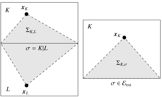
Figure 1: Construction of the dual cell $\Sigma_{K,L}$ between the cells $K,L$ and the dual cell $\Sigma_{K,\sigma}$ at the boundary of $\Omega$.

Definition 3.

Let $w\in\text{$\mathcal{H}$}^{\Pi}$. We define the piecewise constant interpolation operator $\mathcal{S}_{\Pi}:\text{$\mathcal{H}$}^{\Pi}\rightarrow\left\{f\left|f:\Omega\rightarrow\mathbb{R}\right.\right\}$ as

$$\left(\mathcal{S}_{\Pi}w\right)\left(\bm{x}\right)\equiv w\left(\bm{x}_{K}\right),\forall K\in\Pi,\forall\bm{x}\in K.$$

The piecewise linear interpolation $\mathcal{Q}_{\Pi}:\text{$\mathcal{H}$}^{\Pi}\rightarrow\left\{f\left|f:\Omega\rightarrow\mathbb{R}\right.\right\}$ is defined as

$$\left(\text{$\mathcal{Q}$}_{\Pi}w\right)\left(\bm{x}\right)\equiv w\left(\bm{x}_{K}\right)+\frac{1}{\left\|\bm{x}_{L}-\bm{x}_{K}\right\|^{2}}\left(\bm{x}-\bm{x}_{K}\right)\cdot\left(\bm{x}_{L}-\bm{x}_{K}\right)\left[w\left(\bm{x}_{L}\right)-w\left(\bm{x}_{K}\right)\right]$$

$$\forall\varSigma_{K,L}\in\Pi^{*},\bm{x}\in\varSigma_{K,L},$$

and

$$\left(\text{$\mathcal{Q}$}_{\Pi}w\right)\left(\bm{x}\right)\equiv w\left(\bm{x}_{K}\right)+\frac{1}{\left\|\bm{y}_{\sigma}-\bm{x}_{K}\right\|^{2}}\left(\bm{x}-\bm{x}_{K}\right)\cdot\left(\bm{y}_{\sigma}-\bm{x}_{K}\right)\left[-w\left(\bm{x}_{K}\right)\right]$$

$$\forall\varSigma_{K,\sigma}\in\Pi^{*},\bm{x}\in\varSigma_{K,\sigma}.$$

Definition 4.

For $v,w\in\text{$\mathcal{H}$}^{\Pi}$, we define

$$\left(v,w\right)_{\Pi} \equiv\underset{K\in\Pi}{\sum}m\left(K\right)v_{K}w_{K},$$

$$\left\|w\right\|_{\Pi} \equiv\sqrt{\left(w,w\right)_{\Pi}^{2}},$$

$$\left\llbracket w\right\rrbracket_{\Pi}^{2} \equiv\underset{{\sigma\in\text{$\mathcal{E}$}_{K}\cap\text{$\mathcal{E}$}_{\text{int}}\atop\sigma=K|L}}{\sum}\tau_{\sigma}\left(w_{K}-w_{L}\right)^{2}+\underset{{\sigma\in\text{$\mathcal{E}$}_{\text{ext}}\atop\sigma\in\mathcal{E}_{K}}}{\sum}\tau_{\sigma}w_{K}^{2}.$$

Lemma 1.

Let $v,w\in\text{$\mathcal{H}$}^{\Pi}$, then the relationships

$$\left(v,w\right)_{\Pi} =\left(\mathcal{S}_{\Pi}v,\mathcal{S}_{\Pi}w\right)_{\text{L}^{2}\left(\Omega\right)},$$ (27)

$$\left\|w\right\|_{\Pi}^{2} =\left\|\mathcal{S}_{\Pi}w\right\|_{\text{L}^{2}\left(\Omega\right)}^{2},$$ (28)

$$\left\llbracket w\right\rrbracket_{\Pi}^{2} =3\left\|\left|\nabla\mathcal{Q}_{\Pi}w\right|\right\|_{\text{L}^{2}\left(\Omega\right)}^{2}.$$ (29)

hold.

Proof.

(27) and (28) follow directly from the definition of the respective inner products. To prove (29), we recall Definition (3), relation (8), and the notations of Figure 2 so that we can write

$$\left\llbracket w\right\rrbracket_{\Pi}^{2} =\underset{{\sigma\in\text{$\mathcal{E}$}_{K}\cap\text{$\mathcal{E}$}_{\text{int}}\atop\sigma=K|L}}{\sum}\tau_{\sigma}\left(w_{K}-w_{L}\right)^{2}+\underset{{\sigma\in\text{$\mathcal{E}$}_{\text{ext}}\atop\sigma\in\mathcal{E}_{K}}}{\sum}\tau_{\sigma}w_{K}^{2}$$

$$=\underset{{\sigma\in\text{$\mathcal{E}$}_{K}\cap\text{$\mathcal{E}$}_{\text{int}}\atop\sigma=K|L}}{\sum}\frac{m\left(\sigma\right)}{d_{\sigma}}\left(w_{K}-w_{L}\right)^{2}+\underset{{\sigma\in\text{$\mathcal{E}$}_{\text{ext}}\atop\sigma\in\mathcal{E}_{K}}}{\sum}\frac{m\left(\sigma\right)}{d_{\sigma}}w_{K}^{2}$$

$$=\underset{{\sigma\in\text{$\mathcal{E}$}_{K}\cap\text{$\mathcal{E}$}_{\text{int}}\atop\sigma=K|L}}{\sum}m\left(\sigma\right)\left(d_{K,\sigma}+d_{L,\sigma}\right)\left(\frac{w_{K}-w_{L}}{d_{\sigma}}\right)^{2}+\underset{{\sigma\in\text{$\mathcal{E}$}_{\text{ext}}\atop\sigma\in\mathcal{E}_{K}}}{\sum}m\left(\sigma\right)d_{K,\sigma}\left(\frac{w_{K}}{d_{\sigma}}\right)^{2}$$

$$=\underset{{\sigma\in\text{$\mathcal{E}$}_{K}\cap\text{$\mathcal{E}$}_{\text{int}}\atop\sigma=K|L}}{\sum}m\left(\sigma\right)\left(d_{K,\sigma}+d_{L,\sigma}\right)\left|\nabla\mathcal{Q}_{\Pi}w\left(\bm{y}_{\sigma}\right)\right|^{2}$$

$$+\underset{{\sigma\in\text{$\mathcal{E}$}_{\text{ext}}\atop\sigma\in\mathcal{E}_{K}}}{\sum}m\left(\sigma\right)d_{K,\sigma}\left|\nabla\mathcal{Q}_{\Pi}w\left(\bm{y}_{\sigma}\right)\right|^{2}$$

$$=\sum_{K\in\Pi}\sum_{\sigma\in\mathcal{E}_{K}}m\left(\sigma\right)d_{K,\sigma}\left|\nabla\mathcal{Q}_{\Pi}w\left(\bm{y}_{\sigma}\right)\right|^{2}$$

$$=\sum_{K\in\Pi}\sum_{\sigma\in\mathcal{E}_{K}}3\int\limits_{\Sigma_{K,\sigma}}\left|\nabla\mathcal{Q}_{\Pi}w\left(\bm{x}\right)\right|^{2}\text{d}\bm{x}=3\int\limits_{\Omega}\nabla\mathcal{Q}_{\Pi}w\left(\bm{x}\right)\cdot\nabla\mathcal{Q}_{\Pi}w\left(\bm{x}\right)\text{d}\bm{x}$$

$$=3\left\|\left|\nabla\mathcal{Q}_{\Pi}w\right|\right\|_{\text{L}^{2}\left(\Omega\right)}^{2}.$$

∎

Lemma 2.

Let $\Pi$ be an admissible mesh. Then there exists a mesh dependent constant $C_{\Pi}>0$ such that for all $w\in\text{$\mathcal{H}$}^{\Pi}$, the inequality

$$\left\|\text{$\mathcal{Q}$}_{\Pi}w\right\|_{\text{L}^{2}\left(\Omega\right)}\leq C_{\Pi}\left\|\mathcal{S}_{\Pi}w\right\|_{\text{L}^{2}\left(\Omega\right)}$$ (30)

holds.

Proof.

Let $\Sigma_{K,L}\in\Pi^{*}$ be a cell of the dual mesh and denote $\sigma=K|L$. From Definition 3, we easily get

$$\left\|\text{$\mathcal{S}$}_{\Pi}w\right\|_{\text{L}^{2}\left(\varSigma_{K,L}\right)}^{2}=\frac{1}{3}\widetilde{m}\left(\sigma\right)\left(d_{K,\sigma}w_{K}^{2}+d_{L,\sigma}w_{L}^{2}\right).$$ (31)

To evaluate $\left\|\mathcal{Q}_{\Pi}w\right\|_{\text{L}^{2}\left(\varSigma_{K,L}\right)}^{2}$, we represent $\Sigma_{K,L}$ (see Figure 2

Figure 2: On the calculation of $\left\|\text{$\mathcal{Q}$}_{\Pi}u\right\|_{\text{L}^{2}\left(\varSigma_{K,L}\right)}^{2}$ on the dual cell $\Sigma_{K,L}$.

) in an affine space centered at $\bm{y}_{\sigma}$ with an orthonormal basis $V=\left(\bm{v}_{1},\bm{v}_{2},\bm{v}_{3}\right)$ where $\bm{v}_{1}=\frac{\bm{x}_{L}-\bm{x}_{K}}{\left|\bm{x}_{L}-\bm{x}_{K}\right|}$. The coordinates of a point $\bm{x}\in\Sigma_{K,L}$ in $V$ will be denoted by $\left(\alpha_{1},\alpha_{2},\alpha_{3}\right)$, i.e.

$$\bm{x}=\bm{y}_{\sigma}+\sum_{i=1}^{3}\alpha_{i}\bm{v}_{i}.$$

By means of this transformation, we have

$$\left\|\text{$\mathcal{Q}$}_{\Pi}w\right\|_{\text{L}^{2}\left(\varSigma_{K,L}\right)}^{2}=\int\limits_{-d_{K,\sigma}}^{d_{L,\sigma}}\text{d}\alpha_{1}\int\limits_{\tilde{S}\left(\alpha_{1}\right)}\text{d}\left(\alpha_{2},\alpha_{3}\right)\left[\left(\text{$\mathcal{Q}$}_{\Pi}w\right)\left(\bm{y}_{\sigma}+\sum_{i=1}^{3}\alpha_{i}\bm{v}_{i}\right)\right]^{2}$$ (32)

where

$$\tilde{S}\left(\alpha_{1}\right)=\left\{\left(\alpha_{2},\alpha_{3}\right)\in\mathbb{R}^{2};\bm{y}_{\sigma}+\sum_{i=1}^{3}\alpha_{i}\bm{v}_{i}\in\Sigma_{K,L}\right\}.$$

In addition, denote by $S\left(\alpha_{1}\right)$ the corresponding planar cut through $\Sigma_{K,L}$, i.e.

$$S\left(\alpha_{1}\right)=\left\{\bm{y}_{\sigma}+\sum_{i=1}^{3}\alpha_{i}\bm{v}_{i};\left(\alpha_{2},\alpha_{3}\right)\in\tilde{S}\left(\alpha_{1}\right)\right\}.$$

In (32), Definition 3 allows to evaluate

$$\left(\text{$\mathcal{Q}$}_{\Pi}w\right)\left(\bm{y}_{\sigma}+\sum_{i=1}^{3}\alpha_{i}\bm{v}_{i}\right)=w_{K}+\frac{\alpha_{1}+d_{K,\sigma}}{d_{L,\sigma}+d_{K,\sigma}}\left(w_{L}-w_{K}\right)$$ (33)

which only depends on $\alpha_{1}$. Next, the term $\int\limits_{\tilde{S}\left(\alpha_{1}\right)}\text{d}\left(\alpha_{2},\alpha_{3}\right)$ represents the surface area of $S\left(\alpha_{1}\right)$ which satisfies

$$\int\limits_{\tilde{S}\left(\alpha_{1}\right)}\text{d}\left(\alpha_{2},\alpha_{3}\right)=\tilde{m}\left(S\left(\alpha_{1}\right)\right)=\begin{cases}\tilde{m}\left(\sigma\right)\frac{d_{K,\sigma}+\alpha_{1}}{d_{K,\sigma}}&\alpha_{1}\in\left[-d_{K,\sigma},0\right],\\ \tilde{m}\left(\sigma\right)\frac{d_{L,\sigma}-\alpha_{1}}{d_{L,\sigma}}&\alpha_{1}\in\left[0,d_{L,\sigma}\right].\end{cases}$$ (34)

Plugging (33) and (34) into (32) and performing the integrationEXPLANATION: See the Lemma_Q-S.mw MAPLE worksheet with respect to $\alpha_{1}$ leads to

$$\left\|\text{$\mathcal{Q}$}_{\Pi}w\right\|_{\text{L}^{2}\left(\varSigma_{K,L}\right)}^{2} =\frac{1}{12}\frac{\tilde{m}\left(\sigma\right)}{d_{K,\sigma}+d_{L,\sigma}}\bigg{[}\left(d_{K,\sigma}^{2}+3d_{K,\sigma}d_{L,\sigma}+3d_{L,\sigma}^{2}\right)w_{K}^{2}$$

$$+2\left(d_{K,\sigma}^{2}+3d_{K,\sigma}d_{L,\sigma}+d_{L,\sigma}^{2}\right)w_{K}w_{L}$$

$$+\left(3d_{K,\sigma}^{2}+3d_{K,\sigma}d_{L,\sigma}+d_{L,\sigma}^{2}\right)w_{L}^{2}\bigg{]}.$$

By the Young inequality, this can be estimated as

$$\left\|\text{$\mathcal{Q}$}_{\Pi}w\right\|_{\text{L}^{2}\left(\varSigma_{K,L}\right)}^{2} \leq\frac{1}{6}\frac{\tilde{m}\left(\sigma\right)}{d_{K,\sigma}+d_{L,\sigma}}\bigg{[}\left(d_{K,\sigma}^{2}+3d_{K,\sigma}d_{L,\sigma}+2d_{L,\sigma}^{2}\right)w_{K}^{2}$$

$$+\left(2d_{K,\sigma}^{2}+3d_{K,\sigma}d_{L,\sigma}+d_{L,\sigma}^{2}\right)w_{L}^{2}\bigg{]}.$$

The equality (31) can be rewritten into a similar form

$$\left\|\mathcal{S}_{\Pi}w\right\|_{\text{L}^{2}\left(\varSigma_{K,L}\right)}^{2} =\frac{1}{6}\frac{\tilde{m}\left(\sigma\right)}{d_{K,\sigma}+d_{L,\sigma}}\bigg{[}\left(2d_{K,\sigma}^{2}+2d_{K,\sigma}d_{L,\sigma}\right)w_{K}^{2}$$

$$+\left(2d_{K,\sigma}d_{L,\sigma}+2d_{L,\sigma}^{2}\right)w_{L}^{2}\bigg{]}.$$

Defining

$$C_{K,L}\equiv\max\left\{\frac{d_{K,\sigma}^{2}+3d_{K,\sigma}d_{L,\sigma}+2d_{L,\sigma}^{2}}{2d_{K,\sigma}^{2}+2d_{K,\sigma}d_{L,\sigma}},\frac{2d_{K,\sigma}^{2}+3d_{K,\sigma}d_{L,\sigma}+d_{L,\sigma}^{2}}{2d_{K,\sigma}d_{L,\sigma}+2d_{L,\sigma}^{2}}\right\},$$

we observe that

$$\left\|\text{$\mathcal{Q}$}_{\Pi}w\right\|_{\text{L}^{2}\left(\varSigma_{K,L}\right)}^{2}\leq C_{K,L}\left\|\text{$\mathcal{S}$}_{\Pi}w\right\|_{\text{L}^{2}\left(\varSigma_{K,L}\right)}^{2}.$$

Note that $C_{K,L}$ is only dependent on the ratio between $d_{K,\sigma}$ and $d_{L,\sigma}$, not on their absolute values. Namely, it is independent of $w$ and of any mesh refinement as long as the geometry of the cells remains unchangedTODO: The note about mesh geometry can possibly be rewritten or omitted. .

An analogous inequality in the form

$$\left\|\text{$\mathcal{Q}$}_{\Pi}w\right\|_{\text{L}^{2}\left(\varSigma_{K,\sigma}\right)}^{2}\leq C_{K,\sigma}\left\|\text{$\mathcal{S}$}_{\Pi}w\right\|_{\text{L}^{2}\left(\varSigma_{K,\sigma}\right)}^{2}$$

can be derived for the dual cells $\Sigma_{K,\sigma}$ at the boundary of $\Omega$.NOTE: It is also possible to mirror $\Sigma_{K,\sigma}$ along $\sigma$ to obtain a “ghost” cell $L$ with $w_{L}=-w_{K}$ which ensures that $\left(\mathcal{Q}w\right)\left(\bm{y}_{\sigma}\right)=0$. Then we perform the procedure exactly as shown above and the resulting norms are just $\frac{1}{2}$ of the obtained values. Define

$$C_{\Pi}\equiv\text{max}\left(\left\{C_{K,L};K|L\in\text{$\mathcal{E}$}_{\text{int}}\right\}\cup\left\{C_{K,\sigma};\sigma\in\text{$\mathcal{E}$}_{\text{ext}}\right\}\right).$$

Summing up the estimates

$$\left\|\text{$\mathcal{Q}$}_{\Pi}w\right\|_{\text{L}^{2}\left(\varSigma_{K,L}\right)}^{2}\leq C_{\Pi}\left\|\text{$\mathcal{S}$}_{\Pi}w\right\|_{\text{L}^{2}\left(\varSigma_{K,L}\right)}^{2},$$

$$\left\|\text{$\mathcal{Q}$}_{\Pi}w\right\|_{\text{L}^{2}\left(\varSigma_{K,\sigma}\right)}^{2}\leq C_{\Pi}\left\|\text{$\mathcal{S}$}_{\Pi}w\right\|_{\text{L}^{2}\left(\varSigma_{K,\sigma}\right)}^{2}$$

over all cells of the dual mesh concludes the proof. ∎

5 Convergence

The existence, uniqueness of the weak solution and convergence of the numerical scheme will be shown using a single procedure that relies on an a priori estimate to ensure boundedness of the respective numerical solutions. This estimate is independent of mesh refinement. The procedure uses and expands upon some of the ideas presented in [11] and [10]. For the sake of simplicity, the homogeneous Dirichlet boundary conditions

$$\begin{array}[]{c}u_{\partial\Omega}=0,\end{array} \text{ }p_{\partial\Omega}=0$$ (36)

are considered, allowing to simplify (21) and (22) to

$$F_{K,\sigma}\left(w_{\Pi}\right) \equiv F_{K,\sigma}\left(w_{\Pi},0\right),\quad F_{K}\left(w_{\Pi}\right)\equiv F_{K}\left(w_{\Pi},0\right),$$

$$F\left(w_{\Pi}\right) \equiv F\left(w_{\Pi},0\right)\qquad\forall w\in\text{$\mathcal{H}$}^{\Pi}$$

5.1 Weak Formulation

Testing the equations (1)–(2) by $\psi$, $\varphi\in\text{C}_{0}^{\infty}\left(\mathcal{J}\right)$ and $v$, $q\in\text{C}_{0}^{\infty}\left(\Omega\right)$, the weak formulation

$$\stackrel{{\scriptstyle[}}{{0}}]{T}{\int}\frac{\text{d}}{\text{d}t}\underset{\Omega}{\int}u\left(t,\bm{x}\right)v\left(\bm{x}\right)\text{d}\bm{x}\psi\left(t\right)\text{d}t +\stackrel{{\scriptstyle[}}{{0}}]{T}{\int}\underset{\Omega}{\int}\nabla u\left(t,\bm{x}\right)\cdot\nabla v\left(\bm{x}\right)\text{d}\bm{x}\psi\left(t\right)\text{d}t$$

$$=\stackrel{{\scriptstyle[}}{{0}}]{T}{\int}\frac{\text{d}}{\text{d}t}\underset{\Omega}{\int}Lp\left(t,\bm{x}\right)v\left(\bm{x}\right)\text{d}\bm{x}\psi\left(t\right)\text{d}t,$$ (37)

$$\alpha\xi^{2}\stackrel{{\scriptstyle[}}{{0}}]{T}{\int}\frac{\text{d}}{\text{d}t}\underset{\Omega}{\int}p\left(t,\bm{x}\right)q\left(\bm{x}\right)\text{d}\bm{x}\varphi\left(t\right)\text{d}t +\xi^{2}\stackrel{{\scriptstyle[}}{{0}}]{T}{\int}\underset{\Omega}{\int}\nabla p\left(t,\bm{x}\right)\cdot\nabla q\left(\bm{x}\right)\text{d}\bm{x}\varphi\left(t\right)\text{d}t$$

$$=\stackrel{{\scriptstyle[}}{{0}}]{T}{\int}\underset{\Omega}{\int}f\left(u,p,\nabla p;\xi\right)q\left(\bm{x}\right)\text{d}\bm{x}\varphi\left(t\right)\text{d}t,$$ (38)

arises, completed by the initial conditions

$$u\mid_{t=0}=u_{\text{ini}},p\mid_{t=0}=p_{\text{ini}}.$$

Definition 5.

A pair of functions $\left(u,p\right)$, such that $u\in\text{L}^{2}\left(\text{$\mathcal{J}$};\text{H}_{0}^{1}\left(\Omega\right)\right),p\in\text{L}^{2}\left(\text{$\mathcal{J}$};\text{H}_{0}^{1}\left(\Omega\right)\right)$ that satisfy (37)–(38) with the initial conditions (3) for all $\psi,\varphi\in\text{C}_{0}^{\infty}\left(\mathcal{J}\right)$ and all $v,q\in\text{C}_{0}^{\infty}\left(\Omega\right)$ is called the weak solution of the problem (1)–(3) with the boundary conditions (36).

5.2 A priori Estimates

Let $\Pi$ be an admissible mesh. Consider the semi-discrete scheme (23), (24). Multiplying equation (23) by $\dot{u}_{K}\left(t\right)$ and equation (24) by $\dot{p}_{K}\left(t\right)$ respectively, summing each of them over all $K\in\Pi$ and using the definition of $\left(u,v\right)_{\Pi}$ yields

$$\left\|\dot{u}_{\Pi}\left(t\right)\right\|_{\Pi}^{2}+\left(F\left(u_{\Pi}\left(t\right)\right),\dot{u}_{\Pi}\left(t\right)\right)_{\Pi} =L\left(\dot{p}_{\Pi}\left(t\right),\dot{u}_{\Pi}\left(t\right)\right)_{\Pi},$$ (39)

$$\alpha\xi^{2}\left\|\dot{p}_{\Pi}\left(t\right)\right\|_{\Pi}^{2}+\xi^{2}\left(F\left(p_{\Pi}\left(t\right)\right),\dot{p}_{\Pi}\left(t\right)\right)_{\Pi} =\overbrace{\underset{K\in\Pi}{\sum}m\left(K\right)f_{0}\left(p_{K}\left(t\right)\right)\dot{p}_{K}\left(t\right)}^{\text{I}.}$$ (40)

$$-b\beta\xi\left(\varLambda_{\Pi}\left(t\right),\dot{p}_{K}\left(t\right)\right)_{\Pi}.$$

Using the chain rule and the fact that $f_{0}$ is the derivative of the double well potential $w_{0}$ (see [16, 11] and the proof of Lemma 3), we obtain

$$f_{0}\left(p\left(t\right)\right)\dot{p}_{K}\left(t\right)=-\frac{\text{d}w_{0}}{\text{d}t}\left(p_{K}(t)\right).$$ (41)

Rewriting expression I. using (41), we get

$$\underset{K\in\Pi}{\sum}m\left(K\right)f_{0}\left(p_{K}\left(t\right)\right)\dot{p}_{K}\left(t\right) =\underset{K\in\Pi}{\sum}-\frac{\text{d}w_{0}}{\text{d}t}\left(p_{K}(t)\right)m(K).$$ (42)

The Schwarz and Young inequalities applied on the right hand side of (39) and (40) together with the boundedness of $\Lambda$ (bounded by the constant $B$) and (42) give

$$\frac{1}{2}\left\|\dot{u}_{\Pi}\left(t\right)\right\|_{\Pi}^{2}+\left(F\left(u_{\Pi}\left(t\right)\right),\dot{u}_{\Pi}\left(t\right)\right)_{\Pi} \leq\frac{L^{2}}{2}\left\|\dot{p}_{\Pi}\left(t\right)\right\|_{\Pi}^{2},$$ (43)

$$\frac{1}{2}\alpha\xi^{2}\left\|\dot{p}_{\Pi}\left(t\right)\right\|_{\Pi}^{2}+\xi^{2}\left(F\left(p_{\Pi}\left(t\right)\right),\dot{p}_{\Pi}\left(t\right)\right)_{\Pi} +\frac{\text{d}}{\text{d}t}\underset{K\in\Pi}{\sum}w_{0}\left(p_{K}(t)\right)m(K)$$ (44)

$$\leq \frac{\left(b\beta\right)^{2}}{2\alpha}B^{2}m\left(\Omega\right).$$

Multiplying (43) by $\frac{\alpha\xi^{2}}{2\text{L}^{2}}$ and adding it to (44) results in a single inequality

$$\frac{1}{4}\alpha\xi^{2}\left\|\dot{p}_{\Pi}\left(t\right)\right\|_{\Pi}^{2}+\frac{1}{4}\frac{\alpha\xi^{2}}{2\text{L}^{2}}\left\|\dot{u}_{\Pi}\left(t\right)\right\|_{\Pi}^{2} +\xi^{2}\overbrace{\left(F\left(p_{\Pi}\left(t\right)\right),\dot{p}_{\Pi}\left(t\right)\right)_{\Pi}}^{\text{I.}}$$ (45)

$$+\frac{\alpha\xi^{2}}{2\text{L}^{2}}\overbrace{\left(F\left(u_{\Pi}\left(t\right)\right),\dot{u}_{\Pi}\left(t\right)\right)_{\Pi}}^{\text{II.}}+\frac{\text{d}}{\text{d}t}\underset{K\in\Pi}{\sum}w_{0}\left(p_{K}(t)\right)m(K) \leq\frac{\left(b\beta\right)^{2}}{2\alpha}B^{2}m\left(\Omega\right).$$

We reformulate the terms I. and II. Under the assumption (36), the term I. can be rewritten by summation over faces $\sigma\in\mathcal{E}$ instead of cells $K\in\Pi$ as follows

$$\text{I.}= \underset{K\in\Pi}{\sum}\left(\underset{\sigma\in\text{$\mathcal{E}$}_{K}}{\sum}F_{K,\sigma}\left(p_{\Pi}\left(t\right)\right)\right)\dot{p}_{\Pi}\left(t\right)$$ (46)

$$= \underset{K\in\Pi}{\sum}\underset{{\sigma\in\text{$\mathcal{E}$}_{K}\cap\text{$\mathcal{E}$}_{\text{int}}\atop\sigma=K|L}}{\sum}-\tau_{\sigma}\left(p_{L}\left(t\right)-p_{K}\left(t\right)\right)\dot{p}_{k}\left(t\right)$$

$$+ \underset{K\in\Pi}{\sum}\underset{\sigma\in\text{$\mathcal{E}$}_{K}\cap\text{$\mathcal{E}$}_{\text{ext}}}{\sum}-\tau_{\sigma}\left(-p_{K}\left(t\right)\right)\dot{p}_{k}\left(t\right)$$

$$= -\underset{{\sigma\in\text{$\mathcal{E}$}_{\text{int}}\atop\sigma=K\left|L\right.}}{\sum}\tau_{\sigma}\left[\left(p_{L}\left(t\right)-p_{K}\left(t\right)\right)\dot{p}_{K}\left(t\right)+\left(p_{K}\left(t\right)-p_{L}\left(t\right)\right)\dot{p}_{L}\left(t\right)\right]$$

$$+ \underset{{\sigma\in\text{$\mathcal{E}$}_{\text{ext}}\atop\sigma\in\mathcal{E}_{K}}}{\sum}\tau_{\sigma}p_{K}\left(t\right)\dot{p}_{K}\left(t\right)$$

$$= \frac{1}{2}\underset{{\sigma\in\text{$\mathcal{E}$}_{\text{int}}\atop\sigma=K\left|L\right.}}{\sum}\tau_{\sigma}\left[\frac{\text{d}}{\text{d}t}\left(p_{K}\left(t\right)\right)^{2}-2\frac{\text{d}}{\text{d}t}\left(p_{L}\left(t\right)p_{K}\left(t\right)\right)+\frac{\text{d}}{\text{d}t}\left(p_{L}\left(t\right)\right)^{2}\right]$$

$$+ \frac{1}{2}\underset{{\sigma\in\text{$\mathcal{E}$}_{\text{ext}}\atop\sigma\in\mathcal{E}_{K}}}{\sum}\tau_{\sigma}\frac{\text{d}}{\text{d}t}\left(p_{K}\left(t\right)\right)^{2}$$

$$= \frac{1}{2}\frac{\text{d}}{\text{d}t}\underset{{\sigma\in\text{$\mathcal{E}$}_{\text{int}}\atop\sigma=K\left|L\right.}}{\sum}\tau_{\sigma}\left[p_{K}\left(t\right)-p_{L}\left(t\right)\right]^{2}+\frac{1}{2}\frac{\text{d}}{\text{d}t}\underset{{\sigma\in\text{$\mathcal{E}$}_{\text{ext}}\atop\sigma\in\mathcal{E}_{K}}}{\sum}\tau_{\sigma}\left(p_{K}\left(t\right)\right)^{2}.$$

An analogous calculation performed on term II. together with Definition 4 give

$$\text{I.}=\frac{1}{2}\frac{\text{d}}{\text{d}t}\left\llbracket u_{\Pi}\left(t\right)\right\rrbracket_{\Pi}^{2},\qquad\text{II.}=\frac{1}{2}\frac{\text{d}}{\text{d}t}\left\llbracket p_{\Pi}\left(t\right)\right\rrbracket_{\Pi}^{2}.$$ (47)

The identities (47) make it possible to write (45) in the form

$$\frac{1}{4}\alpha\xi^{2}\left\|\dot{p}_{\Pi}\left(t\right)\right\|_{\Pi}^{2}+\frac{1}{4}\frac{\alpha\xi^{2}}{2\text{L}^{2}}\left\|\dot{u_{\Pi}}\left(t\right)\right\|_{\Pi}^{2}+\frac{1}{2}\xi^{2}\frac{\text{d}}{\text{d}t}\left\llbracket p_{\Pi}\left(t\right)\right\rrbracket_{\Pi}^{2}$$

$$+ \frac{1}{2}\frac{\alpha\xi^{2}}{2\text{L}^{2}}\frac{\text{d}}{\text{d}t}\left\llbracket u_{\Pi}\left(t\right)\right\rrbracket_{\Pi}^{2}+\frac{\text{d}}{\text{d}t}\underset{K\in\Pi}{\sum}w_{0}\left(p_{K}(t)\right)m(K)$$ (48)

$$\leq \frac{\left(b\beta\right)^{2}}{2\alpha}B^{2}m\left(\Omega\right).$$

At this point, the inequality (48) will be used in two different ways. The first result will be used within the derivation of the second to obtain the final estimate. First, the nonnegative terms $\left\|\dot{p}_{\Pi}\left(t\right)\right\|_{\Pi}^{2}$ and $\left\|\dot{u_{\Pi}}\left(t\right)\right\|_{\Pi}^{2}$ are omitted from the left hand side of (48) and the nonnegative expression

$$\xi^{2}\frac{1}{2}\left\llbracket p_{\Pi}\left(t\right)\right\rrbracket_{\Pi}^{2}+\frac{1}{2}\frac{\alpha\xi^{2}}{2\text{L}^{2}}\left\llbracket u_{\Pi}\left(t\right)\right\rrbracket_{\Pi}^{2}+\underset{K\in\Pi}{\sum}w_{0}\left(p_{K}(t)\right)m(K)$$ (49)

is added to the right hand side of (48), giving rise to

$$\frac{1}{2}\xi^{2}\frac{\text{d}}{\text{d}t}\left\llbracket p_{\Pi}\left(t\right)\right\rrbracket_{\Pi}^{2}+\frac{1}{2}\frac{\alpha\xi^{2}}{2\text{L}^{2}}\frac{\text{d}}{\text{d}t}\left\llbracket u_{\Pi}\left(t\right)\right\rrbracket_{\Pi}^{2}+\frac{\text{d}}{\text{d}t}\underset{K\in\Pi}{\sum}w_{0}\left(p_{K}(t)\right)m(K)$$

$$\leq \xi^{2}\frac{1}{2}\left\llbracket p_{\Pi}\left(t\right)\right\rrbracket_{\Pi}^{2}+\frac{1}{2}\frac{\alpha\xi^{2}}{2\text{L}^{2}}\left\llbracket u_{\Pi}\left(t\right)\right\rrbracket_{\Pi}^{2}+\underset{K\in\Pi}{\sum}w_{0}\left(p_{K}(t)\right)m(K)$$

$$+ \frac{\left(b\beta\right)^{2}}{2\alpha}m\left(\Omega\right)B^{2}.$$ (50)

Let $s\in\mathbb{\text{$\mathcal{J}$}}$. Substituting $t$ for $s$, multiplying the whole inequality by $\text{e}^{-s}$ leads to

$$\frac{\text{d}}{\text{d}s}\left[\left(\frac{1}{2}\xi^{2}\left\llbracket p_{\Pi}\left(s\right)\right\rrbracket_{\Pi}^{2}+\frac{\alpha\xi^{2}}{4L}\left\llbracket u_{\Pi}\left(s\right)\right\rrbracket_{\Pi}^{2}+\underset{K\in\Pi}{\sum}w_{0}\left(p_{K}(s)\right)m(K)\right)\text{e}^{-s}\right]$$

$$\leq\frac{\left(b\beta\right)^{2}}{2\alpha}B^{2}m\left(\Omega\right)\text{e}^{-s}.$$

Integrating with respect to $s$ over $\left(0,t\right)$ gives

$$\frac{1}{2}\xi^{2}\left\llbracket p_{\Pi}\left(t\right)\right\rrbracket_{\Pi}^{2}+\frac{\alpha\xi^{2}}{4L}\left\llbracket u_{\Pi}\left(t\right)\right\rrbracket_{\Pi}^{2}+\underset{K\in\Pi}{\sum}w_{0}\left(p_{K}(t)\right)m(K)$$

$$\leq \left(\frac{1}{2}\xi^{2}\left\llbracket p_{\Pi}\left(0\right)\right\rrbracket_{\Pi}^{2}+\frac{\alpha\xi^{2}}{4L}\left\llbracket u_{\Pi}\left(0\right)\right\rrbracket_{\Pi}^{2}\right)\text{e}^{t}+\left(\underset{K\in\Pi}{\sum}w_{0}\left(p_{K}(0)\right)m(K)\right)\text{e}^{t}$$

$$+ \frac{\left(b\beta\right)^{2}}{2\alpha}B^{2}m\left(\Omega\right)\left(\text{e}^{t}-1\right).$$ (51)

This inequality will be used as part of the next estimate.

Revisiting (48) and adding the nonnegative expression (49) to the right hand side yields

$$\frac{1}{4}\alpha\xi^{2}\left\|\dot{p}_{\Pi}\left(t\right)\right\|_{\Pi}^{2}+\frac{1}{4}\frac{\alpha\xi^{2}}{2\text{L}^{2}}\left\|\dot{u}_{\Pi}\left(t\right)\right\|_{\Pi}^{2}$$ (52)

$$+ \frac{1}{2}\frac{\text{d}}{\text{d}t}\left(\xi^{2}\left\llbracket p_{\Pi}\left(t\right)\right\rrbracket_{\Pi}^{2}\right)+\frac{1}{2}\frac{\text{d}}{\text{d}t}\left(\frac{\alpha\xi^{2}}{2\text{L}^{2}}\left\llbracket u_{\Pi}\left(t\right)\right\rrbracket_{\Pi}^{2}\right)+\frac{\text{d}}{\text{d}t}\underset{K\in\Pi}{\sum}w_{0}\left(p_{K}(t)\right)m(K)$$

$$\leq \frac{\left(b\beta\right)^{2}}{2\alpha}B^{2}m\left(\Omega\right)+\frac{1}{2}\xi^{2}\left\llbracket p_{\Pi}\left(t\right)\right\rrbracket_{\Pi}^{2}$$

$$+ \frac{1}{2}\frac{\alpha\xi^{2}}{2\text{L}^{2}}\left\llbracket u_{\Pi}\left(t\right)\right\rrbracket_{\Pi}^{2}+\underset{K\in\Pi}{\sum}w_{0}\left(p_{K}(t)\right)m(K).$$

Integrating this estimate with respect to $t$ over $\text{$\mathcal{J}$}=\left(0,T\right)$ gives

$$\stackrel{{\scriptstyle[}}{{0}}]{T}{\int}\frac{1}{4}\alpha\xi^{2}\left\|\dot{p}_{\Pi}\left(t\right)\right\|_{\Pi}^{2}\text{d}t+\stackrel{{\scriptstyle[}}{{0}}]{T}{\int}\frac{1}{4}\frac{\alpha\xi^{2}}{2\text{L}^{2}}\left\|\dot{u}_{\Pi}\left(t\right)\right\|_{\Pi}^{2}\text{d}t+\frac{1}{2}\xi^{2}\left\llbracket p_{\Pi}\left(T\right)\right\rrbracket_{\Pi}^{2}$$

$$+ \frac{1}{2}\frac{\alpha\xi^{2}}{2\text{L}^{2}}\left\llbracket u_{\Pi}\left(T\right)\right\rrbracket_{\Pi}^{2}+\left(\underset{K\in\Pi}{\sum}w_{0}\left(p_{K}(T)\right)m(K)\right)$$

$$\leq \frac{1}{2}\xi^{2}\left\llbracket p_{\Pi}\left(0\right)\right\rrbracket_{\Pi}^{2}+\frac{1}{2}\frac{\alpha\xi^{2}}{2\text{L}^{2}}\left\llbracket u_{\Pi}\left(0\right)\right\rrbracket_{\Pi}^{2}$$

$$+ \stackrel{{\scriptstyle[}}{{0}}]{T}{\int}\frac{1}{2}\xi^{2}\left\llbracket p_{\Pi}\left(t\right)\right\rrbracket_{\Pi}^{2}+\frac{1}{2}\frac{\alpha\xi^{2}}{2\text{L}^{2}}\left\llbracket u_{\Pi}\left(t\right)\right\rrbracket_{\Pi}^{2}\text{d}t+\left(\underset{K\in\Pi}{\sum}w_{0}\left(p_{K}(0)\right)m(K)\right)$$

$$+ \stackrel{{\scriptstyle[}}{{0}}]{T}{\int}\underset{K\in\Pi}{\sum}w_{0}\left(p_{K}(t)\right)m(K)\text{d}t+\frac{\left(b\beta\right)^{2}}{2\alpha}B^{2}m\left(\Omega\right)T.$$ (53)

The relationship (51) is used to estimate the integral on the right hand side

$$\stackrel{{\scriptstyle[}}{{0}}]{T}{\int}\frac{1}{2}\xi^{2}\left\llbracket p_{\Pi}\left(t\right)\right\rrbracket_{\Pi}^{2}+\frac{1}{2}\frac{\alpha\xi^{2}}{2\text{L}^{2}}\left\llbracket u_{\Pi}\left(t\right)\right\rrbracket_{\Pi}^{2}\text{d}t+\stackrel{{\scriptstyle[}}{{0}}]{T}{\int}\underset{K\in\Pi}{\sum}w_{0}\left(p_{K}(t)\right)m(K)\text{d}t$$

$$\leq \stackrel{{\scriptstyle[}}{{0}}]{T}{\int}\left\{\frac{1}{2}\xi^{2}\left\llbracket p_{\Pi}\left(0\right)\right\rrbracket_{\Pi}^{2}\text{e}^{t}\right.+\frac{1}{2}\frac{\alpha\xi^{2}}{2\text{L}^{2}}\left\llbracket u_{\Pi}\left(0\right)\right\rrbracket_{\Pi}^{2}\text{e}^{t}$$

$$+ \left(\underset{K\in\Pi}{\sum}w_{0}\left(p_{K}(0)\right)m(K)\right)\text{e}^{t}+\left.\frac{\left(b\beta\right)^{2}}{2\alpha}B^{2}m\left(\Omega\right)\left(\text{e}^{t}-1\right)\right\}\text{d}t$$

$$= \left\{\frac{1}{2}\xi^{2}\left\llbracket p_{\Pi}\left(0\right)\right\rrbracket_{\Pi}^{2}\right.+\frac{1}{2}\frac{\alpha\xi^{2}}{2\text{L}^{2}}\left\llbracket u_{\Pi}\left(0\right)\right\rrbracket_{\Pi}^{2}$$

$$+ \left(\underset{K\in\Pi}{\sum}w_{0}\left(p_{K}(0)\right)m(K)\right)+\left.\frac{\left(b\beta\right)^{2}}{2\alpha}B^{2}m\left(\Omega\right)\right\}\left(\text{e}^{T}-1\right)-\frac{\left(b\beta\right)^{2}}{2\alpha}B^{2}m\left(\Omega\right)T.$$

Using this estimate to simplify the right hand side of (53) results in

$$\stackrel{{\scriptstyle[}}{{0}}]{T}{\int}\frac{1}{4}\alpha\xi^{2}\left\|\dot{p}_{\Pi}\left(t\right)\right\|_{\Pi}^{2}\text{d}t+\stackrel{{\scriptstyle[}}{{0}}]{T}{\int}\frac{1}{4}\frac{\alpha\xi^{2}}{2\text{L}^{2}}\left\|\dot{u}_{\Pi}\left(t\right)\right\|_{\Pi}^{2}\text{d}t+\frac{1}{2}\xi^{2}\left\llbracket p_{\Pi}\left(T\right)\right\rrbracket_{\Pi}^{2}$$

$$+ \frac{1}{2}\frac{\alpha\xi^{2}}{2\text{L}^{2}}\left\llbracket u_{\Pi}\left(T\right)\right\rrbracket_{\Pi}^{2}+\left(\underset{K\in\Pi}{\sum}w_{0}\left(p_{K}(T)\right)m(K)\right)$$

$$\leq \left[\frac{1}{2}\xi^{2}\left\llbracket p_{\Pi}\left(0\right)\right\rrbracket_{\Pi}^{2}+\frac{\alpha\xi^{2}}{2\text{L}^{2}}\left\llbracket u_{\Pi}\left(0\right)\right\rrbracket_{\Pi}^{2}+\left(\underset{K\in\Pi}{\sum}w_{0}\left(p_{K}(0)\right)m(K)\right)\right]\text{e}^{T}$$

$$+ \frac{\left(b\beta\right)^{2}}{2\alpha}B^{2}m\left(\Omega\right)\left(\text{e}^{T}-1\right).$$ (54)

Lemma 3.

There exists a constant $c_{w}>0$ such that

$$w_{0}\left(x\right)+c_{w}\geq x^{2}\qquad\forall x\in\mathbb{R}.$$ (55)

Proof.

Consider the relationship between $f_{0}$ and $w_{0}$

$$w_{0}\left(x\right)=-\stackrel{{\scriptstyle[}}{{0}}]{x}{\int}f_{0}\left(s\right)\text{d}s=\frac{1}{4}x^{2}\left(x-1\right)^{2}.$$

We rewrite the expression

$$w_{0}\left(x\right)-x^{2}=\frac{1}{4}x^{2}\left[\left(x-1\right)^{2}-4\right]=\frac{1}{4}x^{2}\left(x+1\right)\left(x-3\right),$$ (56)

which shows that for any $x>3$ or $x<-1$, (56) is positive. Hence the inequality (55) holds for any $c_{w}\geq 0$ when $x\in\left(-\infty,-1\right)\cup\left(3,+\infty\right)$. We extend this inequality to any $x\in\mathbb{R}$ by setting

$$c_{w}\equiv-\underset{x\in\left[-1,3\right]}{\text{min}}\frac{1}{4}x^{2}\left(x+1\right)\left(x-3\right).$$

∎

We apply Lemma 3 by estimating

$$\underset{K\in\Pi}{\sum}w_{0}\left(p_{K}(t)\right)m(K) \geq\underset{K\in\Pi}{\sum}p_{K}^{2}(t)m(K)-\left(c_{w},1\right)_{\Pi}$$

$$=\left\|\left(p_{\Pi}\left(t\right)\right)\right\|_{\Pi}^{2}-\left(c_{w},1\right)_{\Pi}$$

$$\geq-\left(c_{w},1\right)_{\Pi}.$$ (57)

Using (57) and Lemma 1, the estimate (54) can be rewritten as

$$\stackrel{{\scriptstyle[}}{{0}}]{T}{\int}\frac{1}{4}\alpha\xi^{2}\left\|\text{$\mathcal{S}$}_{\Pi}\dot{p}_{\Pi}\left(t\right)\right\|_{\text{L}^{2}\left(\Omega\right)}^{2}\text{d}t+\stackrel{{\scriptstyle[}}{{0}}]{T}{\int}\frac{1}{4}\frac{\alpha\xi^{2}}{2\text{L}^{2}}\left\|\text{$\mathcal{S}$}_{\Pi}\dot{u}_{\Pi}\left(t\right)\right\|_{\text{L}^{2}\left(\Omega\right)}^{2}\text{d}t$$

$$+ \frac{3}{2}\xi^{2}\left\|\left|\nabla\mathcal{Q}_{\Pi}p_{\Pi}\left(T\right)\right|\right\|_{\text{L}^{2}\left(\Omega\right)}^{2}+\frac{3}{2}\frac{\alpha\xi^{2}}{2\text{L}^{2}}\left\|\left|\nabla\mathcal{Q}_{\Pi}u_{\Pi}\right|\right\|_{\text{L}^{2}\left(\Omega\right)}^{2}$$

$$\leq \left[\frac{1}{2}\xi^{2}\left\llbracket p_{\Pi}\left(0\right)\right\rrbracket_{\Pi}^{2}+\frac{\alpha\xi^{2}}{2\text{L}^{2}}\left\llbracket u_{\Pi}\left(0\right)\right\rrbracket_{\Pi}^{2}+\left(\underset{K\in\Pi}{\sum}w_{0}\left(p_{K}(0)\right)m(K)\right)\right]\text{e}^{T}$$ (58)

$$+ \frac{\left(b\beta\right)^{2}}{2\alpha}B^{2}m\left(\Omega\right)\left(\text{e}^{T}-1\right)+\left(c_{w},1\right)_{\Pi}.$$

5.3 Convergence of the Numerical Solution

All the quantities on the left hand side of (58) are nonnegative, thus the left hand side is bounded from below. The estimate (58) shows that the left hand side is also bounded from above. This implies that all of the expressions on the left hand side of (58) are bounded. Interpreting this boundedness in the context of Bochner spaces, we get

$$\frac{\partial}{\partial t}\text{$\mathcal{S}$}_{\Pi}p_{\Pi} =\text{$\mathcal{S}$}_{\Pi}\dot{p}_{\Pi}\in\text{L}^{2}\left(\text{$\mathcal{J}$};\text{L}^{2}\left(\Omega\right)\right),$$ (59)

$$\frac{\partial}{\partial t}\text{$\mathcal{S}$}_{\Pi}u_{\Pi} =\text{$\mathcal{S}$}_{\Pi}\dot{u}_{\Pi}\in\text{L}^{2}\left(\text{$\mathcal{J}$};\text{L}^{2}\left(\Omega\right)\right).$$ (60)

Furthermore, using Lemma 2, it also holds that

$$\frac{\partial}{\partial t}\text{$\mathcal{Q}$}_{\Pi}p_{\Pi} \in\text{L}^{2}\left(\text{$\mathcal{J}$};\text{L}^{2}\left(\Omega\right)\right),$$

$$\frac{\partial}{\partial t}\text{$\mathcal{Q}$}_{\Pi}u_{\Pi} \in\text{L}^{2}\left(\text{$\mathcal{J}$};\text{L}^{2}\left(\Omega\right)\right).$$

The finite Bochner norms together with the boundedness of $\Omega$ and $\mathcal{J}$ imply essential boundednessAles: Extra proof 1 (??)

$$\text{$\mathcal{S}$}_{\Pi}p_{\Pi}\in L^{\infty}\left(\text{$\mathcal{J}$};\text{L}^{2}\left(\Omega\right)\right) ,\text{$\mathcal{Q}$}_{\Pi}p_{\Pi}\in L^{\infty}\left(\text{$\mathcal{J}$};\text{L}^{2}\left(\Omega\right)\right),$$

$$\text{$\mathcal{S}$}_{\Pi}u_{\Pi}\in L^{\infty}\left(\text{$\mathcal{J}$};\text{L}^{2}\left(\Omega\right)\right), \text{$\mathcal{Q}$}_{\Pi}u_{\Pi}\in L^{\infty}\left(\text{$\mathcal{J}$};\text{L}^{2}\left(\Omega\right)\right).$$

Finally, the estimate (58) also givesOMITTED:

$$\frac{\partial}{\partial x^{i}}\text{$\mathcal{Q}$}_{\Pi}p_{\Pi} \in L^{\infty}\left(\text{$\mathcal{J}$};\text{L}^{2}\left(\Omega\right)\right),i\in\left\{1,2,3\right\},$$

$$\frac{\partial}{\partial x^{i}}\text{$\mathcal{Q}$}_{\Pi}u_{\Pi} \in L^{\infty}\left(\text{$\mathcal{J}$};\text{L}^{2}\left(\Omega\right)\right),i\in\left\{1,2,3\right\}.$$

$$\text{$\mathcal{Q}$}_{\Pi}p_{\Pi} \in L^{\infty}\left(\text{$\mathcal{J}$};\text{H}_{0}^{1}\left(\Omega\right)\right),$$ (61)

$$\text{$\mathcal{Q}$}_{\Pi}u_{\Pi} \in L^{\infty}\left(\text{$\mathcal{J}$};\text{H}_{0}^{1}\left(\Omega\right)\right).$$ (62)

In order to facilitate the subsequent analysis, we introduce the concept of a normal sequence of meshes.

Definition 6.

The norm of an admissible mesh $\Pi$ is defined as

$$\left|\Pi\right|\equiv\underset{K\in\Pi}{\text{max}}\,\text{$\inf$}\left\{r>0\left|\exists x_{0}\in\mathbb{R}^{3}:\forall x\in K:\left|x-x_{0}\right|<r\right.\right\}.$$

A sequence of admissible meshes $\left(\Pi_{n}\right)$ is called normal if and only if $\underset{n\rightarrow+\infty}{\text{lim}}\left|\Pi_{n}\right|=0$.This is our “original” term based on the normal sequence of partitions in the construction of Riemann integral.

Lemma 4.

Let $w\in\text{L}^{2}\left(\Omega\right)$ and $\Pi_{n}$ be a normal sequence of admissible meshes. Then

$$\text{$\mathcal{S}$}_{\Pi_{n}}\text{$\mathcal{P}$}_{\Pi_{n}}w\rightarrow w\text{ in }\text{L}^{2}\left(\Omega\right).$$ (63)

Lemma 4 is a consequence of the definition of the operators $\text{$\mathcal{S}$}_{\Pi_{n}},\text{$\mathcal{P}$}_{\Pi_{n}}$, and Lebesgue integration theory [32].

Lemma 5.

Let $u_{\text{ini}},p_{\text{ini}}\in\text{C}^{2}\left(\Omega\right)$ and let $\left(\Pi_{n}\right)$ be a normal sequence of admissible meshes. Then there exists an increasing sequence $\left(k_{n}\right)\subset\mathbb{N}$ and functions $p,u\in\text{L}^{2}\left(\text{$\mathcal{J}$};\text{H}_{0}^{1}\left(\Omega\right)\right)$ with the derivatives $\frac{\partial p}{\partial t},\frac{\partial u}{\partial t}\in\text{L}^{2}\left(\text{$\mathcal{J}$};\text{L}^{2}\left(\Omega\right)\right)$ such that for $n\rightarrow+\infty$, the following holds:

$$\text{$\mathcal{Q}$}_{\Pi_{k_{n}}}p_{\Pi_{k_{n}}} \longrightarrow p,$$ (64)

$$\text{$\mathcal{S}$}_{\Pi_{k_{n}}}p_{\Pi_{k_{n}}} \longrightarrow p,$$ (65)

$$\text{$\mathcal{S}$}_{\Pi_{k_{n}}}\dot{p}_{\Pi_{k_{n}}} \overset{w}{\longrightarrow}\frac{\partial p}{\partial t},$$ (66)

$$\text{$\mathcal{Q}$}_{\Pi_{k_{n}}}u_{\Pi_{k_{n}}} \longrightarrow u,$$ (67)

$$\text{$\mathcal{S}$}_{\Pi_{k_{n}}}u_{\Pi_{k_{n}}} \longrightarrow u,$$ (68)

$$\text{$\mathcal{Q}$}_{\Pi_{k_{n}}}\dot{u}_{\Pi_{k_{n}}} \overset{w}{\longrightarrow}\frac{\partial u}{\partial t}$$ (69)

in $\text{L}^{2}\left(\text{$\mathcal{J}$};\text{L}^{2}\left(\Omega\right)\right).$

Proof.

For each admissible mesh $\Pi_{n}$, the solutions of the semi-discrete problem (23) and (24) are $u_{\Pi_{n}}$ and $p_{\Pi_{n}}$. Let us recall the right hand side of (58) and label the terms as follows:

$$\overbrace{\frac{1}{2}\xi^{2}\left\llbracket p_{\Pi_{n}}\left(0\right)\right\rrbracket_{\Pi}^{2}}^{\text{I.}} +\overbrace{\frac{\alpha\xi^{2}}{2\text{L}^{2}}\left\llbracket u_{\Pi_{n}}\left(0\right)\right\rrbracket_{\Pi}^{2}}^{\text{II.}}$$ (70)

$$\overbrace{\left(\underset{K\in\Pi_{n}}{\sum}w_{0}\left(p_{K}(0)\right)m(K)\right)\text{e}^{T}}^{\text{III.}} +\overbrace{\frac{\left(b\beta\right)^{2}}{2\alpha}m\left(\Omega\right)B^{2}\left(\text{e}^{T}-1\right)+\left(c_{w},1\right)_{\Pi_{n}}.}^{\text{IV.}}$$

We show that (70) is uniformly bounded with respect to $n$. IV. is just a constant and does not depend on $n$. The assumption $u_{\text{ini}},p_{\text{ini}}\in\text{C}^{2}\left(\Omega\right)$ implies the uniform boundedness of $p_{\Pi}\left(0\right)$ w.r.t. $n$. Since $w_{0}$ is a continuous function, the whole term III. is bounded. Terms I. and II. are treated in the same way and so the procedure will only be shown for term I. Thanks to (36), we have

$$\left\llbracket p_{\Pi_{n}}\left(0\right)\right\rrbracket_{n,\text{ext}}^{2} =0.$$

Taking this into account, we can estimate I. as follows:

$$\left|\left\llbracket p_{\Pi_{n}}\left(0\right)\right\rrbracket_{n,\text{int}}^{2}\right| \equiv\left|\underset{\sigma\in\text{$\mathcal{E}$}_{n,\text{int}}}{\sum}\frac{m\left(\sigma\right)}{d_{\sigma}}\left[p_{K}\left(0\right)-p_{L}\left(0\right)\right]^{2}\right|$$

$$\leq\underset{\sigma\in\text{$\mathcal{E}$}_{n,\text{int}}}{\sum}m\left(\sigma\right)d_{\sigma}\left|\left[\frac{p_{K}\left(0\right)-p_{L}\left(0\right)}{d_{\sigma}}\right]^{2}\right| \leq 3m\left(\Omega\right)C_{\partial}^{2}.$$

where $C_{\partial}$ is a constant that bounds the difference quotient $\frac{p_{K}\left(0\right)-p_{L}\left(0\right)}{d_{\sigma}}$ independently of $n$.

Since all of the terms on the right hand side of (58) are uniformly bounded in $n$, the left hand side must also be bounded (the left hand side is nonnegative). This implies

• $\left(\text{$\mathcal{S}$}_{\Pi_{n}}\dot{p}_{\Pi_{n}}\right),\left(\text{$\mathcal{Q}$}_{\Pi_{n}}\dot{p}_{\Pi_{n}}\right),\left(\text{$\mathcal{S}$}_{\Pi_{n}}\dot{u}_{\Pi_{n}}\right)\text{ and }\left(\text{$\mathcal{Q}$}_{\Pi_{n}}\dot{u}_{\Pi_{n}}\right)$ are uniformly bounded in $\text{L}^{2}\left(\text{$\mathcal{J}$};\text{L}^{2}\left(\Omega\right)\right),$

• $\left(\text{$\mathcal{S}$}_{\Pi_{n}}p_{\Pi_{n}}\right)$ and $\left(\text{$\mathcal{S}$}_{\Pi_{n}}p_{\Pi_{n}}\right)$ are uniformly bounded in $L^{\infty}\left(\text{$\mathcal{J}$};\text{L}^{2}\left(\Omega\right)\right)$,

• $\left(\text{$\mathcal{Q}$}_{\Pi_{n}}p_{\Pi_{n}}\right)$ and $\left(\text{$\mathcal{Q}$}_{\Pi_{n}}u_{\Pi_{n}}\right)$ are uniformly bounded in $L^{\infty}\left(\text{$\mathcal{J}$};\text{H}_{0}^{1}\left(\Omega\right)\right)$.

Since the inclusions $L^{\infty}\left(\text{$\mathcal{J}$};\text{L}^{2}\left(\Omega\right)\right)\subset\text{L}^{2}\left(\text{$\mathcal{J}$};\text{L}^{2}\left(\Omega\right)\right)$ and $L^{\infty}\left(\text{$\mathcal{J}$};\text{H}_{0}^{1}\left(\Omega\right)\right)\subset\text{L}^{2}\left(\text{$\mathcal{J}$};\text{H}_{0}^{1}\left(\Omega\right)\right)$ holdOMITTED: “and $\text{L}^{2}\left(\text{$\mathcal{J}$};\text{L}^{2}\left(\Omega\right)\right),\text{L}^{2}\left(\text{$\mathcal{J}$};\text{H}_{0}^{1}\left(\Omega\right)\right)$ are both REFLEXIVE! spaces [32]” , a weakly convergent subsequence for each of the sequences exists. Let $\left(h_{n}\right)$ be the sequence for which

$$\left(\text{$\mathcal{S}$}_{\Pi_{n}}\dot{p}_{\Pi_{n}}\right),\left(\text{$\mathcal{Q}$}_{\Pi_{n}}\dot{p}_{\Pi_{n}}\right),\left(\text{$\mathcal{S}$}_{\Pi_{n}}p_{\Pi_{n}}\right),\left(\text{$\mathcal{Q}$}_{\Pi_{n}}p_{\Pi_{n}}\right)$$

are weakly convergent. From $\left(h_{n}\right)$ we choose $\left(k_{n}\right)$ so that in addition to this

$$\left(\text{$\mathcal{S}$}_{\Pi_{n}}\dot{u}_{\Pi_{n}}\right),\left(\text{$\mathcal{Q}$}_{\Pi_{n}}\dot{u}_{\Pi_{n}}\right),\left(\text{$\mathcal{S}$}_{\Pi_{n}}u_{\Pi_{n}}\right),\left(\text{$\mathcal{Q}$}_{\Pi_{n}}u_{\Pi_{n}}\right)$$

are weakly convergent. To simplify notation, we will use $\Pi_{n}$ to denote $\Pi_{k_{n}}$ in the following. Altogether, we may write

• $\left(\text{$\mathcal{S}$}_{\Pi_{n}}\dot{p}_{\Pi_{n}}\right),\left(\text{$\mathcal{Q}$}_{\Pi_{n}}\dot{p}_{\Pi_{n}}\right),\left(\text{$\mathcal{S}$}_{\Pi_{n}}\dot{u}_{\Pi_{n}}\right)\text{ and }\left(\text{$\mathcal{Q}$}_{\Pi_{n}}\dot{u}_{\Pi_{n}}\right)$ are weakly convergent in $\text{L}^{2}\left(\text{$\mathcal{J}$};\text{L}^{2}\left(\Omega\right)\right),$

• $\left(\text{$\mathcal{S}$}_{\Pi_{n}}p_{\Pi_{n}}\right)$ and $\left(\text{$\mathcal{S}$}_{\Pi_{n}}u_{\Pi_{n}}\right)$ are weakly convergent in $\text{L}^{2}\left(\text{$\mathcal{J}$};\text{L}^{2}\left(\Omega\right)\right)$,

• $\left(\text{$\mathcal{Q}$}_{\Pi_{n}}p_{\Pi_{n}}\right)$ and $\left(\text{$\mathcal{Q}$}_{\Pi_{n}}u_{\Pi_{n}}\right)$ are weakly convergent in $\text{L}^{2}\left(\text{$\mathcal{J}$};\text{H}_{0}^{1}\left(\Omega\right)\right)$.

Using the compact embedding results from [32, 37], we get

$$\text{L}^{2}\left(\text{$\mathcal{J}$};\text{H}_{0}^{1}\left(\Omega\right)\right)\hookrightarrow\hookrightarrow\text{L}^{2}\left(\text{$\mathcal{J}$};\text{L}^{2}\left(\Omega\right)\right).$$

Hence, the strong convergence of $\left(\text{$\mathcal{Q}$}_{\Pi_{n}}p_{\Pi_{n}}\right)$ and $\left(\text{$\mathcal{Q}$}_{\Pi_{n}}u_{\Pi_{n}}\right)$ in $\text{L}^{2}\left(\text{$\mathcal{J}$};\text{L}^{2}\left(\Omega\right)\right)$ follows. The definition of the interpolation operators gives

$$\left\|\text{$\mathcal{S}$}_{\Pi_{n}}p_{\Pi_{n}}-\text{$\mathcal{Q}$}_{\Pi_{n}}p_{\Pi_{n}}\right\|_{\text{L}^{2}\left(\Omega\right)} \overset{n\rightarrow+\infty}{\longrightarrow}0,$$

$$\left\|\text{$\mathcal{S}$}_{\Pi_{n}}u_{\Pi_{n}}-\text{$\mathcal{Q}$}_{\Pi_{n}}u_{\Pi_{n}}\right\|_{\text{L}^{2}\left(\Omega\right)} \overset{n\rightarrow+\infty}{\longrightarrow}0.$$

We conclude that $\left(\text{$\mathcal{S}$}_{\Pi_{n}}p_{\Pi_{n}}\right)$ and $\left(\text{$\mathcal{S}$}_{\Pi_{n}}u_{\Pi_{n}}\right)$, converge strongly to the same limit as $\left(\text{$\mathcal{Q}$}_{\Pi_{n}}p_{\Pi_{n}}\right)$ and $\left(\text{$\mathcal{Q}$}_{\Pi_{n}}u_{\Pi_{n}}\right)$ respectively, we will denote these limits $p$ and $u$. Since the space $\text{L}^{2}\left(\text{$\mathcal{J}$};\text{H}_{0}^{1}\left(\Omega\right)\right)$ is complete and (61), (62) we can conclude that $u,p\in\text{L}^{2}\left(\text{$\mathcal{J}$};\text{H}_{0}^{1}\left(\Omega\right)\right).$ This gives the statements (64), (65), (67) and (68).

To prove the convergence of $\left(\text{$\mathcal{S}$}_{\Pi_{n}}\dot{p}_{\Pi_{n}}\right)$ and $\left(\text{$\mathcal{S}$}_{\Pi_{n}}\dot{u}_{\Pi_{n}}\right)$, we first use the relationships (59) and (60) and the completeness of $\text{L}^{2}\left(\text{$\mathcal{J}$};\text{L}^{2}\left(\Omega\right)\right)$ to see that

$$\eta_{p},\eta_{u}\in\text{L}^{2}\left(\text{$\mathcal{J}$};\text{L}^{2}\left(\Omega\right)\right),$$ (71)

where $\eta_{p}$ and $\eta_{u}$ are the weak limits of $\left(\text{$\mathcal{S}$}_{\Pi_{n}}\dot{p}_{\Pi_{n}}\right)$ and $\left(\text{$\mathcal{S}$}_{\Pi_{n}}\dot{u}_{\Pi_{n}}\right)$, respectively. Assume that $\varphi\in\text{C}_{0}^{\infty}\left(\text{$\mathcal{J}$}\right)$ and $\psi\in\text{C}_{0}^{\infty}\left(\Omega\right)$ are arbitrary. Then

$$\stackrel{{\scriptstyle[}}{{0}}]{T}{\int}\left\langle\left(\text{$\mathcal{S}$}_{\Pi_{n}}\dot{p}_{\Pi_{n}}\right),\psi\right\rangle\left(t\right)\varphi\left(t\right)\text{d}t =-\stackrel{{\scriptstyle[}}{{0}}]{T}{\int}\left\langle\left(\text{$\mathcal{S}$}_{\Pi_{n}}p_{\Pi_{n}}\right),\psi\right\rangle\left(t\right)\dot{\varphi}\left(t\right)\text{d}t$$

$$\overset{n\rightarrow+\infty}{\rightarrow}-\stackrel{{\scriptstyle[}}{{0}}]{T}{\int}\left\langle p,\psi\right\rangle\left(t\right)\dot{\varphi}\left(t\right)\text{d}t =\stackrel{{\scriptstyle[}}{{0}}]{T}{\int}\left\langle\dot{p},\psi\right\rangle\left(t\right)\varphi\left(t\right)\text{d}t$$

$$\stackrel{{\scriptstyle[}}{{0}}]{T}{\int}\left\langle\left(\text{$\mathcal{S}$}_{\Pi_{n}}\dot{p}_{\Pi_{n}}\right),\psi\right\rangle\left(t\right)\varphi\left(t\right)\text{d}t \overset{n\rightarrow+\infty}{\rightarrow}\stackrel{{\scriptstyle[}}{{0}}]{T}{\int}\left\langle\eta_{p},\psi\right\rangle\left(t\right)\varphi\left(t\right)\text{d}t$$

The calculation above is possible due to (71) and shows that $\left(\text{$\mathcal{S}$}_{\Pi_{n}}\dot{p}_{\Pi_{n}}\right)$ weakly converges to $\eta_{p}=\frac{\partial p}{\partial t}$ in $\text{L}^{2}\left(\text{$\mathcal{J}$};\text{L}^{2}\left(\Omega\right)\right).$ A similar procedure may be used to conclude that $\left(\text{$\mathcal{S}$}_{\Pi_{n}}\dot{u}_{\Pi_{n}}\right)$ converges weakly to $\eta_{u}=\frac{\partial u}{\partial t}$ in $\text{L}^{2}\left(\text{$\mathcal{J}$};\text{L}^{2}\left(\Omega\right)\right).$ ∎

Lemma 6.

Let $q\in\text{C}_{0}^{\infty}\left(\varOmega\right)$ and $\Pi_{n}$ be a normal sequence of admissible meshes. Then (for a suitable subsequence $\Pi_{k_{n}}$ denoted again as $\Pi_{n}$)

$$\underset{K\in\Pi_{n}}{\sum}q\left(\bm{x}_{K}\right)F_{K}\left(p_{\Pi_{n}}\left(t\right)\right) \overset{n\to+\infty}{\longrightarrow}\underset{\Omega}{\int}\nabla p\left(t,\bm{x}\right)\cdot\nabla q\left(\bm{x}\right)\text{d}\bm{x},$$ (72)

$$\underset{K\in\Pi_{n}}{\sum}q\left(\bm{x}_{K}\right)F_{K}\left(u_{\Pi_{n}}\left(t\right)\right) \overset{n\to+\infty}{\longrightarrow}\underset{\Omega}{\int}\nabla u\left(t,\bm{x}\right)\cdot\nabla q\left(\bm{x}\right)\text{d}\bm{x}$$ (73)

in $\text{L}^{2}\left(\mathcal{J}\right)$.

Proof.

We follow the ideas in [22, Theorem 9.1]EXPLANATION: See revised PDF version page 47 and omit the integration with respect to $t\in\left(0,T\right)$ for better readability. The left hand side of (72) can be rewritten as

$$T_{n}\equiv \underset{K\in\Pi_{n}}{\sum}q\left(\bm{x}_{K}\right)F_{K}\left(p_{\Pi_{n}}\left(t\right)\right)$$ (74)

$$= \underset{{\sigma\in\text{$\mathcal{E}$}_{n,\text{int}}\atop\sigma=K\left|L\right.}}{\sum}\tau_{\sigma}\left(p_{L}\left(t\right)-p_{K}\left(t\right)\right)\left(q\left(\bm{x}_{L}\right)-q\left(\bm{x}_{K}\right)\right)$$

$$+ \underset{{\sigma\in\text{$\mathcal{E}$}_{n,\text{ext}}\atop\sigma\in\mathcal{E}_{K}}}{\sum}\tau_{\sigma}p_{K}\left(t\right)q\left(\bm{x}_{K}\right).$$

In addition, consider the term

$$T_{n}^{\prime}\equiv-\int\limits_{\Omega}\left(\mathcal{S}_{\Pi_{n}}p_{\Pi_{n}}\left(t\right)\right)\left(\bm{x}\right)\Delta q\left(\bm{x}\right)\text{d}\bm{x}$$ (75)

which thanks to (65) converges to

$$-\int\limits_{\Omega}p\left(\bm{x}\right)\Delta q\left(\bm{x}\right)\text{d}\bm{x}=\int\limits_{\Omega}\nabla p\left(\bm{x}\right)\cdot\nabla q\left(\bm{x}\right)\text{d}\bm{x}$$

as $n\to\infty$. First, we rewrite (75) as

$$T_{n}^{\prime} =\sum_{K\in\Pi_{n}}-p_{K}\left(t\right)\int\limits_{K}\Delta q\left(\bm{x}\right)\text{d}\bm{x}$$

$$=\sum_{K\in\Pi_{n}}-p_{K}\left(t\right)\sum_{\sigma\in\mathcal{E}_{K}}\int\limits_{\sigma}\nabla q\left(\bm{x}\right)\cdot\bm{n}_{K,\sigma}\text{d}S$$

$$=\underset{{\sigma\in\text{$\mathcal{E}$}_{n,\text{int}}\atop\sigma=K\left|L\right.}}{\sum}\left(p_{L}\left(t\right)-p_{K}\left(t\right)\right)\int\limits_{\sigma}\nabla q\left(\bm{x}\right)\cdot\bm{n}_{K,\sigma}\text{d}S.$$

REMARK: Formally speaking, there is also the term

$$\underset{{\sigma\in\text{$\mathcal{E}$}_{n,\text{ext}}\atop\sigma\in\mathcal{E}_{K}}}{\sum}-p_{K}\left(t\right)\int\limits_{\sigma}\nabla q\left(\bm{x}\right)\cdot\bm{n}_{K,\sigma}\text{d}S.$$

in $T_{n}^{\prime}$, which is however equal to zero since $q\in\text{C}_{0}^{\infty}\left(\Omega\right)$ and thus not only $\left.q\right|_{\partial\Omega}=0$, but also $\left.\nabla q\right|_{\partial\Omega}=\bm{0}$. The difference between (74) and (75) can therefore be written as

$$T_{n}-T_{n}^{\prime}=\underset{{\sigma\in\text{$\mathcal{E}$}_{n,\text{int}}\atop\sigma=K\left|L\right.}}{\sum}m\left(\sigma\right)\left(p_{L}\left(t\right)-p_{K}\left(t\right)\right)R_{K,\sigma}+\underset{{\sigma\in\text{$\mathcal{E}$}_{n,\text{ext}}\atop\sigma\in\mathcal{E}_{K}}}{\sum}m\left(\sigma\right)p_{K}\left(t\right)R_{K,\sigma}$$

where

$$R_{K,\sigma}=\begin{cases}\frac{q\left(\bm{x}_{L}\right)-q\left(\bm{x}_{K}\right)}{d_{\sigma}}-\int\limits_{\sigma}\nabla q\left(\bm{x}\right)\cdot\bm{n}_{K,\sigma}\text{d}S&\sigma=K|L\in\mathcal{E}_{n,\text{int}},\\ \frac{-q\left(\bm{x}_{K}\right)}{d_{\sigma}}&\sigma\in\mathcal{E}_{n,\text{ext}},\ \sigma\in\mathcal{E}_{K}.\end{cases}$$

Using Hölder’s inequality leads to

$$\left|T_{n}-T_{n}^{\prime}\right| \leq\left(\underset{{\sigma\in\text{$\mathcal{E}$}_{n,\text{int}}\atop\sigma=K\left|L\right.}}{\sum}\tau_{\sigma}\left(p_{L}\left(t\right)-p_{K}\left(t\right)\right)^{2}\underset{{\sigma\in\text{$\mathcal{E}$}_{n,\text{int}}\atop\sigma=K\left|L\right.}}{\sum}m\left(\sigma\right)d_{\sigma}\left|R_{K,\sigma}\right|^{2}\right)^{1/2}$$

$$+\left(\underset{{\sigma\in\text{$\mathcal{E}$}_{n,\text{int}}\atop\sigma=K\left|L\right.}}{\sum}\tau_{\sigma}p_{K}\left(t\right)^{2}\underset{{\sigma\in\text{$\mathcal{E}$}_{n,\text{int}}\atop\sigma=K\left|L\right.}}{\sum}m\left(\sigma\right)d_{\sigma}\left|R_{K,\sigma}\right|^{2}\right)^{1/2}$$

The regularity of $q$ allows to use the Taylor expansion to show that

$$\left|R_{K,\sigma}\right|\leq Cm\left(\sigma\right)$$

for some $C>0$. By using $m\left(\sigma\right)\leq\left|\Pi_{n}\right|$ for each $\sigma\in\mathcal{E}_{n}$, the relation (8) and Definition 4, we further estimate

$$\left|T_{n}-T_{n}^{\prime}\right| \leq 2C\left|\Pi_{n}\right|\sqrt{3m\left(\Omega\right)}\left\llbracket p_{\Pi_{n}}\left(t\right)\right\rrbracket_{\Pi}$$

$$=6C\left|\Pi_{n}\right|\sqrt{m\left(\Omega\right)}\left\|\left|\nabla\mathcal{Q}_{\Pi}w\right|\right\|_{\text{L}^{2}\left(\Omega\right)},$$

EXPLANATION:

$$\left|T_{n}-T_{n}^{\prime}\right|$$

$$\leq C\left|\Pi_{n}\right|\sqrt{3m\left(\Omega\right)}\left(\left(\underset{{\sigma\in\text{$\mathcal{E}$}_{n,\text{int}}\atop\sigma=K\left|L\right.}}{\sum}\tau_{\sigma}\left(p_{L}\left(t\right)-p_{K}\left(t\right)\right)^{2}\right)^{1/2}+\left(\underset{{\sigma\in\text{$\mathcal{E}$}_{n,\text{int}}\atop\sigma=K\left|L\right.}}{\sum}\tau_{\sigma}p_{K}\left(t\right)^{2}\right)^{1/2}\right)$$

$$\leq 2C\left|\Pi_{n}\right|\sqrt{3m\left(\Omega\right)}\left(\underset{{\sigma\in\text{$\mathcal{E}$}_{n,\text{int}}\atop\sigma=K\left|L\right.}}{\sum}\tau_{\sigma}\left(p_{L}\left(t\right)-p_{K}\left(t\right)\right)^{2}+\underset{{\sigma\in\text{$\mathcal{E}$}_{n,\text{int}}\atop\sigma=K\left|L\right.}}{\sum}\tau_{\sigma}p_{K}\left(t\right)^{2}\right)^{1/2}$$

$$= 2C\left|\Pi_{n}\right|\sqrt{3m\left(\Omega\right)}\left\llbracket p_{\Pi_{n}}\left(t\right)\right\rrbracket_{\Pi}$$

where the last equality is by Lemma 1. The uniform boundedness of $\left\|\left|\nabla\mathcal{Q}_{\Pi}w\right|\right\|_{\text{L}^{2}\left(\Omega\right)}$ given by the a priori estimate (58) and the proof of Lemma 5 allows us to conclude that

$$\lim_{n\to\infty}\left|T_{n}-T_{n}^{\prime}\right|=0,$$

which gives the first part of the statement, i.e. (72). The proof of (73) is analogous. ∎

Theorem 1.

Let $u_{\text{ini}},p_{\text{ini}}\in\text{C}^{2}\left(\Omega\right)$ and let $\left(\Pi_{n}\right)$ be a normal sequence of admissible meshes. Then the sequence $\left(\text{$\mathcal{S}$}_{\Pi_{n}}u_{\Pi_{n}},\text{$\mathcal{S}$}_{\Pi_{n}}p_{\Pi n}\right)$ given by solutions of the semidiscrete scheme (23), (24) converges (as $n\rightarrow\infty$) to the unique weak solution $\left(u,p\right)$ given by Definition 5 in $\text{L}^{2}\left(\text{$\mathcal{J}$};\text{L}^{2}\left(\Omega\right)\right)$.

Proof.

Let us consider the semi-discrete scheme (23), (24) with the initial conditions (25), (26) and homogeneous Dirichlet boundary conditions (36)

$$m\left(K\right)\dot{u}_{K}\left(t\right)+F_{K}\left(u_{\Pi}\left(t\right)\right) =Lm\left(K\right)\dot{p}_{K}\left(t\right),\forall K\in\Pi_{n}$$ (23)

$$\alpha m\left(K\right)\dot{p}_{K}\left(t\right)+F_{K}\left(p_{\Pi}\left(t\right)\right) =\frac{1}{\xi^{2}}f_{0,K}\left(t\right)$$ (24)

$$-\frac{b\beta}{\xi}\varLambda\left(g\left(u_{K}\left(t\right),p_{K}\left(t\right)\right)\right)m\left(K\right),\forall K\in\Pi_{n}$$

$$u_{\Pi_{n}}\left|{}_{\partial\Omega}\right.=0, p_{\Pi_{n}}\left|{}_{\partial\Omega}\right.=0,$$

$$u_{\Pi_{n}}\left(0\right)=\text{$\mathcal{P}$}_{\Pi_{n}}u_{\text{ini}}, p_{\Pi_{n}}\left(0\right)=\text{$\mathcal{P}$}_{\Pi_{n}}p_{\text{ini}}.$$

The existence and uniqueness ORIGINALLY (WRONG): and independence on $\Pi_{n}$ of the solution (on $\mathcal{J}$) of the solution $\left(u_{\Pi_{n}},p_{\Pi_{n}}\right)$ on $\mathcal{J}$ follows directly from the theory of ordinary differential equations [24] and the a priori estimate (58). Let $q\in\text{C}_{0}^{\infty}\left(\Omega\right)$ be a test function and denote $q_{\Pi_{n}}\equiv\text{$\mathcal{P}$}_{\Pi_{n}}q,$ i.e. $q_{K}=q\left(\bm{x}_{K}\right)$ according to (7). Multiplying the equation (24) by $q_{K}$, summing the results over all $K\in\Pi_{n}$ and using Definition 4, we obtain

$$\alpha\xi^{2}\left(\dot{p}_{\varPi_{n}}\left(t\right),q_{\Pi_{n}}\right)_{\Pi_{n}}+\xi^{2}\underset{K\in\Pi_{n}}{\sum}\underset{\sigma\in\text{$\mathcal{E}$}_{K}}{\sum}F_{K,\sigma}\left(t\right)q_{K}$$

$$= \left(f_{0}\left(p_{\Pi_{n}}\left(t\right)\right),q_{\Pi_{n}}\right)_{\Pi_{n}}-b\beta\xi\left(\varLambda\left(g\left(u_{\Pi_{n}}\left(t\right),p_{\Pi_{n}}\left(t\right)\right)\right),q_{\Pi_{n}}\right)_{\Pi_{n}}.$$

We rewrite some of these terms using the inner product on $\text{L}^{2}$

$$\alpha\xi^{2}\left(\text{$\mathcal{S}$}_{\Pi_{n}}\dot{p}_{\Pi_{n}}\left(t\right),\text{$\mathcal{S}$}_{\Pi_{n}}q_{\Pi_{n}}\right)_{\text{L}^{2}\left(\Omega\right)}$$ (76)

$$+ \xi^{2}\underset{K\in\Pi_{n}}{\sum}\underset{\sigma\in\text{$\mathcal{E}$}_{K}}{\sum}F_{K,\sigma}\left(t\right)q_{K}$$

$$= \left(\text{$\mathcal{S}$}_{\Pi_{n}}f_{0}\left(p_{\Pi_{n}}\left(t\right)\right),\text{$\mathcal{S}$}_{\Pi_{n}}q_{\Pi_{n}}\right)_{\text{L}^{2}\left(\Omega\right)}$$

$$- b\beta\xi\left(\text{$\mathcal{S}$}_{\Pi_{n}}\varLambda\left(g\left(u_{\Pi_{n}}\left(t\right),p_{\Pi_{n}}\left(t\right)\right)\right),\text{$\mathcal{S}$}_{\Pi_{n}}q_{\Pi_{n}}\right)_{\text{L}^{2}\left(\Omega\right)}.$$

Consider a function $\varphi\in\text{C}_{0}^{\infty}\left(\text{$\mathcal{J}$}\right)$. Multiplying (76) by $\varphi$ and integrating over $\mathcal{J}$ gives

$$\alpha\xi^{2}\stackrel{{\scriptstyle[}}{{0}}]{T}{\int}\left(\text{$\mathcal{S}$}_{\Pi_{n}}\dot{p}_{\Pi_{n}}\left(t\right),\text{$\mathcal{S}$}_{\Pi_{n}}q_{\Pi_{n}}\right)_{\text{L}^{2}\left(\Omega\right)}\varphi\left(t\right)\text{d}t$$ (77)

$$+ \xi^{2}\stackrel{{\scriptstyle[}}{{0}}]{T}{\int}\underset{K\in\Pi_{n}}{\sum}\underset{\sigma\in\text{$\mathcal{E}$}_{K}}{\sum}F_{K,\sigma}\left(t\right)q_{K}\varphi\left(t\right)\text{d}t$$

$$= \stackrel{{\scriptstyle[}}{{0}}]{T}{\int}\left(\text{$\mathcal{S}$}_{\Pi_{n}}f_{0}\left(p_{\Pi_{n}}\left(t\right)\right),\text{$\mathcal{S}$}_{\Pi_{n}}q_{\Pi_{n}}\right)_{\text{L}^{2}\left(\Omega\right)}\varphi\left(t\right)\text{d}t$$

$$- b\beta\xi\stackrel{{\scriptstyle[}}{{0}}]{T}{\int}\left(\text{$\mathcal{S}$}_{\Pi_{n}}\varLambda\left(g\left(u_{\Pi_{n}}\left(t\right),p_{\Pi_{n}}\left(t\right)\right)\right),\text{$\mathcal{S}$}_{\Pi_{n}}q_{\Pi_{n}}\right)_{\text{L}^{2}\left(\Omega\right)}\varphi\left(t\right)\text{d}t.$$

By applying integration by parts to the first term of the equality and using the properties of $\varphi$, we get

$$- \overbrace{\alpha\xi^{2}\stackrel{{\scriptstyle[}}{{0}}]{T}{\int}\left(\text{$\mathcal{S}$}_{\Pi_{n}}p_{\Pi_{n}}\left(t\right),\text{$\mathcal{S}$}_{\Pi_{n}}q_{\Pi_{n}}\right)_{\text{L}^{2}\left(\Omega\right)}\dot{\varphi}\left(t\right)\text{d}t}^{\text{I.}}$$ (78)

$$+ \overbrace{\xi^{2}\stackrel{{\scriptstyle[}}{{0}}]{T}{\int}\underset{K\in\Pi_{n}}{\sum}\underset{\sigma\in\text{$\mathcal{E}$}_{K}}{\sum}F_{K,\sigma}\left(t\right)q_{K}\varphi\left(t\right)\text{d}t}^{\text{II.}}$$

$$= \overbrace{\stackrel{{\scriptstyle[}}{{0}}]{T}{\int}\left(\text{$\mathcal{S}$}_{\Pi_{n}}f_{0}\left(p_{\Pi_{n}}\left(t\right)\right),\text{$\mathcal{S}$}_{\Pi_{n}}q_{\Pi_{n}}\right)_{\text{L}^{2}\left(\Omega\right)}\varphi\left(t\right)\text{d}t}^{\text{III.}}$$

$$- \overbrace{b\beta\xi\stackrel{{\scriptstyle[}}{{0}}]{T}{\int}\left(\text{$\mathcal{S}$}_{\Pi_{n}}\varLambda\left(g\left(u_{\Pi_{n}}\left(t\right),p_{\Pi_{n}}\left(t\right)\right)\right),\text{$\mathcal{S}$}_{\Pi_{n}}q_{\Pi_{n}}\right)_{\text{L}^{2}\left(\Omega\right)}\varphi\left(t\right)\text{d}t}^{\text{IV.}}.$$

We investigate the limits of the individual terms in (78), considering again a suitable mesh subsequence $\Pi_{k_{n}}$ (see Lemma 5) denoted as $\Pi_{n}$ for brevity.

Thanks to the relationships (63) and (65), taking the limit of I. results in

$$\alpha\xi^{2}\stackrel{{\scriptstyle[}}{{0}}]{T}{\int}\left(\text{$\mathcal{S}$}_{\Pi_{n}}p_{\Pi_{n}}\left(t\right),\text{$\mathcal{S}$}_{\Pi_{n}}q_{\Pi_{n}}\right)_{\text{L}^{2}\left(\Omega\right)}\dot{\varphi}\left(t\right)\text{d}t \rightarrow\alpha\xi^{2}\stackrel{{\scriptstyle[}}{{0}}]{T}{\int}\left(p,q\right)_{\text{L}^{2}\left(\Omega\right)}\dot{\varphi}\left(t\right)\text{d}t.$$

Since the strong convergence $\text{$\mathcal{S}$}_{\Pi_{n}}p_{\Pi_{n}}\rightarrow p$ in $\text{L}^{2}\left(\text{$\mathcal{J}$};\text{L}^{2}\left(\Omega\right)\right)$ signifies convergence almost everywhere in $\text{$\mathcal{J}$}\times\Omega$ [32] the limit of III. may be taken

$$\stackrel{{\scriptstyle[}}{{0}}]{T}{\int}\left(\text{$\mathcal{S}$}_{\Pi_{n}}f_{0}\left(p_{\Pi_{n}}\left(t\right)\right),\text{$\mathcal{S}$}_{\Pi_{n}}q_{\Pi_{n}}\right)_{\text{L}^{2}\left(\Omega\right)}\varphi\left(t\right)\text{d}t\rightarrow\stackrel{{\scriptstyle[}}{{0}}]{T}{\int}\left(f_{0}\left(p\right),q\right)_{\text{L}^{2}\left(\Omega\right)}\varphi\left(t\right)\text{d}t.$$

Similarly using (63) the limit of IV. may be taken

$$b\beta\xi\stackrel{{\scriptstyle[}}{{0}}]{T}{\int}\left(\text{$\mathcal{S}$}_{\Pi_{n}}\varLambda\left(g\left(u_{\Pi_{n}}\left(t\right),p_{\Pi_{n}}\left(t\right)\right)\right),\text{$\mathcal{S}$}_{\Pi_{n}}q_{\Pi_{n}}\right)_{\text{L}^{2}\left(\Omega\right)}\varphi\left(t\right)\text{d}t$$

$$\rightarrow b\beta\xi F\stackrel{{\scriptstyle[}}{{0}}]{T}{\int}\left(\varLambda\left(g\left(u,p\right)\right),q\right)_{\text{L}^{2}\left(\Omega\right)}\varphi\left(t\right)\text{d}t.$$

Since we are considering the homogeneous Dirichlet boundary condition for $p$, the term V. is equal to zero.

Using Lemma 6, the limit of II. reads

$$\xi^{2}\stackrel{{\scriptstyle[}}{{0}}]{T}{\int}\left(\underset{K\in\Pi_{n}}{\sum}\underset{\sigma\in\text{$\mathcal{E}$}_{K}}{\sum}F_{K,\sigma}\left(t\right)q_{K}\left(\bm{x}\right)\right)\varphi\left(t\right)\text{d}t\rightarrow\xi^{2}\stackrel{{\scriptstyle[}}{{0}}]{T}{\int}\left(\underset{\Omega}{\int}\nabla p\left(t,\bm{x}\right)\cdot\nabla q\left(\bm{x}\right)\text{d}\bm{x}\right)\varphi\left(t\right)\text{d}t.$$

After passing to the limit, the relationship (78) becomes the weak equality (38), i.e. $p$ is the solution of the phase field equation. A similar procedure may be performed to show that $u$ is the weak solution of the heat equation. The uniqueness of the solution may be shown using a similar procedure as in [12], using the specific form of $f(u,p,\xi)=f_{0}\left(p\right)-b\beta\xi\varLambda\left(g\left(u,p\right)\right)$.NOTE (Ales): Actually it can be proved in a more elegant way using Green’s functions and extending local existence to global using invariant regions, maybe we can also mention this. Aleš comment: Let’s not discuss this in this article, it requires a lot of definitions and would be confusing at this point. This implies that all convergent subsequences $\left(\text{$\mathcal{S}$}_{\Pi_{k_{n}}}u_{\Pi_{k_{n}}},\text{$\mathcal{S}$}_{\Pi_{k_{n}}}p_{\Pi_{k_{m}}}\right)$ have the same unique limit and thus the whole sequence $\left(\text{$\mathcal{S}$}_{\Pi_{n}}u_{\Pi_{n}},\text{$\mathcal{S}$}_{\Pi_{n}}p_{\Pi n}\right)$ converges to $\left(u,p\right)$ in $\text{L}^{2}\left(\text{$\mathcal{J}$};\text{L}^{2}\left(\Omega\right)\right).$NOTE: We show this in terms of (an almost) general sequence in a metric space $\left(M,\rho\right)$.

Assumptions:

1. There exists a subsequence $p_{k_{n}}$ such that $p_{k_{n}}\to p$

2. For each such possible convergent subsequence $p_{k_{n}^{\prime}}$, the limit is unique, i.e. $p_{k_{n}^{\prime}}\to p$

Consequence: $p_{n}\to p$. Assume the opposite, i.e.

$$p_{n}\nrightarrow p\;\iff\;\left(\exists\varepsilon>0\right)\left(\forall n_{0}\right)\left(\exists n>n_{0}\right)\left(\rho\left(p_{n},p\right)>\varepsilon\right).$$

This yields the existence of a subsequence $p_{l_{n}}$ satisfying $\left(\forall n\in\mathbb{N}\right)\left(\rho\left(p_{l_{n}},p\right)>\varepsilon\right)$. However, this sequence has the same properties (beyond the structure of the metric space) as $p_{n}$ and thus it contains a convergent subsequence $p_{l_{k_{n}}}$. As $p_{l_{k_{n}}}$ is also a convergent subsequence of $p_{n}$, its limit is $p$, which is a contradiction with $\left(\forall n\in\mathbb{N}\right)\left(\rho\left(p_{l_{k_{n}}},p\right)>\varepsilon\right)$. ∎

6 Conclusion

This paper provides a detailed proof of existence of the weak solution and convergence of the finite volume scheme to this solution for the isotropic phase field model suitable for solidification modeling in polyhedral domains covered by admissible polyhedral meshes. We consider a general form of the reaction term in the phase field equation which allows to apply the presented results to existing models [30] as well as several new variants of the phase field model presented in our work [42]. We show that introducing an artificial limiter of the reaction term makes it possible to perform the analysis while not affecting the simulation results [42]. A semi-discrete form of the scheme is used, leaving temporal discretization up to the reader’s choice.

Acknowledgment:
This work is part of the project Centre of Advanced Applied Sciences (Reg. No. CZ.02.1.01/0.0/0.0/16-019/0000778), co-financed by the European Union. Partial support of grant No. SGS20/184/OHK4/3T/14 of the Grant Agency of the Czech Technical University in Prague.

References

- Allen and Cahn [1979] S. Allen, J.W. Cahn, A microscopic theory for antiphase boundary motion and its application to antiphase domain coarsening, Acta Metall. 27 (1979) 1084–1095.
- Alpak et al. [2016] F.O. Alpak, B. Riviere, F. Frank, A phase-field method for the direct simulation of two-phase flows in pore-scale media using a non-equilibrium wetting boundary condition, Computat. Geosci. 20 (2016) 881–908.
- Amiri and Hamouda [2013] H.A.A. Amiri, A.A. Hamouda, Evaluation of level set and phase field methods in modeling two phase flow with viscosity contrast through dual-permeability porous medium, Int. J. Multiphase Flow 52 (2013) 22–34.
- Aranson et al. [2000] I.S. Aranson, V.A. Kalatsky, , V.M. Vinokur, Continuum field description of crack propagation, Phys. Rev. Lett. 85 (2000) 118–121.
- Atkinson [2009] K.E. Atkinson, Theoretical Numerical Analysis: A Functional Analysis Framework, Springer-Verlag New York, 2009.
- Backofen et al. [2009] R. Backofen, A. Rätz, A. Voigt, Nucleation and growth by a phase field crystal (PFC) model, Phil. Mag. Lett. 87 (2009) 813–820.
- Balc’azar et al. [2014] N. Balc’azar, L. Jofre, O. Lehmkuhl, J. Rigola, J. Castro, A. Oliva, A finite-volume/level-set interface capturing method for unstructured grids: Simulations of bubbles rising through viscous liquids, WIT Trans. Eng. Sci. 82 (2014) 239–250.
- Ĺubomír Baňas [2008] R.N. Ĺubomír Baňas, Finite element approximation of a three dimensional phase field model for void electromigration, J. Sci. Comput. 37 (2008) 202–232.
- Beneš [2000] M. Beneš, Anisotropic phase-field model with focused latent-heat release, in: FREE BOUNDARY PROBLEMS: Theory and Applications II, volume 14 of GAKUTO International Series in Mathematical Sciences and Applications, pp. 18–30.
- Beneš [2001a] M. Beneš, Mathematical analysis of phase-field equations with numerically efficient coupling terms, Interface. Free. Bound. 3 (2001a) 201–221.
- Beneš [2001b] M. Beneš, Mathematical and computational aspects of solidification of pure substances, Acta Math. Univ. Comenianae 70 (2001b) 123–151.
- Beneš [2003] M. Beneš, Diffuse-interface treatment of the anisotropic mean-curvature flow, Appl. Math-Czech. 48 (2003) 437–453.
- Boettinger et al. [2000] W.J. Boettinger, S. Coriell, A.L. Greer, A. Karma, W. Kurz, M. Rappaz, R. Trivedi, Solidification microstructures: Recent developments, future directions, Acta Mater. 48 (2000) 43–70.
- Boyer and Nabet [2016] F. Boyer, F. Nabet, A DDFV method for a Cahn-Hilliard/Stokes phase field model with dynamic boundary conditions, ESAIM: Math. Model. Numer. Anal. 51 (2016) 1691–1731.
- Bragard et al. [2002] J. Bragard, A. Karma, Y.H. Lee, Linking phase-field and atomistic simulations to model dendritic solidification in highly undercooled melts, Interface Sci. 10 (2002) 121–136.
- Caginalp [1989] G. Caginalp, Stefan and Hele-Shaw type models as asymptotic limits of the phase-field equation, Phys. Rev. A 39 (1989) 5887–5896.
- Cahn and Hilliard [1958] J.W. Cahn, J.E. Hilliard, Free energy of a nonuniform system. i. interfacial free energy, J. Chem. Phys. 28 (1958) 258–267.
- Conti et al. [2016] M. Conti, A. Giorgini, M. Grasselli, Phase-field crystal equation with memory, J. Math. Anal. Appl. 436 (2016) 1297–1331.
- Coudiere et al. [1999] Y. Coudiere, J.P. Vila, P. Villedieu, Convergence rate of a finite volume scheme for a two-dimensional convection diffusion problem, M2AN Math. Model. Numer. Anal. 33 (1999) 493–516.
- Du et al. [2007] Q. Du, M. Li, C. Liu, Analysis of a phase field Navier-Stokes vesicle-fluid interaction model, Discrete. Cont. Dyn. S. B 8 (2007) 539–556.
- Elder et al. [2007] K.R. Elder, N. Provatas, J. Berry, P. Stefanovic, Phase-field crystal modeling and classical density functional theory of freezing, Phys. Rev. B 75 (2007) 064107.
- Eymard et al. [2000] R. Eymard, T. Gallouët, R. Herbin, Finite volume methods, in: P.G. Ciarlet, J.L. Lions (Eds.), Handbook of Numerical Analysis, volume 7, Elsevier, 2000, pp. 715–1022.
- Folch et al. [1999] R. Folch, J. Casademunt, , A. Hernandez-Machado, Phase-field model for hele-shaw flows with arbitrary viscosity contrast.i. theoretical approach, Physical review E 60 (1999) 1724–1733.
- Hartman [2002] P. Hartman, Ordinary Differential Equations, Classics in Applied Mathematics, SIAM, 2nd edition, 2002.
- Herlach [2014] D.M. Herlach, Non-equilibrium solidification of undercooled metallic melts, Metals 4 (2014) 196–234.
- Jeong et al. [2001] J.H. Jeong, N. Goldenfeld, J.A. Dantzig, Phase field model for three-dimensional dendritic growth with fluid flow, Phys. Rev. E 64 (2001) 041602.
- Karma and Rappel [1996] A. Karma, W.J. Rappel, Numerical simulation of three-dimensional dendritic growth, Phys. Rev. Lett. 77 (1996) 4050–4053.
- Karma and Rappel [1998] A. Karma, W.J. Rappel, Quantitative phase-field modeling of dendritic growth in two and three dimensions, Phys. Rev. E 57 (1998) 4.
- Kim [2009] J. Kim, A generalized continuous surface tension force formulation for phase-field models for multi-component immiscible fluid flows, Comput. Methods Appl. Mech. Engrg. 198 (2009) 3105–3112.
- Kobayashi [1993] R. Kobayashi, Modeling and numerical simulations of dendritic crystal growth, Physica D 63 (1993) 410–423.
- Kobayashi and Giga [2001] R. Kobayashi, Y. Giga, On anisotropy and curvature effects for growing crystals, Japan J. Indust. Appl. Math 18 (2001) 207–230. Recent topics in mathematics moving toward science and engineering.
- Kufner et al. [1977] A. Kufner, O. John, S. Fučík, Function spaces, Academia Prague, 1977.
- Kurima [2019] S. Kurima, Asymptotic analysis for Cahn-Hilliard type phase-field systems related to tumor growth in general domains, Math. Methods Appl. Sci. 42 (2019) 2431–2454.
- Langer [1986] J.S. Langer, Directions in condensed matter physics, Directions in Condensed Matter Physics, volume 1, World Scientific, 1986, pp. 165–186.
- Luo et al. [2017] L. Luo, Q. Zhang, X.P. Wang, X.C. Cai, A parallel two-phase flow solver on unstructured mesh in 3d, in: C.O. Lee, X.C. Cai, D.E. Keyes, H.H. Kim, A. Klawonn, E.J. Park, O.B. Widlund (Eds.), Domain Decomposition Methods in Science and Engineering XXIII, Springer International Publishing, Cham, 2017, pp. 379–387.
- Miehe et al. [2015] C. Miehe, L.M. Schänzel, H. Ulmer, Phase field modeling of fracture in multi-physics problems. part I. balance of crack surface and failure criteria for brittle crack propagation in thermo-elastic solids, Comput. Method. Appl. M. 294 (2015) 449–485.
- Schwartz [1966] L. Schwartz, Mathematics for the Physical Sciences, Addison-Wesley, 1966.
- Sethian [1996] J.A. Sethian, Level Set Methods, Cambridge Monographs on Applied and Computational Mathematics, Cambridge University Press, 1996.
- Strachota [2012] P. Strachota, Analysis and Application of Numerical Methods for Solving Nonlinear Reaction-Diffusion Equations, Ph.D. thesis, Czech Technical University in Prague, 2012.
- Strachota and Beneš [2018] P. Strachota, M. Beneš, Error estimate of the finite volume scheme for the allen-cahn equation, BIT 58 (2018) 489–507.
- Strachota and Wodecki [2018] P. Strachota, A. Wodecki, High resolution 3D phase field simulations of single crystal and polycrystalline solidification, Acta Phys. Pol. A 134 (2018) 653–657.
- Strachota et al. [2020] P. Strachota, A. Wodecki, M. Beneš, Focusing the latent heat release in 3D phase field simulations of dendritic crystal growth, arXiv (arXiv:2010.05664) (2020) 1–12.
- Suwa [2013] Y. Suwa, Phase-field Simulation of Grain Growth, Technical Report 102, Nippon Steel, 2013.
- Žák et al. [2018] A. Žák, M. Beneš, T. Illangasekare, A. Trautz, Mathematical model of freezing in a porous medium at micro-scale, Commun. Comput. Phys. 24 (2018) 557–575.
- Willnecker et al. [1989] R. Willnecker, D.M. Herlach, B. Feuerbacher, Evidence of nonequilibrium processes in rapid solidification of undercooled metals, Phys. Rev. Lett. 62 (1989) 2707–2710.