Flutter Instability in an Internal Flow Energy Harvester

Abstract

Vibration-based flow energy harvesting enables robust, in-situ energy extraction for low-power applications, such as distributed sensor networks. Fluid-structure instabilities dictate a harvester’s viability since the structural response to the flow determines its power output. Previous work on a flextensional-based flow energy harvester demonstrated that an elastic member within a converging-diverging channel is susceptible to the aeroelastic flutter. This work explores the mechanism driving flutter through experiments and simulations. A model is then developed based on channel flow-rate modulation and considering the effects of both normal and spanwise flow confinement on the instability. Linear stability analysis of the model replicates flutter onset, critical frequency, and mode shapes observed in experiments. The model suggests that flow modulation through the channel throat is the principal mechanism for the fluid-induced vibration. The generalized model presented can serve as the foundation of design parameter exploration for energy harvesters, perhaps leading to more powerful devices in the future, but also to other similar flow geometries where the flutter instability arises in an elastic member within a narrow flow passage.

1 Introduction

In-situ energy harvesting in pipes could power sensors and actuators that improve efficiency and/or production in oil wells (Sharma et al., 2002; Rester et al., 1999; Wood et al., 2013) and irrigation systems (Zhou et al., 2012; Bastiaanssen et al., 2000). They require power levels $O(10^{-3}-10^{1})$ W dependent on data rates and system architecture (Moschitta & Neri, 2014). While turbines can achieve such power levels (Tong, 2010), they are susceptible to wear and friction within their bearing assemblies, and not favorable alternatives for decades of use without maintenance (Guo et al., 2009; Doll et al., 2010; Tong, 2010). Hydrokinetic energy harvesters based on flow-induced vibration (FIV) avoid the use of bearings or gears altogether, shifting the primary failure to structural fatigue. FIV devices with power outputs of $O(10^{-7}-10^{4})$ W (Bernitsas et al., 2008; Zhu, 2011) and decades of maintenance-free operation may be feasible if designed to maintain internal stresses within material fatigue limits.

Flow-induced vibration in these devices is driven by fluid-structure interaction (FSI) instabilities that provide high amplitude, oscillatory forces on a responsive structure. One such instability is aeroelastic flutter, which relies on a positive feedback between the natural modes of a vibrating structure and aerodynamic forces. Flow-energy harvester devices developed by the authors and collaborators have focused on flutter instabilities in an internal flow geometry (Sherrit et al., 2014; Lee et al., 2015, 2016). After a number of design iterations (Sherrit et al., 2014; Lee et al., 2016), a device employing a flextensional transducer (figure 1), where a cantilever exposed to the flow is mounted on a flexure containing piezoelectric elements, was found to provide a number of advantages in terms of power output and longevity. This paper aims to analyze the associated FSI mechanisms taking place in this and similar devices; the resulting model could be used as a basis for design, geometry, and scaling of devices in the future.

The stability of an elastic member within a constant channel, or as part of the channel, has been studied analytically, via reduced models, and numerically for many decades (Johansson, 1959; Miller, 1960; Inada & Hayama, 1988, 1990; Nagakura & Kaneko, 1991; Gurugubelli et al., 2014; Cisonni et al., 2017). A number of other applications fall under this canonical problem, including wind instruments (Sommerfeldt & Strong, 1988; Backus, 1963), human snoring (Balint & Lucey, 2005; Tetlow & Lucey, 2009) or vocalization (Tian et al., 2014), enhanced heat transfer systems (Shoele & Mittal, 2016; Hidalgo et al., 2015). Modeling the structure displacement, velocities, and fluid forces approximated via simplified equations of motion appear as early as the 1960’s (Miller, 1960; Johansson, 1959), where the divergence instability in channels within nuclear reactor cooling systems is addressed. More recent work has taken an inviscid approach to understanding the onset of flutter in a symmetric channel (Guo & Paidoussis, 2000). Other similar formulations include a vortex sheet model to calculate flutter boundary (Alben, 2015), and a plane wake vortex sheet model in unconfined flows (Alben, 2008). The latter was extended to asymmetric channel flow to account for the effects of channel confinement (Shoele & Mittal, 2016). Viscous formulations that account for the flow rate modulation due to change in the channel geometry were also devised and progressed at around the same time (Nagakura & Kaneko, 1991; Païdoussis, 2003; Wu & Kaneko, 2005). These employed fluid force terms applied to an elastic beam in channel flow that originally had been devised for for rigid plates in converging or diverging channels (Inada & Hayama, 1988). This framework was also extended to cylindrical constant channels (Fujita & Shintani, 1999, 2001, 2007). More recently, methods that include viscosity in compressible and incompressible potential flow have been devised to interrogate the confined beam flutter stability problem, also considering the addition of beam tension (Jaiman et al., 2014).

The two-dimensional viscous flow problem has also been explored numerically to define the flutter boundary dependence on the fluid-to-structure mass ratio and Reynolds number for a relatively flexible cantilever (and a two-cantilever system) within a confined channel (Gurugubelli et al., 2014; Gurugubelli & Jaiman, 2019), as well as its dependence on throat-to-beam length ratio and Reynolds number (Cisonni et al., 2017). Two-dimensional channel geometries with small throat-to-beam length ratios have also been modelled and results tested against numerical simulations for a constant channel over a range of Reynolds numbers, geometry and material parameters (Tosi & Colonius, 2019). This model, devised by the authors, has failed to correctly predict experimentally observed flutter onset of the flextensional device. In the present paper, we extend the model formulation to account for the three-dimensional effect from lateral beam confinement. The importance of considering the full geometry becomes apparent, for example, when comparing two-dimensional flag flutter to that of flutter in spanwise confined flags (Doaré et al., 2011-A, 2011-B).

The remainder of the paper is structured as follows. We define the details of the flextensional flow energy harvester in section 2. In section 3, we present experiments that first characterize the flextensional properties as a function of set-screw torque, then the flutter boundary as a function of flow rate. A numerical simulation of the system, presented in section 4, is used to obtain insights into three-dimensional aspects of the flow field and the relevant fluid-structure mechanisms driving flutter. Those insights guide the model derived in section 5, which is based on the modulation of the channel flow rate by the beam displacement and velocity, and predicts the flutter instability on-set flow rate, frequency, and mode shapes near the plane-asymmetric diffuser separation angle of $\approx 7^{\circ}$.

2 Flextensional flow-energy harvester

We begin by defining the design of the energy harvester that is tested experimentally, then simulated and modeled in subsequent sections.

2.1 Device description

A flow-energy harvester based on flextensional actuators (figure 1) converts the motion of a cantilever excited by the flow into electricity via piezoelectric crystals (Lee et al., 2015). Flextensional structures are designed as actuators that convert compressive piezoelectric stresses to flexural displacements; here the device is used in reverse as a transducer to generate compressive piezoelectric stresses from flexure displacements. This produces more energy for the same displacement as compared to a piezoelectric bimorph transducer (Sherrit et al., 2014, 2015).

As seen in figure 1, the flexure supports two piezoelectric stacks (PZT 1 shown, with a symmetric PZT 2) through a center mount that is attached to the fixed base with a set-screw. Torque applied to the set-screw pre-stresses the stacks, and changes the dynamical (and static) properties of the flexure. By adding or removing torque to the set-screw $\tau_{S}$, the effective stiffness $k_{0}$, damping $c_{0}$, and mass $m_{0}$ of the flexure can be altered. The measurement of flexure properties is discussed in section 2.2.

The device works on the premise that flow can interact and excite the beam structure. In our experiments, the flow path begins from a round pipe inlet into the test section. The flow impinges on the fixed base and is directed onto the top and bottom paths as illustrated in figure 1. The beam is centered along the channel, such that the flow path is symmetric. The figure illustrates the top channel, with dimensions listed in table 5 in the appendix. The flow is converging for $L_{2}\approx 0.1L$ along $x$ until it bypasses the constriction at the throat $\bar{h}$, and expands in a planar, $\theta=19^{\circ}$ diffuser for $\approx 0.7L$. In the remaining $0.2L$, the diffuser tapers off into $<1^{\circ}$ exit at the end of the beam. The total expansion is $\approx$15:1 from $\bar{h}$. Our flowing experiments are carried out in air.

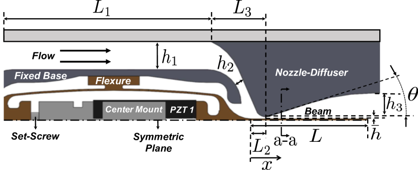
(a) Axial cross-section of flow geometry illustrating flow path.

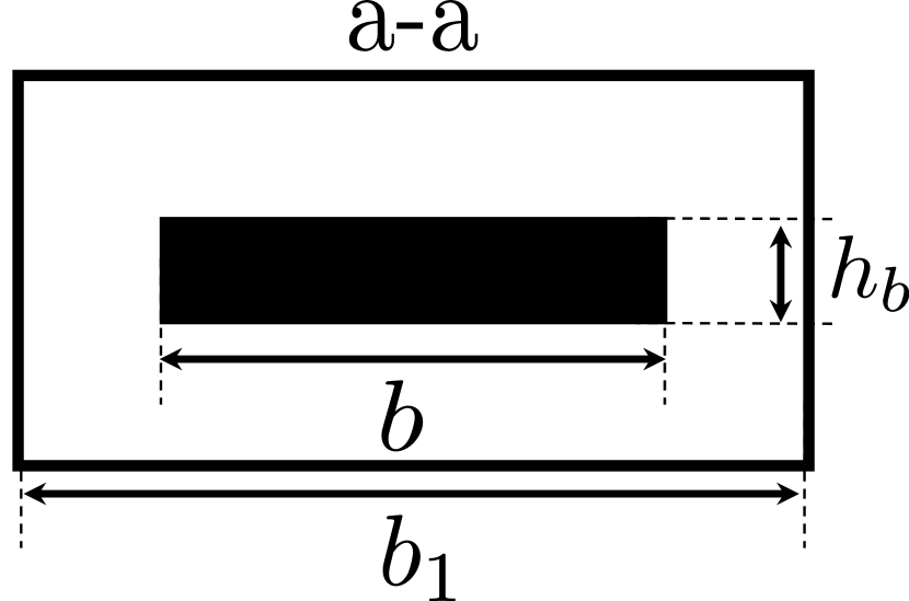
(b) Cut section a-a

Figure 1: Illustration of flow path and relevant geometry. Values and units are listed in table 5.

The flexure and the beam are made of a single aluminum stock, and comprise the moving structure. The fixed base is fastened with screws to both the test section and the flexure. The flexure behaves like a translational spring that transfers motion from the beam surface normal direction into compression and expansion of the piezoelectric stacks. The pre-stress from the set-screw and center mount ensure that the piezoelectric elements are always in compression: as the flexure moves above the channel centerline, the bottom stack is compressed, and the top stack pre-stress is released, although maintained positive, and vice-versa when the beam moves below the channel centerline. The up and down motion gives rise to two voltage signals that are $180^{\circ}$ out of phase. Vacuum grease and rubber inserts are used to seal and restrain the flow path to that shown in figure 1. An electrical fitting is used to connect the piezoelectric stacks to the data acquisition card on the outside of the test section.

The piezoelectric stacks are composed of multiple thin, alternately poled, piezoelectric layers “stacked”, or mechanically connected in series and electrically in parallel. They operate in what is known as the 33 mode, where the applied force is parallel to the poling direction. When a resistor is placed in parallel with the stack, its response to a step input force is that of an RC circuit with the capacitor having an initial voltage equivalent to the open circuit step-force voltage. The voltage $V(t)$ is measured across the resistor $R_{e}$ is given by $V(t)=V_{in}\exp\left(-t/R_{e}C^{*}_{p}\right).$ If the time constant $\tau=R_{e}C^{*}_{p}$ is large enough, the system will act as a low-pass filter and any oscillating voltage upstream of the resistor (opposite to ground) at a frequency $f_{res}$ that satisfies,

$$\omega_{\mathrm{res}}\gg\frac{1}{\tau}=\omega_{c},$$ (1)

will not pass through the resistor. Hence, the voltage output will be measured as if the system was an open circuit. We implement this circuit and choose an $R_{e}$ large enough such that the resonances of the structure satisfy condition 1. Specifically, we expect the stacks to act as strain gauges for high enough frequencies, where the output oscillating voltage is proportional to the flextensional displacement.

The combination of the flow path, the structure, the piezoelectric elements, and the electronics comprise the flow-energy harvester design. In our current work, we are particularly interested in the coupling between the flextensional and beam structure to the flow path in the channel.

2.2 Flextensional and beam parameters

Figure 2 divides the flow-energy harvester into two distinct parts: the flextensional dynamics on the left, which provides the boundary condition for the flow-driven beam dynamics on the right.

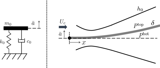
Figure 2: Illustration cantilever beam in a converging-diverging channel geometry (right) with simple harmonic boundary condition (left).

Table 1: Table of fluid-structure dimensional parameters.

Variable	Description	Dimension
$\delta$	beam displacement	$l$
$x$	beam length coordinate	$l$
$t$	time	$t$
$p$	pressure	$m*l^{-1}*t^{-2}$
$U_{c}$	characteristic velocity	$l*t^{-1}$
$k_{0}$	flexure stiffness	$m*t^{-2}$
$c_{0}$	flexure damping	$m*t^{-1}$
$m_{0}$	flexure mass	$m$
$L$	beam length	$l$
$h_{b}$	beam thickness	$l$
$b$	beam width	$l$
$\bar{h}$	throat height	$l$
$\rho_{f}$	fluid density	$m*l^{3}$
$\mu_{f}$	fluid viscosity	$m*l^{-1}*t^{-1}$
$\rho_{s}$	beam density	$m*l^{-3}$
$E$	Young’s modulus	$m*l^{-1}*t^{-2}$

Informed by finite element results of the flexture (Tosi, 2019), a damped harmonic oscillator can be used to capture the flextensional fundamental mode dynamics. In particular,

$$\frac{m_{0}}{b}\ddot{\bar{a}}+\frac{c_{0}}{b}\dot{\bar{a}}+\frac{k_{0}}{b}\bar{a}=f_{r},$$ (2)

where $\frac{m_{0}}{b}$, $\frac{c_{0}}{b}$, and $\frac{k_{0}}{b}$ are the flexure mass, damping, and stiffness constants per unit span, and $\bar{a}$ is the displacement of the flextensional boundary. The force $f_{r}$ is equivalent to the total force per unit span acting on the flexure interface to the cantilever. It can be defined as the integrated pressure difference between top and bottom channels over the beam length,

$$f_{r}=\int_{0}^{L}\Delta Pdx.$$ (3)

Here $\Delta P=P^{\mathrm{bot}}-P^{\mathrm{top}}$, and $P^{\mathrm{bot}}(x,t)$ and $P^{\mathrm{top}}(x,t)$ are the pressures acting on the bottom and top of the beam, per superscript. Values for $m_{0}$, $c_{0}$ and $k_{0}$ are inferred from measurements of the actual device in section 3.1.

The goal of our work is to understand the flutter instability when the system is near zero displacement. Hence, to describe the beam motion in transverse vibration, we consider the undamped, Euler-Bernoulli beam equation per unit span (Inman, 2008),

$$\rho_{s}h_{b}\frac{\partial^{2}}{\partial t^{2}}\delta(x,t)+\frac{\partial^{2}}{\partial x^{2}}\left(\frac{EI}{b}\frac{\partial^{2}}{\partial x^{2}}\delta(x,t)\right)=\Delta P,$$ (4)

where the $I$ is the area moment of inertia in equation 79. The beam is moving at its leading edge and free at its trailing edge, so the boundary conditions are

$$\delta(0,t)=\bar{a},\ \frac{\partial}{\partial x}\delta(0,t)=0,\ \frac{\partial^{2}}{\partial x^{2}}\delta(L,t)=0,\ \frac{\partial^{3}}{\partial x^{3}}\delta(L,t)=0.$$ (5)

Equation 4 and data 5 assume that the beam is thin relative to its length ($L>>h_{b}$); that the rotational inertia is negligible; and that beam extension and shear displacement are negligible when compared with the transverse displacement (the beam is inextensible). It follows that flow shear stresses do not impact the motion of the elastic member. Furthermore, the amplitude of oscillation is small relative to the beam length ($\left|\left|\delta\right|\right|_{\infty}\ll L$) such that $x$ is equivalent to the Lagrangian coordinate of the beam. These simplifications are consistent with our system near the zero displacement equilibrium.

Though equation 4 is undamped, external damping due to the fluid (i.e. Rayleigh damping) is accounted for within the pressure terms on its right-hand-side. Internal damping (i.e. internal to the solid), however, is not accounted within our equations of motion. A range of internal material damping formulations exist for a beam (Banks & Inman, 1991). Typically a strain-rate proportional form (Kelvin-Voigt) is used but time- or spatial- hysteretic formulations have also been deemed appropriate for certain materials and configurations. Yet material coefficients corresponding to any of the aforementioned formulations are difficult to obtain and require specialized experimental equipment. The effect of neglecting internal material damping results in underestimating the energy dissipated by the beam structure, leaving modes associated with the flexible beam specially susceptible to instabilities. However, the experimental results in section 3.2.1 show that the flextensional rigid-body motion at the cantilever base is responsible for the flutter bifurcation observed, rendering the flutter stability boundary observed largely independent of the beam modes. However, this limitation of the present model should be noted if it is generalized to designs that rely on significant beam bending. Results are verified and discussed in more detail within the numerical simulation and modeling in sections 4.2 and 5.5, respectively.

In considering the flow separately in the top and bottom channels, we write the geometrical constraint,

$$\delta(x,t)=\delta^{\mathrm{top}}(x,t)=-\delta^{\mathrm{bot}}(x,t).$$ (6)

Furthermore, we define $\delta=L\delta^{*}$, $t=\left(L/U_{c}\right)t^{*}$, $f_{r}=\rho_{f}U_{c}^{2}Lf_{r}^{*}$, and $\Delta P=\rho_{f}U_{c}^{2}\Delta P^{*}$ where $*$ superscript represents non-dimensional quantities. The non-dimensionalization of equations 2 and 4 as such yields the fluid-structure non-dimensional groups in table 2. A gap-to-length ratio, $\hat{h}=\bar{h}/L$ arises in dimensional analysis when we define a second length-scale $\bar{h}$ associated with the channel geometry $h_{0}=\bar{h}h_{0}^{*}$, as does the beam width-to-length ratio, $\hat{b}=b/L$. The relevant fluid-only dimensional groups depend on the form of the pressure term, as related to the velocity field.

This model is intended to describe the initial, small displacement behavior of the fluid-structure system as a function of fluid/structure parameters, and is appropriate for the stability analyses that follow in section 5.

Table 2: Table fluid-structure non-dimensional parameters for flextensional boundary and cantilevered beam.

Variable	Expression	Description
$\hat{m}_{\mathrm{bc}}$	$\frac{1}{\rho_{f}L^{2}}\frac{m_{0}}{b}$	boundary mass ratio
$\hat{k}_{\mathrm{bc}}$	$\frac{1}{\rho_{f}U_{c}}\frac{k_{0}}{b}$	boundary stiffness ratio
$\hat{c}_{\mathrm{bc}}$	$\frac{1}{\rho_{f}U_{c}L}\frac{c_{0}}{b}$	boundary damping ratio
$\hat{m}$	$\frac{\rho_{s}h_{b}}{\rho_{f}L}$	beam mass ratio
$\hat{k}$	$\frac{E}{\rho_{f}U_{c}^{2}}\frac{I}{bL^{3}}$	beam stiffness ratio

3 Experiments

From the design and parameter definitions in the previous section, we first experimentally measure the flextensional boundary parameters values in section 3.1, then quantify the dynamics of the device as a function of flow rate in section 3.2. Rather than a complete experimental characterization of the dynamics however, three settings are selected (and measured) instead, i.e. a baseline, high, and low set-screw torque values (shown in table 3), to span a range of flextensional mass, stiffness, and damping properties for comparison with the numerical simulation and modeling results in sections 4 and 5, respectively.

3.1 Flexure characterization

Two experiments are carried out to quantify $m_{0}$, $c_{0}$, and $k_{0}$, all in still air at standard pressure and temperature (STP). First, the flexure stiffness $k_{0}$ is characterized through a static measurement of force $F_{a}$ for displacement $\bar{a}$,

$$k_{0}=\frac{bf_{r}}{\bar{a}}=\frac{F_{a}}{\bar{a}},$$ (7)

derived from the steady equation 2. The second experiment measures the voltage output of the PZT stacks when the flextensional fundamental mode is excited. This is done with an impulse force at the $x=0$ location (figure 1). With the damped resonant frequency $\omega$ and exponential decay rate $\zeta$ measured from PZT voltage outputs, the solution to the homogeneous equation 2 ($f_{r}=0$) is used to map the dynamic voltage response to parameter properties as,

$$m_{0}=\frac{k_{0}}{\omega^{2}+\zeta^{2}},$$ (8)

$$c_{0}=2\zeta m_{0}.$$ (9)

Equations 7, 8, and 9 allow us to map experimentally measured quantities $F_{a}$, $\zeta$, and $\omega$ onto $k_{0}$, $c_{0}$, and $m_{0}$.

Table 3: Table of calculated mean flextensional properties.

Variable	Flex. 1	Flex. 2	Flex. 3
$\tau_{S}$ [Nm]	1.2	2	0.8
$k_{0}$ [N/m]	3.73E4	4.12E4	2.16E4
$m_{0}$ [kg]	0.0274	0.0204	0.0366
$c_{0}$ [kg/s]	0.135	0.314	0.281

3.2 Flow experiments

Next, the flextensional energy harvester is tested in flowing conditions to quantify the critical properties at the flutter instability, which encompass those properties at or near the quasi-stable point where the systems transitions from the stable equilibrium into flutter and vice-versa. Parameters are systematically varied in two ways: first, the set-screw torque $\tau_{S}$ sets the structural parameters of the flextensional corresponding to the boundary conditions in figure 2 and to values in table 3. Second, for any of the three set-screw settings (i.e flex. 1, 2, and 3), an experiment is run where the flow rate is first increased past the critical point, where the stable equilibrium to flutter transition is observed; then decreased past the fold point where the flutter transition to a stable equilibrium is observed. This topology holds true for all three settings tested. The dynamics of the flowing system are assessed by measuring the voltage output from each piezoelectric stack, and by processing video images of the beam displacement. In the increasing flow rate branch, the critical point is described by the critical flow rate $Q_{\mathrm{cr}}$ where the system is not longer stable, and the critical frequency $f_{\mathrm{cr}}$, corresponding to the dominant oscillatory frequency at the nearest point $Q\geq Q_{\mathrm{cr}}$ where self-sustained oscillations can be observed in the measured outputs. The fold point in the decreasing flow rate branch is characterized by the fold flow rate $Q_{\mathrm{r}}$. This data provides quantitative values by which we can compare numerical and analytical results in the subsequent sections.

Two output data products are extracted from experiments: PZT voltages and beam displacement videos. The voltage data set is processed through peak extraction to obtain average amplitudes over the relevant time series, and fast Fourier transformed using Welch’s method to obtain the signal frequency response corresponding to the highest peak. No other processing technique or filtering was applied to the voltage signals, as the system is responding to oscillatory forcing that satisfies condition 1. The video data set is decomposed and processed to characterize predominant vibration modes and their amplitudes. From the video, the transverse displacement of a section of the elastic beam is measured using edge-detection through a Canny filter (Canny, 1986) for the top and the bottom edges of the beam. The precision per-pixel is $\approx 0.15$ mm or $\approx 0.4$ % of the beam length. The extracted edges are averaged to estimate the beam center-line displacement. The resulting space-time series is processed using the spectral proper orthogonal decomposition (SPOD), which allows the most energetic mode shapes at each frequency to be robustly extracted (Schmidt et al., 2017; Towne et al., 2018). Further details of the SPOD applied here are given in appendix C. In subsequent results, frequencies are labelled as $f$ with subscript 1 representing that of the highest power spectral density (PSD) value, and subsequent peaks following numerically.

3.2.1 Experimental Results

The video and voltage data sets are processed for the three flextensional settings over air flow rates ranging from 5 to 500 L/min. The dynamics observed as the flow rate increases are consistent for all three flextensional settings: small decaying beam displacement and voltage amplitude behavior prevails until a critical flow rate is reached. At the critical flow rate, both the beam and PZT voltage amplitudes significantly increase and display self-sustaining oscillations (i.e. limit-cycle).

Figure 3 shows a representative example for flextensional setting 1 when the system has reached the self-sustained oscillation regime. The data set is at flow rate $Q=246$ L/min, 38 L/min above the flextensional setting 1 critical flow rate of 208 L/min. The spectrum shows a clear peak at $f_{1}=197$ Hz, and the corresponding mode contains more than 99% of the variance in the PSD of the beam displacement. The phase diagram shows a limit-cycle behavior and the mode shape resembles the rigid body motion of the cantilever base, denoting excitation of the flexure itself. Given the predicted cantilever fundamental mode frequency of 346 Hz from classical Euler-Bernoulli beam theory for clamped-free cantilever boundary conditions (shown in appendix D), we can reasonably associate the second peak at $f_{2}=341$ Hz to the beam fundamental mode. This is further validated from the mode shape shown: though the extracted transverse displacement data does not reach the cantilever base, the mode shape monotonically decreases as $x/L$ decreases without the appearance of a fixed node. The illustrated mode shape also contains over 99% of the variance of the signal at $f_{2}$. The phase diagram shows behavior typical of a lightly-damped resonance, where the mode amplitude and velocity are perturbed around their equilibrium points through sporadic forcing (Schmidt et al., 2018). The remaining peaks shown in the power spectrum plot are harmonics of $f_{1}$. Similar behavior was observed for flextensional settings 2 and 3 results, where $f_{2}\approx 341$ Hz appears in all three settings.

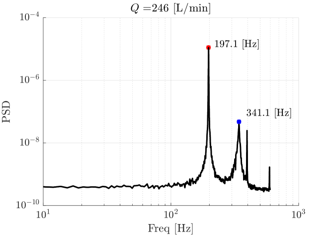
(a) Trace of cross-spectral density matrices at discrete frequencies.

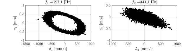
(b) Phase diagrams for mode 1 (left) and mode 2 (right).

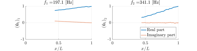
(c) SPOD mode shapes for mode 1 (left) and mode 2 (right).

Figure 3: Representative SPOD data for flextensional setting 1 showing self-sustained oscillating regime of mode 1 and under-damped regime of mode 2.

Figures 4 and 5 display the dominant mode (mode 1) amplitude and frequency, respectively, as a function of flow rate for all three flextensional settings. The amplitudes are obtained by projecting the beam transverse position space-time series onto the two most energetic spatial SPOD modes of $f_{1}$ and $f_{2}$, per the method described in the appendix. The mean and standard deviation (markers and error bars, respectively) of the resulting modal amplitude time-series corresponding to the highest PSD frequency are plotted in figure 4. To look for hysteresis, tests are carried out by first increasing then decreasing the flow rate. Plots in figure 4 show that the primary mode amplitude remains small (lightly-damped resonance) until a critical flow rate $Q_{\mathrm{cr}}$ is reached, which demarcates a transition to a high-amplitude, limit-cycle regime. Increasing the flow rate beyond $Q_{\mathrm{cr}}$, however, does not significantly increase the resulting amplitude. A slight amplitude decrease is sometimes seen at the highest flow rates, corresponding to the point when the beam appears to collide with the throat. As the flow rate is decreased through $Q_{\mathrm{cr}}$, a hysteresis loop becomes evident in all three flextensional settings, with its size ($\Delta Q=Q_{\mathrm{cr}}-Q_{\mathrm{r}}$) varying between each setting. The system recovers the small amplitude regime at $Q<Q_{\mathrm{r}}<Q_{\mathrm{cr}}$, where $Q_{\mathrm{r}}$ is the fold flow rate. This hysteresis suggests that the system is undergoing a subcritical Hopf bifurcation at $Q_{\mathrm{cr}}$, giving rise to the bi-stable region captured in the data. All three frequency responses in figure 5 appear constant until $Q_{\mathrm{cr}}$ is reached, at which point the frequencies tend to increase slightly with increasing flow rate. The hysteretic behavior is most pronounced in the frequency data from setting 2. Critical and fold properties for the observed bifurcation are summarized in table 10.

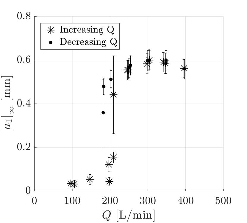
(a) Flextensional 1.

(b) Flextensional 2.

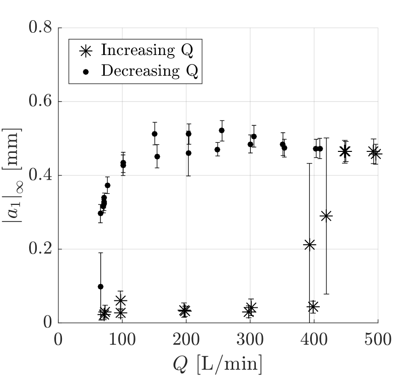
(c) Flextensional 3.

Figure 4: Video data set showing mode 1 amplitude vs. flow rate for all flextensional settings.

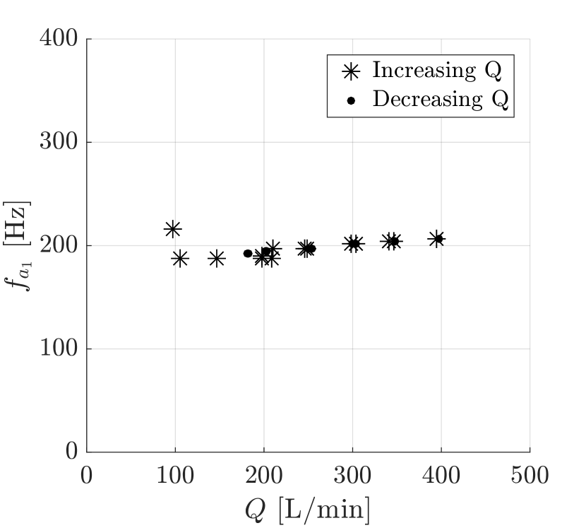
(a) Flextensional 1.

(b) Flextensional 2.

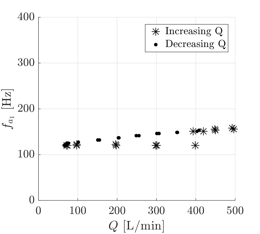
(c) Flextensional 3.

Figure 5: Video data set showing mode 1 frequency response vs. flow rate for all flextensional settings.

Analogous amplitude and frequency plots for the PZT voltage are shown in figures 6 and 7, respectively, with critical and hysteresis results in agreement with video displacement data. One discrepancy however, is observed in the flex. 3 frequency data. Specifically, the plot shows the beam fundamental frequency as dominant until $Q_{\mathrm{cr}}$, at which point the voltage response frequency is double that of the video displacement frequency in figure 5. This effect is caused by lightly pre-stressed piezoelectric elements, as this flexure configuration represents conditions with the least amount of torque applied on the set-screw. The phenomenology is as follows: once the oscillation reaches the full extension at either the top or bottom of the flextensional stroke, the decompressed stack looses contact with the flexure structure. This in turn causes a strong response that flips the sign of the voltage output, and appears as a frequency doubling through the discrete Fourier transform. The nonlinear loss-of-contact behavior has been observed by (Sherrit et al., 2009) as flextensional actuators loose their bond between stacks and the flexure. Voltage amplitudes are also notably lower in flexure setting 3 than the other two flexure configurations.

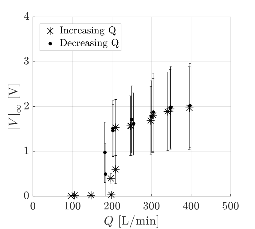
(a) Flextensional 1.

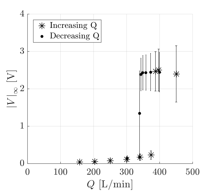
(b) Flextensional 2.

(c) Flextensional 3.

Figure 6: PZT 1 voltage amplitude vs. flow rate for all flextensional settings.

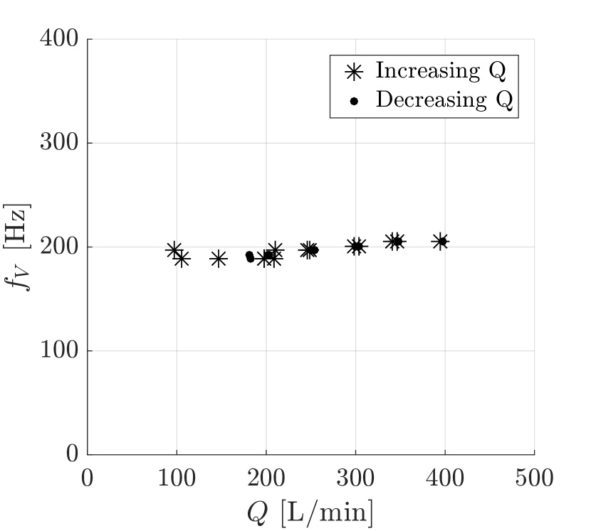
(a) Flextensional 1.

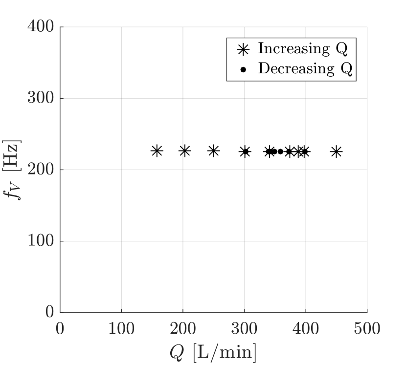
(b) Flextensional 2.

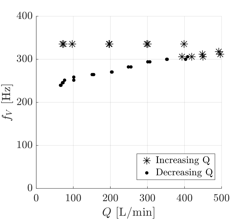
(c) Flextensional 3.

Figure 7: PZT 1 frequency primary peak is voltage power spectral density vs. flow rate for all flextensional settings.

Table 4: Table of critical and restoring (fold) values for flextensional settings.

Variables	Flex. 1	Flex. 2	Flex. 3	Description
$Q_{\mathrm{cr}}$ [L/min]	208	376	410	critical flow rate
$Q_{\mathrm{r}}$ [L/min]	179	334	73	fold flow rate
$f_{\mathrm{cr}}$ [Hz]	186	226	120	critical frequency

Given the observed $Q_{\mathrm{cr}}$ values in table 10, it is plausible that throat velocities may reach a considerable fraction of the sound speed when operating in air. In appendix B, we estimate the Mach number at the channel throat $\mathcal{M}_{\mathrm{t}}$. We discuss the potential limitations of the incompressible flow assumption made in the subsequent simulation section next.

4 Numerical Simulations

Experimental results from the previous section show a rich set of dynamics and different regimes consistent with a subcritical Hopf bifurcation. In this section, we use two-way coupled numerical simulations of a beam in the converging-diverging channel in order to investigate the three-dimensional flow field and provide insights into the flow patterns and instability mechanisms that drive the bifurcation. Experimental results also point us primarily to explore the flextensional mode dynamics, the only one that reaches the limit-cycle, for which the beam is essentially in rigid-body motion. We thus consider a rigid beam that is allowed to oscillate, via the lumped parameter model, using the experimentally-measured values for mass, stiffness, and damping ratios for flextensional setting 1. We further discuss the validity of the rigid-body approximation below and well as in section 5.

4.1 Numerical method

Our simulations are based on the lattice Boltzmann method (LBM), which originates from kinetic theory and thus evolves discretized particle distribution functions (populations) $f_{i}(\bm{x},t)$, which are associated with discrete velocities $\bm{c}_{i},i=1,\ldots,Q$ and designed to recover the macroscopic Navier-Stokes equations (NSE) in the hydrodynamic limit. By organizing the set of discrete velocities into a regular lattice, LBM eventually reduces to a simple, efficient, and scalable stream-and-collide algorithm with the additional advantage of exact propagation and local non-linearity, which is incorporated through the collision operator. In recent years, LBM has made significant progress and early stability issues of the classical lattice Bhatnagar–Gross–Krook (LBGK) model have been overcome. While on one hand explicit turbulence models have shown success for turbulent flows (Chen et al., 2003; Malaspinas & Sagaut, 2012), the class of parameter-free entropic lattice Boltzmann schemes (ELBM) have shown accurate and robust solutions for both resolved and under-resolved simulations for laminar, transitional as well fully turbulent flows (Bösch et al., 2015a, b; Dorschner et al., 2016, 2017b). In particular, we use the multi-relaxation time (MRT) variant of ELBM (KBC) (Karlin et al., 2014), which exploits the high dimensionality of the kinetic system and chooses the relaxation of higher-order, non-hydrodynamic moments such that the entropy of the post-collision state is maximized. The KBC model has been discussed in various contributions and we will restrict ourselves to the main steps in case of isothermal flow using the standard $D3Q27$ lattice.

We start from the general lattice Boltzmann equation for the population $f_{i}(\bm{x},t)$:

$$f_{i}(\bm{x+c_{i}},t+1)=f_{i}^{\prime}=(1-\beta)f_{i}(\bm{x},t)+\beta f_{i}^{\text{mirr}}(\bm{x},t),$$ (10)

where the streaming step is indicated by the left-hand side and the post-collision state $f^{\prime}_{i}$ on the right-hand side is given by a convex-linear combination of $f_{i}(\bm{x},t)$ and a mirror state $f_{i}^{\text{mirr}}(\bm{x},t)$. We use natural moments to represent the population as a sum of the kinetic part $k_{i}$, the shear part $s_{i}$ and the remaining higher-order moments $h_{i}$:

$$f_{i}=k_{i}+s_{i}+h_{i}.$$ (11)

The mirror state can thus be represented as

$$f_{i}^{\text{mirr}}=k_{i}+\left(2s_{i}^{\rm eq}-s_{i}\right)+\left(\left(1-\gamma\right)h_{i}+\gamma h_{i}^{eq}\right),$$ (12)

where $s_{i}^{eq}$ and $h_{i}^{eq}$ denote $s_{i}$ and $h_{i}$ evaluated at equilibrium.

The equilibrium distribution function $f^{\rm eq}$ is defined as the minimum of the entropy function

$$H(f)=\sum_{i=1}^{Q}f_{i}\ln\left(\frac{f_{i}}{W_{i}}\right),\\$$ (13)

subject to the local conservation laws for mass and momentum

$$\sum_{i=1}^{Q}\{1,\bm{c_{i}}\}f_{i}=\{\rho,\rho\bm{u}\},$$ (14)

and the weights $W_{i}$ are lattice-specific constants. By minimizing the $H$-function in the post-collision state one obtains the relaxation parameter

$$\gamma=\frac{1}{\beta}-\left(2-\frac{1}{\beta}\right)\frac{\left<\Delta s|\Delta h\right>}{\left<\Delta h|\Delta h\right>},$$ (15)

where $\Delta s_{i}=s_{i}-s_{i}^{\text{eq}}$ and $\Delta h_{i}=h_{i}-h_{i}^{\text{eq}}$ are the deviation from equilibrium and the entropic scalar product is defined as $\left<X|Y\right>=\sum_{i}(X_{i}Y_{i}/f_{i}^{\text{eq}})$. The KBC model recovers the Navier-Stokes equations in the hydrodynamic limit for which the viscosity is related to the parameter $\beta$ as

$$\nu=c_{s}^{2}\left(\frac{1}{2\beta}-\frac{1}{2}\right),$$ (16)

where $c_{s}=1/\sqrt{3}$ is the lattice speed of sound.

Finally, to include two-way coupling of the fluid with the cantilever beam, we follow the procedure as outlined in (Dorschner et al., 2015, 2017a, 2018), using second-order Grad boundary conditions to account for the momentum transfer from the fluid onto the beam and vice versa. The beam velocity, needed to prescribe the boundary conditions, is obtained by solving Newton’s equations of motions using an Euler integration and the fluid force is evaluated by the Galilean invariant momentum exchange method (see Wen et al. (2015)). This procedure has been validated extensively for various test-cases for one- and two-way coupled simulations as well as fully coupled fluid-structure interaction problems involving deforming geometries.

4.2 Simulation of the flow energy harvester

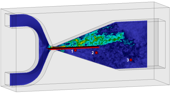
Figure 8: Instantaneous snapshot of the computational setup for $Q=208$ L/min, showing a slice of velocity magnitude. Exemplary observer points are indicated by the red spheres.

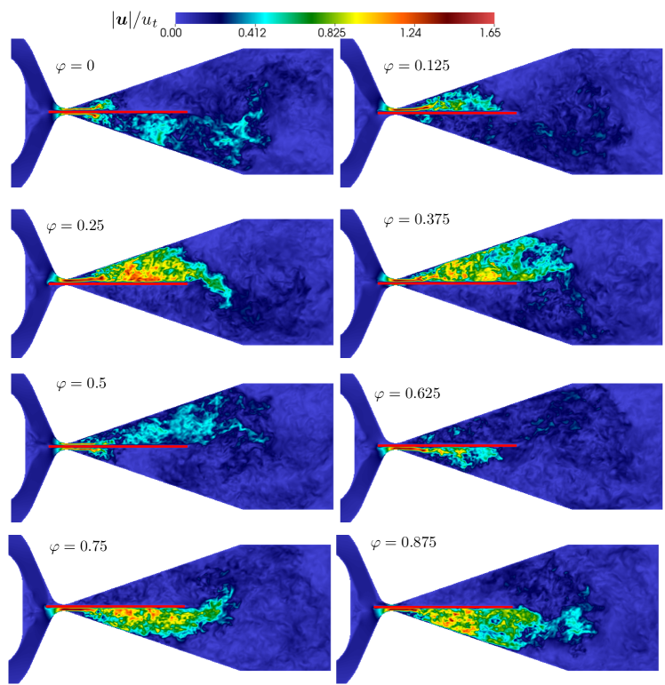
Figure 9: Flow evolution for one period of the energy harvester, showing a slice of velocity magnitude.

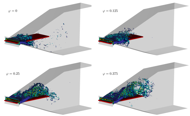
Figure 10: Flow evolution for half a period of the energy harvester, showing isosurfaces of vorticity colored by velocity magnitude and zoomed into the diffuser region.

The simulation of the full flextensional energy harvester is a challenging task due to the complex interaction of various physical mechanisms. We keep the geometry of the fluid channel path identical to the experimental setup apart from the diffuser exit, which is a sharp edge in the simulation but smoothed in the experiment. In figure 8, the numerical setup is shown. As noted in section 2.2, the flexure itself is modeled by a harmonic oscillator to which a rigid cantilever beam is attached. In the simulations, this is realized by elastically translating boundary conditions of the beam. The mass, stiffness and damping ratio of the harmonic oscillator are prescribed in the simulations according to the experimental measurements of flex. setting 1 in table 3.

Regarding the rigid-body approximation, as discussed in sections 2 and 3, we refrain from modeling the beam bending since the most energetic observed mode is primarily a rigid body motion of the entire flexure, and where the damping of the structure as a whole is well approximated by a second-order damped harmonic oscillator. We preformed precursor simulations that included elasticity of the beam but neglecting internal damping, and these confirmed the model predictions discussed in section 5, namely that higher-order oscillatory beam modes do become unstable in the absence of internal damping. Based on the experiments, these results are known to be unphysical and we therefore focus our attention to predicting critical properties of the first, primarily rigid, flextensional based mode. As discussed in appendix B, we do not account for compressibility and treat the fluid as incompressible fluid. Our simulations are carried out on a uniform Cartesian mesh (with $\Delta=1$ and $\Delta t=1$ in lattice units), where we resolve the beam with roughly $250$ lattice points. All other dimensions follow from the experimental setup and a snapshot of the computational domain is shown in figure 8. Further, the inflow velocity is conservatively set to $u=0.0075$ (in lattice units) to avoid any compressibility effects. The Reynolds number is set to $Re_{h}=u_{t}\bar{h}/\nu\approx 5200$, which is chosen such that it is high enough to account for viscous effects but low enough to provide sufficient resolution for all pertinent flow scales. To that end, convergence of the critical flow rates was verified with coarser meshes. In addition, the agreement with experiments gives us confidence that all pertinent mechanisms are captured by our simulations.

Figure 9 shows the evolution of the velocity magnitude in the mid-plane of the domain for one representative cycle. In the beginning of each cycle for a phase angle $\varphi=0$ the beam displacement is zero and two symmetric jets on the top and bottom of the beam are forming. Note also that residual turbulence from the previous cycle is visible in the bottom half of the diffuser. Subsequently for $\varphi=0.125$, the beam moves downward, leading to an increase of mass flow through the upper diffuser channel until the mass flow through the bottom channel almost ceases at $\varphi=0.25$. Consequently, the upper jet amplifies and penetrates deeper into the diffuser until it eventually breaks up into turbulence beyond the beam. The maximum penetration of the jet into the diffuser is reached at $\varphi=0.25$. Notably, the jet does not penetrate much beyond the length of the beam, where it is then expanding into the bottom half of the domain and rapidly broken up into finer-scale turbulence. During its upward motion beyond $\varphi=0.25$, the upper jet weakens whereas the mass flow rate through the bottom half of the domain gradually increases. Finally at $\varphi=0.5$, the process repeats in a symmetric fashion for the bottom half of the channel. In figure 10, vorticity isosurfaces colored by velocity magnitude are shown for the first half of the oscillation period. The behavior is analogous to what was observed for the velocity magnitude. However, we can additionally observe the effect of spanwise confinement. Starting from a phase angle of $\varphi=0.25$, one can observe vortical structures attaching to the side and upper walls of the diffuser geometry. Downstream of the throat, a large lambda-type vortex structure is formed on the upper diffuser wall due to vortex rollup from both sides of the beam. Consequently, most vorticity is confined in the center region of the beam, whereas only negligible vorticity is found in regions close to the diffuser side walls and downstream of the throat.

To assess the predictive capabilities and validity of our computational model, we run a series of simulations for flow rates in the range of $Q=100$ to 300 L/min and record the time evolution of the beam displacement. This allows us to obtain an estimate of the critical flow rate at which the beam starts to exhibit self-sustained oscillations. As shown in figure 11, the critical flow rates as computed by our simulations agree well with the experiments.

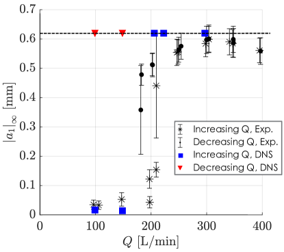
Figure 11: Beam oscillation amplitude as a function of the flow rate for the experiments as well as the numerical simulations.

Note that in the simulation it is not possible to fully resolve the thin fluid layer between beam and the throat for the experimental geometry. This is due to the fact that in our experiments, and as indicated in figure 4, the beam oscillation amplitude becomes large and sometimes collides with the wall (see error bars). Such collisions are not explicitly modeled in our numerical model. However, since we are only interested in the on-set of self-sustained oscillation we stop the simulation once the beam displacement reaches the height of the throat. In addition to recording the oscillation amplitude for various flow rates, we also probe the hysteresis behavior of the system to access the bifurcation type. To that end, the simulation of $Q=208$ L/min is restarted and the flow rate reduced. As shown in figure 11, we observe a pronounced hysteresis behavior, again indicative of a subcritical Hopf bifurcation, and is in agreement with the experimental findings. The hysteresis is, however, more pronounced in the simulations. One potential explanation comes from the perturbation and noise inherent in our experiments (i.e. collision of beam with channel wall), which would tend to push the beam states from the stable limit-cycle basin of attraction to that of the stable equilibrium earlier (i.e. at a higher flow rate than the fold point), resulting in a smaller experimental hysteresis loop. In figure 12(a), the evolution of the beam displacement as well as the power spectral density is shown for the critical flow rate of $Q=208$ L/min. As expected, the beam displacement undergoes exponential growth and, from the power spectral density, oscillates near the natural frequency of the flexure. Once again, this is consistent with what is observed in the experiment.

In addition to the temporal evolution of the beam displacement, three observer probes were placed within the domain. In particular, the probes were placed in vicinity of the throat, near the trailing edge of the beam as well as in the far field of the diffuser (see figure 8). The evolution of the streamwise velocity for all three probes is depicted in figure 13. Probe 1, located near the throat, shows periodic behavior with a largely constant amplitude and only a slight decrease in amplitude as the oscillation amplitude of the beam increases due to an increase of the throat gap. A different picture is drawn for the two probes downstream. It is apparent that the amplitude in the initial phase ($t/T_{b}<17$) remains relatively low and increases noticeably afterwards. This is due to the increasing penetration depth of the jet, which eventually reaches the probe location. In addition, the magnitude of the streamwise velocity rapidly decreases as it is diffused further downstream and diminishes to roughly $20\%$ for probe $2$. It is further is instructive to look at the power spectral density plots of the observer probes. It is noticeable that the most dominant frequency for probe 1 is the beam frequency, whereas further downstream its first harmonic becomes increasingly larger and eventually dominates. This can be explained by the fact that further downstream there is the coupling between jets in the lower as well as in the upper half of the domain, i.e., the probes feel the influence of both jets and thus doubling the dominant frequency.

Moreover, we measure the phase-averaged profile at $\varphi=0$ of the spanwise velocity in a cross section near the throat as shown in figure 15. The profile is symmetric and linear to a good approximation for most of the span. One can also see the effect of spanwise vortices, which are forming due to spanwise confinement at the edge of the beam. This will be used later as an input and validation of the model assumptions in section 5.

Finally, having an indication of how the flow evolves within the internal flow energy harvester helps support our conjecture that the main driving factor of the instabilities arising in the flow originates from its modulation due to the confinement in the channel throat. This is evidenced by the flow field in figure 9 and figure 10 where there are no significant flow structures that appear able to drive the instabilities in the wake of the beam. Further validation is presented next, where we devise a reduced-order model that accounts for this modulation phenomenon as the only source of the instability.

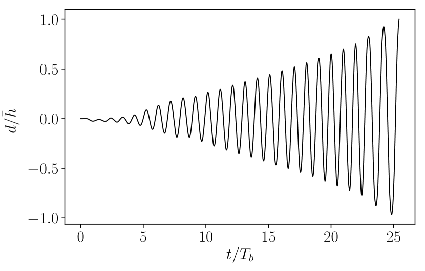
(a)

(b)

Figure 12: Evolution of the beam displacement and its power spectral density.

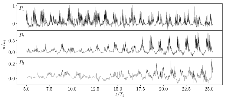
Figure 13: Evolution of the streamwise velocity profile for three probes.

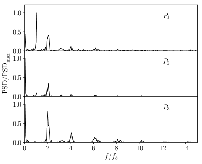
Figure 14: Spectral density of pressure for the observer points.

(a) Location of the phase-averaging plane.

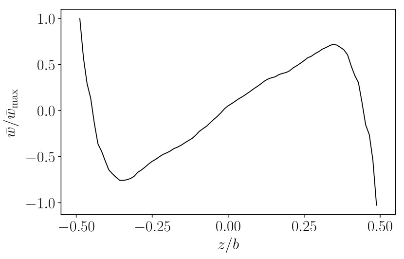
(b) Phase-averaged spanwise velocity profile.

Figure 15: Spanwise velocity profile.

5 Model

Armed with insights from our numerical simulations, we reduce the fluid-structure equations of motion to terms that are relevant when considering the flow modulation at the channel throat. In this section, we develop an incompressible fluid-structure model that captures the dynamics of the confined flow as the beam oscillates. In particular, we formulate the forces on the beam as a function of the channel area as modulated through the beam motion. The coupled equations of motion, once derived and linearized, represent the modulation of the flow rates through beam motion and confinement. The model presented is an extension of a viscous, quasi-one-dimensional model (Tosi & Colonius, 2019; Inada & Hayama, 1988, 1990; Nagakura & Kaneko, 1991; Fujita & Shintani, 1999, 2001, 2007), where here we include the effect of flow in the spanwise direction as an additional state solved through a spanwise momentum equation. The structure model is extended to include a moving beam boundary conditions to account for the motion of the flextensional transducer. The solid equations are defined in section 2.2 with the appropriate coupling to the fluid pressure. We begin by defining the pressure in terms of flow properties and channel geometry.

5.1 Fluid equations of motion

We consider a three-dimensional control volume analysis of the half-span section of the channel in order to obtain an expression that contains the $\mathbf{\hat{z}}$ momentum terms. We would like to obtain an expression of the local pressure to quantify the fluid force onto the flextensional structure. Figure 16 illustrates the control volume boundaries as a section of the diagram in figure 2, with only half of the channel demarcating the control surfaces in $\mathbf{\hat{z}}$. The surface normal vectors are

$$\left[\mathbf{n}_{1}\cdots\mathbf{n}_{6}\right]=\begin{bmatrix}1&-1&-\frac{dh_{0}}{dx}&\frac{d\delta}{dx}&0&0\\ 0&0&1&-1&0&0\\ 0&0&0&0&1&-1\\ \end{bmatrix}.$$ (17)

We assume the beam is rigid in $z$, such that $\delta=\delta(x,t)$. Solid walls are in $\mathbf{n}_{3}$ and $\mathbf{n}_{4}$, with $\mathbf{n}_{1}$, $\mathbf{n}_{2}$, $\mathbf{n}_{5}$, and $\mathbf{n}_{6}$ representing free surfaces.

(a) Projection view of channel control volume.

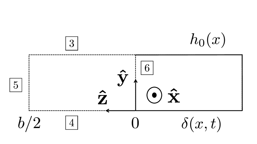
(b) Front view of channel control volume.

Figure 16: Three-dimensional control volume illustration for the spanwise quasi-1D leakage flow model.

We apply mass and momentum conservation to this control volume under the simplifying assumptions of constant fluid density and a gradually-varying channel in the streamwise direction, $h_{0}^{\prime 2}\ll 1$ and $\delta^{\prime 2}\ll 1$, such that $\sqrt{1+h_{0}^{\prime 2}}\approx 1$ and $\sqrt{1+\delta^{\prime 2}}\approx 1$ for $x\in[0,L]$. Starting with mass conservation and the three-dimensional velocity vector ${\bf u}=\left[u,v,w\right]^{T}$, we have

$$\frac{\partial}{\partial t}\left(\int_{0}^{b/2}\int_{\delta}^{h_{0}}dydz\right)+\frac{\partial}{\partial x}\left(\int_{0}^{b/2}\int_{\delta}^{h_{0}}udydz\right)+\left.\int_{\delta}^{h_{0}}wdy\right|_{z=b/2}=0.$$ (18)

Integrating in $z$ leads to

$$\frac{\partial Q_{x}}{\partial x}+\frac{2}{b}\left.Q_{z}\right|_{z=b/2}=\frac{\partial\delta}{\partial t},$$ (19)

where

$$Q_{x}=\int_{\delta}^{h_{0}}udy,\ Q_{z}=\int_{\delta}^{h_{0}}wdy,$$ (20)

are the flow rates per unit length in stream- and spanwise directions, respectively. In a similar manner, the momentum equations in $\mathbf{\hat{x}}$ can be obtained as,

$$\frac{\partial}{\partial t}\left(\int_{0}^{b/2}Q_{x}dz\right)+\int_{0}^{b/2}\frac{\partial\mathcal{N}_{x}}{\partial x}dz+\left.\mathcal{N}_{xz}\right|_{z=b/2}=$$ (21)

$$-\frac{1}{\rho_{f}}\left\{\int_{0}^{b/2}\left[\frac{\partial}{\partial x}\left(\int_{\delta}^{h_{0}}Pdy\right)-h_{0}^{\prime}P|_{y=h_{0}}+\frac{\partial\delta}{\partial x}P|_{y=\delta}\right]dz-F_{\mathrm{visc},x}\right\},$$

and in $\mathbf{\hat{z}}$,

$$\frac{\partial}{\partial t}\left(\int_{0}^{b/2}Q_{z}dz\right)+\frac{\partial}{\partial x}\left(\int_{0}^{b/2}\mathcal{N}_{xz}dz\right)+ \left.\mathcal{N}_{z}\right|_{z=b/2}=$$ (22)

$$\int_{\delta}^{h_{0}}\left(P|_{z=b/2}-P|_{z=0}\right)dy-F_{\mathrm{visc,z}},$$

where the advection terms are given by

$$\mathcal{N}_{x}=\int_{\delta}^{h_{0}}u^{2}dy,\ \mathcal{N}_{z}=\int_{\delta}^{h_{0}}w^{2}dy,\ \mathcal{N}_{xz}=\int_{\delta}^{h_{0}}uwdy.$$ (23)

The goal of this analysis is to obtain an expression for the pressure as a function of $\delta$, $Q_{x}$, and $Q_{z}$. To make further progress, we must find a closure for the advection terms $\mathcal{N}_{x}$, $\mathcal{N}_{z}$, and $\mathcal{N}_{xz}$, along with $F_{\mathrm{visc,x}}$ and $F_{\mathrm{visc,z}}$ in terms of those variables. Similarly, we must also relate the local pressure values in $y$ and $z$ to the integrated pressure over the same dimensions.

We consider the infinitessimal Navier-Stokes equations (NSE) in three dimensions non-dimensionalized similar to lubrication theory (Kundu et al., 2012),

$$\begin{gathered}x^{*}=\frac{x}{L},\ y^{*}=\frac{y}{\bar{h}},\ z^{*}=\frac{y}{b},\ u^{*}=\frac{u}{U_{c}},\ v^{*}=\frac{L}{\bar{h}U_{c}}v,\ w^{*}=\frac{w}{U_{c}}\varepsilon_{b},\ t^{*}=\frac{U_{c}}{L}t,\\ P^{*}=\frac{P}{P_{\mathrm{in}}},\ \hat{h}=\frac{\bar{h}}{L},\ \varepsilon_{b}=\frac{b}{L},\ Re_{L}=\frac{\rho_{f}U_{c}L}{\mu_{f}},\ \Lambda=\frac{\mu_{f}LU_{c}}{P_{\mathrm{in}}\bar{h}^{2}}.\end{gathered}$$ (24)

$P_{\mathrm{in}}$ is a constant reference pressure upstream of the channel as defined in equation 37. For $\hat{h}\rightarrow 0$, the NSE are well approximated by

$$0 =-\frac{1}{\Lambda}\frac{\partial P^{*}}{\partial x^{*}}+\frac{\partial^{2}u^{*}}{\partial y^{*2}}$$ (25)

$$0 =-\frac{1}{\Lambda}\frac{\partial P^{*}}{\partial y^{*}}$$

$$0 =-\frac{1}{\Lambda}\frac{\partial P^{*}}{\partial z^{*}}+\varepsilon_{b}^{2}\frac{\partial^{2}w^{*}}{\partial y^{*2}}.$$

To obtain a simple expression for the flow velocities, we first assume that the flow remains largely one-dimensional in $x$ for $u$ and $v$, and recover the quasi-1 dimensional parabolic profile of $u^{*}=u^{*}\left(y^{*}\left(x^{*}\right),t^{*}\right)$, with $v\approx 0$. Next we assume that any $\frac{\partial P^{*}}{\partial z^{*}}$ is due to the motion of the channel walls, and that no time-averaged net pressure gradient exists in $z$. It follows that, due to the symmetry of the geometry in figure 16, $\left.w^{*}\right|_{z=0}=0$ and $w^{*}$ odd in $z=\left[-\frac{b}{2},\frac{b}{2}\right]$ with $P^{*}$ symmetric in the same $z^{*}$ interval. If $\frac{\partial P^{*}}{\partial z^{*}}\neq 0$ and $P^{*}=P^{*}(x,z,t)$, the spanwise component in equation 25 can be integrated twice (with the no-slip conditions) to also recover a parabolic profile of $w^{*}$ in $y^{*}$. Combined with a linear function in $z^{*}$, the simplest that satisfies the specified symmetries, we assume a functional form for the spanwise velocity profile as

$$w^{*}(x^{*},y^{*},z^{*},t)\sim z^{*}\left(\frac{\delta(x^{*},t^{*})}{\bar{h}}-y^{*}\right)\left(\frac{h_{0}(x^{*})}{\bar{h}}-y^{*}\right).$$ (26)

As a first check to the conjecture that $w^{*}\sim z^{*}$, we consult the numerical simulation results and compute the phase-averaged $w$ at $\varphi=0$ near the throat as indicated in figure 15(a). Figure 15(b) shows that $w$ is linear to good approximation for most of the beam span. The deviation from the linear profile can be attributed to the channel spanwise confinement and the associated vortices forming at the corners of the beam edge. Even considering those effects, the linear approximation appears to be a reasonable trade-off between accuracy and simplicity. With an expression for $w^{*}$ as a function of $y^{*}$, $\mathcal{N}_{z}$ and $F_{\mathrm{visc,z}}$ can be defined in terms of $Q_{z}$,

$$\mathcal{N}_{z}=\xi_{z}\frac{Q_{z}^{2}}{h_{0}-\delta},\ F_{\mathrm{visc,z}}=-12\mu_{f}\frac{Q_{z}}{\left(h_{0}-\delta\right)^{2}},$$ (27)

with the latter taking the form for a Newtonian fluid. Here $\zeta_{z}=6/5$.

The remaining advection terms in equation 23 can be defined in terms of $Q_{x}$ and $Q_{z}$,

$$\mathcal{N}_{x}=\xi_{x}\frac{Q_{x}^{2}}{h_{0}-\delta},\ \mathcal{N}_{xz}=\xi_{xz}\frac{Q_{x}Q_{z}}{h_{0}-\delta},$$ (28)

where $\xi_{x}$ and $\xi_{xz}$ are constant profile “shape factor” for axial and axial-spanwise cross-coupling velocities. $F_{\mathrm{visc,x}}$ takes the form (Tosi & Colonius, 2019),

$$F_{\mathrm{visc,x}}=-\frac{f(Q_{x})}{4}\frac{Q_{x}^{2}}{\left(h_{0}-\delta\right)^{2}},$$ (29)

where the Fanning friction factor, $f$,

$$f=\begin{cases}48Re_{h}^{-1}&\text{if }Re_{h}<1000\\ 0.26Re_{h}^{-0.24}&\text{if }Re_{h}\geq 1000\end{cases},$$ (30)

with $Re_{h}=\hat{h}Re_{L}$. We model the profile shape factor as

$$\mathcal{\xi}_{x}=\mathcal{\xi}_{xz}=\begin{cases}6/5&\text{if }Re_{h}<1000\\ 1&\text{if }Re_{h}\geq 1000\end{cases},$$ (31)

where the laminar value ($Re_{h}<1000$) coincides with the lubrication theory frictional result (Kundu et al., 2012; Tosi & Colonius, 2019), and the turbulent case follows from the blunted mean velocity profile in the outer region and neglects the thin inner region.

Next, we define the relation between evaluated and integrated $P$ and $Q_{z}$ in $y$ and $z$. Substituting the form in equation 26 into the spanwise component of 25, we ascertain that $P^{*}\propto z^{*2}$. We keep integrated $z$ quantities as model variables, normalizing them such that they represent the spatial average of $P$ and $Q_{z}$ over $z=\left[0,\frac{b}{2}\right]$,

$$\bar{P}=\frac{2}{b}\int_{0}^{b/2}Pdz,\ \bar{Q}_{z}=\frac{2}{b}\int_{0}^{b/2}Q_{z}dz.$$ (32)

With the definition of $w$ from $w^{*}$ in equations 24 and 26, along with the definitions immediately above, we have,

$$\left.P\right|_{z=0}=\frac{3}{2}\bar{P},\ \left.Q_{z}\right|_{z=b/2}=2\bar{Q}_{z}.$$ (33)

Mass conservation in equation 19, and axial and spanwise momentum, equations 21 and 22, can now be simplified to,

$$\frac{\partial Q_{x}}{\partial x}+\frac{4}{b}\bar{Q}_{z}=\frac{\partial\delta}{\partial t}.$$ (34)

$$\frac{\partial Q_{x}}{\partial t}+\frac{\partial}{\partial x}\left(\xi_{x}\frac{Q_{x}^{2}}{h_{0}-\delta}\right)+4\xi_{xz}\frac{Q_{x}\bar{Q}_{z}}{b\left(h_{0}-\delta\right)}=-\frac{1}{\rho_{f}}\frac{\partial\bar{P}}{\partial x}\left(h_{0}-\delta\right)+F_{\mathrm{visc,x}}.$$ (35)

$$\frac{\partial\bar{Q}_{z}}{\partial t}+\frac{\partial}{\partial x}\left(\xi_{xz}\frac{Q_{x}\bar{Q}_{z}}{h_{0}-\delta}\right)+ 8\xi_{z}\frac{\bar{Q}_{z}^{2}}{b\left(h_{0}-\delta\right)}=$$ (36)

$$-\frac{2\left(h_{0}-\delta\right)}{b\rho_{f}}\left(P|_{z=b/2}-\frac{3}{2}\bar{P}\right)-\frac{12\mu_{f}}{\rho_{f}}\frac{\bar{Q}_{z}}{\left(h_{0}-\delta\right)^{2}}$$

Equations 34, 35, and 36 comprise the fluid equations of motion that describe the averaged spanwise local pressure in $x$ as a function of the passage shape and dynamics. Pressure boundary conditions are required to solve them uniquely. Based on leakage-flow instability work (Nagakura & Kaneko, 1991; Inada & Hayama, 1988, 1990; Tosi & Colonius, 2019),

$$\bar{P}(t)|_{x=0} =P_{\mathrm{in}}-\frac{\zeta_{\mathrm{in}}}{2}\rho_{f}\left[\left(\frac{Q_{x}}{h_{0}-\delta}\right)^{2}\right]_{x=0},$$ (37)

$$\bar{P}(t)|_{x=L} =P_{\mathrm{out}}+\frac{\zeta_{\mathrm{out}}}{2}\rho_{f}\left[\left(\frac{Q_{x}}{h_{0}-\delta}\right)^{2}\right]_{x=L}.$$

where $\zeta_{\mathrm{in}}\geq 1$ and $\zeta_{\mathrm{out}}\geq 0$ are loss coefficients, and the departure from equality represents non-isentropic processes. $P_{\mathrm{in}}$ and $P_{\mathrm{out}}$ are constants. The boundary value for $P|_{z=b/2}$ appears explicitly in equation 36, and is an additional boundary condition needed for the control volume in figure 16. We maintain the same form to define the pressure at the edge surface $z=b/2$,

$$P(x,t)|_{z=b/2}=p_{0}(x)+\frac{\zeta_{\mathrm{out,z}}}{2}\rho_{f}\left(\frac{2\bar{Q}_{z}(x,t)}{h_{0}-\delta}\right)^{2}.$$ (38)

Equation 38 states that when $\bar{Q}_{z}=0$, the pressure at the boundary is the steady pressure of the two-dimensional channel $p_{0}$. This is consistent with assumption that no time-averaged net pressure gradient exists in $z$, used to obtain $w^{*}$. The pressure loss coefficient is $\zeta_{\mathrm{out,z}}\geq 0$, and it can be used to account for any pressure losses in the movement of the flow between top and bottom channels via surface 5 in figure 16.

5.2 Linearized model

The goal of this model is to predict the linear stability (i.e. flutter boundary) of an equilibrium beam shape $\delta_{0}(x)$, as a function of parameters on table 1. We begin this process by expanding the dependent variables about their respective equilibrium values in a small parameter, $\varepsilon$, representing the amplitude of the beam displacement. That is, we take

$$\delta(x,t) =\delta_{0}(x)+\varepsilon\delta_{1}(x,t)+\ldots$$

$$\bar{P}(x,t) =p_{0}(x)+\varepsilon p_{1}(x,t)+\ldots$$

$$Q_{x}(x,t) =q_{x0}(x)+\varepsilon q_{x1}(x,t)+\ldots$$

$$\bar{Q}_{z}(x,t) =q_{z0}(x)+\varepsilon q_{z1}(x,t)+\ldots,$$

as well as the linearized friction factor

$$f(Q_{x}) \approx f(q_{x0})+(Q_{x}-q_{x0})\left[\frac{\mathrm{d}f}{\mathrm{d}Q_{x}}\right]_{Q_{x}=q_{x0}}+\ldots$$

$$\approx f_{0}+\varepsilon\eta q_{x1}(x,t)+\ldots,$$

determined from laminar and turbulent relations in equations 29 and 30. At zeroth order of $\varepsilon$, we obtain a differential equation describing the equilibrium beam shape

$$\frac{EI}{b}\frac{\mathrm{d}^{4}}{\mathrm{d}x^{4}}\delta_{0}(x)=p_{0}^{\mathrm{bot}}-p_{0}^{\mathrm{top}},$$ (39)

with homogeneous and elastic boundary condition

$$\frac{k_{0}}{b}\delta_{0}(0)=\int_{0}^{L}\left(p_{0}^{\mathrm{bot}}-p_{0}^{\mathrm{top}}\right)dx.$$ (40)

Once again, the superscripts top and bot refer to parameters associated with $h_{0}^{\mathrm{top}}$ and $h_{0}^{\mathrm{bot}}$ as the channel shapes above and below the beam, respectively. Substituting the expansions into equations 34, 35 and 36, and applying $q_{z0}(x)=0$, we recover the same steady pressure and flow rate equations as those in Tosi & Colonius (2019),

$$p_{0}(x)={P_{\mathrm{in}}}-{\rho}_{f}\,q_{x0}^{2}\,\left(\frac{{f}_{0}\,}{4}\int_{0}^{{x}}\frac{d{x_{2}}}{{h_{e}\!\left({x_{2}}\right)}^{3}}\,-{\xi_{x}}\,\int_{h_{e}(0)}^{h_{e}(x)}\frac{dh_{e}}{h_{e}^{3}}+\frac{{\zeta_{{in}}}}{2\,{h_{e}\!\left(0\right)}^{2}}\right),$$ (41)

$$q_{x0}=\left(\frac{{P_{\mathrm{in}}}-{P_{\mathrm{out}}}\,}{{\rho}_{f}\,\left[\frac{\zeta_{\mathrm{out}}}{2h_{e}\!\left(L\right)^{2}}+\frac{\zeta_{\mathrm{in}}}{2h_{e}\!\left(0\right)^{2}}-{\xi_{x}}\,\left(\int_{h_{e}(0)}^{h_{e}(L)}\frac{dh_{e}}{h_{e}^{3}}\right)+\frac{f_{0}}{4}\,\left(\int_{0}^{L}\frac{d{x_{2}}}{{h_{e}\!\left({x_{2}}\right)}^{3}}\,\right)\right]}\right)^{\frac{1}{2}},$$ (42)

where $h_{e}(x)=h_{0}(x)-\delta_{0}(x)$ is the equilibrium channel height. The linear order terms are

$$q_{x1}=\int_{0}^{x}\dot{\delta_{1}}dx_{1}-\frac{4}{b}\int_{0}^{x}q_{z1}dx_{1}+q_{x1}(0,t),$$ (43)

$$\dot{q}_{x1}+2\xi_{x}q_{x0}\frac{\partial}{\partial x}\left(\frac{q_{x1}}{h_{0}}\right)+ \frac{q_{x0}}{2h_{0}^{2}}\left(\lambda_{0}+\frac{\eta}{2}q_{x0}\right)q_{x1}=$$ (44)

$$\xi_{x}\frac{q_{x0}^{2}}{h_{0}^{2}}\frac{\partial\delta_{1}}{\partial x}-\frac{3}{\rho_{f}}\frac{\partial p_{0}}{\partial x}\delta_{1}-4\xi_{xz}\frac{q_{x0}}{bh_{0}}q_{z1}-\frac{h_{0}}{\rho_{f}}\frac{\partial p_{1}}{\partial x}$$

$$\dot{q}_{z1}+\xi_{xz}q_{x0}\frac{\partial}{\partial x}\left(\frac{q_{z1}}{h_{0}}\right)+\frac{12\mu}{\rho_{f}h_{0}^{2}}q_{z1}=\frac{h_{0}}{3\rho_{f}}p_{1}.$$ (45)

Manipulation is required to obtain an expression for $p_{1}$ as a function of $\delta_{1}$, $q_{z1}$, and their derivatives. Though it is not useful to show the full form of such an expression because of its length and complexity, the following are the steps carried out in the MATLAB symbolic engine to obtain it: first we differentiate in $x$ equation 44, then substitute equation 43 into that result. Next, we solve equation 45 for $\dot{q}_{z1}$ and substitute the resulting expression into the previous result for the combined set of equations. We can then separate the pressure dependent terms as,

$$\frac{\partial^{2}p_{1}}{\partial x^{2}}+\left(\frac{h_{0}^{\prime}}{h_{0}}\right)\frac{\partial p_{1}}{\partial x}-\frac{12}{b^{2}}p_{1}=r(x,t),$$ (46)

where we have an inhomogeneous differential equation for $p_{1}$ with the right-hand-side $r(x,t)$ as a forcing term containing $\delta_{1}$ and its derivatives, along with $q_{z1}$ and its derivatives. Equation 46 cannot be solved analytically for arbitrary forms of $h_{0}$. Two solvable forms of $h_{0}$ are for constant and linear channels. For each of those cases, equation 46 can be solved with variation of parameters. The fundamental solutions are found by solving the homogeneous problem ($r(x,t)=0$), then convolved in the variation of parameters integral to obtain the particular solution. Respective coefficients are found by equating the linearly superimposed homogenous and particular pressure solutions to the linearized pressure boundary conditions at $x=0$ and $x=L$,

$$p_{1}(0,t)=\frac{2\left({P_{\mathrm{in}}}\,-p_{0}\!\left(0\right)\,\right)}{h_{e}\!\left(0\right)}\delta_{1}\!\left(0,t\right)-{\zeta_{\mathrm{in}}}\,\frac{{\rho}_{f}\,q_{x0}\,}{{h_{e}\!\left(0\right)}^{2}}q_{x1}\!\left(0,t\right)$$ (47)

$$p_{1}(L,t)=\frac{2\,\left({P_{\mathrm{out}}}\,-p_{0}\!\left(L\right)\,\right)}{{h_{e}\!\left(L\right)}}\delta_{1}\!\left(L,t\right)+{\zeta_{\mathrm{out}}}\,\frac{{\rho}_{f}\,q_{x0}\,}{{h_{e}\!\left(L\right)}^{2}}q_{x1}\!\left(L,t\right).$$ (48)

Fundamental solutions for a constant channel are two real exponential functions, while those of a linear channel are a set of modified Bessel functions.

Once $p_{1}$ is defined, two other relations are needed to complete the fluid system of equations. First, the time evolution of the boundary forcing flow rate $q_{x1}(0,t)$ in equation 43 must be defined. This is done by substituting $p_{1}$ into equation 46 evaluated at $x=0$, and solving for $\dot{q}_{x1}(0,t)$ in terms of $\delta_{1}$, $q_{z1}$, and their derivatives. Lastly, the time evolution of $q_{z1}$ is obtained by substituting $p_{1}$ into equation 45 and also solving for $\dot{q}_{z1}$ in terms of $\delta_{1}$, $q_{z1}$, and their derivatives.

Next we collect and equate coefficients to linear order in $\varepsilon$ for the beam,

$$\rho_{s}h_{b}\frac{\partial^{2}\delta_{1}}{\partial t^{2}}+\frac{EI}{b}\frac{\partial^{4}\delta_{1}}{\partial x^{4}}=p_{1}^{\mathrm{bot}}-p_{1}^{\mathrm{top}},$$ (49)

together with homogeneous and elastic boundary condition,

$$\frac{m_{0}}{b}\ddot{\delta}_{1}(0,t)+\frac{c_{0}}{b}\dot{\delta}_{1}(0,t)+\frac{k_{0}}{b}\delta_{1}(0,t)=\int_{0}^{L}\left(p_{1}^{\mathrm{bot}}-p_{1}^{\mathrm{top}}\right)dx.$$ (50)

To numerically solve the linear system of PDEs given by equations 43 to 50, we expand the first-order beam displacement in a series of basis functions

$$\delta_{1}(x,t)=\sum_{i=0}^{n}a_{i}(t)g_{i}(x)$$ (51)

where

$$g_{i}(x)=\begin{cases}1&\text{for }i=0\\ \phi_{i}(x)&\text{for }i=[1,n]\end{cases},$$ (52)

and $\phi_{i}(x)$, defined in equation 80, are solutions of the homogeneous (unforced) beam equation in the domain $x\in[0,L]$. The constant $g_{0}=1$ base accounts for the elastic boundary condition via equation 50. Because $\phi_{i}$ does not enforce the boundary values for $q_{z1}$ at $x=0$ and $x=L$, we seek another basis expansion that does. Specifically, $q_{z1}|_{x=0,L}$ are determined by equation 45 when evaluated at $x=0$ and $x=L$, with pressure boundary condition at $x=0$ and $x=L$ in equations 47 and 48 applied,

$$\left.\dot{q}_{z1}\right|_{x=0,L}=\left.\frac{h_{0}}{3\rho_{f}}p_{1}\right|_{x=0,L}-\xi_{xz}\left.q_{x0}\frac{\partial}{\partial x}\left(\frac{q_{z1}}{h_{0}}\right)\right|_{x=0,L}-\left.\frac{12\mu}{\rho_{f}h_{0}^{2}}q_{z1}\right|_{x=0,L}.$$ (53)

We use the linear superposition of solutions that satisfy the inhomogeneous boundary conditions, but homogenous equation, and those that satisfy the homogeneous boundary condition, but inhomogeneous problem to solve the full inhomogeneous boundary value problem. A sine series expansion, truncated at $m$ terms, is chosen for the latter since homogeneous Dirichlet boundaries are present. Hence, for the expansion,

$$q_{z1}(x,t)=\sum_{i=0}^{m}\tilde{q}_{i}(t)\psi_{i}(x)$$ (54)

we have,

$$\psi_{i}(x)=\begin{cases}\left(1-\frac{x}{L}\right)&\text{for }i=0\\ \tilde{\psi}_{i}(x)&\text{for }i=[1,m-1]\\ \left(\frac{x}{L}\right)&\text{for }i=m\\ \end{cases},$$ (55)

where

$$\tilde{\psi}_{i}(x)=\sin\left(\frac{i\pi x}{L}\right),$$ (56)

for $i\in\mathbb{Z}:[0,m]$.

5.3 Fluid-structure equations for symmetric channels

The model developed includes the analytical formulation of distinct constant or linear top and bottom channel geometries. Here we write the coupled equations for a symmetric channel relevant to the flextensional geometry in figure 1. We would like to understand the dynamics around the equilibrium $\delta_{0}=0$, which is a solution to equations 39 and 40 when $p_{0}^{\mathrm{top}}=p_{0}^{\mathrm{bot}}$. Two formulations of the structure are considered. For the Euler-Bernoulli (EB) beam formulation, we apply the expansion of $\delta_{1}$ in $g_{i}(x)$ and $q_{z1}$ in $\psi_{i}(x)$ via steps in section 5.2 to obtain the fluid-structure coupled equations,

$$\sum_{i=0}^{n} \Big{(}M_{\mathrm{s}i}(x)\ddot{a}_{i}(t)+C_{\mathrm{s}i}(x)\dot{a}_{i}(t)+K_{\mathrm{s}i}(x)a_{i}(t)\Big{)}=-2T_{\mathrm{f}}(x)q_{x1}(0,t)\ -$$ (57)

$$2\sum_{i=0}^{n} \Big{(}M_{\mathrm{f}i}(x)\ddot{a}_{i}(t)+C_{\mathrm{f}i}(x)\dot{a}_{i}(t)+K_{\mathrm{f}i}(x)a_{i}(t)\Big{)}-2\sum_{i=0}^{m}H_{\mathrm{f}i}(x)\tilde{q}_{i}(t),$$

with $M_{\mathrm{s}i}$, $C_{\mathrm{s}i}$, $K_{\mathrm{s}i}$ defined in the appendix by equations 83, 84, and 85, respectively. Coefficients $T_{\mathrm{f}}$, $M_{\mathrm{f}i}$, $C_{\mathrm{f}i}$, $K_{\mathrm{f}i}$, and $H_{\mathrm{f}i}$ are obtained through equation 49 for $i=[1,n]$, and equation 50 for $i=0$ (i.e. boundary term), both via procedures in section 5.2 to solve for $p_{1}$. In the rigid-body (RB) beam formulation, $\delta=\delta(t)$, and only equation 50 for $i=0$ boundary term is considered in equation 57.

The dynamics of the axial boundary flow rate are given by

$$\dot{q}_{x1}(0,t)=G_{\mathrm{q}}q_{x1}(0,t)+\sum_{i=0}^{n}\Big{(}B_{\mathrm{q}i}\ddot{a}_{i}(t)+D_{\mathrm{q}i}\dot{a}_{i}(t)+E_{\mathrm{q}i}a_{i}(t)\Big{)}+\sum_{i=0}^{m}H_{\mathrm{q}i}\tilde{q}_{i}(t),$$ (58)

and the spanwise boundary flow rate dynamics as

$$\sum_{i=0}^{m}\dot{\tilde{q}}_{i}(t)\psi_{i}(x)=\tilde{G}_{\mathrm{q}}(x)q_{x1}(0,t)+ \sum_{i=0}^{n}\Big{(}\tilde{B}_{\mathrm{q}i}(x)\ddot{a}_{i}(t)+\tilde{D}_{\mathrm{q}i}(x)\dot{a}_{i}(t)+\tilde{E}_{\mathrm{q}i}(x)a_{i}(t)\Big{)}+$$ (59)

$$\sum_{i=0}^{m}\tilde{H}_{\mathrm{q}i}(x)\tilde{q}_{i}(t).$$

Coefficients for $a_{i}$, $\dot{a}_{i}$, $q_{x1}(0,t)$, and $\tilde{q}_{i}$ in equations 58 are determined following steps in section 5.2 for equation 46. Coefficients in equation 59 are produced from equation 53 evaluated at $x=0$ and $x=L$ for the boundary terms at $i=0$ and $i=m$, respectively, and from equation 45 for $i=[1,m-1]$. We obtain the semi-continuous system in time via projection of equations 57 and 59 onto test functions. For the EB formulation, we write the solution vector as,

$${\bf x}=\left[a_{0}\ \ a_{1}\ \ \ldots\ \ a_{n}\ \ {\dot{a}}_{0}\ \ {\dot{a}}_{1}\ \ \ldots\ \ {\dot{a}}_{n}\ \ q_{x1}(0,t)\ \ \tilde{q}_{0}\ \ \tilde{q}_{1}\ \ \ldots\ \ \tilde{q}_{m}\right]^{T},$$ (60)

and the resulting ODE system is,

$${\dot{\bf x}}={\bf A}{\bf x}.$$ (61)

The entries of ${\bf A}$ and the projection test functions are given in the appendix. The eigenvalues and eigenvectors of ${\bf A}$ are computed to determine the flutter boundary for the coupled FSI system. For the RB formulation, components of $\mathbf{x}$, $a_{i}$ and $\dot{a}_{i}$ for $i=[1,n]$, are removed since the beam motion is driven by the boundary equation only.

5.4 Modeling flow separation

Results from numerical simulations in section 4.2 show the flow is separated from the top wall as it enters the diffusing part of the channel. In order to account for flow separation within the model framework, we conjecture that the pressure distribution over the beam surface behaves approximately as that of attached flow within plane-asymmetric diffuser of angle $\alpha_{\mathrm{m}}$. High Reynolds number numerical and experimental studies of plane-asymmetric diffusers suggest that flow separation from the diffusing wall happens for $\alpha_{\mathrm{m}}\gtrsim 7^{\circ}$, and is independent of Reynolds number for turbulent flows (Kaltenbach et al., 1999; Lan et al., 2009; Törnblom et al., 2009; Chandavari & Palekar, 2014). Hence, we solve equation 61 for the simplified geometry in figure 17.

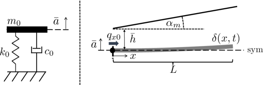
Figure 17: Illustration of spanwise quasi-1D geometry for comparison to experimental results.

To summarize, the separation bubble over the diffusing channel walls effectively serve as a secondary diffuser boundary at an effective expansion angle of $\alpha_{m}<\theta$. The pressure distribution on the beam surface behaves as if the flow had been attached and expanding at $\alpha_{m}$. At the end of the effective diffuser expansion ($x=L$), we assume that the outlet boundary pressure variation behaves as an abrupt expansion at the outlet, where $\zeta_{\mathrm{out}}=1$.

5.5 Model-experiment comparison

We now use the model to assess critical parameters at the on-set of flutter. Critical flow rates and frequencies are calculated over integer values of $\alpha_{m}=[1-8]^{\circ}$ for the flexible Euler-Bernoulli (EB) and a rigid-body (RB) beam formulations. As in pre-cursor numerical simulations, the EB modeled cantilever modes are quickly (or immediately) unstable once flowing in the absence of internal material damping terms. This unphysical behavior precludes their direct comparison to experimental results (i.e. mode 2 in figure 3). However, the EB model still allows us to extract the flexure/flextensional mode where damping has been accounted and experimentally measured, and compare its critical flow rate, frequency, and corresponding shape to those observed experimentally (i.e. mode 1 in figure 3). Hence, only the primary flexure mode is considered for comparison in the EB formulation.

Beginning with critical flow rates, figure 18 shows their calculated values for the EB and RB model formulations compared with experimental values for the three flextensional settings. The corresponding critical frequencies are shown in figure 19. Both model critical flow rate trends are convex, with $\alpha_{\mathrm{m}}\approx 4^{\circ}$ representing the least stable configuration over the diffuser angles tested. $\alpha_{\mathrm{m}}=1^{\circ}$ critical values are not shown for flex. 2 as the mode was stable for tested flow rates ([0-500] L/min). Though EB model critical flow rate values tend to be higher than those predicted by the RB model, they are close to one another at $\alpha_{\mathrm{m}}>3^{\circ}$. Both EB and RB model predictions match experimental critical flow rates near $\alpha_{m}\approx 7^{\circ}$ for all three flextensional settings. This suggests that the critical diffuser angle for plane-asymmetric diffusers may be dictating the flow expansion and pressure distribution over the flow energy harvester channel. Critical frequency trends in figure 19 are largely constant, with a slight increase as $\alpha_{\mathrm{m}}$ increases in both EB and RB models. Predicted frequency values are also close between both model formulations and to those observed experimentally.

Figure 20 shows the unstable EB flexure eigenvectors and experimental SPOD modes closest to the flutter bifurcation point for each of the three flextensional settings. Predicted EB model mode shapes are similar to SPOD modes for flextensional settings 1 and 2, but captures only the rigid body motion, missing the beam shape for flex. 3. The primary motion seen in the modes shown is associated with the translation of the flextensional boundary condition, and are largely captured by the RB formulation.

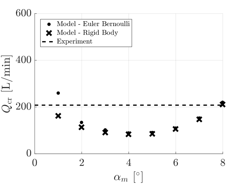
(a) Flex. 1.

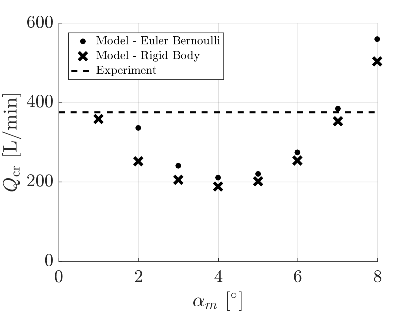
(b) Flex. 2.

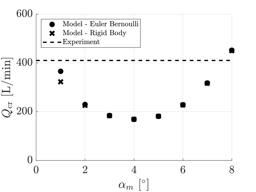
(c) Flex. 3.

Figure 18: Flutter boundary defined by critical flow rate vs. diffuser expansion angle for all three flextensional settings.

(a) Flex. 1.

(b) Flex. 2.

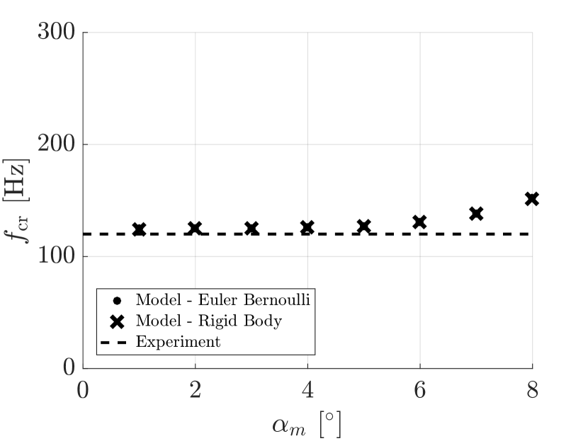
(c) Flex. 3.

Figure 19: Frequencies at critical flow rates vs. diffuser expansion angle for all three flextensional settings.

(a) Flex. 1.

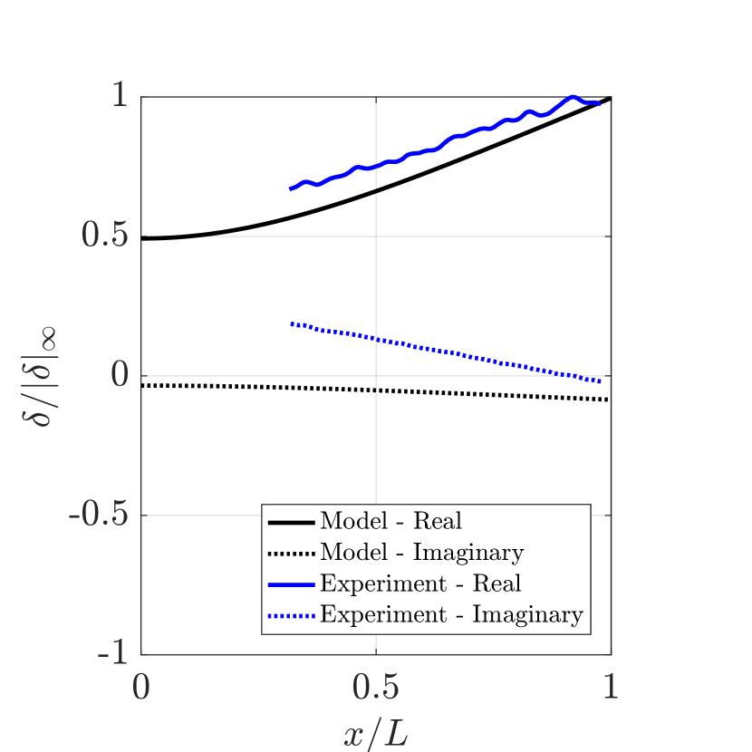
(b) Flex. 2.

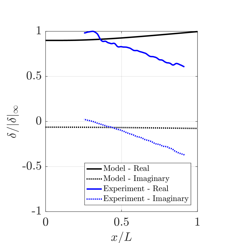
(c) Flex. 3.

Figure 20: Mode shape comparison between Euler-Bernoulli model and experimental SPOD results.

6 Conclusions

This paper explored the fluid-structure instability that drives the dynamics of a flextensional based flow-energy harvester. In particular, we sought to elucidate the mechanisms that drive the system into flutter, which represents the transition between low and high power extraction regimes for the device.

First, we experimentally assessed the dynamics of the flextensional based flow-energy harvester in air flow. Experiments characterized the device’s mechanical properties, then appraised the system dynamics in flowing conditions. Critical flow rates and frequencies were measured for three different flextensional settings, with self-sustaining oscillations reached in the flextensional mode (translational motion at the base of the beam) in all three cases tested. Hysteresis was observed as the flow rate direction is reversed, indicating a bi-stable region and a subcritical Hopf bifurcation at the critical point, also in all three settings.

Numerical simulations were then carried out in three-dimensions to characterize the flow field and edify the experimentally observed flutter. Structure equations for a rigid beam were coupled with a lattice-Boltzmann flow solver to characterize the motion of the flextensional base, and any ensuing coherent structures within the velocity field. The incompressible formulation of flow equations and rigid body structure were able to replicate the critical point and the bi-stable region of the subcritical Hopf bifurcation. Results showed that the flow rate modulation due to confinement at the channel throat largely drives the velocity fluctuations observed at downstream stations. They pointed at a confinement based instability where flow compressibility does not play a significant role.

Finally, an incompressible quasi-one dimensional fluid-structure model based on flow rate modulation due to confinement in the axial and spanwise directions was developed. Flow equations were derived for small throat-to-beam length ratios and defined the pressure on the structure surface as a function of beam displacement and velocity. Results showed that the flutter on-set is captured for a linear diffuser channel, matching experimental values near the typical separation angle for plane-asymmetric diffusers of $7^{\circ}$. The resulting model mode shapes agreed well with experimental SPOD modes for two of the three flextensinal settings tested, with all three capturing the primary base translation motion.

We believe that this work provides tantalizing evidence that the positive feedback between beam displacement (and velocity) and the flow modulation due to confinement is likely the dominant mechanism that drives the flutter instability within the flextensional flow energy harvester system. Flow compressibility and beam flexibility do not appear to significantly impact the fluid-structure dynamics on the current design. Agreement between model-predicted critical properties and experimental results suggest that the framework developed can be used to assess not only future flow energy harvester designs, but fluid-structure systems where small throat-to-beam length dominate the dynamics.

Declaration of interests

The authors report no conflict of interest.

Appendix A Dimension, Material, and Measurement Tables

Table 5 shows dimensions associated with the flextensional design highlighted in figure 1.

Table 5: Table of flow path parameter dimensions illustrated in figure 1.

Variable	Value	Units
$L_{1}$	70	mm
$L_{2}$	5	mm
$L_{3}$	19.4	mm
$L$	40.7	mm
$h_{1}$	9.8	mm
$h_{2}$	2.3	mm
$h_{3}$	9	mm
$\bar{h}$	0.62	mm
$b$	14	mm
$b_{1}$	16.5	mm
$h_{b}$	0.7	mm
$\theta$	19	deg

Material and electrical properties for flexure and PZT stacks are shown in tables 6 and 7.

Table 6: Table of structural material properties (MatWeb, 2018; Boston Piezo Optics Inc., 2018).

Variable	Aluminum	Steel	PZT
Density [kg/m3]	2700	8000	7500
Young’s modulus [GPa]	68.9	193	64.5
Poisson’s ratio [ND]	0.33	0.29	0.31

Table 7: Table of relevant piezoelectric stack properties.

Variable	Value	Units	Description
$C_{p}^{*}$	3.6	$\mu$F	stack capacitance
$K_{s}$	2.8E7	N/m	stack stiffness in 33 mode
$L_{s}\times W_{s}\times H_{s}$	5x5x36	mm	dimensions
$R_{e}$	68	k$\Omega$	circuit resistor
$\tau$	0.245	s	RC time constant
$D_{\mathrm{m}}$	40	$\mu$m	maximum displacement

Results from the static displacement-force and dynamic tests for three flextensional configurations are shown in tables 8 9.

Table 8: Table of mean force [N] at different displacement values for three flexure settings, with a linear best fit slope describing the stiffness $k_{0}$ [N/m].

$\bar{a}$ [mm]	Flex. 1 $F_{a}$ [N]	Flex. 2 $F_{a}$ [N]	Flex 3 $F_{a}$ [N]
0	0	0	0
0.127	4.86	5.40	2.80
0.254	9.12	10.04	5.44
0.381	14.44	16.00	8.24
$k_{0}$ [N/m]	3.73E4	4.12E4	2.16E4

Table 9: Table of experimental flexure values for flexure dynamic test.

Variable	Flex. 1	Flex. 2	Flex. 3
$\omega$ - mean [rad/s]	1167.6	1423.1	767.7
$\omega$ - STD [rad/s]	0.348	4.055	18.821
$\zeta$ - mean [1/s]	-2.471	-7.718	-3.834
$\zeta$ - STD [1/s]	0.071	0.076	0.271

Appendix B Compressibility at Critical Flow Rates

Given $Q_{\mathrm{cr}}$ results in table 10, it is plausible that throat velocities may reach a considerable fraction of the sound speed. To assess whether the critical flow rates may present compressible effects, we estimate the Mach number at the channel throat $\mathcal{M}_{\mathrm{t}}$. Assuming the flow accelerates isentropically over the converging section of the flow path in figure 1 ($x\leq L_{2}$), we take isentropic relations for stagnation (subscript $\mathrm{o}$) and throat (subscript $\mathrm{t}$) quantities,

$$\frac{T_{o}}{T_{t}}=1+\frac{\gamma_{g}-1}{2}\mathcal{M}_{\mathrm{t}}^{2},$$ (62)

$$\frac{\rho_{o}}{\rho_{t}}=\left(1+\frac{\gamma_{g}-1}{2}\mathcal{M}_{\mathrm{t}}^{2}\right)^{\frac{1}{\gamma_{g}-1}},$$ (63)

$$\mathcal{M}_{\mathrm{t}}=\frac{U_{\mathrm{cr}}}{\sqrt{\gamma_{\mathrm{g}}R_{\mathrm{g}}T_{\mathrm{t}}}},$$ (64)

where $R_{\mathrm{g}}$ is the specific gas constant, $\gamma_{\mathrm{g}}$ is the ratio of specific heats, $T$ is the temperature, and $\rho$ is the density. With the definition of the critical mass flow rates as

$$\dot{m}_{\mathrm{cr}}=\rho_{\mathrm{STP}}Q_{\mathrm{cr}}=\rho_{t}A_{\mathrm{t}}U_{\mathrm{cr}},$$ (65)

we can combine equations 62, 63, and 64 to represent an implicit relation between the fluid flow properties and $\mathcal{M}_{\mathrm{t}}$ valid for $\mathcal{M}_{\mathrm{t}}\leq 1$,

$$\frac{\dot{m}_{\mathrm{cr}}}{\sqrt{\frac{\gamma_{g}R_{g}T_{o}}{1+\frac{\gamma_{g}-1}{2}\mathcal{M}_{\mathrm{t}}^{2}}}\mathcal{M}_{\mathrm{t}}A_{\mathrm{t}}}=\frac{\rho_{o}}{\left(1+\frac{\gamma_{g}-1}{2}\mathcal{M}_{\mathrm{t}}^{2}\right)^{\frac{1}{\gamma_{g}-1}}}.$$ (66)

Values for $T_{o}=T_{\mathrm{STP}}=295$ [K], $\rho_{o}=\rho_{\mathrm{STP}}=1.20$ [kg/m³], $R_{\mathrm{g}}=287.0$ [kg/J/K], $\gamma_{\mathrm{g}}=1.40$ (per (Moran & Shapiro, 2004)) and

$$A_{t}=b_{1}(2\bar{h}+h_{b})-bh_{b}$$ (67)

as the throat flow area . Table 10 lists results of $\mathcal{M}_{\mathrm{t}}$ in the three flextensional settings.

Table 10: Table of critical values for flexure settings listed.

Critical Properties	Flex. 1	Flex. 2	Flex. 3	Description
$Q_{\mathrm{cr}}$ [L/min]	208	376	410	critical flow rate
$\mathcal{M}_{\mathrm{t}}$	0.53	1	1	throat Mach number est.

The chocked flow rate is $Q_{\mathrm{ch}}\approx 267$ [L/min] for flow path with dimensions in table 5. $\mathcal{M}_{\mathrm{t}}$ values suggest that flextensional settings 2 and 3 are chocked, while flextensinal 1 is not. The possibility of having $Q_{\mathrm{cr}}>Q_{\mathrm{ch}}$ for the former two settings is due to the increase in stagnation pressure downstream of the needle valve: the flow meter measurements represent a mass flow rate rather than a purely volumetric one. Since the flow control (needle) valve is upstream of the flow meter and the test section, by further opening the valve, the upstream flowing and stagnation pressures are increased, which in turn increase the density at throat and allows for the higher mass flow rate through the system. This happens despite the volumetric flow rate remaining constant in the choked condition.

Appendix C Spectral Proper Orthogonal Decomposition

To define the spectral proper orthogonal decomposition, we choose the transverse displacement $\delta$ as the primary quantity to characterize the fluid-structure system dynamics. The inertial coordinate $x$ spans the length of the beam, with $y$ displacement at discrete $x_{i}$ ($i\in\mathbb{Z}:[1,p]$) and time $t_{j}$ ($j\in\mathbb{Z}:[1,n]$ ) as $\delta(x_{i},t_{j})=\delta^{(j)}_{i}$. We define the data matrix $\mathbf{X}$,

$$\mathbf{X}=\begin{bmatrix}\delta_{1}^{(1)}&\delta_{1}^{(j)}&\dots&\delta_{1}^{(n)}\\ \delta_{i}^{(1)}&\delta_{i}^{(j)}&\dots&\delta_{i}^{(n)}\\ \vdots&\vdots&\ddots&\vdots\\ \delta_{p}^{(1)}&\delta_{p}^{(j)}&\dots&\delta_{p}^{(n)}\end{bmatrix}\in\mathbb{R}^{p\times n}.$$ (68)

The rows of $\mathbf{X}$ are measurements of points along the beam, and the columns are the time series for each point with size $\Delta t$.

Assuming that the system is stationary and consistent with the procedure in (Towne et al., 2018; Schmidt & Towne, 2019), the DFT of each row of our $\mathbf{X}$ is carried out using Welch’s method (Welch, 1967). In the procedure, each discrete time series is segmented into 50% overlapping blocks of size $n_{f}\leq n$, Fourier transformed, and assembled into a Fourier domain data matrix $\tilde{\mathbf{X}}_{f_{l}}$ at each discrete frequency $f_{l}$,

$$\tilde{\mathbf{X}}_{f_{l}}=\begin{bmatrix}\tilde{\delta}_{1}^{(1)}&\tilde{\delta}_{1}^{(k)}&\dots&\tilde{\delta}_{1}^{(N)}\\ \tilde{\delta}_{i}^{(1)}&\tilde{\delta}_{i}^{(k)}&\dots&\tilde{\delta}_{i}^{(N)}\\ \vdots&\vdots&\ddots&\vdots\\ \tilde{\delta}_{p}^{(1)}&\tilde{\delta}_{p}^{(k)}&\dots&\tilde{\delta}_{p}^{(N)}\end{bmatrix}_{f_{l}}\in\mathbb{C}^{p\times N},$$ (69)

where $l\in\mathbb{Z}:[1,n_{f}]$, $N\geq 1\in\mathbb{Z}$ is the total number of blocks in Welch’s method, $k\in\mathbb{Z}:[1,N]$ is a Fourier realization of the data and block number index. Elements in $\tilde{\mathbf{X}}_{f_{l}}$ are

$$\tilde{\delta}_{i}^{(k)}=\frac{1}{\sqrt{n_{f}}}\sum_{j=\frac{n_{f}}{2}\left(k-1\right)+1}^{\frac{n_{f}}{2}\left(k+1\right)}\delta_{i}^{(j)}\text{e}^{-2\pi\sqrt{-1}\left(l-1\right)\frac{j-1}{n_{f}}},$$ (70)

for a rectangular windowing function, and discrete frequencies

$$f_{l}=\begin{cases}\frac{l-1}{n_{f}\Delta t}&\text{for }l\leq n_{f}/2\\ \frac{l-1-n_{f}}{n_{f}\Delta t}&\text{for }l>n_{f}/2\end{cases}.$$ (71)

We build the cross-spectral density matrix at each $f_{l}$,

$$\tilde{\mathbf{S}}_{f_{l}}=\frac{\Delta t}{n_{f}N}\tilde{\mathbf{X}}_{f_{l}}\tilde{\mathbf{X}}_{f_{l}}^{*}\in\mathbb{C}^{p\times p},$$ (72)

where $\tilde{\mathbf{X}}_{f_{l}}^{*}$ is the conjugate transpose of $\tilde{\mathbf{X}}_{f_{l}}$ and $\Delta t$ is the time increment for the series. $\tilde{\mathbf{S}}_{f_{l}}$ is Hermitian and represents the cross-correlation of measurement $i$ Fourier coefficients with all other measurements, averaged over all realizations. We can eigendecompose $\tilde{\mathbf{S}}_{l}$,

$$\tilde{\mathbf{S}}_{l}=\hat{\mathbf{U}}_{l}\bm{\Sigma}_{l}\hat{\mathbf{U}}_{l}^{*}$$ (73)

where $\hat{\mathbf{U}}_{l}$ is unitary (along with its conjugate transpose $\hat{\mathbf{U}}_{l}^{*}$) and its columns $(\hat{\mathbf{u}}_{i})_{l}$ are orthonormal eigenvectors of $\tilde{\mathbf{S}}_{l}$. $\bm{\Sigma}_{l}\in\mathbb{R}^{p\times p}$ is a diagonal matrix with its entries as the eigenvalues $(\sigma_{i})_{l}$ in descending order. $(\sigma_{i})_{l}$ can be interpreted as the amount of energy its pair $(\hat{\mathbf{u}}_{i})_{l}$ contains at $f_{l}$. The cross-spectral density at each $f_{l}$ is tensor invariant tr$(\hat{\mathbf{S}}_{l})=\text{tr}\left(\bm{\Sigma}_{l}\right)$, and represents the total energy at each frequency. The fraction of energy each mode contains is

$$\left(\hat{\sigma}_{i}\right)_{l}=\frac{\left(\sigma_{i}\right)_{l}}{\text{tr}(\hat{\bm{\Sigma}}_{l})}.$$ (74)

The system may be reduced further if a single $\left(\hat{\sigma}_{i}\right)_{l}$, $(\hat{\mathbf{u}}_{i})_{l}$ pair contains most of the energy at these peak frequencies. In systems where both holds true, it is often useful to understand the dynamics of these predominant modes. Frequencies where $\text{tr}(\hat{\bm{\Sigma}}_{l})$ peaks indicate periodic behavior, but do not discern between periodic oscillations characteristic of a limit-cycle, or intermittent periodic behavior associated with a stochastically forced under-damped system. However, the SPOD modes provide a means to filter the original time domain data and discern those states exactly. In (Schmidt et al., 2017) first explored this by projecting time domain pressure data onto the leading SPOD modes to find intermittent behavior of noise in a turbulent jet. Here, we would like to do the same by projecting the time domain beam displacement data onto the leading SPOD beam shapes.

Suppose the system has $m<n_{f}$ peak frequencies in $\text{tr}(\hat{\bm{\Sigma}}_{l})$. To explore the time behavior of the most energetic modes at each peak frequency, we build a basis,

$$\hat{\bm{\Phi}}=\big{[}(\hat{\mathbf{u}}_{1})_{1},\cdots,(\hat{\mathbf{u}}_{1})_{m}\big{]}\in\mathbb{C}^{p\times m},$$ (75)

where subscript 1 in $\hat{\mathbf{u}}_{1}$ indicates the leading mode. We would like to approximate the time domain data $\mathbf{X}$ as

$$\mathbf{X}\approx\hat{\bm{\Phi}}\mathbf{A}$$ (76)

where $\mathbf{A}$ is the matrix with coefficients of each basis (rows) in $\hat{\bm{\Phi}}$ over time (columns). To solve for $\mathbf{A}$,

$$\mathbf{A}=\left(\hat{\bm{\Phi}}^{*}\hat{\bm{\Phi}}\right)^{-1}\hat{\bm{\Phi}}^{*}\mathbf{X}.$$ (77)

where $\hat{\bm{\Phi}}^{*}$ is the conjugate transpose of $\hat{\bm{\Phi}}$. The columns of $\hat{\bm{\Phi}}$ are not orthogonal, and $\left(\hat{\bm{\Phi}}^{*}\hat{\bm{\Phi}}\right)^{-1}$ accounts for the cross-coupling between the modes. By construction, modes are orthonormal within a single frequency, but not across frequencies when only considering the spatial norm.

The map between $\mathbf{A}$ and $\mathbf{X}$ is, in essence, a spatial filter that when applied to the time-domain data elucidates how each shape $\hat{\mathbf{u}}_{1}$ behaves in time. With $\mathbf{X}$ built as transverse displacement $\delta_{p}^{(j)}$, each basis in $\hat{\bm{\Phi}}$ represents a beam mode shape and the columns of $\mathbf{A}$ their amplitudes at a particular instance in time.

Since $\mathbf{A}$ represents beam displacement over time, the velocity of each shape can be defined as $\frac{\mathrm{d}\mathbf{A}}{\mathrm{d}t}$ and estimated through a discrete time derivative for the data set. We can access a two-dimensional phase-portrait of each mode, and discern their individual dynamics: periodic orbits will be closed orbits (donut shape), while amplifier states as points clumped around the origin, as the mode is perturbed stochastically, but decays back to its equilibrium.

Appendix D Euler-Bernoulli Beam Fundamental Frequency

From classical Euler-Bernoulli beam theory, we can calculate the theoretical clamped-free beam frequencies as

$$f_{i}=\frac{\left(\beta_{i}L\right)^{2}}{2\pi L^{2}}\sqrt{\frac{EI}{\rho_{s}bh_{b}}}.$$ (78)

$I$ is the square cross-section moment of inertia for the beam in three dimensions,

$$I=\frac{h_{b}^{3}b}{12}.$$ (79)

The eigenfunctions $\phi_{k}$, $k\in\mathbb{Z}:[1,\infty]$, when subject to the clamped-free boundary conditions, are

$$\phi_{k}(x)=\cosh\!\left(\beta_{k}\,x\right)-\cos\!\left(\beta_{k}\,x\right)+\left[\frac{\cos\!\left(\beta_{k}\,{L}\right)+\cosh\!\left(\beta_{k}\,{L}\right)}{\sin\!\left(\beta_{k}\,{L}\right)+\sinh\!\left(\beta_{k}\,{L}\right)}\right]\Big{(}\sin\!\left(\beta_{k}\,x\right)\,-\sinh\!\left(\beta_{k}\,x\right)\,\Big{)},$$ (80)

with characteristic equation

$$\cosh\left(\beta_{k}L\right)\cos\left(\beta_{k}L\right)+1=0.$$ (81)

The first six corresponding eigenvalues are listed in table 11

Table 11: Table of solutions to the characteristic equation for clamped-free Euler-Bernoulli Beam.

$\beta_{1}L$	$\beta_{2}L$	$\beta_{3}L$	$\beta_{4}L$	$\beta_{5}L$	$\beta_{6}L$
1.8751	4.6941	7.8548	10.9955	14.1372	17.2788

Appendix E Fluid-structure coefficients

$$\mathbf{A}=\mathbf{\begin{bmatrix}0&\mathbf{1}&0&0\\ M^{-1}K&M^{-1}C&M^{-1}T&M^{-1}H\\ E_{\mathrm{q}}+B_{\mathrm{q}}(M^{-1}K)&D_{\mathrm{q}}+B_{\mathrm{q}}(M^{-1}C)&G_{\mathrm{q}}+B_{\mathrm{q}}(M^{-1}T)&H_{\mathrm{q}}+B_{\mathrm{q}}(M^{-1}H)\\ \tilde{E}_{\mathrm{q}}+\tilde{B}_{\mathrm{q}}(M^{-1}K)&\tilde{D}_{\mathrm{q}}+\tilde{B}_{\mathrm{q}}(M^{-1}C)&\tilde{G}_{\mathrm{q}}+\tilde{B}_{\mathrm{q}}(M^{-1}T)&\tilde{H}_{\mathrm{q}}+\tilde{B}_{\mathrm{q}}(M^{-1}H)\end{bmatrix}}$$ (82)

where,

$${M}_{\mathrm{s}i}=\begin{cases}\frac{m_{0}}{b}&\text{for }i=0\\ \rho_{s}h_{b}g_{i}(x)&\text{for }i=[1,n]\end{cases},$$ (83)

$${C}_{\mathrm{s}i}=\begin{cases}\frac{c_{0}}{b}&\text{for }i=0\\ 0&\text{for }i=[1,n]\end{cases},$$ (84)

$${K}_{\mathrm{s}i}=\begin{cases}\frac{k_{0}}{b}&\text{for }i=0\\ \frac{EI}{b}\frac{\mathrm{d}^{4}}{\mathrm{d}x^{4}}g_{i}(x)&\text{for }i=[1,n]\end{cases}.$$ (85)

and

$$M_{ji} =\int_{0}^{L}\left(M_{\mathrm{s}i}(x)+2M_{\mathrm{f}i}(x)\right)g^{\prime}_{j}(x)dx,\ C_{ji}=-\int_{0}^{L}\left(C_{\mathrm{s}i}(x)+2C_{\mathrm{f}i}(x)\right)g^{\prime}_{j}(x)dx,$$ (86)

$$K_{ji} =-\int_{0}^{L}\left(K_{\mathrm{s}i}(x)+2K_{\mathrm{f}i}(x)\right)g^{\prime}_{j}(x)dx,\$$

exist in $\mathbb{R}^{n+1\ \times\ n+1}$,

$$T_{j}=-2\int_{0}^{L}T_{\mathrm{f}}(x)g^{\prime}_{j}(x)dx,\$$ (87)

exists in $\mathbb{R}^{n+1\ \times\ 1}$, and

$$H_{ji}=-2\int_{0}^{L}H_{\mathrm{f}i}(x)g^{\prime}_{j}(x)dx,\$$ (88)

exists in $\mathbb{R}^{n+1\ \times\ m+1}$. The test functions are

$$g^{\prime}_{i}(x)=\begin{cases}\delta(x)&\text{for }i=0\\ \phi_{i}(x)&\text{for }i=[1,n]\end{cases},$$ (89)

where $\delta$ is the Dirac delta function and $\phi_{i}$ is defined in 80. Coefficients for the spanwise terms

$$\tilde{B}_{\mathrm{q}ji} =N_{ji}\int_{0}^{L}B_{\mathrm{q}i}(x)\psi^{\prime}_{j}(x)dx,\ \tilde{D}_{\mathrm{q}ji}=N_{ji}\int_{0}^{L}D_{\mathrm{q}i}(x)\psi^{\prime}_{j}(x)dx,$$ (90)

$$\tilde{E}_{\mathrm{q}ji} =N_{ji}\int_{0}^{L}E_{\mathrm{q}i}(x)\psi^{\prime}_{j}(x)dx,\ \tilde{G}_{\mathrm{q}ji}=N_{ji}\int_{0}^{L}G_{\mathrm{q}i}(x)\psi^{\prime}_{j}(x)dx,$$

$$\tilde{H}_{\mathrm{q}ji} =N_{ji}\int_{0}^{L}H_{\mathrm{q}i}(x)\psi^{\prime}_{j}(x)dx,\ N_{ji}=\left(\int_{0}^{L}\psi^{\prime}_{i}(x)\psi^{\prime}_{j}(x)dx\right)^{-1}.$$

The test functions are

$$\psi^{\prime}_{i}(x)=\begin{cases}\delta(x)&\text{for }i=0\\ \tilde{\psi}_{i}(x)&\text{for }i=[1,m-1]\\ \delta(x-L)&\text{for }i=m\\ \end{cases},$$ (91)

where $\delta$ is the Dirac delta function and $\tilde{\psi}$ is defined in equation 56.

References

- Alben (2008) Alben, S. 2008 Optimal flexibility of a flapping appendage in an inviscid fluid. Journal of Fluid Mechanics 614, 355–380.
- Alben (2015) Alben, S. 2015 Flag flutter in inviscid channel flow. Physics of Fluids 27 (3), 033603.
- Backus (1963) Backus, J. 1963 Small-vibration theory of the clarinet. The Journal of the Acoustical Society of America 35 (3), 305–313.
- Balint & Lucey (2005) Balint, T. S. & Lucey, A. D. 2005 Instability of a cantilevered flexible plate in viscous channel flow. Journal of Fluids and Structures 20 (7 SPEC. ISS.), 893–912.
- Banks & Inman (1991) Banks, H. T. & Inman, D. J. 1991 On damping mechanisms in beams. Journal of Applied Mechanics 58 (3), 716–723.
- Bastiaanssen et al. (2000) Bastiaanssen, W. G. M., Molden, D. J. & Makin, I. W. 2000 Remote sensing for irrigated agriculture: examples from research and possible applications. Agricultural Water Management 46, 137–155.
- Bernitsas et al. (2008) Bernitsas, M. M., Raghavan, K., Ben-Simon, Y. & Garcia, E. M. 2008 Vivace (vortex induced vibration aquatic clean energy): a new concept in generation of clean and renewable energy from fluid flow. Journal of Offshore Mechanics and Arctic Engineering 130 (4), 041101.
- Bösch et al. (2015a) Bösch, F., Chikatamarla, S. S. & Karlin, I. V. 2015a Entropic multirelaxation lattice Boltzmann models for turbulent flows. Phys. Rev. E 92 (4), 43309.
- Bösch et al. (2015b) Bösch, F., Chikatamarla, S. S. & Karlin, I. V. 2015b Entropic multirelaxation models for simulation of fluid turbulence. ESAIM. Proceedings and Surveys 52, 1–24.
- Boston Piezo Optics Inc. (2018) Boston Piezo Optics Inc. 2018 Ceramic materials. https://www.bostonpiezooptics.com/ceramic-materials-pzt, Used for PZT-5H properties. Accessed: 2018-06-30.
- Canny (1986) Canny, J. 1986 A computational approach to edge detection. IEEE Transactions on pattern analysis and machine intelligence (6), 679–698.
- Chandavari & Palekar (2014) Chandavari, V. & Palekar, S. 2014 Diffuser angle control to avoid flow separation. Int. J. Tech. Res. Appl 2 (5), 16–21.
- Chen et al. (2003) Chen, H., Kandasamy, S., Orszag, S., Shock, R., Succi, S. & Yakhot, V. 2003 Extended Boltzmann kinetic equation for turbulent flows. Science 301 (5633), 633–636.
- Cisonni et al. (2017) Cisonni, J., Lucey, A. D., Elliott, N. S.J. & Heil, M. 2017 The stability of a flexible cantilever in viscous channel flow. Journal of Sound and Vibration 396, 186–202.
- Doaré et al. (2011-B) Doaré, O., Mano, D., Carlos, J. & Ludena, B. 2011-B Effect of spanwise confinement on flag flutter: Experimental measurements. Physics of Fluids pp. 1–4.
- Doaré et al. (2011-A) Doaré, O., Sauzade, M. & Eloy, C. 2011-A Flutter of an elastic plate in a channel flow: Confinement and finite-size effects. Journal of Fluids and Structures 27 (1), 76–88.
- Doll et al. (2010) Doll, G. L., Kotzalas, M. N. & Kang, Y. S. 2010 Life-limiting wear of wind turbine gearbox bearings: origins and solutions. Proceedings of European wind energy conference exhibition (EWEC 2010) 4.
- Dorschner et al. (2016) Dorschner, B., Bösch, F., Chikatamarla, S. S., Boulouchos, K. & Karlin, I. V. 2016 Entropic multi-relaxation time lattice Boltzmann model for complex flows. Journal of Fluid Mechanics 801, 623–651.
- Dorschner et al. (2015) Dorschner, B., Chikatamarla, S. S., Bösch, F. & Karlin, I. V. 2015 Grad’s approximation for moving and stationary walls in entropic lattice Boltzmann simulations. Journal of Computational Physics 295, 340–354.
- Dorschner et al. (2017a) Dorschner, B., Chikatamarla, S. S. & Karlin, I. V. 2017a Entropic multirelaxation-time lattice Boltzmann method for moving and deforming geometries in three dimensions. Physical Review E 95 (6), 063306.
- Dorschner et al. (2017b) Dorschner, B., Chikatamarla, S. S. & Karlin, I. V. 2017b Transitional flows with the entropic lattice Boltzmann method. Journal of Fluid Mechanics 824, 388–412.
- Dorschner et al. (2018) Dorschner, B., Chikatamarla, S. S. & Karlin, I. V. 2018 Fluid-structure interaction with the entropic lattice Boltzmann method. Physical Review E 97 (2), 023305.
- Fujita & Shintani (1999) Fujita, K. & Shintani, A. 1999 Flow-induced vibration of the elastic rod due to axial flow: unstable phenomena of continuous flexible rod as the axisymmetric body. PVP Flow Induced Vibration 389, 199–206.
- Fujita & Shintani (2001) Fujita, K. & Shintani, A. 2001 Axial Leakage Flow-Induced Vibration of the Elastic Rod as the Axisymmetric Continuous Flexible Beam. Journal of Pressure Vessel Technology 123 (4), 421.
- Fujita & Shintani (2007) Fujita, K. & Shintani, A. 2007 A consideration on pre- and post-instability of an axisymmetric elastic beam subjected to axial leakage flow. Journal of Fluids and Structures 23 (3), 463–478.
- Guo & Paidoussis (2000) Guo, C. Q. & Paidoussis, M. P. 2000 Stability of rectangular plates with free side-edges in two-dimensional inviscid channel flow. Journal of Applied Mechanics 67 (1), 171–176.
- Guo et al. (2009) Guo, H., Watson, S., Tavner, P. & Xiang, J. 2009 Reliability analysis for wind turbines with incomplete failure data collected from after the date of initial installation. Reliability Engineering & System Safety 94 (6), 1057–1063.
- Gurugubelli & Jaiman (2019) Gurugubelli, P. S. & Jaiman, R. K. 2019 Interaction of gap flow with flapping dynamics of two side-by-side elastic foils. International Journal of Heat and Fluid Flow 75, 239–255.
- Gurugubelli et al. (2014) Gurugubelli, P. S., Jaiman, R. K. & Khoo, B. C. 2014 Flexible flapping dynamics of parallel elastic plates in a uniform flow: application to energy harvesting devices. International Conference on Offshore Mechanics and Arctic Engineering 45400, V002T08A038.
- Hidalgo et al. (2015) Hidalgo, P., Jha, S. & Glezer, A. 2015 Enhanced heat transfer in air cooled heat sinks using aeroelastically fluttering reeds. In Thermal Investigations of ICs and Systems (THERMINIC), 2015 21st International Workshop on, pp. 1–6. IEEE.
- Inada & Hayama (1988) Inada, F. & Hayama, S. 1988 A Study on Leakage-Flow-Induced Vibrations. Japan Society of Mechanical Engineers International Journal Ser. 3, Vibration, Control Engineering, Engineering for Industry 31 (1), 39–47.
- Inada & Hayama (1990) Inada, F. & Hayama, S. 1990 A study on leakage-flow-induced vibrations. Part 1: Fluid-dynamic forces and moments acting on the walls of a narrow tapered passage. Journal of Fluids and Structures 4 (4), 395–412.
- Inman (2008) Inman, D. J. 2008 Distributed-parameter systems. In Engineering vibration, , vol. 3, chap. 6, pp. 464–538. Prentice Hall New Jersey.
- Jaiman et al. (2014) Jaiman, R. K., Parmar, M. K. & Gurugubelli, P. S. 2014 Added mass and aeroelastic stability of a flexible plate interacting with mean flow in a confined channel. Journal of Applied Mechanics 81 (4).
- Johansson (1959) Johansson, E. B. 1959 Hydraulic instability of reactor parallel-plate fuel assemblies. Tech. Rep.. Knolls Atomic Power Lab., Schenectady, NY.
- Kaltenbach et al. (1999) Kaltenbach, H. J., Fatica, M., Mittal, R., Lund, T. S. & Moin, P. 1999 Study of flow in a planar asymmetric diffuser using large-eddy simulation. Journal of Fluid Mechanics 390, 151–185.
- Karlin et al. (2014) Karlin, I. V., Bösch, F. & Chikatamarla, S. S. 2014 Gibbs’ principle for the lattice-kinetic theory of fluid dynamics. Physical Review E 90 (3), 031302.
- Kundu et al. (2012) Kundu, P. K., Cohen, I. & Dowling, D. R. 2012 Fluid mechanics. Elsevier.
- Lan et al. (2009) Lan, H., Armaly, B. F. & Drallmeier, J. A. 2009 Turbulent forced convection in a plane asymmetric diffuser: Effect of diffuser angle. Journal of Heat Transfer 131 (7), 071702.
- Lee et al. (2016) Lee, H. J., Sherrit, S., Tosi, L. P. & Colonius, T. 2016 Design and experimental evaluation of flextensional-cantilever based piezoelectric transducers for flow energy harvesting. In SPIE Smart Structures and Materials + Nondestructive Evaluation and Health Monitoring. International Society for Optics and Photonics.
- Lee et al. (2015) Lee, H. J., Sherrit, S., Tosi, L. P., Walkemeyer, P. & Colonius, T. 2015 Piezoelectric energy harvesting in internal fluid flow. Sensors 15 (10).
- Malaspinas & Sagaut (2012) Malaspinas, O. & Sagaut, P. 2012 Consistent subgrid scale modelling for lattice Boltzmann methods. Journal of Fluid Mechanics 700, 514–542.
- MatWeb (2018) MatWeb 2018 Material Property Data. http://matweb.com/search/DataSheet.aspx?MatGUID=b8d536e0b9b54bd7b69e4124d8f1d20a&ckck=1, Used for aluminum and steel properties. Accessed: 2018-06-30.
- Miller (1960) Miller, D. R. 1960 Critical flow velocities for collapse of reactor parallel-plate fuel assemblies. Journal of Engineering for Power 82 (2), 83–91.
- Moran & Shapiro (2004) Moran, M. J. & Shapiro, H. N. 2004 Fundamentals of engineering thermodynamics. John Wiley & Sons.
- Moschitta & Neri (2014) Moschitta, A. & Neri, I. 2014 Power consumption assessment in wireless sensor networks. ICT-Energy-Concepts Towards Zero-Power Information and Communication Technology .
- Nagakura & Kaneko (1991) Nagakura, H. & Kaneko, S. 1991 The stability of a cantilever beam subjected to one-dimensional leakage flow. Transactions of the 11th international conference on structural mechanics in reactor technology .
- Païdoussis (2003) Païdoussis, M. P. 2003 Annular- and Leakage- Flow-Induced Instabilities. In Fluid-Structure Interactions: Slender Structures and Axial Flow, Volume 2, chap. 11, pp. 1221–1420. Academic Press.
- Rester et al. (1999) Rester, S., Thomas, J., Hilten, M. P. V. & Vidrine, W. L. 1999 Application of intelligent completion technology to optimize the reservoir management of a deepwater gulf of mexico field: a reservoir simulation case study. In SPE annual technical conference, pp. 573–581.
- Schmidt et al. (2017) Schmidt, O. T., Colonius, T. & Bres, G. A. 2017 Wavepacket intermittency and its role in turbulent jet noise. 55th AIAA Aerospace Sciences Meeting p. 0686.
- Schmidt et al. (2018) Schmidt, O. T., Schmid, P. J., Towne, A. & Lele, S. K. 2018 Statistical description of intermittency and rare events via conditional space-time pod: Example of acoustic bursts in turbulent jets. Center for Turbulence Research Annual Research Briefs .
- Schmidt & Towne (2019) Schmidt, Oliver T & Towne, Aaron 2019 An efficient streaming algorithm for spectral proper orthogonal decomposition. Computer Physics Communications 237, 98–109.
- Sharma et al. (2002) Sharma, A. K., Chorn, L. G., Han, J., Rajagopalan, S. & others 2002 Quantifying value creation from intelligent completion technology implementation. In European Petroleum Conference. Society of Petroleum Engineers.
- Sherrit et al. (2009) Sherrit, S., Frankovich, K., Bao, X. & Tucker, C. 2009 Miniature piezoelectric shaker mechanism for autonomous distribution of unconsolidated sample to instrument cells. In Industrial and Commercial Applications of Smart Structures Technologies, , vol. 7290, pp. 72900H–1 – 72900H–9. International Society for Optics and Photonics.
- Sherrit et al. (2014) Sherrit, S., Lee, H. J., Walkemeyer, P., Hasenoehrl, J., Hall, J. L., Colonius, T., Tosi, L. P., Arrazola, A., Kim, N., Sun, K. & others 2014 Flow energy piezoelectric bimorph nozzle harvester. In SPIE Smart Structures and Materials + Nondestructive Evaluation and Health Monitoring. International Society for Optics and Photonics.
- Sherrit et al. (2015) Sherrit, S., Lee, H. J., Walkemeyer, P., Winn, T., Tosi, L. P. & Colonius, T. 2015 Fluid flow nozzle energy harvesters. In SPIE Smart Structures and Materials + Nondestructive Evaluation and Health Monitoring. International Society for Optics and Photonics.
- Shoele & Mittal (2016) Shoele, K. & Mittal, R. 2016 Flutter instability of a thin flexible plate in a channel. Journal of Fluid Mechanics 786, 29–46.
- Sommerfeldt & Strong (1988) Sommerfeldt, S. D. & Strong, W. J. 1988 Simulation of a player–clarinet system. The Journal of the Acoustical Society of America 83 (5), 1908–1918.
- Tetlow & Lucey (2009) Tetlow, G. A. & Lucey, A. D. 2009 Motions of a cantilevered flexible plate in viscous channel flow driven by a constant pressure drop. International Journal for Numerical Methods in Biomedical Engineering 25 (5), 463–482.
- Tian et al. (2014) Tian, F. B., Dai, H., Luo, H., Doyle, J. F. & Rousseau, B. 2014 Fluid–structure interaction involving large deformations: 3d simulations and applications to biological systems. Journal of computational physics 258, 451–469.
- Tong (2010) Tong, W. 2010 Wind power generation and wind turbine design. Wit Press.
- Törnblom et al. (2009) Törnblom, O., Lindgren, B. & Johansson, A. V. 2009 The separating flow in a plane asymmetric diffuser with 8.5 opening angle: mean flow and turbulence statistics, temporal behaviour and flow structures. Journal of Fluid Mechanics 636, 337–370.
- Tosi (2019) Tosi, L. P. 2019 Fluid-structure stability in an internal flow energy harvester. PhD thesis, California Institute of Technology.
- Tosi & Colonius (2019) Tosi, L. P. & Colonius, T. 2019 Modeling and simulation of a fluttering cantilever in channel flow. Journal of Fluids and Structures .
- Towne et al. (2018) Towne, A., Schmidt, O. T. & Colonius, T. 2018 Spectral proper orthogonal decomposition and its relationship to dynamic mode decomposition and resolvent analysis. Journal of Fluid Mechanics 847, 821–867.
- Welch (1967) Welch, P. 1967 The use of fast fourier transform for the estimation of power spectra: a method based on time averaging over short, modified periodograms. IEEE Transactions on audio and electroacoustics 15 (2), 70–73.
- Wen et al. (2015) Wen, B., Zhang, C. & Fang, H. 2015 Hydrodynamic force evaluation by momentum exchange method in lattice Boltzmann simulations. Entropy 17 (12), 8240–8266.
- Wood et al. (2013) Wood, M. H., Arellano, A. L. V. & Lorenzo, V. 2013 Corrosion related accidents in petroleum refineries. European Commission Joint Research Centre .
- Wu & Kaneko (2005) Wu, X. & Kaneko, S. 2005 Linear and nonlinear analyses of sheet flutter induced by leakage flow. Journal of Fluids and Structures 20 (7), 927–948.
- Zhou et al. (2012) Zhou, G., Huang, L., Li, W. & Zhu, Z. 2012 Harvesting ambient environmental energy for wireless sensor networks: a survey 2014.
- Zhu (2011) Zhu, D. 2011 Vibration energy harvesting: machinery vibration, human movement and flow induced vibration. InTech.