Modeling optical roughness and first-order scattering processes from OSIRIS-REx color images of the rough surface of asteroid (101955) Bennu

Abstract

The dark asteroid (101955) Bennu studied by NASA’s OSIRIS-REx mission has a boulder-rich and apparently dust-poor surface, providing a natural laboratory to investigate the role of single-scattering processes in rough particulate media. Our goal is to define optical roughness and other scattering parameters that may be useful for the laboratory preparation of sample analogs, interpretation of imaging data, and analysis of the sample that will be returned to Earth. We rely on a semi-numerical statistical model aided by digital terrain model (DTM) shadow ray-tracing to obtain scattering parameters at the smallest surface element allowed by the DTM (facets of ~10 cm). Using a Markov Chain Monte Carlo technique, we solved the inversion problem on all four-band images of the OSIRIS-REx mission’s top four candidate sample sites, for which high-precision laser altimetry DTMs are available. We reconstructed the a posteriori probability distribution for each parameter and distinguished primary and secondary solutions. Through the photometric image correction, we found that a mixing of low and average roughness slope best describes Bennu’s surface for up to $90^{\circ}$ phase angle. We detected a low non-zero specular ratio, perhaps indicating exposed sub-centimeter mono-crystalline inclusions on the surface. We report an average roughness RMS slope of $27_{-5}^{\circ+1}$, a specular ratio of $2.6_{-0.8}^{+0.1}\%$, an approx. single-scattering albedo of $4.64_{-0.09}^{+0.08}\%$ at 550 nm, and two solutions for the back-scatter asymmetric factor, $\xi^{(1)}=-0.360\pm 0.030$ and $\xi^{(2)}=-0.444\pm 0.020$, for all four sites altogether.

1 Introduction

OSIRIS-REx (Origins, Spectral Interpretation, Resource Identification, and Security–Regolith Explorer) is a NASA mission intended to collect and bring back to Earth a sample of pristine material from the carbonaceous chondrite–like asteroid (101955) Bennu (Lauretta et al., 2017). Arriving at Bennu on December 3, 2018, the mission has performed disk-resolved surface characterization to better understand the asteroid and prepare for the selection of a sample site. The spacecraft’s remote sensing payload includes a VIS camera suite (OCAMS), a scanning laser altimeter (OLA), two point spectrometers (OVIRS and OTES; VIS-NIR and thermal IR, respectively) and an x-ray imaging spectrometer (REXIS).

The initial results from the mission confirmed the presence of an equatorial budge (Scheeres et al., 2019; Barnouin et al., 2020) and aqueously altered minerals with similar compositions to those found in CM carbonaceous chondrites (Hamilton et al., 2019). The OCAMS images showed a dark, boulder-rich environment with an average geometric albedo of $4.4\pm 0.2\%$ at 550 nm. Multiple instruments indicated a lack of widespread micrometric grains (DellaGiustina et al., 2019; Lauretta et al., 2019).

In this work, we study the role of multi-scale roughness, shadowing, and other first-order scattering processes on the surface of Bennu. This asteroid’s dark, boulder-rich, apparently dust-poor surface provides a natural laboratory to investigate the role of single-scattering processes in rough particulate surfaces and their effects on the bi-directional reflectance distribution function (BRDF) or radiance factor (RADF) distribution.

For highly absorbent surfaces observed off the opposition configuration, the RADF distribution is largely controlled by roughness with a characteristic scale much larger than the particle size, i.e., the roughness scale situated in the optical regime. This regime configuration is also known as hierarchically arranged random topography (Shkuratov et al., 2005). On rough surfaces, there are the formation of shadows and occlusions, yielding most of the variation in reflectance of an homogeneous surface observed at varied scattering geometry.

For analytically computing the radiative contribution of the macroscopic roughness, the Hapke shadowing function (Hapke, 1984) has been usually adopted by the planetary science community (Li et al., 2015). However, this function has come under scrutiny for failing to reproduce non-Gaussian topographies (Davidsson et al., 2015; Labarre et al., 2017), poorly scaling for higher roughness slopes (Labarre et al., 2017) and allegedly violating the energy conservation (Shkuratov et al., 2012; Hapke, 2013). To counterpoint these three problems from the Hapke shadowing function, we reintroduce the formalism put forward by van Ginneken et al. (1998), a semi-numerical statistical model that simulates diffuse and specular scattering arising from illuminated Gaussian-random rough surfaces that scales into high roughness slopes. On its first application to astronomical data, Goguen et al. (2010) adapted the model to use the Lommel-Seeliger law, and it was successfully applied to ROLO (Robotic Lunar Observatory) photometric data of the Moon. The results showed generally good agreement with the Hapke model, but with a more pronounced optical roughness for the Lunar Highlands (Helfenstein & Shepard, 1999). The model has some advantages over the Hapke shadowing function: its formalism can accomodate any scattering law (Minnaert, 1941; Akimov, 1976; Fairbairn, 2005), any statistical continuous slope distributions, and also takes into account inter-reflection. The model remains mathematically fairly simple and can be also applied to photometrically correct images and spectra (Shkuratov et al., 2011).

Tackling the surface roughness slope is also limited by the spatial resolution of data and the shadow effects of meso-scale topography such as boulder fields. Shkuratov et al. (2005) has demonstrated that scattering “boulder-like” features over the soil can significantly change the shadowing function for intermediary phase angles. As the OSIRIS-REx mission has the capability to generate accurate digital terrain models (DTMs) from data acquired by OLA (Daly et al., 2017; Barnouin et al., 2020), we can directly ray-trace the sub-pixel shadowing using the provided DTMs. Ray-tracing techniques have been widely used by the photometric astronomical community to theoretically check the validity of photometric models, but seldom applied to the direct photometric correction of remote sensing data.

In our study of Bennu, we model optical roughness and first-scattering processes following van Ginneken et al. (1998) and using the four-band color images obtained by the OCAMS MapCam imager (Rizk et al., 2018; Golish et al., 2020b). Our goal is to reintroduce a consistent framework where rough surfaces can be mathematically treated without losing effectiveness to provide a photometric correction. Photometric data correction is a fundamental product for spatially resolved data, and it is required for the inter-comparison of data obtained under different observational conditions and the albedo standardization of all data. Furthermore, by relying on direct numerical modeling, we can obtain a precise estimate of the surface roughness slope that will support laboratory preparations of surface analogs and interpretation of the micro-physics of the returned sample.

We also introduce a new tool for rendering DTMs into varied instrumental fields of view (FOVs), ray-tracing shadows at sub-pixel accuracy, and obtaining the necessary geometric and solid angles per DTM surface element. The inverse problem is solved using the Markov Chain Monte Chain (MCMC) technique to obtain a posteriori probability distributions of the model parameters. MCMC was chosen for its capability to describe non-unique solutions and deal with heteroscedasticity within the sample and the model (Schmidt & Fernando, 2015).

2 OSIRIS-REx MapCam images of sample site candidates

Table 1: OCAMS images obtained during the Equatorial Stations campaign (Golish et al., 2020a). S/C for spacecraft.

Station	Date (YYYY-MM-DD)	$N$ color images	S/C Distance (km)	meter/pixel	phase angle range	Local Time
EQ1	2019-04-25	550	4.97-5.09	$0.32-0.34$	$43^{\circ}\text{\textendash}47^{\circ}$	3:00 pm
EQ2	2019-05-02	387	4.87-4.98	“	$130^{\circ}\text{\textendash}134^{\circ}$	3:20 am
EQ3	2019-05-09	550	4.85-4.99	“	$7^{\circ}\text{\textendash}11^{\circ}$	12:30 pm
EQ4	2019-05-16	545	4.80-4.95	“	$28^{\circ}\text{\textendash}32^{\circ}$	10:00 am
EQ5	2019-05-23	690	4.84-4.95	“	$89^{\circ}\text{\textendash}93^{\circ}$	6:00 am
EQ6	2019-05-30	500	4.99-5.17	“	$130^{\circ}\text{\textendash}134^{\circ}$	8:40 pm
EQ7	2019-06-06	555	4.93-5.05	“	$89^{\circ}\text{\textendash}93^{\circ}$	6:00 pm

MapCam is equipped with four band color filters (60-90 nm wide) centered at 473 ($b^{\prime}$), 550 (v), 698 (w), and 847 (x) nm, in the visible range. The images are projected in 1024x1024 pixel CCD with a FOV of $4^{\circ}\times 4^{\circ}$ (Rizk et al., 2018). The images are radiometrically calibrated into RADF and corrected for any optical distortion (Golish et al., 2020b).

The photometric data analyzed in this work were acquired during the Equatorial Stations campaign (EQ), a subphase of the Detailed Survey mission phase in spring 2019. MapCam acquired 3,784 multi-band images over a full rotation per station of (101955) Bennu (4.3 hours) at a distance of about 5 km. The spacecraft was approximately placed over the asteroid’s equator, reached after a series of polar hyperbolic trajectories. At this distance, the spatial pixel resolution at nadir subtended about 33 cm of Bennu’s surface. EQ included seven observational configurations at different local solar times of day, imaging the asteroid at five different phase angles, $\alpha=[7.5\text{\textdegree},30\text{\textdegree},45\text{\textdegree},90\text{\textdegree},130\text{\textdegree}]$. No data during opposition were obtained in this campaign, so our analysis does not include any modeling with respect to the opposition effect. Table 1 summarizes the information for each EQ.

High-precision DTMs have proved important to obtaining precise geometric angles and can heavily affect photometric corrections (Golish et al., 2020a). Here we analyzed the pixels subtended by high-precision DTMs (10 cm ground sample distance) of the OSIRIS-REx mission’s top four candidate sample sites; these DTMs were generated from OLA scans performed during the Orbital B mission phase in summer 2019 (Daly et al., 2017; Barnouin et al., 2020). The candidate sample sites were selected by the mission following criteria for safety, sampleability, deliverability, and scientific value. These four primary candidates were called Sandpiper ($latitude=-47^{\circ}$, $longitude=322^{\circ}$), Osprey ($11^{\circ},$$88^{\circ}$), Nightingale ($56^{\circ},$$43^{\circ}$), and Kingfisher ($11^{\circ},$$56^{\circ}$). The varied latitudes and longitudes of the sites provides the range of observational conditions required for our analysis. The DTM zones are a square of 50 m scanline length, about two times the length of the actual sample sites therein. They have a flat surface of approx. 2500 m².

3 Shapeimager: Scattering geometry & macro-shadows

To study the precise dependence of the RADF on the incidence (i), emergence (e), azimuth ($\varphi$) and phase ($\alpha$) angles (Shkuratov et al., 2011), we need these angles at sub-pixel resolution. Also called scattering geometry conditions, (i, e, $\varphi$,$\alpha$) are obtained through FOV renderings. The renderings depend on DTM, the target and the observer solar and relative positions, as well as the detector optical specifications. The smallest rendered surface elements are the triangular facets of the DTM. For this work, we used the 10-cm OLA DTMs and reconstructed ephemeris and detector specifications using NAIF SPICE kernels (Acton, 1996; Acton et al., 2018) provided by the OSIRIS-REx Flight Dynamics System. To obtain a precise representation of a surface under a detector, we must also incorporate the scattering surface properties, as well as shadows. For this task, we developed a set of Python tools for disk-resolved FOV & image renderings called Shapeimager (Hasselmann et al., 2019). The purpose of Shapeimager is to obtain the most precise geometric information for Solar System objects observed by any mission-detector configuration. Its crucial feature is the facet-scale calculation of macro-shadows out of any given shape model of any spatial precision.

Macro-shadows are computed at the sub-pixel level if the images have smaller spatial resolution than the DTM. The image plane is partitioned in the facet-scale or smaller, a pixeled image is reproduced from the light source’s point of view, and another is produced from the observer’s point of view. For each partition/pixel, two rays are traced: one from the light source and another from the observer. If the ray is intercepted in any of the two cases, we have a facet that is shadowed, occluded, or both.

Shapeimager tracks the position, orientation, solid angle, and all necessary geometric angles of every visible facet. If available, the instrumental point-spread function (PSF) can also be taken into account when computing the intensity contribution of each single facet into the total flux. For the full mathematical framework behind image rendering, we recommend readers see Hartley & Zisserman (2004).

To exemplify the results that can be obtained with the Shapeimager, we present an example for four different CCD pixel size and shadow tracing (Figure 1) of rendering of the OLA DTM of the Osprey site in the MapCam FOV at UTC April 25 2019, 18:04:04 ($\alpha=44^{\circ}$, Figure 2). From the first to the fourth panel we can perceive that small shadow and shading structures become gradually absorbed into the pixel size as we increase the CCD grid by 4 times. For the third panel, we have no shadowing, only shading due to the Lommel-Seeliger law. Resolving shadows leads to effects in the brightness distribution. The brightness distribution becomes progressively less “peaked”’, and by the $2048\times 2048$ pixel grid resolution, which corresponds approximately to 1 facet per pixel, a second peak is revealed around 1.7% albedo due to the DTM shading.

Therefore, to account for this “instrumental effect”’ — i.e., the way in which surfaces are perceived through varying pixel resolutions — we apply a sub-pixel shadow and shading operation (Appendix A) when analyzing the photometrically corrected images using the scattering roughness model (Section 4). This operation allows us to reduce the effects of the boulder-field topography. However, we remain limited by the DTM spatial resolution, especially with respect to the pebble field of objects a few centimeters in size, which is not captured in the 10-cm OLA DTMs that we used and may influence the final root-mean-square (RMS) roughness slope.

Figure 1: Shadow ray-tracing of Osprey OLA DTM site in the MapCam instrument settings at UTC 2019-04-25, 18:04:04.000 ($\alpha=44^{\circ}$). The brightness profile is calculated using the Lommel-Seeliger law multiplied by Bennu’s geometric albedo (DellaGiustina et al., 2019). All images are constrained to same contrast and brightness levels. Null values are color-coded in yellow. From the first to the fourth panel: 2048x2048 (shadowed), 1024x1024 (shadowed, Standard OCAMS renderization), 1024x1024 (No shadows), 512x512 (shadowed). The fifth panel shows the normalized distribution of albedo [%] per pixel for every case above, offset by 1%.

Figure 2: Example of a MapCam x-filter image segment of Osprey. Image taken at UTC 2019-04-25, 18:04:04.000 ($\alpha=44^{\circ}$). Values smaller than 5e-5 are color-coded in yellow.

4 Scattering roughness model

4.1 Semi-numerical roughness model

Multi-scale roughness comprises a major part of reflectance variation observed on planetary and atmosphere-less small body surfaces (Helfenstein & Shepard, 1999; Shkuratov et al., 2005; Cuzzi et al., 2017). Random “tilts” due to macroscopic and microscopic surface irregularities can contribute more or less to the radiance distribution in certain observational conditions regarding the incidence light. These “tilts” can mutually occlude or shadow themselves, giving rise to much photometric variation.

The van Ginneken et al., 1998 semi-numerical roughness model that we use here is an alternative to the Hapke shadowing function (Hapke, 1984). It assumes a scaling surface with a Gaussian distribution of tilts in the geometrical optics regime. The standard deviation and autocorrelation function determine the roughness as RMS slope. The model goes further in considering the number of tilts occluded and shadowed, to finally produce a set of numerical-analytical equations describing the radiance out of any given diffuse scattering law. We advise readers to see van Ginneken et al. (1998) for the detailed mathematical framework. Here we summarize the relevant equations, while keeping consistency of notations with Goguen et al. (2010), the most recent description of the model.

Given a “much-larger-than-wavelength” particulate, rough, and isotropic surface $dA$ where the normal vector $\hat{n}$ coincides with the z axis, the radiation is incident at an angle i (incidence unit vector $\hat{i}$) and observed at an angle e (emergence unit vector $\hat{e}$) relative to the same z axis. Azimuth $\varphi$ is an angle between $\hat{i}$ and $\hat{e}$ at the xy plane orthogonal to z (see Fig. 1 in van Ginneken et al., 1998). Phase angle $\alpha$ is another geometric angle between $\hat{i}$ and $\hat{e}$ but measured at the plane formed by these two unit vectors instead. Considering that the rough surface $dA$ is characterized by smaller local surfaces tilted (just “tilt” hereafter) at an angle $\theta_{a}$ and azimuth $\varphi_{a}$ is normally distributed, the probability distribution of tilts is:

$$P_{a}(\theta_{a},\sigma)d\theta_{a}=\frac{\sin\theta_{a}}{\sigma^{2}\cos^{3}\theta_{a}}\exp\left(\frac{-\tan^{2}\theta_{a}}{2\sigma^{2}}\right)d\theta_{a}$$ (1)

The roughness is therefore characterized by a single parameter, the RMS slope $\sigma$. This same Gaussian distribution framework leads to the derivation of simplified equations for the probability of a certain tilt to be both illuminated and visible:

$$P_{ill+vis}(i,e,\varphi,\sigma)\approx 1/\left\{1+\Lambda(\sigma,\max[i,e])+\xi\Lambda(\sigma,\min[i,e])\right\}$$ (2)

Setting $\xi=4.41\varphi/(4.41\varphi+1)$ yields an error never exceeding 3% for $0<\sigma<1$ (From Eqs. 22, 23, and 24 in van Ginneken et al., 1998). And for $\Lambda$ we have (Smith, 1967):

$$\Lambda(\sigma,\theta)=\frac{\sigma}{\sqrt{2\pi}\cot i}\exp\left(-\frac{\cot^{2}\theta}{2\sigma^{2}}\right)-\frac{1}{2}\textrm{erfc}\left(\frac{\cot\theta}{\sigma\sqrt{2}}\right)$$ (3)

The model takes into account two kinds of first-order reflections rising from the rough surface $dA$: the specular reflection, a mirror-like reflection where the observed ray is reflected at the same angle to the surface normal as the incident ray; and the diffuse reflection, where the incident ray is scattered in all directions according to the collective properties of the surface, generally given by a scattering law. Similarly to Goguen et al. (2010), in the present application of van Ginneken et al. model, we assume that the tilt respects the Lommel-Seeliger law. This law reproduces the outcome of an absorbing surface exponentially attenuating the incoming light (Fairbairn, 2005).

Thus, the radiance due to specular reflection in a rough medium was derived by Nayar (1991), and is given by:

$$L_{rs}=C_{s}\frac{P_{ill+vis}(i,e,\varphi,\sigma)}{\cos e\cos^{4}\theta_{a\ spec}}\exp\left(\frac{-\tan^{2}\theta_{a\ spec}}{2\sigma^{2}}\right)$$ (4)

where the $C_{s}$ is a normalizing factor:

$$C_{s}=\frac{1}{4\sqrt{\pi}\textrm{U}(-1/2,0,(2\sigma^{2})^{-1})}$$ (5)

and $\theta_{a\ spec}$ is the tilted angle regarding the specular cone:

$$\theta_{a\ spec}=\arccos\left\{\left(\cos i+\cos e\right)\right.\left[\left(\cos\varphi\sin e+\sin i\right)^{2}\right.$$

$$\left.\left.\sin^{2}\varphi\sin^{2}e+\left(\cos i+\cos e\right)^{2}\right]^{-1/2}\right\}$$ (6)

U(a, b, z) in the normalizing factor $C_{s}$ is the confluent hypergeometric function. $U(-1/2,\ 0,\ 1/x^{2})$ can be approximated to

$$U(x)=\frac{1}{\sqrt{\pi}}\frac{\sqrt[2x^{2}]{e}}{2x^{2}}\left[K_{0}\left(\frac{1}{2x^{2}}\right)+K_{1}\left(\frac{1}{2x^{2}}\right)\right]$$ (7)

in case U is not numerically available. $K_{n}$ is the modified Bessel function of second kind.

The radiance due to the diffusive reflection for every surface element that is visible and illuminated is obtained by numerically integrating over all tilted $\theta_{a}$ and $\varphi_{a}$:

$$L_{rd}=P_{ill+vis}(i,e,\varphi,\sigma)\int_{0}^{\pi/2}\left[\int_{a}^{b}\frac{2\cos\theta_{i}^{{}^{\prime}}}{\cos\theta_{r}^{{}^{\prime}}+\cos\theta_{i}^{{}^{\prime}}}\frac{\textrm{d}\varphi_{a}}{2\pi}\right]\times$$

$$\times\frac{\cos\theta_{i}^{{}^{\prime}}}{\cos\theta_{a}\cos e}P_{a}(\theta_{a},\sigma)d\theta_{a}$$ (8)

where $\theta_{r}^{{}^{\prime}}$ and $\theta_{i}^{{}^{\prime}}$ are the modified incidence and emergence angles by the local tilted surface and given by:

$$\cos\theta_{i}^{{}^{\prime}}=\cos\varphi_{a}\sin i\sin\theta_{a}+\cos i\cos\theta_{a}$$ (9)

$$\cos\theta_{r}^{{}^{\prime}}=\cos(\varphi_{a}-\varphi)\sin e\sin\theta_{a}+\cos e\cos\theta_{a}$$ (10)

For the integration limits $a$ and $b$ and their associated conditions, the reader should see again van Ginneken et al. (1998) (Eqs. 9 & 10 therein) or Goguen et al. (2010) (Table A1 therein). When $\sigma=0$, we have $L_{rd}\rightarrow\cos i/(\cos i+\cos e)$, the Lommel-Seeliger law.

Figure 3: $L_{rd}$ radiance in azimuthal polar profiles. Each color-coded profile is linked to a given roughness RMS $\sigma$. For every column the $i$ angles are fixed, while the $e$ angles increases along the rows.

In Figure 3, the polar $L_{rd}$ profiles show how the function becomes increasily dominated by backscattering as $i,\ e,$ and $\sigma$ gets higher, i.e., roughness increases the incident radiance that is scattered back over the observer. At low $\sigma$, the function is nearly symmetric in azimuth. Spikes are observed at increasing roughness and emergence angles, they are effects of coupling between the titlt distribution and the bright limb from the Lommel-Seeliger Law.

A later addition to the model is the approximative diffuse inter-reflection contribution among the tilted surfaces. We assume that the diffuse component is more important than the specular one. Derived byOren & Nayar (1995) also for a Gaussian distribution of heights, the inclusion of this term is advised by van Ginneken et al. in their 1998 paper. Using the Lommel-Seeliger law, we have the expression:

$$L_{rd}^{(2)}(i,e,\varphi,\sigma)=0.17\frac{\cos i}{\pi(\cos i+\cos e)}\frac{\sigma^{2}}{\sigma^{2}+0.13}\times$$

$$\times\left[1-\left(\frac{\min\left[i,e\right]}{\pi}\right)^{2}\cos\varphi\right]$$ (11)

Specular, inter-reflection and diffuse radiance contributions are put together in the final equation for the RADF $L_{r}$:

$$L_{r}(i,e,\varphi,\sigma)=(1-g)\cdot\rho\cdot p_{sca}(\alpha)\left[L_{rd}+\rho\cdot L_{rd}^{(2)}\right]+g\cdot L_{rs}$$ (12)

$\rho$ is the approximative single-scattering albedo; $p_{sca}(\alpha)$ is the scattering phase function that accounts for the wide phase angle-dependence; $g$ is a parameter varying from 0 to 1 balancing the specular and diffuse contribution.

In this paper, the roughness model was implemented using Python 2.7.15 and Cython 3.0.0 to speed up calculations (Behnel et al., 2011; Van Der Walt et al., 2011). The U and $K_{n}$ functions are available for Python, under the scipy.special package. The double integrals were evaluated numerically using scipy.integrate.nquad, a python wrapping for the Fortran library QUADPACK. To further speed up the calculations during the data inversion procedure, we interpolate $L_{rd}$ using scipy.interpolate.GridRegularInterpolator with steps of $(i,e,\varphi,\sigma)=(3,3,5,2)$ degrees.

4.2 Scattering phase function

The scattering phase function (SPF) is tightly correlated to the collective properties of the scatterers that compose the medium in which we define the rough surface element. Optical constant, size distribution, and particle shape are the main medium properties when modeling a particulate surface (Mishchenko, 1994, 2009; Ito et al., 2018). However, in our present approach to treating the phase function, we focus only on retrieving the general shape of this function. The shape can be compared to more rigorous models in subsequent works (Muinonen et al., 2011; Markkanen et al., 2018; Ito et al., 2018). It is appropriate to notice that multiple scattering is also an important component even for very dark surfaces. Zubko et al. (2001) has shown through ray-tracing the polarization of dark carbonaceous surfaces ($\rho\sim 3\%$) requires up to 4 orders of scattering. Shkuratov et al. (2004) measured the polarization curve of dark volcanic ash ($\rho\sim 10\%$) in jet stream (“single-scattering”) and deposited modes, finding significant differences between the two curve slopes due to increasing multiple scattering from packing.

Because our data are out of the opposition effect regime, we do not incorporate any ad hoc function to separately model the coherent-backscattering (Mishchenko et al., 2009) nor the shadow-hiding mechanism (Wilkman et al., 2015). If any contribution of the shadow-hiding mechanism “leaks” into the scattering phase function at intermediary phase angles, we expect the SPF to bundle all these effects together. It is therefore why we prefer “scattering phase function”, instead of assigning the widely-used “single-particle scattering phase function” nomenclature of Hapke (2012).

The scattering phase function of an ensemble of packed particles has generally a bi-lobal shape, with forward and backward lobes, i.e., towards or away from the observer. The intensity and relative strength of the lobes are related to average single particle properties such as transparency, shape and size. An important parameter is the asymmetric factor, that quantifies the intensity of light scattered forward (positive value) or backward (negative value) in the phase function. Therefore, we apply the widely-used bi-lobal Henyey-Greenstein (HG3) function to model the wider phase angle dependence of the phase curve (Irvine, 1965) and provided morphological parameters for comparison with other solar system bodies. The function is given as:

$$p_{sca}(\alpha,b_{1},b_{2},c)=\frac{1+c}{2}\frac{1-b_{1}^{2}}{(1-2b_{1}\cos\alpha+b_{1}^{2})^{{}^{3/2}}}$$

$$+\frac{1-c}{2}\frac{1-b_{2}^{2}}{(1+2b_{2}\cos\alpha+b_{2}^{2})^{3/2}}$$ (13)

where $b_{1}$ and $b_{2}$ are respectively the backward and forward lobe widths and $c$ is the relative strength of both lobes. HG3 is normalized such as $\int_{4\pi}\frac{d\varOmega}{4\pi}p_{sca}=1$. The asymmetric factor is $\xi=<\cos\theta>=-\frac{1+c}{2}b_{1}+\frac{1-c}{2}b_{2}$. The $b_{1}$ and $b_{2}$ vary between 0 and 1, while $c$ can go from -1 (total forward) to 1 (total backward).

5 Inverse problem

Our approach to inverting the semi-numerical roughness model is different to what we have applied for the Hapke Isotropic Multi-Scattering Approximative model (Hasselmann et al., 2016; Feller et al., 2016; Hasselmann et al., 2017). Firstly, we scale the sample size to obtain only the general RADF profile from the data: we bin the RADF $r_{F}$ data table containing $(i,e,\alpha,r_{F})$ for every cropped image of the four candidate sample sites in ($i=25$, $e=25$, $\alpha=10$) bins. The data are thereby reduced from >1 million to 336,040 points at the interval of approximately ($3^{\circ}$,$3^{\circ}$,$0.06^{\circ}$). The azimuth angle is then calculated for every central point and the corners of the bin through an equation relating $\alpha$ to $\varphi$ (Shkuratov et al., 2011). Secondly, we run the MCMC twice to sample the multi-parametric space in order to reconstruct the posterior probability distribution of solutions for every free parameter, i.e., $(\rho,\sigma,g,b_{1},b_{2},c)$, from which the statistics for every solution will be estimated.

The MCMC method is inserted in the Bayesian statistics framework: any a priori knowledge about the initial probability distribution for the free parameters is taken into account to infer the final a posteriori probability distributions (Mosegaard & Tarantola, 1995; Schmidt & Fernando, 2015). MCMC promotes controlled random walks through the multi-dimensional space; exploring it by maximizing the log-likelihood functions. After a sufficient number of steps, the chain will correspond to the final probability distributions, independently of any a priori knowledge. The advantages of MCMC are that the a posteriori distributions are not necessarily normal-like, and that uncertainties and distribution skewness can therefore be estimated.

The first MCMC run using all free parameters is sampled at enough steps to constrain the scattering phase function parameters $(b_{1},b_{2},c)$. On the second run, we fixed $(b_{1},b_{2},c)$ and let it once more reconstruct the distributions for $(\rho,\sigma,g)$. In our implementation, we computed the chain jumps using the adaptive Metropolis-Hasting method (Haario et al., 2001). We dispatched a chain of 5000 steps. In the first run, as no previous information is available about any parameter, we considered a priori uniform probability distributions in the proper range defined for each parameter (Section 4). For the a posteriori information, we defined two target log-likelihood functions:

• In the first run, MCMC tries to fully match the $L_{r}$ distribution to the $r_{F}$ distribution. For every step of the chain, we compute the Kernel Density Estimator (Scott, 1992) of $L_{r}(\rho,\sigma,g,b_{1},b_{2},c)$ distribution as it maximizes the log-likelihood in respect to data $r_{F}$. We expect to better retrieve the scattering function parameters $(\rho,b_{1},b_{2},c)$ dominating the phase curve.

• In the second run, the distribution of $L_{r}(\sigma,g)/p_{sca}^{{}^{\prime}}$ is compared to $r_{F}/p_{sca}^{{}^{\prime}}$ , where $p_{sca}^{{}^{\prime}}$ is the scattering phase function in respect to the best solution from $(b_{1},b_{2},c)$ a posteriori distributions. The same procedure as in the first run is applied here. As we remove the wide phase angle dependence, we expect to better constrain $(\sigma,g)$.

In the final step, we calculated the autocorrelation for every parameter, as well as their a posteriori probability distributions and corresponding statistics (i.e., median, mean, mode, variance, and interquartile ranges). The autocorrelation informs us whether the parametric space was fully explored. The a posteriori distributions inform us of the probability that a given solution matches the data. Multi-modality in the a posteriori distribution shows that other solutions also have a certain probability to describe the data given the applied model. The final a posteriori distributions were estimated using the Kernel Density Estimator with the bandwidth given by a Silverman’s Rule ($(n\cdot(d+2)/4)^{-1/(d+4)}$, where $n$ is the number of points and $d$ is the number of dimensions, Silverman, 1986).

6 Results

6.1 MCMC evaluation

Figure 4: Parametric a posteriori distributions from MCMC inversion of the x-filter RADF data. The MCMC chain values are shown as black dots sitting where Y-axis is equal to zero. Every distribution is normalized to density and re-scaled by the mode (dotted straight line). The y-axis represents the solution probability with respect to the maximum frequency value. Note: $\sigma$ is in radians.

Our default analysis was conducted in the x-filter (847 nm) RADF data. This filter was chosen to facilitate comparison with a future OVIRS analysis at the same wavelength range. In what follows, we discuss the parameters with respect to x filter only. The spectro-photometry and the parameters obtained for the other filters are presented in Section 6.2.

The parametric a posteriori distributions for the x-filter data from MCMC inversion are shown in Figure 4. We can distinguish multi-modal solutions for many of the parameters, while $c$, $g$ and $b_{1}$ have more pronounced bi-modality. Taking only the first mode and its associated midspread (IQR, interquartile range), i.e. the difference between the upper ($Prob(75\%)$) and lower ($Prob(25\%)$) quartiles, we obtain $\rho=4.4_{-0.2}^{+0.1}\%$, $\sigma=27_{-5}^{\circ+1}$, $g=2.6_{-0.8}^{+0.1}\%$, $b_{1}=0.470_{-0.004}^{+0.003}$, $b_{2}=0.18_{-0.04}^{+0.01}$, and $c=0.93_{-0.08}^{+0.07}$ as the most probable solution. A second mode is found at $\sigma=11_{-6}^{\circ+3}$, $g=1.5_{0.1}^{1.8}\%$, $b_{1}=0.455_{-0.005}^{+0.003}$, and $c=0.71_{0.6}^{0.8}$.

6.1.1 Roughness patterns in the reflectance

(a)  

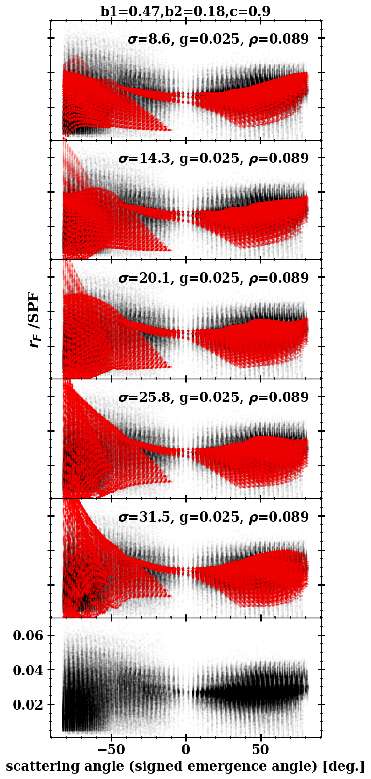
(b)  

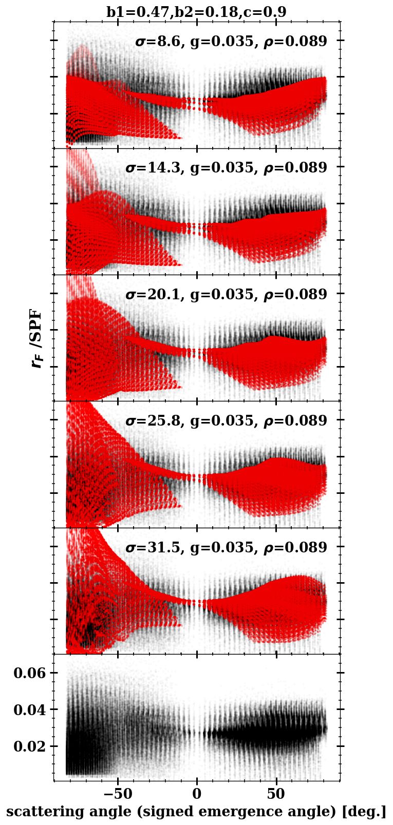
(c)  

Figure 5: Scattering profiles for the $r_{F}$ and $L_{r}$ distributions in function of the signed emergence angle. The profiles were calculated for $\sigma=\{8.6^{\circ},14.3^{\circ},20.1^{\circ},25.8^{\circ},31.5^{\circ}\}$ at three different values of specular ratio: (a) $g=1\%$, (b) $g=2.5\%$, and (c) $g=3.5\%$. $L_{r}$ distributions are in red, while $r_{F}$ distributions are in black. All panels are constrained to the same RADF and scattering angle intervals. The first-mode solution is situated between the fourth and fifth subpanels of the second column.

To evaluate the capability of the semi-numerical roughness model to describe the data variance, we devised an alternative fashion to visualize $r_{F}$ and $L_{r}$ distribution. We first remove the wider phase angle dependence by dividing the $r_{F}$ by the SPF calculated from the first-mode solution. Secondly, we split the scattering geometry space in two hemispheres: for emergence angles with associated $\varphi>90^{\circ}$, we assign a minus sign, while for those associated to $\varphi<90^{\circ}$, a positive sign is assigned. We then separate the measurements obtained at the forward-scattering configuration from those obtained at the backward-scattering configuration. Excesses and point agglomerations at either configuration can be better perceived. The results are shown in Figure 5.

The three panels in Figure 5 illustrate the roughness patterns in the RADF distribution as the roughness slope and specular factor increase. In panel 5a, where the $g$ is low, increasing roughness leads to flat forward-scattering and steeper backward-scattering as a function of the emergence angle. The agglomeration of forward-scatter faint $r_{F}$ points at high emergence angles ($\approx-50^{\circ}$) is better covered by a low $\sigma$. They are more Lommel-Seeliger scatters, which is explains the secondary MCMC modal solution at $g=1.5\%$ and $\sigma=11^{\circ}$. This secondary solution indicates that the MCMC walker recognizes that agglomeration of points is described by other parameters rather than the “global solution”. In panel 5c, the RADF is very sensitive to the increase of a few percent in the specular ratio. Higher $g$ leads to an increase in data variance and also a RADF increase in the $-40<e<0$ range. In this model, we can explain most of the high backscatter dispersion by a rough surface with a non-negligible specular contribution.

The most frequent solution is situated between the fourth and fifth subpanels ($\sigma=20.1^{\circ}$ and $25.8^{\circ}$, respectively) of column 5b. This solution covers most of the forward-scattering distribution, as well as the highest and lowest RADF points in the backscatter configuration. The modeling covers most of the data variance in the phase angle, with an average residual $\left|r_{F}-L_{r}\right|/r_{F}<0.007$.

6.1.2 Scattering phase function lobes $b_{1}$ , $b_{2}$ & $c$

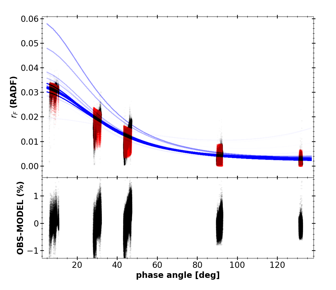
Figure 6: MapCam x-filter $r_{F}$ distribution in function of the phase angle. In the top panel, the black points represent all $r_{F}$ data under all DTMs. The superimposed red points represent the calculated $L_{r}$ distribution from the first-mode solution. The blue lines are the HG3 SPFs calculated from all $(b_{1},b_{2},c)$ 5000-step combinations. In the bottom panel, the black points are given by the difference between $\left|r_{F}-L_{r}\right|/r_{F}$, in percent.

$b_{1}$ and $c$ parameters indicate that the SPF is predominantly back-scattering ($\xi=-0.444$, as calculated by the formula in the section 4.2) in the phase angle range between of $7.5^{\circ}-130^{\circ}$. $b_{2}$ is smaller, but hints at a weak forward-scattering lobe at very large phase angle; however, more data are needed to characterize this scattering feature. The asymmetric factor may only be negative because we lack of neat detection of a secondary lobe. Negative asymmetric factors are notoriously an issue when dealing with phase function of small bodies of the solar system due to observational constrains. Other dark small bodies however have hinted into similar lack of broad forward-scattering lobes: for example, when $r_{F}$ measurements for the phase curve of the nucleus of the comet 67P/Churyumov-Gerasimenko were extended for up to $\alpha=115^{\circ}$, no signs of a second lobe was yet detected (Güttler et al., 2017).

We can also verify how well the scattering phase function describes the data. In Figure 6 we show all MCMC step SPFs calculated from MCMC steps overplotted on the $r_{F}$ distribution and the optimal $L_{r}$ distribution. Most of the SPFs calculated from steps cluster well around the most probable solution, describing the wide phase angle dependence of the $r_{F}$ distribution. The phase function does not show obvious signs of a rising second forward-scattering lobe at $\alpha=130^{\circ}$ , this feature is only hinted in the a posteriori $b_{2}$ distribution as at least ~0.2 wide. The phase function becomes flat in the $90^{\circ}-130^{\circ}$ phase angle range, where the turning point between both lobes is generally situated. Broad second lobe has been interpreted as the presence of particles in the larger-than-wavelength size regime with low internal scatterers in literature (McGuire & Hapke, 1995; Hapke, 2012). On the other hand, Zubko et al. (2015) show through discrete dipole approximation of irregular particle agglomerates that the effects of broadening forward-scattering lobe increases at $\alpha=130^{\circ}$ if the size distribution of near-wavelength-size particles becomes also becomes broader and the particles are less absorbing. This might indicate therefore the presence of small bright scatterers in the surface of Bennu in the sub-micrometer range. Nonetheless, only rigorous modeling may reveal some of the grain size properties (Mishchenko, 1994; Mishchenko & Macke, 1997; Muinonen et al., 2011; Zubko et al., 2015; Dlugach et al., 2011).

6.1.3 Approximative single-scattering albedo $\rho$

Small single-scattering albedo $\rho$ in the visible range is in-line with other B-type asteroids (Clark et al., 2010). While we lack data under $\alpha<7.5^{\circ}$ and we do not include ad hoc opposition effect terms, our estimated $\rho$ is similar to the reported geometric albedo by DellaGiustina et al. (2019). The van Ginneken et al. model takes into account the back-scattering increase as the surface gets rougher at intermediary phase angles (Figure 3), mimetizing one of the shadow-hiding attributes. Yet, Golish et al. (2020a) identify a non-linear opposition surge of ~15% rising under $\alpha<4^{\circ}$. This could possibly indicate shadow-hiding or a weak coherent-backscattering effect, which therefore hints to a slightly different value for single-scattering albedo (Mishchenko et al., 2009; Wilkman et al., 2015).

6.1.4 Specular ratio $g$

The specular reflection component is non-zero, impling a not fully diffusive surface, which is generally assumed when modeling small-body particulate surfaces. Specular reflection is proportional to the Fresnel or “mirror” reflectivity and predominant in metallic and monocrystalline materials. A specular component in the scattering process indicates that materials with such properties are possibly present on the surface. From image inspection and some previous considerations of Bennu’s composition, we suggest two potential explanations of the non-zero specular ratio: (i) Some eroding processes may lead to very flat clean-cut mineral faces on exposed boulder surfaces; or (ii) very small, bright specular inclusions could be present inside Bennu’s rock matrix.

Brightness increases associated with flat rock faces seem ubiquitous on Bennu’s surface, but they may only be an effect of orientation, as argued in Golish et al. (2020a). Their reflectances are greatly reduced after applying a photometric-topographic correction, which indicates that roughness is the main parameter controlling brightness (Section 6.3). Small bright inclusions, on the other hand, have been observed in other dark primitive small bodies, including by the contemporaneous Hayabusa2 mission in the carbonaceous chondrite-like asteroid (162173) Ryugu. Jaumann et al. (2019) have counted several in images taken by MASCOT (Mobile Asteroid Surface Scout), and they appear to be similar to those found in weakly and mildly aqueous altered carbonaceous chondrites. They can be up to three times as bright as the average Ryugu surface yet still are not spatially resolved ($\lesssim 0.5$ mm). However, the authors were not able to trace the multi-angular RADF distribution to be able to confirm the specular behavior. Bright inclusions are also observed on the ROLIS and CIVA images of Philae/Rosetta, but they are much less abundant (Schröder et al., 2017).

Potin et al. (2019) studied a recently fallen CM2 meteorite, in which both large and small grain size preparations of the meteoritic sample (called “chips” and “powder” therein) indicate the presence of a specular component in the bi-directional reflectance distribution when observed at intermediary incidence angles. The preservation of this component even after changing the grain sizes shows that the specular reflection is arising from a much smaller size scale.

As the specular elements are below the OCAMS spatial resolution, we are not able to relate the specular ratio to the size, albedo, and number, nor can we verify a relation to the bright inclusions. Images taken during reconnaissance of the sample sites may help us to further investigate the presence of specular bright inclusions.

6.1.5 Roughness RMS slope $\sigma$

The roughness RMS slope $\sigma$ is the parameter controlling the major part of the RADF multi-angular spread in the van Ginneken et al. (1998) model. The $\sigma$ value of $27_{-5}^{\circ+1}$ is very similar to the v-band average roughness slopes $\bar{\theta}$ of other disk-resolved asteroids derived using Hapke shadowing-roughness model (Hapke, 1984). The asteroids Gaspra (S-type, Helfenstein et al., 1994), Eros (Sw-type, Li et al., 2004), Steins (Xe-type, Spjuth et al., 2012), Ryugu (Cb-type, Tatsumi et al., in prep.), and the cometary nucleus of 67P/C-G (Hasselmann et al., 2017), all have $\bar{\theta}$ situated near $28^{\circ}$. These objects have different sizes, ages, and compositions, but the same optical roughness slopes may indicate a similar size scale for their irregularities. Micro-erosions in the space environment — i.e., processes such as micro-cratering, particle agglutination, and regolith friction — possibly quickly converge to surface micro-irregularities on the order of $25^{\circ}-30^{\circ}$.

The optical roughness is smaller than the roughness obtained through thermal infrared modeling ($43\pm 1^{\circ}$, DellaGiustina et al., 2019). The “thermal roughness” is most sensitive to the smaller end of the spatial scale, i.e., ~2 cm. This indicates a break in surface fractality between the optical, acting on the order of ~0.1-1 mm (Cord et al., 2003), and thermal centimeter scales. A surface cannot sustain infinite fractality, and the break could suggest a regime interface from topographic to particle size irregularities. This is different from what has been observed on the Moon. Helfenstein & Shepard (1999) have shown, by analysing spatially resolved Apollo mission images, that lunar soil is consistently fractal through a decreasing size scale. Lunar regolith, however, is dominated by particles of a few tens of microns in size, which may help sustain the fractality for even smaller size scales, while Bennu shows weak indication of such structure sizes. If fractal roughness can be used as an indication of micrometric particles, we may have another discriminant tool to constrain their presence.

6.2 Spectro-photometry of the sample site DTM zones

Figure 7: The spectral behavior of the surface scattering parameters and the scattering phase function in the four OCAMS bands. The blue dots represent the mode solution from their a posteriori distributions, while the errorbars represent the midspread. In the top left panel (parameter $\rho$) the average Bennu OVIRS EQ3 spectrum segment ($\lambda=$450 – 950 nm and $\alpha=7.5^{\circ}$– $8.0^{\circ}$) has been rescaled to match the v-filter albedo (factor of $\times 2.17$) and is superimposed in grey. A segment jump around 660 nm, i.e., where the spectrum goes from one filter to the next, was removed for clarity. For the scattering phase functions, the bottom center and bottom right panels show the zoom-in at small and large phase angles.

We investigated the spectral behavior of the approximate single-scattering albedo and other parameters using the same inversion technique described in Section 5. For all of the OCAMS multi-band RADF data except those from the x-filter (Section 6.1), we performed an MCMC evaluation dispatching a chain of 2000 steps. The mode of the distributions, as well as its midspread for each parameter as a function of the wavelength, is shown in the Figure 7. Heavily skewed error bars indicate the presence of a secondary mode in the a posteriori distribution. Overall, the surface properties show a weak spectral trend except in albedo $\rho$ and the asymmetric factor $\xi$.

The albedo $\rho$ presents the expected negative spectral slope ($\varsigma=-0.53\pm 0.08\%/\mu m$) related to Bennu’s B spectral asteroid type (Lauretta et al., 2019), and agrees well with the OVIRS EQ3 global spectral segment in the visible range taken at $\alpha=7.5^{\circ}$. OVIRS spectra have been radiometrically calibrated by Simon et al. (2018). We report an albedo $\rho_{v^{\prime}}$ of $4.64_{-0.09}^{+0.08}\%$ at 550 nm. The asymmetric factor $\xi$ shows that Bennu becomes more backscattered as wavelength increases, following same spectral albedo behavior. Trends where $\xi$ is coupled with $\rho$ have been seen on the surfaces of other dark atmosphereless bodies, such as Ceres (Li et al., 2019) and the nucleus of 67P/C-G (Fornasier et al., 2015), both observed in the visible range. In the case of Bennu, the $\xi$ is controlled by the influence of a second lobe beyond $\alpha>130^{\circ}$, as shown in the bottom right panel of Figure 7. The second lobe weakens and the phase function becomes more back-scattered as wavelength increases.

All of the other surface parameters point to scattering characteristics already probed through the inversion of the x-filter data in Section 6.1. The parameters $c$, $b_{1}$ and $b_{2}$ indicate a backscattering surface with two modal solutions for asymmetric factor ($\xi^{(1)}=-0.360\pm 0.030$ and $\xi^{(2)}=-0.444\pm 0.020$), and a possible presence of a weak forward-scattering lobe. The roughness RMS $\sigma$ ranges between $20^{\circ}$ and $27^{\circ}$ overall and the specular ratio $g$ seems largely invariant in the visible range.

Figure 8: The approx. single-scattering albedo $\rho$ spectro-photometry (blue symbols), in percentage, alongside the OVIRS EQ3 spectral segment in the visible range (in grey) for the high-precision DTM zones containing the four sample site candidates. In each panel, the spectro-photometry of the DTM zones are reproduced repeatedly in red, for better comparison. The OVIRS were rescaled to match the $\rho_{v^{\prime}}$at 550 nm. A segment jump around 660 nm was removed for clarity. The y-axis and x-axis are fixed to same interval for clarity. Factors & Symbols: Nightingale (—, solid line) — $\times 2.23\%$; Osprey ($--$, dashed line) — $\times 2.32\%$; Kingfisher ($-\cdot$, dashed-dotted line) — $\times 2.23\%$; Sandpiper ($\cdot\cdot\cdot$, dotted line) — $\times 2.15\%$.

We have also investigated the spectro-photometry of the albedo $\rho$ for each of the four DTM zones containing the sample site candidates. To obtain their albedo $\rho$, we traced and binned each of their $r_{F}(\lambda)$ phase curves in the same fashion as described in the Section 5. We normalized the multi-band phase curves by dividing them by $L_{r}(\lambda)$ calculated from the optimal first-mode parameters shown in Figure 7, leaving only the parameter $\rho$ free. Their approximative single-scattering albedo spectra are shown in Figure 8 alongside their average OVIRS EQ3 spectrum. The site spectra were averaged for all acquisitions superimposing more than half the nominal area of the sites. There, as well, we find good agreement between the $\rho$ spectral trend and the OVIRS EQ3 spectra for the four sample site DTM zones. Nightingale, which was ultimately chosen as the primary sample collection site for OSIRIS-REx, is the darkest and least blue among the four, with $\rho_{v^{\prime}}^{(N)}=4.5\pm 0.06\%$ and spectral slope of $\varsigma^{(N)}=-0.51\pm 0.16\%/\mu m$. For the other candidate sites, we obtain: Osprey, $\rho_{v^{\prime}}^{(O)}=4.9\pm 0.04\%$ and $\varsigma^{(O)}=-0.72\pm 0.25\%/\mu m$; Kingfisher, $\rho_{v^{\prime}}^{(K)}=4.84\pm 0.04\%$ and $\varsigma^{(K)}=-0.69\pm 0.07\%/\mu m$; and Sandpiper, $\rho_{v^{\prime}}^{(S)}=4.64\pm 0.05\%$ and $\varsigma^{(S)}=-0.70\pm 0.27\%/\mu m$.

6.3 Photometric correction and the role of roughness

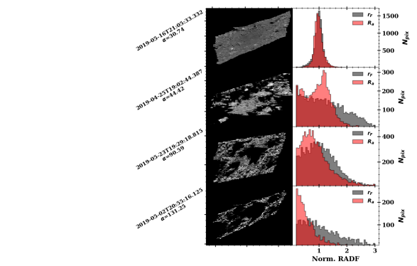
(a)(b)

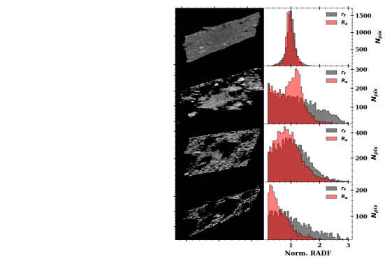
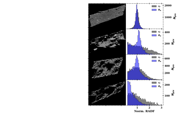
(c)(d)

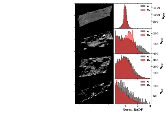
Figure 9: Photometric correction of Nightingale images using mixed solutions. The correction was applied to four images taken at different phase angles and other observational conditions. Their timestamps and corresponding phase angles are listed in the beginning of each row. Each panel corresponds to a different roughness solution: (a) $\sigma=27^{\circ}$; (b) $\sigma=10^{\circ}$; (c) a mixture of both solutions; and (d) Lommel-Seeliger correction, for reference. The first columns of each panel show the corrected images. Image contrasts and brightness are fixed to same maximum and minimum levels in all three panels. In the third column of each panel, the normalized $r_{F}$ histograms of pixels in grey, and the $R_{a}$ histograms representing the photometrically corrected RADF ratio are shown in red.

We checked the capacity of the roughness model to photometrically correct spatially resolved images of a small body surface. For our tests, we chose four images of the Nightingale site taken at intermediary to high phase angles. We verified three kinds of solutions of roughness RMS slope: (a) $\sigma=27^{\circ}$, the first-mode solution; (b) $\sigma=11^{\circ}$, second-mode solution; and (c) a mixture of both solutions. All the other parameters were fixed at the first-mode solution of Section 6.1.

We decided to also undertake tests with a lower $\sigma$ motivated by the second mode in the a posteriori distribution (Figure 4). This trend is also evident in Figure 5, where part of the agglomeration of forward-scatter faint $r_{F}$ points at high emergence angles are better covered by a low $\sigma$. In the case of mixing the two solutions, solution (a) or solution (b) was assigned to a given facet depending on the smallest $\chi^{2}=\sum\left(r_{F}-L_{r}^{(a,b)}\right)^{2}$ residual between the $L_{r}$ from one of two solutions and pixel $r_{F}$ assigned to the same facet. The facet RADF is divided by the $L_{r}$ calculated from the appropriate observational condition using the optimal first-mode solution. In the final step, the shadowed facets, those ray-traced from the shape model, are removed, and the corrected RADF ratio $R_{a}$ for every pixel is estimated as described in Appendix A.

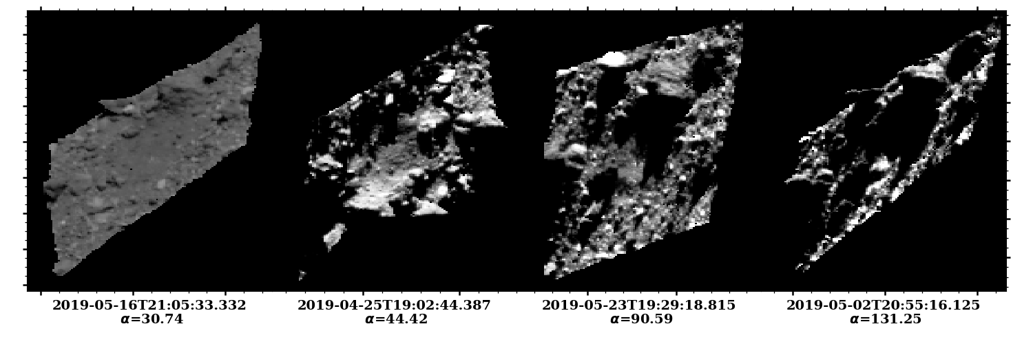
Figure 10: Four EQ image segments of Nightingale in different phase angles. The contrast and brightness are all scaled to the same levels as in the Figure 9.

We show in Figure 9 the results of those verifications in four intermediary to large phase angles. For cross-checking, the original image segments of Nightingale, in the same four different phase angles, are shown in the Figure 10. A qualitatively good photometric correction is reached when the central tendency of the corrected RADF $R_{a}$ distribution is unity. This means that only intrinsic reflectance variation remains in the data. In Figure 9ab, both low and intermediary roughness slopes yield very similar photometric corrections for intermediary phase angles ($\alpha\simeq 30^{\circ}$ and $\alpha\simeq 45^{\circ}$). In this range, surface roughness is not the main optical factor controlling reflectance variance, and a Lommel-Seeliger correction is enough to yield sufficient results. For $\alpha\simeq 90^{\circ}$ and $\alpha\simeq 130^{\circ}$, however, the fixed-roughness solutions are insufficient to remove the photometric-topographic brightness trend, or they overcorrect it, as in the case of solution (a). This dichotomy between intermediary and high phase angles is very revealing when we look to the mixed solutions of Figure 9c. By mixing intermediary and low roughness slopes we obtain a visible improvement in the correction from $30^{\circ}$ to $90^{\circ}$ phase angle. The apparent bright topographic structures have their RADF reduced by a factor of up to 3 times at $\alpha\simeq 30^{\circ}$ and $\alpha\simeq 90^{\circ}$, indicating that these “speckles” are not responsible for the specular component. For all tested images, the “replacement ratio”, i.e., the ratio of facets with solution (a) to total number of facets, is about $50\pm 5\%$. This “replacement” shows no preferential facet at certain incidence, azimuth, or emergence angles for all Nightingale images. It means that, at the sub-pixel scale, Bennu’s surface shares two main diffusive components, and only when both components are taken into account is the photometric correction improved.

(a)

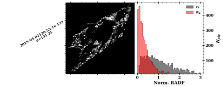
(b)

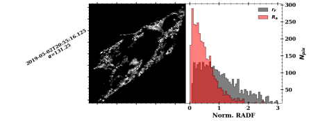
(c)

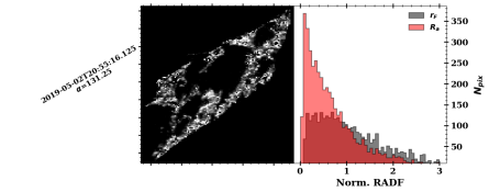
Figure 11: Photometric correction of EQ2 UT 2019-05-02T20:55:16.125 image of Nightingale taken at $\alpha\simeq 130^{\circ}$. (a) Corrected image using $\sigma=55^{\circ}$; (b) same as (a) using $\sigma=0^{\circ}$; (c) same as (b) without macro-shadow sub-pixel removal. All images are constrained to same contrast and brightness levels.

For images taken at $\alpha\simeq 130^{\circ}$, the photometric correction at the sub-pixel level becomes more difficult to tackle. The images have an average $r_{F}$ of 0.093% with standard deviation in a comparable value of 0.1%, it shows that the reflectance is more sensitive to topographic features, and therefore, to the shape model limitations. The mixed solution (Figure 9c) still grants a RADF that is about two to three times as bright as the data, which indicates that there is another component reducing even further the RADF at high phase angles. To tackle this, we corrected the images using $\sigma=55^{\circ}$ and $\sigma=0^{\circ}$, the upper and lower validity limit of the model, to check how the $L_{r}$ distribution behaves. We also added a third verification, where macro-shadows are not discounted from the pixel RADF calculation. The effects of macro-shadows may indicate whether topographic features are playing a role in the RADF distribution. We present the three verifications in Figure 11. We can first observe that neither high or very low roughness slope produce enough faint $L_{r}$ values to correct the data. Figure 11c, when compared to 11b, shows that a considerable number of pixels become fainter if the macro-shadows are not discounted, which leads the $R_{a}$ distribution to get more skewed to faint levels. This indicates that, for a high phase angle, a shape model that better accounts for sub-pixel meso-scale topography is as important as the sub-millimeter roughness.

As the slope distribution of boulder and other topographic features can be highly non-Gaussian (Labarre et al., 2017), we propose that mathematically extending the van Ginneken et al. (1998) model formulation to non-Gaussian slope distributions might in part account for the faintness at higher phase angles (Brown, 1980; Bahar & Fitzwater, 1983). Another suggestion is to account for fractality (Shkuratov et al., 2003) in the diffusive reflection. In this case, the faintness would come from setting the appropriate fundamental scattering law on the fractal elements. This could be done using the Akimov disk law (Akimov, 1976, 1979) as fundamental scattering law or, more extensively, directly computing the infinite series from Shkuratov et al. (2018), a model that proposes to describe rough surfaces through multi-scale Gaussian ondulations. The latter solution may implicate in further computing time and also departing from the simplicity proposed by the application of van Ginneken et al. framework.

7 Discussion and Conclusion

We have reintroduced the van Ginneken et al. (1998) semi-numerical model to treat first-order light scattering arising from rough, optically thick surfaces, now coupled with DTM shadow ray-tracing to account for meso-scale “rocky” topography. Our scientific goal is to provide a parametric description of Bennu’s surface to support laboratory preparations of surface analogs and the spectral and imaging interpretation of OSIRIS-REx data. We obtained the scattering parameters and RMS roughness slope of the dark asteroid Bennu by solving the inversion problem using the MCMC technique applied to MapCam four-band RADF data for OSIRIS-REx’s top four candidate sample sites together. We also made use of the high-resolution OLA DTMs produced for these areas of Bennu’s surface.

The MCMC technique yields a posteriori distributions for each parameter, revealing interesting aspects of Bennu’s surface: while the RMS roughness slope of $27_{-5}^{\circ+1}$ is in line with what has been obtained for other asteroids using the Hapke shadowing function, we are puzzled by the indication of a non-zero specular reflection ratio from the surface ($2.6_{-0.8}^{+0.1}\%$). The specular reflection hints at inclusions, possibly of monocrystalline origin, contributing to the surface reflectance in a way that is generally not taken into account by fully diffusive approximative radiative transfer models (Hapke, 2012). It may be a direct expression of a compositional sub-centimetric component on the surface. A plausible candidate for the specular reflection contribution is carbonate crystal inclusions. Carbonates have been detected by OVIRS in several areas of Bennu, including in the surrounding Nightingale (Kaplan et al., 2020, in press). Calcites and dolomites appear to be the most abundant component. In some zones imaged by PolyCam, the carbonates inclusions appear to be present as bright spots and bright veins of tens of centimeter size on surface of boulders, whereas the vast majority does not display any obvious sign of their presence, possibly due to the imaging spatial resolution. This likely indicates that most of the carbonate is sub-centimetric. The presence of carbonates, as well as their possible crystalline phase, provides constraints on the thermal and hydration history of Bennu and the composition of its parent body (Kaplan et al., 2020, in press).

As for the diffuse rough component, the meso-scale “rocky” topography contribution is expected to be pre-modeled through DTM ray-tracing, leaving the micro-scale roughness (Shkuratov et al., 2005) to be described by the van Ginneken et al. (1998) model. However, the analysis of the photometric correction of OCAMS images taken at varied phase angles indicates a more complex scenario. Up to $\alpha\simeq 90^{\circ}$, the photometric correction is greatly improved by mixing two different solutions for roughness (one with low RMS $\sigma$ and another with global RMS $\sigma$), a bi-modality already perceived from the MCMC a posteriori distributions. This bi-modality may indicate the presence of widespread low-roughness rock faces with quasi-Lommel-Seeliger scattering immersed into other irregularities account for the broader global distribution of larger roughness. This kind of landscape is apparently revealed by higher spatially resolved images taken of the candidate sample sites (Golish et al., 2020a). We have shown that most of Bennu’s brightness variation can be explained by tuning the roughness slope distribution.

Neither the mixing nor pushing the model to its limits are not enough to yield a satisfactory photometric correction for images obtained at $\alpha\simeq 130^{\circ}$. This points to two main possible effects: (i) the Lommel-Seeliger scattering law does not reflect the fundamental diffusive scattering behavior from Bennu’s surface as we approach higher phase angles, which is known to be a poor law for planetary surfaces (Shkuratov et al., 2011, 2018). (ii) Bennu’s tilt distribution is not Gaussian-like at a spatial scale smaller than the DTM facet size; an over-abundance of small or high slopes may account for part of the needed faintness. As for the former, the van Ginneken et al. model can be mathematically adapted to accomodate any scattering law, which is a relevant feature for future applications, and may reveal which is the actual proper fundamental scattering law to be used when considering the smallest unitary tilts in planetary rough surface distributions. As for the latter, the shadowing can be replicated when further high-resolution DTMs are available for the candidate sample sites and all of Bennu’s surface. Nonetheless, in future applications of the semi-numerical model, it may be worthwhile to expand $P_{a}(\theta_{a})$ to non-Gaussian slope distributions, which may lead to a solution that tackles the probabilistic terms $P_{ill+vis}$ and $L_{rd}^{(2)}$ through their full integration (Brown, 1980; Bahar & Fitzwater, 1983; Oren & Nayar, 1995; Bourlier et al., 2002).

We report a backscatter scattering phase function for the phase angle range between $7.5^{\circ}$ and $130^{\circ}$, without any expressive spectral trend in the visible range. The MCMC inversion hints at a possible second forward-scatter lobe of at least ~0.2 width. This leads to two possible solutions for the asymmetric factor ($\xi^{(1)}=-0.360\pm 0.030$ and $\xi^{(2)}=-0.444\pm 0.020$). We also report a dark global approximate single-scattering albedo at 550 nm from the collective analysis of all candidate sample sites of $4.64_{-0.09}^{+0.08}\%$ . The single-scattering albedo from the MapCam four-band colors has a similar spectral trend to the global average OVIRS EQ3 spectrum; the four sites together provide a general description of Bennu’s colors. We also find very good agreement in the spectral slopes between the single-scattering spectro-photometry and the OVIRS EQ3 spectra of each site candidate separately.

On 13 December 2019, Nightingale was announced as the primary sample site. Although we have not yet conducted a dedicated photometric analysis of this site, we can provide some predictions on the surface material structure based on the average photometric parameters and Nightingale’s albedo. Our evidence supports a lack of widespread sub-micrometric dust, given that the RADF distribution is sufficiently explained by single-scattering processes. The formation of shadows by macroscopic roughness in the visible range indicates that the roughness size scale is much larger than the wavelength, above thousands of microns to few millimeters, if the break in fractality according to the thermal roughness-scale is real. The specular component may indicate that carbonates are widespread and will likely be present in the collected sample. Nightingale’s low albedo, on the other hand, could suggest fewer rock faces larger than OCAMS pixel-size scattering back to the observer, thus decreasing photometric variability. Therefore, Nightingale’s roughness size scale may be much smaller than Bennu’s average.

Acknowledgements. P. H. H. thanks Dr. Alice Bernard for her support. This work was funded by the DIM-ACAV+ project (ï¿œle-de-France, France) and is based upon work supported by NASA under Contract NNM10AA11C issued through the New Frontiers Program. The authors thank all teams and people that helped in the accomplishment of the OSIRIS-REx mission. P. H. H. thanks all people concerned in developing and keeping the Cython language, and Numpy and Scipy libraries for Python. OLA and funding for the Canadian authors were provided by the Canadian Space Agency. Images and kernels will be available via the Planetary Data System (PDS) (https://sbn.psi.edu/pds/resource/orex/). Data are delivered to the PDS according to the OSIRIS-REx Data Management Plan available in the OSIRIS-REx PDS archive. DTMs will be available in the PDS 1 year after departure from the asteroid.

References

Appendix A

As we are dealing with unresolved shadowed surfaces that are getting expressed into a detector by a single pixel intensity $I_{\lambda}(i,e,\alpha,\varphi)$, the pixel intensity can get split into two terms (the meanings of all variables are listed in the Table 2):

$$I_{\lambda}(i,e,\alpha,\varphi)\varOmega_{T}=\sum_{j}\mu_{0}R_{a}^{(j)}(\alpha)D_{a}^{(j)}(i,e,\varphi)\varOmega_{e}^{(j)}S_{\lambda}+$$

$$+\sum_{j}I_{n}\left(1-\varOmega_{e}^{(j)}\right)$$ (14)

In the equation above we follow the assumption that the reflected intensity can be decomposed in two functions: a scattering phase function $R_{a}^{(j)}(\alpha)$ and photometric-topographic “disk function” $D_{a}^{(j)}(i,e,\varphi)$ (Shkuratov et al., 2011). The first term represents the total intensity contribution of all visible and illuminated facet area covered by the pixel (Wilkman et al., 2015). The second term is the second-order scattered intensity contribution of all of the surface not directly illuminated but yet visible. This quantity is approximated to a diffusive reflectance (Hapke, 2012) by assuming that the surrounding illuminated surfaces can be treated as an isotropic light source (reflected light from all surrounding illuminated topography). By considering that all facet reflectances $R_{a}(\alpha)$ are albedo-homogeneous, and that every $r_{0}$ is isotropic and homogeneous, we can obtain the phase function reflectance $R_{a}(\alpha)$ per pixel by re-arranging:

$$R_{a}(\alpha)=\left[\frac{I_{\lambda}(i,e,\alpha,\varphi)}{S_{\lambda}}-r_{0}\left(1-\sum_{j}\varOmega_{e}^{(j)}\right)\right]\times$$

$$\times\sum_{j}\frac{\varOmega_{T}}{D_{a}^{(j)}(i,e,\varphi)\mu_{0}\varOmega_{e}^{(j)}}$$ (15)

Table 2: Variable in equations of Appendix A.

Variable	Description
$j$	facet index
$I_{\lambda}$	Pixel Intensity
$I_{n}$	retro-scattered intensity from shadowed surface
$R_{a}$	phase function reflectance or the corrected radiance factor ratio
$D_{a}$	“disk function” ratio
$\varOmega_{T}$	Pixel solid angle
$\varOmega_{e}$	Fraction of Solid angle of a surface element
$\mu_{0}$	cosine of incidence angle
$S_{\lambda}$	Solar irradiance
$r_{0}$	diffusive reflectance

Operations to remove the photometric-topographic effect, the so-called “disk function”, and the contribution of shadows were calculated using the equation above. In our paper the $\mu_{0}D_{a}^{(j)}(i,e,\varphi)$ joint term is replaced by $L_{r}(i,e,\alpha,\varphi)$ calculated from the semi-numerical roughness model (Section 4), therefore $R_{a}(\alpha)\longrightarrow R_{a}$, the corrected RADF ratio. This operation reduces the dependence of the radiance to any large-scale shadow that the DTM is capable of tracing, leaving out only the intrinsic dependence on sub-facet roughness and scattering.

The diffusive reflectance is somewhat related to the second-order scattering albedo. During our image treatment, instead of leaving it as another free parameter, we set $r_{0}$ very small (=1e-5); therefore, macro-shadows will have a minimal contribution to the pixel RADF. The only error that we may incur is to overestimate the RADF for some heavily shadowed pixels.

References

- Acton et al. (2018) Acton, C., Bachman, N., Semenov, B., & Wright, E. 2018, planss, 150, 9
- Acton (1996) Acton, C. H. 1996, planss, 44, 65
- Akimov (1976) Akimov, L. A. 1976, Soviet Astronomy, 19, 385388
- Akimov (1979) —. 1979, Soviet Astronomy, 23, 231
- Bahar & Fitzwater (1983) Bahar, E., & Fitzwater, M. A. 1983, Radio Science, 18, 566
- Barnouin et al. (2020) Barnouin, O. S., Daly, M. G., Palmer, E. E., et al. 2020, planss, 180, 104764
- Behnel et al. (2011) Behnel, S., Bradshaw, R., Citro, C., et al. 2011, Computing in Science and Engineering, 13, 31
- Bourlier et al. (2002) Bourlier, C., Berginc, G., & Saillard, J. 2002, IEEE Transactions on Antennas and Propagation, 50, 312
- Brown (1980) Brown, G. S. 1980, IEEE Transactions on Antennas and Propagation, 28, 788
- Clark et al. (2010) Clark, B. E., Ziffer, J., Nesvorny, D., et al. 2010, Journal of Geophysical Research (Planets), 115, E06005
- Cord et al. (2003) Cord, A. M., Pinet, P. C., Daydou, Y., & Chevrel, S. D. 2003, Icarus, 165, 414
- Cuzzi et al. (2017) Cuzzi, J. N., Chambers, L. B., & Hendrix, A. R. 2017, Icarus, 289, 281
- Daly et al. (2017) Daly, M. G., Barnouin, O. S., Dickinson, C., et al. 2017, Space Science Reviews, 212, 899
- Davidsson et al. (2015) Davidsson, B. J. R., Rickman, H., Band field, J. L., et al. 2015, Icarus, 252, 1
- DellaGiustina et al. (2019) DellaGiustina, D. N., Emery, J. P., Golish, D. R., et al. 2019, Nature Astronomy, 3, 341
- Dlugach et al. (2011) Dlugach, J. M., Mishchenko, M. I., Liu, L., & Mackowski, D. W. 2011, Journal of Quantitative Spectroscopy and Radiative Transfer, 112, 2068 , polarimetric Detection, Characterization, and Remote Sensing
- Fairbairn (2005) Fairbairn, M. B. 2005, JRASC, 99, 92
- Feller et al. (2016) Feller, C., Fornasier, S., Hasselmann, P. H., et al. 2016, Monthly Notes of Royal Astronomical Society, 462, S287
- Fornasier et al. (2015) Fornasier, S., Hasselmann, P. H., Barucci, M. A., et al. 2015, Astronomy and Astrophysics, 583, A30
- Goguen et al. (2010) Goguen, J. D., Stone, T. C., Kieffer, H. H., & Buratti, B. J. 2010, Icarus, 208, 548
- Golish et al. (2020a) Golish, D., DellaGiustina, D., Li, J.-Y., et al. 2020a, Icarus, 113724
- Golish et al. (2020b) Golish, D. R., Drouet d’Aubigny, C., Rizk, B., et al. 2020b, Space Science Reviews, 216, 12
- Güttler et al. (2017) Güttler, C., Hasselmann, P. H., Li, Y., et al. 2017, Monthly Notes of Royal Astronomical Society, 469, S312
- Haario et al. (2001) Haario, H., Saksman, E., & Tamminen, J. 2001, Bernoulli, 7, 223
- Hamilton et al. (2019) Hamilton, V. E., Simon, A. A., Christensen, P. R., et al. 2019, Nature Astronomy, 3, 332
- Hapke (1984) Hapke, B. 1984, Icarus, 59, 41
- Hapke (2012) —. 2012, Theory of Reflectance and Emittance Spectroscopy, 2nd edn. (Cambridge University Press)
- Hapke (2013) —. 2013, JQSRT, 116, 184
- Hartley & Zisserman (2004) Hartley, R. I., & Zisserman, A. 2004, Multiple View Geometry in Computer Vision, 2nd edn. (Cambridge University Press, ISBN: 0521540518)
- Hasselmann et al. (2016) Hasselmann, P. H., Barucci, M. A., Fornasier, S., et al. 2016, Icarus, 267, 135
- Hasselmann et al. (2017) —. 2017, Monthly Notes of Royal Astronomical Society, 469, S550
- Hasselmann et al. (2019) Hasselmann, P. H., Fornasier, S., Barucci, M. A., et al. 2019, in EPSC-DPS Joint Meeting 2019, Vol. 2019, 225
- Helfenstein & Shepard (1999) Helfenstein, P., & Shepard, M. K. 1999, Icarus, 141, 107
- Helfenstein et al. (1994) Helfenstein, P., Veverka, J., Thomas, P. C., et al. 1994, Icarus, 107, 37
- Irvine (1965) Irvine, W. M. 1965, Astrophysical Journal, 142, 1563
- Ito et al. (2018) Ito, G., Mishchenko, M. I., & Glotch, T. D. 2018, Journal of Geophysical Research (Planets), 123, 1203
- Jaumann et al. (2019) Jaumann, R., Schmitz, N., Ho, T. M., et al. 2019, Science, 365, 817
- Kaplan et al. (2020) Kaplan, H. H., Lauretta, D. S., Simon, A. A., et al. 2020, Science
- Labarre et al. (2017) Labarre, S., Ferrari, C., & Jacquemoud, S. 2017, Icarus, 290, 63
- Lauretta et al. (2017) Lauretta, D. S., Balram-Knutson, S. S., Beshore, E., et al. 2017, Space Science Reviews, 212, 925
- Lauretta et al. (2019) Lauretta, D. S., DellaGiustina, D. N., Bennett, C. A., et al. 2019, Nature, 568, 55
- Li et al. (2004) Li, J., A’Hearn, M. F., & McFadden, L. A. 2004, Icarus, 172, 415
- Li et al. (2015) Li, J.-Y., Helfenstein, P., Buratti, B., Takir, D., & Clark, B. E. 2015, Asteroid Photometry (University of Arizona press), 129–150
- Li et al. (2019) Li, J.-Y., Schroeder, S. E., Mottola, S., et al. 2019, Icarus, 322, 144
- Markkanen et al. (2018) Markkanen, J., Agarwal, J., Väisänen, T., Penttilä, A., & Muinonen, K. 2018, Astrophysical Journal Letter, 868, L16
- McGuire & Hapke (1995) McGuire, A. F., & Hapke, B. W. 1995, Icarus, 113, 134
- Minnaert (1941) Minnaert, M. 1941, Astrophysical Journal, 93, 403
- Mishchenko (1994) Mishchenko, M. I. 1994, JQSRT, 52, 95
- Mishchenko (2009) —. 2009, Journal of Quantitative Spectroscopy & Radiative Transfer, 110, 808
- Mishchenko et al. (2009) Mishchenko, M. I., Dlugach, J. M., Liu, L., et al. 2009, Astrophysical Journal, 705, L118
- Mishchenko & Macke (1997) Mishchenko, M. I., & Macke, A. 1997, JQSRT, 57, 767
- Mosegaard & Tarantola (1995) Mosegaard, K., & Tarantola, A. 1995, Journal of Geophysical Research, 100, 12,431
- Muinonen et al. (2011) Muinonen, K., Parviainen, H., Näränen, J., et al. 2011, Astronomy and Astrophysics, 531, A150
- Nayar (1991) Nayar, S. K. 1991, PhD thesis, CARNEGIE-MELLON UNIVERSIT
- Oren & Nayar (1995) Oren, M., & Nayar, S. K. 1995, International Journal of Computer Vision, 14, 227
- Potin et al. (2019) Potin, S., Beck, P., Schmitt, B., & Moynier, F. 2019, Icarus, 333, 415
- Rizk et al. (2018) Rizk, B., Drouet d’Aubigny, C., Golish, D., et al. 2018, Space Science Reviews, 214, 26
- Scheeres et al. (2019) Scheeres, D. J., McMahon, J. W., French, A. S., et al. 2019, Nature Astronomy, 3, 352
- Schmidt & Fernando (2015) Schmidt, F., & Fernando, J. 2015, Icarus, 260, 73
- Schröder et al. (2017) Schröder, S. E., Mottola, S., Arnold, G., et al. 2017, Icarus, 285, 263
- Scott (1992) Scott, D. W. 1992, Multivariate Density Estimation: Theory, Practice and Visualization. (John Wiley & Sons, Inc.), doi:10.1002/9780470316849
- Shkuratov et al. (2011) Shkuratov, Y., Kaydash, V., Korokhin, V., et al. 2011, planss, 59, 1326
- Shkuratov et al. (2012) —. 2012, Journal of Quantitative Spectroscopy and Radiative Transfer, 113, 2431
- Shkuratov et al. (2004) Shkuratov, Y., Ovcharenko, A., Zubko, E., et al. 2004, jqsrt, 88, 267
- Shkuratov et al. (2003) Shkuratov, Y., Petrov, D., & Videen, G. 2003, Journal of the Optical Society of America A, 20, 2081
- Shkuratov et al. (2018) Shkuratov, Y., Korokhin, V., Shevchenko, V., et al. 2018, Icarus, 302, 213
- Shkuratov et al. (2005) Shkuratov, Y. G., Stankevich, D. G., Petrov, D. V., et al. 2005, Icarus, 173, 3
- Silverman (1986) Silverman, B. W. 1986, Density Estimation for Statistics and Data Analysis, Chapman & Hall/CRC Monographs on Statistics & Applied Probability (Taylor and Francis)
- Simon et al. (2018) Simon, A., Reuter, D., Gorius, N., et al. 2018, Remote Sensing, 10, 1486
- Smith (1967) Smith, B. 1967, IEEE Transactions on Antennas and Propagation, 15, 668
- Spjuth et al. (2012) Spjuth, S., Jorda, L., Lamy, P. L., Keller, H. U., & Li, J.-Y. 2012, Icarus, 221, 1101
- Van Der Walt et al. (2011) Van Der Walt, S., Colbert, S. C., & Varoquaux, G. 2011, Computing in Science & Engineering, 13, 22
- van Ginneken et al. (1998) van Ginneken, B., Stavridi, M., & Koenderink, J. J. 1998, Applied Optics, 37, 130
- Wilkman et al. (2015) Wilkman, O., Muinonen, K., & Peltoniemi, J. 2015, planss, 118, 250
- Zubko et al. (2015) Zubko, E., Shkuratov, Y., & Videen, G. 2015, jqsrt, 150, 42
- Zubko et al. (2001) Zubko, E. S., Shkuratov, Y. G., & Muinonen, K. 2001, Optics and Spectroscopy, 91, 273