Gravitational lens time-delay as a probe of a possible time variation of the fine-structure constant

Abstract

A new method based on large scale structure observations is proposed to probe a possible temporal variation of the fine-structure constant ($\alpha$). Our analyses are based on time-delay of Strong Gravitational Lensing and Type Ia Supernovae observations. By considering the runaway dilaton scenario, where the cosmological temporal evolution of the fine-structure constant is given by $\frac{\Delta\alpha}{\alpha}\approx-\gamma\ln{(1+z)}$, we obtain limits on the physical properties parameter of the model ($\gamma$) at the level $10^{-2}$ ($1\sigma$). Although our limits are less restrictive than those obtained by quasar spectroscopy, the approach presented here provides new bounds on the possibility of $\frac{\Delta\alpha}{\alpha}\neq 0$ at a different range of redshifts.

I Introduction

It is well-known that the standard physics is characterized by a set of laws and fundamental couplings which were historically assumed to be space-time invariant. One of the first contributors to ask about this conjecture was Dirac (1934) Dirac:1938mt , arguing that fundamental couplings might not be pure numbers that occur in many theories, but they might depend on the state of the Universe. Thereafter, many theoretical and observational approaches have come searching for a space-time variation of the fundamental couplings of nature (see a detailed review in Uzan:2010pm ; Martins:2017yxk ). Although the search for a possible varying fundamental couplings has raised the interest of many cosmologists, the general relativity theory prohibits any violation since it would violate the Equivalence Principle Ray:2019lxv .

In most extensions of the current standard cosmological model, the fundamental couplings are expected to vary leading to consequences that need to be probed with observational data Bekenstein256 ; SBM ; BL ; BG ; MWMK ; BBCMAA ; Chodos ; wuwang ; Kiritsis . In the astronomical context, particularly from white dwarfs astronomical observations, constraints on $\Delta\alpha/\alpha$ at the level $(2.7\pm 9.1)\times 10^{-5}$ were obtained by using gravitational potential Landau:2020vkr ; Bainbridge:2017lsj , where $\alpha$ is the fine structure constant. More recently, 4 new spectral observations of very high redshift quasars, up to $z\approx 7.1$, have shown no evidence for a temporal variation of the fine-structure constant (by the so-called many-multiplet method) Wilczynska . However, when the authors combined those measurements with a large existing sample at lower redshifts, it was pointed out that a spatial variation of $\alpha$ is preferred over a no-variation model at the $3.7\sigma$ level (see other discussions about $\alpha$ spatial variation in webb1999 ; Ubachs:2017zmg ). However, very recently, the authors of the Ref. Lee:2021kjr showed that fitting turbulent models in quasars necessarily generates or enhances model non-uniqueness, adding a substantial additional random uncertainty to $\Delta\alpha/\alpha$. In other words, there is a degeneracy between the absorption structure and turbulent models, each giving different $\Delta\alpha/\alpha$ values.

By using the physics of cosmic microwave background radiation (CMB), the Ref. Hart:2019dxi presented updated constraints on the variation of the fine-structure constant and the effective electron rest mass $m_{e}$ during the cosmological recombination era. The authors showed that $\alpha$ and $m_{e}$ can straightly modify the recombination history at $z\approx 1100$, and thus change the temperature and polarization anisotropies of the CMB measured meticulously with the Planck satellite. Although the constraints on $\alpha$ are slightly tightened due to improved Planck 2018 Polarization data Aghanim:2019ame ; Aghanim:2018oex , the new results remain very similar in relation to the previous CMB analyses Ade:2014zfo (see Smith:2018rnu for spatial variation of $\alpha$ using CMB data). It is important to emphasize that analyses using CMB data rely on the assumptions of an almost scale-invariant power spectrum and purely adiabatic initial conditions without primordial gravity waves, so that the CMB constraints on varying constants are only competitive for very specific classes of models that predict strong variations in the very early universe. There are other probes using distinct astrophysical observable, such as black hole in a high gravitational potential Hees:2020gda , galaxy cluster galli , Big-Bang Nucleosynthesis NBB , among others Milakovic:2020tvq ; Kraiselburd:2018uac . Nonetheless, in the Ref. ZhangGengYin it was revisited the so called $\Lambda(\alpha)$CDM framework where the cosmological constant is $\Lambda\propto\alpha^{-6}$. By using cosmological observations as SNe Ia, BAO and CMB along with 313 data from absorption systems in the spectra of distant quasars, constraints on two specific $\Lambda(\alpha)$CDM models were performed. The authors found $\frac{\Delta\alpha}{\alpha}\approx 10^{-4}$, very similar to the results discussed by Wei2017 . On the other hand, variations in $\alpha$ have also been explored on the Earth with atomic clock measurements Hinkley2013 and isotope ratio measurements Dijck:2020kfb , where its sensitivity (around $10^{-18}$) provides a useful constraint on a possible temporal variation of $\alpha$.

Among scenarios beyond standard model that produce a temporal variation of alpha, we can cite a particular class of string theory inspired-models, the so-called runaway dilaton model damour1 ; damour2 . In this scenario, the runaway of the scalar field dilaton towards strong coupling may yield a temporal variation of the fine-structure constant. In this context, a possible evolution of $\alpha$ at low and intermediate redshifts is given by $\frac{\Delta\alpha}{\alpha}\approx-\frac{1}{40}\beta_{\mathbf{had},0}\phi_{0}^{{}^{\prime}}\ln{(1+z)}=-\gamma\ln{(1+z)}$, where $\gamma\equiv\frac{1}{40}\beta_{\mathbf{had},0}\phi_{0}^{{}^{\prime}}$, $\beta_{\mathbf{had},0}$ is the current value of the coupling between the dilaton and hadronic matter, and $\phi_{0}^{{}^{\prime}}=\frac{\partial\phi}{\partial\ln{a}}$ at the present time.

In order to check a possible temporal variation of the fine-structure constant in runaway dilaton scenarios, some methods using astronomical data have been developed in recent years. By using galaxy clusters observations, for instance, the Ref. colaco2017 proposed an approach by using gas mass fraction (GMF) measurements and luminosity distances of type Ia supernovae (SNe Ia) to put constraints on $\Delta\alpha/\alpha$. The GMF measurements used in the analyses were obtained via the Sunyaev-Zeldovich (SZ) effect at 148 GHz by the Atacama Cosmology Telescope, and the SNe Ia data from the Union2.1 compilation. The results showed no strong evidence for $\Delta\alpha/\alpha\neq 0$. More recently, the Ref. colaco2019 argued that the galaxy cluster scaling-relation $Y_{SZ}D_{A}^{2}/C_{XSZ}Y_{X}$ can also be used to put constraints on the runaway dilaton model. The authors found that $Y_{SZ}D_{A}^{2}/C_{XSZ}Y_{X}\propto\alpha^{3}$ by considering a direct relation between a temporal variation of the fine-structure constant and a possible deviation of the cosmic distance duality relation (see also kbora ). Once again, the results showed no strong evidence for $\Delta\alpha/\alpha\neq 0$. Several other tests capable of probing such temporal variation of $\alpha$ with galaxy cluster observations have been emerging since then (see e.g. colaco2020 ; holanda2016.1 ; holanda2016.2 and references therein).

In this paper, we present a new method based on time-delay of strong gravitational lensing (SGL) systems and type Ia of supernovae observations to obtain limits on a possible temporal variation of the fine-structure constant in runaway dilaton scenario. The samples used to perform our approach are: 19 two-image time-delay lensing systems compiled by the Refs. ibpsc ; holicow jointly with $1048$ spectroscopically confirmed SNe Ia compiled by pantheon . Moreover, we consider a specific catalog containing $158$ confirmed sources of strong gravitational lensing systems from the Ref.Leaf2018lfu . We obtain limits on the physical properties parameter of the runaway dilaton model ($\gamma$) at the level $10^{-2}$ ($1\sigma$) in full agreement with recent limits by using galaxy clusters observations plus SNe Ia observations.

The work is organized as follows: in Section II we develop our methodology. The theoretical framework is discussed in Section III. In Section IV we present the data set used to perform the analyses. In Section V the corresponding statistical analyses and discussions, and in Section VI we finished with the conclusions.

II Methodology

II.1 Strong Gravitational Lensing Systems

Strong Gravitational Lensing Systems (SGL) can be used to investigate gravitational and cosmological theories and fundamental physics. Particularly, observed SGL systems and detected by SLACS, LSD, SLS2, and BELLS surveys have been largely used to fit observational bounds on different cosmological parameters. An useful quantity in this context should be Einstein ring ($\theta_{E}$). Under the assumption of the singular isothermal sphere (SIS) model to describe lens mass distribution, the Einstein radius $\theta_{E}$ is given by sef ; Refsdal ; Cao2015 :

$$\theta_{E}=\frac{4\pi\sigma_{SIS}^{2}}{c_{s}^{2}}\frac{D_{A_{ls}}}{D_{A_{s}}},$$ (1)

where $D_{A_{ls}}$ is the angular diameter distance (ADD) from the lens ($l$) to the source ($s$), $D_{A_{s}}$ the ADD from the observer to the source,$c_{s}$ is the speed of light between source and observer, and $\sigma_{SIS}$ is the velocity dispersion via SIS model. From Eq. 1 the multiple-image separation of the source depends only on the lens and source angular diameter distances. Nonetheless, the quantity of interest is

$$D\equiv\frac{D_{A_{ls}}}{D_{A_{s}}}=\frac{\theta_{E}c_{s}^{2}}{4\pi\sigma_{SIS}^{2}},$$ (2)

which can be written in terms of the fine-structure constant ($\alpha_{s}\equiv e^{2}/\hbar c_{s}$) by:

$$D=\frac{\theta_{E}e^{4}}{4\pi\alpha_{s}^{2}\hbar^{2}\sigma_{SIS}^{2}}.$$ (3)

In order to obtain D from SGL systems observations one needs to make an assumption on the variation of alpha. Currently available data make the assumption $\alpha_{s}=\alpha_{0}$, the local value of the fine structure constant.

II.2 Time-Delay Systems

Time-Delay is another important observational consequence of Strong Gravitational Lensing and it can also be used as a powerful astrophysical tool. Based on the fact that photons follow null geodesics and they are originated from a distant source with distinct optical paths, they shall pass through dissimilar gravitational potentials Cao2015 ; SHSUYU ; TTREU . Thus, the time-delay is caused by the difference in length of the optical paths and by the gravitational temporal variation originated in the passage through the effective gravitational potential of the lens.

Time-delay gives a correlation among the angular diameter distances from observer to lens $(D_{A_{l}})$, from observer to source $(D_{A_{s}})$, and from lens to source $(D_{A_{ls}})$ by Suyu :

$$\Delta\tau=\frac{(1+z_{l})}{c_{s}}\frac{D_{A_{l}}D_{A_{s}}}{D_{A_{ls}}}\left[\frac{1}{2}(\vec{\theta}-\vec{\beta})^{2}-\Psi(\vec{\theta})\right],$$ (4)

where $\Delta\tau$ is the so-called time-delay, $\vec{\theta}$ and $\vec{\beta}$ are, respectively, the angular positions of the image and the source, $z_{l}$ the lens redshift, and $\Psi$ is the lens effective gravitational potential. Thereafter, for a two image lens system ($A$ and $B$) with SIS mass profile describing the lens mass, we can obtain JLWEI :

$$\Delta t=\Delta\tau(A)-\Delta\tau(B)=\frac{(1+z_{l})}{2c_{s}}\frac{D_{A_{l}}D_{A_{s}}}{D_{A_{ls}}}[\theta_{A}^{2}-\theta_{B}^{2}].$$ (5)

Defining the quantity $\frac{D_{A_{l}}D_{A_{s}}}{D_{A_{ls}}}$ as time-delay angular diameter distance $D_{A_{\Delta t}}$:

$$D_{A_{\Delta t}}\equiv\frac{D_{A_{l}}D_{A_{s}}}{D_{A_{ls}}}=\frac{2c_{s}\Delta t}{(1+z_{l})(\theta_{A}^{2}-\theta_{B}^{2})},$$ (6)

which can be rewritten in terms of $\alpha_{s}$ by:

$$D_{A_{\Delta t}}=\frac{2e^{2}\Delta t}{\hbar\alpha_{s}(1+z_{l})(\theta_{A}^{2}-\theta_{B}^{2})}.$$ (7)

Also in this case one needs to make an assumption on the variation of alpha to obtain $D_{A\Delta t}$ from the measurements of time delay, and currently available data set $\alpha_{s}=\alpha_{0}$.

III Theoretical Framework

III.1 Scalar-Tensor Theory of Gravity

Theories of modified gravity associated to a scalar field with a non-minimal multiplicative coupling to the usual electromagnetic Lagrangian lead to violations of the Einstein Equivalence Principle (EEP) in the electromagnetic sector. The matter Lagrangian of this type of theories is given by hees ; Minazzoli

$$S_{\mathbf{mat}}=\sum_{i}\int d^{4}x\sqrt{-g}h_{i}(\phi)\mathcal{L}_{i}(g_{\mu\nu},\Psi_{i}),$$ (8)

where $h_{i}(\phi)$ is a function of the scalar field $\phi$, and $L_{i}$ are the Lagrangians for the different matter fields. In this context, the fine-structure constant and the cosmic distance duality relation (CDDR) change with cosmological time, and both are intimately and unequivocally related to each other by hees ; Minazzoli :

$$\frac{\Delta\alpha}{\alpha}(z)=\frac{h(\phi_{0})}{h(\phi)}-1=\eta^{2}(z)-1,$$ (9)

where $\eta$ takes into account any deviations of the CDDR. Considering $\alpha=\alpha_{0}\phi(z)$, where $\alpha_{0}$ is the current value of $\alpha$, the equation (9) gives $\eta^{2}(z)=\phi(z)$ hees . Therefore, the equations (3) and (7) shall be rewritten, respectively, by

$$D=D_{0}\phi^{-2}(z_{s})$$ (10)

and

$$D_{A_{\Delta t}}=D_{A_{\Delta t,0}}\phi^{-1}(z_{s}),$$ (11)

where, $D_{0}\equiv\frac{e^{4}\theta_{E}}{4\pi\alpha_{0}^{2}\hbar^{2}\sigma_{SIS}^{2}}$ and $D_{A_{\Delta t,0}}\equiv\frac{2e^{2}\Delta t}{\hbar\alpha_{0}(1+z_{l})(\theta_{A}^{2}-\theta_{B}^{2})}$. It is important to clarify that the subscript $0$ denotes the current quantities that have been obtained in literature by assuming $\alpha_{s}=\alpha_{0}$. It does not mean local values of $D$ or $D_{A_{\Delta t}}.$ The $D$ or $D_{A_{\Delta t}}$ quantities (Eq.(10) and Eq.(11)) are the true observational values if one corrects a possible $\alpha$ variation.

By considering the definitions $D\equiv\frac{D_{A_{ls}}}{D_{A_{s}}}$ and $D_{A_{\Delta t}}\equiv\frac{D_{A_{l}}D_{A_{s}}}{D_{A_{ls}}}$ jointly with the Eq. (10) and (11), it is possible to obtain:

$$D_{A_{l}} = D_{0}D_{A_{\Delta t,0}}\phi^{-3}(z_{s})$$

$$\Longrightarrow \phi^{3}(z_{s})=\frac{D_{0}D_{A_{\Delta t,0}}}{D_{A_{l}}}.$$ (12)

Finally, to perform our tests and impose new limits on a possible time-variation of $\alpha$, it is necessary to know $D_{A_{l}}$ for each SGL. This quantity can be obtained by SNe Ia luminosity distance measurements with identical redshifts from those of the SGL system sample. Since the SNe Ia observations also can are affected by a varying $\alpha$, we shall consider a deformed CDDR as $D_{A_{l}}=\eta^{-1}(z_{l})(1+z_{l})^{-2}D_{L_{l}}$ bxuqhuang ; cmapscorasaniti and the fact that $\eta^{2}(z)=\phi(z)$ hees . Then, one may obtain:

$$\frac{\phi^{1/2}(z_{l})}{\phi^{3}(z_{s})}=\frac{D_{L_{l}}}{D_{0}D_{A_{\Delta t,0}}(1+z_{l})^{2}}.$$ (13)

This is our key equation, if $\alpha=\alpha_{0}$ the right side is equal to unity and no time variation of $\alpha$ is possible. It is possible to use this expression to impose new limits on a possible time-variation of $\alpha$ in the context of a very specific string-inspired model, the so-called runaway dilaton Model.

III.2 Runaway Dilaton Model

In this paper, we focus on the runaway dilaton model damour1 ; damour2 . The main idea behind such model is exploiting the string-loop modification of the four dimensional effective low-energy action, where its Lagrangian is given by:

$$\mathcal{L}=\frac{R}{16\pi G}-\frac{1}{8\pi G}(\nabla\phi)^{2}-\frac{1}{4}B_{F}(\phi)F^{2}+...,$$ (14)

where $R$ is the Ricci scalar, and $B_{F}(\phi)$ is the gauge coupling function. The Runaway Dilaton model is a particular case of scalar-tensor theories of gravity commented in section III hees ; damour1 ; damour2 . One can show that the Friedmann equation in this scenario is as follows

$$3H^{2}=8\pi G\sum_{i}\rho_{i}+H^{2}\phi^{\prime 2},$$ (15)

where the sum is over the components of the universe, and $H$ is the Hubble parameter. The relevant parameter of this model is the coupling of $\phi$ to hadronic matter. Nevertheless, the runaway of the dilaton towards strong coupling can lead to temporal variations of $\alpha$, and its variation at low and intermediate redshifts is given by Martins:2017yxk

$$\frac{\Delta\alpha}{\alpha}\approx-\frac{1}{40}\beta_{\mathbf{had},0}\phi_{0}^{{}^{\prime}}\ln{(1+z)},$$ (16)

where $\beta_{\mathbf{had},0}$ is the current value of the coupling between the dilaton and hadronic matter, and $\phi_{0}^{{}^{\prime}}\equiv\frac{\partial\phi}{\partial\ln{a}}$.

IV Reconstruction method and data

IV.1 Gaussian Processes

In order to obtain a continuous regression of the luminosity distance and $D_{0}$ in function of $z$, we apply the Gaussian Processes (GP) method to the data sets described in Secs. IV.2 and IV.4. The GP reconstruction is performed by choosing a prior mean function and a covariance function which quantifies the correlation between the values of the dependent variable of the reconstruction and is characterized by a set of hyperparameters. In our reconstructions of $D_{0}$ and $D_{L}$, we choose zero as the prior mean function to avoid biased results and a Gaussian kernel as covariance function given by:

$$k(z,z^{\prime})=\sigma^{2}\exp\left(-\frac{(z-z^{\prime})^{2}}{2l^{2}}\right),$$ (17)

where $\sigma$ and $l$ are hyperparameteres related to the variation of the estimated function and its smoothing scale, respectively. To optimize the hyperparameter values, we maximize the logarithm of the marginal likelihood:

$$\ln{\mathcal{L}}=-\frac{1}{2}\bm{y}^{T}[k(\bm{x},\bm{x})+C]\bm{y}-\frac{1}{2}\ln|k(\bm{x},\bm{x})+C|,$$ (18)

where $\bm{x}$ and $\bm{y}$ are the vectors of the independent and dependent data variables, respectively, and C is the covariance matrix of the data (error matrix). We use the code GaPP to perform the GP reconstruction of the $D_{L}$ and $D_{0}$ data (see Ref. Seikel:2013fda for more details about GP).

IV.2 Supernova Type Ia

The samples of luminosity distance to the lens is obtained from the Pantheon catalog pantheon . This is the most recent wide and refined sample of SNe Ia measurements composed by 1048 spectroscopically confirmed SNe Ia and covers a redshift range of $0.01\leq z\leq 2.3$. We must obtain the SNe Ia at the same redshift to the lens, for this purpose we apply the GP method to find out the central value with the corresponding variance. The first $D_{L}$ sample is constructed from the apparent magnitude ($m_{b}$) Pantheon catalog considering the absolute magnitude $M_{b}=-19.23\pm 0.04$ (henceforth R19) via the relation:

$$D_{L}=10^{(m_{b}-M_{b}-25)/5}\text{ Mpc}.$$ (19)

This value is obtained by constraining cosmological parameters in a $\Lambda$CDM framework assuming the Hubble rate provided by the Cepheids/SNe Ia estimates, $H_{0}=74.03\pm 1.42$ km/s/Mpc Riess2019 . The second sample is constructed by using $M_{b}=-19.43\pm 0.02$ (henceforth P18) obtained by considering the Hubble rate estimated by the Planck Collaborations in the context of a $\Lambda$CDM model, $H_{0}=67.36\pm 0.54$ km/s/Mpc Planck2019 (see Fig. 1).

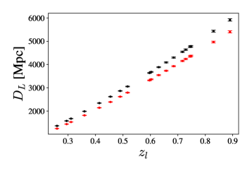
Figure 1: The red points correspond to the $D_{L}$ data obtained by GP considering $M_{b}$ R19, compatible with $H_{0}$ from the Ref. Riess2019 .The black points correspond to the $D_{L}$ data obtained by GP considering $M_{b}$ P18, compatible with $H_{0}$ from the Ref. Planck2019 .

IV.3 Time-Delay

We use a data set of 12 two-image time-delay lensing systems compiled by ibpsc . The use of two-image lensing systems is justified by the consistency with SIS mass profile and its simplicity. However, this selection criterion is necessary but not sufficient to guarantee a SIS mass profile for the lens. Thus, as mentioned in Ref. rana2017 , we include an additional error source denoted by $\zeta$ which takes into consideration possible scatters of individual lenses from a pure SIS mass profile. Moreover, according to Ref. scao2012 $\zeta$ can contribute up to $20\%$ in the $D_{A_{\Delta t}}$ estimation. Adding $\zeta$ quadratically the associated error we obtain

$$\sigma_{D_{A_{\Delta t,0}}}^{2} = D_{A_{\Delta t,0}}^{2}\left\{\Bigg{(}\frac{\sigma_{\Delta t}}{\Delta t}\Bigg{)}^{2}+4\left[\frac{\sigma_{\theta_{A}}\theta_{A}}{(\theta_{B}^{2}-\theta_{A}^{2})}\right]^{2}\right.$$ (20)

$$\left.+4\left[\frac{\sigma_{\theta_{B}}\theta_{B}}{(\theta_{B}^{2}-\theta_{A}^{2})}\right]^{2}+\zeta^{2}\right\},$$

where $\sigma_{\theta_{A}}$ and $\sigma_{\theta_{B}}$ are the errors associated with the source images positions A and B, respectively, and $\sigma_{\Delta t}$ the time-delay error. In addition, we consider seven more time-delay systems obtained by the COSMOGRAIL’s Wellspring (H0LiCOW) collaboration and listed in Table 2 of holicow . Each system were modeled using constraints from high-resolution HST and/or ground-based AO (Adaptive Optics) imaging data (see more details in holicow2 ). Since the data from the Ref. holicow present asymmetric error bars, the data were treated using the method from the Ref. dag (see Fig. 2).

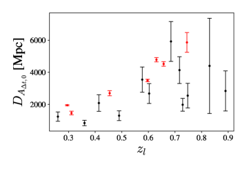
Figure 2: Time-delay angular diameter distance measurements of strong gravitational lensing systems compiled by ibpsc (black points) and holicow (red points).

IV.4 Einstein Radius

We consider a specific catalog containing 158 confirmed sources of strong gravitational lensing presented in Ref. Leaf2018lfu . This compilation includes 118 SGL systems identical to the compilation in Ref. Cao2015 along with 40 new systems recently discovered by SLACS and pre-selected by Shu2017 (see Table I in Ref. Leaf2018lfu ).

However, studies using SGL systems have shown that the pure SIS model may not be an accurate representation of the lens mass distribution when $\sigma_{0}<250$ km/s, for which non-physical values of the quantity $D_{0}$ are usually obtained ($D_{0}>1$). In addition, in Ref. Leaf2018lfu it is mentioned the need for caution when using the SIS model as a reference model, since the impact caused on the density profile can lead to deviations in the observed stellar velocity dispersion ($\sigma_{0}$). It was also observed the need of introducing an additional intrinsic error of approximately $12.22\%$ in order to obtain a better concordance between the data and the $\omega$CDM and $\Lambda$CDM models (see Leaf2018lfu for more details).

Thus, we will consider a general approach to describe the mass distribution of lens-type galaxies, the one in favor of the $\Upsilon$ power-law index model (PLAW), where $\rho\propto r^{-\Upsilon}$. This type of model is important due to several recent studies have shown that the loops of the density profiles of individual galaxies have exhibited a non-negligible spread of the SIS model 1992grlebookS . Thus, the term $D_{0}$ of equation (10) is written by:

$$D_{0}=\frac{e^{4}\theta_{E}}{4\pi\alpha_{0}^{2}\hbar^{2}\sigma_{ap}^{2}}f(\theta_{E},\theta_{ap},\Upsilon),$$ (21)

where $f(\theta_{E},\theta_{ap},\Upsilon)$ is a function which depends on Einstein’s radius ($\theta_{E}$), the angular aperture used by certain gravitational lens Surveys ($\theta_{ap}$), and the power-law index ($\Upsilon$). In the limit $\Upsilon=2$ the SIS model is recovered. Moreover, for a single system we could use the line-of-sight velocity dispersion ($\sigma_{ap}^{2}$), but as we deal with a sample we must transform all the velocity dispersions measured within an aperture into velocity dispersions within circular aperture of radius ($R_{\mathbf{eff}}/2$) following the description 1995MNRAS2761341J : $\sigma_{0}=\sigma_{ap}(\theta_{\mathbf{eff}/(2\theta_{ap})})^{-0.04}$, where $\theta_{\mathbf{eff}}$ is the effective angular radius. In principle, the use of $\sigma_{ap}$ satisfies the model, but the use of $\sigma_{0}$ makes the observable $D_{0}$ more homogeneous for the set of lens located at different redshifts. For that purpose, we just replace $\sigma_{ap}$ for $\sigma_{0}$ in Eq. (21) Cao2015 and, therefore, the corresponding error is given by:

$$\sigma_{D_{0}}^{2} = D_{0}^{2}\left\{4\Bigg{(}\frac{\sigma_{\sigma_{0}}}{\sigma_{0}}\Bigg{)}^{2}+(1-\Upsilon)^{2}\Bigg{(}\frac{\sigma_{\theta_{E}}}{\theta_{E}}\Bigg{)}^{2}+{\zeta^{\prime}}^{2}\right\}.$$ (22)

Here we choose $\Upsilon=2.1$ Ofek:2003sp . Finally, by excluding systems for which the SIS model does not apply and the source J0850-0347 as mentioned in Ref. Leaf2018lfu , the $D_{0}$ final sample is composed by 124 measurements. We apply the GP method to this data set to obtain a reconstructed information of the $D_{0}$ at the same $z$ of time-delay systems. The result of this regression is presented in Fig. 3 (with 1$\sigma$ and 2$\sigma$ intervals).

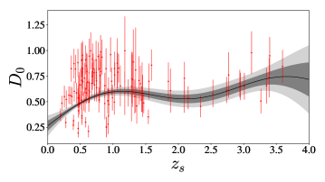
Figure 3: The figure represent an estimate of the ratio $D_{0}$ for PLAW model. The solid black lines represent the central value reconstruction obtained by the Gaussian Process method with the corresponding $1\sigma$ and $2\sigma$ confidence regions.

V Analysis and Discussion

We use Markov Chain Monte Carlo (MCMC) methods to calculate the posterior probability distribution functions (pdf) of the free parameter ($\vec{\Theta}=\gamma$) foreman . Thus, the likelihood distribution function is given by:

$$\mathcal{L}(Data|\vec{\Theta})=\prod\frac{1}{\sqrt{2\pi}\sigma_{\mu}}exp\Bigg{(}-\frac{1}{2}\chi^{2}\Bigg{)},$$ (23)

where

$$\chi^{2}=\sum_{i}\frac{\left[W_{i}-\frac{\phi^{1/2}(z_{l_{i}})}{\phi^{3}(z_{s_{i}})}\right]^{2}}{\sigma_{T_{i}}^{2}},$$ (24)

$$W_{i}\equiv\frac{D_{L_{l_{i}}}}{D_{0,i}D_{A_{\Delta t,0i}}(1+z_{l_{i}})^{2}},$$ (25)

and

$$\sigma_{T_{i}}^{2}=\sigma_{W_{i}}^{2}=\sigma_{D_{0,i}}^{2}+\sigma_{D_{A_{\Delta t,0i}}}^{2}+\sigma_{D_{L_{l_{i}}}}^{2},$$ (26)

the associated total error, $\phi(z_{s})=1-\gamma\ln{(1+z_{s})}$ and $\phi(z_{l})=1-\gamma\ln{(1+z_{l})}$ (where $\gamma$ is the physical parameter of the model). In our analyses, we assume a flat prior as $-1.0\leq\gamma\leq+1.0$.

As one may see in Eq. 25, in order to perform our analyses, it is necessary to obtain the measure of the quantity $D_{0}$ at the redshift of each time-delay system. Then, we use the reconstruction of $D_{0}$ obtained with GP method (see Sec. IV.4). Moreover, in order to obtain a $\chi_{\mathbf{red}}^{2}\approx 1$ (see Eq. 24) in our analyses, it was added an additional intrinsic error ($\sigma_{int}$). We estimate it to be $\approx 33\%$ for ibpsc and $\approx 23\%$ for holicow . For both samples together, $\sigma_{int}$ was estimated to be $\approx 30\%$. The addition of intrinsic error is necessary due to some possible reasons: i) the reported errors are possibly underestimated, and (ii) that there is an additional unrecognized systematic effect that has yet to be included in the analysis as, for instance, possible random deviations from power law model. This kind of approach has been used in previous analyses with SGL systems (see scao2012 ; Leaf2018lfu ).

Our results are as follows (in 1$\sigma$ c.l.):

• By considering $D_{L}$ measurements from the Pantheon compilation with $M_{b}=-19.23\pm 0.04$, we obtain: $\gamma=-0.03_{-0.06}^{+0.05}$ for the 12 time-delay systems ibpsc , and $-0.17_{-0.07}^{+0.06}$ for the 6 time-delay systems holicow . For both samples together: $\gamma=-0.09_{-0.05}^{+0.04}$.

• By considering the $D_{L}$ measurements from Pantheon compilation with $M_{b}=-19.43\pm 0.02$, we obtain: $\gamma=+0.00_{-0.05}^{+0.04}$ for the systems in Ref. ibpsc , and $\gamma=-0.13_{-0.06}^{+0.05}$ considering the systems in Ref. holicow . For both samples together we obtain $\gamma=-0.06_{-0.04}^{+0.04}$ (see Table I).

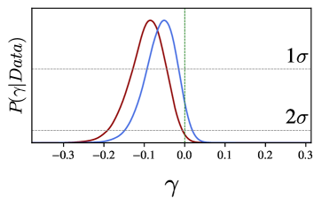
Figure 4: The red and blue contours represent the posterior probability distribution functions for $19$ time-delay Systems from ibpsc ; holicow , but with distinct $D_{L}$ measurements from Pantheon compilation by Riess2019 (red) and Planck2019 (blue). The vertical green dashed line is the limit $\gamma=0$, and the horizontal grey dashed lines represent $1\sigma$ and $2\sigma$ confidence levels.

$D_{L}$ Compilation	time-delay sample	$\gamma(1\sigma)$
Pantheon+R19	ibpsc	$-0.03_{-0.06}^{+0.05}$
Pantheon+P18	ibpsc	$+0.00_{-0.05}^{+0.04}$
Pantheon+R19	holicow	$-0.17_{-0.07}^{+0.06}$
Pantheon+P18	holicow	$-0.13_{-0.06}^{+0.05}$
Pantheon+R19	ibpsc and holicow	$-0.09_{-0.05}^{+0.04}$
Pantheon+P18	ibpsc and holicow	$-0.06_{-0.04}^{+0.04}$

Table 1: Constraints on a possible time variation of the fine-structure constant for the parameter $\gamma$ of the runaway dilaton model in $1\sigma$ of confidence level.

We also performed our analyses with smoothing technique Shafieloo ; Li ; Gonzalez on $D_{0}$ quantity, the results are in full agreement with those by using Gaussian Process.

VI Conclusions

The search for a possible time-space variation of the fundamental constants of nature has raised the interest of many cosmologists due to its possibility of revealing a new underlying physics. In this context, we provided a new method capable of probing a possible temporal evolution of the fine-structure constant by considering time-delay of Strong Gravitational Lensing Systems. A possible temporal variation of $\alpha$ ($\alpha=\alpha_{0}\phi(z)$) was investigated in a class of runaway dilaton models, where $\phi(z)=1-\gamma\ln(1+z)$, where $\gamma$ is a free parameter.

The most restrictive bounds come from the joint analysis using the two samples of time-delay systems together from the Refs. ibpsc and holicow . We obtained $\gamma=-0.09_{-0.05}^{+0.04}$ and $\gamma=-0.06_{-0.04}^{+0.04}$ for $D_{L}$ measurements from Pantheon+R19 and Pantheon+P18, respectively (see Fig. 4 and Table I).

Finally, it is important to stress that recently the authors in the Ref. Lee:2021kjr showed that fitting turbulent models in quasars necessarily generates or enhances model non-uniqueness, adding a substantial additional random uncertainty to $\Delta\alpha/\alpha$ obtained from quasar absorption systems. Basically, any given absorption system can be fitted equally well by many slightly different models, each furnishing a different value to $\frac{\Delta\alpha}{\alpha}$. Therefore, although SGL plus time-delay systems are not as much competitive as the limits imposed by quasar absorption systems, the constraints imposed in this paper provide new and independent limits on a possible temporal variation of the fine-structure constant.

VII Acknowledgments

The authors thank to Brazilian scientific and financial support federal agencies, CAPES, and CNPq. RFLH thanks to CNPq No.428755/2018-6 and 305930/2017-6.

References

- (1) P. A. M. Dirac, “The cosmological constants”, Nature 139, 323 (1937).
- (2) J. P. Uzan, “Varying Constants, Gravitation and Cosmology”, Living Rev. Rel. 14, 2 (2011) [arXiv:1009.5514].
- (3) C. J. A. P. Martins, “The status of varying constants: a review of the physics, searches and implications”, [arXiv:1709.02923].
- (4) S. Ray, U. Mukhopadhyay, S. Ray, & A. Bhattacharjee, “Dirac’s large number hypothesis: A journey from concept to implication”, Int. J. Mod. Phys. D 28, 08 (2019).
- (5) J. D. Bekenstein, “Fine-structure constant: Is it really a constant?”, PRD 25, 6 (1982).
- (6) H. B. Sandvik, J. D. Barrow, & J. Magueijo, “A simple cosmology with a varying fine-structure constant”, PRL 88, 3 (2002) [astro-ph/0107512].
- (7) J. D. Barrow, & S.Z.W. Lip, “A Generalized Theory of Varying Alpha”, PRD 85, 023514 (2012) [arXiv:1110.3120].
- (8) J. D. Barrow, & A. A. H. Graham, “General Dynamics of Varying-Alpha Universes”, PRD 88, 10 (2013) [arXiv:1307.6816].
- (9) M. Dine, W. Fischler, & M. Srednicki, “A simple solution to the strong CP problem with a harmless axion”, PLB 104, 3 (1981); D. B. Kaplan, “Opening the axion window”, NPB 260, 1 (1985).
- (10) P. Brax, et al., “Detecting dark energy in orbit: The cosmological chameleon”, PRF 70, (2004) [arXiv:astro-ph/0408415v2]; P. Brax, C. Van de Bruck, & A. C. Davies, “Compatibility of the ChameleonField Model with Fifth-Force Experiments, Cosmology, and PVLAS and CAST Results”, PRL 99, 12 (2007) [arXiv:hep-ph/0703243v2]; M. Ahlers, A. Lindner, A. Ringwald, L. Schrempp, & C. Weniger, “Alpenglow: A signature for chameleons in axionlike particle search experiments”, PRD 77, 1 (2008) [arXiv:0710.1555v1]; J. Khoury, & A. Weltman, “Chameleon Cosmology”, PRD 69, 4 (2004) [arXiv:astro-ph/0309411v2].
- (11) A. Chodos, & S.L. Detweiler, “Where has the fifth dimension gone?”, PRD 21, 8 (1980).
- (12) Y.S. Wu, & Z. Wang, “Essay on gravitation: Present-time variation of Newton’s gravitational constant in superstring theories”, PRL20, 1 (1988).
- (13) E. Kiritsis, “Supergravity, D-brane probes and thermal superYang-Mills: A Comparison”, JHEP 10, 010 (1999) [arXiv:hep-th/9906206].
- (14) S. J. Landau, “Variation of fundamental constants and white dwarfs”, (2020) [arXiv:2002.00095].
- (15) M. B Bainbridge, and others, “Probing the Gravitational Dependence of the Fine-Structure Constant from Observations of White Dwarf Stars”, Universe 3, 2 (2017) [arXiv:1702.01757].
- (16) M. R. Wilczynska, and others, “Four direct measurements of the fine-structure constant 13 billion years ago”, (2020) [arXiv:2003.07627].
- (17) J. K. Webb, and others, “Search for Time Variation of the Fine-Structure Constant”, PRL 82, 5 [astro-ph/9803165].
- (18) W. Ubachs, “Search for varying constants of nature from astronomical observation of molecules”, Space Sce. Rev. 214, 1 (2018) [arXiv:1709.07704].
- (19) C.-C. Lee, J. K. Webb, D. Milaković, R. F. Carswell, “Non-uniqueness in quasar absorption models and implications for measurements of the fine-structure constant”, (2021) [arXiv:2102.11648].
- (20) L. Hart, & J. Chluba, “Updated fundamental constant constraints from Planck 2018 data and possible relations to the Hubble tension”, MNRAS 493, 3 (2020) [arXiv:1912.03986].
- (21) Aghanim, N. and others, “Planck 2018 results. V. CMB power spectra and likelihoods”, A&A 641, A5 (2020) [arXiv:1907.12875].
- (22) Aghanim, N. and others, “Planck 2018 results. VIII. Gravitational lensing”, A&A 641, A8 (2020) [arXiv:1807.06210].
- (23) Ade, P.A.R. and others, “Planck intermediate results - XXIV. Constraints on variations in fundamental constants”, A&A 580, A22 (2015) [arXiv:1406.7482].
- (24) T. L. Smith, D. Grin, D. Robinson, & D. Qi, “Probing spatial variation of the fine-structure constant using the CMB”, PRD 99, 4 (2018) [arXiv:1808.07486].
- (25) A. Hess, and others, “Search for a Variation of the Fine-Structure Constant around the Supermassive Black Hole in Our Galactic Center”, PRL 124, 8 (2020) [arXiv:2002.11567].
- (26) S. Galli, “Clusters of galaxues and variation of the fine-structure constant”, PRD 87, 12 (2013) [arXiv:1212.1075v1].
- (27) M. T. Clara, & C. J. A. P. Martins, “Primordial nucleosynthesis with varying fundamental constants: Improved constraints and a possible solution to the Lithium problem”, A&A 633, L11 (2020), [arXiv:2001.01787].
- (28) D. Milaković, C.-C. Lee, R. F. Carswell, J. K. Webb, P. Molaro, & L. Pasquini, “A new era of fine-structure constant measurements at high redshift”, (2020) [arXiv:2008.10619].
- (29) L. Kraiselburd, F. L. Castillo, M. E. Mosquera, & H. Vucetich, “Magnetic contributions in Bekenstein type models”, PRD 97, 4 (2018) [arXiv:1801.08594].
- (30) J.-J. Zhang, L. Yin, & C.-Q. Geng, “Cosmological constraints on CDM models with time-varying fine-structure constant”, Annals Phys. 397, 400–409 (2018) [arXiv:1809.04218].
- (31) H. Wein, X.-B. Zou, H.Y. Li, & D.Z. Xue, “Cosmological constant, fine-structure constant and beyond”, Eur. Phys. J. C 77, 1 (2017) [arXiv:1605.04571].
- (32) N. Hinkley, J. A. Sherman, N. B. Phillips, M. Schioppo, N. D. Lemke, K. Beloy, M. Pizzocaro, C. W. Oates, & A. D. Ludlow, “An Atomic Clock with Instability”, Science 341, 6151 (2013) [arXiv:1305.5869].
- (33) E. A. Dijck, “Spectroscopy of Trapped 138Ba+ Ions for Atomic Parity Violation and Optical Clocks”, (2020).
- (34) T. Damour, F. Piazza, & G. Veneziano, “Violations of the equivalence principle in a dilaton-runaway scenario”, PRD 66, 4 (2002) [arXiv:hep-th/0205111v2].
- (35) T. Damour, F. Piazza, & G. Veneziano, “Runaway Dilaton and Equivalence Principle Violations”, PRL 89, 8 (2002) [arXiv:gr-qc/0204094v2].
- (36) R. F. L. Holanda, L. R. Colaço, R. S. Gonalves, & J. S. Alcaniz, “Limits on evolution of the fine-structure constant in runaway dilaton models from Sunyaev-Zeldovich Observation”, PLB 767, 188-192 (2017) [arXiv:1701.07250].
- (37) L. R. Colaço, R. F. L. Holanda, R. Silva, & J. S. Alcaniz, “Galaxy clusters and a possible variation of the fine-structure constant”, JCAP 03, 014 (2019) [arXiv:1901.10947].
- (38) K. Bora, & S. Desai, “Constraints on variation of the fine-structure constant from joint SPT-SZ and XMM-Newton observations”, (2020) [arXiv:2008.10541].
- (39) L. R. Colaço, R. F. L. Holanda, & R. Silva, “Probing variation of the fine-structure constant using the strong gravitational lensing”, (2020) [arXiv:2004.08484].
- (40) R. F. L. Holanda, S. J. Landau, J. S. Alcaniz, I. E. Sanchez, & V. C. Busti, “Constraints on a possible variation of the fine-structure constant from galaxy cluster data”, JCAP 1605, 047 (2016) [arXiv:1510.07240].
- (41) R. F. L. Holanda, V. C. Busti, L. R. Colaço, J. S. Alcaniz, & S. J. Landau, “Galaxy clusters, type Ia supernovae and the fine-structure constant”, JCAP 1608, 055 (2016) [arXiv:1605.02578].
- (42) I. Balmès, & P. S. Corasaniti, “Bayesian approach to gravitational lens model selection: constraining H0 with a selected sample of strong lenses”, MNRAS 431, 2 (2013) [arXiv:1206.5801].
- (43) S. Birrer, et al., “TDCOSMO - IV. Hierarchical time-delay cosmography – joint inference of the Hubble constant and galaxy density profiles”, Astron. Astrophys. 643, A165 (2020) [arXiv:2007.02941].
- (44) D. M. Scolnic, et al., “The complete Ligh-curve Sample of Spectroscopically Confirmed SNe Ia from Pan-STARRS1 and Cosmological Constraints from the Combined Pantheon Sample”, ApJ 859, 101 (2018) [arXiv:1710.00845].
- (45) K. Leaf, & F. Melia, “Model selection with strong-lensing systems”, MNRAS 478, 4 (2018) [arXiv:1805.08640].
- (46) A. Hess, O. Minazzoli, & J. Larena, “Observables in theories with a varying fine-structure constant”, Gen. Rel. Grav. 47, 2 (2015) [arXiv:1409.7273].
- (47) O. Hees, A. Minazzoli, & J. Larena, “Breaking of the equivalence principle in the electromagnetic sector and its cosmological signatures”, PRD 90, 12 (2014) [arXiv:1406.6187v4].
- (48) S. Cao, M. Biesiada, & R. Gavazzi, “Cosmology with Strong-Lensing Systems”, ApJ 806, 2 (2015) [arXiv:1509.07649].
- (49) P. Schneiner, J. Ehlers, & E. E. Falco, “Gravitational Lenses”, Springer-Verlag Berlin Heidelberg New York. Also Astronomy and Astrophysics Library 2019.
- (50) S. Refsdal, “On the possibility of determining Hubble’s parameter and the masses of galaxies from the gravitational lens effect”, MNRAS 128, 307 (1964).
- (51) S.H. Suyu, et al., “Dissecting the Gravitational lens B1608+656. II. Precision Measurements of the Hubble Constant, Spatial Curvature, and the Dark Energy Equation of State”, ApJ 711, 1 (2009) [arXiv:0910.2773].
- (52) T. Treu, “Strong Lensing by Galaxies”, ARAA 48, 87-125 (2010) [arXiv:1003.5567].
- (53) S. H. Suyu et al., “Dissecting the Gravitational lens B1608+656. II. Precision Measurements of the Hubble Constant, Spatial Curvature, and the Dark Energy Equation of State”, ApJ 711, 201-125 (2010).
- (54) J.-L. Wei, X.-F. Wu, & F. Melia, “A Comparison of Cosmological Models Using Time Delay Lenses”, ApJ 788, 190 (2014) [arXiv:1405.2388].
- (55) O. Minazzoli, & A. Hees, “Late-time cosmology of a scalar-tensor theory with a universal multiplicative coupling between the scalar field and the matter Lagrangian”, PRD 90, 2 (2014) [arXiv:1404.4266v2].
- (56) B. Xu, and Q. Huang, “New tests of the cosmic distance duality relation with the baryon acoustic osculattion and type Ia supernovae”, The Eur. Phys. J. P. 135, 06 (2020).
- (57) C. Ma, & P.-S. Corasaniti, “Statistical Test of Distance-Duality Relation with Type Ia Supernovae and Baryon Acoustic Oscillatuion”, ApJ 861, 2 (2018) [arXiv:1604.04631].
- (58) M. Seikel, C. Clarkson, “Optimising Gaussian processes for reconstructing dark energy dynamics from supernovae”, (2013) [arXiv:1311.6678].
- (59) A. G. Riess, S. Casertano, W. Yuan, L. M. Macri, D. Scolnic, “Large Magellanic Cloud Cepheid Standards Provide a 1% Foundation for the Determination of the Hubble Constant and Stronger Evidence for Physics beyond CDM”, Astrophys. J. 876, 1 (2019) [arXiv:1903.07603].
- (60) N. Aghanim, and others, “Planck 2018 results. VI. Cosmological parameters”, Astron. Astrophys. 641, A6 (2020) [arXiv:1807.06209].
- (61) A. Rana, D. Jain, S. Mahajan, A. Mukherjee, & R. F. L. Holanda, “Probing the cosmic distance duality relation using time delay lenses”, JCAP 07, 010 (2017) [arXiv:1705.04549].
- (62) S. Cao, Y. Pan, M. Biesiada, W. Godlowski, & Z.-H. Zhu, “Constraints on cosmological models from strong gravitational lensing systems”, JCAP 2012, 3 (2012) [arXiv:1105.6226].
- (63) S. Birrer, and others, “TDCOSMO - IV. Hierarchical time-delay cosmography – joint inference of the Hubble constant and galaxy density profiles”, Astron. Astrophys. 643, A165 (2020) [arXiv:2007.02941]; K. C. Wong, and others, “H0LiCOW – XIII. A 2.4 per cent measurement of H0 from lensed quasars: 5.3 tension between early- and late-Universe probes”, Mon. Not. Roy. Astron. Soc. 498, 1 (2020) [1907.04869].
- (64) D’Agostini, G., “Asymetric uncertainties: Sources, treatment and potential dangers”, (2004) [physics/0403086].
- (65) Y. Shu, et al., “The Sloan Lens ACS Survey. XIII. Discovery of 40 New Galaxy-scale Strong Lenses”, ApJ 851, 1 (2017) [arXiv:1711.00072].
- (66) P. Schneider, J. Ehlers, & E. E. Falco, “Gravitational Lenses”, Springer Science & Business Media (1999).
- (67) I. Jorgensen, M. Franx, & P. Kjaergaard, “Spectroscopy for E and S0 galaxies in nine clusters”, MNRAS 276, 4 (1995).
- (68) E. O. Ofek, H.-W. Rix, & D. Maoz, “The redshift distribution of gravitational lenses revisited: Constraints on galaxy mass evolution”, MNRAS 343, 639 (2003) [astro-ph/0305201].
- (69) D. Foreman-Mackey, D. W. Hogg, D. Lang, & J. Goodman, “emcee: The MCMC Hammer”, Publ. Astron. Soc. Pac. 125, 925 (2013) [arXiv:1202.3665].
- (70) A. Shafieloo, U. Alam, V. Sahni, & A. Starobinsky, “Smoothing Supernova Data to Reconstruct the Expansion History of the Universe and its Age”, MNRAS 366, 1081 (2006)[arXiv:0505329].
- (71) Li, Zhengxiang and Gonzalez, J. E. and Yu, Hongwei and Zhu, Zong-Hong and Alcaniz, J. S.”, “Constructing a cosmological model-independent Hubble diagram of type Ia supernovae with cosmic chronometers”, Phys. Rev. D 93, 4 (2016) [arXiv:1504.03269].
- (72) Gonzalez, J. E. and Alcaniz, J. S. and Carvalho, J. C.,” Smoothing expansion rate data to reconstruct cosmological matter perturbations”, JCAP 08, 008 (2017) [arXiv:1702.02923].