DiffTune: Optimizing CPU Simulator Parameters with Learned Differentiable Surrogates

Abstract

CPU simulators are useful tools for modeling CPU execution behavior. However, they suffer from inaccuracies due to the cost and complexity of setting their fine-grained parameters, such as the latencies of individual instructions. This complexity arises from the expertise required to design benchmarks and measurement frameworks that can precisely measure the values of parameters at such fine granularity. In some cases, these parameters do not necessarily have a physical realization and are therefore fundamentally approximate, or even unmeasurable.

In this paper we present DiffTune, a system for learning the parameters of x86 basic block CPU simulators from coarse-grained end-to-end measurements. Given a simulator, DiffTune learns its parameters by first replacing the original simulator with a differentiable surrogate, another function that approximates the original function; by making the surrogate differentiable, DiffTune is then able to apply gradient-based optimization techniques even when the original function is non-differentiable, such as is the case with CPU simulators. With this differentiable surrogate, DiffTune then applies gradient-based optimization to produce values of the simulator’s parameters that minimize the simulator’s error on a dataset of ground truth end-to-end performance measurements. Finally, the learned parameters are plugged back into the original simulator.

DiffTune is able to automatically learn the entire set of microarchitecture-specific parameters within the Intel x86 simulation model of llvm-mca, a basic block CPU simulator based on LLVM’s instruction scheduling model. DiffTune’s learned parameters lead llvm-mca to an average error that not only matches but lowers that of its original, expert-provided parameter values.

I Introduction

Simulators are widely used for architecture research to model the interactions of architectural components of a system [1, 2, 3, 4, 5, 6]. For example, CPU simulators, such as llvm-mca [2], and llvm_sim [7], model the execution of a processor at various levels of detail, potentially including abstract models of common processor design concepts such as dispatch, execute, and retire stages [8]. CPU simulators can operate at different granularities, from analyzing just basic blocks, straight-line sequences of assembly code instructions, to analyzing whole programs. Such simulators allow performance engineers to reason about the execution behavior and bottlenecks of programs run on a given processor.

However, precisely simulating a modern CPU is challenging: not only are modern processors large and complex, but many of their implementation details are proprietary, undocumented, or only loosely specified even given the thousands of pages of vendor-provided documentation that describe any given processor. As a result, CPU simulators are often composed of coarse abstract models of a subset of processor design concepts. Moreover, each constituent model typically relies on a number of approximate design parameters, such as the number of cycles it takes for an instruction to pass through the processor’s execute stage. Choosing an appropriate level of model detail for simulation, as well as setting simulation parameters, requires significant expertise. In this paper, we consider the challenge of setting the parameters of a CPU simulator given a fixed level of model detail.

Measurement

One methodology for setting the parameters of such a CPU simulator is to gather fine-grained measurements of each individual parameter’s realization in the physical machine [9, 10] and then set the parameters to their measured values [11, 12]. When the semantics of the simulator and the semantics of the measurement methodology coincide, then these measurements can serve as effective parameter values. However, if there is a mismatch between the simulator and the measurement methodology, then measurements may not provide effective parameter settings [13, Section 5.2]. Moreover, some parameters may not correspond to measurable values.

Optimizing simulator parameters

An alternative to developing detailed measurement methodologies for individual parameters is to infer the parameters from coarse-grained end-to-end measurements of the performance of the physical machine [13]. Specifically, given a dataset of benchmarks, each labeled with their true behavior on a given CPU (e.g., with their execution time or with microarchitectural events, such as cache misses), identify a set of parameters that minimize the error between the simulator’s predictions and the machine’s true behavior. This is generally a discrete, non-convex optimization problem for which classic strategies, such as random search [14], are intractable because of the size of the parameter space (approximately $10^{19336}$ possible parameter settings in one simulator, llvm-mca).

Our approach: DiffTune

In this paper, we present DiffTune, an optimization algorithm and implementation for learning the parameters of programs. We use DiffTune to learn the parameters of x86 basic block CPU simulators.

DiffTune’s algorithm takes as input a program, a description of the program’s parameters, and a dataset of input-output examples describing the program’s desired output, then produces a setting of the program’s parameters that minimizes the discrepancy between the program’s actual and desired output. The learned parameters are then plugged back into the original program.

The algorithm solves this optimization problem via a differentiable surrogate for the program [15, 16, 17, 18, 19]. A surrogate is an approximation of the function from the program’s parameters to the program’s output. By requiring the surrogate to be differentiable, it is then possible to compute the surrogate’s gradient and apply gradient-based optimization [20, 21] to identify a setting of the program’s parameters that minimize the error between the program’s output (as predicted by the surrogate) and the desired output.

To apply this to basic block CPU simulators, we instantiate DiffTune’s surrogate with a neural network that can mimic the behavior of a simulator. This neural network takes the original simulator input (e.g., a sequence of assembly instructions) and a set of proposed simulator parameters (e.g., dispatch width or instruction latency) as input, and produces the output that the simulator would produce if it were instantiated with the given simulator’s parameters. We derive the neural network architecture of our surrogate from that of Ithemal [22], a basic block throughput estimation neural network.

Results

Using DiffTune, we are able to learn the entire set of 11265 microarchitecture-specific parameters in the Intel x86 simulation model of llvm-mca [2]. llvm-mca is a CPU simulator that predicts the execution time of basic blocks. llvm-mca models instruction dispatch, register renaming, out-of-order execution with a reorder buffer, instruction scheduling based on use-def latencies, execution by dispatching to ports, a load/store unit ensuring memory consistency, and a retire control unit.

We evaluate DiffTune on four different x86 microarchitectures, including both Intel and AMD chips. Using only end-to-end supervision of the execution time measured per-microarchitecture of a large dataset of basic blocks from Chen et al. [23], we are able to learn parameters from scratch that lead llvm-mca to have an average error of $24.6\%$, down from an average error of $30.0\%$ with llvm-mca’s expert-provided parameters. In contrast, black-box global optimization with OpenTuner [14] is unable to identify parameters with less than $100\%$ error.

Contributions

We present the following contributions:

• We present DiffTune, an algorithm for learning ordinal parameters of programs from input-output examples.

• We present an implementation of DiffTune for x86 basic block CPU simulators that uses a variant of the Ithemal model as a differentiable surrogate.

• We evaluate DiffTune on llvm-mca and demonstrate that DiffTune can learn the entire set of microarchitectual parameters in llvm-mca’s Intel x86 simulation model.

• We present case studies of specific parameters learned by DiffTune. Our analysis demonstrates cases in which DiffTune learns semantically correct parameters that enable llvm-mca to make more accurate predictions. Our analysis also demonstrates cases in which DiffTune learns parameters that lead to higher accuracy but do not correspond to reasonable physical values on the CPU.

Our results show that DiffTune offers the promise of a generic, scalable methodology to learn detailed performance models with only end-to-end measurements, reducing performance optimization tasks to simply that of gathering data.

II Background: Simulators

Simulators comprise a large set of tools for modeling the execution behavior of computing systems, at all different levels of abstraction: from cycle-accurate simulators to high-level cost models. These simulators are used for a variety of applications:

• gem5 [1] is a detailed, extensible full system simulator that is frequently used for computer architecture research, to model the interaction of new or modified components with the rest of a CPU and memory system.

• IACA [3] is a static analysis tool released by Intel that models the behavior of modern Intel processors, including undocumented Intel CPU features, predicting code performance. IACA is used by performance engineers to diagnose and fix bottlenecks in hand-engineered code snippets [24].

• LLVM [25] includes internal CPU simulators to predict the performance of generated code [26, 27]. LLVM uses these CPU simulators to search through the code optimization space, to generate more optimal code.

Though these simulators are all simplifications of the true execution behavior of physical systems, they are still highly complex pieces of software.

II-A llvm-mca

For example, consider llvm-mca [2], an out-of-order superscalar CPU simulator included in the LLVM [25] compiler infrastructure. The main design goal of llvm-mca is to expose LLVM’s instruction scheduling model for testing. llvm-mca takes basic blocks as input, sequences of straight-line assembly instructions with no branches, jumps, or loops. For a given input basic block, llvm-mca predicts the timing of 100 repetitions of that block, measured in cycles.

Design

llvm-mca is structured as a generic, target-independent simulator parameterized on LLVM’s internal model of the target hardware. llvm-mca makes two core modeling assumptions. First, it assumes that the simulated program is not bottlenecked by the processor frontend; in fact, llvm-mca ignores instruction decoding entirely. Second, llvm-mca assumes that memory data is always in the L1 cache, and ignores the memory hierarchy.

llvm-mca simulates a processor in four main stages: dispatch, issue, execute, and retire. The dispatch stage reserves physical resources (e.g., slots in the reorder buffer) for each instruction, based on the number of micro-ops the instruction is composed of. Once dispatched, instructions wait in the issue stage until they are ready to be executed. The issue stage blocks an instruction until its input operands are ready and until all of its required execution ports are available. Once the instruction’s operands and ports are available, the instruction enters the execute stage. The execute stage reserves the instruction’s execution ports and holds them for the durations specified by the instruction’s port map assignment specification. Finally, once an instruction has executed for its duration, it enters the retire stage. In program order, the retire stage frees the physical resources that were acquired for each instruction.

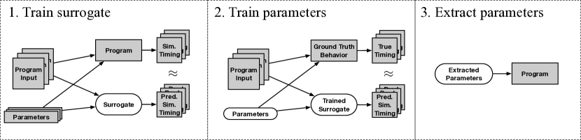
Figure 1: DiffTune block diagram.

TABLE I: Terms used in formalism in Section III.

Notation	Definition
$f$	Program that we are trying to optimize.
$\theta$	Parameters of the program that we are trying to optimize.
$x$	Input to the program.
$y$	Output of the program on an input $x$.
$\mathcal{I}$	Dataset of program inputs to optimize against.
$f^{*}$	Ground truth behavior that we are trying to model with $f$.
$\mathcal{L}$	Loss function describing the error of a proposed solution.
$\hat{f}$	The surrogate, which is trained to model the original program: $\hat{f}\approx f$.
$D$	Distribution that parameters $\theta$ are sampled from for training the surrogate.

Parameters

Each stage in llvm-mca’s model requires parameters. The NumMicroOps parameter for each instruction specifies how many micro-ops the instruction is composed of. The DispatchWidth parameter specifies how many micro-ops can enter and exit the dispatch stage in each cycle. The ReorderBufferSize parameter specifies how many micro-ops can reside in the issue and execute stages at the same time. The PortMap parameters for each instruction specify the number of cycles for which the instruction occupies each execution port. An additional WriteLatency parameter for each instruction specifies the number of cycles before destination operands of that instruction can be read from, while ReadAdvanceCycles parameters for each instruction specify the number of cycles by which to accelerate the WriteLatency of source operands (representing forwarding paths).

In sum, the $837$ instructions in our dataset (Section V-A) lead to $11265$ total parameters with $10^{19336}$ possible configurations in llvm-mca’s Haswell microarchitecture simulation.

II-B Challenges

These parameter tables are currently manually written for each microarchitecture, based on processor vendor documentation and manual timing of instructions. Specifically, many of LLVM’s WriteLatency and PortMap parameters are drawn from the Intel optimization manual [28, 29], Agner Fog’s instruction tables [9, 11], and uops.info [10, 12], all of which contain latencies and port mappings for assembly instructions across different architectures and microarchitectures.

Measurability

However, these documented and measured values do not directly correspond to parameters in llvm-mca, because llvm-mca’s parameters, and abstract simulator parameters more broadly, are not defined such that they have a single measurable value. For instance, llvm-mca defines exactly one WriteLatency parameter per instruction. However, Fog [9] and Abel and Reineke [10] find that for instructions that produce multiple results in different destinations, the results might be available at different cycles. Further, the latency for results to be available can depend on the actual value of the input operands. Thus, there is no single measurable value that corresponds to llvm-mca’s definition of WriteLatency.

Different choices for how to map from measured latencies to WriteLatency values result in different overall errors (as defined in Section V-A). For instance, when llvm-mca is instantiated with Abel and Reineke [10]’s maximum observed latency for each instruction, llvm-mca gets an error of $218\%$ when generating predictions for the Haswell microarchitecture; the median observed latency results in an error of $150\%$; and the minimum observed latency results in an error of $103\%$.

III Approach

Tuning llvm-mca’s $11265$ parameters among $10^{19336}$ valid configurations2 by exhaustive search is impractical. Instead, we present DiffTune, an algorithm for learning ordinal parameters of arbitrary programs from labeled input and output examples. DiffTune leverages learned differentiable surrogates to make the optimization process more tractable.

Formal problem statement

Given a program $f:\Theta\to\mathcal{X}\to\mathcal{Y}$ parameterized on parameters $\theta:\Theta$, that takes inputs $x:\mathcal{X}$ to outputs $y:\mathcal{Y}$, and given a function $f^{*}:\mathcal{X}\to\mathcal{Y}$ that represents ground-truth behavior, find parameters $\theta\in\Theta$ to minimize the expected value of a cost function (called the loss function, representing error) $\mathcal{L}:\mathopen{}\mathclose{{}\left(\mathcal{Y}\times\mathcal{Y}}\right)\to\mathbb{R}_{\geq 0}$ of the discrepancy between the behavior of the program $f$ and the ground-truth behavior $f^{*}$ on a dataset of program inputs $\mathcal{I}\subseteq\mathcal{X}$:

$$\operatorname*{arg\,min}_{\theta}\mathbb{E}_{x\sim\mathcal{I}}\mathopen{}\mathclose{{}\left[\mathcal{L}\mathopen{}\mathclose{{}\left(f\mathopen{}\mathclose{{}\left(\theta,x}\right),f^{*}\mathopen{}\mathclose{{}\left(x}\right)}\right)}\right]$$ (1)

Algorithm

Figure 1 presents a diagram of our approach. We first optimize the surrogate $\hat{f}:\Theta\to\mathcal{X}\to\mathcal{Y}$ to mimic the original program, i.e., $\forall\theta,x.\hat{f}(\theta,x)\approx f(\theta,x)$. Specifically, we optimize the surrogate to minimize the expectation of the loss $\mathcal{L}$ over program inputs from $\mathcal{I}$ and samples of $\theta$ from a pre-defined parameter sampling distribution $D$:

$$\operatorname*{arg\,min}_{\hat{f}}\mathbb{E}_{x\sim\mathcal{I},\theta\sim D}\mathopen{}\mathclose{{}\left[\mathcal{L}\mathopen{}\mathclose{{}\left(f\mathopen{}\mathclose{{}\left(\theta,x}\right),\hat{f}\mathopen{}\mathclose{{}\left(\theta,x}\right)}\right)}\right]$$ (2)

We then optimize the parameters $\theta$ to minimize the discrepancy between predictions of the surrogate $\hat{f}$ and the ground-truth behavior $f^{*}$. Specifically, we find:

$$\operatorname*{arg\,min}_{\theta}\mathbb{E}_{x\sim\mathcal{I}}\mathopen{}\mathclose{{}\left[\mathcal{L}\mathopen{}\mathclose{{}\left(\hat{f}\mathopen{}\mathclose{{}\left(\theta,x}\right),f^{*}\mathopen{}\mathclose{{}\left(x}\right)}\right)}\right]$$ (3)

Finally, we extract the learned parameters $\theta$ from the optimization problem and plug them into the original program $f$, applying any constraints (e.g., that the parameters must be integers) that were not enforced when optimizing against the surrogate.

Discussion

Note the similarity between Equation 1 and Equation 3: the two equations only differ by the use of $f$ and $\hat{f}$, respectively. The close correspondence between forms makes clear that $\hat{f}$ stands in as a surrogate for the original program, $f$. This is a general algorithmic approach [15] that is desirable when it is possible to choose $\hat{f}$ such that it is easier or more efficient to optimize $\theta$ using $\hat{f}$ than $f$.

Optimization

In our approach, we choose $\hat{f}$ to be a neural network. Neural networks are typically built as compositions of differentiable architectural components, such as embedding lookup tables, which map discrete input elements to real-valued vectors; LSTMs [30], which map input sequences of vectors to a single output vector; and fully connected layers, which are linear transformations on input vectors. By being composed of differentiable components, neural networks are end-to-end differentiable, so that they are able to be trained using gradient-based optimization. Specifically, neural networks are typically optimized with stochastic first-order optimizations like stochastic gradient descent (SGD) [20], which repeatedly calculates the network’s error on a small sample of the training dataset and then updates the network’s parameters in the opposite of the direction of the gradient to minimize the error.

By selecting a neural network as $\hat{f}$’s representation, we are able to leverage $\hat{f}$’s differentiable nature not only to train $\hat{f}$ (solving the optimization problem posed in Equation 2) but also to solve the optimization problem posed in Equation 3 with gradient-based optimization. This stands in contrast to $f$ which is, generally, non-differentiable and therefore does not permit the computation of its gradients.

Surrogate example

A visual example of this is presented in Figure 2, which shows an example of the timing predicted by llvm-mca (blue) and a trained surrogate of llvm-mca (orange). The x-axis of Figure 2 is the value of the DispatchWidth parameter, and the y-axis is the predicted timing of llvm-mca with that DispatchWidth for the basic block consisting of the single instruction shrq $5, 16(%rsp). The blue points represent the prediction of llvm-mca when instantiated with different values for DispatchWidth. The naïve approach of optimizing llvm-mca would be combinatorial search, since without a continuous and smooth surface to optimize, it is impossible to use standard first-order techniques. DiffTune instead first learns a surrogate of llvm-mca, represented by the orange line in Figure 2. This surrogate, though not exactly the same as llvm-mca, is smooth and differentiable. Importantly, the surrogate interpolates llvm-mca’s predictions even in places where llvm-mca does not have a defined output, such as between the integer-valued parameter settings. Together, these properties mean that it is possible to optimize parameters against the surrogate with first-order techniques like gradient descent.

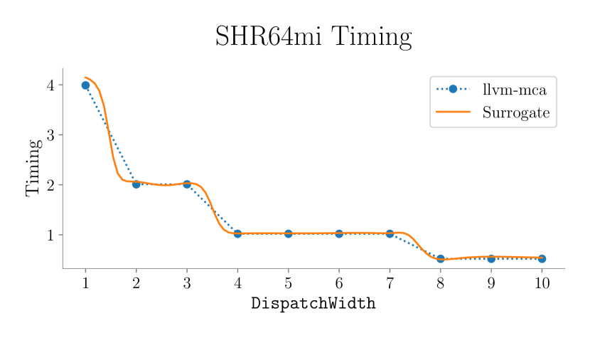
Figure 2: Example of timing predicted by llvm-mca (blue) and a surrogate (orange), while varying DispatchWidth. By learning the surrogate, we are able to optimize the parameter value with gradient descent, rather than requiring combinatorial search.

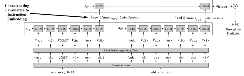
Figure 3: Design of the surrogate, from Mendis et al. [22] with added parameter inputs. We use $\parallel$ to denote concatenation of parameters to the instruction embedding.

IV Implementation

This section discusses our implementation of DiffTune, available online at https://github.com/ithemal/DiffTune.

Parameters

We consider two types of parameters that we optimize with DiffTune: per-instruction parameters, which are a uniform length vector of parameters associated with each individual instruction opcode (e.g. for llvm-mca, a vector containing WriteLatency, NumMicroOps, etc.); and global parameters, which are a vector of parameters that are associated with the overall simulator behavior (e.g. for llvm-mca, a vector containing the DispatchWidth and ReorderBufferSize). We further support two types of constraints in our implementation: lower-bounded, specifying that parameter values cannot be below a certain value (often $0$ or $1$), and integer-valued, specifying that parameter values must be integers. During optimization, all parameters are represented as floating-point.

Surrogate design

Figure 3 presents our surrogate design, which is capable of learning parameters for x86 basic block performance models such as llvm-mca.

We use a modified version of Ithemal [22], a learned basic block performance model, as the surrogate. In the standard implementation of Ithemal (without our modifications), Ithemal first uses an embedding lookup table to map the opcode and operands of each instruction into vectors. Next, Ithemal processes the opcode and operand embeddings for each instruction with an LSTM, producing a vector representing each instruction. Then, Ithemal processes the sequence of instruction vectors with another LSTM, producing a vector representing the basic block. Finally, Ithemal uses a fully connected layer to turn the basic block vector into a single number representing Ithemal’s prediction for the timing of that basic block.

We modify Ithemal in two ways to act as the surrogate. First, we replace each individual LSTM with a set of 4 stacked LSTMs, a common technique to increase representative capacity [31], to give Ithemal the capacity to represent the dependency of the prediction on the input parameters as well as on the input basic block. Second, to provide the parameters as input we concatenate the per-instruction parameters and the global parameters to each instruction vector before processing the instruction vectors with the instruction-level LSTM.

Solving the optimization problems

Training the surrogate requires first defining sampling distributions for each parameter (e.g., a bounded uniform distribution on integers). We then generate a large simulated dataset by repeatedly sampling a basic block from the ground-truth dataset, sampling a parameter table from the defined sampling distributions, instantiating the simulator with the parameter table, and generating a prediction for the basic block. We train the surrogate using SGD against this simulated dataset. During surrogate training, for parameters constrained to be lower-bounded we subtract the lower bound before passing them as input to the surrogate.

To train the parameter table, we first initialize it to a random sample from the parameter sampling distribution. We generate predictions using the parameter table plugged into the trained surrogate, and train the parameter table by using SGD against the ground-truth dataset. Importantly, when training the parameter table, the weights of the surrogate are not updated. During parameter table training, for parameters constrained to be lower-bounded we take the absolute value of the parameters before passing them as input to the surrogate.

Parameter extraction

Once we have trained the surrogate and the parameter table using the optimization process described in Section III, we extract the parameters from the parameter table and use them in the original simulator. For parameters with lower bounds, we take the absolute value of the parameter in the learned parameter table, then add the lower bound. For integer parameters, we round the learned parameter to the nearest integer. We do not use any special technique to handle unseen opcodes in the test set, just using the parameters for that opcode from the randomly initialized parameter table.

TABLE II: Parameters learned for llvm-mca.

Parameter	Count	Constraint	Description
DispatchWidth	1 global	Integer, $\geq 1$	How many micro-ops can be dispatched each cycle in the dispatch stage.
ReorderBufferSize	1 global	Integer, $\geq 1$	How many micro-ops can fit in the reorder buffer.
NumMicroOps	1 per-instruction	Integer, $\geq 1$	How many micro-ops each instruction contains.
WriteLatency	1 per-instruction	Integer, $\geq 0$	The number of cycles before destination operands of that instruction can be read from. A latency value of 0 means that dependent instructions do not have to wait before being issued, and can be issued in the same cycle.
ReadAdvanceCycles	3 per-instruction	Integer, $\geq 0$	How much to decrease the effective WriteLatency of source operands.
PortMap	10 per-instruction	Integer, $\geq 0$	The number of cycles the instruction occupies each execution port for. Represented as a 10-element vector per-instruction, where element $i$ is the number of cycles for which the instruction occupies port $i$.

V Evaluation

In this section, we report and analyze the results of using DiffTune to learn the parameters of llvm-mca across different x86 microarchitectures. We first describe the methodological details of our evaluation in Section V-A. We then analyze the error of llvm-mca instantiated with the learned parameters, finding the following:

• DiffTune is able to learn parameters that lead to lower error than the default expert-tuned parameters across all four tested microarchitectures. (Section V-B)

• Black-box global optimization with OpenTuner [14] cannot find a full set of parameters for llvm-mca’s Intel x86 simulation model that match llvm-mca’s default error. (Section V-C)

To show that our implementation of DiffTune is extensible to CPU simulators other than llvm-mca, we evaluate DiffTune on llvm_sim in Appendix A.

V-A Methodology

Following Chen et al. [23], we use llvm-mca version 8.0.1 (commit hash 19a71f6). We specifically focus on llvm-mca’s Intel x86 simulation model: llvm-mca supports behavior beyond that described in Section II (e.g., optimizing zero idioms, constraining the number of physical registers available, etc.) but this behavior is disabled by default in the Intel microarchitectures evaluated in this paper. We do not enable or learn any behavior not present in llvm-mca’s default Intel x86 simulation model, including when evaluating on AMD.

llvm-mca parameters

For each microarchitecture, we learn the parameters specified in Table II. Following the default value in llvm-mca for Haswell, we assume that there are 10 execution ports available for dispatch for all microarchitectures. llvm-mca supports simulation of instructions that can be dispatched to multiple different ports in the PortMap parameter. However, the simulation of port group parameters in the PortMap does not correspond to standard definitions of port groups [32, 9, 13]. We therefore set all port group parameters in the PortMap to zero, removing that component of the simulation.

Dataset

We use the BHive dataset from Chen et al. [23], which contains basic blocks sampled from a diverse set of applications (e.g., OpenBLAS, Redis, LLVM, etc.) along with the measured execution times of these basic blocks unrolled in a loop. These measurements are designed to conform to the same modeling assumptions made by llvm-mca.

TABLE III: Dataset summary statistics.

Statistic	Value
# Blocks
Train	$230111$
Validation	$28764$
Test	$28764$
Total	$287639$
Block Length
Min	$1$
Median	$3$
Mean	$4.93$
Max	$256$
Median Block Timing
Ivy Bridge	$132$
Haswell	$123$
Skylake	$120$
Zen 2	$114$
# Unique Opcodes
Train	$814$
Val	$610$
Test	$580$
Total	$837$

We use the latest available version of the released timings on Github. We evaluate on the datasets released with BHive for the Intel x86 microarchitectures Ivy Bridge, Haswell, and Skylake. We also evaluate on AMD Zen 2, which was not included in the BHive dataset. The Zen 2 measurements were gathered by running a version of BHive modified to time basic blocks using AMD performance counters on an AMD EPYC 7402P, using the same methodology as Chen et al.. Following Chen et al., we remove all basic blocks potentially affected by virtual page aliasing.

We randomly split off $80\%$ of the measurements into a training set, $10\%$ into a validation set for development, and $10\%$ into the test set reported in this paper. We use the same train, validation, and test set split for all microarchitectures. The training and test sets are block-wise disjoint: there are no identical basic blocks between the training and test set. Summary statistics of the dataset are presented in Table III.

Objective

We use the same definition of timing as Chen et al. [23]: the number of cycles it takes to execute 100 iterations of the given basic block, divided by 100. Following Chen et al.’s definition of error, we optimize llvm-mca to minimize the mean absolute percentage error (MAPE) against a dataset:

$$\text{Error}\triangleq\frac{1}{|\mathcal{D}|}\sum_{(x,y)\in\mathcal{D}}\frac{|f(x)-y|}{y}$$

We note that an error of above $100\%$ is possible when $f(x)$ is much larger than $y$.

Training methodolgy

We use Pytorch-1.2.0 on an NVIDIA Tesla V100 to train the surrogate and parameters.

We train the surrogate and the parameter table using Adam [21], a stochastic first-order optimization technique, with a batch size of 256. We use a learning rate of $0.001$ to train the surrogate and a learning rate of $0.05$ to train the parameter table.

To train the surrogate, we generate a simulated dataset of $2301110$ blocks ($10\times$ the length of the original training set). For each basic block in the simulated dataset, we sample a random parameter table, with each WriteLatency a uniformly random integer between $0$ and $5$ (inclusive), each value in the PortMap uniform between $0$ and $2$ cycles to between $0$ and $2$ randomly selected ports for each instruction, each ReadAdvanceCycles between $0$ and $5$, each NumMicroOps between $1$ and $10$, the DispatchWidth uniform between $1$ and $10$, and the ReorderBufferSize uniform between $50$ and $250$. A random parameter table sampled from this distribution has error $171.4\%\pm 95.7\%$. See Section VII for more discussion of these sampling distributions.

We loop over this simulated dataset $6$ times when training the surrogate, totaling an equivalent of $60$ epochs over the original training set. To train the parameter table, we initialize it to a random sample from the parameter training distribution, then train it for $1$ epoch against the original training set.

V-B Error of Learned Parameters

TABLE IV: Error of llvm-mca with the default and learned parameters, compared against baselines.

Architecture Predictor	Error	Kendall’s Tau
Ivy Bridge Default	$33.5\%$	0.788
DiffTune	$25.4\%\pm 0.5\%$	$0.735\pm 0.012$
Ithemal	$9.4\%$	0.858
IACA	$15.7\%$	$0.810$
OpenTuner	$102.0\%$	0.515
Haswell Default	$25.0\%$	0.783
DiffTune	$23.7\%\pm 1.5\%$	$0.745\pm 0.009$
Ithemal	$9.2\%$	0.854
IACA	$17.1\%$	$0.800$
OpenTuner	$105.4\%$	0.522
Skylake Default	$26.7\%$	0.776
DiffTune	$23.0\%\pm 1.4\%$	$0.748\pm 0.008$
Ithemal	$9.3\%$	0.859
IACA	$14.3\%$	$0.811$
OpenTuner	$113.0\%$	0.516
Zen 2 Default	$34.9\%$	0.794
DiffTune	$26.1\%\pm 1.0\%$	$0.689\pm 0.007$
Ithemal	$9.4\%$	0.873
IACA	N/A	N/A
OpenTuner	$131.3\%$	0.494

Table IV presents the average error and correlation of llvm-mca with the default parameters (labeled default), llvm-mca with the learned parameters (labeled DiffTune). As baselines, Table IV also presents Ithemal’s error, as the most accurate predictor evaluated by Chen et al., IACA’s error, as the most accurate analytical model evaluated by Chen et al., and llvm-mca with parameters learned by OpenTuner (which we discuss further in Section V-C). Because IACA is written by Intel to analyze Intel microarchitectures, it does not generate predictions for Zen 2. We report mean absolute percentage error, as defined in Section V-A, and Kendall’s Tau rank correlation coefficient, measuring the fraction of pairs of timing predictions in the test set that are ordered correctly. For the learned parameters, we report the mean and standard deviation of error and Kendall’s Tau across three independent runs of DiffTune.

Across all microarchitectures, the parameter set learned by DiffTune achieves equivalent or better error than the default parameter set. These results demonstrate that DiffTune can learn all of llvm-mca’s microarchitecture-specific parameters, from scratch, to equivalent accuracy as the hand-written parameters.

TABLE V: Error of llvm-mca with default and learned parameters on Haswell, grouped by BHive applications and categories.

Block Type	# Blocks	Default	Learned
		Error	Error
OpenBLAS	1478	$28.8\%$	$29.0\%$
Redis	839	$41.2\%$	$22.5\%$
SQLite	764	$32.8\%$	$21.6\%$
GZip	182	$40.6\%$	$20.6\%$
TensorFlow	6399	$33.5\%$	$22.1\%$
Clang/LLVM	18781	$22.0\%$	$21.0\%$
Eigen	387	$44.3\%$	$23.8\%$
Embree	1067	$34.1\%$	$21.3\%$
FFmpeg	1516	$30.9\%$	$21.2\%$
Scalar (Scalar ALU operations)	7952	$17.2\%$	$18.9\%$
Vec (Purely vector instructions)	104	$35.3\%$	$39.6\%$
Scalar/Vec	614	$53.6\%$	$37.5\%$
(Scalar and vector arithmetic)
Ld (Mostly loads)	10850	$27.2\%$	$24.4\%$
St (Mostly stores)	4490	$24.7\%$	$08.7\%$
Ld/St (Mix of loads and stores)	4754	$27.9\%$	$30.3\%$

We also analyze the error of llvm-mca on the Haswell microarchitecture using the evaluation metrics from Chen et al. [23], designed to validate x86 basic block performance models. Chen et al. present three forms of error analysis: overall error, per-application error, and per-category error. Overall error is the error reported in Table IV. Per-application error is the average error of basic blocks grouped by the source application of the basic block (e.g., TensorFlow, SQLite, etc.; blocks can have multiple different source applications). Per-category error is the average error of basic blocks grouped into clusters based on the hardware resources used by each basic block.

The per-application and per-category errors are presented in Table V. The learned parameters outperform the defaults across most source applications, with the exception of OpenBLAS where the learned parameters result in $0.2\%$ higher error. The learned parameters perform similarly to the default across most categories, with the primary exceptions of the Scalar/Vec category and the St category, in which the learned parameters perform significantly better than the default parameters.

V-C Black-box global optimization with OpenTuner

In this section, we describe the methodology and performance of using black-box global optimization with OpenTuner [14] to find parameters for llvm-mca. We find that OpenTuner is not able to find parameters that lead to equivalent error as DiffTune in llvm-mca’s Intel x86 simulation model.

Background

We use OpenTuner as a representative example of a black-box global optimization technique. OpenTuner is primarily a system for tuning parameters of programs to decrease run-time (e.g., tuning compiler flags, etc.), but has also been validated on other optimization problems, such as finding the series of button presses in a video game simulator that makes the most progress in the game.

OpenTuner is an iterative algorithm that uses a multi-armed bandit to pick the most promising search technique among an ensemble of search techniques that span both convex and non-convex optimization. On each iteration, the bandit evaluates the current set of parameters. Using the results of that evaluation, the bandit then selects a search technique that then proposes a new set of parameters.

Methodology

For computational budget parity with DiffTune, we permit OpenTuner to evaluate the same number of basic blocks as used end-to-end in our learning approach. We initialize OpenTuner with a sample from DiffTune’s parameter table sampling distribution. We constrain OpenTuner to search per-instruction (NumMicroOps, WriteLatency, ReadAdvanceCycles, PortMap) parameter values between 0 and 5, DispatchWidth between 1 and 10, and ReorderBufferSize between 50 and 250; these ranges contain the majority of the parameter values observed in the default and learned parameter sets. We evaluate the accuracy of llvm-mca with the resulting set of parameters using the same methodology as in Section V-B.

Results

Table IV presents the error of llvm-mca when parameterized with OpenTuner’s discovered parameters. OpenTuner’s parameters perform worse than those of DiffTune, resulting in error above $100\%$ across all microarchitectures. Thus, DiffTune requires substantially fewer examples to optimize llvm-mca than OpenTuner requires.

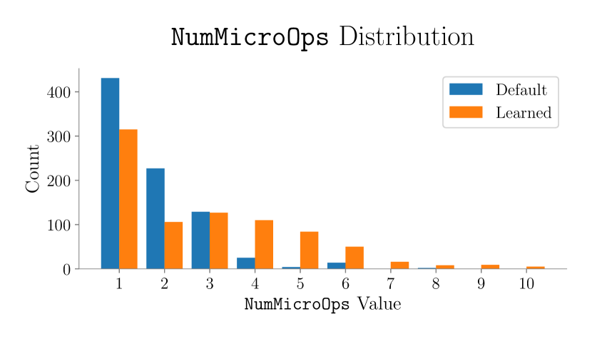
(a) Distribution of default and learned NumMicroOps values.

(b) Distribution of default and learned WriteLatency values.

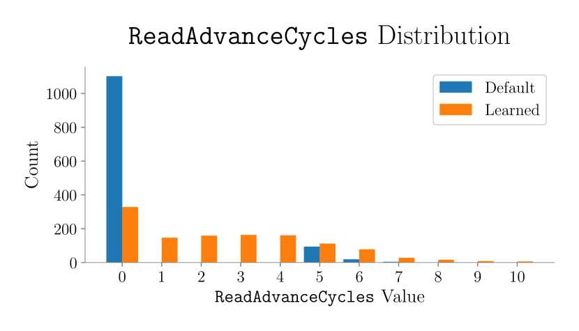
(c) Distribution of default and learned ReadAdvanceCycles values.

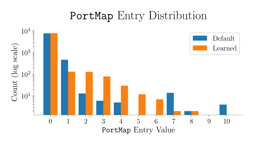
(d) Distribution of default and learned PortMap values.

Figure 4: Distributions of default and learned parameter values on Haswell.

VI Analysis

In this section, we analyze the parameters learned by DiffTune on llvm-mca, answering the following research questions:

• How similar are the learned parameters to the default parameters in llvm-mca? (Section VI-A)

• How optimal are the learned parameters? (Section VI-B)

• How semantically meaningful are the learned parameters? (Section VI-C)

VI-A Comparison of Learned Parameters to Defaults

This section compares the default parameters to the learned parameters (from a single run of DiffTune) in Haswell.

Distributional similarities

To determine the distributional similarity of the learned parameters to the default parameters, Figure 4 shows histograms of the values of the default and learned per-instruction parameters (NumMicroOps, WriteLatency, ReadAdvanceCycles, PortMap). The primary distinctions between the distributions are in WriteLatency and ReadAdvanceCycles; the learned parameters otherwise follow similar distributions to the defaults.

The distributions of default and learned WriteLatency values in Figure 4(b) primarily differ in that only 1 out of the 837 opcodes in the default Haswell parameters has WriteLatency 0 (VZEROUPPER), whereas 251 out of the 837 opcodes in the learned parameters have WriteLatency 0. As discussed in Table II, a WriteLatency value of 0 means that dependent instructions do not have to wait before being issued, and can be issued in the same cycle; instructions may still be bottlenecked elsewhere in the simulation pipeline (e.g., in the execute stage).

The distributions of default and learned ReadAdvanceCycles are presented in Figure 4(c). The default ReadAdvanceCycles are mostly 0, with a small population having values 5 and 7; in contrast, the learned ReadAdvanceCycles are fairly evenly distributed, with a plurality being 0. Given that a significant fraction of learned WriteLatency values are 0, it is likely that many ReadAdvanceCycles values have little to no effect.

TABLE VI: Default and learned global parameters.

Architecture Parameters	DispatchWidth	ReorderBufferSize
Haswell Default	4	192
Learned	4	144

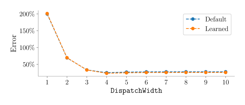
Figure 5: llvm-mca’s sensitivity to values of DispatchWidth (Top) and ReorderBufferSize (Bottom) within the default (Blue) and learned (Orange) parameters.

Global parameters

Table VI shows the default and learned global parameters (DispatchWidth and ReorderBufferSize). The learned DispatchWidth parameter is close to the default DispatchWidth parameter, while the learned ReorderBufferSize parameter differs significantly from the default. By analyzing llvm-mca’s sensitivity to values of DispatchWidth and ReorderBufferSize within the default and learned parameters in Figure 5, we find that although the learned global parameters do not match the default values exactly, they approximately minimize llvm-mca’s error because there is a wide range of values that result in approximately the same error. While llvm-mca is sensitive to small perturbations in the value of the DispatchWidth parameter (with the default parameters, a DispatchWidth of $3$ has error $33.5\%$, $4$ has error $25.0\%$, and $5$ has error $26.8\%$), it is relatively insensitive to perturbations of the ReorderBufferSize (with the default parameters, all ReorderBufferSize values above $70$ have error $25.0\%$). This is primarily because one of llvm-mca’s core modeling assumptions, that memory accesses always resolve in the L1 cache, means that most instructions spend few cycles in the issue, execute, and retire phases; the ReorderBufferSize is therefore rarely a bottleneck in llvm-mca’s modeling of the BHive dataset.

VI-B Optimality

This section shows that while the parameters learned by DiffTune match the error of the default parameters, the learned values are not optimal: by using DiffTune to optimize just a subset of llvm-mca’s parameters, and keeping the rest as their expert-tuned default values, we are able to find parameters with lower error than when learning the entire set of parameters.

Experiment

We learn only each instruction’s WriteLatency in llvm-mca. We keep all other parameters as their default values. The dataset and objective used in this task are otherwise the same as presented in Section V-A.

Methodology

Training hyperparameters are similar to those presented in Section V-A, and are reiterated here with modifications made to learn just WriteLatency parameters. We train both the surrogate and the parameter table using Adam [21] with a batch size of 256. We use a learning rate of $0.001$ to train the surrogate and a learning rate of $0.05$ to train the parameter table. To train the surrogate, we generate a simulated dataset of $2301110$ blocks. For each basic block in the simulated dataset, we sample a random parameter table, with each WriteLatency a uniformly random integer between $0$ and $10$ (inclusive). We loop over this simulated dataset $3$ times when training the surrogate. To train the parameter table, we initialize it to a random sample from the parameter training distribution, then train it for $1$ epoch against the original training set.

Results

On Haswell, this application of DiffTune results in an error of $16.2\%$ and a Kendall Tau correlation coefficient of $0.823$, compared to an error of $23.7\%$ and a correlation of $0.745$ when learning the full set of parameters with DiffTune. These results demonstrate that DiffTune does not find a globally optimal parameter set when learning llvm-mca’s full set of parameters. This suboptimality is due in part to the non-convex nature of the problem and the size of the parameter space.

VI-C Case Studies

This section presents case studies of basic blocks simulated with the default and with the learned parameters, showing where the learned parameters better reflect the ground truth data, and where the learned parameters reflect degenerate cases of the optimization algorithm. To simplify exposition, the results in this section use just the learned WriteLatency values from the experiment in Section VI-B.

PUSH64r

The default WriteLatency with the Haswell parameters for the PUSH64r opcode (push a 64-bit register onto the stack, decrementing the stack pointer) is 2 cycles. In contrast, the WriteLatency learned by DiffTune is 0 cycles. This leads to significantly more accurate predictions for blocks that contain PUSH64r opcodes, such as the following (in which the default and learned latency for testl are both 1 cycle):

⬇

pushq %rbx

testl %r8d, %r8d

The true timing of this block as measured by Chen et al. [23] is 1.01 cycles. On this block, llvm-mca with the default Haswell parameters predicts a timing of 2.03 cycles: The PUSH64r forms a dependency chain with itself, so the default WriteLatency before each PUSH64r can be dispatched is 2 cycles. In contrast, llvm-mca with the learned Haswell values predicts that the timing is 1.03 cycles, because the learned WriteLatency is 0 meaning that there is no delay before the following PUSH64r can be issued, but the PortMap for PUSH64r still occupies HWPort4 for a cycle before the instruction is retired; this 1-cycle dependency chain results in a more accurate prediction. In this case, DiffTune learns a WriteLatency that leads to better accuracy for the PUSH64r opcode.

XOR32rr

The default WriteLatency in Haswell for the XOR32rr opcode (xor two registers with each other) is 1 cycle. The WriteLatency learned by DiffTune is again 0 cycles. This is not always correct – however, a common use of XOR32rr is as a zero idiom, an instruction that sets a register to zero. For example, xorq %rax, %rax performs an xor of %rax with itself, effectively setting %rax to zero. Intel processors have a fast path for zero idioms – rather than actually computing the xor, they simply set the value to zero. Most of the instances of XOR32rr in our dataset ($4047$ out of $4218$) are zero idioms. This leads to more accurate predictions in the general case, as can be seen in the following example:

⬇

xorl %r13d, %r13d

The true timing of this block is 0.31 cycles. With the default WriteLatency value of 1, the Intel x86 simulation model of llvm-mca does not recognize this as a zero idiom and predicts that this block has a timing of 1.03 cycles. With the learned WriteLatency value of 0 and the fact that there are no bottlenecks specified by the PortMap, llvm-mca executes the xors as quickly as possible, bottlenecked only by the NumMicroOps of $1$ and the DispatchWidth of 4. With this change, llvm-mca predicts that this block has a timing of 0.27 cycles, again closer to the ground truth.

ADD32mr

Unfortunately, it is impossible to distinguish between semantically meaningful values that make the simulator more correct, and degenerate values that improve the accuracy of the simulator without adding interpretability. For instance, consider ADD32mr, which adds a register to a value in memory and writes the result back to memory:

⬇

addl %eax, 16(%rsp)

This block has a true timing of 5.97 cycles because it is essentially a chained load, add, then store—with the L1 cache latency being 4 cycles. However, llvm-mca does not recognize the dependency chain this instruction forms with itself, so even with the default Haswell WriteLatency of 7 cycles for ADD32mr, llvm-mca predicts that this block has an overall timing of 1.09 cycles. Our methodology recognizes the need to predict a higher timing, but is fundamentally unable to change a parameter in llvm-mca to enable llvm-mca to recognize the dependency chain (because no such parameter exists). Instead, our methodology learns a degenerately high WriteLatency of 62 for this instruction, allowing llvm-mca to predict an overall timing of 1.64 cycles, closer to the true value. This degenerate value increases the accuracy of llvm-mca without leading to semantically useful WriteLatency parameters. This case study shows that the interpretability of the learned parameters is only as good as the simulation fidelity; when the simulation is a poor approximation to the physical behavior of the CPU, the learned parameters do not correspond to semantically meaningful values.

VII Future Work

DiffTune is an effective technique to learn simulator parameters, as we demonstrate with llvm-mca (Section V) and llvm_sim (Appendix A). However, there are several aspects of DiffTune’s approach that are designed around the fact that llvm-mca and llvm_sim are basic block simulators that are primarily parameterized by ordinal parameters with few constraints between the values of individual parameters. We believe that DiffTune’s overall approach—differentiable surrogates—can be extended to whole program and full system simulators that have richer parameter spaces, such as gem5, by extending a subset of DiffTune’s individual components.

Whole program and full system simulation

DiffTune requires a differentiable surrogate that can learn the simulator’s behavior to high accuracy. Ithemal [22]—the model we use for the surrogate—operates on basic blocks with the assumption that all data accesses resolve in the L1 cache, which is compatible with our evaluation of llvm-mca and llvm_sim (which make the same assumptions). While Ithemal could potentially model whole programs (e.g., branching) and full systems (e.g., cache behavior) with limited modifications, it may require significant extensions to learn such more complex behavior [33, 34].

In addition to the design of the surrogate, training the surrogate would require a new dataset that includes whole programs, along with any other behavior modeled by the simulator being optimized (e.g., memory). Acquiring such a dataset would require extending timing methodologies like BHive [23] to the full scope of target behavior.

Non-ordinal parameters

DiffTune only supports ordinal parameters and does not support categorical or boolean parameters. DiffTune requires a relaxation of discrete parameters to continuous values to perform optimization, along with a method to extract the learned relaxation back into the discrete parameter type (e.g., DiffTune relaxes integers to real numbers, and extracts the learned parameters by rounding back to integers). Supporting categorical and boolean parameters would require designing and evaluating a scheme to represent and extract such parameters within DiffTune. One candidate representation is one-hot encoding, but has not been evaluated in DiffTune.

Dependent parameters

All integers in the range $[1,\infty)$ are valid settings for llvm-mca’s parameters. However, other simulators, such as gem5, have stricter conditions—expressed as assertions in the simulator—on the relationship among different parameters. DiffTune also does not apply when there is a variable number of parameters: we are able to learn the port mappings in a fixed-size PortMap, but do not learn the number of ports in the PortMap, instead fixing it at 10 (the default value for the Haswell microarchitecture). Extending DiffTune to optimize simulators with rich, dynamic constrained relationships between parameters motivates new work in efficient techniques to sample such sets of parameters [35].

Sampling distributions

Extending DiffTune to other simulators also requires defining appropriate sampling distributions for each parameter. While the sampling distributions do not have to directly lead to parameter settings that lead the simulator to have low error (e.g., the sampling distributions defined in Section V-A lead to an average error of llvm-mca on Haswell of $171.4\%\pm 95.7\%$), they do need to contain values that the parameter table estimate may take on during the parameter table optimization phase (because neural networks like our modification of Ithemal are not guaranteed to be able to accurately extrapolate outside of their training distribution). Other approaches to optimizing with learned differentiable surrogates handle this by continuously re-optimizing the surrogate in a region around the current parameter estimate [16], a promising direction that could alleviate the need to hand-specify proper sampling distributions.

VIII Related Work

Simulators are widely used for architecture research to model the interactions of architectural components of a system [1, 2, 4, 5, 6]. Configuring and validating CPU simulators to accurately model systems of interest is a challenging task [23, 36, 37]. We review related techniques for setting CPU simulator parameters in Section VIII-A, as well as related techniques to DiffTune in Section VIII-B.

VIII-A Setting CPU Simulator Parameters

In this section, we discuss related approaches for setting CPU simulator parameters.

Measurement

One methodology for setting the parameters of an abstract model is to gather fine-grained measurements of each individual parameter’s realization in the physical machine [9, 10] and then set the parameters to their measured values [11, 12]. When the semantics of the simulator and the semantics of the measurement methodology coincide, then these measurements can serve as effective parameter values. However, if there is a mismatch between the simulator and measurement methodology, then measurements may not provide effective parameter settings.

All fine-grained measurement frameworks rely on accurate hardware performance counters to measure the parameters of interest. Such performance counters do not always exist, such as with per-port measurement performance counters on AMD Zen [13]. When such performance counters are present, they are not always reliable [38].

Optimizing CPU simulators

Another methodology for setting parameters of an abstract model is to infer the parameters from end-to-end measurements of the performance of the physical machine. In the most related effort in this space, Ritter and Hack [13] present a framework for inferring port usage of instructions based on optimizing against a CPU model that solves a linear program to predict the throughput of a basic block. Their approach is specifically designed to infer port mappings and it is not clear how the approach could be extended to infer different parameters in a more complex simulator, such as extending their simulation model to include data dependencies, dispatch width, or reorder buffer size. To the best of our knowledge, DiffTune is the first approach designed to optimize an arbitrary simulator, provided that the simulator and its parameters match DiffTune’s scope of applicability (Section VII).

VIII-B Differentiable surrogates and approximations

In this section, we survey techniques related to DiffTune that facilitate optimization by using differentiable surrogates or approximations.

Optimization with learned differentiable surrogates

Optimization of black-box and non-differentiable functions with learned differentiable surrogates is an emerging set of techniques, with applications in computer graphics [39], physical sciences [16, 17], reinforcement learning [18], and computer security [19]. Tseng et al. [39] use a convolutional neural network as a learned differentiable surrogate to optimize 32 parameters in a black-box camera imaging pipeline. Shirobokov et al. [16] use learned differentiable surrogates to optimize parameters for generative models of small physics simulators. This technique is similar to an iterative version of DiffTune that continuously re-optimizes the surrogate around the current parameter table estimate. Louppe and Cranmer [17] propose optimizing non-differentiable physics simulators by formulating the joint optimization problem as adversarial variational optimization. Louppe and Cranmer’s technique is applicable in principle, though it has only been evaluated in small settings with a single parameter to learn. Grathwohl et al. [18] use learned differentiable surrogates to approximate the gradient of black-box or non-differentiable functions, in order to reduce the variance of gradient estimators of random variables. While similar, Grathwohl et al.’s surrogate optimization has a different objective: reducing the variance of other gradient estimators [40], rather than necessarily mimicking the black-box function. She et al. [19] use learned differentiable surrogates to approximate the branching behavior of real-world programs then find program inputs that trigger bugs in the program. She et al.’s surrogate does not learn the full input-output behavior of the program, only estimating which edges in the program graph are or are not taken.

CPU simulator surrogates

İpek et al. [41] use neural networks to learn to predict the IPC of a cycle-accurate simulator given a set of design space parameters, to enable efficient design space exploration. Lee and Brooks [42] use regression models to predict the performance and power usage of a CPU simulator, similarly enabling efficient design space exploration. Neither İpek et al. nor Lee and Brooks then use the models to optimize the simulator to be more accurate; both also apply exhaustive or grid search to explore the parameter space, rather than using the gradient of the simulator surrogate.

Differentiating arbitrary programs

Chaudhuri and Solar-Lezama [43] present a method to approximate numerical programs by executing programs probabilistically, similar to the idea of blurring an image. This approach lets Chaudhuri and Solar-Lezama apply gradient descent to parameters of arbitrary numerical programs. However, the semantics presented by Chaudhuri and Solar-Lezama only apply to a limited set of program constructs and do not easily extend to the set of program constructs exhibited by large-scale CPU simulators.

TABLE VII: Parameters learned for llvm_sim.

Parameter	Count	Constraint	Description
WriteLatency	1 per-instruction	Integer, $\geq 0$	The number of cycles before destination operands of that instruction can be read from.
PortMap	10 per-instruction	Integer, $\geq 0$	The number of micro-ops dispatched to each port.

TABLE VIII: Learning all parameters: error of llvm_sim with the default and learned parameters.

Architecture Predictor	Error	Kendall’s Tau
Haswell Default	$61.3\%$	0.7256
DiffTune	$44.1\%$	0.718
Ithemal	$9.2\%$	0.854
IACA	$17.1\%$	0.800
OpenTuner	$115.6\%$	0.507

IX Conclusion

CPU simulators are complex software artifacts that require significant measurement and manual tuning to set their parameters. We present DiffTune, a generic algorithm for learning parameters within non-differentiable programs, using only end-to-end supervision. Our results demonstrate that DiffTune is able to learn the entire set of 11265 microarchitecture-specific parameters from scratch in llvm-mca. Looking beyond CPU simulation, DiffTune’s approach offers the promise of a generic, scalable methodology to learn the parameters of programs using only input-output examples, potentially reducing many programming tasks to simply that of gathering data.

Appendix A llvm_sim

To evaluate that our implementation of DiffTune (Section IV) is extensible to simulators other than llvm-mca, we evaluate our implementation on llvm_sim [7], learning all parameters that llvm_sim reads from LLVM. llvm_sim is a simulator that uses many of the same parameters (from LLVM’s backend) as llvm-mca, but uses a different model of the CPU, modeling the frontend and breaking up instructions into micro-ops and simulating the micro-ops individually rather than simulating instructions as a whole as llvm-mca does.

Behavior

llvm_sim [7] is also an out-of-order superscalar simulator exposing LLVM’s instruction scheduling model. llvm_sim is only implemented for the x86 Haswell microarchitecture. Similar to llvm-mca, llvm_sim also predicts timings of basic blocks, assuming that all data is in the L1 cache. llvm_sim primarily differs from llvm-mca in two aspects: It models the front-end, and it decodes instructions into micro-ops before dispatch and execution. llvm_sim has the following pipeline:

• Instructions are fetched, parsed, and decoded into micro-ops (unlike llvm-mca, llvm_sim does model the frontend)

• Registers are renamed, with an unlimited number of physical registers

• Micro-ops are dispatched out-of-order once dependencies are available

• Micro-ops are executed on execution ports

• Instructions are retired once all micro-ops in an instruction have been executed

Parameters

We learn the parameters specified in Table VII. We again assume that there are 10 execution ports available to dispatch for all microarchitectures and do not learn to dispatch to port groups. All other hyperparameters are identical to those described in Section V-A.

Results

Table VIII presents the average error and correlation of llvm_sim with the default parameters, llvm_sim with the learned parameters, Ithemal trained on the dataset as a lower bound, and the OpenTuner [14] baseline. By learning the parameters that llvm_sim reads from LLVM, we reduce llvm_sim’s error from $61.3\%$ to $44.1\%$.

References

- Binkert et al. [2011] N. Binkert, B. Beckmann, G. Black, S. K. Reinhardt, A. Saidi, A. Basu, J. Hestness, D. R. Hower, T. Krishna, S. Sardashti, R. Sen, K. Sewell, M. Shoaib, N. Vaish, M. D. Hill, and D. A. Wood, “The gem5 simulator,” SIGARCH Computer Architecture News, vol. 39, no. 2, 2011.
- Di Biagio and Davis [2018] A. Di Biagio and M. Davis. (2018) llvm-mca. [Online]. Available: https://lists.llvm.org/pipermail/llvm-dev/2018-March/121490.html
- Intel [2017] Intel. (2017) Intel architecture code analyzer. [Online]. Available: https://software.intel.com/en-us/articles/intel-architecture-code-analyzer
- Yourst [2007] M. T. Yourst, “PTLsim: A cycle accurate full system x86-64 microarchitectural simulator,” in IEEE International Symposium on Performance Analysis of Systems Software, 2007.
- Patel et al. [2011] A. Patel, F. Afram, S. Chen, and K. Ghose, “MARSS: A full system simulator for multicore x86 cpus,” in ACM/EDAC/IEEE Design Automation Conference, 2011.
- Sanchez and Kozyrakis [2013] D. Sanchez and C. Kozyrakis, “Zsim: Fast and accurate microarchitectural simulation of thousand-core systems,” in International Symposium on Computer Architecture, 2013.
- Sykora et al. [2018] O. Sykora, C. Courbet, G. Chatelet, and N. Paglieri. (2018) EXEgesis Project. [Online]. Available: https://github.com/google/EXEgesis
- Patterson and Hennessy [1990] D. A. Patterson and J. L. Hennessy, Computer Architecture: A Quantitative Approach. Morgan Kaufmann Publishers Inc., 1990.
- Fog [1996] A. Fog, “Instruction tables: Lists of instruction latencies, throughputs and micro-operation breakdowns for Intel, AMD and VIA CPUs,” Technical University of Denmark, Tech. Rep., 1996.
- Abel and Reineke [2019] A. Abel and J. Reineke, “uops.info: Characterizing latency, throughput, and port usage of instructions on Intel microarchitectures,” in International Conference on Architectural Support for Programming Languages and Operating Systems, 2019.
- Colombet [2014] Q. Colombet. (2014) [patch][x86][haswell][schedmodel] add exceptions for instructions that diverge from the generic model. [Online]. Available: https://lists.llvm.org/pipermail/llvm-commits/Week-of-Mon-20140811/230499.html
- Topper [2014] C. Topper. (2014) [patch] d73844: [x86] update the haswell and broadwell scheduler information for gather instructions. [Online]. Available: https://lists.llvm.org/pipermail/llvm-commits/Week-of-Mon-20200127/738394.html
- Ritter and Hack [2020] F. Ritter and S. Hack, “PMEvo: Portable inference of port mappings for out-of-order processors by evolutionary optimization,” in ACM SIGPLAN Conference on Programming Language Design and Implementation, 2020.
- Ansel et al. [2014] J. Ansel, S. Kamil, K. Veeramachaneni, J. Ragan-Kelley, J. Bosboom, U.-M. O’Reilly, and S. Amarasinghe, “OpenTuner: An extensible framework for program autotuning,” in International Conference on Parallel Architectures and Compilation Techniques, 2014.
- Queipo et al. [2005] N. V. Queipo, R. T. Haftka, W. Shyy, T. Goel, R. Vaidyanathan, and P. Kevin Tucker, “Surrogate-based analysis and optimization,” Progress in Aerospace Sciences, vol. 41, no. 1, 2005.
- Shirobokov et al. [2020] S. Shirobokov, V. Belavin, M. Kagan, A. Ustyuzhanin, and A. G. Baydin, “Black-box optimization with local generative surrogates,” in Workshop on Real World Experiment Design and Active Learning at International Conference on Machine Learning, 2020.
- Louppe and Cranmer [2019] G. Louppe and K. Cranmer, “Adversarial variational optimization of non-differentiable simulators,” in International Conference on Artificial Intelligence and Statistics, 2019.
- Grathwohl et al. [2018] W. Grathwohl, D. Choi, Y. Wu, G. Roeder, and D. Duvenaud, “Backpropagation through the void: Optimizing control variates for black-box gradient estimation,” in International Conference on Learning Representations, 2018.
- She et al. [2019] D. She, K. Pei, D. Epstein, J. Yang, B. Ray, and S. Jana, “NEUZZ: Efficient fuzzing with neural program smoothing,” IEEE Symposium on Security and Privacy, 2019.
- Robbins and Monro [1951] H. Robbins and S. Monro, “A stochastic approximation method,” Annals of Mathematical Statistics, vol. 22, no. 3, 1951.
- Kingma and Ba [2015] D. P. Kingma and J. Ba, “Adam: A method for stochastic optimization,” in International Conference on Learning Representations, 2015.
- Mendis et al. [2019] C. Mendis, A. Renda, S. Amarasinghe, and M. Carbin, “Ithemal: Accurate, portable and fast basic block throughput estimation using deep neural networks,” in International Conference on Machine Learning, 2019.
- Chen et al. [2019] Y. Chen, A. Brahmakshatriya, C. Mendis, A. Renda, E. Atkinson, O. Sykora, S. Amarasinghe, and M. Carbin, “BHive: A benchmark suite and measurement framework for validating x86-64 basic block performance models,” in IEEE International Symposium on Workload Characterization, 2019.
- Laukemann et al. [2018] J. Laukemann, J. Hammer, J. Hofmann, G. Hager, and G. Wellein, “Automated instruction stream throughput prediction for intel and amd microarchitectures,” in IEEE/ACM International Workshop on Performance Modeling, Benchmarking and Simulation of High Performance Computer Systems, 2018.
- Lattner and Adve [2004] C. Lattner and V. Adve, “LLVM: A compilation framework for lifelong program analysis & transformation,” in International Symposium on Code Generation and Optimization, 2004.
- Pohl et al. [2020] A. Pohl, B. Cosenza, and B. Juurlink, “Vectorization cost modeling for NEON, AVX and SVE,” Performance Evaluation, vol. 140-141, 2020.
- Mendis and Amarasinghe [2018] C. Mendis and S. Amarasinghe, “GoSLP: Globally optimized superword level parallelism framework,” ACM International Conference on Object Oriented Programming Systems Languages and Applications, 2018.
- [28] “Intel 64 and IA-32 Architectures Software Developer’s Manual,” https://software.intel.com/en-us/articles/intel-sdm.
- Topper [2018] C. Topper. (2018) Patch] d44644: [x86] use silvermont cost model overrides for goldmont as well. [Online]. Available: http://lists.llvm.org/pipermail/llvm-commits/Week-of-Mon-20180319/537000.html
- Hochreiter and Schmidhuber [1997] S. Hochreiter and J. Schmidhuber, “Long short-term memory,” Neural Computation, vol. 9, no. 8, 1997.
- Hermans and Schrauwen [2013] M. Hermans and B. Schrauwen, “Training and analysing deep recurrent neural networks,” in Advances in Neural Information Processing Systems, 2013.
- Di Biagio [2020] A. Di Biagio, “[llvm-dev] [llvm-mca] resource consumption of procresgroups,” http://lists.llvm.org/pipermail/llvm-dev/2020-May/141486.html, 2020.
- Vila et al. [2020] P. Vila, P. Ganty, M. Guarnieri, and B. Köpf, “Cachequery: Learning replacement policies from hardware caches,” in ACM SIGPLAN Conference on Programming Language Design and Implementation, 2020.
- Hashemi et al. [2018] M. Hashemi, K. Swersky, J. A. Smith, G. Ayers, H. Litz, J. Chang, C. Kozyrakis, and P. Ranganathan, “Learning memory access patterns,” in International Conference on Machine Learning, 2018.
- Dutra et al. [2018] R. Dutra, K. Laeufer, J. Bachrach, and K. Sen, “Efficient sampling of SAT solutions for testing,” in International Conference on Software Engineering, 2018.
- Gutierrez et al. [2014] A. Gutierrez, J. Pusdesris, R. G. Dreslinski, T. N. Mudge, C. Sudanthi, C. D. Emmons, M. Hayenga, and N. C. Paver, “Sources of error in full-system simulation,” IEEE International Symposium on Performance Analysis of Systems and Software, 2014.
- Akram and Sawalha [2019] A. Akram and L. Sawalha, “Validation of the gem5 simulator for x86 architectures,” in IEEE International Workshop on Performance Modeling, Benchmarking and Simulation of High Performance Computer Systems, 2019.
- Weaver and McKee [2008] V. M. Weaver and S. A. McKee, “Can hardware performance counters be trusted?” in IEEE International Symposium on Workload Characterization, 2008.
- Tseng et al. [2019] E. Tseng, F. Yu, Y. Yang, F. Mannan, K. S. Arnaud, D. Nowrouzezahrai, J.-F. Lalonde, and F. Heide, “Hyperparameter optimization in black-box image processing using differentiable proxies,” ACM Transactions on Graphics, no. 4, 7 2019.
- Williams [1992] R. J. Williams, “Simple statistical gradient-following algorithms for connectionist reinforcement learning,” Machine Learning, vol. 8, no. 3-4, 1992.
- İpek et al. [2006] E. İpek, S. A. McKee, R. Caruana, B. R. de Supinski, and M. Schulz, “Efficiently exploring architectural design spaces via predictive modeling,” in International Conference on Architectural Support for Programming Languages and Operating Systems, 2006.
- Lee and Brooks [2007] B. C. Lee and D. M. Brooks, “Illustrative design space studies with microarchitectural regression models,” in IEEE International Symposium on High Performance Computer Architecture, 2007.