Spatially-Variant CNN-based Point Spread Function Estimation for Blind Deconvolution and Depth Estimation in Optical Microscopy

Abstract

Optical microscopy is an essential tool in biology and medicine. Imaging thin, yet non-flat objects in a single shot (without relying on more sophisticated sectioning setups) remains challenging as the shallow depth of field that comes with high-resolution microscopes leads to unsharp image regions and makes depth localization and quantitative image interpretation difficult.

Here, we present a method that improves the resolution of light microscopy images of such objects by locally estimating image distortion while jointly estimating object distance to the focal plane. Specifically, we estimate the parameters of a spatially-variant Point Spread Function (PSF) model using a Convolutional Neural Network (CNN), which does not require instrument- or object-specific calibration. Our method recovers PSF parameters from the image itself with up to a squared Pearson correlation coefficient of 0.99 in ideal conditions, while remaining robust to object rotation, illumination variations, or photon noise. When the recovered PSFs are used with a spatially-variant and regularized Richardson-Lucy (RL) deconvolution algorithm, we observed up to 2.1 dB better Signal-to-Noise Ratio (SNR) compared to other Blind Deconvolution (BD) techniques. Following microscope-specific calibration, we further demonstrate that the recovered PSF model parameters permit estimating surface depth with a precision of 2 micrometers and over an extended range when using engineered PSFs. Our method opens up multiple possibilities for enhancing images of non-flat objects with minimal need for a priori knowledge about the optical setup.

I Introduction

Researchers and physicians intensively use optical microscopes to observe and quantify cellular function, organ development, or disease mechanisms. Despite the availability of many volumetric imaging methods (in particular, optical sectioning methods), single-shot wide-field microscopy remains an important tool to image small and relatively shallow objects. However, non-flat areas, which are out of focus, lead to unsharp regions in the image, making localization and visual interpretation difficult. Image formation in a microscope can be modeled by light diffraction, which causes sharp point-like objects to appear blurry [1]. Because the optical system only collects a fraction of the light emanating from a point on the object, it cannot focus the light into a perfect point and, instead, spreads the light into a three-dimensional diffraction pattern described by the Point Spread Function (PSF). As the image is formed by superposing the contribution of all points in the object, knowledge of the local diffraction pattern, which sums up the optical system and its aberrations, can be used to estimate a sharper image [2].

For thin, yet not flat samples, image formation can be modeled as a superposition of 2D PSFs. These are shaped both by the optical system and the three-dimensional depth of the object. Knowledge of the local PSF could therefore both be used to recover the image and estimate its depth, which usually requires careful camera calibration and ad-hoc focus estimation [3], acquisition of focal depth stacks ([4, 5]), or coherent imaging, such as digital holographic microscopy [6], to numerically refocus the image. Using an adequate PSF, i.e. one that corresponds to the blur, in a deconvolution algorithm can restore details in the image [7]. PSF estimation can be achieved by many techniques [8], but most of them are either dependent on a tedious calibration step, such as the experimental measurement of the PSF, or are sensitive to noise or image variability. Blind Deconvolution (BD) techniques are methods able to recover features in the image without prior knowledge of the PSF.

Here, we aim at estimating the local PSF only from the acquired image and use it to reverse the local degradation due to the optical system. Furthermore, we aim at estimating the depth of any location on the surface of a thin object with respect to the focal plane. We rely on a model-based approach that retrieves the PSF given a degraded image patch via a machine learning approach.
Machine learning technologies have improved our ability to classify images [9], detect objects [10], describe content [11], and estimate image quality [12]. Convolutional Neural Networks (CNNs), in particular, have the ability to learn correlations between an image input and a defined outcome and appear well adapted to determining the degradation kernel directly from the image texture. A similar reasoning led to recent results by Zhu et al. [13], Sun et al. [14], Gong et al. [15] and Nah et al. [16], where the direction and amplitude of motion blur was determined by a CNN classifier from images blurred with a Gaussian kernel. Our approach is similar to that of [14] but with PSF models that are tailored to the specificities of microscopy, a concept that we initially introduced in [17] and that has since been used by other groups such as [18]. In particular, we considered a more generic physical model that can accommodate large-support PSFs. CNNs were also used in a end-to-end manner to enhance details in biological images by performing supervised interpolation [19, 20, 21] or to emulate confocal stacks of sparse 3D structures from widefield images [22].
In this paper, we propose a method to:

1. Find the spatially-variant PSF of the degraded image of a thin, non-flat object directly from the image texture without any instrument-specific calibration step. The PSF determination technique is derived from the one we proposed in [17], which recovers local Zernike moments of the PSF. We focus here on improving the degradation model and quantitatively assess the robustness of the method.

2. Deconvolve the image in a blind and spatially-variant manner, using a regularized Richardson-Lucy algorithm with an overlap-add approach.

3. Extract the depth of a three-dimensional surface from a single two-dimensional image using combinations of Zernike moments.

This technique allows us to enhance the acquired image and recover the three-dimensional structure of a two-dimensional manifold in a 3D space using a single 2D image as an input.

This paper is organized as follows. In Section II, we present the method, comprising the image formation model, the degradation model, the data set generation process, the different neural networks to be trained, the PSF mapping, the deconvolution algorithm, and the depth from focus algorithm. Then, in Section III, we characterize the regression performance of the CNN for different modalities, as well as the gain in resolution from the deconvolution, and the precision of depth detection. We then discuss our findings in Section IV and conclude in Section V.

II Methods

II-A Object and image formation model

We consider a two-dimensional manifold in 3D-space with local intensity $x(\bm{r})$, e.g. an infinitely thin sample suspended in a gel, which can be parameterized by the lateral coordinates $\bm{r}=(r_{1},r_{2})$ and axial coordinate $z(\bm{r})$. We express the resulting three-dimensional object as:

$$x_{3D}(\bm{r},r_{3})=x(\bm{r})\delta(r_{3}-z(\bm{r})),$$ (1)

where $(\bm{r},r_{3})=(r_{1},r_{2},r_{3})$ are coordinates in 3D object space. We further consider an optical imaging system with camera coordinates $\bm{s}=(s_{1},s_{2})$ and axial position $s_{3}$, characterized by a spatially-varying point spread function $h_{\text{3D}}(\bm{s},s_{3},\bm{r},r_{3})$ (see Fig. 1). For a fixed axial camera position $s_{3}$, the measured intensity by a pixel at position $\bm{s}$ is given by the convolution (Fig. 1 (a)) [23]:

$$y_{\text{3D}}(\bm{s},s_{3})=\iiint x_{\text{3D}}(\bm{r},r_{3})h_{\text{3D}}(\bm{s},s_{3},\bm{r},r_{3})\text{d}\bm{r}\text{d}r_{3},$$ (2)

where we assumed, to simplify the notation, that the magnification is 1. When the microscope is focused at the origin ($s_{3}=0$) we define the 2D image $y(\bm{s})=y_{\text{3D}}(\bm{s},s_{3})\bigr{|}_{s_{3}=0}$, which can be obtained via the expression:

$$y(\bm{s}) =\iiint x(\bm{r})\delta(r_{3}-z(\bm{r}))h_{\text{3D}}(\bm{s},s_{3}=0,\bm{r},r_{3})\text{d}\bm{r}\text{d}r_{3}$$ (3)

$$=\iint x(\bm{r})h_{\text{3D}}(\bm{s},s_{3}=0,\bm{r},r_{3}=z(\bm{r}))\text{d}\bm{r}$$ (4)

$$=\iint x(\bm{r})h(\bm{s},\bm{r})\text{d}\bm{r},$$ (5)

where $h(\bm{s},\bm{r})=h_{\text{3D}}(\bm{s},s_{3}=0,\bm{r},r_{3}=z(\bm{r}))$ is a 2D point spread function that incorporates both the local (3D) variations of the optical system and the variable depth of the thin sample. We further assume that $h(\bm{s},\bm{r})$ can be approximated by a parametric function $\widetilde{h}_{\bm{a}(\bm{s})}(\bm{r})$, where the $N$ parameters $\bm{a}(\bm{s})=\begin{matrix}(a_{1}(\bm{s})&a_{2}(\bm{s})&\cdots&a_{N}(\bm{s}))\end{matrix}$ can vary for every 2D location $\bm{s}$ of the image (Fig. 1 (b)).

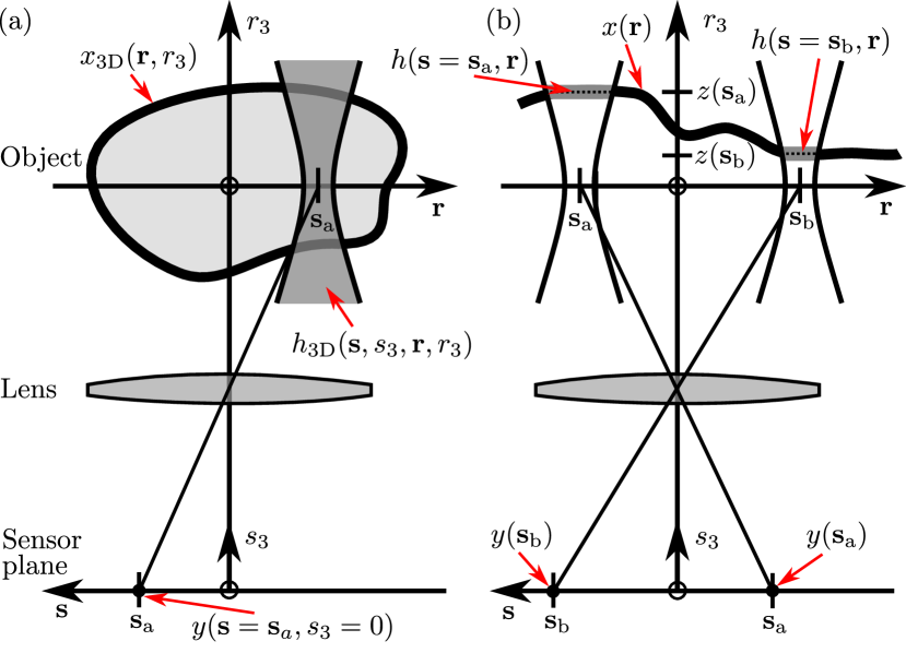
Figure 1: Object and image formation model. (a) General thick 3D object case, (b) Approximate manifold case.

II-B Parametric degradation models

There are many methods for estimating the PSF of a degraded image. Such methods can be categorized into two classes: direct PSF estimation or parametric modeling. In works such as those by Grossmann et al. [3], the PSFs are estimated directly from the image (e.g. using edge detection and a regression model [24], a Maximum a Posteriori (MAP) prediction [25]), or via a camera calibration using images of a defined and known pattern [26] [27]. Levin et al. [28] showed that a MAP approach to recover the blur kernel is well constrained, but that the MAP global optimum for the recovered image is a blurred image because the strong constraints do not always generalize to unexpected or noisy types of data [29], which are common in microscopy images. Full pixel-wise PSFs can also be estimated using dictionary learning [30], or CNNs [31]. However, this latter kind of estimation is not well constrained and can generate over-fitting artifacts.

In contrast, parametric modeling of the PSF allows to reduce the dimensionality of the optimization problem and to attach a physical meaning to the parameters, such as the relative distance from the focal point, or optical aberrations such as astigmatism. There are many mathematical models to represent the PSF of a microscope. They can take into account both physical characteristics of the objectives (for example numerical aperture, correction types, etc.) and of the experimental conditions (focal distance and immersion medium) [32]. In many cases, the model parameters correspond to physical design conditions, such as optical distances, aperture diameters, or foci. A simple PSF model can be obtained from the Fraunhofer diffraction theory to calculate the diffraction of a circular aperture [33]. The Gibson & Lanni model accounts for the immersion medium, the cover-slip, the sample layers, different medium numerical apertures, and the properties of the objective [1]. Despite their theoretical relevance, in practice, numerical values for these parameters may not be available, as detailed information about all experimental and design conditions may be lacking. Even if the parameters are accessible, they may be missing if they were not recorded along with the image.

Since we aim to recover the PSF from the image itself, with minimal knowledge of the imaging conditions, we focused on models specified by only a small number of parameters or whose complexity can be adjusted progressively by considering approximations with a subset of the complete set of parameters. Specifically, we considered PSF models based on Zernike polynomials, which are used to describe the wavefront function of lenses such as the eye [34], as well as anisotropic Gaussian models.

II-B1 Zernike polynomial decomposition of the pupil function

Optical abnormalities, such as de-focus, astigmatism, or spherical aberrations, can be modeled with a superposition of Zernike polynomials $Z_{n}(\bm{\xi})$ in the expansion of the microscope objective’s pupil function $W_{\bm{a}(\bm{s})}$ [35]:

$$W_{\bm{a}(\bm{s})}(\bm{\xi})=\sum_{n=1}^{N}Z_{n}(\bm{\xi},a_{n}(\bm{s})),$$ (6)

where $\bm{\xi}$ denotes the two-vector of spatial coordinates in the pupil plane perpendicular to the optical axis, $N$ the maximal order of considered aberrations, and $a_{n}(\bm{s})$ the parameter corresponding to each Zernike term $Z_{n}$. In our experiments, $Z_{1}$ describes the de-focus term, $Z_{2}$ describes the power of the astigmatism (cylinder), and $Z_{3}$ describes the astigmatism angle (axis). The pupil function can ultimately be converted into a PSF [36]:

$$\widetilde{h}_{\bm{a}(\bm{s})}(\bm{r})\propto\left|\mathcal{F}\left\{W_{\bm{a}(\bm{s})}\left(\frac{\bm{r}}{\lambda}\right)\right\}\right|^{2},$$ (7)

with $\mathcal{F}$ the Fourier transform and $\lambda$ the wavelength of the light.

II-B2 Anisotropic Gaussian model

For many applications, Gaussian distributions are sufficiently accurate approximations of the diffraction-limited PSF of wide field microscopes [37]. We extend the model by allowing for anisotropy, which we require to describe astigmatic aberrations, or if the spatial resolution in one lateral direction is different from that in the other. The detection method is in that case similar to the one described in [14]. The PSF is then defined by the anisotropic zero-centered normal probability density function:

$$\widetilde{h}_{\bm{a}(\bm{s})}(\bm{r})=\frac{1}{\sqrt{2\pi a_{1}(\bm{s})}}\exp\left({-\frac{1}{2}\frac{{r_{1}}^{2}}{a_{1}(\bm{s})}}\right)\\ \cdot\frac{1}{\sqrt{2\pi a_{2}(\bm{s})}}\exp\left({-\frac{1}{2}\frac{{r_{2}}^{2}}{a_{2}(\bm{s})}}\right),$$ (8)

where $a_{1}$ and $a_{2}$ are the variances of the Gaussian in the x and y axes, respectively.

II-C Problem statement

We aim to solve several problems. First, given only an observed degraded image $y(\bm{s})$, we want to estimate the PSF model $\widetilde{h}_{\bm{a}(\bm{s})}(\bm{r})$ closest to the effective PSF of the imaging system $h(\bm{s},\bm{r})$ for any point $\bm{s}$ without requiring additional information on the microscope or any further calibration images acquired with that microscope. Specifically, we want to infer the model parameters $\bm{a}(\bm{s})$, first locally, then globally. Next, given the local PSF parameters $\bm{a}(\bm{s})$ and the blurred image $y(\bm{s})$, we want to recover an estimate of the non-degraded image $x(\bm{r})$. Finally, we want to infer the local depth $z(\bm{r})$ along the axis of the object at any position $\bm{r}$ in the plane perpendicular to the optical axis thereby allowing us to build $x_{\text{3D}}(\bm{r},z(\bm{r}))$.

II-D Method overview

For each of the problems, we summarize the following main steps:

1. Shift-invariant PSF parameter estimation given an image patch (see Section II-E2)

   1. Select a parametric degradation model for $h_{\bm{a}}(\bm{r})$ allowing the generation of PSF/parameters pairs.

   2. Gather a training library of microscopy images, degrade each image via a spatially-invariant convolution with its corresponding PSF, corrupt it with synthetic noise.

   3. Train a CNN that takes a degraded image patch as input and returns the corresponding degradation model parameters, via regression.

2. Local PSF estimation given a full degraded microscopy image (see Section II-F)

   1. Given a full microscopy image as input, locally extract a patch, then regress the PSF parameters using the steps above.

   2. Repeat in all regions of the image.

   3. Combine the estimated PSF parameters to generate the map $\bm{a}(\bm{s})$ of the local PSF model parameters.

3. Application 1: spatially-variant blind deconvolution (see Section II-G)

   1. Given an input image and the map of estimated local PSF parameters, generate local PSFs $\widetilde{h}_{\bm{a}(\bm{s})}(\bm{r})$.

   2. Use the generated PSFs in a Total Variation regularized Richardson-Lucy (TV-RL) deconvolution algorithm to recover an estimate for $x(\bm{r})$.

4. Application 2: estimate depth from focus using PSF engineering (see Section II-H))

   1. Given an image acquired with a PSF-engineered optical system $y(\bm{s})$ [38]), deduce the depth map $z(\bm{r})$ from the local parameters $\bm{a}(\bm{s})$.

   2. Generate $x_{\text{3D}}(\bm{r},z(\bm{r}))$.

In the following subsections, we provide details on each of these steps.

II-E PSF parameter estimation in image patches (shift-invariant image formation model)

II-E1 Data set generation for CNN training

Given an image patch as input, we wish to estimate the degradation model parameters corresponding to the spatially-invariant PSF that degraded the patch. Since neural networks are trained by adjusting their internal weights using backpropagation of the derivative of a loss function between the ground truth of the training data and the output of the network [39], we establish a training set $T$ (Fig. 2). For that purpose, we gather input images $x^{(k)}$. Since reliable public image data sets have limited size, we augment the size of the training sets by rotating each image by an angle of $\pm 90^{\circ}$, so we have $K$ images, $x^{(k)}$, $k=0,...,K-1$.. We induce a synthetic degradation by convolving the images with $K$ generated PSFs $h_{\bm{a}^{(k)}}$ of model parameters $\bm{a}^{(k)}$ drawn from a normalized and scaled uniform distribution:

$$\psi^{(k)}(\bm{s})=(h_{\bm{a}^{(k)}}\ast x^{(k)})(\bm{s}).$$ (9)

We also consider the two predominant sources of noise in digital image acquisition: the stochastic nature of the quantum effects of the photoconversion process and the intrinsic thermal and electronic fluctuations in the CCD camera [40]. The first source of noise comes from physical constraints such as a low-power light source or short exposure time, while the second is signal-independent. This motivates the noise model as a mixed Gaussian-Poisson noise process. Therefore, we define noise with the two following components:

• A random variable $n_{p}(\bm{s})\sim\mathcal{P}(\lambda=\psi^{(k)}(\bm{s}))$ following a Poisson distribution of probability $P\{n_{p}(\bm{s})=i\}=e^{-\lambda}\lambda^{i}/{i!}$.

• A random variable $b(\bm{s})\sim\mathcal{N}(0,\sigma^{2})$ following a Gaussian distribution with zero-mean and variance $\sigma^{2}$.

The image noise model for data set generation is then:

$$\psi_{\text{noisy}}^{(k)}(\bm{s})=\beta n_{p}(\bm{s})+b(\bm{s}),$$ (10)

with $\beta$ a number between 0 and 1 reflecting the quantum efficiency of the CCD [41]. Images that did not comply with a minimal variance and white pixel ratio were tagged as invalid, i.e. $a^{(k)}_{0}=1$ (see Section II-E2).

We cropped the images $\psi_{\text{noisy}}^{(k)}(\bm{s})$ to a size $K_{\psi}\times L_{\psi}$ by randomly selecting the position of a region of interest of that size. We then paired these image patches with their respective PSF parameter vector $\bm{a}^{(k)}$ in order to form the training set $T=\{(\psi_{\text{noisy}}^{(k)}(\bm{s}),\bm{a}^{(k)})\}_{k=0}^{K-1}$.

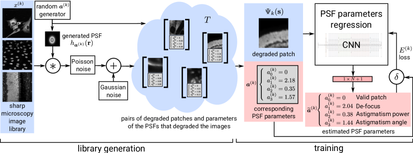
Figure 2: Data set gathering (left) and CNN training (right) pipelines. From a large library of sharp microscopy images, small patches are created, blurred with a PSF generated from random parameters, and degraded with a Poisson-Gaussian noise mixture (see Section II-E1). The resulting patches and the parameters are stored in the training set $T$, that is used for training the CNN. Using backpropagation of the loss function, the CNN output is trained towards the prediction of the PSF model parameters (Section II-E2).

II-E2 CNN training modalities

We considered several neural networks (whose architectures we further describe below) and trained them to learn the PSF model parameters described in Section II-B. The task of the network is to estimate, only from the $k^{\text{th}}$ input image patch $\Psi^{(k)}(\bm{s})$, the parameters $\widetilde{\bm{a}}^{(k)}(\bm{s})$ that have been used by the PSF model to degrade that input image. Since there are cases where the PSF estimation is not possible, e.g. where the sample lacks texture, such as in uniformly black or grey areas, we added a boolean parameter $a^{(k)}_{0}$ (whose values can be either $0$ or $1$), which indicates the legitimacy of the sample. The total number of estimated parameters is then $N+1$. We aim at minimizing the distance between the output of the network $\widetilde{\bm{a}}^{(k)}$ and the ground-truth PSF parameters ${\bm{a}^{(k)}}$. Therefore, in the training phase, we updated the weights of the CNN using the modified Euclidean loss function:

$$E^{(k)}=\gamma\left({a^{(k)}_{0}}-{\widetilde{a}^{(k)}_{0}}\right)^{2}+\frac{1-{a^{(k)}_{0}}}{2N}\sum_{n=1}^{N}({a^{(k)}_{n}}-{\widetilde{a}^{(k)}_{n}})^{2},$$ (11)

with $\gamma$ a hyperparameter regulating the importance of the validity parameter, that we set to $1$ in our further experiments.

We choose to rely on networks that showed good performance in the ImageNet competition, which is a benchmark in object classification on hundreds of categories [42, 43]. Donahue et al. [44] showed that deep convolutional representations can be applied to a variety of tasks and detection of visual features, which drove our selection for estimating optical aberrations. Hendrycks et al. [45] extensively discussed whether the networks were robust to changes in input illumination, noise, and blur. While residual networks that use skip-connections such as ResNet [46] appear to be more robust to input noise than primitive feedforward networks such as AlexNet [9], their performance appears to be surpassed by newer multibranch models such as ResNeXt [47] or Densenet [48]. In the context of our specific task, we compared the performance (see Section III-B) and the robustness to degradation (see Section III-C) of several of the above architectures.

After training, the networks can regress the spatially-invariant PSF parameters $\widetilde{\bm{a}}^{(k)}(\bm{s})$ from a single input image patch $\Psi^{(k)}(\bm{s})$.

II-F Spatially-variant PSF parameter mapping

Given a trained CNN that is able to recover the degradation parameters from a single image patch, we now turn to the problem of locally estimating the parameters of the different PSFs that degraded a larger input image. To achieve this, we use an overlapping sliding window over the input image $x(\bm{r})$ with stride $t$ that is fed into the locally invariant regression CNN trained in Section II-E2 (see Fig. 3). We store the resulting parameters in the map $\widetilde{\bm{A}}=\begin{matrix}(\widetilde{\bm{a}}^{(0)}&\widetilde{\bm{a}}^{(1)}&...&\widetilde{\bm{a}}^{(M)})\end{matrix}$, where $\widetilde{\bm{a}}^{(m)}$ is the output of the neural network for patch $m$ and $M$ is the total number of patches. Using the PSF model, we generate from $\widetilde{\bm{A}}$ a spatially-variant map of local PSF kernels defined as $\widetilde{{H}}=\begin{matrix}(\widetilde{{h}}^{(0)}(r)&\widetilde{{h}}^{(1)}(r)&\cdots&\widetilde{{h}}^{(M)}(r))\end{matrix}$.
The overlapping window over the input image yields a map of $\left(\lfloor({K_{x}-K_{\psi}})/t\rfloor+1\right)\times\left(\lfloor({L_{x}-L_{\psi}})/t\rfloor+1\right)$ kernels, with $K_{x}$, $L_{x}$, and $K_{\psi}$, $L_{\psi}$ being the width and height of the input image and the window step size, respectively. For example, a $1024\times 1024$ pixel input image using $128\times 128$ pixel patches and $t=64$ yields $M=13\times 13$ spatially-dependent PSF kernels. We fill every patch with a validity parameter $a_{0}=1$ (i.e. invalid) with the content of the inverse Euclidean distance-weighted average of the four-connected nearest neighbors using K-Nearest Neighbor regression [49] in order to avoid boxing artifacts during the later deconvolution process.

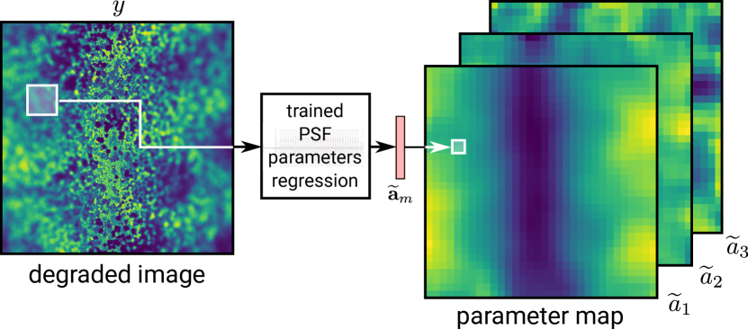
Figure 3: Spatially-variant PSF parameter mapping using a sliding window over the acquired image, as input of a convolutional neural network.

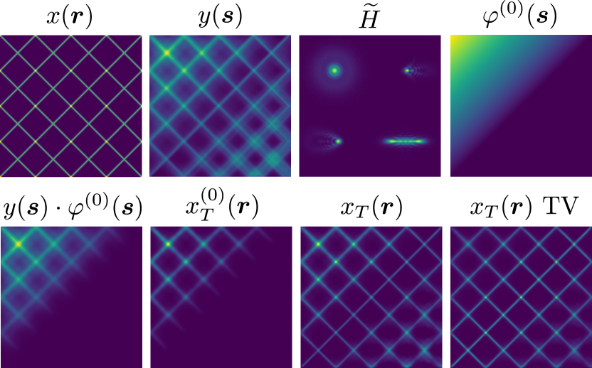
Figure 4: Synthetic experiment involving variables and results of Eq. (13). Starting from a ground truth image ($x(\bm{r})$), a local map of PSF (smooth interpolation between the 4 shown PSFs) and local weight combination $\bm{\varphi}(\bm{s})$, we generated a blurred image y. The deconvolution method (similar to [50] and [51]) starts from a map of locally estimated PSFs to deconvolve and recombine into a single image $x_{T}(\bm{r})$ and $x_{T}(\bm{r})$ TV.

II-G Application 1: spatially-variant blind deconvolution

We now turn to the problem of deconvolving the image. Existing deconvolution techniques can be categorized into three classes: (1) Non-blind methods, (2) entirely blind methods, and (3) parametric semi-blind algorithms. Non-blind methods require full knowledge of the PSF ([30], [52]), while the latter two classes aim at improving the image without prior knowledge of the PSF, the object, or other optical parameters. Entirely blind algorithms, such as [50] are based on optimization and estimation of the latent image or kernel [28]. Many blind deconvolution techniques are computationally expensive, especially for larger convolution kernels, and assume spatially invariant PSFs.

Parametric or semi-blind algorithms are blind methods that are constrained by knowledge about the transfer function distribution, such as a diffraction model or a prior on the shape of the PSF ([4], [53]). Parametric models allow reducing the complexity of the optimization problem, increasing the overall robustness, and avoiding issues such as over-fitting. However, it remains difficult to estimate the parameters from experimental data. We will focus on this third class of deconvolution methods, since our local PSF estimation method allows inferring their parameters without measuring any of them experimentally. Since we set a diffraction model defining the shape of the local PSF in a large image, we describe our deconvolution method as semi-blind.

Given the degraded image and a local map of PSF parameters, we restore the input using TV-RL deconvolution. Richardson-Lucy (RL) is an iterative maximum-likelihood approach and assumes that the noise follows a Poisson distribution [54], which is well adapted for microscopy. The method is subject to noise amplification, which can, however, be counterbalanced by a regularization term that penalizes the $l_{1}$ norm of the gradient of the signal ([55], [51]). Here, we assume that the PSF is spatially invariant in small parts of the image. Spatially-variant convolution techniques have been extensively reviewed by Denis et al. [56]. Hirsch et al. [50] have shown that the local invariance assumption can be improved by filtering the input with every local PSF and then reconstructing the image using interpolation. We extend this method by its inclusion in the TV-RL algorithm. Rather than interpolating deconvolved images, the overlap-add filtering method, as described in [50, 57], interpolates the PSF for each point in the image space. The idea for such method is: (i) to cover the image with overlapping patches using smooth interpolation, (ii) to deconvolve each patch with a different PSF, (iii) to add the patches to obtain a single large image. The equivalent for convolution can be written as:

$$x(\bm{r})=\sum_{m=0}^{M}(\widetilde{h}^{(m)}*(\varphi^{(m)}\odot y))(\bm{r}),$$ (12)

where $\varphi^{(m)}(\bm{s})$ is the masking operator of the $m$th patch. We illustrated the masking and deconvolution steps in Fig. 4. Since the RL algorithm tends to exacerbate edges and small variations such as noise, we use Total Variation (TV) regularization to obtain a smooth solution while preserving the borders [51]. The image at each RL iteration becomes:

$$x_{i+1}(\bm{r})=\sum_{m=0}^{M}\left[\frac{(\widetilde{h}^{(m)}*(\varphi^{(m)}\cdot y))(\mathord{\bm{r}})}{(\widetilde{h}^{(m)}*x^{(m)}_{i})(\mathord{\bm{r}})}*{\widetilde{h}^{(m)}}(\mathord{-\cdot})\right]\\ \cdot\frac{x^{(m)}_{i}(\bm{r})}{1-\lambda_{TV}\hskip 2.0pt\text{div}\left(\frac{\triangledown x^{(m)}_{i}(\bm{r})}{\lvert\triangledown x^{(m)}_{i}(\bm{r})\rvert}\right)},$$ (13)

with $y(\bm{s})$ the blurry image, $x_{i}(\bm{r})$ the deconvolved image at iteration $i=1,...,I$, $x^{(m)}_{i}(\bm{r})$ the $K_{y}\times L_{y}$ deconvolved patch at iteration $i$, $M$ the number of patches (and different PSFs) in one image $x$, $\widetilde{h}^{(m)}$ the $K_{h}\times L_{h}$ PSF for patch $m$ and $\lambda_{TV}$ the TV regularization factor. $\triangledown x_{i}^{j}(r)$ is the finite difference operator, which approximates the spatial gradient.

II-H Application 2: depth from focus using astigmatism

The spatially-variant PSF parameter mappings obtained in Section II-F yield local parameters, such as the blur, that are a function of the distance of the object to the focal plane. However, due to the symmetry of the PSF in depth, this function is ambiguous about the sign of the distance map $z(\bm{s})$ (above or below the focal plane). That is why we now aim at estimating the depth map $z(\bm{s})$ for every lateral pixel $\bm{s}$ of the 2D manifold in 3D space using our trained neural network and one single image as input. To achieve this, we use a local combination of Zernike polynomial coefficients $\bm{a}(\bm{s})$. The de-focus coefficient $a_{1}(\bm{s})$ is linked to the distance of the object to the focal plane, but there is no information about whether the object is in the front or behind the focal point. To address this limitation, we took inspiration from several methods to retrieve the relative position of a particle by encoding it in the shape of its PSF (either via use of astigmatic lenses ([38, 58]) or by use of a deformable mirror to generate more precise and complex PSF shapes [59]).

We used two cylindrical lenses of focal length $-400\text{\,}\mathrm{\SIUnitSymbolMicro m}$ and $400\text{\,}\mathrm{\SIUnitSymbolMicro m}$, separated by $3.4\text{\,}\mathrm{cm}$ thereby giving a combined focal length of $f=$6000\text{\,}\mathrm{mm}$$ and placed them in the infinity space of a microscope to generate an imaging system with an astigmatic PSF (Fig. 5). We used the networks trained in Section II-E1 using 2D-Zernike models to infer the depth map $z(\bm{s})$ from the 2D image $y(\bm{s}$) of the tridimensional surface $x_{\text{3D}}(\bm{r},z(\bm{r}))$. We defined a distance metric by multiplying the output focus parameter and the normalized and zero-centered astigmatism direction:

$$z(\bm{s})=a_{1}(\bm{s})\left(\frac{2a_{3}(\bm{s})}{\pi}-1\right),$$ (14)

with $a_{1}(\bm{s})$ the spatially local de-focus Zernike coefficient, and $a_{3}(\bm{s})\in(0,\pi)$ the spatially local Zernike coefficient encoding the direction of astigmatism.

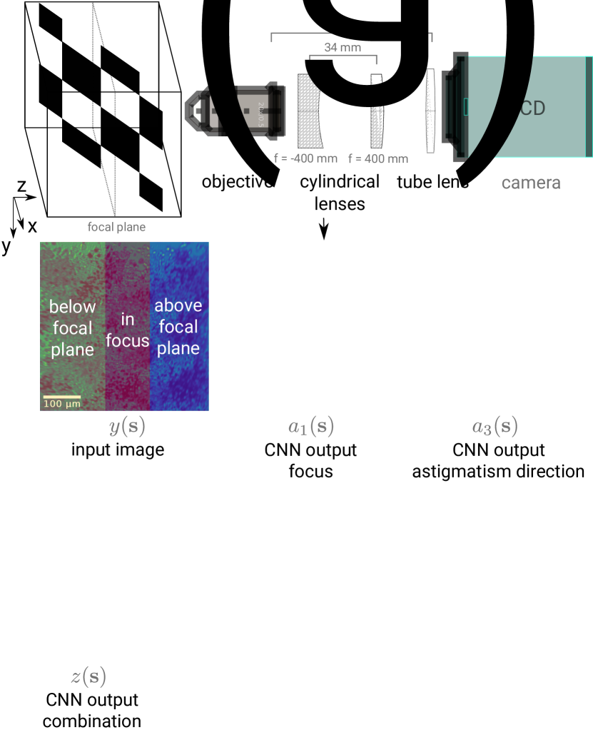
Figure 5: Depth estimation of a plane using controlled astigmatic aberrations by use of cylindrical lenses. (a) Optical system with using cylindrical lenses in the infinite tube space to induce astigmatism. (b) Image of a grid taken from the camera, with highlighted parts of the surface above and below the focal plane. (c),(d) Output of the CNN using (b) as input. The resolution of the map is $M=31\times 31$ different PSFs. (e) Weighted combination of (c) and (d) to form the depth map. (f) Projection of the depth of the surface over the $y$ axis and comparison to the ground truth data.

III Experiments

In this section we report our efforts to characterize the performance of our method as well as its dependency to several hyper-parameters, such as the choice of the PSF model, the neural network architecture, the training set size, or its content. We furthermore tested the regression performance of the PSF parameter regression and its robustness to Signal-to-Noise Ratio (SNR) degradation and the absence of texturing. Finally, we also assessed the quality of deconvolved images and the accuracy of the estimated depths.

III-A Infrastructure

Our PSF parameter estimation method depends on three main variables: the content and size of training data sets, the PSF parametric model and the neural network architecture. We briefly describe the different options below.

III-A1 Training, validation and test data sets for CNN regression performance

We gathered images from four different data sources:

1. [micr] microscopy images collected from [60], [61] and [62],

2. [nat] common images from the MIT Places365 data set [63] that gathers natural and man-made photographs,

3. [poi] synthetic images of points on a black background (Fig. 6),

4. [syn] synthetic images of cells (Fig. 6).

The rationale for using natural and synthetic images is that these data sources are much more abundant than microscopy images, often sharper and royalty free, making it possible to quickly assemble a large dataset. We combined these data to generate six different data sets (Table I) and prepared the library as described in Section II-E1. We randomly selected two times 10,000 images to form a validation set and an test dataset that the networks never use during the training process. The validation dataset is used for selecting the best learning rate and early stopping epoch for every training, while the testing set is used for performance assessment. We added synthetic black images to every data set to avoid misdetection of non-textured parts of the image and explicitly set ${a^{(k)}_{0}=1}$ for these samples.

TABLE I: Name and size of the different training, validation and test data sets as input of the CNN.

Data set	$K_{train}$	$K_{valid}$	$K_{test}$
syn	440,000	10,000	10,000
poi	330,000	10,000	10,000
micr	2,700,000	10,000	10,000
micrsm	270,000	10,000	10,000
nat	2,700,000	10,000	10,000
micr-syn-poi	3,470,000	10,000	10,000

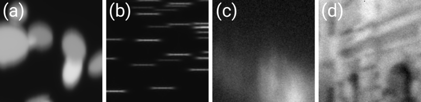
Figure 6: Examples of degraded input patches from different data sources: (a) synthetic cells [syn], (b) synthetic points [poi], (c) microscopy images [micr], (d) natural images [nat]. The images have been degraded by the Zernike-3 PSF model (see Table II) and noise as described in Section II-E1

.

III-A2 PSF models and parameters

We considered two different PSF model types: Zernike polynomials (Section II-B1) with $N=1,2,$ or $3$ parameters, and Gaussian (Section II-B2), with either $N=1$ or 2 parameters, as described in Table II.

TABLE II: PSF models selected for data set generation (Section II-E1), with the number and name of free parameters.

PSF model	$N$	Parameters
Zernike-1 (Z-1)	1	focus
Zernike-2 (Z-2)	2	cylinder, axis
Zernike-3 (Z-3)	3	focus, cylinder, axis
Gaussian-1 (G-1)	1	width
Gaussian-2 (G-2)	2	width x axis, width y axis

III-A3 CNN architectures and training modalities

We compared two residual neural networks architectures trained from scratch: 34-layer ResNet [46] and 50-layer ResNeXt [47]. They were adapted for accepting normalized gray-scale input image patches of size $W_{\psi}\times H_{\psi}=128\times 128$ pixels. Additionally, we fine-tuned, using our training dataset, the same network already trained on the ImageNet data set (available on the PyTorch website). For the latter model, we re-scaled the input images to the network input size using bilinear interpolation. We trained the models for 20 epochs with PyTorch 1.0 using the Adam optimizer [64] and a learning rate between $0.001$ and $0.01$ defined by the validation set performance.

III-B Characterization of the CNN regression performance

We analyzed the performance of our system for regressing the PSF parameters. The metrics we used to assess the performance of the network is the goodness-of-fit of the parameter estimation compared to the ground truth. We quantified it in terms of the squared Pearson correlation coefficient $R^{2}$ averaged over all PSF parameters:

$$R^{2}=\frac{1}{N}\sum_{n=0}^{N}{\left(1-\frac{\sum_{k=0}^{K_{\text{test}}-1}{(a^{(k)}_{n}-\widetilde{a}^{(k)}_{n})^{2}}}{\sum_{k=0}^{K_{\text{test}}-1}{(a^{(k)}_{n}-\bar{a}_{n})^{2}}}\right)},$$ (15)

with $K_{\text{test}}$ the number of samples in the test set. We calculated the correlation coefficient only for samples that contained texture in the ground-truth (i.e. when $a^{(k)}_{0}=0$) and discarded the others.

III-B1 Characterization of CNN regression performance when training and test data set types are the same

We started by assessing the performance of the CNNs when the test set is made of the same image type as the training set. Table III summarizes the performance of the regression of test data for every combination of training data sets (Table I), PSF models (Table II) and CNN architectures.

Variables: data set type, PSF model type, network architectures.

Fixed: the data set type is the same for training and testing.

Evaluation criterion: $R^{2}$ between the degradation parameters used to generate the test image and the parameters recovered by the CNN.

In most cases, the correlation coefficient is superior to 80%, which indicates a very good degree of overall correlation. The worst cases are with models trained for Zernike-3, that yield $0.61<R^{2}<0.96$. We notice a few differences in the regression performances between Gaussian and Zernike models. Indeed, images blurred with a Gaussian model tend to be better recognized by the neural network, with $R^{2}>0.90$, than images blurred with a Zernike model that fluctuates around $0.60<R^{2}<1.00$. When looking at the performance of a smaller [micr] training data set compared to the full [micr] data set, we notice that the performance of the smaller data set is always worse or equal, no matter which CNN model or PSF model used. Finally, we observe that the overall performance of ResNext-50 is lower than the performance of both ResNets.

TABLE III: Results of regression analyses (in terms of $R^{2}$) for $N=10,000$ test images in data sets shown in Table I using the same data type for training, validation (model selection) and test.

		ResNet-34
PSF models		[syn]	[poi]	[micr]	[micrsm]	[nat]	[micr-syn-poi]
	Z-1	0.99	0.99	0.98	0.73	0.98	0.68
	Z-2	0.67	0.99	0.81	0.80	0.80	0.79
	Z-3	0.95	0.98	0.78	0.58	0.84	0.88
	G-1	0.99	0.99	0.98	0.92	0.92	0.99
	G-2	0.99	0.99	0.99	0.97	0.91	0.99
		ResNet-34-pretrained
PSF models		[syn]	[poi]	[micr]	[micrsm]	[nat]	[micr-syn-poi]
	Z-1	0.99	0.99	0.99	0.89	0.99	0.81
	Z-2	0.93	0.97	0.92	0.81	0.94	0.90
	Z-3	0.97	0.89	0.95	0.77	0.80	0.89
	G-1	0.94	0.99	0.98	0.99	0.94	0.99
	G-2	0.99	0.99	0.99	0.98	0.95	0.99
		ResNext-50
PSF models		[syn]	[poi]	[micr]	[micrsm]	[nat]	[micr-syn-poi]
	Z-1	0.98	0.99	0.97	0.69	0.97	0.65
	Z-2	0.69	0.98	0.85	0.74	0.90	0.85
	Z-3	0.64	0.94	0.90	0.72	0.61	0.85
	G-1	0.99	0.99	0.97	0.80	0.91	0.98
	G-2	0.99	0.99	0.99	0.92	0.97	0.98

III-B2 Characterization of CNN regression performance when the type of training and test data set differ

We assessed the robustness of our regression method when the system is tested on image types other than those it has been trained for.

Variables: data set types for both training and test sets.

Fixed: the network architecture (ResNet-34), the PSF model (Gaussian-2). The model is already trained and selected using an independent validation dataset.

Evaluation criterion: $R^{2}$ between the degradation parameters used to generate the test input and the parameters recovered by the CNN.

Table IV gathers the regression performance obtained using a Gaussian-2 PSF model and the ResNet-34 network, with training and testing data sets of different types. The regression is robust to different train and test data set types ($R^{2}<0.90$) except when the CNN is trained with [poi] and, to a lesser extent, with [syn]. Surprisingly, networks trained on natural ([nat]) images perform as well as networks trained on microscopy images.

TABLE IV: Evaluation (in terms of $R^{2}$) for $N=10,000$ images input into a Resnet-34-pretrained network trained for regression of the Gaussian-2 PSF model parameters with different training set / test sets pairs. The learning rate and epoch were selected using results from a test set of $N=10,000$ separate images.

		Test data sets
Training data sets		[syn]	[poi]	[micr]	[micrsm]	[nat]	[micr-syn-poi]
	[syn]	1	0.93	0.76	0.83	0.81	0.85
	[poi]	0	1	0	0	0	0
	[micr]	0.97	0.97	0.99	0.99	0.99	0.99
	[micrsm]	0.97	0.95	0.95	0.98	0.89	0.97
	[nat]	0.99	0.80	0.96	0.93	0.96	0.96
	[micr-syn-poi]	1	0.99	0.99	0.99	0.94	0.99

III-C Robustness of PSF regression against input degradation

Degradations on the input images are unavoidable in biological environments. Indeed, microscopes are often used for a variety of sample types and preparations and are calibrated by different people. Settings such as illumination brightness, exposure time, and contrast frequently change or are operator-dependent. Furthermore, as described in Section II-E1, low light and electronics induce noise in the acquired image. Since we aim at training a regression network that is not specific to any defined acquisition condition, we characterized the robustness of the neural network to extrinsic modifications of the image quality.

The list of handled degradations is the following:

• global illumination level,

• non-uniform illumination (e.g. caused by poorly adjusted Köhler illumination),

• zero-mean Gaussian noise,

• signal-dependent Poisson noise,

• mixed Gaussian-Poisson noise.

Variables: degradation strength, degradation type, three different CNNs, two different PSF models (G-1, Z-1).

Fixed: the CNNs are already trained with [micr-syn-poi] and selected using an independent test dataset. The test data set is common to all modalities.

Evaluation criterion: $R^{2}$ between the degradation parameters that were used to generate the test image and the parameters recovered by the CNN.

Fig. 7 summarizes the performance of the CNN networks as a function of degradation strength. All networks are robust to partial or full brightness changes in the input image. The addition of Gaussian noise to the input results in a slow and linear decay in performance, whereas the application of Poisson noise to the data decrease the performance much faster as the noise strength increases. Using CNNs trained for regression of Zernike polynomial PSF model parameters, the regression performance is decaying linearly as a function of the amount of noise we apply in the input picture. For Gaussian models, the parameter estimation usually breaks with less noise than with the Zernike polynomial model. Without any degradation, networks regressing Zernike polynomials are less accurate than networks for Gaussian PSF models, but they appear to be more robust when the input is noisy. Indeed, with a very strong (strength of $0.5$ in Fig. 7) Gaussian and Poisson noise, Zernike-1 CNNs dropped from $R^{2}=0.95$ to $R^{2}=0.85$, as opposed to the Gaussian-1 CNNs, which dropped from $R^{2}=0.99$ to less than $R^{2}=0.60$. Surprisingly, contrary to the findings in a recent benchmark [45], we found that CNNs based on ResNeXt performed worse than their ResNet counterparts. Finally, we trained new models without adding synthetic noise to the training dataset (see Eq. (10)). Performance of these networks was the same as their counterparts for the illumination degradations, but dropped to $R^{2}=0$ when the test images contained even only moderate Poisson and Gaussian noise.

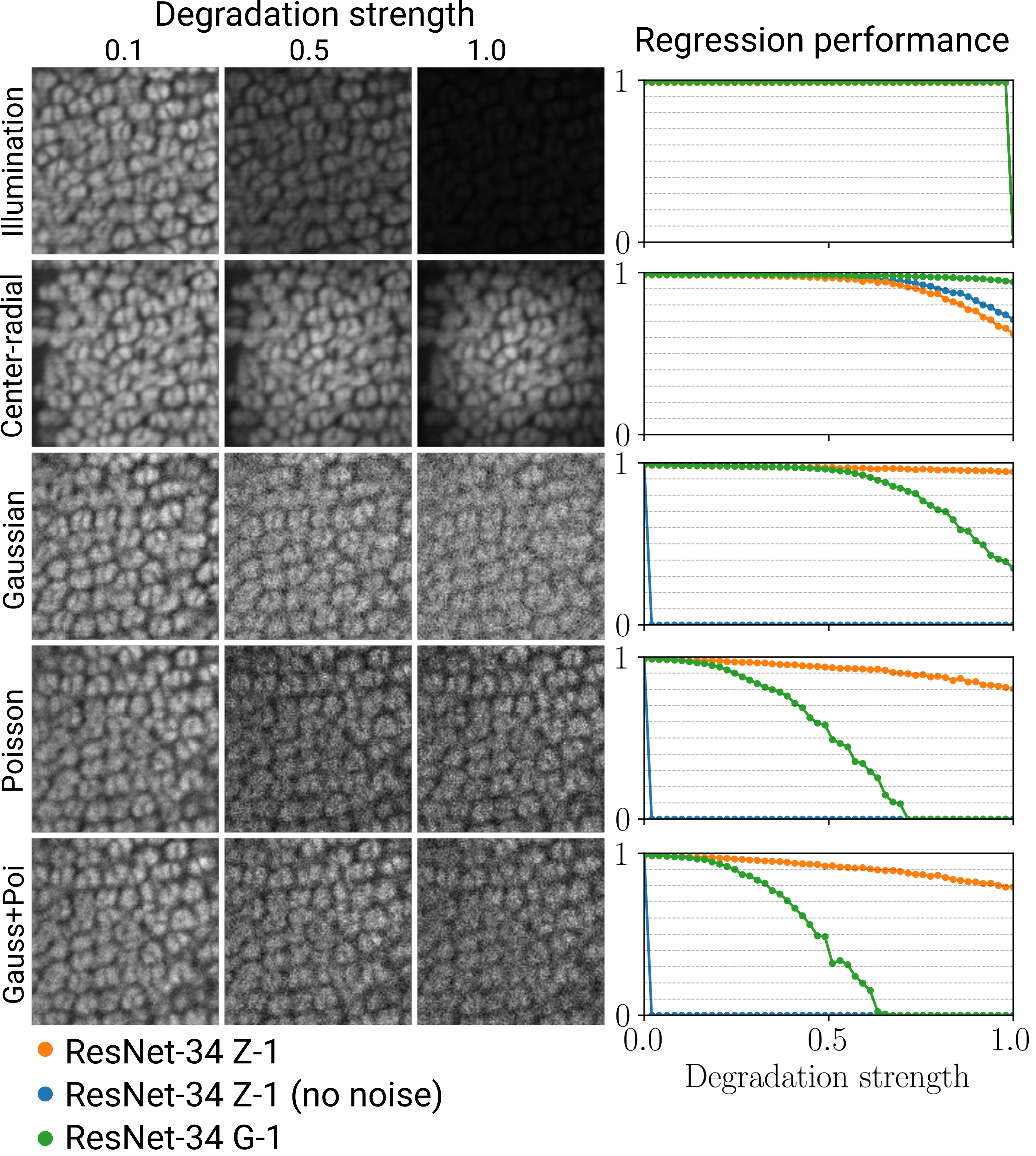
Figure 7: Regression performance of CNNs architectures trained on [micr] and evaluated on the [micr] test set with various types of degradation and variable strength. The regression performance is shown in terms of $R^{2}$ using $N=10,000$ images. We trained as well a CNN without adding noise in the training set (blue). All three networks exhibits the same performance for the illumination degradation (top right).

III-D Application 1: spatially-variant blind deconvolution

We next wanted to verify that the parameters recovered by the CNN were producing PSFs that are sufficiently accurate to be usable to enhance the details in the image, despite not being specifically measured. To this end, we devised a deconvolution experiment to compare images deconvolved by our method with those obtained by other blind deconvolution techniques. As test input, we used $256\times 256$ pixels image patches from the [micr] data set (see Section II-E1). Using Eq. (10), we degraded each quadrant of the input image with a specific, randomly-generated $127\times 127$ pixels PSFs using parameters $\bm{a}(\bm{s})$ drawn from a uniform random distribution allowing us to systematically explore the parameter space. We subsequently inferred a PSFs map via the CNN from the blurry image as described in Section II-F. Finally, we deconvolved the image by applying the method described in Section II-G. In the experiment, we set $\varphi^{(m)}$ as a bilinear interpolating function and, similarly to [51], $\lambda_{TV}=0.1$. Since using FFT-based calculations implies that the PSF is circulant, we took into account field extension to prevent spatial aliasing. We fixed the number $I$ of RL iterations to $20$.
We assessed the reconstruction quality by computing the SNR and Structural Similarity (SSIM) [65]. We compared the deconvolution results to spatially-invariant blind deconvolution techniques [66], [67] and [68], and the spatially-variant method from [69]. In the latter cases, we used the estimated PSF in the TV-RL algorithm with the same number of iterations and $\lambda_{TV}$. Since the estimation of a full PSF by these methods would take more than 20 minutes per sample, we constrained the support of the PSF to $31\times 31$ pixels. We computed the scores by taking the difference between the “ground truth” SNR and SSIM of images deconvolved using the PSFs actually used to degrade the images, and the deconvolution results using PSFs regressed with the CNN or other BD techniques. Theses values are therefore reported as $\Delta\text{SNR}$ and $\Delta\text{SSIM}$.
Finally, in order to recover details lost due to the aberrations of actual microscope objectives (such as out-of-focus blur and astigmatism), we acquired different fixed samples (HeLa cells actin (Alexa Fluor 635) and HeLa cells anti-$\alpha$-catenin (Alexa Fluor 488) with a 10$\times$/0.3 air objective, Convallaria majalis bulb autofluorescence with a 20$\times$/0.7 air objective) both in focus and slightly out of focus. Then, starting from a $256\times 256$ patch of the out-of-focus picture only, we sought to retrieve a sharper picture containing the details of the in-focus picture. We compared qualitatively the in-focus image, the out-of-focus image, our method with four PSFs detected with a $128\times 128$ stride, [66], [69], and the imaged obtained via a “sharpen” high-pass filter.

Variables: network architecture, two different PSF models (Z-1 and G-1) for the degradation and detection parts.

Fixed: CNNs are already trained, the test data set [micr] is fixed.

Evaluation criterion: difference of SNR and SSIM between the ground truth image and the deconvolved image.

Results in Table V indicate an average improvement of both SNR ($1.88$ dB) and SSIM ($0.09$) of our spatially variant BD. In comparison to spatially-invariant BD and other spatially-variant BD techniques improves the image by $1.55$ dB SNR and 0.08 SSIM. Deconvolution results are equivalent when the degradation and detection models are mismatched. The qualitative results shown in Fig. 8 highlight the stability of our method, which improves the degraded image to a detail level similar or better than the one of the in-focus image. Using the algorithm of Kotera et al. [66], the blurry features are well recovered, but the images have less detail. Furthermore, this algorithm converges to an aberrated image (Fig. 8 (b)) when the image contains long filaments. The method from Whyte et al. [69] enhances the contrast of the blurry image, however, it creates hallucinations near edges, which were not part of the original image. Finally, the high-pass filter, as expected, enhances both high-frequency features and noise.

TABLE V: Image deconvolution benchmark with 350 input images ($256\times 256$) from the test set [micr] for each experiment. We computed the difference in SNR and SSIM between the ground truth image and the deconvolved image. We compared the following methods: TV-RL with four known PSFs (gt), TV-RL with four PSFs estimated by the proposed CNN (CNN${}_{\text{blind}}$), Kotera et al., 2013 [66], Whyte et al., 2014 [69], Dong et al. [67] and Jin et al. [68]. The CNN is a ResNet-34 trained on data set [micr].

blurry		gt	CNN${}_{\text{blind}}$	Kotera [66]	Whyte [69]	Dong [67]	Jin [68]
Degradation	Detection	$\Delta\text{SNR}_{\text{gt}}$	$\Delta\text{SNR}_{\text{CNN-blind}}$	$\Delta\text{SNR}_{\text{\cite[cite]{[\@@bibref{}{kotera_blind_2013}{}{}]}}}$	$\Delta\text{SNR}_{\text{\cite[cite]{[\@@bibref{}{whyte_deblurring_2014}{}{}]}}}$	$\Delta\text{SNR}_{\text{\cite[cite]{[\@@bibref{}{dong_blind_2017}{}{}]}}}$	$\Delta\text{SNR}_{\text{\cite[cite]{[\@@bibref{}{jin_normalized_2018}{}{}]}}}$
Z-1	Z-1	$2.14\pm 0.71$	$\mathbf{1.65}\pm 0.62$	$-0.81\pm 0.71$	$0.12\pm 0.31$	$0.61\pm 0.58$	$1.34\pm 0.62$
Z-1	G-1	$2.14\pm 0.71$	$\mathbf{1.72}\pm 0.71$	$-0.61\pm 0.67$	$0.02\pm 0.31$	$0.83\pm 0.59$	$1.48\pm 0.67$
G-1	Z-1	$2.24\pm 0.73$	$\mathbf{2.02}\pm 1.04$	$-1.20\pm 0.97$	$-0.01\pm 0.55$	$0.89\pm 0.74$	$1.78\pm 0.76$
G-1	G-1	$2.24\pm 0.73$	$\mathbf{2.11}\pm 0.72$	$-1.25\pm 1.03$	$-0.31\pm 0.87$	$0.68\pm 0.9$	$1.58\pm 0.70$
		$\Delta\text{SSIM}_{\text{gt}}$	$\Delta\text{SSIM}_{\text{CNN-blind}}$	$\Delta\text{SSIM}_{\text{\cite[cite]{[\@@bibref{}{kotera_blind_2013}{}{}]}}}$	$\Delta\text{SSIM}_{\text{\cite[cite]{[\@@bibref{}{whyte_deblurring_2014}{}{}]}}}$	$\Delta\text{SSIM}_{\text{\cite[cite]{[\@@bibref{}{dong_blind_2017}{}{}]}}}$	$\Delta\text{SSIM}_{\text{\cite[cite]{[\@@bibref{}{jin_normalized_2018}{}{}]}}}$
Z-1	Z-1	$0.10\pm 0.03$	$\mathbf{0.10}\pm 0.04$	$0.05\pm 0.04$	$0.02\pm 0.02$	$0.09\pm 0.04$	$0.09\pm 0.04$
Z-1	G-1	$0.10\pm 0.03$	$\mathbf{0.09}\pm 0.03$	$0.03\pm 0.05$	$0.02\pm 0.01$	$0.08\pm 0.04$	$0.08\pm 0.03$
G-1	Z-1	$0.08\pm 0.03$	$0.08\pm 0.06$	$0.01\pm 0.05$	$0.01\pm 0.03$	$0.07\pm 0.04$	$\mathbf{0.08}\pm 0.03$
G-1	G-1	$0.08\pm 0.03$	$0.08\pm 0.04$	$0.01\pm 0.06$	$0.03\pm 0.03$	$0.07\pm 0.04$	$0.08\pm 0.04$

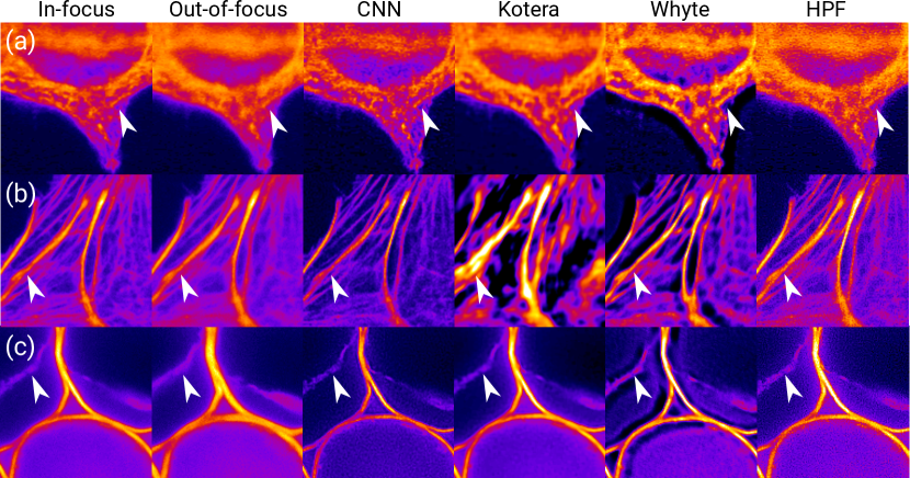
Figure 8: We acquired different fixed samples ((a) HeLa cells actin (Alexa Fluor 635) and (b) HeLa cells anti-$\alpha$-catenin (Alexa Fluor 488) with a 10$\times$/0.3 air objective, (c) Convallaria majalis bulb autofluorescence with a 20$\times$/0.7 air objective) both in-focus and slightly out-of-focus. Then, starting from a out-of-focus $256\times 256$ patch only, we seek to retrieve a sharper picture containing the details of the in-focus picture. We compared qualitative results of (from left to right), the in-focus image, the out-of-focus image, the proposed method (CNN) with four PSFs detected with a $128\times 128$ stride, [66], [69], and a ”sharpen” high-pass filter. Arrow edges indicate regions with features of particular interest.

III-E Application 2: depth from focus using astigmatism

The PSF parameter describing the local blur that we obtained from the image in Section II-F lacks information about the relative direction of the object from the focal plane. To infer the local axial distance map $z(\bm{s})$ in the sample, we applied the method described in Section II-H using the astigmatism created by a cylindrical lens. As an imaging sample, we used a grid of $$200\text{\,}\mathrm{\SIUnitSymbolMicro m}$\times$200\text{\,}\mathrm{\SIUnitSymbolMicro m}$$ squares which we laser-printed on a transparent plastic foil. We placed the grid towards the focal plane and tilted it by $3^{\circ}$, $6^{\circ}$, or $10^{\circ}$, so that the in-focus position was in the middle of the field of view (Fig. 5 (a)). With a field of view of $$655\text{\,}\mathrm{\SIUnitSymbolMicro m}$\times$655\text{\,}\mathrm{\SIUnitSymbolMicro m}$$, such a rotation yielded depth ranges of $48.2\text{\,}\mathrm{\SIUnitSymbolMicro m}$, $94.7\text{\,}\mathrm{\SIUnitSymbolMicro m}$, or $159.9\text{\,}\mathrm{\SIUnitSymbolMicro m}$, respectively.

We were able to retrieve the local Zernike coefficient parameters of focus ($a_{1}$), cylinder ($a_{2}$), and axis ($a_{3}$). We inferred the depth map $z(\bm{s})$ using Eq. (14) for $N=30$ acquired images in total (see Fig. 5 (e)).

Variables: input images of surfaces with a varying tilt angle from the focal plane.

Fixed: the network architecture (ResNet-34-pretrained for regression of Zernike parameters with astigmatism). CNNs are already trained, the test data set is fixed.

Evaluation criterion: $\ell_{1}$-error between the actual axial position of the surface and the position extracted from the image.

Using a CNN ResNet-34 trained with [micr], we obtained a correlation coefficient ($R^{2}$) between the average slope and a line fit of more than $0.96$. From this line fit we calibrated the system to spatial units so that we could build a depth map. The method was accurate with an absolute average $\ell_{1}$-error of $1.81\pm 1.39\text{\,}\mathrm{\SIUnitSymbolMicro m}$ in depth (corresponding to a $1.61\pm 1.23\%$ of the relative depth boundaries), obtained by comparing the error between the known position of the object in depth and the calibrated distance. Results in Table VI reveal that the relative error increases as the maximum depth of the object increases. Depth estimation is thus more precise around the focal plane.

TABLE VI: Analysis of the precision of the depth recovery of a plane using controlled astigmatic aberrations by use of cylindrical lenses. The test images are acquisitions of $N=30$ printed grids tilted 3^∘, 6^∘ and 10^∘. The network is a ResNet-34 trained on data set [micr].

Tilt angle	$R^{2}$	Absolute error	Relative error
10∘	0.967	$3.50\pm 2.62\text{\,}\mathrm{\SIUnitSymbolMicro m}$	$2.18\pm 1.64\%$
6∘	0.988	$1.31\pm 1.15\text{\,}\mathrm{\SIUnitSymbolMicro m}$	${1.38\pm 1.21}\%$
3∘	0.989	$0.61\pm 0.41\text{\,}\mathrm{\SIUnitSymbolMicro m}$	${1.26\pm 0.85}\%$

IV Discussion

Hereafter, we discuss the results of the experiments described in Section III.

IV-A Characterization of the CNN regression performance

Many regression accuracies are above $R^{2}=0.90$ in Table III, which shows that our neural networks can accurately regress PSF model parameters (in particular, when images are textured). The recovered parameters can be used to generate synthetic PSFs that are similar to the ones that degraded the image.
Our network is most accurate when applied to images of the same type as the ones used for training and the performance scales with the size of the training set. Therefore, the more data we gather, the more precise and robust the predictions are. However, adding synthetic training data to augment a natural images data set does not increase the efficacy of PSF estimations. The network fails to predict the PSF parameters if the network is trained with a very narrow type of data and more variety increases generalization potential. Nevertheless, when learning from a data set of images containing texture, even if different from the test set type, the model remains as accurate as when training the data set using microscopy images. This suggests that one could avoid the need to gather costly microscopy ground-truth data, or that it might be possible to learn from images of other microscope types (e.g. confocal microscopes) and use the trained models with wide field microscopy images. Furthermore, the high correlation score ($R^{2}>0.8$) obtained for [micr] test images using networks trained with [nat] suggests that the networks did not undergo overfitting and were able to generalize on other data types.
In comparison to ResNet-34, ResNeXt-50 requires a larger number of images to be accurate since the regression accuracy drops drastically (from $R^{2}=0.97$ to $R^{2}=0.79$) using a smaller data set. It is consistent with the general idea that the amount of training data must scale with the depth of the network to be able to generalize well.
Networks trained for Gaussian PSFs estimate parameters with a better accuracy than networks trained to find Zernike polynomials parameters. This could be explained by the fact that although the Zernike polynomial parameters are independent when describing the pupil function, they can compensate each other when forming the PSF (which is obtained by a non-linear operation on the pupil function, see Eq. (7)).
Using an NVIDIA GeForce GTX 1080 GPU, the estimation of the PSF parameters of a $1024\times 1024$ px image with 64 PSFs takes around $5.9\pm 0.1\text{\,}\mathrm{ms}$, which is in the same scale as the usual camera exposure time. This suggests that real-time applications in a microscope could be feasible.
While transfer learning (i.e. networks trained with ImageNet for image detection prior to training) does not help to improve the final accuracy of the regression task because the network was already able to learn from the original data set in a reasonable amount of time, training networks by starting from pre-trained models tends to speed up convergence during learning.

IV-B Robustness analysis against input degradation

We noticed that all our models are invariant to changes in illumination, certainly due to inherent normalization steps in the CNN architecture, and are overall robust to small to medium amounts of noise. However, when the signal-to-noise ratio strongly decreases, the correlation coefficient tends to decrease as well.

Additionally, we observed that, in comparison to ResNet, CNNs based on ResNeXt perform generally worse when noise is applied. This result contradicts observations reported in a recent benchmark [45], where ResNext is more robust than ResNet to Gaussian noise. However, this publication scores the network’s accuracy for a classification task into image type categories, which is a different application than our regression of aberrations and might explain the discrepancy.

We found the synthetic degradations we added in the training set (Eq. (10)) to be a necessary step to achieve robustness to noise. Indeed, the performance dropped when this step was omitted.

IV-C Application 1: spatially-variant blind deconvolution

Using the spatially-variant PSF map inferred from the PSF output, we have been able to reconstruct details in a degraded image without any prior information on the image content or the optical system. Given that our method does not require adjusting parameters or experimentally measuring a PSF (which is labor intensive), it leads to results faster than non-blind deconvolution methods.

We noticed that, because we use a constrained PSF model, our deconvolution method does not suffer from drawbacks sometimes associated to other deconvolution and super-resolution methods. For example, techniques based on MAP optimization sometimes converge to exotic forms of PSFs that are not consistent with the physics of optics, causing image deformation or loss of features [70]. We could illustrate this by the example in Fig.8 (b) for the method from Kotera et al. [66], which diverges when directed filaments are shown to the algorithm and creates artifacts.

Similarly, the use of denoising CNNs for image enhancement can lead to phantom details that could falsify underlying biological features, or discard high-frequency features that are mistaken for noise [71]. When using constrained PSF models such as the ones we use, deconvolution algorithms such as RL will still produce a reasonable image even if the predicted PSF is not exactly matching the PSF corresponding to the blur. This is likely due to the inherent constraint of a model with a small number of parameters that enforces the shape of the PSF. The outcome is a higher average SNR and SSIM of the reconstruction using our method compared to other BD algorithms. Another advantage of using constrained PSF models is that they can model PSFs with very large supports (sizes). Classical BD only allows for a smaller support, as using more pixels creates higher complexity. Nevertheless, our models are currently unlikely suitable for some types of degradation, where BD methods were successfully applied, such as for compensating for motion blur with rotation [72].

Deconvolution results are equivalently efficient both in terms of SNR and SSIM when the degradation and detection models are not similar (e.g. degradation using a Gaussian PSF and estimation of the PSF using a Zernike model). This particular point is relevant since it confirms the robustness of the image enhancement process when there is a mismatch between the degradation PSF that we want to model (i.e. the optical system PSF) and the model itself.

Finally, we observed that methods [69], [67] and [68], due to their multiscale optimization approach, were considerably slower than the one we propose, taking up to 4 minutes to deblur a $256\times 256$ image, whereas our method takes less than 3 seconds using the same machine to both estimate the PSF and perform TV-RL. The difference in run times can be explained by our GPU implementation, but as well because of the inherent nature of traditional optimization algorithms that alternate kernel and image estimation, which limits the parallelizability of the calculations.

IV-D Application 2: depth from focus using astigmatism

We showed that the focus parameter of the PSF models is a function of the distance between the sample and the focal plane, and that the sign of the axial distance could be recovered from higher Zernike coefficients when using engineered PSFs. Furthermore, we found that the depth function at any point in the image could be obtained from an affine function that combines two Zernike coefficients.

We recovered the relative depth of both sides of the printed grid in real microscopy acquisitions, which extends the idea of PSF engineering introduced in [58] for point-like structures, to work for fully textured images. Using a textured plane image, we have been able to recover the depth to up to $160\text{\,}\mathrm{\SIUnitSymbolMicro m}$. However, this accuracy decreases when the imaged objects lack texture. Using other shapes of engineered PSFs (e.g. quadripoles [59]) could potentially lead to improved depth accuracy.

Since use of an engineered PSF degrades the image, simultaneous depth retrieval and high-resolution might best be carried out by splitting the acquisition line (e.g. with a beam splitter) to record the image on one side and a PSF engineered image on the other.

Depth retrieval is also possible using the parameters of a Gaussian-2 PSF model, but the precision is improved using the PSF model based on Zernike polynomials.

V Conclusion

In this work, we have shown that CNNs, in particular residual networks, can be used to extract local blur characteristics from microscopy images in the form of parameters of a PSF model with only minimal knowledge about the optical setup. Our system is robust to signal perturbations and does not need to be trained specifically on images of the target imaging system. This flexibility allows the user to perform, without taking measurements beyond the images of interest, a wide range of tasks in microscopy image processing, including deblurring or obtaining a depth map.

Our method opens up the possibility to improve the resolution of non-flat objects with minimal a priori knowledge of the optical setup and obtain its tridimensional shape in a single shot.

Software sources, documentation, trained models, and the acquired test dataset (Fig. 8) will be made available upon publication. We thank Arne Seitz and José Artacho from EPFL BIOP for providing the fixed sample slides, reused from experiments that were approved by the EPFL Ethics Committee.

Appendix A References

References

- [1] Sarah Frisken Gibson and Frederick Lanni “Diffraction by a Circular Aperture as a Model for Three-Dimensional Optical Microscopy”, 1989, pp. 1357–1367 DOI: 10.1364/JOSAA.6.001357
- [2] Daniel Sage et al. “DeconvolutionLab2: An Open-Source Software for Deconvolution Microscopy” In Methods 115, 2017, pp. 28–41 DOI: 10.1016/j.ymeth.2016.12.015
- [3] P. Grossmann “Depth from Focus” In Pattern Recognit. Lett 5.1, 1987, pp. 63–69 DOI: 10.1016/0167-8655(87)90026-2
- [4] F. Aguet, D. Van De Ville and M. Unser “Model-Based 2.5-D Deconvolution for Extended Depth of Field in Brightfield Microscopy” In IEEE Trans Image Process 17.7, 2008, pp. 1144–1153 DOI: 10.1109/TIP.2008.924393
- [5] Asm Shihavuddin et al. “Smooth 2D Manifold Extraction from 3D Image Stack” In Nat Commun 8, 2017, pp. 15554 DOI: 10.1038/ncomms15554
- [6] Etienne Cuche, Pierre Marquet and Christian Depeursinge “Simultaneous Amplitude-Contrast and Quantitative Phase-Contrast Microscopy by Numerical Reconstruction of Fresnel off-Axis Holograms” In Appl. Opt. 38.34, 1999, pp. 6994 DOI: 10.1364/AO.38.006994
- [7] A. Griffa, N. Garin and D. Sage “Comparison of Deconvolution Software in 3D Microscopy: A User Point of View—Part 1” In G.I.T. Imaging & Microscopy 12.1, 2010, pp. 43–45 URL: http://infoscience.epfl.ch/record/163617
- [8] José-Angel Conchello and Jeff W Lichtman “Optical Sectioning Microscopy” In Nat Methods 2.12, 2005, pp. 920–931 DOI: 10.1038/nmeth815
- [9] Alex Krizhevsky, Ilya Sutskever and Geoffrey E Hinton “ImageNet Classification with Deep Convolutional Neural Networks” In NIPS Curran Associates, Inc., 2012, pp. 1097–1105 URL: http://papers.nips.cc/paper/4824-imagenet-classification-with-deep-convolutional-neural-networks.pdf
- [10] Shaoqing Ren, Kaiming He, Ross Girshick and Jian Sun “Faster R-CNN: Towards Real-Time Object Detection with Region Proposal Networks” In IEEE Trans. Pattern Anal. Mach. Intell 39.6, 2017, pp. 1137–1149 DOI: 10.1109/TPAMI.2016.2577031
- [11] Ross Girshick, Jeff Donahue, Trevor Darrell and Jitendra Malik “Rich Feature Hierarchies for Accurate Object Detection and Semantic Segmentation” In IEEE CVPR, 2014, pp. 580–587 arXiv: http://arxiv.org/abs/1311.2524
- [12] Samuel J. Yang et al. “Assessing Microscope Image Focus Quality with Deep Learning” In BMC Bioinformatics 19.1, 2018 DOI: 10.1186/s12859-018-2087-4
- [13] Xiang Zhu, Scott Cohen, Stephen Schiller and Peyman Milanfar “Estimating Spatially Varying Defocus Blur From A Single Image” In IEEE Trans. on Image Process. 22.12, 2013, pp. 4879–4891 DOI: 10.1109/TIP.2013.2279316
- [14] Jian Sun, Wenfei Cao, Zongben Xu and Jean Ponce “Learning a Convolutional Neural Network for Non-Uniform Motion Blur Removal” In IEEE CVPR 2015, 2015 arXiv: http://arxiv.org/abs/1503.00593
- [15] Dong Gong et al. “From Motion Blur to Motion Flow: A Deep Learning Solution for Removing Heterogeneous Motion Blur” In 2017 IEEE Conference on Computer Vision and Pattern Recognition (CVPR) Honolulu, HI: IEEE, 2017, pp. 3806–3815 DOI: 10.1109/CVPR.2017.405
- [16] Seungjun Nah, Tae Hyun Kim and Kyoung Mu Lee “Deep Multi-Scale Convolutional Neural Network for Dynamic Scene Deblurring” In IEEE CVPR, 2017
- [17] Adrian Shajkofci and Michael Liebling “Semi-Blind Spatially-Variant Deconvolution in Optical Microscopy with Local Point Spread Function Estimation by Use of Convolutional Neural Networks” In IEEE ICIP, 2018, pp. 3818–3822 arXiv: http://arxiv.org/abs/1803.07452
- [18] Da He, De Cai, Jiasheng Zhou, Jiajia Luo and Sung-Liang Chen “Restoration of Out-of-Focus Fluorescence Microscopy Images Using Learning-Based Depth-Variant Deconvolution” In IEEE Photonics Journal, 2020, pp. 1–1 DOI: 10.1109/JPHOT.2020.2974766
- [19] Martin Weigert et al. “Content-Aware Image Restoration: Pushing the Limits of Fluorescence Microscopy” In Nat Methods 15.12, 2018, pp. 1090–1097 DOI: 10.1038/s41592-018-0216-7
- [20] Yair Rivenson, Yibo Zhang, Harun Günaydın, Da Teng and Aydogan Ozcan “Phase Recovery and Holographic Image Reconstruction Using Deep Learning in Neural Networks” In Light Sci Appl 7.2, 2018, pp. 17141 DOI: 10.1038/lsa.2017.141
- [21] Yichen Wu et al. “Three-Dimensional Virtual Refocusing of Fluorescence Microscopy Images Using Deep Learning” In Nat Methods, 2019 DOI: 10.1038/s41592-019-0622-5
- [22] Hongda Wang et al. “Deep Learning Enables Cross-Modality Super-Resolution in Fluorescence Microscopy” In Nat Methods 16.1, 2019, pp. 103–110 DOI: 10.1038/s41592-018-0239-0
- [23] Joseph W. Goodman “Chapter 6-1” In Introduction To Fourier Optics Englewood, Colo: W.H.Freeman & Co Ltd, 2005, pp. 129
- [24] Bernard Chalmond “PSF Estimation for Image Deblurring” In CVGIP 53.4, 1991, pp. 364–372 DOI: 10.1016/1049-9652(91)90039-M
- [25] Neel Joshi, Richard Szeliski and David J. Kriegman “PSF Estimation Using Sharp Edge Prediction” In IEEE CVPR, 2008, pp. 1–8 DOI: 10.1109/CVPR.2008.4587834
- [26] Alexander Reuter, Hans-Peter Seidel and Ivo Ihrke “BlurTags: Spatially Varying PSF Estimation with out-of-Focus Patterns” In WSCG, 2012, pp. 9
- [27] Johannes Brauers, Claude Seiler and Til Aach “Direct PSF Estimation Using a Random Noise Target” In SPIE Electronic Imaging, 2010, pp. 75370B DOI: 10.1117/12.837591
- [28] A. Levin, Y. Weiss, F. Durand and W.. Freeman “Understanding Blind Deconvolution Algorithms” In IEEE Trans. Pattern Anal. Mach. Intell 33.12, 2011, pp. 2354–2367 DOI: 10.1109/TPAMI.2011.148
- [29] D.. Fish, A.. Brinicombe, E.. Pike and J.. Walker “Blind Deconvolution by Means of the Richardson–Lucy Algorithm” In J. Opt. Soc. Am. A 12.1, 1995, pp. 58–65 DOI: 10.1364/JOSAA.12.000058
- [30] F. Soulez “A “Learn 2D, Apply 3D” Method for 3D Deconvolution Microscopy” In IEEE ISBI, 2014, pp. 1075–1078 DOI: 10.1109/ISBI.2014.6868060
- [31] Jörg Herbel, Tomasz Kacprzak, Adam Amara, Alexandre Refregier and Aurelien Lucchi “Fast Point Spread Function Modeling with Deep Learning” In J. Cosmol. Astropart. Phys 2018.07, 2018, pp. 054–054 DOI: 10.1088/1475-7516/2018/07/054
- [32] Francois Aguet, Dimitri Van De Ville and Michael Unser “An Accurate PSF Model with Few Parameters for Axially Shift-Variant Deconvolution” In IEEE ISBI, 2008, pp. 157–160 DOI: 10.1109/ISBI.2008.4540956
- [33] G.. Airy “On the Diffraction of an Object-Glass with Circular Aperture” In Trans. Cambridge Philos. Soc. 5, 1835, pp. 283 URL: http://adsabs.harvard.edu/abs/1835TCaPS...5..283A
- [34] D.. Iskander, M.. Collins and B. Davis “Optimal Modeling of Corneal Surfaces with Zernike Polynomials” In IEEE Trans Biomed Eng 48.1, 2001, pp. 87–95 DOI: 10.1109/10.900255
- [35] F. Zernike “Beugungstheorie Des Schneidenver-Fahrens Und Seiner Verbesserten Form, Der Phasenkontrastmethode” In Physica 1.7, 1934, pp. 689–704 DOI: 10.1016/S0031-8914(34)80259-5
- [36] Joseph W. Goodman “Introduction to Fourier Optics” Roberts and Company Publishers, 2005 GOOGLEBOOKS: ow5xs˙Rtt9AC
- [37] Bo Zhang, Josiane Zerubia and Jean-Christophe Olivo-Marin “Gaussian Approximations of Fluorescence Microscope Point-Spread Function Models” In Appl. Opt. 46.10, 2007, pp. 1819–1829 DOI: 10.1364/AO.46.001819
- [38] H.. Kao and A.. Verkman “Tracking of Single Fluorescent Particles in Three Dimensions: Use of Cylindrical Optics to Encode Particle Position” In Biophys. J. 67.3, 1994, pp. 1291–1300 DOI: 10.1016/S0006-3495(94)80601-0
- [39] Yann A. LeCun, Léon Bottou, Genevieve B. Orr and Klaus-Robert Müller “Efficient Backprop” In Neural Networks: Tricks of the Trade Springer, 2012, pp. 9–48
- [40] F Luisier, Thierry Blu and M Unser “Image Denoising in Mixed Poisson–Gaussian Noise” In IEEE Trans. Image Process. 20.3, 2011, pp. 696–708 DOI: 10.1109/TIP.2010.2073477
- [41] E.. Gilbert and H.. Pollak “Amplitude Distribution of Shot Noise” In Bell System Technical Journal 39.2, 1960, pp. 333–350 DOI: 10.1002/j.1538-7305.1960.tb01603.x
- [42] Jia Deng, Wei Dong, Richard Socher, Li-Jia Li, Kai Li and Li Fei-Fei “ImageNet: A Large-Scale Hierarchical Image Database” In IEEE CVPR, 2009, pp. 8
- [43] Olga Russakovsky et al. “ImageNet Large Scale Visual Recognition Challenge” In Int J Comput Vis 115.3, 2015, pp. 211–252 DOI: 10.1007/s11263-015-0816-y
- [44] Jeff Donahue et al. “DeCAF: A Deep Convolutional Activation Feature for Generic Visual Recognition” In ICML, 2014, pp. 647–655 URL: http://proceedings.mlr.press/v32/donahue14.html
- [45] Dan Hendrycks and Thomas G. Dietterich “Benchmarking Neural Network Robustness to Common Corruptions and Surface Variations” In ICLR, 2019 arXiv: http://arxiv.org/abs/1807.01697
- [46] Kaiming He, Xiangyu Zhang, Shaoqing Ren and Jian Sun “Deep Residual Learning for Image Recognition” In IEEE CVPR, 2016, pp. 770–778 DOI: 10.1109/CVPR.2016.90
- [47] Saining Xie, Ross Girshick, Piotr Dollar, Zhuowen Tu and Kaiming He “Aggregated Residual Transformations for Deep Neural Networks” In IEEE CVPR, 2017, pp. 5987–5995 DOI: 10.1109/CVPR.2017.634
- [48] G. Huang, Z. Liu, L. Maaten and K.. Weinberger “Densely Connected Convolutional Networks” In IEEE CVPR, 2017, pp. 2261–2269 DOI: 10.1109/CVPR.2017.243
- [49] Klaus Hechenbichler and Klaus Schliep “Weighted K-Nearest-Neighbor Techniques and Ordinal Classification”, 2004 URL: https://www.econstor.eu/handle/10419/31150
- [50] Michael Hirsch, Suvrit Sra, Bernhard Scholkopf and Stefan Harmeling “Efficient Filter Flow for Space-Variant Multiframe Blind Deconvolution” In IEEE CVPR, 2010, pp. 607–614 DOI: 10.1109/CVPR.2010.5540158
- [51] Nicolas Dey et al. “Richardson–Lucy Algorithm with Total Variation Regularization for 3D Confocal Microscope Deconvolution” In Microsc. Res. Tech. 69.4, 2006, pp. 260–266 DOI: 10.1002/jemt.20294
- [52] Martin Weigert, Loic Royer, Florian Jug and Gene Myers “Isotropic Reconstruction of 3D Fluorescence Microscopy Images Using Convolutional Neural Networks” In MICCAI 10434, 2017, pp. 126–134 DOI: 10.1007/978-3-319-66185-8˙15
- [53] R. Morin, S. Bidon, A. Basarab and D. Kouamé “Semi-Blind Deconvolution for Resolution Enhancement in Ultrasound Imaging” In IEEE ICIP, 2013, pp. 1413–1417 DOI: 10.1109/ICIP.2013.6738290
- [54] William Hadley Richardson “Bayesian-Based Iterative Method of Image Restoration” In J. Opt. Soc. Am. 62.1, 1972, pp. 55–59 DOI: 10.1364/JOSA.62.000055
- [55] T.F. Chan and Chiu-Kwong Wong “Total Variation Blind Deconvolution” In IEEE Trans. on Image Process. 7.3, 1998, pp. 370–375 DOI: 10.1109/83.661187
- [56] Loïc Denis, Eric Thiébaut, Ferréol Soulez, Jean-Marie Becker and Rahul Mourya “Fast Approximations of Shift-Variant Blur” In Int. J. Comput. Vis 115.3, 2015, pp. 253–278 DOI: 10.1007/s11263-015-0817-x
- [57] M. Temerinac Ott, O. Ronneberger, R. Nitschke, W. Driever and H. Burkhardt “Spatially Variant Lucy-Richardson Deconvolution for Multiview Fusion of Microscopical 3D Images” In IEEE ISBI, 2011, pp. 899–904 DOI: 10.1109/ISBI.2011.5872549
- [58] Bo Huang, Wenqin Wang, Mark Bates and Xiaowei Zhuang “Three-Dimensional Super-Resolution Imaging by Stochastic Optical Reconstruction Microscopy” In Science 319.5864, 2008, pp. 810–813 DOI: 10.1126/science.1153529
- [59] Andrey Aristov, Benoit Lelandais, Elena Rensen and Christophe Zimmer “ZOLA-3D Allows Flexible 3D Localization Microscopy over an Adjustable Axial Range” In Nat Commun 9.1, 2018, pp. 2409 DOI: 10.1038/s41467-018-04709-4
- [60] Mark-Anthony Bray, Adam N. Fraser, Thomas P. Hasaka and Anne E. Carpenter “Workflow and Metrics for Image Quality Control in Large-Scale High-Content Screens” In J Biomol Screen 17.2, 2012, pp. 266–274 DOI: 10.1177/1087057111420292
- [61] Vebjorn Ljosa, Katherine L. Sokolnicki and Anne E. Carpenter “Annotated High-Throughput Microscopy Image Sets for Validation” In Nature Methods 9.7, 2012, pp. 637 DOI: 10.1038/nmeth.2083
- [62] Eleanor Williams et al. “The Image Data Resource: A Bioimage Data Integration and Publication Platform” In Nat Methods 14.8, 2017, pp. 775–781 DOI: 10.1038/nmeth.4326
- [63] B. Zhou, A. Lapedriza, A. Khosla, A. Oliva and A. Torralba “Places: A 10 Million Image Database for Scene Recognition” In IEEE Trans. Pattern Anal. Mach. Intell 40.6, 2018, pp. 1452–1464 DOI: 10.1109/TPAMI.2017.2723009
- [64] Diederik P. Kingma and Jimmy Ba “Adam: A Method for Stochastic Optimization” In ICLR, 2015 URL: http://arxiv.org/abs/1412.6980
- [65] Zhou Wang, Eero P. Simoncelli and Alan C. Bovik “Multiscale Structural Similarity for Image Quality Assessment” In IEEE ACSSC 2, 2004, pp. 1398–1402 URL: http://ieeexplore.ieee.org/abstract/document/1292216/
- [66] Jan Kotera, Filip Šroubek and Peyman Milanfar “Blind Deconvolution Using Alternating Maximum a Posteriori Estimation with Heavy-Tailed Priors” In CAIP Springer, 2013, pp. 59–66
- [67] Jiangxin Dong, Jinshan Pan, Zhixun Su and Ming-Hsuan Yang “Blind Image Deblurring with Outlier Handling” In 2017 IEEE International Conference on Computer Vision (ICCV), 2017, pp. 2497–2505 DOI: 10.1109/ICCV.2017.271
- [68] Meiguang Jin, Stefan Roth and Paolo Favaro “Normalized Blind Deconvolution” Cham: Springer International Publishing, 2018, pp. 694–711 DOI: 10.1007/978-3-030-01234-2˙41
- [69] Oliver Whyte, Josef Sivic and Andrew Zisserman “Deblurring Shaken and Partially Saturated Images” In Int. J. Comput. Vis 110.2, 2014, pp. 185–201 DOI: 10.1007/s11263-014-0727-3
- [70] Daniele Perrone and Paolo Favaro “Total Variation Blind Deconvolution: The Devil Is in the Details” In IEEE CVPR, 2014, pp. 2909–2916 DOI: 10.1109/CVPR.2014.372
- [71] Ding Liu, Bihan Wen, Xianming Liu, Zhangyang Wang and Thomas Huang “When Image Denoising Meets High-Level Vision Tasks: A Deep Learning Approach” In IJCAI, 2018, pp. 842–848 DOI: 10.24963/ijcai.2018/117
- [72] Qi Shan, Jiaya Jia and Aseem Agarwala “High-Quality Motion Deblurring from a Single Image” In ACM Trans. Graph. 27.3, 2008, pp. 1 DOI: 10.1145/1360612.1360672