Abstract

Continual learning (CL) is a setting in which an agent has to learn from an incoming stream of data during its entire lifetime. Although major advances have been made in the field, one recurring problem which remains unsolved is that of Catastrophic Forgetting (CF). While the issue has been extensively studied empirically, little attention has been paid from a theoretical angle. In this paper, we show that the impact of CF increases as two tasks increasingly align. We introduce a measure of task similarity called the NTK overlap matrix which is at the core of CF. We analyze common projected gradient algorithms and demonstrate how they mitigate forgetting. Then, we propose a variant of Orthogonal Gradient Descent (OGD) which leverages structure of the data through Principal Component Analysis (PCA). Experiments support our theoretical findings and show how our method can help reduce CF on classical CL datasets.

1 Introduction

Continual learning (CL) or lifelong learning [Thrun, 1995, Chen and Liu, 2018] has been one of the most important milestone on the path to building artificial general intelligence [Silver, 2011]. This setting refers to learning from an incoming stream of data, as well as leveraging previous knowledge for future tasks (through forward-backward transfer [Lopez-Paz and Ranzato, 2017]). While the topic has seen increasing interest in the past years [De Lange et al., 2019, Parisi et al., 2019] and a number of sohpisticated methods have been developed [Kirkpatrick et al., 2017, Lopez-Paz and Ranzato, 2017, Chaudhry et al., 2018, Aljundi et al., 2019b], a yet unsolved central challenge remains: Catastrophic Forgetting (CF) [Goodfellow et al., 2013, McCloskey and Cohen, 1989].

CF occurs when past solutions degrade while learning from new incoming tasks according to non-stationary distributions. Previous work either investigated this phenomenon empirically at different granularity levels (task level [Nguyen et al., 2019], neural network representations level [Ramasesh et al., 2020] ), or proposed a quantitative metric [Farquhar and Gal, 2018, Kemker et al., 2017, Nguyen et al., 2020].

Despite the vast set of existing works on CF, there is still few theoretical works studying this major topic. Recently, Bennani et al. [2020] propose a framework to study Continual Learning in the NTK regime then derive generalization guarantees of CL under the Neural Tangent Kernel [Jacot et al., 2018, NTK] for Orthogonal Gradient Descent [Farajtabar et al., 2020, OGD]. Following on this work, we propose a theoretical analysis of Catastrophic Forgetting for a family of projection algorithms including OGD, GEM [Lopez-Paz and Ranzato, 2017]. Our contributions can be summarized as follows:

• We provide a general definition of Catastrophic Forgetting, and examine the special case of CF under the Neural Tangent Kernel (NTK) regime. Our definition leverages the similarity between the source and target task.

• We derive the expression of the forgetting error for a family of orthogonal projection methods based on the NTK overlap matrix. This matrix reduces to the angle between the source and target tasks and is a critical component responsible for the Catastrophic Forgetting.

• For these projection methods, we analyze their mechanisms to reduce Catastrophic Forgetting and how they differ from each other.

• We propose PCA-OGD, an extension of OGD which mitigates the CF issue by compressing the relevant information into a reduced number of principal components. We show that our method is advantageous whenever the dataset has a dependence pattern between tasks.

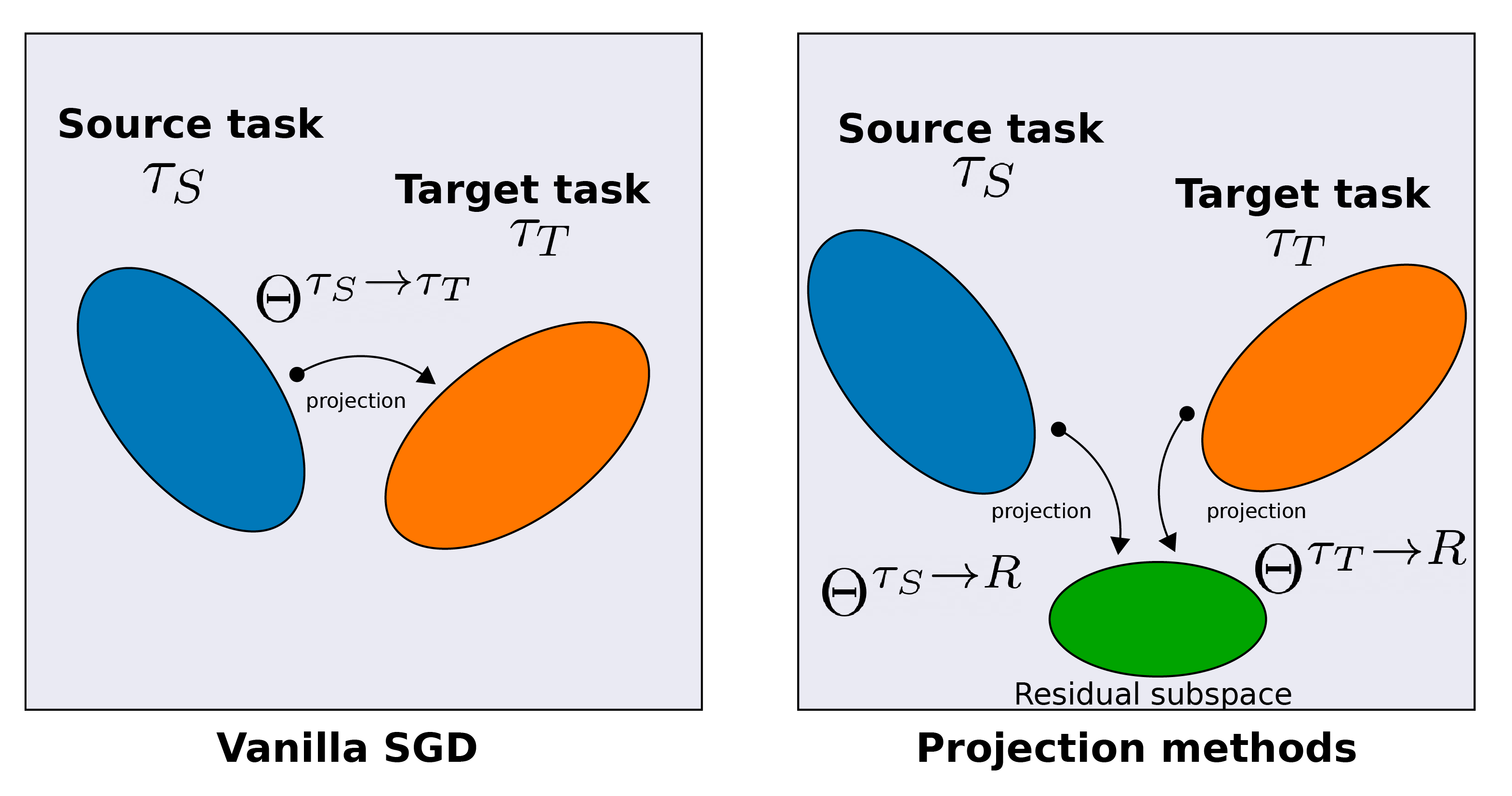
Figure 1: Unlike SGD, the projection methods reduce the forgetting by projecting the source and target tasks on a residual subspace.

2 Related Works

Defying Catastrophic Forgetting [McCloskey and Cohen, 1989] has always been an important challenge for the Continual Learning community. Among different families of methods, we can cite the following: regularization-based methods [Kirkpatrick et al., 2017, Zenke et al., 2017], memory-based and projection methods [Chaudhry et al., 2018, Lopez-Paz and Ranzato, 2017, Farajtabar et al., 2020] or parameters isolations [Mallya and Lazebnik, 2018, Rosenfeld and Tsotsos, 2018]. In [Pan et al., 2020], the authors propose a method to identify memorable example from the past that must be stored. An exhaustive list can be found in [De Lange et al., 2019]. Although theses methods achieve more or less success in combating Catastrophic Forgetting, its underlying theory remains unclear.

Recently, a lot of efforts has been put toward dissecting CF [Toneva et al., 2018]. While Nguyen et al. [2019] empirically studied the impact of tasks similarity on the forgetting, [Ramasesh et al., 2020] analyzed this phenomenon at the neural network layers level. [Xie et al., 2020] studied the designed artificial neural variability and studied its impact on the forgetting. Mirzadeh et al. [2020] investigated how different training regimes affected the forgetting. Other streams of works investigated different evaluation protocol and measure of CF [Farquhar and Gal, 2018, Kemker et al., 2017]. That being said, there is still few theoretical work confirming empirical evidences of CF.

Yin et al. [2020] provide an analysis of CL from a loss landscape perspective through a second-order Taylor approximation. Recent advances towards understanding neural networks behavior [Jacot et al., 2018] has enabled a better understanding through Neural Tangent Kernel (NTK) [Du et al., 2018, Arora et al., 2019]. Latest work and important milestone towards better theoretical understand of CL is from Bennani et al. [2020]. The authors provide a theoretical framework for CL under the NTK regime for the infinite memory case. Our work relaxes this constraint to the finite memory case, which is more applicable in the empirical setting.

3 Preliminaries

3.1 Notations

We use $\left\lVert\cdot\right\rVert_{2}$ to denote the Euclidian norm of a vector or the spectral norm of a matrix. We use $\langle\cdot,\cdot\rangle$ for the Euclidean dot product, and $\langle\cdot,\cdot\rangle_{\mathcal{H}}$ the dot product in the Hilbert space $\mathcal{H}$. We index the task ID by $\tau$. Learnable parameter are denoted $\omega$ and when indexing as $\omega_{\tau}$ correspond to the training during task $\tau$. Moreover $\star$ represents the variable at the end of a given task, i.e $w_{\tau}^{*}$ represents the learned parameters at the end of task $\tau$.

We denote $\mathbb{N}$ the set of natural numbers, $\mathbb{R}$ the space of real numbers and $\mbox{$\mathbb{N}$}^{\star}$ for the set $\mbox{$\mathbb{N}$}\smallsetminus\{0\}$.

3.2 Continual Learning

Let $\mathcal{X}$ be some feature space of interest (we take $\mathcal{X}=\mathbb{R}^{p}$), and let $\mathcal{Y}$ be the space of labels (we let $\mathcal{Y}=\mathbb{R}$, but $\mathcal{Y}=\Delta^{K}$ can be used for classification). In CL, we receive a stream of supervised learning tasks $\mbox{$\mathcal{T}$}_{\tau},\tau\in[T]$ where $\mbox{$\mathcal{T}$}_{\tau}=\{x^{\tau}_{j},y^{\tau}_{j}\}_{j=1}^{n_{\tau}}$, with $T\in\mathbb{N}^{*}$. While $X^{\tau}\in\mathbb{R}^{n_{\tau}\times p}$ ($p$ being the number of features) represents the dataset of task $\mbox{$\mathcal{T}$}_{\tau}$ and $x^{\tau}_{j}$, $j=1,...,n_{\tau}\in\mathcal{X}$ is a sample with its corresponding label $y^{\tau}_{j}\in\mathcal{Y}$. The goal is to learn a predictor $f_{\omega}:\mathcal{X}\times\mbox{$\mathcal{T}$}\rightarrow\mathcal{Y}$ with $\omega\in\mathbb{R}^{p}$ the parameters that will perform a prediction as accurate as possible. In the framework of CL, one cannot recover samples from previous tasks unless storing them in a memory buffer [Lopez-Paz and Ranzato, 2017, Parisi et al., 2019].

3.3 NTK framework for Continual Learning

Lee et al. [2019] recently proved that under the NTK regime neural networks evolve as a linear model:

$$f_{\tau}^{*}(x)=f_{\tau-1}^{*}(x)+\langle\nabla_{\omega}f_{0}(x),\omega_{\tau}^{*}-\omega_{\tau-1}^{*}\rangle$$

with $\omega_{\tau}^{\star}$ being the final weight after training on task $\tau$. The latter formulation implies the feature maps $\phi(x)=\nabla_{\omega}f_{0}(x)\in\mathbb{R}^{1\times p}$ is constant over time. Under that framework, [Bennani et al., 2020] show that CL models can be expressed as a recursive kernel regression and prove generalization and performance guarantee of OGD under infinite memory setting. We build up on this theoretical framework to study CF and quantify how the tasks similarity imply forgetting through the lens of eigenvalues and singular values decomposition (PCA and SVD).

4 Analysis of Catastrophic Forgetting in finite memory

In this section, we propose a general definition of Catastrophic Forgetting (CF). Casted in the NTK framework, this definition allows to understand what are the main sources of CF. Namely, CF is likely to occur when two tasks align significantly. Finally, we investigate CF properties for the vanilla case (SGD) and projection based methods such as OGD and a variant of GEM. We then introduce a new algorithm called PCA-OGD, an extension of OGD which reduces CF .

4.1 A definition of Catastrophic Forgetting under the NTK regime

A natural quantity to characterize CF is the change in predictions for the same input between a source task $\tau_{S}$ and target task $\tau_{T}$.

Definition 1 (Drift).

Let $\tau_{S}$ (respectively $\tau_{T}$) be the source task (respectively target task), $\mathcal{D}_{\tau_{S}}$ the source test set, the CF of task $\tau_{S}$ after training on all the subsequent tasks up to the target task $\tau_{T}$ is defined as:

$$\delta^{\tau_{S}\rightarrow\tau_{T}}(X^{\tau_{S}})=\Bigl{(}f^{\star}_{\tau_{T}}(x)-f^{\star}_{\tau_{S}}(x)\Bigr{)}_{(x,y)\in\mathcal{D}_{\tau_{S}}}$$ (1)

Note that $\delta^{\tau_{S}\rightarrow\tau_{T}}(X^{\tau_{S}})$ is a vector in $\mathbb{R}^{n_{\tau_{S}}}$ that contains the changes of predictions for any input $x$ in the task $\tau_{S}$. In the case of classification, we take the $k$-output of $f_{\tau}^{\star}$ such that $y_{k}=1$. In order to quantify the overall forgetting on this task, we use the squared norm of this vector.

Definition 2 (Catastrophic Forgetting).

Let $\tau_{S}$ (respectively $\tau_{T}$) be the source task (respectively target task), $\mathcal{D}_{\tau_{S}}$ the source test set, the CF of task $\tau_{S}$ after training on all subsequent tasks up to task $\tau_{T}$ is defined as:

$$\Delta^{\tau_{S}\rightarrow\tau_{T}}(X^{\tau_{S}}) =\|\delta^{\tau_{S}\rightarrow\tau_{T}}(X^{\tau_{S}})\|_{2}^{2}$$

$$=\sum_{(x,y)\in\mathcal{D}_{\tau_{S}}}(f^{\star}_{\tau_{T}}(x)-f^{\star}_{\tau_{S}}(x))^{2}$$ (2)

The above expression is very general but has an interesting linear form under the NTK regime and allows us to get insight on the behavior on the variation of the forgetting.

Lemma 1 (CF under NTK regime).

Let $\{\omega_{\tau}^{\star},\forall\tau\in[T]\}$ be the weight at the end of the training of task $\tau$, the Catastrophic Forgetting of a source task $\tau_{S}$ with respect to a target task $\tau_{T}$ is given by:

$$\Delta^{\tau_{S}\rightarrow\tau_{T}}(X^{\tau_{S}}) =\left\lVert\delta^{\tau_{S}\rightarrow\tau_{T}}(X^{\tau_{S}})\right\rVert_{2}^{2}$$ (3)

$$=\left\lVert\phi(X^{\tau_{S}})(\omega_{\tau_{T}}^{*}-\omega_{\tau_{S}}^{*})\right\rVert_{2}^{2}$$ (4)

Proof.

See Appendix Section 8.1. ∎

Lemma 1 expresses the forgetting as a linear relation between the kernel $\phi(X^{\tau_{S}})$ (which is assumed to be constant) and the variation of the weights from the source task $\tau_{S}$ until the target task $\tau_{T}$.

Remark 1.

Note that, from Equation 4, two cases are possible when $\Delta^{\tau_{S}\rightarrow\tau_{T}}(X^{\tau_{S}})=0$. The trivial case happens when $\forall\tau\in[T]$:

$$\Bigl{(}f^{\star}_{\tau+1}(x)-f^{\star}_{\tau}(x)\Bigr{)}_{(x,y)\in\mathcal{D}_{\tau_{S}}}=0$$

In this case, there is no drift at all. However, it is also possible that some tasks induce a drift on $X^{\tau_{S}}$ that is compensated by subsequent tasks. Indeed, for $\forall\tau\in[T]$:

$$0 =\delta^{\tau_{S}\rightarrow\tau_{T}}(X^{\tau_{S}})$$

$$=\Bigl{(}f^{\star}_{\tau_{T}}(x)-f^{\star}_{\tau_{S}}(x)\Bigr{)}_{(x,y)\in\mathcal{D}_{\tau_{S}}}$$

$$=\Bigl{(}f^{\star}_{\tau_{T}}(x)-f^{\star}_{\tau}(x)+f^{\star}_{\tau}(x)-f^{\star}_{\tau_{S}}(x)\Bigr{)}_{(x,y)\in\mathcal{D}_{\tau_{S}}}$$

simply implies, for any $(x,y)\in\mathcal{D}_{\tau_{S}}$,

$$f^{\star}_{\tau_{T}}(x)-f^{\star}_{\tau}(x)=-(f^{\star}_{\tau}(x)-f^{\star}_{\tau_{S}}(x)).$$

This would be an example of no forgetting due to a forward/backward transfer in the sense of Lopez-Paz and Ranzato [2017].

Now that we have defined the central quantity of this study, we will gain deeper insights by investigating SGD which is the vanilla algorithm.

4.2 High correlations across tasks induce forgetting for vanilla SGD

In this section, we derive the Catastrophic Forgetting expression for SGD. This will be the starting point to derive CF for the projection based methods (OGD, GEM and PCA-OGD).

Theorem 1.

(Catastrophic Forgetting for SGD)  Let $U_{\tau}\Sigma_{\tau}V_{\tau}^{T}$ be the SVD of $\phi(X^{\tau})$ for each $\tau\in[T]$, and let $\lambda>0$ the weight decay regularizer. The CF from task $\tau_{S}$ up until task $\tau_{T}$ is then given by:

$$\Delta^{\tau_{S}\rightarrow\tau_{T}}(X^{\tau_{S}})=\left\lVert\sum_{k=\tau_{S}+1}^{\tau_{T}}U_{\tau_{S}}\Sigma_{\tau_{S}}O^{\tau_{S}\rightarrow k}_{SGD}M_{k}\tilde{y}_{k}\right\rVert_{2}^{2}$$ (5)

where:

$$O^{\tau_{S}\rightarrow k}_{SGD} =V_{\tau_{S}}^{\top}V_{k}$$

$$M_{k} =\Sigma_{k}[\Sigma_{k}^{2}+\lambda I_{n_{k}}]^{-1}U_{k}^{\top}$$

$$\tilde{y}_{k} =y_{k}-f_{k-1}^{\star}(x^{k})$$

Proof.

See Appendix Section 8.2. ∎

Theorem 1 describes the Catastrophic Forgetting for SGD on the task $\mbox{$\mathcal{T}$}_{\tau_{S}}$ after training on the subsequent tasks up to the task $\mbox{$\mathcal{T}$}_{\tau_{T}}$. The CF is expressed as a function of the overlap between the subspaces of the subsequent tasks and the reference task, through what we call the NTK overlap matrices $\{O^{\tau_{S}\rightarrow k}_{SGD},k\in[\tau_{S}+1,\tau_{T}]\}$. High overlap between tasks increases the norm of the NTK overlap matrix which implies high forgetting.

More formally, the main elements of Catastrophic Forgetting are :

• $\Sigma_{\tau_{S}}$ encodes the importance of the principal components of the source task. Components with high magnitude contribute to forgetting since they imply high variation along thoses directions.

• $\{O^{\tau_{S}\rightarrow k}_{SGD},k\in[\tau_{S}+1,\tau_{T}]\}$ encodes the similarity of the principal components between the source task and a subsequent task $k$. High norm of this matrix means high overlap between tasks and leads to high risk of forgetting. This forgetting occurs because the previous knowledge along a given component may be erased by the new dataset.

• $\tilde{y}_{k}$ encodes the residual that remains to be learned by the current model. A null residual implies that the previous model predicts perfectly the new task, therefore there is no learning hence no forgetting.

• $M_{k}$ is a rotation of the residuals weighted by the principal components space. The rotated residuals $M_{k}\tilde{y}_{k}$ can be interpreted as the residuals along each principal component.

• $\left\lVert\sum_{k=\tau_{S}+1}^{\tau_{T}}\cdot\right\rVert$ encodes that the forgetting can be canceled by other tasks by learning again forgotten knowledge.

We will see in what follows that the matrix $O^{\tau_{S}\rightarrow\tau_{T}}_{SGD}$ captures the alignment between the source task $\tau_{S}$ and the target task $\tau_{T}$. More formally, the singular values of $O^{\tau_{S}\rightarrow\tau_{T}}_{SGD}$ are the cosines of the principal angles between the spaces spanned by the source data $\phi(X^{\tau_{S}})$ and the target data $\phi(X^{\tau_{T}})$ [Wedin, 1983].

Corollary 1 (Bounding CF with angle between source and target subspace).

Let $\Theta^{\tau_{S}\rightarrow\tau_{T}}$ be the diagonal matrix of singular values of $O^{\tau_{S}\rightarrow\tau_{T}}_{SGD}$ (each diagonal element $\cos(\theta_{\tau_{S},\tau_{T}})_{i}$ is the cosine of the $i$-th principal angle between $\phi(X^{\tau_{S}})$ and $\phi(X^{\tau_{T}})$). Let $\sigma_{\tau_{S},1}\geq\sigma_{\tau_{S},2}\geq...\geq\sigma_{\tau_{S},n_{\tau_{S}}}$ be the singular values of $\phi(X^{\tau_{S}})$ (i.e. the diagonal elements of $\Sigma_{\tau_{S}}$).

The bound of the forgetting from a source task $\tau_{S}$ up until a target task $\tau_{T}$ is given by:

$$\Delta^{\tau_{S}\rightarrow\tau_{T}}(X^{\tau_{S}})\leq\sigma_{\tau_{S},1}^{2}\sum_{k=\tau_{S}+1}^{\tau_{T}}\left\lVert\Theta^{\tau_{S}\rightarrow k}\right\rVert_{2}^{2}\left\lVert M_{k}\tilde{y}_{k}\right\rVert_{2}^{2}$$ (6)

Proof.

See Appendix Section 8.3. ∎

Corollary 1 bounds the CF by the sum of the cosines of the first principal angles between the source task $\tau_{S}$ and each subsequent task until the target task $\tau_{T}$ (represented by the diagonal matrix $\Theta^{\tau_{S}\rightarrow k}$) and a coefficient $\sigma_{\tau_{S},1}^{2}$ from the source task $\tau_{S}$.

• $\{\Theta^{\tau_{S}\rightarrow k},k\in[\tau_{S}+1,\tau_{T}]\}$ is the diagonal matrix where each element represents the cosine angle between subspaces $\tau_{S}$ and $k$: $\cos(\theta_{\tau_{S},k})_{i}$. If the principal angle between two tasks is small (i.e. the two tasks are aligned), the cosine will be large which implies a high risk of forgetting.

• $\sigma_{\tau_{S},1}$ is the variance of the data of task $\tau_{S}$ along its principal direction of variation. Intuitively, $\sigma_{\tau_{S},1}$ measures the spread of the data for task $\tau_{S}$.

In the end, a potential component responsible for CF in the Vanilla SGD case is the projection from the source task onto the target task. This phenomenon is best characterized by the eigenvalues of $O^{\tau_{S}\rightarrow\tau_{T}}_{SGD}$ which acts as a similarity measure between the tasks. One avenue to mitigate the CF can be to project orthogonally to the source task subspace which are the main insight from OGD [Farajtabar et al., 2020] and GEM [Lopez-Paz and Ranzato, 2017].

4.3 The effectiveness of the orthogonal projection against Catastrophic Forgetting

Now, we study the GEM and OGD algorithms, we identify these two algorithms as projection based algorithms. We extend the previous analysis to study the effectiveness of these algorithms against Catastrophic Forgetting.

Recap

OGD [Farajtabar et al., 2020] stores the feature maps of arbitrary samples from each task, then projects the update gradient orthogonally to these feature maps. The idea is to preserve the subspace spanned by the previous samples ([Yu et al., 2020] proposed a similar variant for multi-task learning ).

GEM [Lopez-Paz and Ranzato, 2017] computes the gradient of the train loss over each previous task, by storing samples from each task. While OGD performs an orthogonal projection to the gradients of the model, GEM projects orthogonally to the space spanned by the losses gradients. The idea is to update the model under the constraint that the train loss over the previous tasks does not increase.

GEM-NT : Decoupling Forward/Backward Transfer from Catastrophic Forgetting

OGD has been extensively studied by Bennani et al. [2020]), therefore we perform the analysis for the GEM algorithm, then highlight the similarities with OGD. Also, in order to decouple CF from Forward/Backward Transfer, we study a variant of GEM with no transfer at all, which we call GEM No Transfer (GEM-NT).

Similarly to GEM, GEM-NT maintains an episodic memory containing $d$ samples from each previous tasks seen so far. During each gradient step of task $\tau+1$, GEM samples from the memory $d$ elements from each previous task then compute the average loss function gradient:

$$g_{k}=\frac{1}{d}\displaystyle{\sum_{j=1}^{d}}\nabla_{\omega}\mathcal{L}^{k}_{\lambda}(x^{k}_{j}),\quad\forall k=1,..,\tau$$

If the proposed update during task $\tau+1$ can potentially degrades former solutions (i.e $\langle g_{\tau+1},g_{k}\rangle<0,\forall k\leq\tau$) then the proposed update is projected orthogonally to these gradients $g_{k}$, $\forall k\leq\tau$.

As opposed to GEM, which performs the orthogonal projection conditionally on the impact of the gradient update on the previous training losses, GEM-NT project orthogonally to $g_{k}$, $\forall k\leq\tau$ at each step irrespectively of the sign of the dot product. The algorithm pseudo-code can be found in Appendix Section 2.

The effectiveness of GEM-NT against CF

Denote $G_{\tau}\in\mathbb{R}^{p\times\tau}$ the matrix where each columns represents $g_{k},\forall k=1,..,\tau$, the orthogonal projection matrix is then defined as $T_{\tau}=I_{p}-G_{\tau}G_{\tau}^{\top}=\overline{G}_{\tau}\overline{G}_{\tau}^{\top}$. This represents an orthogonal projection whatever the sign of the dot product $\langle g_{\tau+1},g_{k}\rangle$ in order to decouple the forgetting from transfer.

We are now ready to provide the CF of GEM-NT.

Corollary 2 (CF for GEM-NT).

Using the previous notations. The CF from task $\tau_{S}$ up until task $\tau_{T}$ for GEM-NT given by:

$$\Delta^{\tau_{S}\rightarrow\tau_{T}}(X^{\tau_{S}})=\left\lVert\sum_{k=\tau_{S}+1}^{\tau_{T}}U_{\tau_{S}}\Sigma_{\tau_{S}}{\color[rgb]{0.17254901960784313,0.6274509803921569,0.17254901960784313}\mathbf{O^{\tau_{S}\rightarrow k}_{\text{GEM-NT}}}M_{k}}\tilde{y}_{k}\right\rVert_{2}^{2}$$ (7)

where:

$$O^{\tau_{S}\rightarrow k}_{\text{GEM-NT}} =V_{\tau_{S}}^{\top}{\color[rgb]{0.17254901960784313,0.6274509803921569,0.17254901960784313}\overline{G}_{k-1}\overline{G}_{k-1}^{\top}}V_{k}$$

$$M_{k} =\Sigma_{k}U_{k}^{\top}[{\color[rgb]{0.17254901960784313,0.6274509803921569,0.17254901960784313}\overline{\phi}(X^{k})\overline{\phi}(X^{k})^{\top}}+\lambda I_{n_{k}}]^{-1}$$

$$\overline{\phi}(X^{k}) =\phi(X^{k})T_{k-1}$$

(Differences with the vanilla case SGD are highlighted in color)

Proof.

See Appendix Section 8.4. ∎

The difference for GEM-NT lies in the double projection of the source and target task onto the subspace $\overline{G}_{\tau}$ which contain elements orthogonal to $g_{k},\forall k=1,..,\tau-1$.

Similarly to Corollary 1, we can bound each projection matrix ($V_{\tau_{S}}^{\top}\overline{G}_{k-1}$ and $\overline{G}_{k-1}^{\top}V_{k}$,$\forall k\in[\tau_{S}+1,\tau_{T}]$ ) by their respective matrices of singular values ($\Theta^{\tau_{S}\rightarrow G_{k-1}}$ and $\Theta^{k\rightarrow G_{k-1}}$, $\forall k\in[\tau_{S}+1,\tau_{T}]$). This leads us to the following upper-bound for the CF of GEM-NT:

$$\Delta^{\tau_{S}\rightarrow\tau_{T}}(X^{\tau_{S}})\leq$$ (8)

$$\sigma_{\tau_{S},1}^{2}\sum_{k=\tau_{S}+1}^{\tau_{T}}{\color[rgb]{0.17254901960784313,0.6274509803921569,0.17254901960784313}\left\lVert\Theta^{\tau_{S}\rightarrow\overline{G}_{k-1}}\right\rVert_{2}^{2}\left\lVert\Theta^{k\rightarrow\overline{G}_{k-1}}\right\rVert_{2}^{2}}\left\lVert M_{k}\tilde{y}_{k}\right\rVert_{2}^{2}$$

Connection of GEM-NT to OGD

For the analysis purpose, let’s suppose that the memory per task is $1$, $\lambda=0$, $\forall\tau\in[T]$ and assume a mean square loss error function. In that case:

$$g_{k}=\begin{cases}\nabla_{\omega}f_{k}(x)(f_{k}(x)-y_{k})\quad&(\text{GEM-NT})\\ \nabla_{\omega}f_{k}(x)\quad\quad&(\text{OGD})\end{cases}$$ (9)

• unlike OGD, GEM-NT weights the orthogonal projection with the residuals $(f_{\tau}(x^{k})-y_{k})=(\tilde{y}_{k}+\delta^{k\rightarrow\tau}(x^{k}))$ which represents the difference between the new prediction (due to the drift) for $x^{k}$ under model $\tau$ and the target $y_{k}$.

• Previous tasks that are well learned (small residuals) will contribute less to the orthogonal projection to the detriment of tasks with large residuals (badly learned then). This seems counter-intuitive because by doing so, the projection will not be orthogonal to well learned tasks (in the edge case of zero residuals) then unlearning can happen for those tasks.

While OGD and GEM-NT are more robust to CF than SGD through the orthogonal projection, they do not leverage explicitely the structure in the data [Farquhar and Gal, 2018]. We can then compress this information through dimension reduction algorithms such as SVD in order to both maximise the information contained in the memory as well as mitigating the CF.

4.4 PCA-OGD: leveraging structure by projecting orthogonally to the top d principal directions

Unlike OGD that stores randomly $d$ samples from each task $k=1,..,\tau$ of $\{\nabla_{\omega}f(x^{k}_{j})\}_{j=1}^{d}$, at the end of each task $\tau$, PCA-OGD samples randomly $s>d$ elements from $X^{\tau}$ then stores the top $d$ eigenvectors of $\{\nabla_{\omega}f(X^{\tau})\}$ denoted as $v_{\tau,i}$, $i=1,..,d$. These are the directions that capture the most variance of the data. If we denote by $P_{\tau,:d}$ the matrix where each columns represents $v_{k,i}$, $k=1,..,\tau$, $i=1,..,d$ then the orthogonal matrix projection can be written as:

$$T_{\tau,:d}=I_{p}-P_{\tau,:d}P_{\tau,:d}^{\top}=R_{\tau,d:}R_{\tau,d:}^{\top}$$ (10)

where the columns of $R_{\tau,d:}$ form an orthonormal basis of the orthogonal complement of the span of $P_{\tau,:d}$. For the terminology, $P_{\tau,:d}\in\mathbb{R}^{p\times(\tau\cdot d)}$ (respectively $R_{\tau,d:}\in\mathbb{R}^{p\times p-(\tau\cdot d)}$) represents the top subspace (respectively the residuals subspace) of order $d$ for task $1$ until $\tau$. A pseudo-code of PCA-OGD is given in Alg. 1 (the computational overhead can be found in the Appendix). We are now ready to provide the CF of PCA-OGD.

Input : A task sequence $\mbox{$\mathcal{T}$}_{1},\mbox{$\mathcal{T}$}_{2},\ldots$, learning rate $\eta$, PCA samples $s$, components to keep $d$

1. Initialize $S_{J}\leftarrow\{\}$ ; $\omega\leftarrow\omega_{0}$

2. for Task ID $\tau=1,2,3,\ldots$ do

       repeat

             $\mbox{$\mbox{$\mathbf{g}$}$}\leftarrow$ Stochastic Batch Gradient for $\mbox{$\mathcal{T}$}_{\tau}$ at $\omega$;

             // Orthogonal updates $\tilde{\mbox{$\mbox{$\mathbf{g}$}$}}=\mbox{$\mbox{$\mathbf{g}$}$}-\sum_{\mbox{$\mbox{$\mathbf{v}$}$}\in\mbox{$\mathcal{S}$}_{J}}\mathrm{proj}_{\mbox{$\mbox{$\mathbf{v}$}$}}(\mbox{$\mbox{$\mathbf{g}$}$})$;

             $\omega\leftarrow\omega-\eta\tilde{\mbox{$\mbox{$\mathbf{g}$}$}}$

      until convergence;

      // Gram-Schmidt orthogonalization for $(\mbox{$\mbox{$\mathbf{x}$}$},y)\in\mathcal{D}_{\tau}$ and $k\in[1,c]$ s.t. $y_{k}=1$ do

             $\mbox{$\mbox{$\mathbf{u}$}$}\leftarrow\nabla f_{\tau}(\mbox{$\mbox{$\mathbf{x}$}$};\omega)-\sum_{\mbox{$\mbox{$\mathbf{v}$}$}\in\mbox{$\mathcal{S}$}_{J}}\mathrm{proj}_{\mbox{$\mbox{$\mathbf{v}$}$}}(\nabla_{\omega}f_{\tau}(\mbox{$\mbox{$\mathbf{x}$}$};\omega))$ $\mbox{$\mathcal{S}$}_{J}\leftarrow\mbox{$\mathcal{S}$}_{J}\bigcup\{\mbox{$\mbox{$\mathbf{u}$}$}\}$

       end for

      // PCA Sample $s$ elements from $\mbox{$\mathcal{T}$}_{\tau}$

       top $d$ eigenvectors $\leftarrow PCA(\{\nabla_{\omega}f_{\tau}(x^{\tau}_{j})\}_{j=1}^{s})$   $\mbox{$\mathcal{S}$}_{J}\leftarrow\mbox{$\mathcal{S}$}_{J}\bigcup\ \{$ top $d$ eigenvectors $\}$  

end for

Algorithm 1 PCA-OGD (Differences with OGD in red)

Corollary 3 (Forgetting for PCA-OGD).

For each $\tau\in[T]$, let $\tilde{\phi}(X^{\tau})=\phi(X^{\tau})T_{\tau-1,:d}$ and let $U_{\tau}\Sigma_{\tau}V_{\tau}^{T}$ be the SVD of $\phi(X^{\tau})$. The CF for PCA-OGD is given by:

$$\Delta^{\tau_{S}\rightarrow\tau_{T}}(X^{\tau_{S}})=\left\lVert\sum_{k=\tau_{S}+1}^{\tau_{T}}{\color[rgb]{0.12156862745098039,0.4666666666666667,0.7058823529411765}\mathbf{U_{\tau_{S}}\Sigma_{\tau_{S}}O^{\tau_{S}\rightarrow k}_{PCA}}M_{k}}\tilde{y}_{k}\right\rVert_{2}^{2}$$ (11)

where:

$$O^{\tau\rightarrow k}_{PCA} =V_{\tau_{S}}^{\top}{\color[rgb]{0.12156862745098039,0.4666666666666667,0.7058823529411765}R_{k-1,d:}R_{k-1,d:}^{\top}}V_{k}$$

$$M_{k} =\Sigma_{k}U_{k}^{\top}[{\color[rgb]{0.12156862745098039,0.4666666666666667,0.7058823529411765}\tilde{\phi}(X^{k})\tilde{\phi}(X^{k})^{\top}}+\lambda I_{n_{k}}]^{-1}$$

$$\tilde{\phi}(X^{k}) =\phi(X^{k})T_{k-1,:d}$$

Proof.

See Appendix Section 8.5. ∎

Corollary 3 underlines the difference with GEM-NT as this time the double projection are on the residuals subspace $R_{k-1,:d}$ containing the orthogoanl vector to the features map $\nabla_{\omega}f(x)$ instead of the loss function gradient.

Remark 2.

• PCA is helpful in datasets where the eigenvalues are decreasing exponentially since keeping a small number of components can leverage a large information and explain a great part of the variance. Projecting orthogonally to these main components will lead to small forgetting if $\sigma_{\tau,d+1}$ is small.

• On the other hand, unfavourable situations where data are spread uniformly along all directions (i.e, eigenvalues are uniformly equals ) will requires to keep all components and a larger memory. As an example, we build a worst-case scenario in Appendix Section 8.12 where OGD is performing better than PCA-OGD.

Similarly as the previous case, we can bound the double projection on $R_{k-1,:d}$ with the corresponding diagonal matrix $\Theta^{\tau_{S}\rightarrow R_{k,:d}}$. Additionally, the CF is bounded by $\sigma_{\tau_{S},d+1}$ which is due to the orthogonal projection to the first $d$ principal directions. The upper bound of the CF is given by:

$$\Delta^{\tau_{S}\rightarrow\tau_{T}}(X^{\tau})\leq$$ (12)

$${\color[rgb]{0.12156862745098039,0.4666666666666667,0.7058823529411765}\mathbf{\sigma_{\tau_{S},d+1}^{2}}}\sum_{k=\tau_{S}+1}^{\tau_{T}}{\color[rgb]{0.12156862745098039,0.4666666666666667,0.7058823529411765}\mathbf{\left\lVert\Theta^{\tau_{S}\rightarrow R_{k-1,:d}}\right\rVert_{2}^{2}\left\lVert\Theta^{k\rightarrow R_{k-1,:d}}\right\rVert_{2}^{2}}}\left\lVert M_{k}\tilde{y}^{k}\right\rVert_{2}^{2}$$

Note that in contrast with Eq. (8), the first term in the upper bound is the ($d+1$)-th singular value of $\phi(X^{\tau_{S}})$, which is due to the PCA step of PCA-OGD. A summary of the forgetting properties of the described methods can be found in Table 2 in Appendix.

5 Experiments

In this section, we study the impact of the NTK overlap matrix on the forgetting by validating Corollary 1. We then illustrates how PCA-OGD efficiently captures and compresses the information in datasets (Corollary 3. Finally, we benchmark PCA-OGD on standard CL baselines.

5.1 Low eigenvalue of the NTK overlap matrix induces smaller drop in performance

Objective :

As presented in Corollary 1, we want to assess the effect of the eigenvalues of the NTK overlap matrix on the forgetting.

Experiments :

We measure the drop in accuracy for task $1$ until task $15$ on Rotated MNIST with respect to the maximum eigenvalue of the NTK overlap matrix $O^{1\rightarrow 15}$.

Results :

Figure 2 shows the drop in accuracy between task $1$ and task $15$ for Rotated MNIST versus the largest eigenvalue of $O^{1\rightarrow 15}$. As expected low eigenvalues leads to a smaller drop in accuracy and thus less forgetting. PCA-OGD improves upon OGD, having from $7\%$ to $10\%$ less drop in performance.

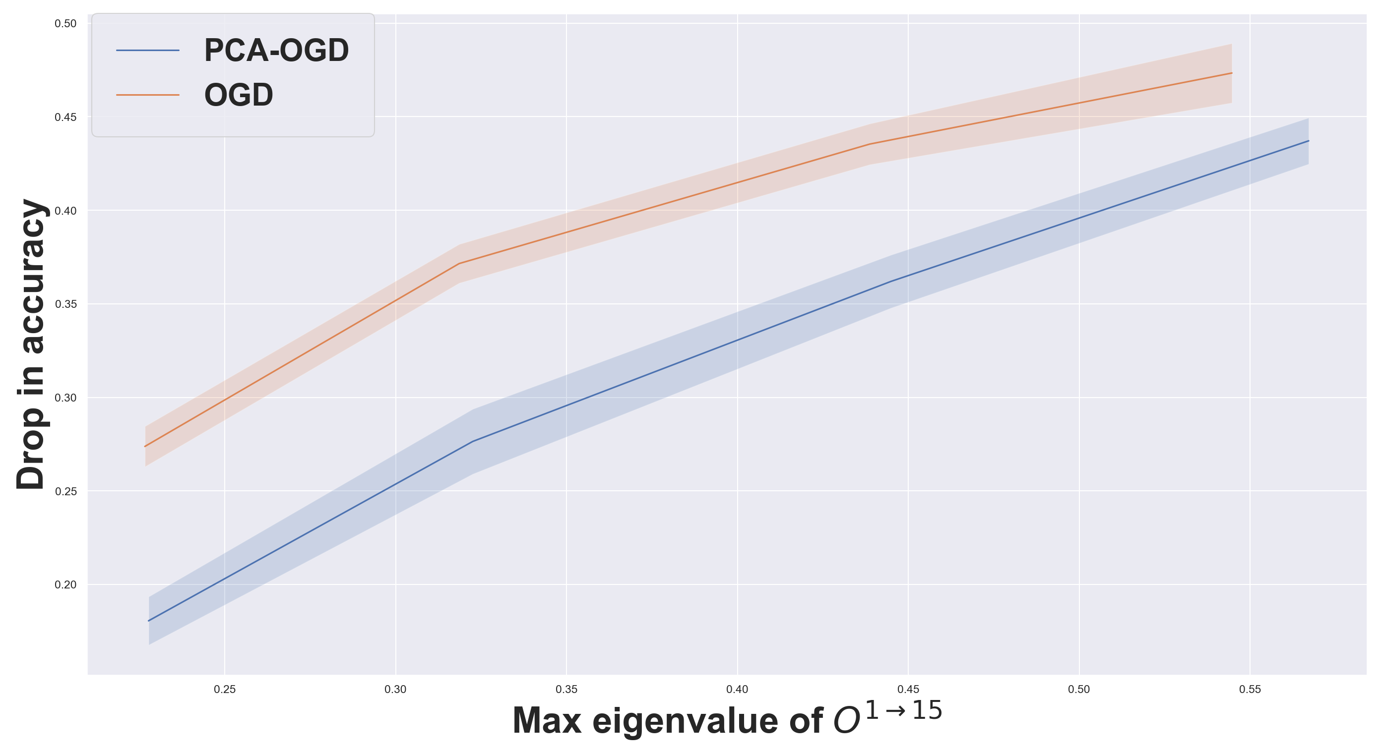
Figure 2: Drop in performance with respect to the maximum eigenvalue for Rotated MNIST (averaged over $5$ seeds $\pm 1$ std).

5.2 PCA-OGD reduces forgetting by efficiently leveraging structure in the data

Objective :

We show how capturing the top $d$ principal directions helps reducing Catastrophic Forgetting (Corollary 3).

Experiments :

We compare the spectrum of the NTK overlap matrix for different methods: SGD, GEM-NT, OGD and PCA-OGD, for different memory sizes.

Results:

We visualize the effect of the memory size on the forgetting through the eigenvalues of the NTK overlap matrix $O^{\tau_{S}\rightarrow\tau_{T}}$. To unclutter the plot, Figure 3 only shows the results for memory sizes of $25$ and $200$. Because PCA-OGD compresses the information in a few number of components, it has lower eigenvalues than both OGD and GEM-NT and the gap gets higher when increasing the memory size to $200$. Table 9 in the Appendix confirms those findings by seeing that with $200$ components one can already explain $90.71\%$ of the variance.

Finally, the eigenvalues of SGD are higher than those of projection methods since it does not perform any projection of the source or target task.

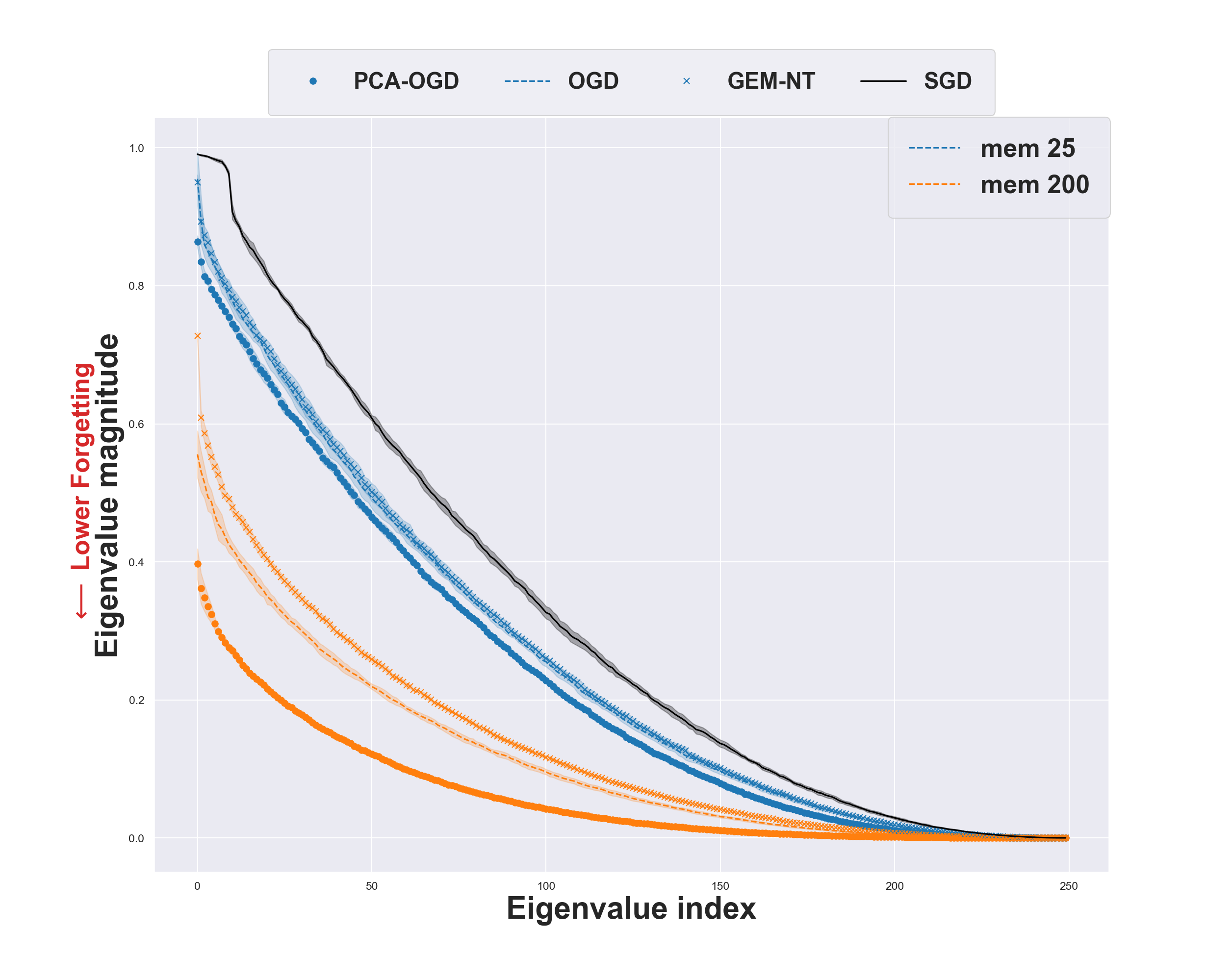
Figure 3: Comparison of the eigenvalues of $O^{1\rightarrow 2}$ on Rotated MNIST with increasing memory size. Lower values imply less forgetting (averaged over $5$ seeds $\pm 1$ std).

Finally, the final accuracies on Rotated and Permuted MNIST are reported in Figure 4 for the first seven tasks. In Rotated MNIST, we can see that PCA-OGD is twice more memory efficient than OGD: with a memory size of $100$ PCA-OGD has comparable results to OGD with a memory size $200$. Interestingly, while the marginal increase for PCA-OGD is roughly constant going from memory size $25$ to $50$ or $50$ to $100$, OGD incurs a high increase from memory size $100$ to $200$ while below that threshold the improvement is relatively small.

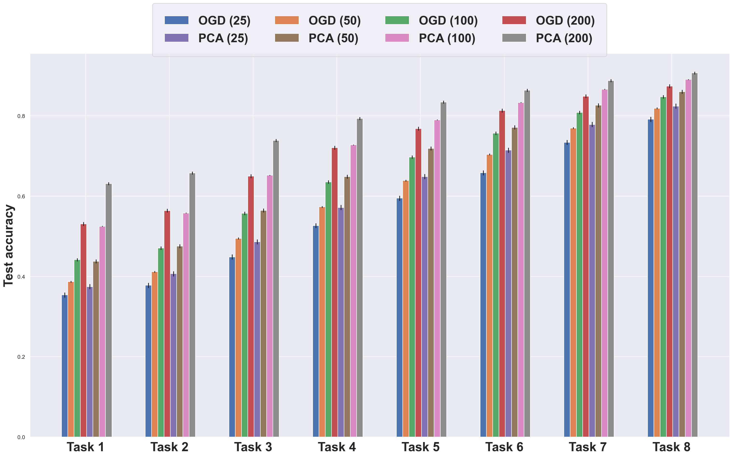
Figure 4: Final accuracy on Rotated MNIST for different memory size (averaged over $5$ seeds $\pm 1$ std). OGD needs twice as much memory as PCA-OGD in order to achieve the same performance (i.e compare OGD (200) and PCA (100).

We ran OGD and PCA-OGD on a counter-example dataset (Permuted MNIST), where there is no structure within the dataset (see Appendix 8.7). In this case, PCA-OGD is less efficient since it needs to keep more principal components than in a structured dataset setting.

5.3 General performance of PCA-OGD against baselines

Objective and Experiments :

We compare PCA-OGD against other baseline methods: SGD, A-GEM [Chaudhry et al., 2018] and OGD [Farajtabar et al., 2020]. Additionally to the final accuracies, we report the Average Accuracy $A_{T}$ and Forgetting Measure $F_{T}$ [Lopez-Paz and Ranzato, 2017, Chaudhry et al., 2018]. We run AGEM instead of GEM-NT which is faster with comparable results [Chaudhry et al., 2018] (since GEM-NT is solving a quadratic programming optimization at each iteration step). Definition of these metrics and full details of the experimental setup can be found in Appendix 8.11.

Results :

The results are summarized in Table 1 (additional results are presented in Appendix 8.11). Overall, PCA-OGD obtains comparable results to A-GEM. A-GEM has the advantage of accounting for the NTK changes by updating it while PCA-OGD and OGD are storing the gradients from previous iteration. The later therefore project updates orthogonally to outdated gradients. This issue has also been mentioned in [Bennani et al., 2020]. Note the good performance of PCA-OGD in Split CIFAR where the dataset size is $2,500$ (making the NTK assumption more realistic) and similar patterns are seen across tasks (CIFAR100 dataset is divided into $20$ superclasses within which we can count $5$ subfamilies hence having a pattern across tasks. To examine this hypothesis, we plot the NTK changes for different datasets in Appendix 8.10. We can indeed see that the NTK does not vary anymore after $1$ task for Split CIFAR while it increases linearly for MNIST datasets which confirms our hypothesis.

	SGD	EWC	A-GEM	OGD	PCA-OGD
	Permuted MNIST
$A_{T}$	76.81 $\pm$ 1.36	79.71 $\pm$ 0.52	83.4 $\pm$ 0.43	80.95 $\pm$ 0.5	81.44 $\pm$ 0.62
$F_{T}$	14.88 $\pm$ 1.64	3.81 $\pm$ 0.47	7.29 $\pm$ 0.45	9.72 $\pm$ 0.51	9.11 $\pm$ 0.65
	Rotated MNIST
$A_{T}$	66.07 $\pm$ 0.47	76.2 $\pm$ 0.62	83.52 $\pm$ 0.22	77.42 $\pm$ 0.35	82.05 $\pm$ 0.58
$F_{T}$	29.57 $\pm$ 0.56	13.44 $\pm$ 0.82	9.86 $\pm$ 0.28	16.52 $\pm$ 0.46	11.67 $\pm$ 0.65
	Split MNIST
$A_{T}$	95.1 $\pm$ 1.08	95.06 $\pm$ 1.15	94.25 $\pm$ 1.62	96.05 $\pm$ 0.34	95.96 $\pm$ 0.29
$F_{T}$	2.02 $\pm$ 1.48	2.08 $\pm$ 1.56	2.82 $\pm$ 1.72	0.37 $\pm$ 0.21	0.28 $\pm$ 0.15
	Split CIFAR
$A_{T}$	56.11 $\pm$ 1.65	65.45 $\pm$ 0.97	47.55 $\pm$ 2.4	69.77 $\pm$ 0.72	72.7 $\pm$ 0.97
$F_{T}$	22.69 $\pm$ 2.18	6.56 $\pm$ 1.49	31.36 $\pm$ 2.58	8.27 $\pm$ 0.31	5.39 $\pm$ 0.85

Table 1: Average Accuracy and Forgetting for all baselines considered across the datasets ($5$ seeds).

6 Conclusion

We present a theoretical analysis of CF in the NTK regime, for SGD and the projection based algorithms OGD, GEM-NT and PCA-OGD. We quantify the impact of the tasks similarity on CF through the NTK overlap matrix. Experiments support our findings that the overlap matrix is crucial in reducing CF and our proposed method PCA-OGD efficiently mitigates CF. However, our analysis relies on the core assumption of overparameterisation, an important next step is to account for the change of NTK over time. We hope this analysis opens new directions to study the properties of Catastrophic Forgetting for other Continual Learning algorithms.

7 Acknowledgments

The authors would like to thank Joelle Pineau for useful discussions and feedbacks. Finally, we thank Compute Canada for providing computational ressources used in this project.

8 Appendix

8.1 Proof of Lemma 1

For this proof, we will use the result of Thm. 1 from [Bennani et al., 2020] (particularly Remark 1) and notice that the expression of $f_{\tau_{T}}^{\star}$ can be espressed recursively with respect to $f_{\tau_{S}}^{\star}$:

Proof.

$$f_{\tau_{T}}^{\star}(x) =f_{\tau_{T}-1}^{\star}(x)+\langle\nabla_{\omega}f_{\tau_{T}-1}^{\star}(x),\omega_{\tau_{T}}^{\star}-\omega_{\tau_{T}-1}^{\star}\rangle$$

$$=f_{\tau_{T}-k}^{\star}(x)+...+\langle\nabla_{\omega}f_{\tau_{T}-2}^{\star}(x),\omega_{\tau_{T}-1}^{\star}-\omega_{\tau_{T}-2}^{\star}\rangle+\langle\nabla_{\omega}f_{\tau_{T}-1}^{\star}(x),\omega_{\tau_{T}}^{\star}-\omega_{\tau_{T}-1}^{\star}\rangle$$

$$=f_{\tau_{S}}^{\star}(x)+\sum_{k=\tau_{S}+1}^{\tau_{T}}\langle\nabla_{\omega}f_{k}^{\star}(x),\omega_{k}^{\star}-\omega_{k-1}^{\star}\rangle$$

$$=f_{\tau_{S}}^{\star}(x)+\sum_{k=\tau_{S}+1}^{\tau_{T}}\langle\nabla_{\omega}f_{0}(x),\omega_{k}^{\star}-\omega_{k-1}^{\star}\rangle\quad\text{(NTK constant)}$$

$$=f_{\tau_{S}}^{\star}(x)+\langle\nabla_{\omega}f_{0}(x),\omega_{\tau_{T}}^{\star}-\omega_{\tau_{S}}^{\star}\rangle$$

where we used constant NTK assumption, i.e $\nabla_{\omega}f_{\tau}^{\star}(x)=\nabla_{\omega_{0}}f(x)$ , $\forall\tau\in[T]$.

Using the fact that the kernel is given by $\phi(x)=\nabla_{w_{0}}f(x)$, we have that:

$$\delta^{\tau_{S}\rightarrow\tau_{T}}(X^{\tau_{S}}) =f_{\tau_{T}}^{\star}(X^{\tau_{S}})-f_{\tau_{S}}^{\star}(X^{\tau_{S}})$$

$$=\langle\phi(X^{\tau_{S}}),\omega_{\tau_{T}}^{\star}-\omega_{\tau_{S}}^{\star}\rangle$$

$$\Delta^{\tau_{S}\rightarrow\tau_{T}}(X^{\tau_{S}}) =\left\lVert\phi(X^{\tau_{S}})(\omega_{\tau_{T}}^{\star}-\omega_{\tau_{S}}^{\star})\right\rVert_{2}^{2}$$

This concludes the proof. ∎

8.2 Proof of Theorem 1

For this proof, we will decompose the drift from task $\tau_{S}$ to $\tau_{T}$ into a telescopic sum. We will then use SVD to factorize the expression of $(\omega_{\tau}^{\star}-\omega_{\tau-1}^{\star})$ and get the upper bound showed.

Proof.

$$\Delta^{\tau_{S}\rightarrow\tau_{T}}(X^{\tau_{S}}) =\left\lVert\phi(X^{\tau_{S}})(\omega_{\tau_{T}}^{\star}-\omega_{\tau_{S}}^{\star})\right\rVert_{2}^{2}\quad(\text{Lemma~{}\ref{lemma:def_forgetting}})$$ (13)

$$=\left\lVert\sum_{k=\tau_{S}+1}^{\tau_{T}}\phi(X^{\tau_{S}})(\omega_{k}^{\star}-\omega_{k-1}^{\star})\right\rVert_{2}^{2}$$ (14)

$$=\left\lVert\sum_{k=\tau_{S}+1}^{\tau_{T}}\phi(X^{\tau_{S}})\underbrace{\phi(X^{k})^{\top}[\phi(X^{k})\phi(X^{k})^{\top}+\lambda I_{n_{k}}]^{-1}\tilde{y}_{k}}_{\text{from Thm. 1 of \cite[citep]{[\@@bibref{AuthorsPhrase1Year}{bennani2020generalisation}{\@@citephrase{, }}{}]}}}\right\rVert_{2}^{2}$$ (15)

$$=\left\lVert\sum_{k=\tau_{S}+1}^{\tau_{T}}U_{\tau_{S}}\Sigma_{\tau_{S}}V_{\tau_{S}}^{\top}V_{k}\Sigma_{k}U_{k}^{\top}[U_{k}\Sigma_{k}^{2}U_{k}^{\top}+\lambda I_{n_{k}}]^{-1}\tilde{y}_{k}\right\rVert_{2}^{2}\quad(\text{SVD})$$ (16)

$$=\left\lVert\sum_{k=\tau_{S}+1}^{\tau_{T}}U_{\tau_{S}}\Sigma_{\tau_{S}}\underbrace{V_{\tau_{S}}^{\top}V_{k}}_{O^{\tau_{S}\rightarrow k}_{SGD}}\underbrace{\Sigma_{k}[\Sigma_{k}^{2}+\lambda I_{n_{k}}]^{-1}U_{k}^{\top}}_{M_{k}}\tilde{y}_{k}\right\rVert_{2}^{2}$$ (17)

Where we used the SVD $\phi(X^{\tau})=U_{\tau}\Sigma_{\tau}V_{\tau}^{T},\forall\tau\in[T]$. This concludes the proof. ∎

8.3 Proof of Corolary 1

For this proof, we will bound the Catastrophic Forgetting as a function of the principal angles between the source and target subspaces. Indeed, given two subspace $\tau_{S}$ and $\tau_{T}$ represented by their orthonormal basis concatenated respectively in $V_{\tau_{S}}$ and $V_{\tau_{T}}$, the elements of the diagonal matrix $\Theta^{\tau_{S}\rightarrow\tau_{T}}$ resulting from the SVD of $V_{\tau_{S}}^{\top}V_{\tau_{T}}$ are the cosines of the principal angles between these two subspace [Wedin, 1983, Zhu and Knyazev, 2013].

Proof.

$$\Delta^{\tau_{S}\rightarrow\tau_{T}}(X^{\tau_{S}}) \leq\sum_{k=\tau_{S}+1}^{\tau_{T}}\left\lVert U_{\tau_{S}}\Sigma_{\tau_{S}}V_{\tau_{S}}^{\top}V_{k}\Sigma_{k}[\Sigma_{k}^{2}+\lambda I_{n_{k}}]^{-1}U_{k}^{\top}\tilde{y}_{k}\right\rVert_{2}^{2}$$ (19)

$$\leq\sum_{k=\tau_{S}+1}^{\tau_{T}}\left\lVert U_{\tau_{S}}\Sigma_{\tau_{S}}\right\rVert_{2}^{2}\left\lVert V_{\tau_{S}}^{\top}V_{k}\right\rVert_{2}^{2}\left\lVert\Sigma_{k}[\Sigma_{k}^{2}+\lambda I_{n_{k}}]^{-1}U_{k}^{\top}\tilde{y}_{k}\right\rVert_{2}^{2}\quad(\text{sub-multiplicativity of norm 2})$$ (20)

$$\leq\sum_{k=\tau_{S}+1}^{\tau_{T}}\left\lVert\Sigma_{\tau_{S}}\right\rVert_{2}^{2}\left\lVert V_{\tau_{S}}^{\top}V_{k}\right\rVert_{2}^{2}\left\lVert M_{k}\tilde{y}_{k}\right\rVert_{2}^{2}\quad\quad(U_{\tau_{S}}\text{ is an orthonormal matrix})$$ (21)

$$\leq\sigma_{\tau_{S},1}^{2}\sum_{k=\tau_{S}+1}^{\tau_{T}}\left\lVert Y\Theta^{\tau_{S}\rightarrow k}Z^{\top}\right\rVert_{2}^{2}\left\lVert M_{k}\tilde{y}_{k}\right\rVert_{2}^{2}\quad\quad(\text{SVD})$$ (22)

$$\leq\sigma_{\tau_{S},1}^{2}\sum_{k=\tau_{S}+1}^{\tau_{T}}\left\lVert\Theta^{\tau_{S}\rightarrow k}\right\rVert_{2}^{2}\left\lVert M_{k}\tilde{y}_{k}\right\rVert_{2}^{2}\quad\quad(Y,Z\text{ are orthonormal matrices})$$ (23)

where $Y\Theta^{\tau_{S}\rightarrow k}Z^{\top}$ is the SVD of $V_{\tau_{S}}^{\top}V_{k}$. This concludes the proof. ∎

8.4 Proof of Corollary 2

We first need to prove a corollary that is exactly the same as Corollary 4 (shown below), the difference lies in the kernel definition. Under the same notation as in Corollary 4, the solution after training on task $\tau$ for GEM-NT is such that:

$$\omega_{\tau}^{\star}-\omega_{\tau-1}^{\star}=\overline{\phi}_{\tau}(X^{\tau})^{\top}(\kappa_{\tau}(X^{\tau},X^{\tau})+\lambda I_{n_{\tau}})^{-1}\tilde{y}_{\tau}$$ (25)

where:

$$\kappa_{\tau}(x,x^{\prime}) =\overline{\phi}_{\tau}(x)\overline{\phi}_{\tau}(x^{\prime})^{\top},$$

$$\overline{\phi}_{\tau}(x) =\phi(x)T_{\tau-1},$$

$$T_{\tau} =I_{p}-G_{\tau}(G_{\tau})^{\top},$$

$$\tilde{y}_{\tau} =y_{\tau}-y_{\tau-1\rightarrow\tau},$$

$$y_{\tau-1\rightarrow\tau} =f_{\tau-1}^{\star}(X^{\tau}),$$

Proof.

of Corollary 2 Similarly to Proof of Theorem 1:

$$\Delta^{\tau_{S}\rightarrow\tau_{T}}(X^{\tau_{S}}) =\left\lVert\phi(X^{\tau_{S}})(\omega_{\tau_{T}}^{\star}-\omega_{\tau_{S}}^{\star})\right\rVert_{2}^{2}\quad(\text{Lemma~{}\ref{lemma:def_forgetting}})$$ (26)

$$=\left\lVert\sum_{k=\tau_{S}+1}^{\tau_{T}}\phi(X^{\tau_{S}})(\omega_{k}^{\star}-\omega_{k-1}^{\star})\right\rVert_{2}^{2}$$ (27)

$$=\left\lVert\sum_{k=\tau_{S}+1}^{\tau_{T}}\phi(X^{\tau_{S}})\underbrace{\overline{\phi}(X^{k})^{\top}[\overline{\phi}(X^{k})\overline{\phi}(X^{k})^{\top}+\lambda I_{n_{k}}]^{-1}\overline{y}_{k}}_{\text{as shown above}}\right\rVert_{2}^{2}$$ (28)

$$=\left\lVert\sum_{k=\tau_{S}+1}^{\tau_{T}}U_{\tau_{S}}\Sigma_{\tau_{S}}V_{\tau_{S}}^{\top}T_{k-1}^{\top}V_{k}\Sigma_{k}U_{k}^{\top}[\overline{\phi}(X^{k})\overline{\phi}(X^{k})^{\top}+\lambda I_{n_{k}}]^{-1}\overline{y}_{k}\right\rVert_{2}^{2}\quad(\text{SVD})$$ (29)

$$=\left\lVert\sum_{k=\tau_{S}+1}^{\tau_{T}}U_{\tau_{S}}\Sigma_{\tau_{S}}\underbrace{V_{\tau_{S}}^{\top}T_{k-1}T_{k-1}^{\top}V_{k}}_{O^{\tau_{S}\rightarrow k}_{\text{GEM-NT}}}\underbrace{\Sigma_{k}U_{k}^{\top}[\overline{\phi}(X^{k})\overline{\phi}(X^{k})^{\top}+\lambda I_{n_{k}}]^{-1}}_{M_{k}}\overline{y}_{k}\right\rVert_{2}^{2}\quad(T_{k-1})^{n}=T_{k-1},\forall n\geq 1$$ (30)

This concludes the proof. ∎

8.5 Forgetting for PCA-OGD

To prove the forgetting expression for PCA-OGD, we will use a corollary arising naturally from Theorem 1 of [Bennani et al., 2020] which extends the expression of the learned weights $(\omega_{\tau+1}^{\star}-\omega_{\tau}^{\star})$ from the infinite to the finite memory case. The proof will be shown after the proof of Corollary 3 for the flow of the understanding.

Corollary 4 (Convergence of PCA-OGD under finite memory).

Given $\mbox{$\mathcal{T}$}_{1},...,\mbox{$\mathcal{T}$}_{T}$ a sequence of tasks. If the learning rate satisfies: $\eta_{\tau}<\frac{1}{\left\lVert\kappa_{\tau}(X^{\tau},X^{\tau})+\lambda I_{n_{\tau}}\right\rVert}$, $\kappa_{\tau},\forall\tau\in[T]$ is invertible with a weight decay regularizer $\lambda>0$, the solution after training on task $\tau$ is such that:

$$\omega_{\tau}^{\star}-\omega_{\tau-1}^{\star}=\tilde{\phi}_{\tau}(X^{\tau})^{\top}(\kappa_{\tau}(X^{\tau},X^{\tau})+\lambda I_{n_{\tau}})^{-1}\tilde{y}_{\tau}$$ (32)

where:

$$\kappa_{\tau}(x,x^{\prime}) =\tilde{\phi}_{\tau}(x)\tilde{\phi}_{\tau}(x^{\prime})^{\top},$$

$$\tilde{\phi}_{\tau}(x) =\phi(x)T_{\tau-1,:d},$$

$$T_{\tau,:d} =I_{p}-P_{\tau,:d}P_{\tau,:d}^{\top},$$

$$\phi(x) =\nabla_{\omega_{0}}f_{0}^{\star}(x),$$

$$\tilde{y}_{\tau} =y_{\tau}-y_{\tau-1\rightarrow\tau},$$

$$y_{\tau-1\rightarrow\tau} =f_{\tau-1}^{\star}(X^{\tau}),$$

where $T_{0,:d}=I_{p}$ since there are no previous task when training on task $1$.

Proof.

of Corollary 3

Similarly to Proof of Theorem 1:

$$\Delta^{\tau_{S}\rightarrow\tau_{T}}(X^{\tau_{S}}) =\left\lVert\phi(X^{\tau_{S}})(\omega_{\tau_{T}}^{\star}-\omega_{\tau_{S}}^{\star})\right\rVert_{2}^{2}\quad(\text{Lemma~{}\ref{lemma:def_forgetting}})$$ (33)

$$=\left\lVert\sum_{k=\tau_{S}+1}^{\tau_{T}}\phi(X^{\tau_{S}})(\omega_{k}^{\star}-\omega_{k-1}^{\star})\right\rVert_{2}^{2}$$ (34)

$$=\left\lVert\sum_{k=\tau_{S}+1}^{\tau_{T}}\phi(X^{\tau_{S}})\underbrace{\tilde{\phi}(X^{k})^{\top}[\tilde{\phi}(X^{k})\tilde{\phi}(X^{k})^{\top}+\lambda I_{n_{k}}]^{-1}\tilde{y}_{k}}_{\text{from Corollary~{}\ref{cor:convergence_pca_finite_case} }}\right\rVert_{2}^{2}$$ (35)

$$=\left\lVert\sum_{k=\tau_{S}+1}^{\tau_{T}}U_{\tau_{S}}\Sigma_{\tau_{S}}V_{\tau_{S}}^{\top}T_{k-1,:d}^{\top}V_{k}\Sigma_{k}U_{k}^{\top}[\tilde{\phi}(X^{k})\tilde{\phi}(X^{k})^{\top}+\lambda I_{n_{k}}]^{-1}\tilde{y}_{k}\right\rVert_{2}^{2}\quad(\text{SVD})$$ (36)

$$=\left\lVert\sum_{k=\tau_{S}+1}^{\tau_{T}}U_{\tau_{S}}\Sigma_{\tau_{S}}\underbrace{V_{\tau_{S}}^{\top}R_{k-1,d:}R_{k-1,d:}^{\top}V_{k}}_{O^{\tau_{S}\rightarrow k}_{PCA}}\Sigma_{k}\underbrace{U_{k}^{\top}[\tilde{\phi}(X^{k})\tilde{\phi}(X^{k})^{\top}+\lambda I_{n_{k}}]^{-1}}_{M_{k}}\tilde{y}_{k}\right\rVert_{2}^{2}$$ (37)

∎

Proof of Corollary 4.

In the same fashion as [Bennani et al., 2020], we prove Corollary 4 by induction. Our induction hypothesis $$H_{\tau} \mathcal{H}_{\tau} k\leq\tau$$ is the following : : For all , Corollary 4 holds.

First, we prove that $$\mathcal{H}_{1}$$ holds.

The proof is straightforward. For the first task, since there were no previous tasks, PCA-OGD on this task is the same as SGD.

Therefore, it is equivalent to minimising the following objective :

$$\operatorname*{arg\,min}_{\omega\in\mathbb{R}^{p}} \left\lVert f_{0}(X^{1})+\phi(X^{1})(\omega-\omega_{0}^{\star})-y_{1}\right\rVert_{2}^{2}+\frac{1}{2}\lambda\left\lVert\omega-\omega_{0}\right\rVert_{2}^{2}$$

where $$\phi(x)=\nabla_{\omega_{0}^{\star}}f_{0}^{\star}(x)$$.

Substituing the residual term $$\tilde{y}_{1}=y_{1}-f_{0}(X^{1})$$, we get:

$$\operatorname*{arg\,min}_{\omega\in\mathbb{R}^{p}} \left\lVert\phi(X^{1})(\omega-\omega_{0}^{\star})-\tilde{y}_{1}\right\rVert_{2}^{2}+\frac{1}{2}\lambda\left\lVert\omega-\omega_{0}\right\rVert_{2}^{2}$$

The objective is quadratic and the Hessian is positive definite, therefore the minimum exists and is unique

$$\omega_{1}^{\star}-\omega_{0}^{\star} =\phi(X^{1})^{\top}(\phi(X^{1})\phi(X^{1})^{\top}+\lambda I_{n_{1}})^{-1}\tilde{y}_{1}$$

Under the NTK regime assumption :

$$f_{1}^{\star}(x) =f_{0}^{\star}(x)+\nabla_{\omega_{0}}f_{0}^{\star}(x)^{\top}(\omega_{1}^{\star}-\omega_{0}^{\star})$$

Then, by replacing into $$\omega_{1}^{\star}-\omega_{0}^{\star}$$ :

$$f_{1}^{\star}(x) =f_{0}^{\star}(x)+\nabla_{\omega_{0}}f_{0}^{\star}(x)\phi(X^{1})^{\top}(\phi(X^{1})\phi(X^{1})^{\top}+\lambda I_{n_{1}})^{-1}\tilde{y}_{1}$$

$$f_{1}^{\star}(x) =f_{0}^{\star}(x)+\kappa_{1}(x,X^{1})(\kappa_{1}(X^{1},X^{1})+\lambda I_{n_{1}})^{-1}\tilde{y}_{1}$$

Finally :

$$f_{1}^{\star}(x)-f_{0}^{\star}(x) =\kappa_{1}(x,X^{1})(\kappa_{1}(X^{1},X^{1})+\lambda I_{n_{1}})^{-1}\tilde{y}_{1}$$

Where :

$$\kappa_{1}(X^{1},X^{1}) =\tilde{\phi_{1}}(X^{1})\tilde{\phi}_{1}(X^{1})^{\top}$$

$$=\phi(X^{1})T_{0,:d}T_{0,:d}^{\top}\phi(X^{1})^{\top}$$

$$=\phi(X^{1})\phi(X^{1})^{\top}$$

Since there is no previous task and $$T_{0,:d} T_{0,:d}=I_{p} \tilde{y}_{1}=y_{1}$$ contains no eigenvectors yet, we have and .

This completes the proof of $$\mathcal{H}_{1}$$.

Let $$\tau\in\mathcal{N}^{\star} \mathcal{H}_{\tau} \mathcal{H}_{\tau+1}$$, we assume that is true, then we show that is true.

At the end of training of task $$\tau d \phi(X^{\tau})\phi(X^{\tau})^{\top} P_{\tau-1,:d}\in\mathbb{R}^{p\times(\tau-1)\cdot d} P_{\tau,:d}\in\mathbb{R}^{p\times\tau\cdot d}$$, we add the first eigenvectors of to to form the matrix through PCA decomposition

.

The update during the training of task $$\tau+1 d 1 \tau T_{\tau,:d}$$ is projected orthogonally to the first components of task until via the matrix :

$$\omega_{\tau+1}(t+1) =\omega_{\tau}^{\star}-\eta T_{\tau,:d}\nabla_{\omega}\mathcal{L}^{\tau}_{\lambda}(\omega_{\tau+1}(t))$$

$$\omega_{\tau+1}(t+1)-\omega_{\tau}^{\star} =-\eta T_{\tau,:d}\nabla_{\omega}\mathcal{L}^{\tau}_{\lambda}(\omega_{\tau+1}(t))$$

$$\omega_{\tau+1}(t+1)-\omega_{\tau}^{\star} =T_{\tau,:d}\tilde{\omega}_{\tau+1}$$

Where $$\eta T_{\tau,:d}=I_{p}-P_{\tau,:d}P_{\tau,:d}^{\top}$$ is the learning rate and .

We rewrite the objective by plugging in the variables we just defined. The two objectives are equivalent :

$$\operatorname*{arg\,min}_{\tilde{\omega}_{\tau+1}\in\mathbb{R}^{p}} \left\lVert\underbrace{\phi(X^{\tau+1})T_{\tau,:d}}_{\phi_{\tau+1}(X^{\tau+1})}\tilde{w}_{\tau+1}-\tilde{y}_{\tau+1}\right\rVert_{2}^{2}$$

The optimisation objective is quadratic, unconstrainted, with a positive definite hessian. Therefore, an optimum exists and is unique :

$$\tilde{\omega}^{\star}_{\tau+1} =\phi_{\tau+1}(X^{\tau+1})^{\top}(\phi_{\tau+1}(X^{\tau+1})\phi_{\tau+1}(X^{\tau+1})^{\top})^{-1}\tilde{y}_{\tau+1}$$

$$\omega_{\tau+1}^{\star}-\omega_{\tau}^{\star} =\phi_{\tau+1}(X^{\tau+1})^{\top}(\phi_{\tau+1}(X^{\tau+1})\phi_{\tau+1}(X^{\tau+1})^{\top})^{-1}\tilde{y}_{\tau+1}$$

$$\omega_{\tau+1}^{\star}-\omega_{\tau}^{\star} =\phi_{\tau+1}(X^{\tau+1})^{\top}(\kappa_{\tau+1}(X^{\tau+1},X^{\tau+1}))^{-1}\tilde{y}_{\tau+1}$$

Recall from the induction hypothesis of $$\mathcal{H}_{\tau} f_{\tau}^{\star}(x)$$ the general form of :

$$f_{\tau}^{\star}(x) =f_{\tau-1}^{\star}(x)+\langle\nabla_{\omega_{0}}f_{0}^{\star}(x),\omega_{\tau+1}^{\star}-\omega_{\tau}^{\star}\rangle$$

After training on task $$\tau+1$$ :

$$f_{\tau+1}^{\star}(x) =f_{\tau-1}^{\star}(x)+\langle\nabla_{\omega_{0}}f_{0}^{\star}(x),\omega_{\tau+1}^{\star}-\omega_{\tau-1}^{\star}\rangle$$

$$f_{\tau+1}^{\star}(x) =f_{\tau-1}^{\star}(x)+\langle\nabla_{\omega_{0}}f_{0}^{\star}(x),\omega_{\tau+1}^{\star}-\omega_{\tau-1}^{\star}+\underbrace{\omega_{\tau}^{\star}-\omega_{\tau}^{\star}}_{=0}\rangle$$

$$f_{\tau+1}^{\star}(x) =\underbrace{f_{\tau-1}^{\star}(x)+\langle\nabla_{\omega_{0}}f_{0}^{\star}(x),\omega_{\tau}^{\star}-\omega_{\tau-1}^{\star}\rangle}_{f_{\tau}^{\star}(x)}+\langle\nabla_{\omega_{0}}f_{0}^{\star}(x),\omega_{\tau+1}^{\star}-\omega_{\tau}^{\star}\rangle$$

$$f_{\tau+1}^{\star}(x) =f_{\tau}^{\star}(x)+\langle\nabla_{\omega_{0}}f_{0}^{\star}(x),\omega_{\tau+1}^{\star}-\omega_{\tau}^{\star}\rangle$$

$$f_{\tau+1}^{\star}(x) =f_{\tau}^{\star}(x)+\phi(x)\phi_{\tau+1}(X^{\tau+1})^{\top}(\kappa_{\tau+1}(X^{\tau+1},X^{\tau+1}))^{-1}\tilde{y}_{\tau+1}$$

$$f_{\tau+1}^{\star}(x) =f_{\tau}^{\star}(x)+\phi(x)T_{\tau,:d}^{\top}\phi_{\tau+1}(X^{\tau+1})^{\top}(\kappa_{\tau+1}(X^{\tau+1},X^{\tau+1}))^{-1}\tilde{y}_{\tau+1}$$

$$f_{\tau+1}^{\star}(x) =f_{\tau}^{\star}(x)+\underbrace{\phi(x)T_{\tau,:d}T_{\tau,:d}^{\top}\phi_{\tau+1}(X^{\tau+1})^{\top}}_{\kappa_{\tau+1}(x,X^{\tau+1})}(\kappa_{\tau+1}(X^{\tau+1},X^{\tau+1}))^{-1}\tilde{y}_{\tau+1}\quad(\text{ since }(T_{\tau,:d})^{\top}=T_{\tau,:d})$$

$$f_{\tau+1}^{\star}(x) =f_{\tau}^{\star}(x)+\kappa_{\tau+1}(x,X^{\tau+1})(\kappa_{\tau+1}(X^{\tau+1},X^{\tau+1}))^{-1}\tilde{y}_{\tau+1}$$

We have proven $$\mathcal{H}_{t+1}$$ and conclude the proof of Corollary 4.

∎

8.6 Algorithms summary

Properties	$O^{\tau_{S}\rightarrow\tau_{T}}_{X}$	$X$	Elements stored	Recompute
	$=V_{\tau_{S}}^{\top}\mathbf{XX}^{\top}V_{\tau_{T}}$	contains	in the memory	NTK?
SGD	X=$I_{\tau_{S}}$	NA	NA	NA
GEM-NT	X=$\mathbf{\overline{G}_{\tau_{T}-1}}$	samples of $\nabla\mathcal{L}(X^{\tau})$	samples of $X^{\tau}$	Yes
OGD	X=$\mathbf{R_{\tau_{T}-1}}$	samples of $\nabla f(X^{\tau})$	samples of $\nabla f(X^{\tau})$	No
PCA-OGD	X=$\mathbf{R_{\tau_{T}-1,:d}}$	top eigenvectors of $\nabla f(X^{\tau})$	top eigenvectors of $\nabla f(X^{\tau})$	No

Table 2: Property of the Overlap matrix for each method which is responsible for mitigating Catastrophic Forgetting. NA: Not applicable

NTK overlap matrix

First of all, the three methods GEM-NT, OGD, PCA-OGD differs from SGD by the the matrix $X$ (1st column) that contains either the features map $\nabla_{\omega}f(x)$ or the gradient loss function.

Elements stored

GEM-NT and OGD both samples random elements at the end of each task $\tau$ to store in the memory. For the sake of understanding, if we assume a mean square loss function, with a batch size equal to one, the gradient loss function becomes: $g_{\tau}^{\text{(GEM-NT)}}=\underbrace{\nabla_{\omega}f_{\tau}(x)}_{g_{\tau}^{(\text{OGD})}}(f_{\tau}(x)-y_{\tau})$. From here, we see that GEM-NT weights the features maps by the residual of a given task $k<\tau$ when training on task $\tau$.

Information compression

PCA-OGD compresses the information contained in the data by storing the principal components of $\nabla_{\omega}f(X^{\tau})$ through PCA. If the data has structure such as Rotated MNIST or Split CIFAR (See Section 9), storing few components will explain a high percentage of variance of the data of component in order to explain the dataset variance.

Accounting for the NTK variation

The drawback OGD and PCA-OGD compared to GEM-NT is that the NTK is assumed to be constant which is not always the case in practice (See Section 8.10). PCA-OGD and OGD will then project orthogonally to a vector that is outdated.

8.7 The counter-example of Permuted MNIST: no structure

We now examine the dataset Permuted MNIST and try to understand why PCA-OGD is not efficient in such case. Each task is an MNIST dataset where a different and uniform permutation of pixels is applied. This has the particularity of removing any extra-task correlations and patterns.

Eigenvalues of the NTK overlap matrix :

Figure 5(a) shows the eigenvalues of the NTK overlap matrix when increasing buffer size. First of all, we notice that the magnitude of the eigenvalues is very small compared to Figure 3. This is explained by the fact that each task shares almost no correlations, meaning that the cosine of angle of the two subspaces might be close to 0 (small eigenvalues). Additionally, we see that increasing the memory size does not reduce much the eigenvalue magnitude. This is due to the distribution of eigenvalues (See Figure 9) which are spread more uniformly than Permuted MNIST and Split CIFAR, meaning that more components need to be kept in order to explain a high $\%$ of the variance. In this situation, PCA-OGD does not have much advantage compared to OGD (See also toy example, Supplementary Material Section 8.12).

Final accuracy with OGD :

We now compare final performance against OGD (See Figure 5(b)). PCA-OGD does sensitively well compared to OGD (except for the first task where performance are much worse). This can be explained by the fact that PCA-OGD needs to keep a lot of components to explain a high percentage of variance such that selecting random element like OGD will results in comparable results. This is all the more confirmed by Table 3, keeping $50$ components only explains $50\%$ of the variance while it respectively explains $81\%$ for Rotated MNIST and $72\%$ for Split CIFAR. As mentionned by [Farquhar and Gal, 2018], even though such datasets meets the definition of CL, it is an irrealistic setting since “new situations look confusingly similar to old ones’ ”. Hence methods that leverage structure like PCA-OGD can be useful.

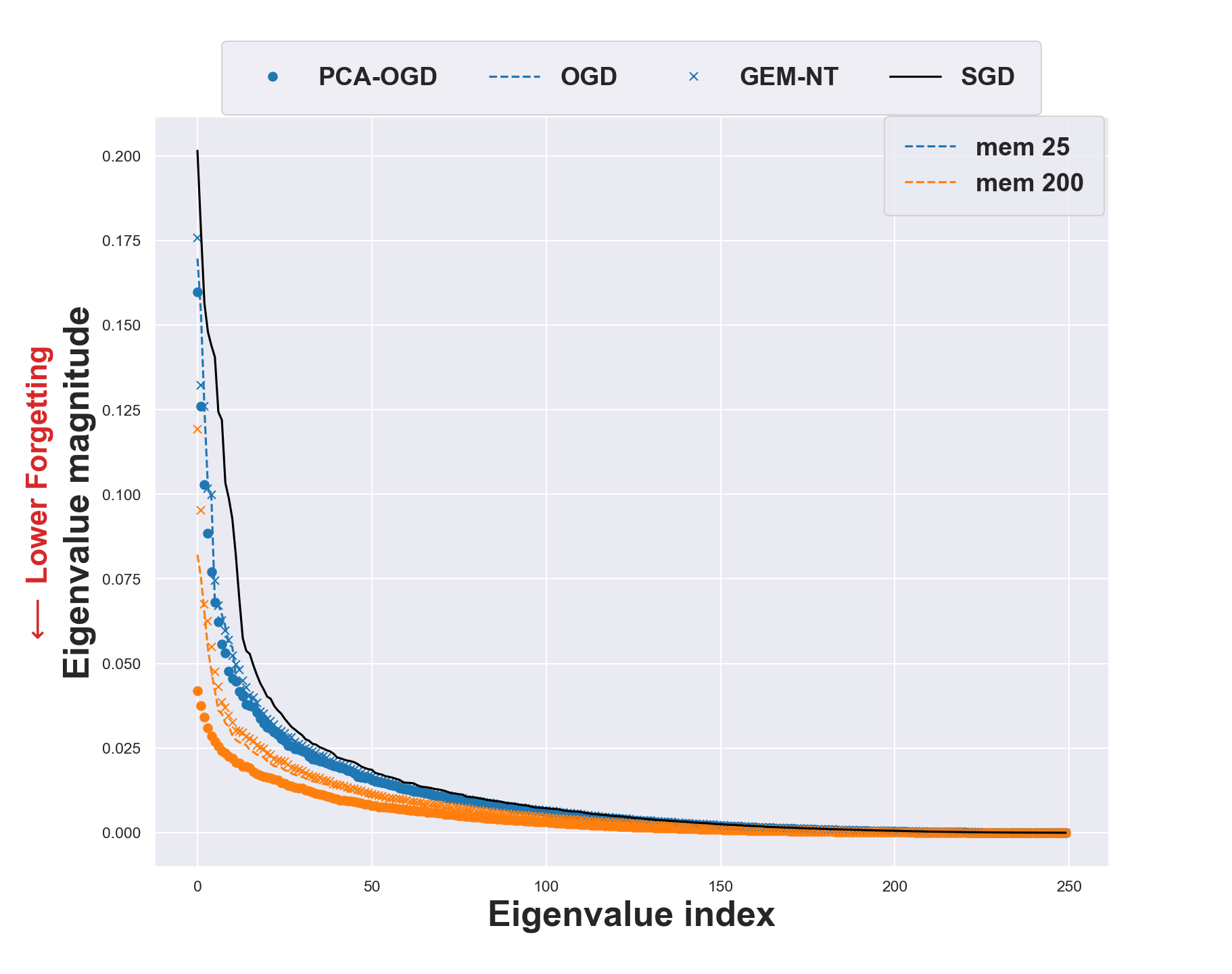
(a)

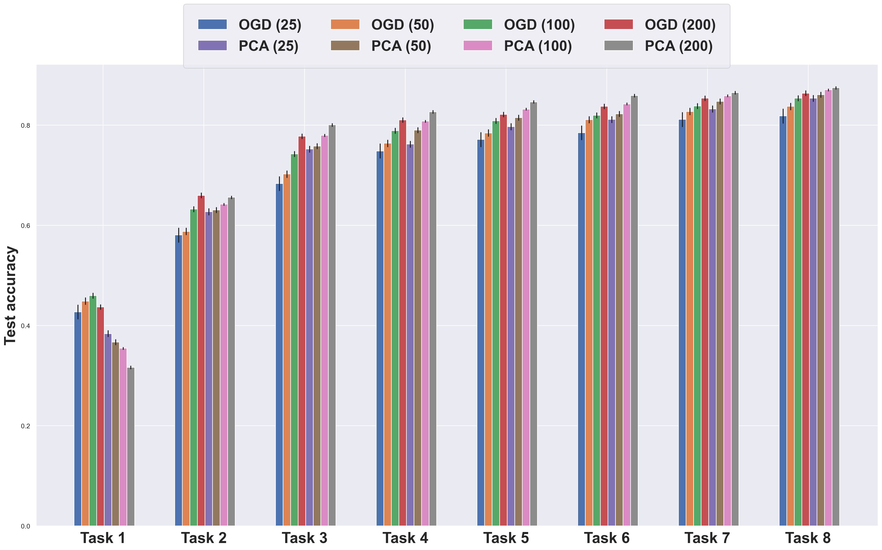
(b)

8.8 Comparison PCA-OGD versus OGD

Figure 6: Final accuracy on Rotated MNIST for different memory size (averaged over $5$ seeds $\pm 1$ std). OGD needs twice as much memory as PCA-OGD in order to achieve the same performance (i.e compare OGD (200) and PCA (100).

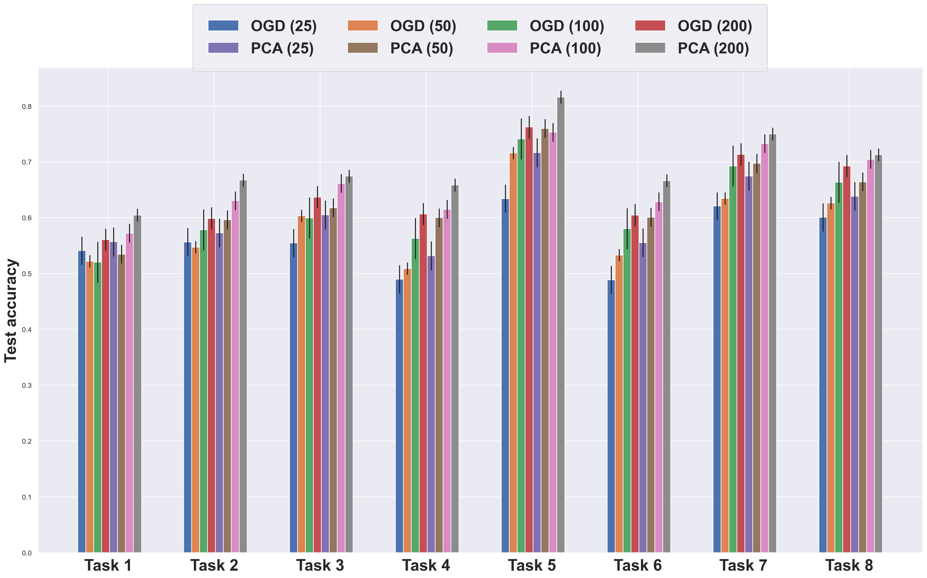
Figure 7: Final accuracy on Split CIFAR for different memory size (averaged over $5$ seeds $\pm 1$ std). When dataset is well structured PCA-OGD efficiently leverages the pattern (i.e compare OGD (200) and PCA (100).

Figure 8: Final accuracy on Permuted MNIST for different memory size. When there is no structure, information captured by PCA-OGD from previous tasks cannot be leveraged for future tasks. OGD and PCA-OGD have comparable performance (except for the first task).

8.9 Structure in the data

We sample a subset of $s=3,000$ samples from different datasets $x^{\tau}_{j}$,$j=1,...,3000$ (Permuted and Rotated MNIST), then we perform PCA on $\phi(x^{\tau}_{j})\phi(x^{\tau}_{j})^{\top}$ and keep the $d$ top components. Having a total memory size of $M=200,500,1000,2000,3000$ and training on $15$ tasks means that each task will be allocated $M/14$ since we omit the last task. As seen in Figure 9 for a total memory size of $200$, we only keep $14$ components which corresponds to $38.84\%$ of the variance explained in Permuted MNIST while it represents $71.06\%$ for Rotated MNIST. This is naturally explained by the fact that having random permutations breaks the structure of the data and in order to keep the most information would we need to allocate a large amount of memory.

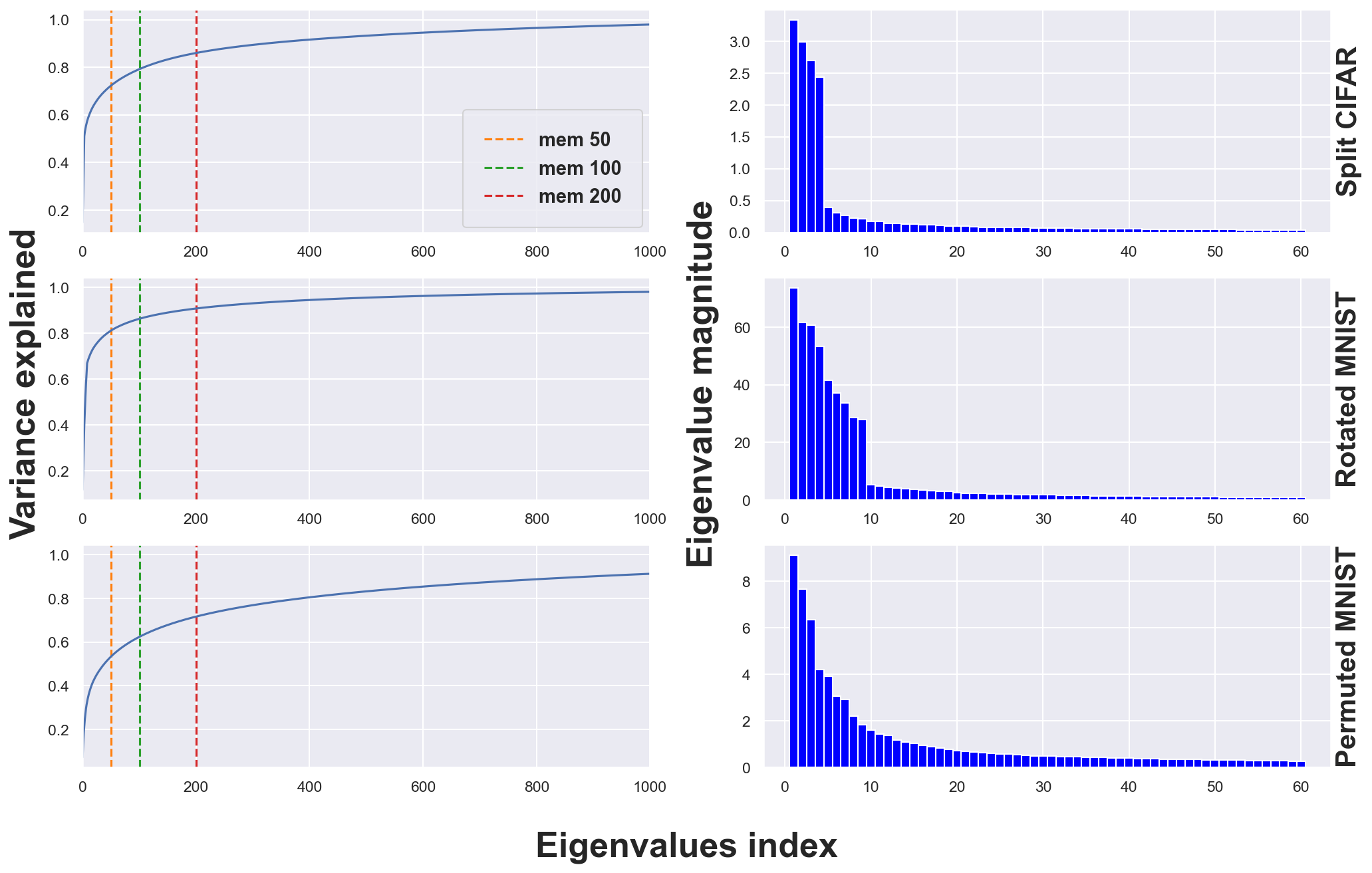
Figure 9: Percentage of variance explained for different datasets. Verticale lines on the left represents the number of components kept or the memory allocated per task. We have truncated the x-axis to focus on the interesting part.

components kept	Permuted MNIST	Rotated MNIST	Split CIFAR
10	35.13	68.52	58.87
25	45.14	75.54	65.99
50	53.33	81.09	72.27
100	62.37	86.23	79.19
200	71.65	90.71	85.99
500	83.20	94.42	93.24

Table 3: Percentage of variance explained with different memory size when performing PCA on $s=3,000$ samples (except for Split CIFAR where $s=1,500$).

8.10 NTK changes

We measure the change in NTK of PCA-OGD from its initialization value for different dataset size for a fixed architecture after each task (See Figure 10). The green curve shows the actual parameters used for the experiments. Although, there is linear increase of the NTK for MNIST datasets, it is approximately constant (after the first task) for Split CIFAR which validates the constant NTK assumption and explains the good result of PCA-OGD for this dataset.

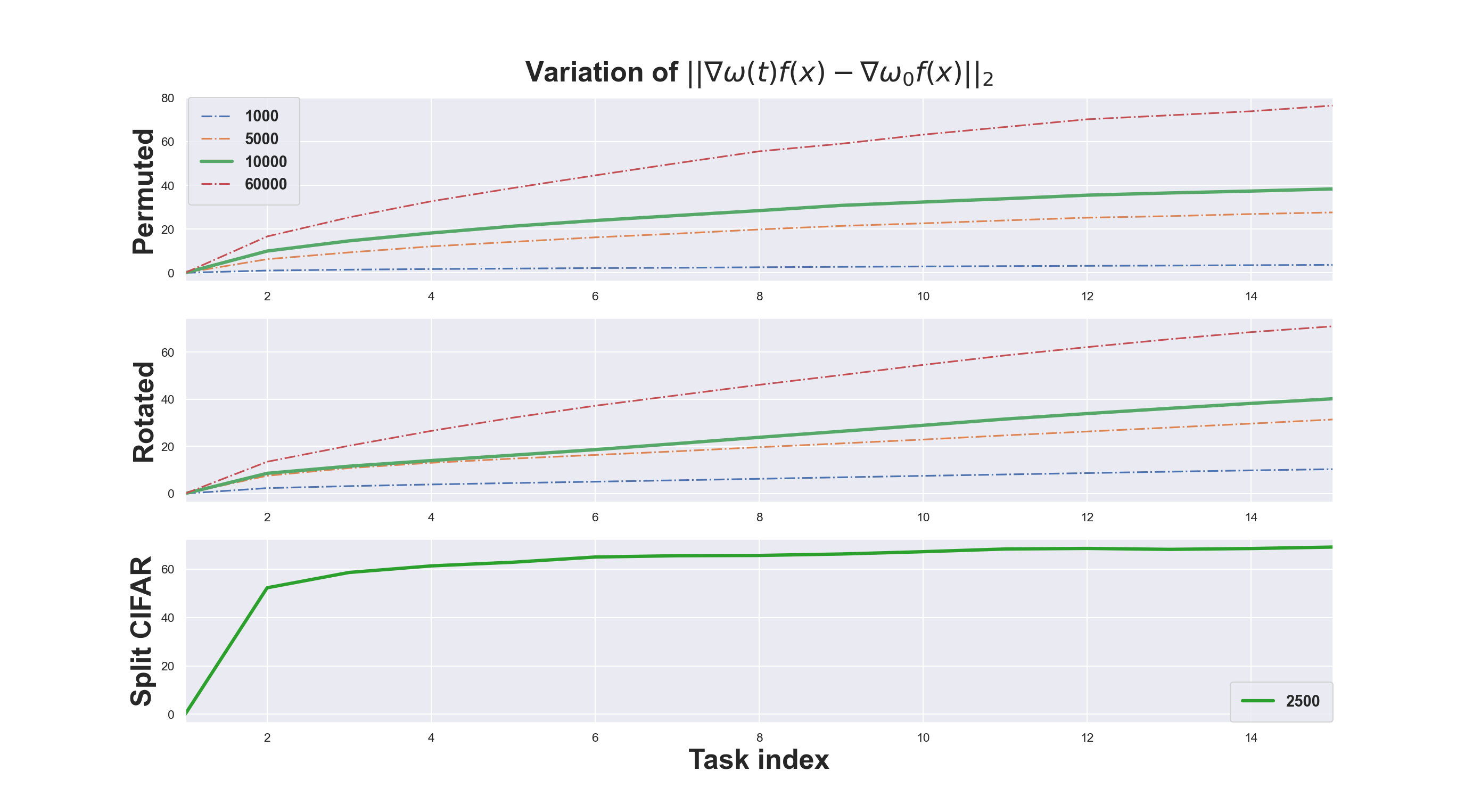
Figure 10: Variation of the NTK for different datasets size (legend).

8.11 Experimental setup and general performance

Datasets We are considering four datasets Permuted MNIST [Kirkpatrick et al., 2017], Rotated MNIST [Lopez-Paz and Ranzato, 2017], Split MNIST and Split CIFAR [Zenke et al., 2017]. For MNIST dataset, we sampled $1,000$ examples from each task leading to a total training set size of $10,000$ as in [Lopez-Paz and Ranzato, 2017, Aljundi et al., 2019a].

• Permuted MNIST is coming from the 0-9 digit dataset MNIST [LeCun et al., 1998] where each pixels have been permuted randomly. Each task corresponds to a new permutation randomly generated (but fixed along all the dataset samples).

• Rotated MNIST is the same MNIST dataset where each new task corresponds to a fixed rotation of each digit by a fixed angle. Our $15$ tasks correspond to a fixed rotation of $5$ degres with respect to the previous task.

• Split MNIST consists of $5$ binary classification tasks where we split the digit such as: $0/1$ , $2/3$ , $4/5$ , $6/7$ , $8/9$.

• Split CIFAR comes from CIFAR-100 dataset [Krizhevsky et al., 2009] which contains $100$ classes that can be grouped again into $20$ superclasses. Split CIFAR-100 [Lopez-Paz and Ranzato, 2017] is constructed by splitting the dataset into $20$ disjoincts classes sampled without replacement. The $20$ tasks are then composed of $5$ classes.

Baselines We are comparing our method PCA-OGD along with SGD, A-GEM [Chaudhry et al., 2018] and OGD [Farajtabar et al., 2020].

Optimizer We use Stochastic Gradient for each method and grid search to find hyperparameters that gave best results: learning rate of $1e-3$, batch size of $32$ and $10$ epochs for each tasks.

Performance Metrics Following [Chaudhry et al., 2018] we report the Average Accuracy $A_{T}$ and the Forgetting Measure $F_{T}$:

$$A_{T}=\frac{1}{T}\sum_{\tau=1}^{T}a_{T,\tau}$$

Where $a_{\tau,T}$ represents the accuracy of task $\tau$ at the end of the training of task $T\geq\tau$.

Forgetting Measure [Lopez-Paz and Ranzato, 2017] used the average forgetting as the performance drop of task $\tau$ over the training of later tasks:

$$F_{T}=\frac{1}{T-1}\sum_{\tau=1}^{T-1}f_{\tau}^{T}$$

where $f_{\tau}^{T}$ is defined as the highest forgetting from task $\tau$ until $T$:

$$f_{\tau}^{T}=\max_{l=\tau,...,T}a_{l,\tau}-a_{T,\tau}$$

Hyperparameters	Split MNIST	Rotated/Permuted MNIST	CIFAR-100
Dataset size (per task)	2,000	10,000	2,500
Epochs	5	10	50
Architecture	MLP	MLP	LeNet1
Hidden dimension	100	100	200
EWC regularizer	10	10	25
$\#$ tasks	5	15	20
Optimizer	SGD
Learning rate	1e-03
Batch size	32
Torch seeds	0 to 4
Memory size	100
PCA sample size $s$	3,000
samples used to compute $O^{\tau_{S}\rightarrow\tau_{T}}$ (per task)	250

Table 4: Hyperparameters used across experiments.

	Task 1	Task 2	Task 3	Task 4	Task 5	Task 6	Task 7
SGD	25.55 $\pm$ 0.99	27.79 $\pm$ 0.85	33.39 $\pm$ 1.08	40.97 $\pm$ 0.92	49.05 $\pm$ 1.07	56.05 $\pm$ 0.95	64.48 $\pm$ 0.83
EWC	49.16 $\pm$ 1.54	52.58 $\pm$ 1.85	61.0 $\pm$ 1.81	67.77 $\pm$ 1.55	72.85 $\pm$ 1.18	76.8 $\pm$ 1.1	80.05 $\pm$ 0.76
AGEM	65.48 $\pm$ 1.38	65.93 $\pm$ 1.15	72.95 $\pm$ 0.65	77.23 $\pm$ 0.55	79.38 $\pm$ 0.32	81.9 $\pm$ 0.29	84.09 $\pm$ 0.25
OGD	44.16 $\pm$ 1.52	47.06 $\pm$ 1.26	55.75 $\pm$ 0.96	63.53 $\pm$ 1.37	69.75 $\pm$ 0.36	75.67 $\pm$ 0.44	80.86 $\pm$ 0.19
PCA-OGD	52.51 $\pm$ 2.3	55.81 $\pm$ 1.79	65.21 $\pm$ 1.76	72.79 $\pm$ 1.34	79.0 $\pm$ 0.8	83.34 $\pm$ 0.57	86.65 $\pm$ 0.31

	Task 8	Task 9	Task 10	Task 11	Task 12	Task 13	Task 14	Task 15
SGD	72.75 $\pm$ 0.6	78.55 $\pm$ 0.43	84.4 $\pm$ 0.26	88.45 $\pm$ 0.27	91.08 $\pm$ 0.13	92.48 $\pm$ 0.09	93.28 $\pm$ 0.19	92.74 $\pm$ 0.15
EWC	82.71 $\pm$ 0.65	84.45 $\pm$ 0.37	86.32 $\pm$ 0.24	87.34 $\pm$ 0.31	87.47 $\pm$ 0.37	86.9 $\pm$ 0.38	85.23 $\pm$ 0.58	82.42 $\pm$ 0.65
AGEM	85.84 $\pm$ 0.12	87.47 $\pm$ 0.16	89.6 $\pm$ 0.18	91.28 $\pm$ 0.09	92.54 $\pm$ 0.18	93.13 $\pm$ 0.09	93.33 $\pm$ 0.11	92.71 $\pm$ 0.12
OGD	84.75 $\pm$ 0.41	87.39 $\pm$ 0.38	90.09 $\pm$ 0.5	91.7 $\pm$ 0.3	92.84 $\pm$ 0.28	93.03 $\pm$ 0.23	92.9 $\pm$ 0.22	91.86 $\pm$ 0.19
PCA-OGD	89.08 $\pm$ 0.1	90.62 $\pm$ 0.2	92.02 $\pm$ 0.3	92.87 $\pm$ 0.09	93.52 $\pm$ 0.17	93.18 $\pm$ 0.12	92.85 $\pm$ 0.14	91.3 $\pm$ 0.15

Table 5: Final Accuracy for Rotated MNIST (averaged over $5$ seeds $\pm 1$ std).

	Task 1	Task 2	Task 3	Task 4	Task 5	Task 6	Task 7
SGD	56.88 $\pm$ 2.85	62.18 $\pm$ 6.06	65.96 $\pm$ 2.87	66.62 $\pm$ 10.57	71.74 $\pm$ 3.0	70.86 $\pm$ 5.42	77.27 $\pm$ 1.69
EWC	77.5 $\pm$ 2.13	79.78 $\pm$ 1.63	81.91 $\pm$ 0.94	81.92 $\pm$ 0.63	81.26 $\pm$ 1.02	80.88 $\pm$ 0.89	80.91 $\pm$ 1.1
AGEM	75.34 $\pm$ 1.92	75.16 $\pm$ 1.37	79.41 $\pm$ 0.9	79.78 $\pm$ 3.22	79.87 $\pm$ 1.65	81.16 $\pm$ 1.88	82.48 $\pm$ 1.28
OGD	45.97 $\pm$ 3.6	63.25 $\pm$ 3.43	74.25 $\pm$ 2.8	78.9 $\pm$ 3.15	80.9 $\pm$ 1.42	81.99 $\pm$ 1.27	83.86 $\pm$ 0.61
PCA-OGD	35.47 $\pm$ 3.34	64.23 $\pm$ 2.05	77.98 $\pm$ 1.59	80.82 $\pm$ 1.98	83.21 $\pm$ 1.09	84.25 $\pm$ 1.39	85.89 $\pm$ 0.45

	Task 8	Task 9	Task 10	Task 11	Task 12	Task 13	Task 14	Task 15
SGD	75.14 $\pm$ 2.34	81.54 $\pm$ 2.61	83.31 $\pm$ 1.17	85.27 $\pm$ 1.71	86.48 $\pm$ 0.49	88.34 $\pm$ 0.29	89.73 $\pm$ 0.48	90.85 $\pm$ 0.16
EWC	80.98 $\pm$ 0.94	80.4 $\pm$ 1.33	80.2 $\pm$ 1.18	79.77 $\pm$ 1.27	78.6 $\pm$ 0.91	77.92 $\pm$ 0.8	77.3 $\pm$ 0.58	76.28 $\pm$ 0.67
AGEM	82.81 $\pm$ 1.09	85.86 $\pm$ 0.67	85.56 $\pm$ 0.85	86.44 $\pm$ 1.22	87.65 $\pm$ 0.81	88.81 $\pm$ 0.34	89.91 $\pm$ 0.25	90.79 $\pm$ 0.21
OGD	85.42 $\pm$ 0.59	86.69 $\pm$ 0.5	86.84 $\pm$ 0.62	87.86 $\pm$ 0.65	88.68 $\pm$ 0.36	89.28 $\pm$ 0.31	89.88 $\pm$ 0.23	90.45 $\pm$ 0.16
PCA-OGD	87.08 $\pm$ 0.26	87.46 $\pm$ 0.77	87.9 $\pm$ 0.5	88.34 $\pm$ 0.44	89.16 $\pm$ 0.39	89.65 $\pm$ 0.14	89.93 $\pm$ 0.17	90.29 $\pm$ 0.2

Table 6: Final Accuracy for Permuted MNIST (averaged over $5$ seeds $\pm 1$ std).

	Task 1	Task 2	Task 3	Task 4	Task 5	Task 6	Task 7	Task 8	Task 9	Task 10
SGD	48.92 $\pm$ 5.11	40.96 $\pm$ 2.7	46.52 $\pm$ 6.45	40.2 $\pm$ 7.27	56.36 $\pm$ 8.12	44.76 $\pm$ 6.08	54.32 $\pm$ 4.9	44.52 $\pm$ 5.41	46.24 $\pm$ 6.29	59.88 $\pm$ 7.56
EWC	63.28 $\pm$ 2.44	62.32 $\pm$ 7.5	57.36 $\pm$ 5.88	56.0 $\pm$ 6.39	73.56 $\pm$ 6.42	52.32 $\pm$ 5.96	64.92 $\pm$ 3.03	62.44 $\pm$ 2.89	53.04 $\pm$ 6.24	70.48 $\pm$ 5.09
AGEM	38.88 $\pm$ 2.81	37.0 $\pm$ 5.34	37.28 $\pm$ 5.62	32.44 $\pm$ 8.53	42.4 $\pm$ 12.14	36.72 $\pm$ 4.66	41.12 $\pm$ 5.16	39.36 $\pm$ 4.22	41.92 $\pm$ 6.3	47.08 $\pm$ 8.52
OGD	52.04 $\pm$ 2.92	57.84 $\pm$ 5.83	59.96 $\pm$ 3.77	56.32 $\pm$ 1.47	74.12 $\pm$ 2.25	58.04 $\pm$ 2.75	69.24 $\pm$ 1.18	66.36 $\pm$ 3.66	60.84 $\pm$ 2.17	77.84 $\pm$ 2.2
PCA-OGD	57.24 $\pm$ 2.55	63.08 $\pm$ 4.96	66.16 $\pm$ 0.83	61.52 $\pm$ 1.09	75.32 $\pm$ 6.88	62.88 $\pm$ 1.45	73.28 $\pm$ 1.06	70.48 $\pm$ 1.67	66.32 $\pm$ 1.14	80.28 $\pm$ 1.22

	Task 11	Task 12	Task 13	Task 14	Task 15	Task 16	Task 17	Task 18	Task 19	Task 20
SGD	67.56 $\pm$ 4.21	49.64 $\pm$ 8.46	66.4 $\pm$ 4.6	58.68 $\pm$ 4.78	65.68 $\pm$ 5.11	54.8 $\pm$ 13.41	63.6 $\pm$ 3.84	57.84 $\pm$ 4.5	75.16 $\pm$ 2.54	80.12 $\pm$ 2.41
EWC	77.92 $\pm$ 2.36	67.4 $\pm$ 1.51	74.44 $\pm$ 1.83	68.28 $\pm$ 3.08	72.64 $\pm$ 1.87	67.88 $\pm$ 3.73	67.08 $\pm$ 3.67	53.08 $\pm$ 5.02	73.32 $\pm$ 1.18	71.32 $\pm$ 6.05
AGEM	54.68 $\pm$ 7.95	39.48 $\pm$ 11.16	52.52 $\pm$ 12.46	50.36 $\pm$ 7.41	55.4 $\pm$ 12.14	55.16 $\pm$ 1.8	54.92 $\pm$ 9.64	50.28 $\pm$ 10.96	65.56 $\pm$ 5.36	78.52 $\pm$ 1.01
OGD	80.44 $\pm$ 1.93	67.8 $\pm$ 2.99	80.4 $\pm$ 1.04	74.56 $\pm$ 0.8	77.92 $\pm$ 1.93	72.36 $\pm$ 0.82	75.0 $\pm$ 0.83	73.0 $\pm$ 1.48	79.52 $\pm$ 1.39	81.88 $\pm$ 1.73
PCA-OGD	82.56 $\pm$ 0.74	71.84 $\pm$ 1.81	81.88 $\pm$ 1.52	76.08 $\pm$ 1.51	80.4 $\pm$ 0.95	73.52 $\pm$ 1.39	76.52 $\pm$ 0.53	73.0 $\pm$ 1.63	80.36 $\pm$ 1.82	81.28 $\pm$ 0.72

Table 7: Final Accuracy for Split CIFAR (averaged over $5$ seeds $\pm 1$ std).

	Task 1	Task 2	Task 3	Task 4	Task 5
SGD	99.35 $\pm$ 0.2	88.62 $\pm$ 5.21	94.85 $\pm$ 1.69	98.1 $\pm$ 0.38	94.6 $\pm$ 0.4
EWC	99.34 $\pm$ 0.19	88.36 $\pm$ 5.38	94.96 $\pm$ 1.37	98.09 $\pm$ 0.39	94.56 $\pm$ 0.49
AGEM	99.5 $\pm$ 0.22	85.92 $\pm$ 7.36	93.31 $\pm$ 2.13	98.07 $\pm$ 0.42	94.44 $\pm$ 0.82
OGD	99.64 $\pm$ 0.09	92.24 $\pm$ 1.49	95.75 $\pm$ 0.4	98.22 $\pm$ 0.39	94.41 $\pm$ 0.4
PCA-OGD	99.67 $\pm$ 0.08	92.22 $\pm$ 1.67	95.37 $\pm$ 0.72	98.39 $\pm$ 0.28	94.14 $\pm$ 0.42

Table 8: Final Accuracy for Split MNIST (averaged over $5$ seeds $\pm 1$ std).

8.12 Worst-case scenario for PCA-OGD: data spread uniformly along all directions

In this section, we present a toy example which highlights the drawbacks of PCA-OGD against Catastrophic Forgetting in comparison with OGD, in the special case where magnitude of eigenvalues are spread out.

Experiments

In this section, we build a worst case scneario where datapoints $\{X^{\tau}\}_{\tau=1}^{T}$ are spread uniformly across all directions. We consider a regression task with a linear model $f_{\tau}(X^{\tau})=(X^{\tau})^{\top}({\omega_{\tau}(t)-\omega_{\tau-1}^{\star}})$ where $X^{\tau}\in\mathbb{R}^{n_{\tau}\times p}$, $\omega\in\mathbb{R}^{p}$, $\tau\in[T]$. We generate the data as follows for all $\tau\in[T]$:

$$X^{\tau}\sim\mathcal{N}(\mu_{x_{\tau},\sigma_{x_{\tau}}})$$

$$\omega_{\tau}^{\star}\sim\mathcal{N}(\mu_{\omega_{\tau}},\sigma_{\omega_{\tau}})$$

$$y_{\tau}=(X^{\tau})^{\top}\omega_{\tau}^{\star}+\epsilon_{\tau}$$

$$\epsilon_{\tau}\sim\mathcal{N}(0,\sigma_{\epsilon_{\tau}})$$

We are considering Mean Square Error (MSE) for the loss function: $\mathcal{L}_{\tau}=\frac{1}{n_{\tau}}\displaystyle{\sum_{i=1}^{n_{\tau}}}(y^{\tau}_{i}-f_{\tau}(x^{\tau}_{i}))^{2},\hskip 10.00002pt\forall\tau\in[T]$.

Note in this setting, the kernel is simply the which is simply the gradient kernel matrix of the dataset :

$$\phi(X^{\tau})\phi(X^{\tau})^{\top}=\nabla_{\omega}f_{\tau}(X^{\tau})\nabla_{\omega}f_{\tau}(X^{\tau})^{\top}=X^{\tau}(X^{\tau})^{\top}\in\mathbb{R}^{n_{\tau}\times n_{\tau}}$$

As shown below in Figure 11(a) the eigenvalues of the PCA decomposition of $X^{\tau}(X^{\tau})^{\top}$ are of the same magnitude order and taking the first $25$ components only represents $26\%$ of the explained variance. We trained the model on $15$ tasks with a total memory of $25$ per tasks. We only show below the testing error and forgetting error of the first $9$ tasks. As expected, PCA-OGD incurs drastic variation of its loss function while OGD shows practically no forgetting.

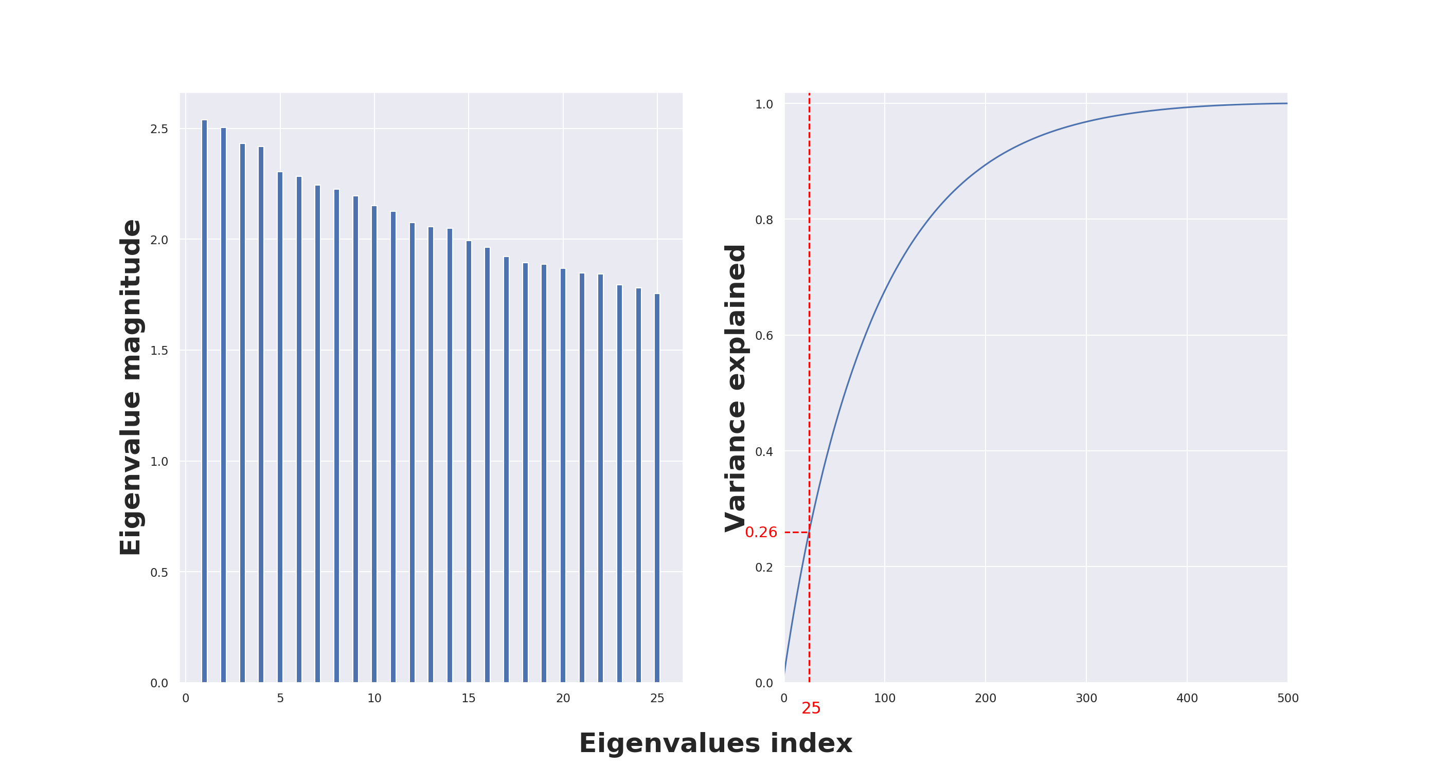
(a)

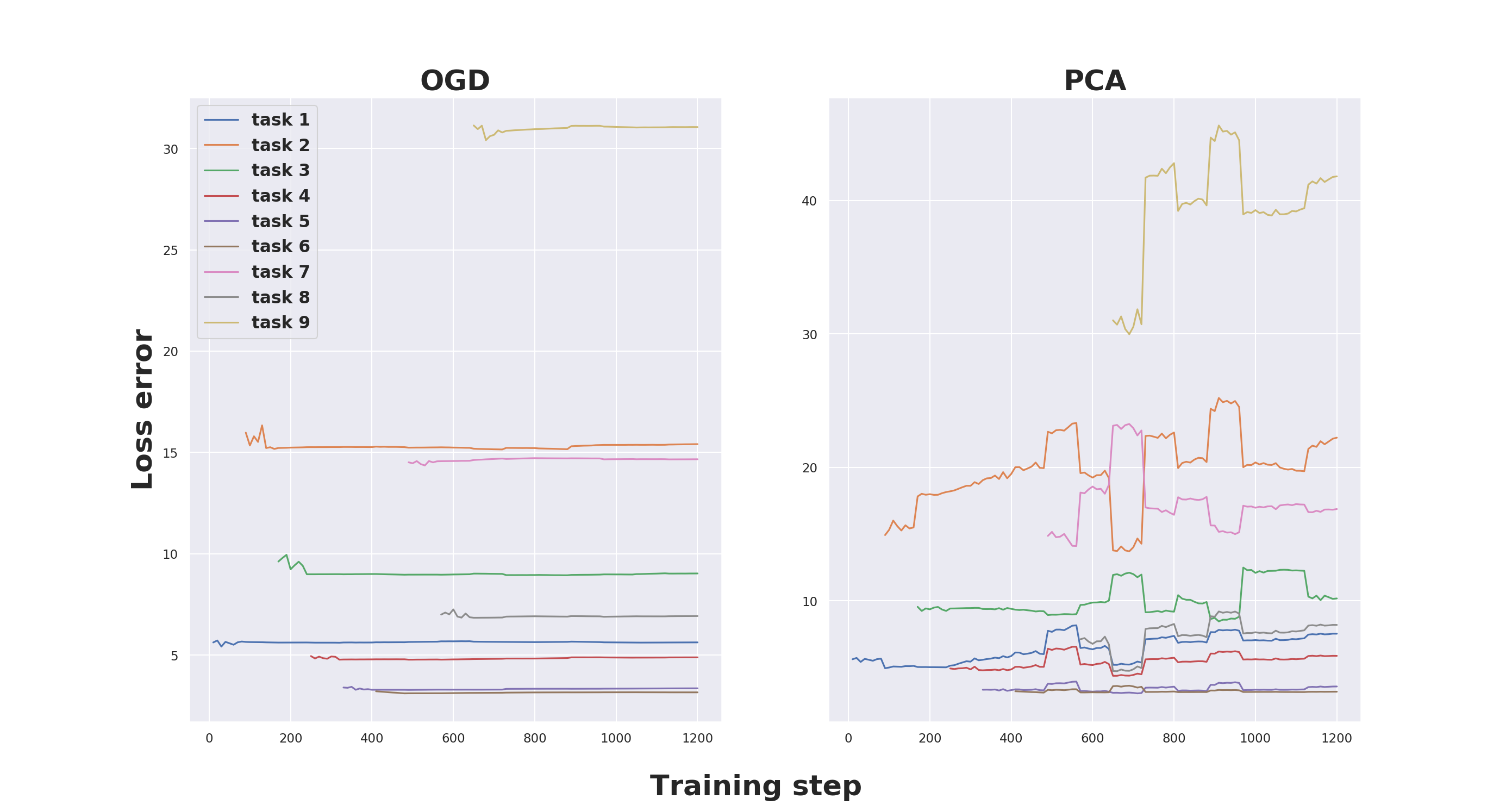
(b)

8.13 Pseudo-code for GEM-NT

Input : A task sequence $\mbox{$\mathcal{T}$}_{1},\mbox{$\mathcal{T}$}_{2},\ldots$, learning rate $\eta$, components to keep $d$

1. Initialize $S_{1}\leftarrow\{\}$ ; $\omega\leftarrow\omega_{0}$

2. for Task ID $\tau=1,2,3,\ldots$ do

       repeat

             $\mbox{$\mbox{$\mathbf{g}$}$}\leftarrow$ Stochastic Batch Gradient for $\mbox{$\mathcal{T}$}_{\tau}$ at $\omega$;

             // Orthogonal updates $\tilde{\mbox{$\mbox{$\mathbf{g}$}$}}=\mbox{$\mbox{$\mathbf{g}$}$}-\sum_{(x_{k},y_{k})\in\mbox{$\mathcal{S}$}_{k},{\color[rgb]{1,0,0}k=1,..,\tau-1}}\nabla\mathcal{L}^{\tau}_{\lambda}(x_{k};y_{k}))$;

             $\omega\leftarrow\omega-\eta\tilde{\mbox{$\mbox{$\mathbf{g}$}$}}$

      until convergence;

      // Compute loss gradient Sample $d$ elements $(x_{\tau},y_{\tau})$ from $\mbox{$\mathcal{T}$}_{\tau}$   $S_{\tau}\leftarrow\{(x_{\tau},y_{\tau})\}$  

end for

Algorithm 2 GEM-NT for Continual Learning

8.14 Computational overhead of PCA-OGD

The only additional step of PCA-OGD over OGD is the PCA operation. The complexity of the Graham Schmidt (GS) step is $O(M^{2}p)$ where $M$ is the memory size and $p$ the number of parameters. The PCA operation has complexity $O(n^{2}p)$ where $n\ll p$ are the first $n$ components to keep. However, $n=M/T$ with $T$ being the number of tasks hence there is no computational overhead for the PCA step: PCA-OGD and OGD have the same asymptotic complexity.

8.15 Eigenvalues evolution of the NTK overlap matrix between the source and target task

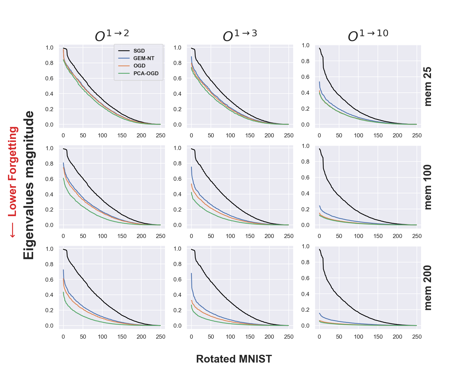
Figure 12: Eigenvalues of the overlap matrix $O^{\tau_{S}\rightarrow\tau_{T}}$ for different memozy size and methods. Increasing memory gives better advantage to PCA-OGD.

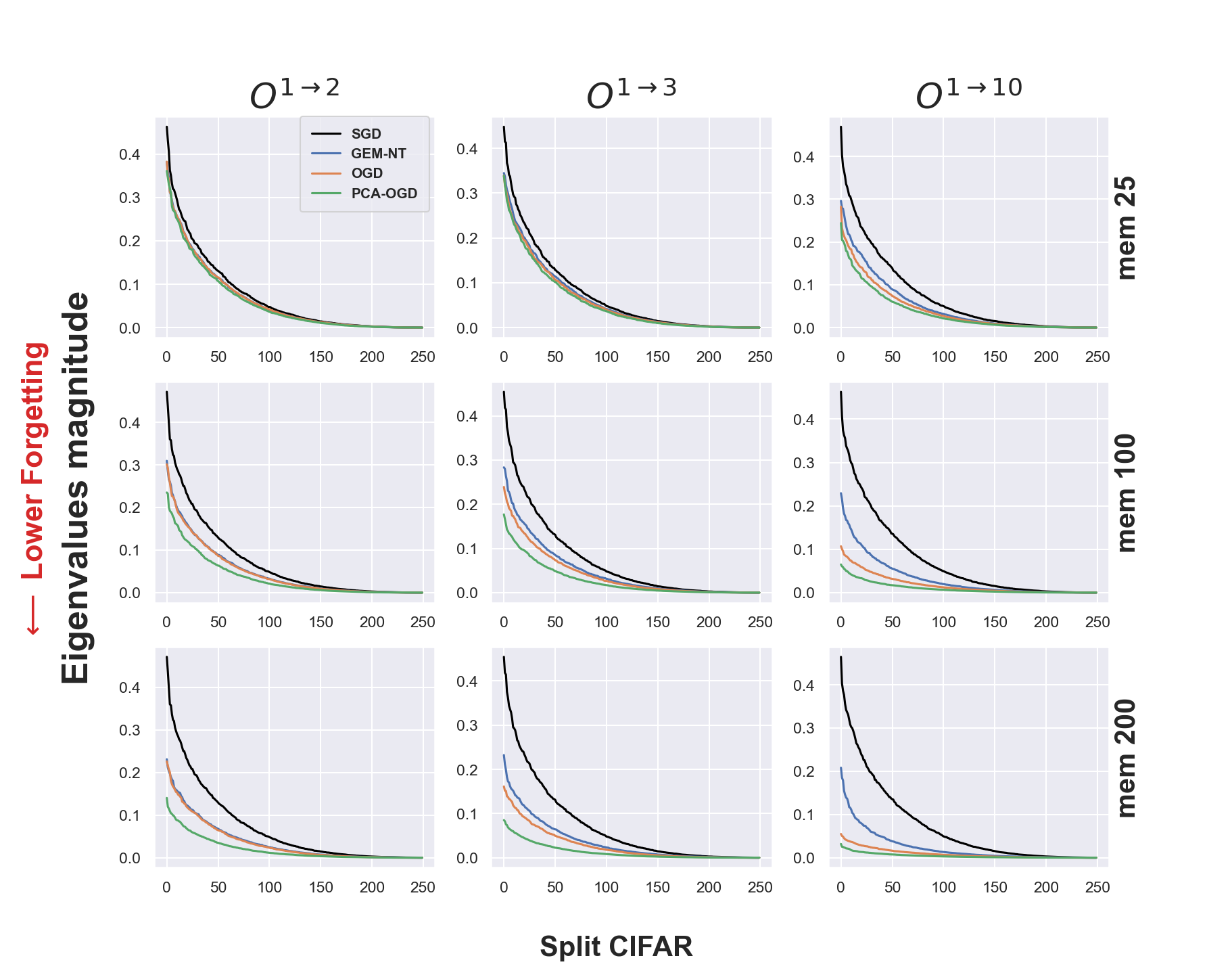
Figure 13: Eigenvalues of the overlap matrix $O^{\tau_{S}\rightarrow\tau_{T}}$ for different memozy size and methods. Increasing memory gives better advantage to PCA-OGD.

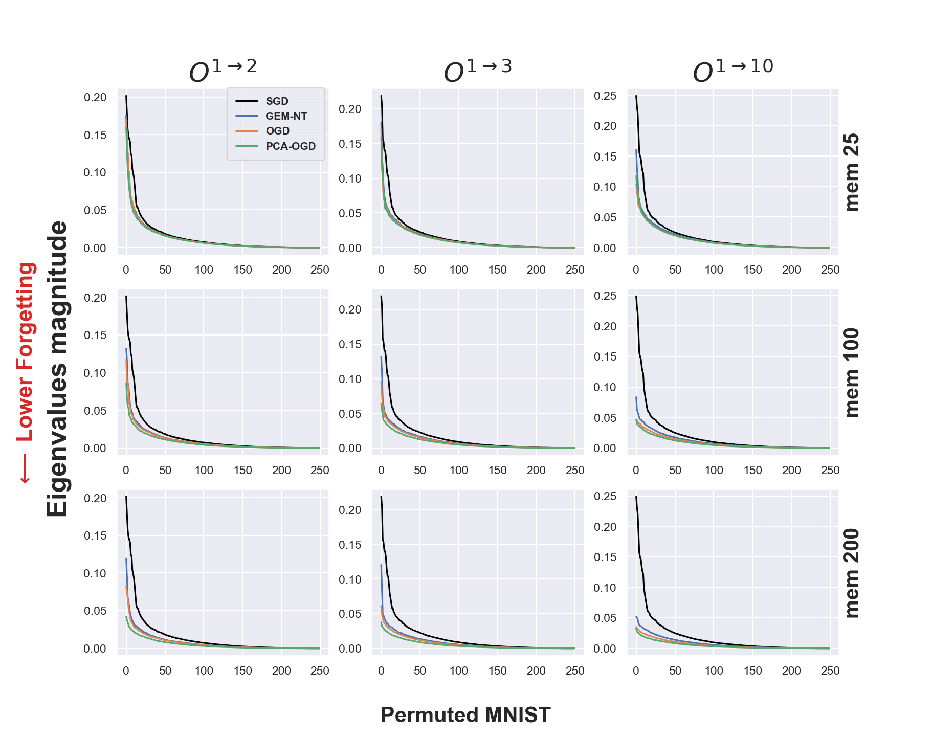
Figure 14: Eigenvalues of the overlap matrix $O^{\tau_{S}\rightarrow\tau_{T}}$ for different memozy size and methods. Since there is no Pattern accross task of Permuted MNIST, PCA-OGD does not take advantage of keeping principal eigenvalues directions.

References

- Aljundi et al. [2019a] Rahaf Aljundi, Eugene Belilovsky, Tinne Tuytelaars, Laurent Charlin, Massimo Caccia, Min Lin, and Lucas Page-Caccia. Online continual learning with maximal interfered retrieval. In Advances in Neural Information Processing Systems, pages 11849–11860, 2019a.
- Aljundi et al. [2019b] Rahaf Aljundi, Min Lin, Baptiste Goujaud, and Yoshua Bengio. Gradient based sample selection for online continual learning. In Advances in Neural Information Processing Systems, pages 11816–11825, 2019b.
- Arora et al. [2019] Sanjeev Arora, Simon S Du, Wei Hu, Zhiyuan Li, Russ R Salakhutdinov, and Ruosong Wang. On exact computation with an infinitely wide neural net. In Advances in Neural Information Processing Systems, pages 8141–8150, 2019.
- Bennani et al. [2020] Mehdi Abbana Bennani, Thang Doan, and Masashi Sugiyama. Generalisation guarantees for continual learning with orthogonal gradient descent, 2020.
- Chaudhry et al. [2018] Arslan Chaudhry, Marc’Aurelio Ranzato, Marcus Rohrbach, and Mohamed Elhoseiny. Efficient lifelong learning with a-gem. arXiv preprint arXiv:1812.00420, 2018.
- Chen and Liu [2018] Zhiyuan Chen and Bing Liu. Lifelong machine learning. Synthesis Lectures on Artificial Intelligence and Machine Learning, 12(3):1–207, 2018.
- De Lange et al. [2019] Matthias De Lange, Rahaf Aljundi, Marc Masana, Sarah Parisot, Xu Jia, Ales Leonardis, Gregory Slabaugh, and Tinne Tuytelaars. Continual learning: A comparative study on how to defy forgetting in classification tasks. arXiv preprint arXiv:1909.08383, 2019.
- Du et al. [2018] Simon S Du, Xiyu Zhai, Barnabas Poczos, and Aarti Singh. Gradient descent provably optimizes over-parameterized neural networks. arXiv preprint arXiv:1810.02054, 2018.
- Farajtabar et al. [2020] Mehrdad Farajtabar, Navid Azizan, Alex Mott, and Ang Li. Orthogonal gradient descent for continual learning. In International Conference on Artificial Intelligence and Statistics, pages 3762–3773, 2020.
- Farquhar and Gal [2018] Sebastian Farquhar and Yarin Gal. Towards robust evaluations of continual learning. arXiv preprint arXiv:1805.09733, 2018.
- Goodfellow et al. [2013] Ian J Goodfellow, Mehdi Mirza, Da Xiao, Aaron Courville, and Yoshua Bengio. An empirical investigation of catastrophic forgetting in gradient-based neural networks. arXiv preprint arXiv:1312.6211, 2013.
- Jacot et al. [2018] Arthur Jacot, Franck Gabriel, and Clément Hongler. Neural tangent kernel: Convergence and generalization in neural networks. In Advances in neural information processing systems, pages 8571–8580, 2018.
- Kemker et al. [2017] Ronald Kemker, Marc McClure, Angelina Abitino, Tyler Hayes, and Christopher Kanan. Measuring catastrophic forgetting in neural networks. arXiv preprint arXiv:1708.02072, 2017.
- Kirkpatrick et al. [2017] James Kirkpatrick, Razvan Pascanu, Neil Rabinowitz, Joel Veness, Guillaume Desjardins, Andrei A Rusu, Kieran Milan, John Quan, Tiago Ramalho, Agnieszka Grabska-Barwinska, et al. Overcoming catastrophic forgetting in neural networks. Proceedings of the national academy of sciences, 114(13):3521–3526, 2017.
- Krizhevsky et al. [2009] Alex Krizhevsky et al. Learning multiple layers of features from tiny images. 2009.
- LeCun et al. [1998] Yann LeCun, Léon Bottou, Yoshua Bengio, and Patrick Haffner. Gradient-based learning applied to document recognition. Proceedings of the IEEE, 86(11):2278–2324, 1998.
- Lee et al. [2019] Jaehoon Lee, Lechao Xiao, Samuel S Schoenholz, Yasaman Bahri, Roman Novak, Jascha Sohl-Dickstein, and Jeffrey Pennington. Wide neural networks of any depth evolve as linear models under gradient descent. arXiv preprint arXiv:1902.06720, 2019.
- Lopez-Paz and Ranzato [2017] David Lopez-Paz and Marc’Aurelio Ranzato. Gradient episodic memory for continual learning. In Advances in neural information processing systems, pages 6467–6476, 2017.
- Mallya and Lazebnik [2018] Arun Mallya and Svetlana Lazebnik. Packnet: Adding multiple tasks to a single network by iterative pruning. In Proceedings of the IEEE Conference on Computer Vision and Pattern Recognition, pages 7765–7773, 2018.
- McCloskey and Cohen [1989] Michael McCloskey and Neal J Cohen. Catastrophic interference in connectionist networks: The sequential learning problem. In Psychology of learning and motivation, volume 24, pages 109–165. Elsevier, 1989.
- Mirzadeh et al. [2020] Seyed Iman Mirzadeh, Mehrdad Farajtabar, Razvan Pascanu, and Hassan Ghasemzadeh. Understanding the role of training regimes in continual learning. arXiv preprint arXiv:2006.06958, 2020.
- Nguyen et al. [2019] Cuong V Nguyen, Alessandro Achille, Michael Lam, Tal Hassner, Vijay Mahadevan, and Stefano Soatto. Toward understanding catastrophic forgetting in continual learning. arXiv preprint arXiv:1908.01091, 2019.
- Nguyen et al. [2020] Giang Nguyen, Shuan Chen, Tae Joon Jun, and Daeyoung Kim. Explaining how deep neural networks forget by deep visualization, 2020.
- Pan et al. [2020] Pingbo Pan, Siddharth Swaroop, Alexander Immer, Runa Eschenhagen, Richard E Turner, and Mohammad Emtiyaz Khan. Continual deep learning by functional regularisation of memorable past. arXiv preprint arXiv:2004.14070, 2020.
- Parisi et al. [2019] German I Parisi, Ronald Kemker, Jose L Part, Christopher Kanan, and Stefan Wermter. Continual lifelong learning with neural networks: A review. Neural Networks, 113:54–71, 2019.
- Ramasesh et al. [2020] Vinay V Ramasesh, Ethan Dyer, and Maithra Raghu. Anatomy of catastrophic forgetting: Hidden representations and task semantics. arXiv preprint arXiv:2007.07400, 2020.
- Rosenfeld and Tsotsos [2018] Amir Rosenfeld and John K Tsotsos. Incremental learning through deep adaptation. IEEE transactions on pattern analysis and machine intelligence, 2018.
- Silver [2011] Daniel L Silver. Machine lifelong learning: challenges and benefits for artificial general intelligence. In International conference on artificial general intelligence, pages 370–375. Springer, 2011.
- Thrun [1995] Sebastian Thrun. A lifelong learning perspective for mobile robot control. In Intelligent robots and systems, pages 201–214. Elsevier, 1995.
- Toneva et al. [2018] Mariya Toneva, Alessandro Sordoni, Remi Tachet des Combes, Adam Trischler, Yoshua Bengio, and Geoffrey J Gordon. An empirical study of example forgetting during deep neural network learning. arXiv preprint arXiv:1812.05159, 2018.
- Wedin [1983] Per Åke Wedin. On angles between subspaces of a finite dimensional inner product space. In Matrix Pencils, pages 263–285. Springer, 1983.
- Xie et al. [2020] Zeke Xie, Fengxiang He, Shaopeng Fu, Issei Sato, Dacheng Tao, and Masashi Sugiyama. Artificial neural variability for deep learning: On overfitting, noise memorization, and catastrophic forgetting. arXiv preprint arXiv:2011.06220, 2020.
- Yin et al. [2020] Dong Yin, Mehrdad Farajtabar, and Ang Li. Sola: Continual learning with second-order loss approximation. arXiv preprint arXiv:2006.10974, 2020.
- Yu et al. [2020] Tianhe Yu, Saurabh Kumar, Abhishek Gupta, Sergey Levine, Karol Hausman, and Chelsea Finn. Gradient surgery for multi-task learning. Advances in Neural Information Processing Systems, 33, 2020.
- Zenke et al. [2017] Friedemann Zenke, Ben Poole, and Surya Ganguli. Continual learning through synaptic intelligence. Proceedings of machine learning research, 70:3987, 2017.
- Zhu and Knyazev [2013] Peizhen Zhu and Andrew V Knyazev. Angles between subspaces and their tangents. Journal of Numerical Mathematics, 21(4):325–340, 2013.