Neural-network analysis of Parton Distribution Functions from Ioffe-time pseudodistributions

Abstract

We extract two nonsinglet nucleon Parton Distribution Functions from lattice QCD data for reduced Ioffe-time pseudodistributions. We perform such analysis within the NNPDF framework, considering data coming from different lattice ensembles and discussing in detail the treatment of the different source of systematics involved in the fit. We introduce a recipe for taking care of systematics and use it to perform our extraction of light-cone PDFs.

1 Introduction

Parton Distribution Functions (PDFs), encoding the structure of the proton in terms of quarks and gluons, are one of the main ingredients required to do precise high-energy phenomenology. The available PDFs sets are extracted through global fits over experimental data Ball:2017nwa ; Dulat:2015mca ; Alekhin:2017kpj ; Martin:2009iq ; Buckley:2014ana . Their non-perturbative nature makes them a natural candidate for a lattice QCD investigation, however it has been known for a long time that it is not possible to obtain them directly from first principle computations, due to the Euclidean metric of the lattice. In the last few years, several methods have been formulated Lin:2020rut ; Constantinou:2020pek , which would allow us to compute on the lattice specific quantities that, in turn, can be related to PDFs through a factorization theorem. For a detailed discussion of the theoretical background, we refer the reader to recent reviews such as Refs. Radyushkin:2019mye ; Cichy:2018mum ; Monahan:2018euv ; Ji:2020ect .

Examples of such quantities are the equal time correlators underlying the definition of quasi- and pseudo-PDFs PhysRevLett.110.262002 ; Radyushkin:2017cyf , given by

$$M^{(0)}_{\mu}\left(z,P\right) =\langle P|\bar{\psi}^{(0)}\left(z\right)\gamma_{\mu}\,U^{(0)}\left(z,0\right)\psi^{(0)}\left(0\right)|P\rangle\,,$$ (1.1)

with $P$ denoting the momentum of the external proton states, while the suffix $(0)$ reminds us that these are bare quantities. The matrix element of the vector bilocal operator of Eq. (1.1) can be decomposed in terms of two form factors which only depend on the Lorentz invariants $z^{2}$ and $\nu\equiv-z\cdot P$ as

$$M^{(0)}_{\mu}\left(z,P\right)=2P_{\mu}\,\mathcal{M}^{(0)}\left(\nu,z^{2}\right)+z_{\mu}\,\mathcal{N}^{(0)}\left(\nu,z^{2}\right)\,.$$ (1.2)

As pointed out in Musch:2010ka , only the first form factor, $\mathcal{M}^{(0)}$, contains leading twist information. This can be seen by choosing a light-cone separation $z=\left(0,z^{-},0_{\perp}\right)$ together with $\gamma^{\mu}=\gamma^{+}$ and $P=\left(P^{+},0,0_{\perp}\right)$, then we get

$$M^{(0)}_{+}\left(z,P\right)=2P_{+}\,\mathcal{M}^{(0)}\left(\nu,0\right)=2P_{+}\,\int_{-1}^{1}dx\,e^{ix\nu}f^{(0)}\left(x\right)$$ (1.3)

with $f^{(0)}\left(x\right)$ being the bare collinear nonsinglet parton distribution. Because of the light-cone separation $z$ involved in its definition, $M^{(0)}_{+}$ is not directly computable on a Euclidean lattice. We can define a different quantity that is amenable to lattice simulations by choosing a purely spatial separation, $z=\left(0,0,0,z_{3}\right)$, together with $\gamma^{\mu}=\gamma^{0}$ and $P=\left(E,0,0,P_{3}\right)$. Then taking the time component of Eq. (1.2) we get

$$M^{(0)}_{0}\left(z,P\right)=2E\,\mathcal{M}^{(0)}\left(\nu,-z_{3}^{2}\right)\,.$$ (1.4)

The correlators defined in Eqs. (1.3) and (1.4) are known in the literature as (bare) Ioffe-time distribution (ITD) and pseudodistribution (pseudo-ITD) respectively Radyushkin:2017cyf ; Braun:1994jq . For $z_{3}^{2}\neq 0$, in addition to usual ultraviolet (UV) divergences (leading to coupling renormalization), they have specific link-related UV divergences, which are regularized by a finite lattice spacing $a$. Thus, $\mathcal{M}^{(0)}\left(\nu,-z_{3}^{2}\right)$ is in fact $\mathcal{M}^{(0)}\left(\nu,-z_{3}^{2};a^{2}\right)$.

The $a\to 0$ UV divergences are multiplicatively renormalizable Ji:2017oey ; Ishikawa:2017faj . The relevant renormalization factor $Z(z_{3}^{2},a^{2})$ does not depend on $\nu$ and, for small $z_{3}^{2}$, is known at one loop. Its explicit form is inessential if one introduces the so-called reduced Ioffe-time pseudo-distributions first defined in Ref. Radyushkin:2017cyf as

$$\mathfrak{M}\left(\nu,z_{3}^{2}\right)=\frac{\mathcal{M}\left(\nu,-z_{3}^{2};a^{2}\right)}{\mathcal{M}\left(0,-z_{3}^{2};a^{2}\right)}.$$ (1.5)

The $Z$-factors of the numerator and denominator are the same and cancel in the ratio leaving the reduced distribution on the left-hand side without any residual dependence on the lattice spacing.

Working in the small-$z_{3}^{2}$ limit, the pseudo-ITD can be matched at one-loop level to the corresponding ITD through a finite perturbative kernel, expressing the pseudo-ITD in terms of the collinear PDFs through a factorization formula based on the operator product expansion (OPE). The computation of the relevant QCD diagrams has been performed in a number of independent papers. The original QCD computation is reported, for example, in Refs. Radyushkin:2017lvu ; Radyushkin:2016hsy ; Izubuchi:2018srq ; Ji:2017rah . A simple discussion of the basic features of the derivation of the factorization formula in non-gauge theories can be found in Ref. DelDebbio:2020cbz .

The QCD result reads

$$\mathfrak{M}\left(\nu,z_{3}^{2}\right)=\int_{-1}^{1}dx\,C\left(x\nu,\mu^{2}z_{3}^{2}\right)f\left(x,\mu^{2}\right)+\mathcal{O}\left(z_{3}^{2}\Lambda^{2}\right)\,,$$ (1.6)

with

$$C\left(\xi,\mu^{2}z_{3}^{2}\right)=e^{i\xi}-\frac{\alpha_{s}}{2\pi} C_{F}\int_{0}^{1}dw\,\biggl{[}\frac{1+w^{2}}{1-w}\log\left(z_{3}^{2}\mu^{2}\frac{e^{2\gamma_{E}+1}}{4}\right)$$

$$+4\frac{\log\left(1-w\right)}{1-w}-2\left(1-w\right)\biggr{]}_{+}e^{i\xi w}+\mathcal{O}\left(\alpha_{s}^{2}\right).$$ (1.7)

Eqs. (1.6),  (1) allow to relate collinear PDFs to quantities which are computable in lattice QCD simulations, through a factorized expression similar to those relating collinear PDFs to physical cross sections. In the spirit of the “good lattice cross sections” proposed in Refs. Ma:2017pxb ; Ma:2014jla , this formula can be used in a fitting framework, to extract PDFs from lattice data, performing the same kind of analysis which is usually done when considering experimental data. This approach was first studied in Ref. Karpie2019 , and subsequently in Ref. Izubuchi:2019lyk ; Cichy2019 ; Gao:2020ito . In Ref. Cichy2019 , it has been implemented within the NNPDF fitting environment. Considering data for quasi-PDFs matrix elements produced in Refs. Alexandrou:2018pbm ; Alexandrou:2019lfo and starting from the momentum space factorization formula connecting quasi-PDFs to collinear PDFs, upon numerical implementation of the Fourier transform an expression analogous to Eq. (1.6) was obtained, relating parton distributions directly to position space quasi-PDFs matrix elements. A similar analysis was very recently performed by the JAM collaboration in Ref. Bringewatt:2020ixn for the spin-averaged and spin-dependent PDFs employing quasi-PDF lattice data.

In the present work we perform an analogous exercise considering this time the reduced pseudo-ITD approach, implementing within the NNPDF environment the lattice data presented in Ref. Joo:2019jct ; Joo:2020spy , and using the position space factorization formula of Eqs. (1.6), (1). This, besides being a complementary exercise to the one performed in Ref. Cichy2019 , has also some practical advantages. First, when working in the pseudo-ITD approach, the factorization is realized in the limit of small-$z^{2}$. Unlike in the quasi-PDFs approach, where the factorization is realized for high values of $P$, here we are allowed to keep in the analysis data coming from a wide range of momentum values, without having to remove those with lower $P$. This advantage is particularly important, because in lattice QCD, the low momentum data are significantly more precise for a fixed computational cost. Second, we can directly use the position space factorization formula of Eq. (1.6), relying on the analytical expression for the perturbative coefficient of Eq. (1) and without having to perform the numerical Fourier transform described in the appendix A of Ref. Cichy2019 .

In this article we extend the general strategy that has been developed within the NNPDF framework and which allows us to systematically extract parton distributions from the available lattice data. In the implementation of this idea once the lattice data have reached some level of maturity in terms of precision and systematic effects, one could combine data from all pertinent lattice formalisms such as quasi-distributions  Lin:2014zya ; Chen:2016utp ; Alexandrou:2015rja ; Alexandrou:2016jqi ; Monahan:2016bvm ; Zhang:2017bzy ; Alexandrou:2017huk ; Green:2017xeu ; Alexandrou:2018pbm ; Chen:2018xof ; Alexandrou:2018eet ; Lin:2018qky ; Fan:2018dxu ; Liu:2018hxv ; Alexandrou:2019lfo ; Izubuchi:2019lyk ; Green:2020xco ; Chai:2020nxw ; Lin:2020ssv ; Alexandrou:2020zbe and pseudo-distributions  Orginos:2017kos ; Karpie:2018zaz ; Joo:2019jct ; Joo:2019bzr ; Joo:2020spy ; Bhat:2020ktg ; Fan:2020cpa ; Gao:2020ito . One can also include results from the so-called “Good Lattice Cross-Sections” (LCS) approach, which is described in Ma:2017pxb and represents a general framework, where one computes matrix elements that can be factorized into PDFs at short distances. Papers Bali:2017gfr ; Bali:2018spj ; Sufian:2019bol ; Bali:2019ecy ; Sufian:2020vzb describe implementations of the latter formalism. Clearly a global analysis only makes sense after having scrutinised each set of data individually, and having understood the systematics that affect them. The structure of the paper is as follows. In Sec. 2 we define the lattice observable considered in the fit, describe the corresponding data and briefly recall the main features of the NLO terms entering the factorization formulas. In Sec. 3 we present the first set of results: we consider the fits where only the statistical uncertainties of the lattice data are taken into account. Analyzing data from different lattice ensembles we show that, in general, without accounting for systematic effects it is not possible to obtain a good fit. In Sec. 4 we discuss and quantify some of the systematic uncertainties affecting the lattice data. We include them into the analysis and study their impact on the final PDFs and on the fit quality. Sec. 5 summarizes our conclusions.

2 Lattice data and observables

In this section we describe the lattice observables we will consider in the present work, together with the corresponding data. By lattice observable, we mean a quantity which can be computed on the lattice on one hand, and related to some collinear PDFs through some kind of factorization theorem on the other. We will consider two different observables corresponding to the real and imaginary part of the reduced pseudo-ITD defined in Eq. (1.5).

Considering the case of the unpolarized isovector parton distribution and recalling the definition of the two nonsinglet PDFs $V_{3}$ and $T_{3}$

$$V_{3}\left(x\right)=u\left(x\right)-\bar{u}\left(x\right)-\left[d\left(x\right)-\bar{d}\left(x\right)\right],$$ (2.1)

$$T_{3}\left(x\right)=u\left(x\right)-\bar{u}\left(x\right)+\left[d\left(x\right)-\bar{d}\left(x\right)\right],$$ (2.2)

taking the real and complex parts of Eq. (1.6) and using Eq. (1), we can define the two lattice observables

$$\text{Re}\left[\mathfrak{M}\right]\left(\nu,-z_{3}^{2}\right)=\int_{0}^{1}dx\,C^{\text{Re}}\left(x\nu,\mu^{2}z_{3}^{2}\right)V_{3}\left(x,\mu^{2}\right)\,,$$ (2.3)

$$\text{Im}\left[\mathfrak{M}\right]\left(\nu,-z_{3}^{2}\right)=\int_{0}^{1}dx\,C^{\text{Im}}\left(x\nu,\mu^{2}z_{3}^{2}\right)T_{3}\left(x,\mu^{2}\right)\,,$$ (2.4)

with

$$C^{\text{Re}}\left(\xi,\mu^{2}z_{3}^{2}\right)=\cos\left(\xi\right)-\frac{\alpha_{s}}{2\pi}C_{F}\int_{0}^{1}dw\,\biggl{[}B\left(w\right)\log\left(z_{3}^{2}\mu^{2}\frac{e^{2\gamma_{E}+1}}{4}\right)+L\left(w\right)\biggr{]}\cos\left(\xi w\right),$$ (2.5)

$$C^{\text{Im}}\left(\xi,\mu^{2}z_{3}^{2}\right)=\sin\left(\xi\right)-\frac{\alpha_{s}}{2\pi}C_{F}\int_{0}^{1}dw\,\biggl{[}B\left(w\right)\log\left(z_{3}^{2}\mu^{2}\frac{e^{2\gamma_{E}+1}}{4}\right)+L\left(w\right)\biggr{]}\sin\left(\xi w\right)\,,$$ (2.6)

where the kernels $B\left(w\right)$ and $L\left(w\right)$, according to Eq. (1), are given by

$$B\left(w\right)=\left[\frac{1+w^{2}}{1-w}\right]_{+}\,,$$ (2.7)

$$L\left(w\right)=\left[4\frac{\log\left(1-w\right)}{1-w}-2\left(1-w\right)\right]_{+}\,.$$ (2.8)

It is worth recalling some important features of the NLO coefficients given in Eqs. (2.5), (2.6). The contributions proportional to the two kernels $B\left(w\right)$ and $L\left(w\right)$ of Eqs. (2.7), (2.8) can be seen as an evolution and a scheme change term respectively Joo:2019jct ; Radyushkin:2018cvn : while the former is responsible for the evolution from the PDF scale $\hat{z}^{-2}=\mu^{2}\frac{e^{2\gamma_{E}+1}}{4}$ to the pseudo-ITD scale $z^{2}$, the latter takes into account the finite terms characterizing the specific choice of the renormalization scheme. They are plotted in Fig. 2.1 for both the real and imaginary part, using the PDFs set NNPDF31_nlo_as_0118 as input.

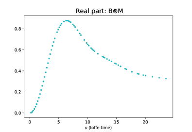
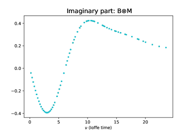
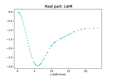
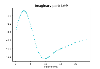
Figure 2.1: Upper plot: The NLO evolution term for the real (left) and imaginary part (right). Lower plot: The NLO scheme change term for the real (left) and imaginary part (right).

The evolution term $B\left(w\right)$ also connects pseudo-ITD points having different values of $z^{2}$: considering for example the real part, from Eqs. (2.3), (2.5) it follows

$$\text{Re}\left[\mathcal{M}\right]\left(\nu,z_{0}^{2}\right) =\text{Re}\left[\mathcal{M}\right]\left(\nu,z^{2}\right)$$

$$-C_{F}\frac{\alpha_{s}}{2\pi}\log\frac{z_{0}^{2}}{z^{2}}\int_{0}^{1}dx\,\left[\int_{0}^{1}dw\,B\left(w\right)\cos\left(x\nu w\right)\right]V_{3}\left(x,\mu^{2}\right)\,,$$ (2.9)

which relates the real part of the pseudo-ITD point at the scale $z^{2}$ with the one having the same Ioffe time at the scale $z_{0}^{2}$ Orginos:2017kos ; Karpie:2017bzm .

In the present work, we will consider the data for reduced pseudo-ITD from Refs. Joo:2019jct ; Joo:2020spy : the datasets presented in Ref. Joo:2019jct have been produced starting from three different lattice ensembles, denoted as fine, big and coarse and which differ for the volume and lattice spacing used in the simulations. They have been produced using values of the pion mass ranging from 358 MeV (fine) to 415 MeV (coarse and big). In the present work we will focus on the datapoints produced from the fine ensemble, while those from the coarse and big ones will be used to estimate systematic effects due to continuum limit and finite lattice volume. We will also consider pseudo-ITD points presented in Ref. Joo:2020spy , produced using pion mass equal to 172 MeV. Following the original convention of Ref. Joo:2020spy we will denote the corresponding lattice ensemble as 170. Points from the ensemble 280, presented in the same paper and produced using similar lattice spacing and pion mass 278 MeV, will be used to estimate the pion mass effects in the analyses for the ensembles fine and 170. These five ensembles of $2+1$ flavor lattice QCD were generated by the JLab/W&M collaboration using clover Wilson fermions and a tree level tadpole-improved Symanzik gauge action. One iteration of stout smearing with the weight $\rho=0.125$ for the staples is used in the fermion action. A direct consequence of the stout smearing is that the value of the tadpole corrected tree-level clover coefficient $c_{\rm SW}$ used is very close to the non-perturbative value determined, a posteriori, using the Schrödinger functional method. The detailed features of these ensembles are reported in Tab. 2.1, together with the number of reduced pseudo-ITD datapoints $n_{\text{dat}}$ computed from each of them.

Lattice ensemble	a(fm)	$M_{\pi}$ (MeV)	$L^{3}\times T$	$n_{\rm dat}$	Reference
fine	0.094(1)	358(3)	$32^{3}\times 64$	48
big	0.127(2)	415(23)	$32^{3}\times 96$	48	Joo:2019jct ; Joo:2020spy
coarse	0.127(2)	415(23)	$24^{3}\times 64$	36
280	0.094(1)	278(3)	$32^{3}\times 64$	64	Joo:2020spy
170	0.091(1)	172(6)	$64^{3}\times 128$	80

Table 2.1: Lattice data details

Given a set of lattice data for the real and imaginary part of the reduced pseudo-ITD, the distributions $T_{3}$ and $V_{3}$ can be extracted from them through a standard minimum-$\chi^{2}$ fit, following the approach described in Refs. Cichy2019 ; DelDebbio:2020cbz : the unknown $x$-dependence of the PDFs is parameterized at the chosen scale $\mu^{2}$, using a suitable parametric form, whose best parameters are determined minimizing the $\chi^{2}$ built using Eqs. (2.3), (2.4) and the corresponding lattice results. In this work we will perform this exercise using the NNPDF fitting framework, running the same machinery commonly used to extract PDFs from experimental data, already applied to lattice results in Ref. Cichy2019 . In the following we briefly recall its main relevant features, referring to Ref. Cichy2019 for more details.

The $x$-dependence of the distributions $f_{q}\left(x\right)$ ($V_{3}$ and $T_{3}$ in our case) is parameterized through a neural network $\text{NN}_{q}$ multiplied by a preprocessing polynomial factor, as

$$f_{q}\left(x\right)=x^{\alpha_{q}}\left(1-x\right)^{\beta_{q}}\text{NN}_{q}\left(x\right)\,,$$ (2.10)

$\alpha_{q},\beta_{q}$ being additional free parameters to be determined during the fit, alongside the weights and biases defining the neural network. Denoting the free parameters of the model as $\theta$, the best fit is determined minimizing the $\chi^{2}$ function, defined as

$$\chi^{2}\left(\theta\right)=\frac{1}{N_{\text{dat}}}\sum_{i,j}\left(\mathcal{O}\left(z_{i}\right)-\mathcal{O}^{\text{th}}\left(z_{i},\theta\right)\right)\left[\text{Cov}^{-1}\right]_{\text{ij}}\left(\mathcal{O}\left(z_{j}\right)-\mathcal{O}^{\text{th}}\left(z_{j},\theta\right)\right),$$ (2.11)

where $\mathcal{O}\left(z_{i}\right)$ denotes the measured lattice observable and $\mathcal{O}^{\text{th}}\left(z_{i},\theta\right)$ is the corresponding theoretical prediction, expressed using the matching coefficients of Eqs. (2.5), (2.6) and the parameterized parton distribution of Eq. (2.10). The implementation of the convolution entering Eqs. (2.3), (2.4) is performed by means of FastKernel tables, introduced and validated in Refs. Ball:2010de ; Bertone:2016lga in the context of global QCD fits, and currently used within the NNPDF code to obtain all the required theoretical predictions in a global fit. The covariance matrix entering Eq. (2.11) describes the distribution of the data, and takes into account the statistical and systematic uncertainties and their correlations. Considering $N_{c}$ independent sources of correlated systematics, its explicit expression is given by

$$\left[\text{Cov}\right]_{\text{ij}}=\delta_{ij}\left(\sigma^{\text{stat}}_{i,s}\right)^{2}+\sum_{l=1}^{N_{c}}\sigma^{\text{sys}}_{i,l}\sigma^{\text{sys}}_{j,l}\,,$$ (2.12)

where $\sigma^{\text{stat}}_{i}$ and $\sigma^{\text{sys}}_{i,l}$ represent the statistical and the l-th correlated systematic uncertainty of the i-th point.

The covariance matrix defined in Eq. (2.12) enters both the definition of the $\chi^{2}$ and the generation of Monte Carlo replicas Ball:2014uwa , being therefore important for both the central value of the fit and the final PDFs error. A solid knowledge of the covariance matrix is therefore an essential ingredient to get reliable results. The minimization of the $\chi^{2}$ is performed numerically: different algorithms can be implemented, here the CMA algorithm DBLP:journals/corr/Hansen16a is used, employing a cross-validation technique to avoid overfitting. The specific code used in the present work is the one employed for the production of the PDFs set NNPDF31 Ball:2017nwa , together with the ReportEngine software zahari_kassabov_2019_2571601 .

The NNPDF methodology has been used to produce PDF sets for many years now, and provides a flexible environment within which it has been possible to fit more than 4000 experimental points, coming from a variety of different high energy processes in different kinematic ranges Ball:2017nwa ; Ball:2014uwa . Therefore it represents a reliable framework which can be used to study and analyze the available lattice data, to assess how well these are able to constrain the PDFs and to compare lattice results with those coming from standard PDF sets. It is important to emphasise once again that in this analysis, once the FastKernel tables have been generated, the lattice data are treated exactly on the same footing as any other data, viz. the exact same methodology and code are used for fitting experimental and lattice data.

3 Fits over lattice data: statistical uncertainties only

In this section, we will present results for fits performed over the lattice data computed from the ensembles fine and 170, denoted as fine-stat and 170-stat respectively. Such fits have been produced considering statistical uncertainties only. We will show how, in general, without having the complete information regarding the lattice systematic uncertainties it is not always possible to obtain a good fit. In the next section, taking as example the case of the fine ensemble, we will discuss and estimate some of the possible systematic effects, studying their impact on the fit quality and on the resulting PDFs.

Parton distributions resulting from fits fine-stat and 170-stat, together with the corresponding error bands, are plotted in the upper and lower plots of Fig. 3.1, and the $\chi^{2}$ values are reported in Tab. 3.1: despite the PDFs extracted from the two datasets are compatible within one $\sigma$, the error band of the fit fine-stat appears to be slightly smaller than the other, with an average $\chi^{2}$ value per datapoint equal to $8.36$, pointing out a possible underestimation of the error and a bad fit quality. This could be caused by inconsistencies between different datapoints, due to unknown systematic uncertainties affecting them. On the other hand, the fit 170-stat shows better $\chi^{2}$ values, with an average value per datapoint equal to $1.38$.

Focusing on the more problematic case of the fine ensemble results, in order to assess which points are more likely to be affected by large systematic errors, we will study the contribution to the $\chi^{2}$ coming from each datapoint

$$\delta_{i}=\frac{\left(D_{i}-T_{i}\right)^{2}}{\sigma_{i}^{2}}\,,$$ (3.1)

$D_{i}$ and $T_{i}$ being the $i$-th lattice point and the corresponding prediction from the fit respectively, and find out which points $D_{i}$ are more than $4\sigma$ (or $3\sigma$) off from the fitted distribution $T_{i}$. These are the points that, most likely, do not belong to the fitted distribution and which therefore might be affected by larger systematic effects.

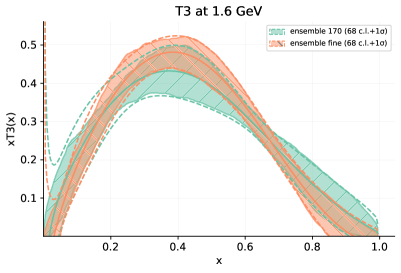
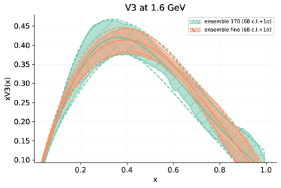
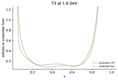
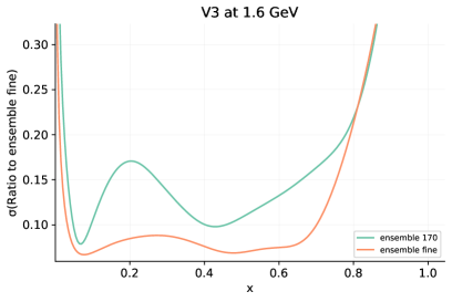
Figure 3.1: Upper plots: PDFs from datapoints computed from the ensembles fine and 170. The shaded bands represent the PDFs error computed as the 68 c.l. of the fit replicas, while the dashed line is obtained by computing the standard deviation point by point in $x$. Lower plots: corresponding PDFs errors, computed as standard deviation over fit replicas and displayed in function of $x$.

Ensemble	fit	Obs	$n_{\rm dat}$	$\chi^{2}$	$\chi^{2}_{tot}$
fine	fine-stat	$\text{Re}\left[\mathfrak{M}\right]$	48	7.94	8.36
		$\text{Im}\left[\mathfrak{M}\right]$	48	8.77
	fine-stat-$4\sigma$	$\text{Re}\left[\mathfrak{M}\right]$	39	2.68	3.28
		$\text{Im}\left[\mathfrak{M}\right]$	39	3.89
	fine-stat-$3\sigma$	$\text{Re}\left[\mathfrak{M}\right]$	34	1.45	1.86
		$\text{Im}\left[\mathfrak{M}\right]$	32	2.27
170	170-stat	$\text{Re}\left[\mathfrak{M}\right]$	80	0.68	1.38
		$\text{Im}\left[\mathfrak{M}\right]$	80	2.07

Table 3.1: Details of fits with statistical uncertainties only. From left to right we report the lattice ensemble, the fit name, the observables included in the analysis, the number of datapoints and finally the partial and total $\chi^{2}$.

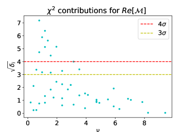
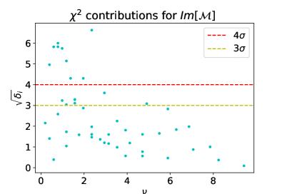
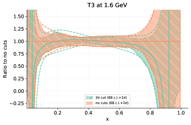
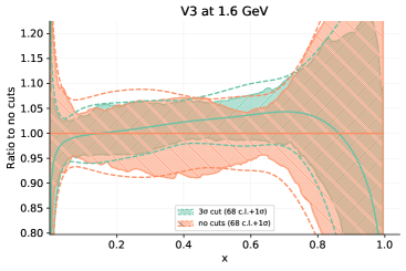
Figure 3.2: Upper plots: $\sqrt{\delta_{i}}$ contributions for each datapoint of the fine ensemble. The red and yellow lines highlight the $4\sigma$ and $3\sigma$ cut respectively. Lower plots: PDFs from fits fine-stat (orange) and fine-stat-3$\sigma$ (green), normalized to the former.

The contributions $\sqrt{\delta_{i}}$ are plotted in the upper plot of Fig. 3.2 as a function of the Ioffe-time $\nu$, with the red and yellow lines highlighting the $4\sigma$ and $3\sigma$ cut respectively: it is clear that a bunch of points having small Ioffe-time values are those giving the highest contribution to the total $\chi^{2}$, being more than $3\sigma$ or $4\sigma$ off. We can implement $4\sigma$ and $3\sigma$ cuts, removing the problematic points from the dataset and producing new fits, denoted as fine-stat-$3\sigma$ and fine-stat-$4\sigma$: the new fits show more reasonable $\chi^{2}$ values, reported in Tab. 3.1, showing how, upon removing the outliers, the remaining points, coming from a wide range of momentum $p$ and Euclidean separation $z_{3}$, are fitted reasonably well. The PDFs resulting from the $3\sigma$ cut are plotted in the lower plot of Fig. 3.2, normalized to the fit without any cuts: it is clear how, despite spoiling the total $\chi^{2}$, the problematic points do not seem to have a big impact on the final PDFs.

We conclude that, depending on the specific lattice ensemble we consider, quite a high number of small Ioffe-time points do not belong to the fitted distribution. In order to get reasonable $\chi^{2}$ values, such points have to be removed from the fit. This highlights possible tensions between datapoints and may point out the presence of systematic effects. In order to avoid any underestimation of the PDFs error and to introduce back in the analysis all the available points, systematic uncertainties need to be quantified and implemented in the fit.

4 Systematic effects

4.1 Discussion

The high $\chi^{2}$ values of the fits presented in the previous section might point out the presence of some tensions between datapoints. In the following, focusing on the case of the fine ensemble results, we will show that this is indeed the case, and we will investigate possible sources of systematic uncertainties and their numerical values.

The matrix element defining the pseudo-ITD is a function of the Ioffe-time $\nu$ and of the scale $z^{2}$. Points having the same Ioffe-time but different Euclidean separation can be related through Eq. (2), which can be used to evolve each pseudo-ITD point up to a chosen reference scale $z_{0}^{2}=\left(0.7\,a\right)^{2}$. Looking at Fig. 2.1 it is clear that, given this choice for $z_{0}$, the sign of the NLO correction of Eq. (2) will be positive for every datapoint, so that the evolution increases the real part of the pseudo-ITD. Considering the imaginary part, the sign of the NLO evolution term is initially negative, and it turns positive at bigger values of $\nu$. Such effects can be seen in Fig. 4.1, where the pseudo-ITD points computed from the fine ensemble are plotted before (blue) and after evolution (red).

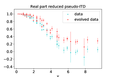
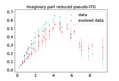
Figure 4.1: Data for the real part of the pseudo-ITD at their original scale $z^{2}$ and evolved at the common scale $z_{0}^{2}$.

After evolution, points having the same Ioffe time should have the same value. In practice, they should be compatible within errors. Looking at the red points of Fig. 4.1, where each point is plotted with the corresponding statistical uncertainty, it is clear how, expecially in the small Ioffe time region, this is not always the case: after evolution, some points having the same Ioffe time are not compatible between each other. Such discrepancies might be explained by the presence of systematic effects we are not accounting for.

A proper investigation of the systematic effects affecting the computation of the equal time correlators underlying the definition of pseudo-PDFs is a difficult and expensive task which would require to run different lattice simulations varying a set of parameters, like for example the lattice spacing, the lattice volume, the pion mass. Alongside systematic effects due to the lattice simulation, other sources of errors are those connected to the theoretical framework of the pseudo-PDFs approach, like the presence of higher twist effects and perturbative matching truncation effects. A detailed discussion of many of these uncertainties, together with a series of possible scenarios for their numerical values, can be found for example in Ref. Cichy2019 .

As mentioned in Sec. 2, in Ref. Joo:2019jct additional pseudo-ITD points were computed starting from other two lattice ensembles, with pion mass similar to that of the fine one, but having different volume and lattice spacing, denoted as big and coarse, whose features are reported in Tab. 2.1. Systematic uncertainties due to the continuum limit (CL) and finite volume (FV) can be directly estimated using these additional results as detailed in Ref. Joo:2019jct : the real and imaginary components of the pseudo-ITD are fitted to a polynomial as a function of the Ioffe-time $\nu$; the difference between coarse and fine ensemble results is taken as an estimate for lattice spacing effects as a function of $\nu$, while the analogous difference considering the coarse and big ensembles gives an estimate for uncertainties due to finite lattice volume. Systematic effects due to the pion mass (PM) can be estimated in a similar way: as mentioned in Sec. 2, in Ref. Joo:2020spy the data of the ensembles fine and 170 have been supplemented with additional pseudo-ITD results produced from a third ensemble having pion mass equal to $278$ MeV, denoted as ensemble 280. The difference between polynomial fits for the ensembles fine and 280 is taken as an estimate for pion mass effects. These differences will be considered as three independent sources of correlated systematic, affecting each datapoint entering the analysis. They are shown in the upper plots of Fig. 4.2 as functions of the Ioffe-time, denoted as FV (finite volume), CL (continuum limit) and PM (pion mass).

It is important to understand whether or not these systematic uncertainties are enough to account for the discrepancies described at the beginning of the section. In the lower plots of Fig. 4.2 FV, CL and PM systematic effects are plotted for the relevant Ioffe-time values, together with the aforementioned discrepancies. Consistently with what observed previously, the latter seem to affect mostly low Ioffe-time points, which are also those for which the estimated systematics reach their minimum values. Therefore from Fig. 4.2 it follows that FV, CL and PM systematics cannot be considered responsible for the big contributions to the $\chi^{2}$ noted in the fits of the previous section. In other words, they are likely not enough to account for the observed discrepancies affecting low Ioffe-time points. It should be noted that a study of more than 2 ensembles for each systematic error may be necessary for a more definitive conclusion.

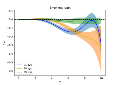
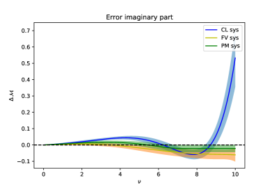
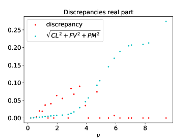
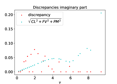
Figure 4.2: Upper plots: finite volume (FV), continuum limit (CL) and pion mass (PM) systematics provided as functions of the ioffe-time $\nu$ for the real (left) and imaginary (right) part of the matrix element. Lower plots: discrepancies between data having the same ioffe-time (red) together with the total FV, CL and PM systematic effects (blue).

Excited states contaminations might represent another possible source of systematic effects. Also missing higher orders in perturbation theory and higher twist effects could in principle be treated as additional systematic uncertainties. Unlike the case of the FV, CL and PM systematic uncertainties discussed above, we cannot estimate the size of such effects using the current lattice results. One could then follow the approach adopted in Ref. Cichy2019 , where different scenarios for the size of such systematics have been considered, and try to draw conclusions about their impact on the PDFs and on the fit quality. Here we will follow a different approach, trying to quantify an additional uncertainty which accounts for the unknown missing systematic effects, following a Bayesian approach as detailed in the following.

The figure of merit which is minimized during a Gaussian fit is defined as the probability of the data $D$ given the model parameters $\theta$, namely the likelihood

$$\mathcal{P}\left(D|\theta\right)=e^{-\frac{1}{2}\left(D-T\left(\theta\right)\right)^{T}\,\Sigma^{-1}\,\left(D-T\left(\theta\right)\right)}.$$ (4.1)

where $\Sigma$ is the covariance matrix of the data $D$, accounting for the known statistical and systematic uncertainties, and $T\left(\theta\right)$ is the theoretical prediction, function of the model parameters. If we assume the presence of unknown systematic effect $\Delta$ affecting the datapoints $D$, Eq. (4.1) can be modified as

$$\mathcal{P}\left(D,\Delta|\theta\right)=e^{-\frac{1}{2}\left(D+\Delta-T\left(\theta\right)\right)^{T}\,\Sigma^{-1}\,\left(D+\Delta-T\left(\theta\right)\right)}.$$ (4.2)

Assuming a Gaussian prior distribution $\mathcal{P}\left(\Delta\right)=\exp\left[-\frac{1}{2}\Delta^{T}\,\hat{\Sigma}^{-1}\,\Delta\right]$ we can marginalize over $\Delta$ getting

$$\int d\Delta\,\mathcal{P}\left(\Delta\right)\mathcal{P}\left(D,\Delta|\theta\right)\propto e^{-\frac{1}{2}\left(D-T\left(\theta\right)\right)\left(\Sigma+\hat{\Sigma}\right)^{-1}\left(D-T\left(\theta\right)\right)},$$ (4.3)

which defines the relevant likelihood to be minimized. Eq. (4.3) shows how the presence of unknown systematic effects can be accounted for by introducing in the likelihood an additional contribution to the covariance matrix, denoted by $\hat{\Sigma}$, which defines the prior probability distribution of these systematics. Its specific definition is of course arbitrary, and depends on the knowledge of the missing uncertainties we have.

This Bayesian approach, despite not providing a general method to estimate the missing systematics, allows to include in the analysis the partial information we may have about them. It should be noted that Eq. (4.3) is obtained under the hypothesis that the unknown systematic uncertainty is gaussianly distributed. This is an assumption of the model, often done in the literature, which allows to greatly simplify the problem. However depending on the specific data considered it might not be the most realistic one. In the present work we will work using this gaussian assumption, leaving for future studies the investigation of different choices for the prior probability distribution. A gaussian Bayesian approach has already been applied in different physical problems, when the data are affected by unknown sources of systematics: in the case of global QCD analysis, in Refs. AbdulKhalek:2019bux ; AbdulKhalek:2019ihb , a suitable covariance matrix $\hat{\Sigma}$ was defined by mean of scale variations, in order to take into account the theoretical error due to missing higher orders, while in Ref. Bernal:2018cxc a similar approach was applied to cosmological data.

In our case, we only know the discrepancies observed at the beginning of this section, not described by continuum limit, finite volume and pion mass effects. We can look at such discrepancies as an indication of the minimal size of the systematic effects affecting the data and use them to construct a suitable $\hat{\Sigma}$: for each couple of points having a given Ioffe-time value, we will define the two corresponding diagonal components of $\hat{\Sigma}$ as half of the distance between evolved points, setting the off diagonal elements to zero. Each point sharing the same Ioffe time value with at least another one will therefore be affected by an additional, uncorrelated systematic such that, after evolution, datapoints having the same Ioffe-time will be compatible between each other. Clearly, this global, uncorrelated systematic will be the dominant one for small Ioffe-time points, where most of the problematic points are, while for higher value of $\nu$ lattice spacing, finite volume and mass effects will dominate.

4.2 Results

To sum up, in Sec. 4.1, we have discussed and estimated four different source of systematics: the first three, accounting for finite volume, lattice spacing and pion mass effects, can be computed directly from the available lattice results as a function of the Ioffe-time $\nu$, and will be implemented in the fit as three independent sources of correlated systematics; the fourth one has been estimated using the size of the discrepancies observed between points having the same Ioffe-time, and will be considered as an additional uncorrelated uncertainty, in order to take into account the minimal size of all the remaining systematic effects we have not directly computed. As mentioned in Sec. 2, such systematics enter the definition of the covariance matrix responsible for both replicas generation and the $\chi^{2}$ definition, and therefore it has a central role in both the determination of the fit central value and its error band. The new fit is denoted as fine-sys and the resulting PDFs are plotted in Fig. 4.3, together with the results from the fit fine-stat presented Sec. 3: the distribution $T_{3}$ is only marginally affected by the introduction of the systematic errors, showing a mild down shift of its central value in the medium and large $x$ regions; on the other hand both the central value and the error band of $V_{3}$ change, with an overall down shift of the former and a sizable increase of the latter. The $\chi^{2}$ values are reported in Tab. 4.1: the average value per datapoint is now $1.15$, showing a good fit quality. It should be noted that after the inclusion of systematic uncertainties in the analysis, the effect on the final result could be different depending on the specific situation we are considering. In other words, it is not always the case that the inclusion of new systematic effects leads to an increase of the final PDFs error. This can be seen for example in the case of the distribution $T_{3}$ plotted in Fig. 4.3, from which it is clear how the error of the fit fine-sys has not increased with respect to the one of fine-stat. The reason for this can be traced back to the fact that the covariance matrix defined in Eq. (2.12) enters both the Monte Carlo replicas generation and the $\chi^{2}$ definition of Eq. (2.11): while the former mostly controls the final PDFs error, the latter is responsible for the relative weights different points have in the analysis. Points affected by bigger errors will give smaller contributions to the $\chi^{2}$ and therefore will count less in the fit. Each replica will be shifted by a certain amount, which takes into account both the new replicas distribution and the different weights of the data entering the $\chi^{2}$, so that the net effect on the final PDFs is non-trivial, and might consist in a global shift of the central value of the replicas distribution rather than in an increase of its error band.

Ensemble	fit	Obs	$n_{\rm dat}$	$\chi^{2}$	$\chi^{2}_{tot}$
fine	no cuts	$\text{Re}\left[\mathfrak{M}\right]$	48	1.00	1.15
		$\text{Im}\left[\mathfrak{M}\right]$	48	1.30

Table 4.1: Details of the fit with systematic uncertainties. From left to right we report the lattice ensemble, the fit name, the observables included in the analysis, the number of datapoints and finally the partial and total $\chi^{2}$.

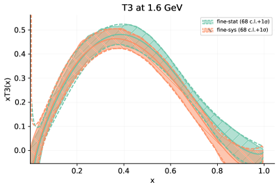
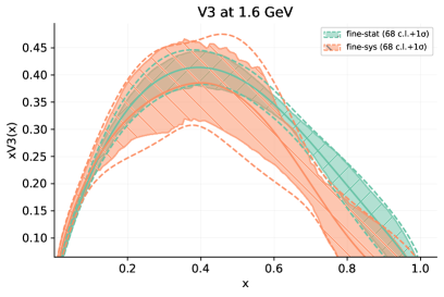
Figure 4.3: PDFs from the fits fine-stat and fine-sys.

Despite it is probably too early to draw comparisons between our results and phenomenological distributions, it is interesting to see how they look when plotted together: given the fact that nowadays $V_{3}$ and $T_{3}$ are very well constrained by experimental data, the discrepancies we observe between lattice and phenomenological results might be a good indication of the size of the systematic we are still missing, highlighting specific $x$-region where the lattice PDFs error might have been underestimated. In Fig. 4.4, our result fine-sys and the corresponding distributions from the NLO PDF sets NNPDF31 Ball:2017nwa are plotted together (orange and green curves respectively), both as absolute values (upper plots) and normalized to NNPDF31 (lower plots). Looking at results from fine-sys, in the case of both $V_{3}$ and $T_{3}$ the two distributions are compatible up to medium ($\sim 0.25$ and $\sim 0.45$) and for large values of $x$ ($>0.8$), showing a probable underestimation of the PDFs error for the intermediate $x$ ranges.

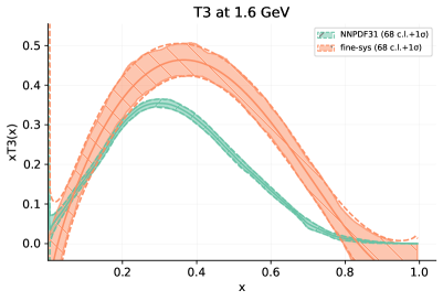
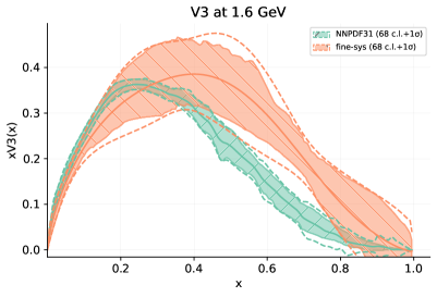
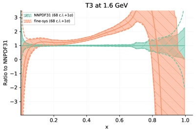
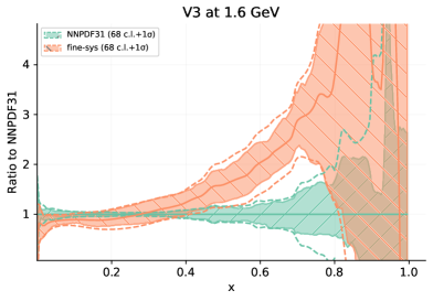
Figure 4.4: PDFs from the fits fine-sys compared with the corresponding distributions from NNPDF31. In the lower plots results are normalized to NNPDF31 PDFs.

5 Conclusions

In the present paper, we have considered the pseudo-ITD data produced in Refs. Joo:2019jct ; Joo:2020spy . Using the position space factorization theorem relating such data to collinear PDFs, we have extracted two nonsinglet distributions within the NNPDF framework.

After extracting PDFs from different data sets and considering statistical uncertainties only, we have shown that in one of the cases considered, the fit quality appears to be really poor, pointing out the need for a detailed knowledge of the systematic effects. Using the results of Ref. Joo:2019jct ; Joo:2020spy we have directly estimated those connected to finite volume, lattice spacing and pion mass effects. As for systematic uncertainties which cannot be directly computed from lattice results (like for example truncation effects and higher twist corrections), starting from the observed discrepancies between low Ioffe-time points we have used a Bayesian approach to introduce an additional systematic which allows us to mitigate the tensions between the problematic datapoints, using the partial pieces of information which are available to us.

The Bayesian approach however is not completely satisfying, since it relies on a partial knowledge of the missing uncertainties and requires to make a number of assumptions about them. More work has to be done to achieve a detailed knowledge of the systematic uncertainties in lattice simulations: without a stringent control over them, it is not possible to draw reliable conclusions and to make comparisons with phenomenological distributions.

Finally, we stress once more that the analysis performed in this paper is complementary to that presented in Ref. Cichy2019 , where quasi-PDFs matrix elements where considered instead, starting from the momentum space version of the factorization theorem. In both cases, results have been produced within the NNPDF environment, running the same machinery used for global QCD analysis over experimental data. The next logical step might be a global lattice QCD fit within this same framework, where data for multiple lattice observables coming from different simulations are simultaneously included in the analysis.

Appendix A Pion Mass dependence for 170 ensemble

Similarly to what done for the fine ensemble in Sec. 4.1, the data for the ensemble 280 presented in Ref. Joo:2020spy can also be used to estimate pion mass effects for results concerning the ensemble 170. The corresponding polynomial curves are plotted in Fig. A.1 as functions of the Ioffe-time.

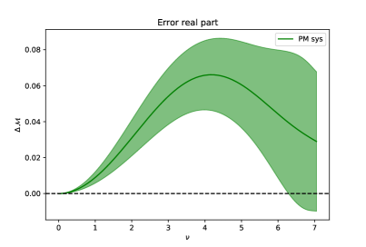
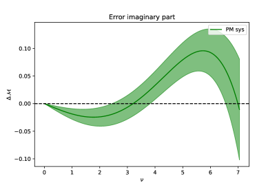
Figure A.1: Pion mass (PM) systematic provided as functions of the ioffe-time $\nu$ for the real (left) and imaginary (right) part of the matrix element.

As in the case of the analysis for the fine ensemble, the curves in Fig. A.1 are used to define a source of correlated systematic. The resulting PDFs, denoted as 170-sys, are plotted in Fig. A.2 together with the results for the ensemble 170 presented in Sec. 3, where only statistical uncertainties have been considered. From Fig. A.2 it is clear how introducing pion mass systematic effects in the analysis has very little impact on the distributions, the major effect being a mild down shift of the central value of $V_{3}$ in the medium $x$ region.

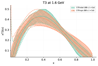
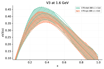
Figure A.2: PDFs from the fits 170-stat and 170-sys.

We conclude that the mild pion mass dependence observed in pseudo-ITD data of Ref. Joo:2020spy has no sizable impact on the final PDFs.

Appendix B Comparison with results from quasi-PDFs matrix elements

It is interesting to compare our best result fine-sys with the best result of Ref. Cichy2019 , denoted as nnpdf31_qpdf_S2. Both PDFs sets have been obtained using the same NNPDF methodology, the only difference being the input data (pesudo-ITD and quasi-PDFs data respectively) and the corresponding errors. For more details about the specific systematics uncertainties considered in the analysis for nnpdf31_qpdf_S2 we refer to the original publication Cichy2019 .

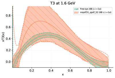
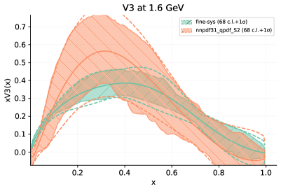
Figure B.1: PDFs from the fits fine-sys compared with the corresponding distributions from the fit nnpdf31_qpdf_S2, presented in Ref. Cichy2019 .

Quasi-PDFs and pseudo-ITD results are plotted together in Fig. B.1: both $T_{3}$ and $V_{3}$ distributions appear to be in good agreement, the main difference being a huge decrease in the PDFs error when considering results presented in this work. This difference can be partially traced back to the number of points included in the analysis: while in Ref. Cichy2019 16 points for quasi-PDFs matrix element where included, in the present work data corresponding to all momentum values are considered, for a total of 48 pseudo-ITD points. Clearly, having more points in the analysis allows to better constraint the fit results, giving final PDFs with smaller error. Given equivalent computational cost, the low momenta matrix elements, which are used in the pseudo-PDF approach, are exponentially more precise than the large momenta matrix elements, to which the quasi-PDF approach are restricted. The size of the statistical and systematic uncertainties affecting the points entering the two analyses is of course another reason for different PDFs error, however a detailed study of such differences is beyond the scope of this work. We leave a detailed comparison between the quasi- and pseudo-PDFs approaches for a future study.

References

- (1) NNPDF collaboration, Parton distributions from high-precision collider data, Eur. Phys. J. C77 (2017) 663 [1706.00428].
- (2) S. Dulat, T.-J. Hou, J. Gao, M. Guzzi, J. Huston, P. Nadolsky et al., New parton distribution functions from a global analysis of quantum chromodynamics, Phys. Rev. D93 (2016) 033006 [1506.07443].
- (3) S. Alekhin, J. Blümlein, S. Moch and R. Placakyte, Parton distribution functions, , and heavy-quark masses for LHC Run II, Phys. Rev. D96 (2017) 014011 [1701.05838].
- (4) A. D. Martin, W. J. Stirling, R. S. Thorne and G. Watt, Parton distributions for the LHC, Eur. Phys. J. C63 (2009) 189 [0901.0002].
- (5) A. Buckley, J. Ferrando, S. Lloyd, K. Nordström, B. Page, M. Rüfenacht et al., LHAPDF6: parton density access in the LHC precision era, Eur. Phys. J. C75 (2015) 132 [1412.7420].
- (6) M. Constantinou et al., Parton distributions and lattice QCD calculations: toward 3D structure, 2006.08636.
- (7) M. Constantinou, The x-dependence of hadronic parton distributions: A review on the progress of lattice QCD, 10, 2020, 2010.02445.
- (8) A. Radyushkin, Theory and applications of parton pseudodistributions, Int. J. Mod. Phys. A 35 (2020) 2030002 [1912.04244].
- (9) K. Cichy and M. Constantinou, A guide to light-cone PDFs from Lattice QCD: an overview of approaches, techniques and results, Adv. High Energy Phys. 2019 (2019) 3036904 [1811.07248].
- (10) C. Monahan, Recent Developments in -dependent Structure Calculations, PoS LATTICE2018 (2018) 018 [1811.00678].
- (11) X. Ji, Y.-S. Liu, Y. Liu, J.-H. Zhang and Y. Zhao, Large-Momentum Effective Theory, 2004.03543.
- (12) X. Ji, Parton physics on a euclidean lattice, Phys. Rev. Lett. 110 (2013) 262002.
- (13) A. V. Radyushkin, Quasi-parton distribution functions, momentum distributions, and pseudo-parton distribution functions, Phys. Rev. D96 (2017) 034025 [1705.01488].
- (14) B. U. Musch, P. Hagler, J. W. Negele and A. Schafer, Exploring quark transverse momentum distributions with lattice QCD, Phys. Rev. D 83 (2011) 094507 [1011.1213].
- (15) V. Braun, P. Gornicki and L. Mankiewicz, Ioffe - time distributions instead of parton momentum distributions in description of deep inelastic scattering, Phys. Rev. D51 (1995) 6036 [hep-ph/9410318].
- (16) X. Ji, J.-H. Zhang and Y. Zhao, Renormalization in Large Momentum Effective Theory of Parton Physics, Phys. Rev. Lett. 120 (2018) 112001 [1706.08962].
- (17) T. Ishikawa, Y.-Q. Ma, J.-W. Qiu and S. Yoshida, Renormalizability of quasiparton distribution functions, Phys. Rev. D96 (2017) 094019 [1707.03107].
- (18) A. V. Radyushkin, Quark pseudodistributions at short distances, Phys. Lett. B781 (2018) 433 [1710.08813].
- (19) A. Radyushkin, Nonperturbative Evolution of Parton Quasi-Distributions, Phys. Lett. B767 (2017) 314 [1612.05170].
- (20) T. Izubuchi, X. Ji, L. Jin, I. W. Stewart and Y. Zhao, Factorization Theorem Relating Euclidean and Light-Cone Parton Distributions, Phys. Rev. D98 (2018) 056004 [1801.03917].
- (21) X. Ji, J.-H. Zhang and Y. Zhao, More On Large-Momentum Effective Theory Approach to Parton Physics, Nucl. Phys. B924 (2017) 366 [1706.07416].
- (22) L. Del Debbio, T. Giani and C. J. Monahan, Notes on lattice observables for parton distributions: nongauge theories, 2007.02131.
- (23) Y.-Q. Ma and J.-W. Qiu, Exploring Partonic Structure of Hadrons Using ab initio Lattice QCD Calculations, Phys. Rev. Lett. 120 (2018) 022003 [1709.03018].
- (24) Y.-Q. Ma and J.-W. Qiu, Extracting Parton Distribution Functions from Lattice QCD Calculations, Phys. Rev. D98 (2018) 074021 [1404.6860].
- (25) J. Karpie, K. Orginos, A. Rothkopf and S. Zafeiropoulos, Reconstructing parton distribution functions from ioffe time data: from bayesian methods to neural networks, Journal of High Energy Physics 2019 (2019) 57.
- (26) T. Izubuchi, L. Jin, C. Kallidonis, N. Karthik, S. Mukherjee, P. Petreczky et al., Valence parton distribution function of pion from fine lattice, 1905.06349.
- (27) K. Cichy, L. Del Debbio and T. Giani, Parton distributions from lattice data: the nonsinglet case, Journal of High Energy Physics 2019 (2019) 137.
- (28) X. Gao, L. Jin, C. Kallidonis, N. Karthik, S. Mukherjee, P. Petreczky et al., Valence parton distribution of pion from lattice QCD: Approaching continuum, 2007.06590.
- (29) C. Alexandrou, K. Cichy, M. Constantinou, K. Jansen, A. Scapellato and F. Steffens, Light-Cone Parton Distribution Functions from Lattice QCD, Phys. Rev. Lett. 121 (2018) 112001 [1803.02685].
- (30) C. Alexandrou, K. Cichy, M. Constantinou, K. Hadjiyiannakou, K. Jansen, A. Scapellato et al., Systematic uncertainties in parton distribution functions from lattice QCD simulations at the physical point, Phys. Rev. D99 (2019) 114504 [1902.00587].
- (31) J. Bringewatt, N. Sato, W. Melnitchouk, J.-W. Qiu, F. Steffens and M. Constantinou, Confronting lattice parton distributions with global QCD analysis, 2010.00548.
- (32) B. Joó, J. Karpie, K. Orginos, A. Radyushkin, D. Richards and S. Zafeiropoulos, Parton Distribution Functions from Ioffe time pseudo-distributions, JHEP 12 (2019) 081 [1908.09771].
- (33) B. Joó, J. Karpie, K. Orginos, A. V. Radyushkin, D. G. Richards and S. Zafeiropoulos, Parton Distribution Functions from Ioffe time pseudo-distributions from lattice caclulations; approaching the physical point, 2004.01687.
- (34) H.-W. Lin, J.-W. Chen, S. D. Cohen and X. Ji, Flavor Structure of the Nucleon Sea from Lattice QCD, Phys. Rev. D91 (2015) 054510 [1402.1462].
- (35) J.-W. Chen, S. D. Cohen, X. Ji, H.-W. Lin and J.-H. Zhang, Nucleon Helicity and Transversity Parton Distributions from Lattice QCD, Nucl. Phys. B911 (2016) 246 [1603.06664].
- (36) C. Alexandrou, K. Cichy, V. Drach, E. Garcia-Ramos, K. Hadjiyiannakou, K. Jansen et al., Lattice calculation of parton distributions, Phys. Rev. D92 (2015) 014502 [1504.07455].
- (37) C. Alexandrou, K. Cichy, M. Constantinou, K. Hadjiyiannakou, K. Jansen, F. Steffens et al., Updated Lattice Results for Parton Distributions, Phys. Rev. D96 (2017) 014513 [1610.03689].
- (38) C. Monahan and K. Orginos, Quasi parton distributions and the gradient flow, JHEP 03 (2017) 116 [1612.01584].
- (39) J.-H. Zhang, J.-W. Chen, X. Ji, L. Jin and H.-W. Lin, Pion Distribution Amplitude from Lattice QCD, Phys. Rev. D95 (2017) 094514 [1702.00008].
- (40) C. Alexandrou, K. Cichy, M. Constantinou, K. Hadjiyiannakou, K. Jansen, H. Panagopoulos et al., A complete non-perturbative renormalization prescription for quasi-PDFs, Nucl. Phys. B923 (2017) 394 [1706.00265].
- (41) J. Green, K. Jansen and F. Steffens, Nonperturbative Renormalization of Nonlocal Quark Bilinears for Parton Quasidistribution Functions on the Lattice Using an Auxiliary Field, Phys. Rev. Lett. 121 (2018) 022004 [1707.07152].
- (42) J.-W. Chen, L. Jin, H.-W. Lin, Y.-S. Liu, Y.-B. Yang, J.-H. Zhang et al., Lattice Calculation of Parton Distribution Function from LaMET at Physical Pion Mass with Large Nucleon Momentum, 1803.04393.
- (43) C. Alexandrou, K. Cichy, M. Constantinou, K. Jansen, A. Scapellato and F. Steffens, Transversity parton distribution functions from lattice QCD, Phys. Rev. D. (Rapid Communication), in production, (2018) [1807.00232].
- (44) H.-W. Lin, J.-W. Chen, X. Ji, L. Jin, R. Li, Y.-S. Liu et al., Proton Isovector Helicity Distribution on the Lattice at Physical Pion Mass, Phys. Rev. Lett. 121 (2018) 242003 [1807.07431].
- (45) Z.-Y. Fan, Y.-B. Yang, A. Anthony, H.-W. Lin and K.-F. Liu, Gluon Quasi-Parton-Distribution Functions from Lattice QCD, Phys. Rev. Lett. 121 (2018) 242001 [1808.02077].
- (46) Y.-S. Liu, J.-W. Chen, L. Jin, R. Li, H.-W. Lin, Y.-B. Yang et al., Nucleon Transversity Distribution at the Physical Pion Mass from Lattice QCD, 1810.05043.
- (47) J. R. Green, K. Jansen and F. Steffens, Improvement, generalization, and scheme conversion of Wilson-line operators on the lattice in the auxiliary field approach, Phys. Rev. D 101 (2020) 074509 [2002.09408].
- (48) Y. Chai et al., Parton distribution functions of on the lattice, Phys. Rev. D 102 (2020) 014508 [2002.12044].
- (49) H.-W. Lin, J.-W. Chen, Z. Fan, J.-H. Zhang and R. Zhang, The Valence-Quark Distribution of the Kaon from Lattice QCD, 2003.14128.
- (50) C. Alexandrou, K. Cichy, M. Constantinou, K. Hadjiyiannakou, K. Jansen, A. Scapellato et al., Unpolarized and helicity generalized parton distributions of the proton within lattice QCD, 2008.10573.
- (51) K. Orginos, A. Radyushkin, J. Karpie and S. Zafeiropoulos, Lattice QCD exploration of parton pseudo-distribution functions, Phys. Rev. D96 (2017) 094503 [1706.05373].
- (52) J. Karpie, K. Orginos and S. Zafeiropoulos, Moments of Ioffe time parton distribution functions from non-local matrix elements, JHEP 11 (2018) 178 [1807.10933].
- (53) B. Joó, J. Karpie, K. Orginos, A. V. Radyushkin, D. G. Richards, R. S. Sufian et al., Pion valence structure from Ioffe-time parton pseudodistribution functions, Phys. Rev. D 100 (2019) 114512 [1909.08517].
- (54) M. Bhat, K. Cichy, M. Constantinou and A. Scapellato, Parton distribution functions from lattice QCD at physical quark masses via the pseudo-distribution approach, 2005.02102.
- (55) Z. Fan, R. Zhang and H.-W. Lin, Nucleon Gluon Distribution Function from 2+1+1-Flavor Lattice QCD, 2007.16113.
- (56) G. S. Bali et al., Pion distribution amplitude from Euclidean correlation functions, Eur. Phys. J. C78 (2018) 217 [1709.04325].
- (57) G. S. Bali, V. M. Braun, B. Gläßle, M. Göckeler, M. Gruber, F. Hutzler et al., Pion distribution amplitude from Euclidean correlation functions: Exploring universality and higher-twist effects, Phys. Rev. D 98 (2018) 094507 [1807.06671].
- (58) R. S. Sufian, J. Karpie, C. Egerer, K. Orginos, J.-W. Qiu and D. G. Richards, Pion Valence Quark Distribution from Matrix Element Calculated in Lattice QCD, Phys. Rev. D99 (2019) 074507 [1901.03921].
- (59) RQCD collaboration, Light-cone distribution amplitudes of octet baryons from lattice QCD, Eur. Phys. J. A 55 (2019) 116 [1903.12590].
- (60) R. S. Sufian, C. Egerer, J. Karpie, R. G. Edwards, B. Joó, Y.-Q. Ma et al., Pion Valence Quark Distribution from Current-Current Correlation in Lattice QCD, 2001.04960.
- (61) A. Radyushkin, One-loop evolution of parton pseudo-distribution functions on the lattice, Phys. Rev. D98 (2018) 014019 [1801.02427].
- (62) J. Karpie, K. Orginos, A. Radyushkin and S. Zafeiropoulos, Parton distribution functions on the lattice and in the continuum, EPJ Web Conf. 175 (2018) 06032 [1710.08288].
- (63) R. D. Ball, L. Del Debbio, S. Forte, A. Guffanti, J. I. Latorre, J. Rojo et al., A first unbiased global NLO determination of parton distributions and their uncertainties, Nucl. Phys. B838 (2010) 136 [1002.4407].
- (64) V. Bertone, S. Carrazza and N. P. Hartland, APFELgrid: a high performance tool for parton density determinations, Comput. Phys. Commun. 212 (2017) 205 [1605.02070].
- (65) NNPDF collaboration, Parton distributions for the LHC Run II, JHEP 04 (2015) 040 [1410.8849].
- (66) N. Hansen, The CMA evolution strategy: A tutorial, CoRR abs/1604.00772 (2016) [1604.00772].
- (67) Z. Kassabov, “Reportengine: A framework for declarative data analysis.” https://doi.org/10.5281/zenodo.2571601, Feb., 2019. 10.5281/zenodo.2571601.
- (68) NNPDF collaboration, A First Determination of Parton Distributions with Theoretical Uncertainties, 1905.04311.
- (69) NNPDF collaboration, Parton Distributions with Theory Uncertainties: General Formalism and First Phenomenological Studies, 1906.10698.
- (70) J. Luis Bernal and J. A. Peacock, Conservative cosmology: combining data with allowance for unknown systematics, JCAP 07 (2018) 002 [1803.04470].
- (71) Jülich Supercomputing Centre, JURECA: Modular supercomputer at Jülich Supercomputing Centre, Journal of large-scale research facilities 4 (2018) .
- (72) SciDAC, LHPC, UKQCD collaboration, The Chroma software system for lattice QCD, Nucl. Phys. B Proc. Suppl. 140 (2005) 832 [hep-lat/0409003].
- (73) M. Clark, R. Babich, K. Barros, R. Brower and C. Rebbi, Solving Lattice QCD systems of equations using mixed precision solvers on GPUs, Comput. Phys. Commun. 181 (2010) 1517 [0911.3191].
- (74) R. Babich, M. A. Clark and B. Joo, Parallelizing the QUDA Library for Multi-GPU Calculations in Lattice Quantum Chromodynamics, in SC 10 (Supercomputing 2010), 11, 2010, 1011.0024.
- (75) F. Winter, M. Clark, R. Edwards and B. Joó, A Framework for Lattice QCD Calculations on GPUs, in 28th IEEE International Parallel and Distributed Processing Symposium, 8, 2014, 1408.5925, DOI.
- (76) B. Joó, D. D. Kalamkar, K. Vaidyanathan, M. Smelyanskiy, K. Pamnany, V. W. Lee et al., Lattice QCD on Intel®Xeon Phi Coprocessors, Lect. Notes Comput. Sci. 7905 (2013) 40.
- (77) B. Joó, D. D. Kalamkar, T. Kurth, K. Vaidyanathan and A. Walden, Optimizing wilson-dirac operator and linear solvers for intel® knl, in High Performance Computing, M. Taufer, B. Mohr and J. M. Kunkel, eds., (Cham), pp. 415–427, Springer International Publishing, 2016.