A Unified Combination of
Classical and Quantum Systems

Abstract

Any particular classical system and its quantum version are normally viewed as separate formulations that are strictly distinct. Our goal is to overcome the two separate languages and create a smooth and common procedure that provides a clear and continuous passage between the conventional distinction of either a strictly classical or a strictly quantized state. While path integration, among other procedures, provides an alternative route to connect classical and quantum expressions, it normally involves complicated, model-dependent, integrations. Our alternative procedures involve only model-independent procedures, and use more natural and straightforward integrations that are universal in kind. To introduce the basic procedures our presentation begins with familiar methods that are limited to basic, conventional, canonical quantum mechanical examples. In the final sections we illustrate how alternative quantization procedures, e.g., spin and affine quantizations, can also have smooth paths between classical and quantum stories, and with a few brief remarks, can also lead to similar stories for non-renormalizable covariant scalar fields as well as quantum gravity.

1 Introduction

1.1 Classical formulations

We start by describing phase space as a set of momenta ($p$) and coordinates ($q$), which have a measure ($dp\,dq$). Dynamical equations are time ($t$) dependent ($p(t)$) and ($q(t)$), which are dictated by stationary variations of a classical ($c$) action functional

$$A_{c}={\textstyle\int}_{0}^{T}\{p(t)\,\dot{q}(t)-H(p(t),q(t))\,\}\;dt\;,$$ (1)

that leads, with $\dot{q}(t)\equiv d\,q(t)/dt$, to

$$\delta A_{c}={\textstyle\int}_{0}^{T}\{[\dot{q}(t)-\partial H(p(t),q(t)/\partial p(t)]\,\delta p(t)$$

$$\hskip 50.00008pt-[\dot{p}(t)+\partial H(p(t),q(t))/\partial q(t)]\,\delta q(t)\}\;dt$$

$$\hskip 70.0001pt+q(t)\,\delta p(t)|_{0}^{T}-p(t)\,\delta q(t)|_{0}^{T}=0\;,$$ (2)

with arbitrary $\delta p(t)$ and $\delta q(t)$ values, except that $\delta p(T)=\delta p(0)=0$ and $\delta q(T)=\delta q(0)=0$. All this leads to the traditional classical equations of motion given by

$$\dot{q}(t) \hskip-13.00005pt=\partial\,H(p(t),q(t))/\partial p(t)\;,$$

$$\dot{p}(t) \hskip-13.00005pt=-\partial\,H(p(t),q(t))/\partial q(t)\;.$$ (3)

A common example is $H(p,q)=(p^{2}/m+m\,\omega^{2}q^{2})/2$, which is an harmonic oscillator, and its dynamical equations are given by $\dot{q}(t)=p(t)/m$ and $\dot{p}(t)=-m\,\omega^{2}q(t)$. It follows that $\ddot{q}(t)=-\omega^{2}q(t)$ with solutions $q(t)=q_{0}\cos(\omega\,t)+(p_{0}/m\,\omega)\sin(\omega\,t)$, where $q_{0}=q(0)$ and $p_{0}=p(0)$.

1.2 Quantum formulations

The basic quantum operators are linked with suitably chosen classical variables, i.e., $p\rightarrow P$ and $q\rightarrow Q$, which satisfy the rule $QP-PQ\equiv[Q,P]=i\hbar 1\!\!1$. Note: The rules used to choose the favored classical variables, $p$ and $q$, that are promoted to operators, $P$ and $Q$, are addressed below.

Various operators, such as ${\cal{W}}(P,Q)$, act upon suitable Hilbert space vectors, such as $|\Phi\rangle$ leading to new Hilbert space vectors, ${\cal{W}}(P,Q)|\Phi\rangle$. It is conventionally observed that the operator $Q$ is diagonalized when acting on selected eigenvectors. This leads to the relations that $Q|x\rangle=x|x\rangle$ while then $P|x\rangle=-i\hbar(\partial/\partial x)\,|x\rangle$. A general Hilbert space vector $|\Phi\rangle$ then becomes $\Phi(x)=\langle x|\Phi\rangle$, and the normalization of a general vector is $\langle\Phi|\Phi\rangle={\textstyle\int}|\Phi(x)|^{2}\;dx<\infty$. While such relations formally are correct, it should be recognized that $|x\rangle$ is strictly not a proper Hilbert space vector since $\langle x|x\rangle=\infty$ as follows from the fact that $\langle x^{\prime}|x\rangle=\delta(x^{\prime}-x)$.

The algebra of quantum operators, such as the self-adjoint Hamiltonian operator ${\cal H}(P,Q)$, act upon vectors from a suitable Hilbert space. Such vectors as $|\Phi\rangle$ are finite in normalization, as denoted by $\langle\Phi|\Phi\rangle<\infty$. Indeed, normalized vectors, which means that $\langle\Phi|\Phi\rangle=1$, play an important role. Quantum dynamics is expressed by time dependence of the vectors, e.g., $|\Phi(t)\rangle$. The quantum ($q$) action functional involves normalized vectors, and is given by

$$A_{q}={\textstyle\int}_{0}^{T}\langle\Phi(t)|[i\hbar\,(\partial/\partial t)-{\cal H}(P,Q)]|\Phi(t)\rangle\;dt\;,$$ (4)

and stationary variations of the quantum action functional lead to

$$\delta A_{q}={\textstyle\int}_{0}^{T}\{\delta\langle\Phi(t)|[i\hbar\,(\partial/\partial t)-{\cal H}(P,Q)]|\Phi(t)\rangle\;$$

$$\hskip 50.00008pt+\langle\Phi(t)|[i\hbar\,(\partial/\partial t)-{\cal H}(P,Q)]\,\delta|\Phi(t)\rangle\,\}\;dt=0\;.$$ (5)

This leads to two equations, one of which is

$$i\hbar(\partial\,|\Phi(t)\rangle/\partial t)={\cal H}(P,Q)\,|\Phi(t)\rangle\;,$$ (6)

which is a version of ‘Schrödinger’s equation’ [1]; the second equation is the adjoint of the first equation.

The basic operators, $P$ and $Q$, can generate various additional operators, such as an harmonic oscillator given by ${\cal H}(P,Q)=(P^{2}/m+m\,\omega^{2}Q^{2})/2$. For the Hilbert space ‘vectors’ $|x\rangle$, defined by $Q|x\rangle=x|x\rangle$, the ground-state eigenvector of the harmonic oscillator is $\langle x|\omega\rangle={\cal{N}}\exp[-m\,\omega\,x^{2}/2\hbar]$, i.e., namely a familiar Gaussian function.

2 Coherent States

2.1 Choosing the correct quantum operators

Since classical mechanics has a long history, it is natural that the classical variables are chosen before choosing what quantum operators to employ. That behavior has its natural difficulties because while there are many acceptable classical variables $p$ and $q$, or $\overline{p}$ and $\overline{q}$, etc., provided the Hamiltonian function also is changed so that $\overline{p}=\overline{p}(p,q)$ and $\overline{q}=\overline{q}(p,q)$, along with the Poisson brackets $\{p,q\}=\{\overline{p},\overline{q}\}=1$, which leads to $\overline{H}(\overline{p},\overline{q})=H(p,q)$ for all variables.

On the other hand, a promotion of classical variables to quantum operators, such as $p\rightarrow P$ and $q\rightarrow Q$, but generally, $\overline{H}(\overline{P},\overline{Q})\neq H(P,Q)$, and when the Hamiltonian operators are different, they definitely can lead to different physics. It is absolutely necessary to find a procedure whereby favored classical variables are the ones that are promoted to the correct quantum operators. Accepting an arbitrary choice of canonical variables to promote to quantum operators would most likely lead to a false quantization procedure. How a correct choice of canonical variables to promote to quantum operators can be made is the subject of this subsection.

Dirac [2] has offered the clue to the task ahead. He claimed that the favored classical variables, $p$ and $q$, are those that obey the relation $H(p,q)\rightarrow H(P,Q)$, i.e., the classical functional form equals the quantum functional form, and moreover, the classical variables must also be Cartesian coordinates, a rule that necessarily implies that $-\infty<p,q<\infty$. At the first glance this seems impossible because phase space $-$ the home of the variables $p$ and $q$ $-$ has no metric to determine Cartesian coordinates. Dirac did not propose how to find such coordinates, but the author has recently found a suitable procedure to do just that. That story is published in [3], and is recast here below.

To seek Cartesian coordinates we first choose a family of canonical coherent states. We start by choosing $P$ and $Q$, such that $[Q,P]=i\hbar 1\!\!1$, and a pair of classical variables $p$ and $q$. For our coherent states we choose Hilbert space vectors such as

$$|p,q\rangle\equiv e^{-iqP/\hbar}\,e^{ipQ/\hbar}|\omega\rangle\;,$$ (7)

where it is customary that $(Q+iP/\omega)\,|\omega\rangle=0$; this choice will also play an important role later. It follows that $\langle\omega|(Q+iP/\omega)|\omega\rangle=0$, which implies that $\langle\omega|P|\omega\rangle=\langle\omega|Q|\omega\rangle=0$.

The coherent states span the Hilbert space as noted by the resolution of the identity, $1\!\!1$, given by

$$\int|p,q\rangle\langle p,q|\>dp\,dq/2\pi\hbar=1\!\!1\;.$$ (8)

This expression will also have a role to play in our following analysis.

At this stage, it is useful to assume $Q$ (and $q$) are dimensionless so that $P$ (and $p$), and also $\omega$, have the dimensions of $\hbar$. Next, a phase factor is added to the coherent states, which will be useful in what follows. Specifically, we add the phase factor to the coherent states as $|p,q:F\rangle\equiv e^{iF(p,q,b)}\,|p,q\rangle$. Note that no operators appear in the real function $F(p,q,b)$ whose variables, $p$ and $q$, and any other variable(s) $b$, can lead to an arbitrary phase modification of the coherent states.

We next maintain that a special semi-classical connection exists between selected classical and quantum expressions, and which, for clarity, our expressions are assumed to be polynomial Hamiltonians, given by

$$H(p,q)=\langle p,q|{\cal H}(P,Q)|p,q\rangle$$

$$\hskip 35.00005pt=\langle\omega|{\cal H}(P+p,Q+q)|\omega\rangle$$

$$\hskip 35.00005pt={\cal H}(p,q)+{\cal{O}}(\hbar;p,q)\;.$$ (9)

Observe first that each of the three lines of expression (9) are identical if one exchanges the coherent states vectors $|p,q\rangle$ for any of the phase modified coherent state vectors, $|p,q:F\rangle$. In the limit that $\hbar\rightarrow 0$ $-$ which leads one to the true classical level $-$ observe that the quantum function ${\cal H}$ equals the classical function $H$, just as Dirac required.

To complete the story, we introduce a Fubini-Study (F-S) metric [4], which features a differential of the coherent state vectors such that they involve rays instead of vectors, a property which means that the coherent state vectors belong in ray sets which are completely insensitive to any phase factor $F(p,q,b)$ and, effectively, are such that $F(p,q,b)\equiv 0$. When the vectors $|p,q;F\rangle=e^{iF(p,q,b)}|p,q\rangle$ become completely independent of $F(p,q,b)$, it implies that $F(p,q,b)$ carries no physics. In particular, we choose an F-S expression as a formula designed to be independent of $F(p,q,b)$ and given by

$$d\sigma(p,q)^{2}\equiv 2\hbar[\,|\!|\,d|p,q\rangle\,|\!|^{2}-|\langle p,q|\,d|p,q\rangle|^{2}\,]=\omega^{-1}\,dp^{2}+\omega\,dq^{2}\;,$$ (10)

which leads to the fact that $p$ and $q$ are Cartesian variables after all, as Dirac had sought. Thus, for this example, we have confirmed that $p$ and $q$ are the favored classical variables to promote to the physically correct quantum operators, $P$ and $Q$.

2.2 The quantum action functional
restricted to coherent states

In (4) we have outlined the quantum action functional. Its stationary variations lead to the Schrödinger equation in its abstract form. This equation is a fundamental relation in the quantum story. However, as classical observers, we are not able to vary all quantum vectors, but rather to a subset of vectors such as our family of coherent states. That proposal leads us to a semi-classical relation, helped by $\langle\omega|P|\omega\rangle=\langle\omega|Q|\omega\rangle=0$, and given by

$$\hskip-23.99997ptA_{sc}=\int_{0}^{T}\{\langle p(t),q(t)|[\,i\hbar(\partial/\partial t)-{\cal H}(P,Q)\,]|p(t),q(t)\rangle\,\}\;dt$$

$$\hskip-6.00006pt=\int_{0}^{T}\{\langle\omega|\dot{q}(t)(P+p(t))-\dot{p}(t)Q-{\cal H}(P+p(t),Q+q(t))|\omega\rangle\,\}\;dt$$

$$\hskip-6.00006pt=\int_{0}^{T}\{\,p(t)\,\dot{q}(t)-H(p(t),q(t))\,\}\;dt\;,$$ (11)

an equation that appears just like a classical action functional, but is only semi-classical in reality because $\hbar$ still has its normal positive value. Even the dynamical equations that stationary variations lead to, specifically

$$\dot{q}(t)=\partial H(p(t),q(t))/\partial p(t)$$

$$\dot{p}(t)=-\partial H(p(t),q(t))/\partial q(t)\;,$$ (12)

have to deal with $\hbar>0$. Stated briefly, the quantum story fits well into the semi-classical story. The limit $\hbar\rightarrow 0$ leads to the usual classical story in which $\hbar=0$. But $\hbar=0$ is not good physics because Mother Nature decided long ago that $\hbar>0$ so that atoms don’t collapse and all the consequences that would imply. For further discussion of this general topic, see [6].

As already noted, the expression $H(p,q)$ admits the relation $H(p,q)={{\cal H}}(p,q)+{\cal{O}}(\hbar;p,q)$, for which the second term is generally ignored because it is usually incredibly tiny; such a term is then dropped, and this action leads to the usual classical story, which then effectively pretends that $\hbar=0$.

These equations show that the quantum action passes smoothly to the classical action. We next ask if it would be possible to have the classical action pass smoothly to the quantum action; our surprising answer shows that it can be done!

3 The Union of Classical and
Quantum Systems

Having traced the semi-classical action functional to (11) we are in position to break the integrand being integrated in the top line into two separate partners, namely $A=\langle p(t),q(t)|\,i\hbar(\partial/\partial t)$ and $B=-{\cal H}(P,Q)\,|p(t),q(t)\rangle$. With this division we can even adopt two different times and thus choose the two vectors to be distinct, which, for example, leads to $A^{\prime}=\langle p,q|\,i\hbar(\partial/\partial t)$ and $B^{\prime}=-{\cal H}(P,Q)\,|p^{\prime},q^{\prime}\rangle$, and now involves two different vectors. Based on (8) we can make use of two coherent state resolutions of the identity, namely $A^{\prime\prime}={\textstyle\int}\langle\Phi(t)|p,q\rangle\langle p,q|\,i\hbar(\partial/\partial t)\;dp\,dq/2\pi\hbar=\langle\Phi(t)|\,i\hbar(\partial/\partial t)$ and $B^{\prime\prime}=-{\textstyle\int}{\cal H}(P,Q)|p^{\prime},q^{\prime}\rangle\langle p^{\prime},q^{\prime}|\Phi(t)\rangle\;dp^{\prime}\,dq^{\prime}/2\pi\hbar=-{\cal H}(P,Q)\,|\Phi(t)\rangle$. Finally, we restore the two parts together, i.e., $A^{\prime\prime}+B^{\prime\prime}$, and integrate the time $t$, which leads to the expression

$$A_{q}=\int_{0}^{T}\langle\Phi(t)|[i\hbar(\partial/\partial t)-{\cal H}(P,Q)]|\Phi(t)\rangle\;dt\;,$$ (13)

which is exactly the quantum action functional created by fleshing out the semi-classical expression in (11).

3.1 A bridge leading smoothly between the
classical realm and the quantum realm

The purpose of cutting the semi-classical expression in (11) into two pieces was to officially justify introducing two different coherent states. However, the reader should be willing to accept that $\langle p,q|[i\hbar(\partial/\partial t)-{{\cal H}}(P,Q)]|p^{\prime},q^{\prime}\rangle$, a purely mathematical expression that is not part of any classical or quantum elements, is an expression that can act as a ‘bridge’, first to lead to ‘classical-land’ by means of

$$\int\!\int\langle p(t),q(t)|p,q\rangle\langle p,q|[i\hbar(\partial/\partial t)-{\cal H}(P,Q)]|p^{\prime},q^{\prime}\rangle$$

$$\times\langle p^{\prime},q^{\prime}|p(t),q(t)\rangle\;dp\,dq\;dp^{\prime}dq^{\prime}/(2\pi\hbar)^{2}\;,$$ (14)

and second to lead to ‘quantum-land’ by means of

$$\int\!\int\langle\Psi(t)|p,q\rangle\langle p,q|[i\hbar(\partial/\partial t)-{\cal H}(P,Q)]|p^{\prime},q^{\prime}\rangle$$

$$\times\langle p^{\prime},q^{\prime}|\Psi(t)\rangle\;dp\,dq\;dp^{\prime}dq^{\prime}/(2\pi\hbar)^{2}\;,$$ (15)

which defines two action functional integrands, one for the classical action functional, an ‘island’ surrounded by a larger ‘main-land’, representing the quantum action functional, and where each ‘speck of soil’ represents a unique, normalized, Hilbert space vector. On the ‘island’, there is a ‘flag-pole on which the flag $|p,q\rangle$’ is displayed, and on the ‘main-land’ there is a ‘flag-pole on which the flag $|\Psi\rangle$’ is displayed. Although the ‘classical-land’ can be reached more easily from the ‘bridge’, the author wanted to show that a very similar procedure may be used to reach either the ‘classical-land’ or the ‘quantum-land’.

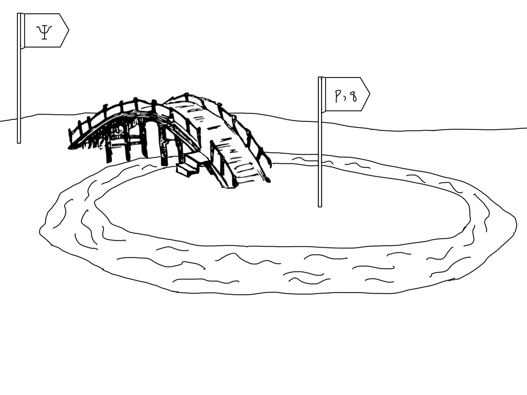
Figure 1: A representation of the ‘bridge’ connecting ‘quantum-land’ with ‘classical-land’.

4 Classical and Quantum Stories for
Additional Quantization Processes

In the analysis in several previous sections we relied heavily on coherent states. To analyze the major tasks in this section it is helpful to initially find suitable coherent states. These coherent states rely on seeking suitable basic quantum operators.

4.0.1 Spin coherent states

For our spin quantization story we will involve three operators, namely $S_{1},S_{2}$, and $S_{3}$, where $[S_{1},S_{2}]=i\hbar\,S_{3}$, as well as cyclic rotations of the operators. The spin coherent states, for $SU(2)$ and $SO(3)$, are chosen as

$$|\theta,\varphi\rangle\equiv e^{-i\varphi S_{3}/\hbar}e^{-i\theta S_{2}/\hbar}\,|s,s\rangle\;,$$ (16)

where $-\pi<\varphi\leq\pi$ and $-\pi/2\leq\theta\leq\pi/2$, and the normalized fiducial vector, $|s,s\rangle$, has the highest eigenvalue for $S_{3}|s,m\rangle=m\hbar|s,m\rangle$, where $m\in\{-s,...,s-1,s\}$, and $S_{1}^{2}+S_{2}^{2}+S_{3}^{2}=\hbar^{2}\,s(s+1)1\!\!1_{s}$. Here $s\in\textstyle{\frac{1}{2}}\{1,2,3,4,...\}$, and the resolution of the identity [7] is given by

$$1\!\!1_{s}=\int|\theta,\varphi\rangle\langle\theta,\varphi|(2s+1)\sin(\theta)\,d\theta\,d\varphi/4\pi\;.$$ (17)

4.0.2 Affine coherent states

For our affine quantization story we will involve two operators, namely $Q$ and $D$, where $0<Q<\infty$ and $[Q,D]=i\hbar\,Q$. Since $Q>0$ the operator $P$ cannot be self adjoint and it is replaced by $D=(PQ+QP)/2$, and both $Q$ and $D$ can be self adjoint. The coherent state parameters are $-\infty<p<\infty$ and $0<q<\infty$, and, for simplicity, we choose $q$ and $Q$ to be dimensionless; hence $p$, $D$, and $\beta$, below, have the dimensions of $\hbar$. The affine coherent states are chosen as

$$|p;q\rangle\equiv e^{ipQ/\hbar}e^{-i\ln(q)D/\hbar}\,|\beta\rangle\;.$$ (18)

In this case, the normalized fiducial vector is chosen as $|\beta\rangle$, where $[(Q-1)+iD/\beta]|\beta\rangle=0$, which implies that $\langle\beta|Q|\beta\rangle=1$ and $\langle\beta|D|\beta\rangle=0$. In this case, the resolution of the identity [7] is given by

$$1\!\!1=\int|p;q\rangle\langle p;q|\,\{[1-\hbar/2\beta]/2\pi\}\;dp\,dq/\hbar\;,$$ (19)

provided $\beta>\hbar/2$.

4.1 Additional quantum to classical and
classical to quantum stories

4.1.1 The spin story

The classical spin Hamiltonian is $G(\theta,\varphi)$ and the classical spin action functional is given by

$$A_{c}={\textstyle\int}_{0}^{T}\{s\hbar\,\cos(\theta(t))\,\dot{\varphi}(t)-G(\theta(t),\varphi(t))\}\;dt\;.$$ (20)

Using the facts that $\langle s,s|S_{3}|s,s\rangle=s\hbar$ and $\langle s,s|S_{1}|s,s\rangle=\langle s,s|S_{2}|s,s\rangle=0$, the affine spin semi-classical action functional is given by

$$A_{sc}={\textstyle\int}_{0}^{T}\{\langle\theta(t),\varphi(t)|[i\hbar(\partial/\partial t)-{\cal{G}}(S_{1},S_{2},S_{3})]|\theta(t),\varphi(t)\rangle\;dt$$

$$\hskip 17.70006pt={\textstyle\int}_{0}^{T}\{\langle s,s|[\cos(\theta(t))\,\dot{\varphi}(t)S_{3}+\dot{\theta}(t)S_{2}$$

$$\hskip 40.00006pt-{\cal{G}}(\cos(\varphi(t))\cos(\theta(t))S_{1}+\cos(\varphi(t))\sin(\theta(t))S_{3}-\sin(\theta(t))S_{2},$$

$$\hskip 40.00006pt\cos(\varphi(t))S_{2}-\sin(\varphi(t))\cos(\theta(t))S_{1}+\sin(\varphi(t))\sin(\theta(t))S_{3},$$

$$\hskip 40.00006pt\cos(\theta(t))S_{3}-\sin(\theta(t))S_{1})]|s,s\rangle\}\;dt$$

$$\hskip 17.8pt={\textstyle\int}_{0}^{T}\{s\hbar\,\cos(\theta(t))\,\dot{\varphi}(t)-G(\theta(t),\varphi(t))\}\;dt\;.$$ (21)

The passage from semi-classical spin functional and twice applying the two pieces of the identity, and then reuniting the two separate parts together, as was done for the canonical story, leads to the quantum affine functional.

4.1.2 The affine story

The classical affine Hamiltonian is $H^{\prime}(pq,q)$, where $0<q<\infty$ and $-\infty<pq<\infty$, and the classical affine action functional is given by

$$A_{c}={\textstyle\int}_{0}^{T}\{-\dot{p}(t)q(t)-H^{\prime}(p(t)q(t),q(t))\}\;dt\;.$$ (22)

The quantum affine Hamiltonian is given by ${\cal H}^{\prime}(D,Q)$, where $Q>0$ and the dilation operator $D=(PQ+QP)/2$. The quantum action functional is given by

$$A_{q}={\textstyle\int}_{0}^{T}\langle\Phi(t)|[i\hbar(\partial/\partial t)-{\cal H}^{\prime}(D,Q)]|\Phi(t)\rangle\;dt\;.$$ (23)

Finally, the semi-classical affine action functional is given by

$$A_{sc}={\textstyle\int}_{0}^{T}\langle p(t);q(t)|[i\hbar(\partial/\partial t)-{\cal H}^{\prime}(D,Q)]|p(t);q(t)\rangle\;dt$$

$$\hskip 18.00005pt={\textstyle\int}_{0}^{T}\langle\beta|[-\dot{p}(t)\,q(t)Q+\dot{q}(t)D/q(t)-{\cal H}^{\prime}(D+p(t)q(t)Q,q(t)Q)]|\beta\rangle\;dt$$

$$\hskip 18.00005pt={\textstyle\int}_{0}^{T}\{-\dot{p}(t)q(t)-H^{\prime}(p(t)q(t),q(t))\}\;dt\;,$$ (24)

thanks to the facts that $\langle\beta|Q|\beta\rangle=1$ and $\langle\beta|D|\beta\rangle=0$.

The passage from semi-classical affine functional and twice applying the two pieces of the identity, and then reuniting the two separate parts together, as was done for the canonical story, leads to the quantum affine functional.

L. Gouba has examined an affine quantization of a free particle and an half-harmonic oscillator, where both problems require that $0<q<\infty$, and was able to extract the eigenfunctions and eigenvalues for the half-oscillator problem [8]. While the eigenfunctions are quite different, the eigenvalues for this example are equivalent to those of a full-harmonic oscillator in that they are equally spaced. This puts these results within the larger set of harmonic oscillator type problems.

4.2 Additional examples of a smooth and combined
quantum and classical story

The article [9] summarizes the author’s approach to non-renormalizable covariant scalar fields as well as his approach to quantum gravity. While a canonical quantization approach to these problems has faced difficulties, an affine quantization has come through with flying colors. Readers of the present paper may have noticed that an affine approach is very similar to a canonical approach to quantization, the only difference between the two procedures is that (favored) canonical variables, such as $p$ and $q$, are promoted to quantum operators, while (favored) affine variables, such as $pq$ and $q$, are promoted to quantum operators. In [10], the reader would find a natural analysis that this choice of basic affine variables to promote to quantum operators makes good sense.

Affine procedures that are applied to the difficult problems being considered here, already have equations, such as their Schrödinger equations, which are ready for approximate $-$ or perhaps even exact $-$ solutions to be found. Hopefully, smooth procedures between classical and quantum systems may play a helpful role in further analysis.

References

• [1] See, for example, E. SchrΓΆdinger, β€œAn Undulatory Theory of the Mechanics of Atoms and Molecules”, Physical Review 28 6, 1049-1070 (1926); DOI:10.1103/PhysRev28,1049.
• [2] P.A.M. Dirac, The Principles of Quantum Mechanics, (Claredon Press, Oxford, 1958), page 114, in a footnote.
• [3] J.R. Klauder, β€œQuantum Gravity Made Esay”, JHEPGC 6, 90-102 (2020); arXiv:1903.11211; DOI:10.4326/jhepgc.20206.61009.
• [4] http://en.wikipedia.org/wiki/ Fubini-Study_metric.
• [5] J.R. Klauder, β€œThe Favored Classical Variables to Promote to Quantum Operators”; arXiv:2006.13283.
• [6] G.Y.H. Avossevon, J.V. Hounguevou, D.S. Takay, β€œConventional and Enhanced Canonical Quantization, Application to Some Simple Maniflods”, Journal of Modern Physics 4, 1476-1485 (2013); DOI:10.4236/jmp.2013.41117.
• [7] J.R. Klauder, A Modern Approach to Functional Integration, (BirkhΓ€user, New York, 2011); DOI:10.1007/978-0-8176-4791-9.
• [8] L. Gouba, β€œAffine Quantization on the Half Line”; arXiv:2005.08696.
• [9] J.R. Klauder, β€œUsing Affine Quantization to Analyze Non-renormalizable Scalar Fields and the Quantization of Einstein’s Gravity”; arXiv:2006.09156.
• [10] J.R. Klauder, β€œThe Benefits of Affine Quantization”, JHEPGC 6, 175-185 (2020); arXiv:1912.08047; DOI:10.4236/jhepgc.2020.62014.