Test-Cost Sensitive Methods for Identifying Nearby Points

Abstract

Real-world applications that involve missing values are often constrained by the cost to obtain data. Test-cost sensitive, or costly feature, methods additionally consider the cost of acquiring features. Such methods have been extensively studied in the problem of classification. In this paper, we study a related problem of test-cost sensitive methods to identify nearby points from a large set, given a new point with some unknown feature values. We present two models, one based on a tree and another based on Deep Reinforcement Learning. In our simulations, we show that the models outperform random agents on a set of five real-world data sets.

Introduction

In many real-world setting, resources, such as money, energy, time, limit the amount of information one can ascertain. Medical practitioners focus on arriving at a diagnosis as quickly and cost efficiently as possible. Survey makers aim to design a small yet revealing set of questions. Pilots require making split-second decisions by using a limited set of measurements from a multitude of sensors, among many other examples. In all these cases, there are two forces at play: on one hand, the agent tries to minimize the total cost of the features it gathers, while simultaneously optimizing its ability to make the correct decision. When applied to classification, this gives rise to the Classification with Costly Features (CwCF) (or Test-Cost Sensitive Classification) problem, which has been extensively studied by many researchers.

In this setting, an algorithm classifies an instance using only the features it chose to reveal at defined costs. For each instance, the algorithm sequentially selects the next feature to obtain conditioned on the currently available information. This sets test-cost sensitive methods apart from feature selection/pruning: the set of features to reveal is inherently local to the instance. Keeping the same setting of costly features, this paper tackles a simple yet surprisingly difficult problem:

Problem 1

Given a complete data set (where values for all features are known) $D$, an instance $p$ with some unknown feature values drawn from the same distribution, and a budget $B$, find the optimal set of features to reveal with total cost $\leq B$ such that instances in $D$ closest to the completed $p$ (in distance) can be identified.

In healthcare, this could help find similar patients for prognostic purposes, while in recommender systems, this could assist in early detection of similar users. This problem is also closely linked to a data repair problem of data imputation since knowing the most similar and dissimilar points can be used to complete the missing features. Human-in-the-loop feature revealing methods (without consideration for feature costs) have been successfully applied to data repair systems, such as the Guide Data Repair (GDR) system of (Yakout et al. 2011).

The difficulty of this problem comes from the fact we are attempting to measure distance using a lossy embedding. For example, given two complete points $c_{1}=(1,0)$, $c_{2}=(2,2)$, and an incomplete point $p=(1,?)$, there is no way of knowing whether $p$ is closer to $c_{1}$ or $c_{2}$ if the distribution of the $y$-coordinate is random. However, if $\Pr(p.y<5/4|x=1)>\Pr(p.y\geq 5/4|x=1)$, then it is more probable that $p$ is closer to $c_{1}$. Furthermore, if $p.y$ is functionally dependent on $p.x$, simply knowing $p.x$ would be enough to compute the distance. In this view, Problem 1 can be restated as finding the optimal set of features such that projecting $D$ to a feature space with only the known features preserves the relative distances from $p$ to the points of $D$ well. While such optimal sets may not exist for random distributions, we will show that this often holds for many real-life data sets.

Test-cost sensitive learning can be cast as a Markov Decision Process (MDP) (Zubek, Dietterich et al. 2004), and test-cost sensitive algorithms typically fall into two categories: inductive, often tree-based, learning (Turney 2002; Chai et al. 2004; Maliah and Shani 2018) and reinforcement learning (Dulac-Arnold et al. 2011; Janisch, Pevnỳ, and Lisỳ 2019). While Janisch, Pevnỳ, and Lisỳ (2019) shows that Deep Q-learning outperforms problem specific inductive learning models, explainability is desired in many domains. Following these previous works, we present two models: a subspace clustering model based on the CLusterTree (CLTree) model (Liu, Xia, and Yu 2005) and a Deep Q-learning model. We evaluate these models using public data sets against random agents and show that both models outperform random agents. We are not aware of any work solving the same problem that we can benchmark against.

Problem formulation

We begin by discussing how to describe a solution to Problem 1. While the obvious choice is to compute something akin to the $k$ nearest neighbours of an instance $p$, this creates a large output space which makes learning harder. Instead, we take a more generalizable approach and return nearby clusters after partitioning $D$ using a distance-based clustering algorithm. Furthermore, if the notion of membership for an arbitrary points exists (as is the case of $k$-means and CLTree), we can return $p$’s most probable cluster. This provides a succinct output that still allows users to retrieve similar points in $D$.

Given clusters $C_{1},\dots,C_{m}$ of $D$ and an instance $p$ with only features $\bar{\mathcal{F}}\subseteq\mathcal{F}=\{f_{1},\dots,f_{n}\}$ known, we need to measure how well $\bar{\mathcal{F}}$ preserves relative distances. Let $\mathfrak{R}_{\bar{\mathcal{F}},i}(p)$ be a prediction of the ranking of $C_{i}$ and $\mathfrak{R}_{\mathcal{F},i}(p)$ be its true ranking, such that $C_{i}$ with rank $1$ contains elements that are most similar to $p$ and rank $n$ most dissimilar (for some measure of similarity). We define the score function $S(\bar{\mathcal{F}},p)$ as the mean squared error (MSE) of the rankings:

$$S(\bar{\mathcal{F}},p)=\frac{1}{m}\sum_{i}(\mathfrak{R}_{\bar{\mathcal{F}},i}(p)-\mathfrak{R}_{\mathcal{F},i}(p))^{2}.$$ (1)

When $S(\bar{\mathcal{F}},p)=0$, it means that measuring the similarity between $p$ and each cluster is no different if we use $\bar{\mathcal{F}}$ or all the features $\mathcal{F}$. Let $c:\mathcal{F}\mapsto\mathbb{R}$ the cost function mapping feature $f_{i}$ to some real-valued normalized cost (that is, $1\geq c(f)\geq 0$ for all features). Finally, we want to find parameters $\theta$ for function $z_{\theta}(p)=\bar{\mathcal{F}}_{p}$ that minimizes the expected sum of MSE and (scaled) total cost:

$$\operatorname*{arg\,min}_{\theta}\frac{1}{|D|}\sum_{p_{j}\in D}\left(\left(\sum_{f\in\bar{\mathcal{F}}_{p_{j}}}\alpha c(f)\right)+S(\bar{\mathcal{F}}_{p_{j}},p_{j})\right)$$ (2)

To formulate Problem 1 as a MDP, let $(x_{1},\dots,x_{n})\in D$ be a point in $D$, where $0\leq x_{i}\leq 1$ is a normalized value of feature $f_{i}\in\mathcal{F}$. Let $B\in\mathbb{R}$, called the budget, be the maximum allowed cost incurred by the agent. We define the state space as

$$\mathcal{S}=\{((x_{1},\dots,x_{n}),\bar{\mathcal{F}},\bar{c})\},$$

where $\bar{\mathcal{F}}\subseteq\mathcal{F}$ is the current set of selected features and $\bar{c}=\sum_{f_{i}\in\bar{\mathcal{F}}}c(f_{i})$ is the current cost. A state $s\in\mathcal{S}$ is terminal if there exist no feature $f_{j}\notin\bar{\mathcal{F}}$ such that $\sum_{f_{i}\in\bar{\mathcal{F}}}c(f_{i})+c(f_{j})\leq B$.

The set of available actions is $\mathcal{A}=\mathcal{A}_{f}\cup\{\mathcal{A}_{t}\}$, where $\mathcal{A}_{f}=\{f_{1},\cdots,f_{n}\}$ reveals feature $f_{i}$ and $\mathcal{A}_{t}$ terminates the episode. The reward function $r:\mathcal{S}\times\mathcal{A}\mapsto\mathbb{R}$ is

$$r(s,a)=\begin{cases}-\alpha c(a)&\text{if $a\in\mathcal{A}_{f}$}\\ -S(\bar{\mathcal{F}},p)&\text{if $a=\mathcal{A}_{t}$}\end{cases}$$

The parameter $\alpha$ balances the cost with the score: higher values of $\alpha$ will make the agent favour lower cost episodes and vice versa. Starting from initial state $s_{0,p}=(p,\phi,0),p\in D$ (where no features are known), let $s_{t,p}=(p,\bar{\mathcal{F}}_{p},\bar{c}_{p})$ be the terminal state following the optimal policy $\pi_{\theta}$ that maximizes the sum of rewards for this episode:

$$\sum_{a_{i}}r(s_{i},a_{i})=-\alpha\bar{c}_{p}-S(\bar{\mathcal{F}}_{p},p).$$

The expected sum of rewards over all $p\in D$ is

$$\frac{1}{|D|}\sum_{p}(-\alpha\bar{c}_{p}-S(\bar{\mathcal{F}}_{p},p)).$$

This is maximized when equation 2 is minimized for fixed budget $B$; thus, finding the optimal policy to the MDP solves Problem 1.

Inductive learning

The CLTree model of (Liu, Xia, and Yu 2005) uses a technique called subspace clustering, which was developed to effectively cluster high-dimensional data. Subspace clustering algorithms project different partitions of the data to different subspaces and find clusters within those selected subspaces. This allows the algorithm to judge if features are important locally, conditioned on being in some subspace; thus, this is a very natural framework to solve Problem 1. For a survey of this topic, we direct the readers to (Parsons, Haque, and Liu 2004).

In this section, we present a novel subspace clustering model, named Cost Balancing Clustering Tree (CBCTree), which can be see as an extension of the CLTree model that accounts for costly features. In order to facilitate this, we have to use a different measure of gain than the CLTree. Furthermore, we must also define cluster membership with unknown values.

The basic outline of the algorithm follows the well known ID3 algorithm (Quinlan 1986): at each iteration, we choose the (locally) optimal feature/value and recursively partition the data until some stopping criteria. For this, we must first quantify a ‘good’ split. Given a set of points $D$, let $c_{D}$ be its centroid and $\delta_{D}$ be the average distance between $c_{D}$ and all points in $D$. Define a boundary $b$ to be a pair $(f,v)$, where $f$ is a feature and $v$ its value, and the left partition induced by $b$ on $D$ as:

$$D_{(b,l)}=\{p|p\in D,p.f<v\}.$$

The right partition is $D_{(b,r)}=D\setminus D_{(b,l)}$. A boundary $b$ is a good split if the partitions induced have smaller expected average distances to their respective centroids (see Figure 1).

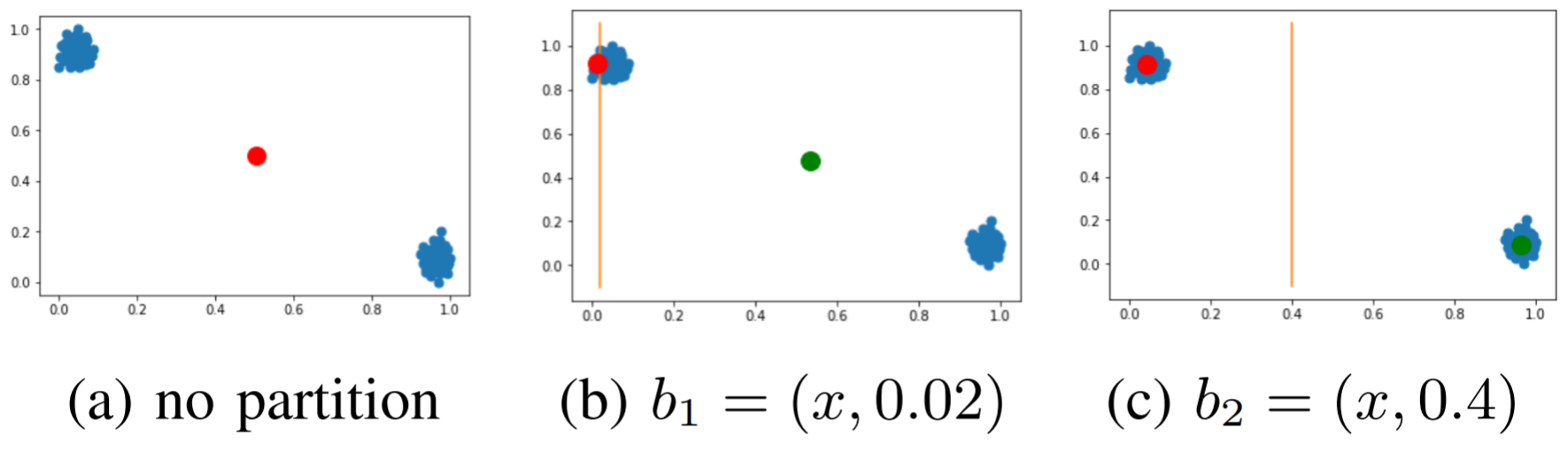
Figure 1: Examples of partitions. While $b_{1}$ makes the average distance to the left centroid small, the average distance to the right centroid is large; $b_{2}$ is more balanced.

Formally, we define the score of splitting at boundary $b$ as:

$$S(D,b)=p_{l}(\delta_{D}-\delta_{D_{(b,l)}})+p_{r}(\delta_{D}-\delta_{D_{(b,r)}}),$$

where $p_{*}=|D_{(b,*)}|/|D|$. Since $p_{l}+p_{r}=1$, we can simplify the above as $S(D,b)=\delta_{D}-(p_{l}\delta_{D_{(b,l)}}+p_{r}\delta_{D_{(b,r)}}))$. Finally, we define the reward as the score discounted by the (scaled) cost of obtaining that feature:

$$R(D,b)=(1-\alpha c(b.f))S(D,b).$$

At each node $N$, we enumerate the features and evenly spaced values from the domain of each feature. We then find the feature/value pair $b$ that maximizes $R(D_{N},b)$. We stop when the number of points is less than $\tau$, although other stopping criteria are possible. In terms of the complexity, we examine $|D_{N}|$ elements at most $|\mathcal{F}|\cdot\ell$ times, where $\ell$ is the number of evenly spaced values. For a tree of height $h$, this gives an upper bound of $O(|D||\mathcal{F}|\ell h)$ for construction.

Algorithm 1 build_CBCT($D$)

Input: $D$ - dataset
Output: $T$ - resulting tree

1. if $|D|\leq\tau$: return $T=(D,-,-)$

2. for $f\in\mathcal{F}\setminus\bar{\mathcal{F}}$:

   1. $\ell=\text{linspace}(f_{min},f_{max})$

   2. for $v\in\ell$:

      1. $b_{(f,v)}:=(f,v)$

      2. compute $R(D,b_{(f,v)})$

3. $b_{max}=\text{arg max}_{b}S(D,b)$

4. set $c(b_{max}.f):=0$

5. $T_{l}:=\text{build\_CBCT}(D_{(b_{max},l)})$

6. $T_{r}:=\text{build\_CBCT}(D_{(b_{max},r)})$

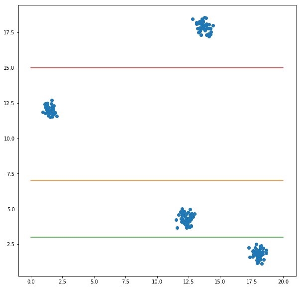
(a) points and boundaries

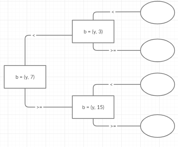
(b) translated tree

Figure 2: Example of a CBCTree produced by a simple data set at uniform cost for each feature $x,y$. The rectangles denote decision nodes while the ovals are terminal nodes. Note the order of the splits; the first split divides the data in half, rather than singling out one cluster. Also, the $x$-values are never used as a boundary; while there are conflicts in the $x$-value between clusters, each subspace created does not have any conflicts.

Suggested action and cluster prediction

Given a set of $\bar{\mathcal{F}}$ strict subset of $\mathcal{F}$, we want to use a CBCTree $T$, as constructed by the algorithm build_CBCT, to suggest the next action to take. Since the features that decreases the average distance the most are closer to the root of the tree, we can traverse down the tree using features in $\bar{\mathcal{F}}$ and stop at the first node using a feature $f\notin\bar{\mathcal{F}}$ as the boundary. Define $\mathcal{N}_{\bar{\mathcal{F}},f,p}$ as the set of nodes reachable with features $\bar{\mathcal{F}}\cup\{f\}$ following these rules of traversal at each node: 1) if the splitting feature is known, go down the appropriate branch; 2) if the splitting feature is $f$, go down both branches; 3) otherwise, add the node to $\mathcal{N}_{\bar{\mathcal{F}},f,p}$. For each node $N\in\mathcal{N}_{\bar{\mathcal{F}},f,p}$, the similarity score of point $p$ with features $\bar{\mathcal{F}}$ is:

$$\mathfrak{S}(N,p,\bar{\mathcal{F}})=\left(\frac{|D_{N}|}{|D_{\text{total}}|}\sum_{p^{\prime}\in D_{N}}\sqrt{\sum_{f_{i}\in\bar{\mathcal{F}}}(p.f_{i}-p^{\prime}.f_{i})^{2}}\right)^{-1},$$

where $|D_{\text{total}}|=\sum_{N\in\mathcal{N}_{\bar{\mathcal{F}},f,p}}|D_{N}|$ is the number of total data points in $N_{\bar{\mathcal{F}},f,p}$. The value $\mathfrak{S}$ is the reciprocal of the average L2 distance between each point of $D_{N}$ and $p$, only using features $\bar{\mathcal{F}}$. Let $C_{N}$ be the cluster defined by node $N$ (that is, the region defined by the boundaries to reach $N$), then $\mathfrak{S}(N,p,\bar{\mathcal{F}})$ is a measure of how well $p$ ‘fits’ into this cluster. Approximating the probability of $p$ was chosen from $C_{N}$ as $\frac{|D_{N}|}{|D_{\text{total}}|}$, $\sum_{N\in\mathcal{N}_{\bar{\mathcal{F}},f}}\mathfrak{S}(N,p,\bar{\mathcal{F}})$ is the expected similarity score for revealing $f$ given we have $\bar{\mathcal{F}}$. The higher this score, the more confident the model is that revealing $f$ is useful. Similarly, let $\mathcal{N}_{\bar{\mathcal{F}},p}$ be the set of nodes reachable by the same rules above, but splitting on every feature $f\in(\mathcal{F}\setminus\bar{\mathcal{F}})$. This represents the set of all clusters that $p$ could belong to. For each $N\in\mathcal{N}_{\bar{\mathcal{F}},p}$, we compute $\mathfrak{S}(N,p,\bar{\mathcal{F}})$ and classify $p$ into $C_{N}$ that maximizes this value (see algorithms 2 and 3).

Algorithm 2 compute_$\mathcal{N}_{\bar{\mathcal{F}},f}(T,p)$

Input: $T$ - tree; $p$ - point
Output: $\mathcal{N}_{f}$

1. if $T$ is empty: return $\{\}$

2. if $T$ is a leaf: return $\{T.\text{node}\}$

3. set $b$ to be the boundary at current node

4. if $p[b.f]$ is known:

   1. if $p[b.f]>b.v$: return compute_$\mathcal{N}_{\bar{\mathcal{F}},f}(T.\text{right},p)$

   2. else: return compute_$\mathcal{N}_{\bar{\mathcal{F}},f}(T.\text{left},p)$

5. else if $b.f=f$:

   1. $\mathcal{N}_{\bar{\mathcal{F}},f}^{(r)}=\text{compute\_}\mathcal{N}_{\bar{\mathcal{F}},f}(T.\text{right},p)$

   2. $\mathcal{N}_{\bar{\mathcal{F}},f}^{(l)}=\text{compute\_}\mathcal{N}_{\bar{\mathcal{F}},f}(T.\text{left},p)$

   3. return $\mathcal{N}_{\bar{\mathcal{F}},f}^{(r)}\cup\mathcal{N}_{\bar{\mathcal{F}},f}^{(l)}$

6. else: return $\{T.\text{node}\}$

Algorithm 3 compute_$\mathcal{N_{\bar{\mathcal{F}}}}(T,p)$

Input: $T$ - tree; t - tuple
Output: $\mathcal{N}$

1. if $T$ is empty: return $\{\}$

2. if $T$ is a leaf: return $\{T.\text{node}\}$

3. let $b$ be the boundary at current node

4. if $t[b.f]$ is known:

   1. if $t[b.f]>b.v$: return compute_$\mathcal{N_{\bar{\mathcal{F}}}}(T.\text{right},p)$

   2. else: return compute_$\mathcal{N_{\bar{\mathcal{F}}}}(T.\text{left},p)$

5. else:

   1. $\mathcal{N}^{(r)}=$ compute_$\mathcal{N_{\bar{\mathcal{F}}}}(T.\text{right},p)$

   2. $\mathcal{N}^{(l)}=$ compute_$\mathcal{N_{\bar{\mathcal{F}}}}(T.\text{left},p)$

   3. return $\mathcal{N_{\bar{\mathcal{F}}}}^{(r)}\cup\mathcal{N_{\bar{\mathcal{F}}}}^{(l)}$

Policy learning

To solve MDP problems we estimate the optimal values of taking an action $a$ on state $s$. Q values are shaped by the expected future sum of rewards when taking $a$ on $s$ and then following the optimal policy thereafter. An optimal policy can be derived by greedily selecting the actions with the highest values at each state which satisfies the Bellman equation:

$$Q^{*}(s,a)=\operatorname{\mathbb{E}}_{s^{\prime}}\left[R+\gamma\max_{a^{\prime}}Q^{*}(s^{\prime},a^{\prime}|s,a)\right]$$

We train a Deep Q Network (DQN) to schedule features that maximizes the ranking of the clusters while lowering cost incurred by the agent.

Deep Q-learning

Deep Q-learning introduces a target network, with parameters $\psi$, which follows an online network, with parameters $\theta$ (Mnih et al. 2015). The target network copies the parameters $\theta$ of the online network every $\tau$ steps, and for every other step, $\psi$ is fixed. The target used by the DQN is:

$$Y^{Q}_{t}=R_{t+1}+\gamma\max_{a\in\mathcal{A}}Q_{\psi}(s_{t+1},a)$$

where $\gamma$ is a scalar step size and $\mathcal{A}$ is the set of available actions to take at state $s$. To optimize the agent, we minimize the Bellman mean squared error $\ell$ for a batch of transitions:

$$\ell_{\theta}=\operatorname{\mathbb{E}}\left[\left(Y_{t}^{Q}-Q_{\theta}(s_{t},a_{t})\right)^{2}\right]$$

Double Deep Q Networks

In Q-learning and DQN, using the $\max$ operator to select and evaluate actions leads to over-optimistic value estimates (Van Hasselt 2010). Double DQN is a technique which reduces this bias by rewriting the Q-value equation with respect to both online network $Q_{\theta}$ and target network $Q_{\psi}$ (Van Hasselt, Guez, and Silver 2016). They define the target $Y^{Q}_{t}$ as:

$$Y^{Q}_{t}=R_{t+1}+\gamma Q_{\psi}(s_{t+1},\operatorname*{arg\,max}_{a\in\mathcal{A}}Q_{\theta}(s_{t+1},a))$$

Dueling Deep Q Networks

Dueling DQN stabilizes and accelerates training by decomposing the Q-value function into value and advantage functions (Wang et al. 2016). The network outputs an estimate of the value stream $V_{\theta}$ and advantage stream $A_{\theta}$ to construct the Q-value function as:

$$Q_{\theta}(s,a)=V_{\theta}(s)+\left(A_{\theta}(s,a)-\frac{\sum_{a^{\prime}}A_{\theta}(s,a^{\prime})}{|\mathcal{A}|}\right)$$

State

In the DQN case, we follow a similar definition to $\mathcal{S}$ as defined in the Problem Formulation section. Since each state $s_{t,p}$ is composed of point $p$, learning Q-values over the states in $\mathcal{S}$ is a difficult task for this problem; small perturbations in the values of $p$ can change the order of the rankings. To reduce the state space of $\mathcal{S}$, for each state $s_{t,p}=(p,\bar{\mathcal{F}}_{p},\bar{c}_{p})$, we substitute $p$ with a multi-hot encoding $e_{t}$ to denote the features which are known at time step $t$.

Action selection

Recall that each action in $\mathcal{A}_{f}$ is a request for feature and the episode terminates when the agent chooses the action $\mathcal{A}_{t}$. To restrict the DQN to perform only actions in $\mathcal{A}_{f}$, we define the mask $m_{t}$ to be $m_{t}=(\mathbf{1}-e_{t})$ where $\mathbf{1}$ is a vector of all ones. Additionally, $1$ is appended to $m_{t}$ to resemble the action $\mathcal{A}_{t}$. We redefine the target function to include only available actions $\mathcal{A}$ by applying the mask:

$$Y^{Q_{\mathcal{A}}}_{t}=Y^{Q}_{t}\odot m_{t}$$

Algorithm 4 step(s,a)

Input: $s=(p,\bar{\mathcal{F}},\bar{c})$ - state; $a\in\mathcal{A}$ - action
Output: $s^{\prime}$ - next state; $r$ reward

1. if $a=\mathcal{A}_{t}$:

   1. $r=-S(\bar{\mathcal{F}},p)$

2. else:

   1. $r=-\alpha c(a)$

   2. $s^{\prime}=(p,\bar{\mathcal{F}}\cup\{a\},\bar{c}+c(a))$

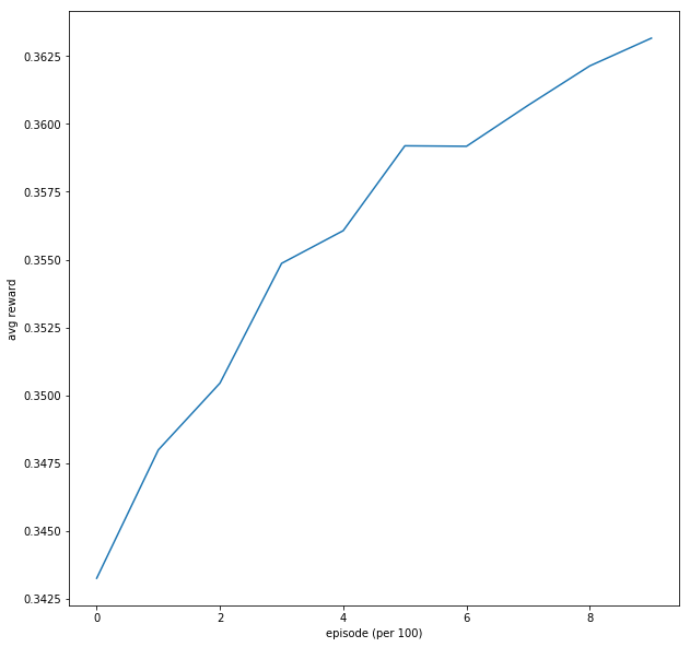
Figure 3: Plot of the average reward per 100 episodes during training for DQN using the data set heartfail.

Reward

To calculate the reward $r(s,a)$ received upon performing $\mathcal{A}_{t}$ (See Algorithm 4), we compute $S(\bar{\mathcal{F}},p)$ as defined in Equation 1. Concretely, the score function in Equation 1 is dependent on the implementation of the true ranking $\mathfrak{R}_{\mathcal{F},i}(p)$ and predicted ranking $\mathfrak{R}_{\bar{\mathcal{F}},i}(p)$ functions. Let

$$d(p,p^{\prime},\bar{\mathcal{F}})=\sqrt{\sum_{f\in\bar{\mathcal{F}}}(p^{\prime}.f-p.f)^{2}}$$

be the distance between $p$ and $p^{\prime}$, using only $\bar{\mathcal{F}}$. To derive the true ranking $\mathfrak{R}_{\mathcal{F},i}(p)$, we first cluster $D$ via K-means, producing cluster centroids $C_{1},\dots,C_{m}$. We then order each cluster by $d(p,C_{i},\mathcal{F})$, defining this order as the true rank $\mathfrak{R}_{\mathcal{F},i}$. Similarly, given some $\bar{\mathcal{F}}$, we order each cluster by $d(p,C_{i},\bar{\mathcal{F}})$, defining this order as the predicted rank $\mathfrak{R}_{\bar{\mathcal{F}},i}(p)$. Other implementations of clustering/ranking is possible; for instance, we could use the Gaussian mixture model and rank the clusters by likelihood of observing $p$ given the distribution of a cluster.

Comparison to inductive learning

While both the CBCTree and DQN model aims to solve Problem 1, there are several differences between the two models. First, the CBCTree both clusters the data and provides a schedule of feature updates, whereas our DQN model requires the clusters to be provided externally. Consequentially, the results of CBCTree are more interpretable as the boundaries of the clusters are explicitly computed. On the other hand, the ‘black box’ approach of the DQN model is more flexible since the external clustering algorithm is exchangeable. Second, the CBCTree learns a hypothesis that is point (datum) wise, while our DQN model uses binary features. We discuss the experimental implications in the next section.

The two models also differ in behavior when the features revealed are not following the model’s learned policy. The suggested next feature update is fixed for the CBCTree to be the first unknown feature encountered when traversing the tree. Any other revealed feature is used to compute the similarity score $\mathfrak{S}$. In Q-learning, the Q-value function is defined for all possible states; thus, the model can dynamically suggest the next update regardless of whether the users follow the learned policy.

Analysis

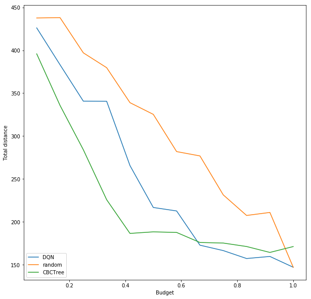
(a) heartfail

(b) breastcancer

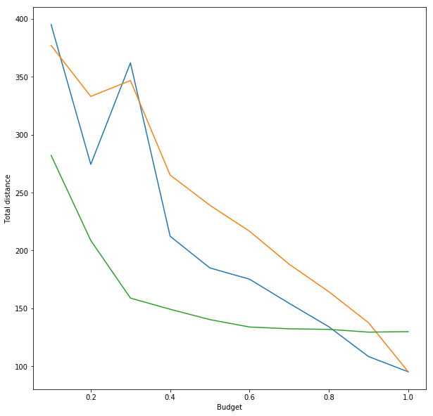
(c) liver

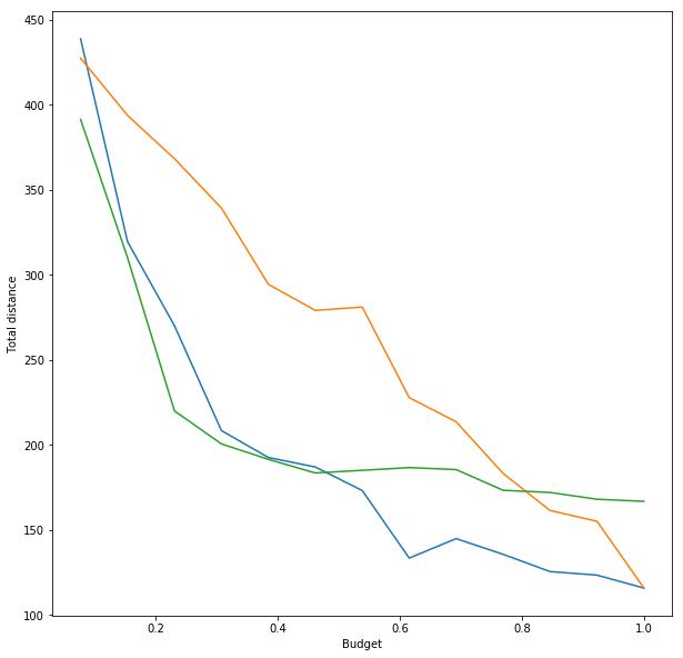
(d) hcv

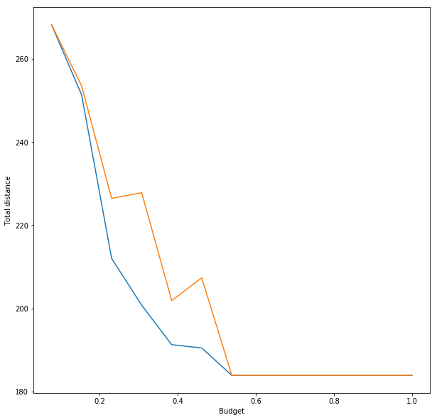
(e) heart

Figure 4: Comparison of CBCTree, DQN, and random models

We compare the performance of CBCTree, DQN, and an agent that takes random actions at equal probability over all possible remaining actions at each step. The first goal is to measure whether or not we can perform better than selecting random features to reveal in real-life data sets. The second goal is to measure which model performs the best; in particular, whether point-wise policies outperform feature-wise policies.

Environment Setup

We use several publicly available data sets (Dua and Graff 2017), which are summarized in Table 1. For each set, we normalize data with its mean and range then divide the data into training $D_{tr}$ and test $D_{t}$ sets. Other than ‘heart’, all costs are set uniformly to be $1/m$, where $m$ is the number of features. For heart, we use the provided costs from Ontario Health Insurance Plan (OHIP)’s fee schedule. Furthermore, we used the provided ‘groups’, which are sets of attributes such that revealing one feature in a group will reveal the rest of the features in that group essentially at no additional cost. For this, we omit the CBCTree as we have not yet implemented this feature yet, although such scheduling is extremely natural for reinforcement learning.

Name	feat	#train	#test
heart	13	243	60
breastcancer	9	547	136
hcv	13	493	122
heartfail	12	240	59
liver	10	464	115

Table 1: Summary of data sets

We use the training set to construct each model at some fixed budget. While some hyper-parameter tuning was performed to ensure that the models converged, we did not do extensive tuning. The same hyper-parameters are used for each data set. We also found that smaller DQN networks performed similarly to larger networks. For each instance $p$ in the test set, we start at the initial state $(p,\phi,0)$ and apply the learned policies, providing the feature value as needed. For the DQN and random agent, we first cluster the training set into $K$ clusters using scikit-learn (Buitinck et al. 2013).

Recall that

$$d(p,p^{\prime},\bar{\mathcal{F}})=\sqrt{\sum_{f\in\bar{\mathcal{F}}_{p}}(p^{\prime}.f-p.f)^{2}}$$

is the distance between $p$ and $p^{\prime}$ only using the revealed features $\bar{\mathcal{F}}$. For the DQN and random models, after applying the learned policies, we predict $k=5$ closest points in $D_{tr}$ for each $p\in D_{t}$ by finding $k$ points $p_{i}\in D_{tr}$ such that $p_{i}$ has the $i$-th minimal value $d(p,p_{i},\bar{\mathcal{F}})$. Note that when $\bar{\mathcal{F}}_{p}=\mathcal{F}$, this is the $k$ closest points in the training set to $p$. For the CBCTree, we still predict $k$ closest points, but only within the predicted cluster. This is to better preserve the hard boundaries that the CBCTree computes, since cluster dissimilarity is less clear on the CBCTree. Finally, we report $\sum_{i}d(p,p_{i},\mathcal{F})$, the sum of the true distances between $p$ and $p_{i}$’s.

Discussion

Figure 4 shows the results of the three models on the data sets. For each plot, the x-axis shows the allotted budget and the y-axis shows the sum of the $k$ true distances described in the previous section; thus, lower points on the plot are better.

There are several interesting observations we can make from these experiments. Firstly, with the exception of breastcancer, the CBCTree and DQN models outperform the random agent. This is an important result because it confirms that similar or ‘close’ points can be identified without requiring the whole feature set, and additionally holds when the importance of features are non-uniform. This is already a well-established concept in classification (for example, feature selection), but it is not immediately clear that such techniques are applicable when determining similarity. Intuitively, if two entities are known to be similar in some aspect (eg. medical condition), then they should also be similar in relevant features to that aspect, even if other unrelated measures differ (eg. hair colour); our experiments give evidence that this intuition holds.

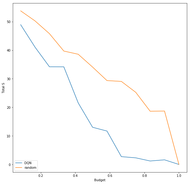
Figure 5: $\sum_{p\in D_{t}}S(\bar{\mathcal{F}},p)$ for heartfail

Secondly, the fact that we are able to retrieve nearby points by optimizing Equation 1 shows that ranking the clusters is a useful proxy to solve Problem 1. Figure 5 shows this in detail by plotting $\sum_{p\in D_{t}}S(\bar{\mathcal{F}},p)$ for DQN and random agents for the data set heartfail. The shapes of both graphs are remarkably similar, which would be the case if they were indeed closely related.

Thirdly, we can see that CBCTrees decrease distances faster at lower costs, but perform worse at higher costs. This is due to the soft/hard boundaries discussed above. In particular, if the data has many points whose membership to a single cluster is ambiguous, then hard boundaries may cause close points to be classified into different clusters. The difference in the type of hypothesis learned could also explain why the CBCTrees perform better at lower costs. Since the DQN model uses binary features and we are always starting from an empty initial state, we are essentially using the Q-value learned by the agent to select features. At lower budgets, selecting features globally is much less flexible than the point-wise method of the CBCTree, but the difference is less pronounced as we increase the budget. One notable case where the DQN model perform even worse than the random agent is breastcancer. The fact the CBCTree performs the best could imply that there exists data sets whose features are equally important globally, but not locally conditioned on being in some subspace.

Future works

In the future, there are several extensions we plan to pursue. Firstly, from an algorithmic perspective, solving Problem 1 allows for us to search for the K nearest neighbours (KNN) when there are missing features. One application of this is to extend the current algorithm to work over time series data (possibly by applying a heavier cost to entries further back in the past as they may be harder to retrieve than more current entries) and apply the KNN classifier algorithm along with dynamic time warping, which has been shown to outperform many more sophisticated models (Ding et al. 2008).

A second direction is to consider how such human-in-the-loop feature updates can interact with completely automatic feature completion models, such as low rank matrix completion. Since we are identifying nearby points, this could, in theory, help algorithms determine some range of possible values. One experiment would be, for instance, to see if following the schedule of updates provided by either the CBCTree or DQN models can improve the performance of a completion algorithm compared to randomly choosing values to supply.

Conclusion

In this paper, we have proposed test-cost sensitive methods to identify similar or ‘close’ points, given a new point with unknown feature values. We introduced two domain-independent methods that utilize our proposed MDP framework to optimize total feature cost and nearby point similarity. In five real-world datasets, both DQN and CBCTree outperform random policies in revealing features that maximize nearby point similarity. Furthermore, we found that Deep Q-learning performs well with only a few parameters in our MDP framework, enabling deployment in real-world settings.

Although there is a growing body of research in test-cost sensitive methods, current efforts are focused on the context of classification. We hope that test-cost sensitive methods for identifying nearby points introduce a motivated and challenging environment for future research.

References

- Buitinck et al. (2013) Buitinck, L.; Louppe, G.; Blondel, M.; Pedregosa, F.; Mueller, A.; Grisel, O.; Niculae, V.; Prettenhofer, P.; Gramfort, A.; Grobler, J.; Layton, R.; VanderPlas, J.; Joly, A.; Holt, B.; and Varoquaux, G. 2013. API design for machine learning software: experiences from the scikit-learn project. In ECML PKDD Workshop: Languages for Data Mining and Machine Learning, 108–122.
- Chai et al. (2004) Chai, X.; Deng, L.; Yang, Q.; and Ling, C. X. 2004. Test-cost sensitive naive bayes classification. In Fourth IEEE International Conference on Data Mining (ICDM’04), 51–58. IEEE.
- Ding et al. (2008) Ding, H.; Trajcevski, G.; Scheuermann, P.; Wang, X.; and Keogh, E. 2008. Querying and Mining of Time Series Data: Experimental Comparison of Representations and Distance Measures. Proc. VLDB Endow. 1(2): 1542–1552. ISSN 2150-8097. doi:10.14778/1454159.1454226. URL https://doi.org/10.14778/1454159.1454226.
- Dua and Graff (2017) Dua, D.; and Graff, C. 2017. UCI Machine Learning Repository. URL http://archive.ics.uci.edu/ml.
- Dulac-Arnold et al. (2011) Dulac-Arnold, G.; Denoyer, L.; Preux, P.; and Gallinari, P. 2011. Datum-wise classification: a sequential approach to sparsity. In Joint European Conference on Machine Learning and Knowledge Discovery in Databases, 375–390. Springer.
- Janisch, Pevnỳ, and Lisỳ (2019) Janisch, J.; Pevnỳ, T.; and Lisỳ, V. 2019. Classification with costly features using deep reinforcement learning. In Proceedings of the AAAI Conference on Artificial Intelligence, volume 33, 3959–3966.
- Liu, Xia, and Yu (2005) Liu, B.; Xia, Y.; and Yu, P. S. 2005. Clustering via decision tree construction. In Foundations and advances in data mining, 97–124. Springer.
- Maliah and Shani (2018) Maliah, S.; and Shani, G. 2018. Mdp-based cost sensitive classification using decision trees. In Thirty-Second AAAI Conference on Artificial Intelligence.
- Mnih et al. (2015) Mnih, V.; Kavukcuoglu, K.; Silver, D.; Rusu, A. A.; Veness, J.; Bellemare, M. G.; Graves, A.; Riedmiller, M.; Fidjeland, A. K.; Ostrovski, G.; and et al. 2015. Human-level control through deep reinforcement learning. Nature 518(7540): 529–533.
- Parsons, Haque, and Liu (2004) Parsons, L.; Haque, E.; and Liu, H. 2004. Subspace clustering for high dimensional data: a review. Acm Sigkdd Explorations Newsletter 6(1): 90–105.
- Quinlan (1986) Quinlan, J. R. 1986. Induction of decision trees. Machine learning 1(1): 81–106.
- Turney (2002) Turney, P. D. 2002. Types of cost in inductive concept learning. arXiv preprint cs/0212034 .
- Van Hasselt (2010) Van Hasselt, H. 2010. Double Q learning. In Advancements in Neural Information Processing Systems, 2613–2621.
- Van Hasselt, Guez, and Silver (2016) Van Hasselt, H.; Guez, A.; and Silver, D. 2016. Deep reinforcement learning with double q-learning. In AAAI Conference on Artificial Intelligence, 2094–2100.
- Wang et al. (2016) Wang, Z.; Schaul, T.; Hassel, M.; Van Hasselt, H.; Lanctot, M.; and De Freitas, N. 2016. Dueling network architectures for deep reinforcement learning. In International Conference on Machine Learning, 1995–2003.
- Yakout et al. (2011) Yakout, M.; Elmagarmid, A. K.; Neville, J.; Ouzzani, M.; and Ilyas, I. F. 2011. Guided data repair. arXiv preprint arXiv:1103.3103 .
- Zubek, Dietterich et al. (2004) Zubek, V. B.; Dietterich, T. G.; et al. 2004. Pruning improves heuristic search for cost-sensitive learning. In In Proc. of ICML02, 27––34.