Abstract
We study the cooling of isolated neutron stars with particular regard to the importance of nuclear pairing gaps. A microscopic nuclear equation of state derived in the Brueckner-Hartree-Fock approach is used together with compatible neutron and proton pairing gaps. We then study the effect of modifying the gaps on the final deduced neutron star mass distributions. We find that a consistent description of all current cooling data can be achieved and a reasonable neutron star mass distribution can be predicted employing the (slightly reduced by about 40%) proton 1S0 Bardeen-Cooper-Schrieffer (BCS) gaps and no neutron 3P2 pairing.
keywords:
neutron star; nuclear superfluidity; nuclear equation of statexx \issuenum1 \articlenumber5 \historyReceived: 13 July 2020; Accepted: 5 August 2020; Published: date \TitleNuclear Pairing Gaps and Neutron Star Cooling \AuthorJin-Biao Wei ∗, Fiorella Burgio and Hans-Josef Schulze \AuthorNamesJ.-B. Wei, G. F. Burgio and H.-J. Schulze \corres Correspondence: jinbiao.wei@ct.infn.it
1 Introduction
A very important effect of nuclear superfluidity in a neutron star (NS) is the suppression of standard neutrino cooling processes and the appearance of new ones, which then compete with each other Yakovlev et al. (2001); Yakovlev and Pethick (2004); Haskell and Sedrakian (2018); Sedrakian and Clark (2019). The superfluidity has therefore a decisive influence on the temperature evolution of an isolated NS, and this can be compared with known observational data in order to deduce constraints on the various pairing gaps and also on the nuclear equation of state (EOS). This article is dedicated to this problem, and we will perform a detailed analysis of NS cooling with the above goal.
It is currently still not clear whether all NSs have a purely nucleonic substructure, that is, can be considered to be built of individual neutrons and protons, or whether heavy NSs hide exotic baryons like hyperons or even deconfined quark matter in their extremely dense interior. In this work we follow the simple first assumption and consider purely nucleonic NSs. We model their internal structure by a theoretical EOS that has been derived within the Brueckner-Hartree-Fock (BHF) many-body method, fulfilling all current constraints imposed by observational data from nuclear structure, heavy-ion collisions, NS global properties, and recently NS merger events Abbott et al. (2017, 2018, 2019). Within this framework we then investigate the cooling evolution of NSs, and in particular the effect of the proton 1S0 and the neutron 3P2 pairing gaps.
This investigation has been carried out in several previous publications Taranto et al. (2016); Fortin et al. (2018); Wei et al. (2019, 2020), and we refine here our analysis regarding the constraints on the pairing gaps deduced from comparison with cooling data. In fact we have previously concluded that a good reproduction of all current cooling data is possible by assuming the Bardeen-Cooper-Schrieffer (BCS) gap in the proton 1S0 channel, but not allowing pairing in the neutron 3P2 channel. However, the BCS approximation disregards any medium effects on the gaps, which are not supposed to be small in the dense NS matter. An accurate quantitative theoretical computation of such effects is however still very difficult or impossible, and therefore we investigate in this work empirically the effects of such modifications on the cooling evolution in order to identify possible constraints that may be obtained in this way. In particular, we concentrate in this article on the NS mass distribution that can be obtained by comparing theoretical cooling curves with the currently available set of cooling data Beznogov and Yakovlev (2015) (We do not yet utilize the very recent update of these data Potekhin et al. (2020) in this work), and which is therefore a functional of the pairing gaps.
This paper is organized as follows. In Section 2 we give a brief overview of the theoretical framework, namely the BHF formalism adopted for the nuclear EOS, the various cooling processes, and the related nucleonic pairing gaps. Section 3 is devoted to the presentation and discussion of the results for stellar structure, the cooling diagrams, and the derived mass distribution. Conclusions are drawn in Section 4.
2 Formalism
2.1 Nuclear Equation of State
The nuclear EOS of the model is derived in the framework of the Brueckner-Bethe-Goldstone theory, which is based on a linked-cluster expansion of the energy per nucleon of nuclear matter Jeukenne et al. (1976); Baldo (1999); Baldo and Burgio (2012). The basic ingredient in this many-body approach is the in-medium Brueckner reaction matrix , which is the solution of the Bethe-Goldstone equation ()
| (1) |
where is the bare nucleon-nucleon (NN) interaction, is the starting energy, and the multi-indices denote in general momentum, isospin, and spin. is the proton fraction, and and are the proton and the total baryon density, respectively. The propagation of intermediate baryon pairs is determined by the Pauli operator and the single-particle (s.p.) energy
| (2) |
The BHF approximation for the s.p. potential using the continuous choice is
| (3) |
where the matrix element is antisymmetrized. Due to the occurrence of in Equation (2), the coupled system of Equations (1)–(3) must be solved in a self-consistent manner for several Fermi momenta of the particles involved. The corresponding BHF energy density is
| (4) |
It has been shown that the energy and the nuclear EOS can be calculated with good accuracy in the Brueckner two-hole-line approximation with the continuous choice for the s.p. potential, since the results in this scheme are quite close to the calculations which include also the three-hole-line contribution Song et al. (1998); Baldo et al. (2000); Lu et al. (2017, 2018). In this scheme, the only input quantity needed is the bare NN interaction in the Bethe-Goldstone Equation (1). In the present work, we use the Argonne potential Wiringa et al. (1995) as the two-nucleon interaction, supplemented by a consistent meson-exchange three-body force (TBF), which allows to reproduce correctly the nuclear-matter saturation point Grangé et al. (1989); Zuo et al. (2002); Li et al. (2008); Li and Schulze (2008) and other properties of nuclear matter around saturation Wei et al. (2020).
Further important ingredients in the cooling simulations are the neutron and proton effective masses, which we actually used in our previous simulations presented in Reference Taranto et al. (2016). In the BHF approach, the effective masses can be expressed self-consistently in terms of the s.p. energy Baldo et al. (2014),
| (5) |
As found in Taranto et al. (2016), their effect can be absorbed into a rescaling of the pairing gaps that we also employ in this paper, and therefore we simply use the bare nucleon mass here. This is also convenient for comparison with other works that use bare masses.
For completeness, we mention that the BHF method provides the EOS for homogeneous nuclear matter, . For the low-density inhomogeneous crustal part we adopt the well-known Negele-Vautherin EOS Negele and Vautherin (1973) for the inner crust in the medium-density regime (), and the ones by Baym-Pethick-Sutherland Baym et al. (1971) and Feynman-Metropolis-Teller Feynman et al. (1949) for the outer crust (). The transition density is adjusted to provide a smooth transition of pressure and energy density between both branches of the betastable EOS Burgio and Schulze (2010). The NS mass domain that we are interested in, is hardly affected by the structure of this low-density transition region and the crustal EOS: The choice of the crust model can influence the predictions of radius and related deformability to a small extent, of the order of for the value of a 1.4-solar-mass NS, Burgio and Schulze (2010); Baldo et al. (2014); Fortin et al. (2016), which is negligible for our purpose. Even neglecting the crust completely, NS radius and deformability do not change dramatically Tsang et al. (2019).
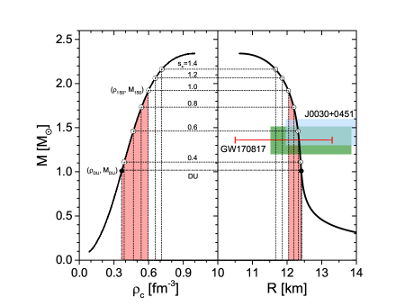
In order to illustrate the bulk properties of the V18 EOS thus obtained, Figure 1 shows the resulting NS mass-radius and mass-central density relations obtained in the standard way by solving the TOV equations for betastable and charge-neutral matter. We remark that the value of the maximum mass of the V18 EOS is larger than the current observational lower limits Demorest et al. (2010); Antoniadis et al. (2013); Fonseca et al. (2016); Cromartie et al. (2019). Regarding the radius, we found in Reference Burgio et al. (2018); Wei et al. (2019) that for the V18 EOS km, which fulfils the constraints derived from the tidal deformability in the GW170817 merger event, km Abbott et al. (2018), see also similar compatible constraints on masses and radii derived in References Margalit and Metzger (2017); Ruiz et al. (2018); Most et al. (2018); Rezzolla et al. (2018); Shibata et al. (2019); Most et al. (2020); Shao et al. (2020). The V18 EOS is also compatible with estimates of the mass and radius of the isolated pulsar PSR J0030+0451 observed recently by NICER, and km Miller et al. (2019), or and km Riley et al. (2019). The figure also shows the density of the onset of direct Urca (DU) cooling, , and the one of the vanishing of the p1S0 BCS gap, , to be introduced and discussed in the following, along with the pairing parameter .
2.2 Nuclear Cooling Processes
One of the main cooling regulators, besides the electromagnetic radiation from the surface, is the neutrino emission from the NS core. For sufficiently hot NSs the latter is in fact the main ingredient of the NS cooling theory Yakovlev et al. (2001); Page and Reddy (2006); Page et al. (2006); Lattimer and Prakash (2007); Potekhin et al. (2015). Several different neutrino generation processes are possible inside NSs, and their rates strongly depend on the NS EOS and composition and, very important, on the superfluid properties of the stellar matter, that is, critical temperatures and gaps in the different pairing channels. For instance, in a non-superfluid NS, the most powerful mechanism of neutrino emission is the direct Urca (DU) process, which consists of a pair of charged weak-current reactions,
| (6) |
where is a lepton, electron or muon, and is the corresponding neutrino. Those reactions are allowed by energy and momentum conservation Lattimer et al. (1991) only if , where is the Fermi momentum of the species . This implies that the proton fraction should be sufficiently high for the DU process to take place, and therefore the NS central density should be larger than some threshold density. Thus different EOSs predict different DU threshold densities.
For some EOSs, DU processes are forbidden in all NSs up to the most massive ones, and then other reactions come into play. In this case the basic neutrino emission mechanisms involve nucleon collisions, the strongest one being the modified Urca (MU) process,
| (7) |
where is a spectator nucleon that ensures momentum conservation. The nucleon-nucleon bremsstrahlung (BS) reactions,
| (8) |
with a nucleon and , an (anti)neutrino of any flavor, are also abundant in NS cores, and their rate increases with the baryon density, but they are orders of magnitude less powerful than the DU ones, thus producing a slow cooling Yakovlev et al. (2001).
For the V18 EOS used in this work, the DU process sets in at a proton fraction corresponding to a nucleon density of beta-stable and charge-neutral matter, and an associated NS mass , as indicated in Figure 1. Therefore practically all NSs can potentially cool very fast and slow cooling has to be achieved by superfluid suppression.
2.3 Pairing Gaps and Critical Temperatures
The neutrino cooling processes in NSs can be dramatically affected by the neutron and proton superfluidity Yakovlev et al. (2001); Sedrakian and Clark (2019), and the knowledge of the pairing gaps in the 1S0 and 3PF2 channels in beta-stable matter is essential for a correct description of the thermal evolution of a NS. These superfluids are produced by the and Cooper pairs formation due to the attractive part of the NN potential, and are characterized by a critical temperature for isotropic gaps. The occurrence of pairing leads to two relevant effects in NS cooling, namely (i) a strong reduction when of the emissivity of the neutrino processes the paired component is involved in, with a corresponding reduction of the specific heat of that component; (ii) onset of the “Cooper pair breaking and formation” (PBF) process with associated neutrino-antineutrino pair emission. This process starts when the temperature reaches of a given type of baryons, becomes maximally efficient when , and then is exponentially suppressed for Yakovlev et al. (2001). As usual, we focus in this work on the most important proton 1S0 (p1S0) and neutron 3PF2 (n3P2) pairing channels, while the n1S0 (crust only) gap is much less relevant for the cooling Wei et al. (2020), and the p3P2 gap is disregarded due to its uncertain properties at extreme densities.
In the simplest BCS approximation, and detailing the more general case of pairing in the coupled 3PF2 channel, the pairing gaps are computed by solving the (angle-averaged) gap equation Amundsen and Østgaard (1985); Baldo et al. (1992); Takatsuka and Tamagaki (1993); Elgarøy et al. (1996); Khodel et al. (1998); Baldo et al. (1998) for the two-component gap function,
| (9) |
with
| (10) |
while fixing the (neutron or proton) density,
| (11) |
Here is the s.p. energy, is the chemical potential determined self-consistently from Equations (9)–(11), and
| (12) |
are the relevant potential matrix elements ( and ; for the 3PF2 channel, ; for the 1S0 channel) with the bare potential . The relation between (angle-averaged) pairing gap at zero temperature obtained in this way and the critical temperature of superfluidity is then . (If no angle average is performed, the prefactor varies slightly, see, for example, References Yakovlev et al. (1999, 2001), but the angle-average procedure is usually an excellent approximation Baldo et al. (1992); Papakonstantinou and Clark (2017)).
However, in-medium effects might strongly modify these BCS results, as both the s.p. energy and the interaction kernel itself might include the effects of TBF and polarization corrections. It turns out that in the p1S0 channel all these corrections lead to a suppression of both magnitude and density domain of the BCS gap, see, for example, Figure 3 in Reference Zhou et al. (2004) and Figure 3 in Reference Baldo and Schulze (2007) in the BHF context, or Figure 7 in Reference Sedrakian and Clark (2019) and Figure 7 in Reference Lombardo and Schulze (2001) for a collection of different theoretical approaches, while for the n3P2 channel both TBF and polarization effects on might be attractive and change the value of the gaps even by orders of magnitude Khodel et al. (2004); Schwenk and Friman (2004); Ding et al. (2016). However, due to the high-density nature of this pairing, all medium effects might be very strong and there is still no reliable quantitative theoretical prediction for this gap.
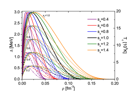
We anticipate, however, that nonzero values of the n3P2 gap cannot reproduce the current observational data in our cooling simulations, so that we exclude it ad-hoc from now on and concentrate our study on the possible p1S0 gap function . In this article we will not consider specific theoretical models for the various medium effects, but we use in the cooling simulations the density dependence of the 1S0 BCS pairing gap shown as solid black curve in Figure 2, modified by simple global scaling factors and on either magnitude and extension of the gap, that is,
| (13) |
The various trial gap functions are shown as colored curves in Figure 2 as a function of particle ( or ) density with different scale factors and applied. The unscaled gap () vanishes at . As just noted, theoretical calculations point to a reduction of both magnitude and density domain due to various in-medium effects for this type of pairing, which the scaling procedure attempts to mimic in a general way. Thus scaling factors larger than one appear very unrealistic. We include such choices only for the sake of a systematic investigation of their effect on the cooling. We now try to determine empirical optimal values of by comparing the theoretical results of our cooling simulations with the currently known cooling data.
2.4 Cooling Simulations
The NS cooling simulations are carried out using the widely known code NSCool Page (2010), which solves the general-relativistic equations of energy balance and energy transport,
| (14) | ||||
| (15) |
where is the metric function, , , and are the neutrino emissivity, the specific heat capacity, and the thermal conductivity, respectively. Local luminosity and temperature depend on radial coordinate and time . In order to compute them, the code adopts an implicit scheme (Henyey scheme) and solves the partial differential equations on a grid of spherical shells. The shell number is 1842 in this work. To facilitate the simulation, the star is divided artificially at a outer boundary with the radius and density . At , the matter is strongly degenerate and thus the structure of the star is supposed to be unchanged with the time. The envelope () includes the mass and composition change, for instance, due to the accretion, and is solved separately in the code. Here, we use the envelope model obtained by Potekhin Potekhin et al. (1997). Each simulation starts with a constant initial temperature profile, K, and ends when drops to K. Regarding the most important ingredient – neutrino emissivity, this code comprises all relevant cooling reactions: nucleonic DU, MU, PBF, and BS, including modifications due to p1S0 and n3P2 pairing. Moreover, various processes in the crust are included, such as the most important electron-nucleus bremsstrahlung, plasmon decay, electron-ion bremsstrahlung, and so forth.
3 Results
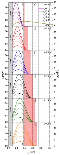
Due to the density-dependent proton fraction, the gap curves shown in Figure 2 correspond to much wider domains of baryon density for the p1S0 gap in NS matter that are shown in Figure 3. That figure also indicates the central densities for several NS masses (vertical lines) and the mass ranges (shaded red regions) in which DU cooling is suppressed by the p1S0 gap. Varying the parameter thus allows to regulate the NS mass domain of DU blocking, as was also indicated in Figure 1. For the BCS case, , the p1S0 gap disappears at , corresponding to , whereas the values for other scale factors are listed in Table 1. From theoretical investigations Zhou et al. (2004); Baldo and Schulze (2007); Lombardo and Schulze (2001); Sedrakian and Clark (2019) values of seem unrealistic, but are nevertheless included in our systematic analysis. For comparison also the unscaled n3P2 V18 BCS gap is shown in the figure. It extends over the entire density (mass) range and therefore also would block DU cooling for all NSs. However, the competing n3P2 PBF process provides too strong cooling for old objects, in disagreement with some data, as will be seen later.
| 0.2 | 0.4 | 0.6 | 0.8 | 1.0 | 1.2 | 1.4 | 1.6 | 1.8 | 2.0 | 2.5 | 3.0 | |
|---|---|---|---|---|---|---|---|---|---|---|---|---|
| 0.300 | 0.388 | 0.467 | 0.536 | 0.599 | 0.658 | 0.713 | 0.767 | 0.818 | 0.869 | 0.992 | 1.114 | |
| [] | 0.70 | 1.11 | 1.46 | 1.73 | 1.92 | 2.06 | 2.16 | 2.23 | 2.28 | 2.31 | 2.34 | 2.34 |
In Figure 4 we show the cooling diagrams, luminosity vs age, for several sets of interest, containing also the currently known data points with large (estimated) error bars, see Reference Beznogov and Yakovlev (2015). (We do not yet utilize the very recent update of these data Potekhin et al. (2020) in this work.) Theoretical results employing a Fe atmosphere (solid curves) and those with a light-elements atmosphere (dashed curves) are compared. Starting with the absence of superfluidity (a), , that is, DU cooling active for all NSs with , one obtains clearly unrealistic results so that this scenario can be excluded. Employing the original BCS values (b), , yields instead very reasonable results. In this case only high-mass stars, , cool very rapidly, whereas the cooling curves for lower masses are smoothly distributed in the plot, and not in apparent disaccordance with the data points. Note that in this case all known cooling objects can be explained, by assuming either a Fe or a light-elements atmosphere in specific cases, even the very hot XMMU J1731-347, (, ), which is indeed supposed to have a carbon atmosphere, as discussed in References Beznogov and Yakovlev (2015, 2015); Beznogov et al. (2018); Fortin et al. (2018). The third set (c), , is an optimal choice according to the mass-distribution analysis presented in the following. The difference to the BCS case is not very significant and again all data can be covered.
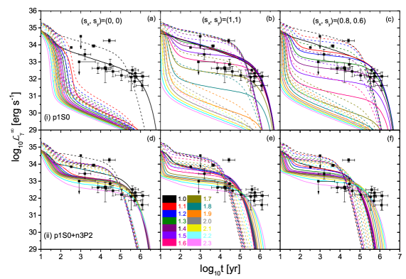
While the upper-row panels (a,b,c) employ only the p1S0 gap, the lower row (d,e,f) includes also the n3P2 BCS gap. In this case, however, cooling is too fast due to the very efficient PBF process of this channel, see a detailed discussion in Reference Wei et al. (2020), and the luminosity of old (yr) NSs cannot be reproduced. This problem also persists when allowing scale factors for this channel Taranto et al. (2016); Fortin et al. (2018). The same conclusions were drawn by References Beznogov and Yakovlev (2015, 2015); Potekhin et al. (2019, 2020) and other authors.
We remark that the approach presented here is able to describe perfectly with the same microphysics input not only the cooling of isolated NSs discussed here, but also the cooling of reheated accreting NSs in X-ray transients in quiescence (XRTQ) Yakovlev and Pethick (2004); Beznogov and Yakovlev (2015, 2015), as shown in Reference Fortin et al. (2018). We also remind the possible strong constraints on NS cooling imposed by the speculated very rapid cooling of the supernova remnant Cas A Ho and Heinke (2009); Heinke and Ho (2010); Elshamouty et al. (2013); Ho et al. (2015), which we have studied in detail in Reference Taranto et al. (2016). As the observational claims remain highly debated Posselt et al. (2013); Posselt and Pavlov (2018), we do not consider this scenario in this work.
The use of the V18 EOS together with the p1S0 BCS gap and no n3P2 pairing appears thus to be consistent with the current set of cooling data. However, without information on the actual masses of the various data points, it is currently impossible to perform a rigid check of the model by comparing the theoretically predicted masses with the actual masses of the data points in the cooling diagram. In the absence of this possibility we dedicate this work to another consistency check, namely the theoretical derivation of the NS mass distribution of the currently available data points from their position among the theoretical cooling curves for different masses. This mass distribution can then be compared to mass distributions of NSs obtained in different, independent theoretical ways Zhang et al. (2011); Özel et al. (2012); Kiziltan et al. (2013); Antoniadis et al. (2016); Alsing et al. (2018); Rocha et al. (2019).
Of course the validity of this analysis rests on two essential assumptions:
-
(a)
there is no bias on the masses (and thus luminosities) in the current data set of isolated NSs, that is, bright and dim objects are supposed to be present with equal probability, thus the detection of these sources is independent of their brightness;
-
(b)
the mass distribution of isolated NSs in the cooling diagram is not different from the mass distributions of NSs in binary systems Zhang et al. (2011); Antoniadis et al. (2016); Alsing et al. (2018); Rocha et al. (2019); Farrow et al. (2019) or all NSs in the Universe, which were addressed in the other theoretical studies.
Both of these assumptions are highly unlikely to be fulfilled, but are currently impossible to further scrutinize quantitatively. We therefore proceed with our derivation of the mass distribution of the current data as outlined above. The masses of the 19 cooling data points are assumed to be those predicted theoretically by their position in the cooling diagrams among the theoretical curves, see, for example, Figure 4 (neglecting any error bars at this stage of investigation), and Figure 5 shows the resulting mass histograms for different choices of the parameters , and assuming either a common Fe or a light-elements atmosphere for all data points. This is clearly unrealistic, and in fact in the first case only 15 and in the second case only 11 [apart from 10 for (0.6,0.2) and 12 for (1.4,0.8) and (1.4,1.0)] sources can be fitted, see Figure 4, while a fit of all data would require a suitable choice of atmosphere for each object. One observes that increasing or to a lesser degree shifts the centroid of the derived mass distribution to higher values, since the cooling curves like in Figure 4 shift upwards due to the increased suppression of the DU process.
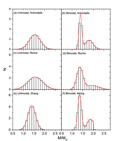
The different results in Figure 5 can now be compared with other theoretical studies of the NS mass distribution. There is a long-lasting discussion whether this distribution is unimodal or bimodal due to different classes of NS evolution histories Zhang et al. (2011); Özel et al. (2012); Kiziltan et al. (2013); Antoniadis et al. (2016); Alsing et al. (2018); Rocha et al. (2019), and in Figure 6 we show a compilation of some recent theoretical studies for the NS mass distribution. We provide a binning consistent with Figure 5 in order to compare directly with our results. For a quantitative comparison we simply compute the rms deviations between the histograms in Figure 6 and those in Figure 5. The results are given in Table 2 for the various combinations, where we also indicate the optimal values for each theoretical mass distribution and the two atmosphere models separately. Of course the use of a unique atmosphere model for the whole data set is unrealistic, but currently impossible to overcome without further constraints on the data.
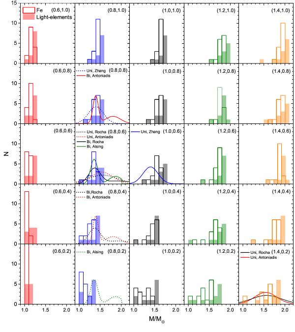
Nevertheless some qualitative conclusions can be drawn. Whereas for a Fe atmosphere a good agreement with some unimodal distributions seems to require fairly large (and unphysical) values of in order to shift the median to sufficiently large mass , most other cases indicate clearly preferred values of and , which would also be more consistent with microscopic investigations of the 1S0 pairing gap, as discussed before. The quality of agreement is only slightly better for unimodal distributions, but for too large . For a light-elements atmosphere, all theoretical models single out as preferred value, while is not well determined.
The () configurations which fit best a given theoretical model, have that theoretical curve superimposed in Figure 5, and four of the models (two unimodal, two bimodal) single out (0.8,0.6) as ‘best’ parameter set. Those values (0.8,0.6) were also used for some cooling diagrams shown in Figure 4. We conclude that in nearly all cases the comparison between cooling diagrams and population models indicates a reduction of the pairing range to and also a reduction of the magnitude , which is however less well determined and more model dependent. Both features are also supported by theoretical predictions for the 1S0 gap. The current limitations of theoretical method and available data do not allow to single out a preferred theoretical population model, though.
| Atmosphere | Fe | Light Elements | |||||||||
|---|---|---|---|---|---|---|---|---|---|---|---|
| 0.6 | 0.8 | 1.0 | 1.2 | 1.4 | 0.6 | 0.8 | 1.0 | 1.2 | 1.4 | ||
| Unimodal Antoniadis Antoniadis et al. (2016) | 1.0 | 2.46 | 2.28 | 2.22 | 1.96 | 2.61 | 2.09 | 1.39 | 1.54 | 1.60 | 1.36 |
| 0.8 | 2.69 | 1.77 | 1.56 | 2.07 | 2.20 | 1.95 | 1.23 | 1.33 | 1.79 | 1.53 | |
| 0.6 | 2.69 | 1.78 | 1.28 | 1.42 | 2.33 | 1.95 | 1.07 | 1.17 | 1.76 | 1.87 | |
| 0.4 | 3.29 | 1.83 | 1.31 | 1.28 | 1.78 | 1.78 | 1.55 | 1.48 | 1.43 | 1.90 | |
| 0.2 | 3.72 | 2.45 | 1.55 | 1.37 | 1.00 | 2.03 | 1.59 | 1.34 | 1.22 | 1.57 | |
| Unimodal Rocha Rocha et al. (2019) | 1.0 | 1.92 | 1.99 | 1.94 | 1.57 | 2.03 | 1.64 | 1.23 | 1.26 | 1.17 | 1.38 |
| 0.8 | 2.12 | 1.54 | 1.43 | 1.69 | 1.68 | 1.50 | 1.08 | 1.10 | 1.36 | 1.23 | |
| 0.6 | 2.11 | 1.49 | 1.22 | 1.65 | 1.85 | 1.48 | 0.86 | 1.43 | 1.35 | 1.42 | |
| 0.4 | 2.63 | 1.45 | 1.22 | 1.14 | 1.41 | 1.54 | 1.29 | 1.27 | 1.06 | 1.41 | |
| 0.2 | 3.00 | 1.90 | 1.20 | 1.20 | 0.90 | 1.18 | 1.34 | 1.13 | 0.95 | 1.19 | |
| Unimodal Zhang Zhang et al. (2011) | 1.0 | 2.37 | 2.48 | 2.48 | 2.61 | 2.80 | 1.97 | 1.48 | 2.12 | 2.17 | 2.28 |
| 0.8 | 2.68 | 1.61 | 1.95 | 2.71 | 1.95 | 1.86 | 1.29 | 1.92 | 2.34 | 2.08 | |
| 0.6 | 2.74 | 1.76 | 1.10 | 2.54 | 2.42 | 1.86 | 1.33 | 1.77 | 2.29 | 2.28 | |
| 0.4 | 3.38 | 1.45 | 1.14 | 1.90 | 2.15 | 1.77 | 1.38 | 1.65 | 2.06 | 2.33 | |
| 0.2 | 3.81 | 2.47 | 1.29 | 1.22 | 1.40 | 2.15 | 1.51 | 1.47 | 1.78 | 2.09 | |
| Bimodal Antoniadis Antoniadis et al. (2016) | 1.0 | 3.22 | 1.92 | 3.15 | 2.56 | 3.00 | 3.32 | 2.55 | 2.68 | 2.52 | 2.15 |
| 0.8 | 3.43 | 1.09 | 2.54 | 2.72 | 2.62 | 3.18 | 2.23 | 2.49 | 2.75 | 2.36 | |
| 0.6 | 3.40 | 1.30 | 2.24 | 2.19 | 2.83 | 3.18 | 1.87 | 2.39 | 2.61 | 2.69 | |
| 0.4 | 3.95 | 1.99 | 1.72 | 2.29 | 2.43 | 3.00 | 1.84 | 2.70 | 2.49 | 2.83 | |
| 0.2 | 4.37 | 3.17 | 1.76 | 1.90 | 1.58 | 3.24 | 2.05 | 2.55 | 2.37 | 2.45 | |
| Bimodal Rocha Rocha et al. (2019) | 1.0 | 2.11 | 1.80 | 2.46 | 2.19 | 2.51 | 1.67 | 1.40 | 1.82 | 1.70 | 1.77 |
| 0.8 | 2.40 | 1.14 | 1.88 | 2.31 | 2.21 | 1.57 | 1.22 | 1.64 | 1.90 | 1.69 | |
| 0.6 | 2.45 | 1.09 | 1.53 | 2.23 | 2.39 | 1.57 | 1.25 | 1.51 | 1.85 | 1.88 | |
| 0.4 | 3.03 | 1.20 | 1.19 | 1.73 | 2.01 | 1.50 | 1.21 | 1.54 | 1.67 | 1.85 | |
| 0.2 | 3.42 | 2.20 | 1.09 | 1.17 | 1.28 | 1.86 | 1.21 | 1.36 | 1.50 | 1.68 | |
| Bimodal Alsing Alsing et al. (2018) | 1.0 | 3.49 | 2.66 | 3.91 | 3.11 | 3.47 | 2.76 | 2.64 | 2.84 | 2.52 | 2.21 |
| 0.8 | 3.89 | 1.53 | 3.21 | 3.32 | 3.07 | 2.66 | 2.37 | 2.61 | 2.76 | 2.41 | |
| 0.6 | 3.94 | 1.20 | 2.81 | 2.74 | 3.34 | 2.66 | 2.08 | 2.50 | 2.62 | 2.64 | |
| 0.4 | 4.62 | 1.69 | 2.29 | 2.87 | 2.89 | 2.66 | 2.14 | 2.80 | 2.56 | 2.72 | |
| 0.2 | 5.12 | 3.58 | 1.86 | 2.13 | 2.19 | 3.16 | 1.68 | 2.58 | 2.46 | 2.46 | |
4 Conclusions
In this model study we have investigated the important effect of neutron and proton pairing gaps on NS cooling, which suppress the dominant DU process and open the competing PBF cooling reactions. For the betastable matter and resulting NS structure we used a fixed microscopically-derived BHF EOS that fulfils all current phenomenological constraints. This EOS features DU cooling for practically all NSs, which has to be (partially) quenched by superfluidity.
However, neutron 3P2 pairing leads to too rapid cooling of old NSs by the PBF process in contrast to several known objects and has to be excluded within this model, while proton 1S0 pairing together with an adjustment of the NS atmosphere is able to provide a satisfactory description of all current data. We then computed the derived NS mass distribution of the present set of data points from the cooling diagrams as a functional of the proton 1S0 gap, by scaling both the magnitude and the density domain of the BCS gap. In this way optimal scale factors (pointing to a reduction of both magnitude and density domain) and a optimal gap function could be obtained by reproducing a given theoretical mass distribution. The analysis yields a reasonable agreement with current theoretical bimodal mass distributions, due to the fact that the dominant peak is located at lower mass than in the unimodal distributions. However, unique atmosphere models for all sources had to be assumed in this setup.
Thus, at the current status of observational data from isolated NSs (few data points with large errors, not providing essential information on the NS masses and atmospheres), as well as an equally uncertain theoretical mass distribution of isolated NSs, this work can only be a ‘proof of concept’ study within our approach (following the works of Beznogov and Yakovlev (2015, 2015); Beznogov et al. (2018)) that demonstrates the potential that high-quality data would have to constrain the combination of nuclear bulk EOS and superfluid gaps in the future. This would complement the constraints obtained from other sources (on masses, radii, deformability, glitches, etc.) and ultimately allow the identification of the ‘unique’ NS EOS and superfluid properties of nuclear matter. With always more precise satellite observations, this goal might be achievable in the future.
All authors contributed to this work. All authors have read and agreed to the published version of the manuscript.
This work was partially funded by “PHAROS” COST Action CA16214 and the China Scholarship Council, No. 201706410092.
Acknowledgements.
We acknowledge helpful communication with D. Page. \conflictsofinterestThe authors declare no conflicts of interest. \reftitleReferencesReferences
- Yakovlev et al. (2001) Yakovlev, D.G.; Kaminker, A.D.; Gnedin, O.Y.; Haensel, P. Neutrino emission from neutron stars. Phys. Rep. 2001, 354, 1–155.
- Yakovlev and Pethick (2004) Yakovlev, D.G.; Pethick, C.J. Neutron Star Cooling. ARA&A 2004, 42, 169–210.
- Haskell and Sedrakian (2018) Haskell, B.; Sedrakian, A., Superfluidity and Superconductivity in Neutron Stars. In Astrophysics and Space Science Library; Springer: Berlin/Heidelberg, Germany, 2018; Volume 457, p. 401.
- Sedrakian and Clark (2019) Sedrakian, A.; Clark, J.W. Superfluidity in nuclear systems and neutron stars. EPJA 2019, 55, 167.
- Abbott et al. (2017) Abbott, B.P.; Abbott, R.; Abbott, T.D.; Acernese, F.; Ackley, K.; Adams, C.; Adams, T.; Addesso, P.; Adhikari, R.X.; Adya, V.B.; et al. GW170817: Observation of Gravitational Waves from a Binary Neutron Star Inspiral. Phys. Rev. Lett. 2017, 119, 161101.
- Abbott et al. (2018) Abbott, B.P.; Abbott, R.; Abbott, T.D.; Acernese, F.; Ackley, K.; Adams, C.; Adams, T.; Addesso, P.; Adhikari, R.X.; Adya, V.B.; et al. GW170817: Measurements of Neutron Star Radii and Equation of State. Phys. Rev. Lett. 2018, 121, 161101.
- Abbott et al. (2019) Abbott, B.P.; Abbott, T.D.; Acernese, F.; Ackley, K.; Adams, C.; Adams, T.; Addesso, P.; Adhikari, R.X.; Adya, V.B.; Affeldt, C.; et al. Properties of the Binary Neutron Star Merger GW170817. Phys. Rev. X 2019, 9, 011001.
- Taranto et al. (2016) Taranto, G.; Burgio, G.F.; Schulze, H.J. Cassiopeia A and direct Urca cooling. MNRAS 2016, 456, 1451–1458.
- Fortin et al. (2018) Fortin, M.; Taranto, G.; Burgio, G.F.; Haensel, P.; Schulze, H.J.; Zdunik, J.L. Thermal states of neutron stars with a consistent model of interior. MNRAS 2018, 475, 5010–5022.
- Wei et al. (2019) Wei, J.B.; Burgio, G.F.; Schulze, H.J. Neutron star cooling with microscopic equations of state. MNRAS 2019, 484, 5162–5169.
- Wei et al. (2020) Wei, J.B.; Burgio, G.F.; Schulze, H.J.; Zappalà, D. Cooling of hybrid neutron stars with microscopic equations of state. MNRAS 2020, doi:10.1093/mnras/staa1879.
- Beznogov and Yakovlev (2015) Beznogov, M.V.; Yakovlev, D.G. Statistical theory of thermal evolution of neutron stars. MNRAS 2015, 447, 1598–1609.
- Potekhin et al. (2020) Potekhin, A.Y.; Zyuzin, D.A.; Yakovlev, D.G.; Beznogov, M.V.; Shibanov, Y.A. Thermal luminosities of cooling neutron stars. MNRAS 2020, 496, 5052–5071.
- Jeukenne et al. (1976) Jeukenne, J.P.; Lejeune, A.; Mahaux, C. Many-body theory of nuclear matter. Phys. Rep. 1976, 25, 83–174.
- Baldo (1999) Baldo, M. Nuclear Methods And The Nuclear Equation of State; World Scientific: Singapore, 1999; Volume 8.
- Baldo and Burgio (2012) Baldo, M.; Burgio, G.F. Properties of the nuclear medium. Rep. Prog. Phys. 2012, 75, 026301.
- Song et al. (1998) Song, H.; Baldo, M.; Giansiracusa, G.; Lombardo, U. Bethe-Brueckner-Goldstone Expansion in Nuclear Matter. Phys. Rev. Lett. 1998, 81, 1584–1587.
- Baldo et al. (2000) Baldo, M.; Giansiracusa, G.; Lombardo, U.; Song, H.Q. Bethe-Brueckner-Goldstone expansion in neutron matter. Phys. Lett. B 2000, 473, 1–5.
- Lu et al. (2017) Lu, J.J.; Li, Z.H.; Chen, C.Y.; Baldo, M.; Schulze, H.J. Convergence of the hole-line expansion with modern nucleon-nucleon potentials. Phys. Rev. C 2017, 96, 044309.
- Lu et al. (2018) Lu, J.J.; Li, Z.H.; Chen, C.Y.; Baldo, M.; Schulze, H.J. Neutron matter in the hole-line expansion. Phys. Rev. C 2018, 98, 064322.
- Wiringa et al. (1995) Wiringa, R.B.; Stoks, V.; Schiavilla, R. An accurate nucleon-nucleon potential with charge independence breaking. Phys. Rev. C 1995, 51, 38–51.
- Grangé et al. (1989) Grangé, P.; Lejeune, A.; Martzolff, M.; Mathiot, J.F. Consistent three-nucleon forces in the nuclear many-body problem. Phys. Rev. C 1989, 40, 1040–1060.
- Zuo et al. (2002) Zuo, W.; Lejeune, A.; Lombardo, U.; Mathiot, J.F. Microscopic three-body force for asymmetric nuclear matter. EPJA 2002, 14, 469–475.
- Li et al. (2008) Li, Z.; Lombardo, U.; Schulze, H.J.; Zuo, W. Consistent nucleon-nucleon potentials and three-body forces. Phys. Rev. C 2008, 77, 034316.
- Li and Schulze (2008) Li, Z.H.; Schulze, H.J. Neutron star structure with modern nucleonic three-body forces. Phys. Rev. C 2008, 78, 028801.
- Wei et al. (2020) Wei, J.B.; Lu, J.J.; Burgio, G.F.; Li, Z.H.; Schulze, H.J. Are nuclear matter properties correlated to neutron star observables? EPJA 2020, 56, 63.
- Baldo et al. (2014) Baldo, M.; Burgio, G.F.; Schulze, H.J.; Taranto, G. Nucleon effective masses within the Brueckner-Hartree-Fock theory: Impact on stellar neutrino emission. Phys. Rev. C 2014, 89, 048801.
- Negele and Vautherin (1973) Negele, J.W.; Vautherin, D. Neutron star matter at subnuclear densities. Nucl. Phys. A 1973, 207, 298–320.
- Baym et al. (1971) Baym, G.; Pethick, C.; Sutherland, P. The ground state of matter at high densities: Equation of state and stellar models. ApJ 1971, 170, 299–317.
- Feynman et al. (1949) Feynman, R.P.; Metropolis, N.; Teller, E. Equations of State of Elements Based on the Generalized Fermi-Thomas Theory. Phys. Rev. 1949, 75, 1561–1573.
- Burgio and Schulze (2010) Burgio, G.F.; Schulze, H.J. The maximum and minimum mass of protoneutron stars in the Brueckner theory. A&A 2010, 518, A17.
- Baldo et al. (2014) Baldo, M.; Burgio, G.F.; Centelles, M.; Sharma, B.K.; Viñas, X. From the crust to the core of neutron stars on a microscopic basis. Phys. At. Nucl. 2014, 77, 1157–1165.
- Fortin et al. (2016) Fortin, M.; Providência, C.; Raduta, A.R.; Gulminelli, F.; Zdunik, J.L.; Haensel, P.; Bejger, M. Neutron star radii and crusts: Uncertainties and unified equations of state. Phys. Rev. C 2016, 94, 035804.
- Tsang et al. (2019) Tsang, C.Y.; Tsang, M.B.; Danielewicz, P.; Fattoyev, F.J.; Lynch, W.G. Insights on Skyrme parameters from GW170817. Phys. Lett. B 2019, 796, 1–5.
- Demorest et al. (2010) Demorest, P.B.; Pennucci, T.; Ransom, S.M.; Roberts, M.S.; Hessels, J.W. A two-solar-mass neutron star measured using Shapiro delay. Nature 2010, 467, 1081–1083.
- Antoniadis et al. (2013) Antoniadis, J.; Freire, P.C.C.; Wex, N.; Tauris, T.M.; Lynch, R.S.; van Kerkwijk, M.H.; Kramer, M.; Bassa, C.; Dhillon, V.S.; Driebe, T.; et al. A Massive Pulsar in a Compact Relativistic Binary. Science 2013, 340, 6131.
- Fonseca et al. (2016) Fonseca, E.; Pennucci, T.T.; Ellis, J.A.; Stairs, I.H.; Nice, D.J.; Ransom, S.M.; Demorest, P.B.; Arzoumanian, Z.; Crowter, K.; Dolch, T.; et al. The NANOGrav Nine-year Data Set: Mass and Geometric Measurements of Binary Millisecond Pulsars. ApJ 2016, 832, 167.
- Cromartie et al. (2019) Cromartie, H.T.; Fonseca, E.; Ransom, S.M.; Demorest, P.B.; Arzoumanian, Z.; Blumer, H.; Brook, P.R.; DeCesar, M.E.; Dolch, T.; Ellis, J.A.; et al. Relativistic Shapiro delay measurements of an extremely massive millisecond pulsar. Nat. Astron. 2019, 4, 72–76.
- Burgio et al. (2018) Burgio, G.F.; Drago, A.; Pagliara, G.; Schulze, H.J.; Wei, J.B. Are Small Radii of Compact Stars Ruled out by GW170817/AT2017gfo? ApJ 2018, 860, 139.
- Wei et al. (2019) Wei, J.B.; Figura, A.; Burgio, G.F.; Chen, H.; Schulze, H.J. Neutron star universal relations with microscopic equations of state. J. Phys. G: Nucl. Part. Phys. 2019, 46, 034001.
- Margalit and Metzger (2017) Margalit, B.; Metzger, B.D. Constraining the Maximum Mass of Neutron Stars from Multi-messenger Observations of GW170817. ApJ 2017, 850, L19.
- Ruiz et al. (2018) Ruiz, M.; Shapiro, S.L.; Tsokaros, A. GW170817, general relativistic magnetohydrodynamic simulations, and the neutron star maximum mass. Phys. Rev. D 2018, 97, 021501.
- Most et al. (2018) Most, E.R.; Weih, L.R.; Rezzolla, L.; Schaffner-Bielich, J. New constraints on radii and tidal deformabilities of neutron stars from GW170817. Phys. Rev. Lett. 2018, 120, 261103.
- Rezzolla et al. (2018) Rezzolla, L.; Most, E.R.; Weih, L.R. Using Gravitational-wave Observations and Quasi-universal Relations to Constrain the Maximum Mass of Neutron Stars. ApJ 2018, 852, L25.
- Shibata et al. (2019) Shibata, M.; Zhou, E.; Kiuchi, K.; Fujibayashi, S. Constraint on the maximum mass of neutron stars using GW170817 event. Phys. Rev. D 2019, 100, 023015.
- Most et al. (2020) Most, E.R.; Papenfort, L.J.; Weih, L.R.; Rezzolla, L. A lower bound on the maximum mass if the secondary in GW190814 was once a rapidly spinning neutron star. arXiv 2020, arXiv:2006.14601.
- Shao et al. (2020) Shao, D.S.; Tang, S.P.; Sheng, X.; Jiang, J.L.; Wang, Y.Z.; Jin, Z.P.; Fan, Y.Z.; Wei, D.M. Estimating the maximum gravitational mass of nonrotating neutron stars from the GW170817/GRB 170817A/AT2017gfo observation. Phys. Rev. D 2020, 101, 063029.
- Miller et al. (2019) Miller, M.C.; Lamb, F.K.; Dittmann, A.J.; Bogdanov, S.; Arzoumanian, Z.; Gendreau, K.C.; Guillot, S.; Harding, A.K.; Ho, W.C.G.; Lattimer, J.M.; et al. PSR J00300451 Mass and Radius from NICER Data and Implications for the Properties of Neutron Star Matter. ApJ 2019, 887, L24.
- Riley et al. (2019) Riley, T.E.; Watts, A.L.; Bogdanov, S.; Ray, P.S.; Ludlam, R.M.; Guillot, S.; Arzoumanian, Z.; Baker, C.L.; Bilous, A.V.; Chakrabarty, D.; et al. A NICER View of PSR J00300451: Millisecond Pulsar Parameter Estimation. ApJ 2019, 887, L21.
- Page and Reddy (2006) Page, D.; Reddy, S. Dense Matter in Compact Stars: Theoretical Developments and Observational Constraints. Annu. Rev. Nucl. Part. Sci. 2006, 56, 327–374.
- Page et al. (2006) Page, D.; Geppert, U.; Weber, F. The cooling of compact stars. Nucl. Phys. A 2006, 777, 497–530.
- Lattimer and Prakash (2007) Lattimer, J.M.; Prakash, M. Neutron star observations: Prognosis for equation of state constraints. Phys. Rep. 2007, 442, 109–165.
- Potekhin et al. (2015) Potekhin, A.Y.; Pons, J.A.; Page, D. Neutron Stars–Cooling and Transport. Space Sci. Rev. 2015, 191, 239–291.
- Lattimer et al. (1991) Lattimer, J.M.; Pethick, C.J.; Prakash, M.; Haensel, P. Direct URCA process in neutron stars. Phys. Rev. Lett. 1991, 66, 2701–2704.
- Amundsen and Østgaard (1985) Amundsen, L.; Østgaard, E. Superfluidity of neutron matter (II). Triplet pairing. Nucl. Phys. A 1985, 442, 163–188.
- Baldo et al. (1992) Baldo, M.; Cugnon, J.; Lejeune, A.; Lombardo, U. Proton and neutron superfluidity in neutron star matter. Nucl. Phys. A 1992, 536, 349–365.
- Takatsuka and Tamagaki (1993) Takatsuka, T.; Tamagaki, R. Chapter II. Superfluidity in Neutron Star Matter and Symmetric Nuclear Matter. Prog. Theor. Phys. Suppl. 1993, 112, 27–65.
- Elgarøy et al. (1996) Elgarøy, Ø.; Engvik, L.; Hjorth-Jensen, M.; Osnes, E. Triplet pairing of neutrons in -stable neutron star matter. Nucl. Phys. A 1996, 607, 425–441.
- Khodel et al. (1998) Khodel, V.A.; Khodel, V.V.; Clark, J.W. Universalities of Triplet Pairing in Neutron Matter. Phys. Rev. Lett. 1998, 81, 3828–3831.
- Baldo et al. (1998) Baldo, M.; Elgarøy, Ø.; Engvik, L.; Hjorth-Jensen, M.; Schulze, H.J. 3P2-3F2 pairing in neutron matter with modern nucleon-nucleon potentials. Phys. Rev. C 1998, 58, 1921–1928.
- Yakovlev et al. (1999) Yakovlev, D.G.; Levenfish, K.P.; Shibanov, Y.A. Reviews of Topical Problems: Cooling of neutron stars and superfluidity in their cores. Phys. Uspekhi 1999, 42, 737–778.
- Papakonstantinou and Clark (2017) Papakonstantinou, P.; Clark, J.W. Three-Nucleon Forces and Triplet Pairing in Neutron Matter. J. Low Temp. Phys. 2017, 189, 361–382.
- Zhou et al. (2004) Zhou, X.R.; Schulze, H.J.; Zhao, E.G.; Pan, F.; Draayer, J.P. Pairing gaps in neutron stars. Phys. Rev. C 2004, 70, 048802.
- Baldo and Schulze (2007) Baldo, M.; Schulze, H.J. Proton pairing in neutron stars. Phys. Rev. C 2007, 75, 025802.
- Lombardo and Schulze (2001) Lombardo, U.; Schulze, H.J., Superfluidity in Neutron Star Matter. In Physics of Neutron Star Interiors; World Scientific: Singapore, 2001; Volume 578, p. 30.
- Khodel et al. (2004) Khodel, V.A.; Clark, J.W.; Takano, M.; Zverev, M.V. Phase Transitions in Nucleonic Matter and Neutron-Star Cooling. Phys. Rev. Lett. 2004, 93, 151101.
- Schwenk and Friman (2004) Schwenk, A.; Friman, B. Polarization Contributions to the Spin Dependence of the Effective Interaction in Neutron Matter. Phys. Rev. Lett. 2004, 92, 082501.
- Ding et al. (2016) Ding, D.; Rios, A.; Dussan, H.; Dickhoff, W.H.; Witte, S.J.; Carbone, A.; Polls, A. Pairing in high-density neutron matter including short- and long-range correlations. Phys. Rev. C 2016, 94, 025802.
- Page (2010) Page, D. NSCool Code. 2010. Available online: http://www.astroscu.unam.mx/neutrones/NSCool (accessed on 07/08/2020).
- Potekhin et al. (1997) Potekhin, A.; Chabrier, G.; Yakovlev, D. Internal temperatures and cooling of neutron stars with accreted envelopes. A&A 1997, 323, 415.
- Beznogov and Yakovlev (2015) Beznogov, M.V.; Yakovlev, D.G. Statistical theory of thermal evolution of neutron stars - II. Limitations on direct Urca threshold. MNRAS 2015, 452, 540–548.
- Beznogov et al. (2018) Beznogov, M.V.; Rrapaj, E.; Page, D.; Reddy, S. Constraints on axion-like particles and nucleon pairing in dense matter from the hot neutron star in HESS J1731-347. Phys. Rev. C 2018, 98, 035802.
- Potekhin et al. (2019) Potekhin, A.Y.; Chugunov, A.I.; Chabrier, G. Thermal evolution and quiescent emission of transiently accreting neutron stars. A&A 2019, 629, A88.
- Ho and Heinke (2009) Ho, W.C.G.; Heinke, C.O. A neutron star with a carbon atmosphere in the Cassiopeia A supernova remnant. Nature 2009, 462, 71–73.
- Heinke and Ho (2010) Heinke, C.O.; Ho, W.C.G. Direct Observation of the Cooling of the Cassiopeia A Neutron Star. ApJ 2010, 719, L167–L171.
- Elshamouty et al. (2013) Elshamouty, K.G.; Heinke, C.O.; Sivakoff, G.R.; Ho, W.C.G.; Shternin, P.S.; Yakovlev, D.G.; Patnaude, D.J.; David, L. Measuring the Cooling of the Neutron Star in Cassiopeia A with all Chandra X-ray Observatory Detectors. ApJ 2013, 777, 22.
- Ho et al. (2015) Ho, W.C.G.; Elshamouty, K.G.; Heinke, C.O.; Potekhin, A.Y. Tests of the nuclear equation of state and superfluid and superconducting gaps using the Cassiopeia A neutron star. Phys. Rev. C 2015, 91, 015806.
- Posselt et al. (2013) Posselt, B.; Pavlov, G.G.; Suleimanov, V.; Kargaltsev, O. New Constraints on the Cooling of the Central Compact Object in Cas A. ApJ 2013, 779, 186.
- Posselt and Pavlov (2018) Posselt, B.; Pavlov, G.G. Upper Limits on the Rapid Cooling of the Central Compact Object in Cas A. ApJ 2018, 864, 135.
- Özel et al. (2012) Özel, F.; Psaltis, D.; Narayan, R.; Santos Villarreal, A. On the Mass Distribution and Birth Masses of Neutron Stars. ApJ 2012, 757, 55.
- Kiziltan et al. (2013) Kiziltan, B.; Kottas, A.; De Yoreo, M.; Thorsett, S.E. The Neutron Star Mass Distribution. ApJ 2013, 778, 66.
- Zhang et al. (2011) Zhang, C.M.; Wang, J.; Zhao, Y.H.; Yin, H.X.; Song, L.M.; Menezes, D.P.; Wickramasinghe, D.T.; Ferrario, L.; Chardonnet, P. Study of measured pulsar masses and their possible conclusions. A&A 2011, 527, A83.
- Antoniadis et al. (2016) Antoniadis, J.; Tauris, T.M.; Özel, F.; Barr, E.; Champion, D.J.; Freire, P.C.C. The millisecond pulsar mass distribution: Evidence for bimodality and constraints on the maximum neutron star mass. arXiv 2016, arXiv:astro-ph.HE/1605.01665.
- Alsing et al. (2018) Alsing, J.; Silva, H.O.; Berti, E. Evidence for a maximum mass cut-off in the neutron star mass distribution and constraints on the equation of state. MNRAS 2018, 478, 1377–1391.
- Rocha et al. (2019) Rocha, L.S.; Bernardo, A.; Horvath, J.E.; Valentim, R.; de Avellar, M.G.B. The distribution of neutron star masses. Astron. Nachrichten 2019, 340, 957–963.
- Farrow et al. (2019) Farrow, N.; Zhu, X.J.; Thrane, E. The Mass Distribution of Galactic Double Neutron Stars. ApJ 2019, 876, 18.