An Empirical Study on Model-agnostic Debiasing Strategies
for Robust Natural Language Inference

Abstract

The prior work on natural language inference (NLI) debiasing mainly targets at one or few known biases while not necessarily making the models more robust. In this paper, we focus on the model-agnostic debiasing strategies and explore how to (or is it possible to) make the NLI models robust to multiple distinct adversarial attacks while keeping or even strengthening the models’ generalization power. We firstly benchmark prevailing neural NLI models including pretrained ones on various adversarial datasets. We then try to combat distinct known biases by modifying a mixture of experts (MoE) ensemble method Clark et al. (2019) and show that it’s nontrivial to mitigate multiple NLI biases at the same time, and that model-level ensemble method outperforms MoE ensemble method. We also perform data augmentation including text swap, word substitution and paraphrase and prove its efficiency in combating various (though not all) adversarial attacks at the same time. Finally, we investigate several methods to merge heterogeneous training data (1.35M) and perform model ensembling, which are straightforward but effective to strengthen NLI models.

1 Introduction

Natural language inference (NLI) (also known as recognizing textual entailment) is a widely studied task which aims to infer the relationship (e.g., entailment, contradiction, neutral) between two fragments of text, known as premise and hypothesis Dagan et al. (2005, 2013). Recent works have found that NLI models are sensitive to the compositional features Nie et al. (2019), syntactic heuristics McCoy et al. (2019), stress test Geiger et al. (2018); Naik et al. (2018) and human artifacts in the data collection phase Gururangan et al. (2018); Poliak et al. (2018b); Tsuchiya (2018). Accordingly, several adversarial datasets are proposed for these known biases.

Through our preliminary trials on specific adversarial datasets, we find that although the model specific or dataset specific debiasing methods could increase the model performance on the paired adversarial dataset, they might hinder the model performance on other adversarial datasets, as well as hurt the model generalization power, i.e. deficient scores on cross-datasets or cross-domain settings. These phenomena motivate us to investigate if it exists a unified model-agnostic debiasing strategy which can mitigate distinct (or even all) known biases while keeping or strengthening the model generalization power.

We begin with NLI debiasing models. To make our trials more generic, we adopt a mixture of experts (MoE) strategy Clark et al. (2019), which is known for being model-agnostic and is adaptable to various kinds of known biases, as backbone. Specifically we treat three known biases, namely word overlap, length mismatch and partial input heuristics as independent experts and train corresponding debiasing models. Our results show that the debiasing methods tied to one particular known bias may not be sufficient to build a generalized, robust model. This motivates us to investigate a better solution to integrate the advantages of distinct debiasing models. We find model-level ensemble is more effective than other MoE ensemble methods. Although our findings are based on the MoE backbone due to the prohibitive exhaustive studies on the all existing debiasing strategies, we provide actionable insights on combining distinct NLI debiasing methods to the practitioners.

Then we explore model agnostic and generic data augmentation methods in NLI, including text swap, word substitution and paraphrase. We find these methods could help NLI models combat multiple (though not all) adversarial attacks, e.g. augmenting training data by swapping hypothesis and premise could boost the model performance on stress tests and lexical inference test, and data augmentation by paraphrasing the hypothesis sentences could help the models resist the superficial patterns from syntactic and partial input heuristics. We also observe that increasing training size by incorporating heterogeneous training resources is a simple but effective method to build robust and generalized models. Specifically we investigate how to incorporate different training data with different sizes and annotation processes, as well as the best way to perform model ensembling.

Datasets	Paper	Categories	Labels	Size
PI-CD	(a)	$1\|3\|7$	(E,N,C)	3.2k
PI-SP	(b)	$1\|3\|7$	(E,N,C)	.37k
IS-SD	(c)	$2\|5\|8$	($\neg$E, E)	30k
IS-CS	(d)	$2\|3\|7$	(E,N,C)	.65k
LI-LI	(e)(f)	$2\|4\|9$	(E,C)	9.9K
LI-TS	(g)(h)	$2\|6\|10$	($\neg$C, C)	9.8K
ST-WO	(e)	$2\|4\|11$	(E,N,C)	9.8K
ST-NE	(e)	$2\|4\|11$	(E,N,C)	9.8K
ST-LM	(e)	$2\|4\|11$	(E,N,C)	9.8K
ST-SE	(e)	$2\|4\|12$	(E,N,C)	31K

(a) Gururangan et al. (2018)	(b) Liu et al. (2020)
(c) McCoy et al. (2019)	(d) Nie et al. (2019)
(e) Naik et al. (2018)	(f) Glockner et al. (2018)
(g) Wang et al. (2019c)	(h) Minervini and Riedel

Category	First-level	Second-level
1	$(\mathbf{I})$	Partial input heuristics
2	$(\mathbf{I})$	Inter-sentence heuristics
3	$(\mathbf{II})$	Instance selection
4	$(\mathbf{II})$	Single Sentence Modification
5	$(\mathbf{II})$	Sentence Pair Modification
6	$(\mathbf{II})$	Sentence Pair Swapping
7	$(\mathbf{III})$	Lexical Statistical Irregularity
8	$(\mathbf{III})$	Syntactic Statistical Irregularity
9	$(\mathbf{III})$	Lexical Inference
10	$(\mathbf{III})$	First Order Logic
11	$(\mathbf{III})$	Stress Test - Distraction Test
12	$(\mathbf{III})$	Stress Test - Noise Test

$(\mathbf{I})$ Where are the heuristics?
$(\mathbf{II})$ How did the dataset constructed?
$(\mathbf{III})$ Which aspect did the dataset detect?

Table 1: The information of adversarial datasets (Sec 2) we use in this paper. We categorize and rename these datasets as discussed in Sec 2.1.

2 Benchmark Datasets

Our benchmark datasets include the adversarial datasets and some widely used general-purpose NLI datasets which test the generalization power of NLI models.

2.1 Adversarial Datasets

Categorization: to provide more insights on how the adversarial datasets attack the models, we roughly categorize them in Table 1 according to their characteristics and elaborate the categorization in this section. To facilitate the narrative of following sections, we rename the adversarial datasets according to their prominent features.

Comparability: all the following datasets are collected based on the public available resources proposed by their authors, thus the experimental results in this paper are comparable to the numbers reported in the original papers and the other papers that use these datasets.

2.1.1 Partial-input (PI) Heuristics

Partial-input heuristics refer to the hypothesis-only bias Poliak et al. (2018b) in NLI.

Classifier Detected Datasets (PI-CD): Gururangan et al. (2018) trained a neural classifier (fastText) on the hypothesis sentences and then treated those instances in the SNLI test sets which can not be correctly classified as ‘hard’ instances.

Surface Pattern Datasets (PI-SP): Liu et al. (2020) recognized surface patterns which are highly correlated to the specific labels and correspondingly proposed adversarial test sets which are against surface patterns’ indications. We use their ‘hard’ instances for MultiNLI mismatched dev set as adversarial datasets.

2.1.2 Inter-sentences (IS) Heuristics

Syntactic Diagnostic Datasets (IS-SD): The HANS dataset McCoy et al. (2019) includes lexical overlap, subsequence and constituent heuristics between the hypothesis and premises sentences, e.g. the model might incorrectly predict ‘entailment’ for instance like ‘The actor was paid by the judge’ and ‘The actor paid the judge’.

Compositionality-sensitivity Datasets (IS-CS): Nie et al. (2019) trained a softmax regression model using unigram pattern pair features across two sentences as well as unigram features in hypothesis and premise sentences to obtain the ’lexically misleading scores (LMS)’ for each instance in the test sets. We use $\mathbf{CS}_{0.7}$ in their paper which denotes the subsets whose LMS are larger that 0.7.

2.1.3 Logical Inference Ability (LI)

Lexical Inference Test (LI-LI): A proper NLI system should recognize hypernyms and hyponyms; synonym and antonyms. We merge the “antonym” category in Naik et al. (2018) and Glockner et al. (2018) to assess the models’ capability to model lexical inference.

Text-fragment Swap Test (LI-TS): NLI system should also follow the first-order logic constraints Wang et al. (2019c); Minervini and Riedel (2018). For example, if the premise sentence $s_{p}$ entails the hypothesis sentence $s_{h}$, then $s_{h}$ must not be contradicted by $s_{p}$. We then swap the two sentences in the original MultiNLI mismatched dev sets. If the gold label is ‘contradiction’, the corresponding label in the swapped instance remains unchanged, otherwise it becomes ‘non-contradicted’.

2.1.4 Stress Test (ST)

We also include the “word overlap” (ST-WO), “negation” (ST-NE), “length mismatch” (ST-LM) and “spelling errors” (ST-SE) in Naik et al. (2018), in which ST-WO aims at detecting lexical overlap heuristics described in McCoy et al. (2019) (IS-SD in Sec 2.1.2); ST-NE aims at detecting strong negative lexical cues in partial-input sentences like PI-SP in Sec 2.1.2.

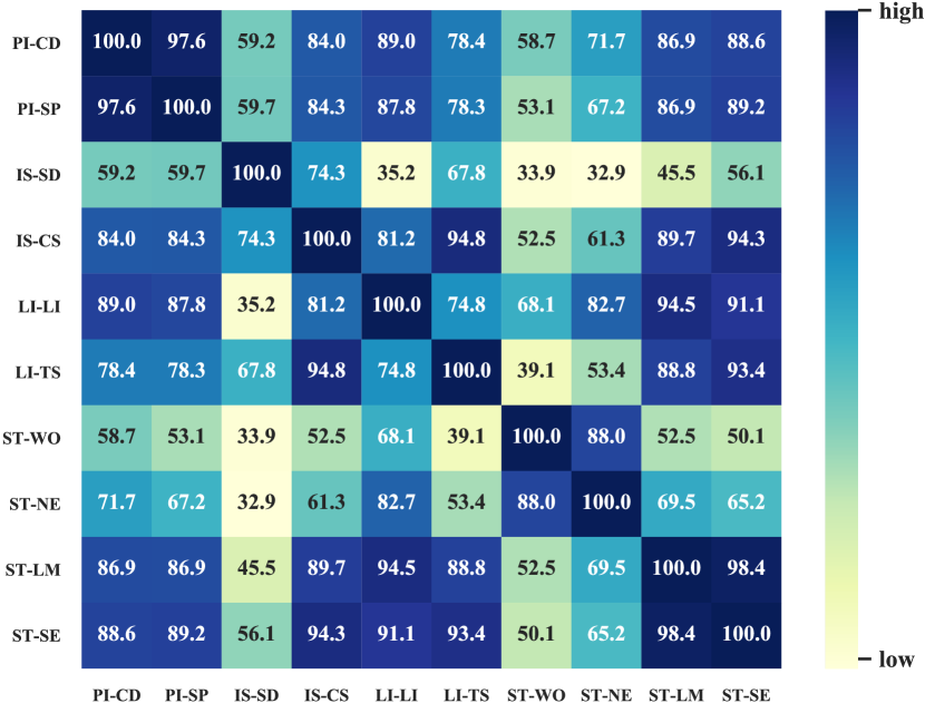
Figure 1: The surrogate correlations between different adversarial datasets. We show the Pearson’s correlation coefficients of model performance on different adversarial datasets in different runs (Sec 2.1.5).

2.1.5 Insights within Adversarial Tests

To provide actionable insights to NLP practitioners, we list how these adversarial instances constructed and why they might fail NLI models in Table 1. Those adversarial datasets are potentially correlated with each other due to similar constructing process or constructing goals. For example, ‘PI-CD’, ‘PI-SP’ and ‘IS-CS’ are all created with instance selection from original test sets in order to attack the models which improperly rely on the superficial lexical patterns, thus they might be potentially correlated. Although we could analytically assess the correlation between adversarial datasets, it is hard to demonstrate their underlying relationships from a quantitative perspective. We instead try to utilize the model performances on these adversarial datasets as surrogates to visualize their correlations. Concretely, we first collect the model accuracy scores on each adversarial dataset according to 30 runs of 10 baseline models (3 runs each) listed in Table 3. Then we show the pearson correlation coefficients of the model scores on any two distinct adversarial datasets in Fig 1. According to Fig 1, ‘IS-SD’ (HANS) has higher correlation with ‘IS-CS’ and ‘LI-TS’ compared with other adversarial datasets, we assume this is because they are constructed based on cross sentence heuristics in the natural occurring settings, as opposed to stress test datasets which add tautology like ‘and true is true’ to the end of hypothesis sentences Naik et al. (2018). ‘LI-LI’ instances are created by few lexical changes on premise sentence which would easily fall into ‘word overlap’ heuristics as elaborated in the ‘IS-SD’ dataset, thus ‘LI-LI’ has low correlation with ‘IS-SD’.

	SNLI	MNLI	DNLI	ANLI
Train	549362	392702	249947	162765
Valid	9842	9832	31696	2200
Test	9824	9815	31232	2200

Table 2: Statistics for datasets used in Sec 5. For MNLI, we utlize the matched dev and mismatched dev sets as valid and test sets respectively.

	Adversarial Test								Generalization Power Test
	PI-CD	PI-SP	IS-SD	IS-CS	LI-LI	LI-TS	ST	Avg.	RTE	DIAG	SICK	SciTail	Avg.	MNLI
InferSent	52.1	55.3	53.9	33.5	43.6	70.5	53.3	51.7	61.8	10.6	25.4	24.7	30.6	70.5
+ELMO	48.6	59.8	55.2	42.1	38.5	72.4	52.7	52.8	62.5	9.8	24.6	18.5	28.9	72.5
DAM	55.0	54.4	50.2	35.7	62.7	74.3	53.0	55.0	62.7	10.3	27.0	30.0	32.5	70.3
ESIM	55.1	66.3	49.8	52.7	63.2	79.6	53.8	60.1	66.2	11.3	25.1	27.5	32.5	77.3
$\mathrm{BERT}_{B}$	72.2	73.9	63.8	65.4	85.6	82.6	63.5	72.4	75.4	36.2	54.2	66.1	58.0	83.5
$\mathrm{BERT}_{L}$	74.7	75.5	70.4	70.6	87.9	83.8	67.3	75.7	77.6	39.4	55.5	68.3	60.2	85.7
$\mathrm{XLNet}_{B}$	73.1	77.9	71.2	70.4	85.5	84.8	68.5	75.9	78.0	39.2	55.8	66.7	59.9	86.6
$\mathrm{XLNet}_{L}$	78.8	81.7	76.7	77.3	93.4	88.5	72.4	81.3	83.4	45.9	57.6	73.0	65.0	89.3
$\mathrm{RoBERTa}_{B}$	76.6	80.9	72.0	74.1	89.6	85.3	66.4	77.8	80.9	42.1	55.9	69.0	62.0	87.4
$\mathrm{RoBERTa}_{L}$	80.0	79.2	80.0	77.0	92.4	88.6	73.4	81.5	84.4	50.5	57.3	72.2	66.1	89.9

Table 3: The performance of models on adversarial and generalization power tests (Sec 2) trained on MultiNLI. B and L in the subscript denote base and large versions of pretrained models. We use bold and underlined numbers to represent the highest scores in each column/block. Same marks are also used in Table 4, 5 and 6.

2.2 Other Data Resources

Generalization Power Test: we test the models on several general purpose datasets, including NLI diagnostic dataset (Diag) Wang et al. (2019b), for which we use ‘Matthews correlation coefficient’ Matthews (1975) as the evaluation metric. We also incorporate RTE Dagan et al. (2005), SICK Marelli et al. (2014) and SciTail Khot et al. (2018) in our testing.

Training Resources: apart from SNLI Bowman et al. (2015), and MultiNLI Williams et al. (2018), we also incorporate Diverse NLI (DNLI) Poliak et al. (2018a) and Adversarial NLI (ANLI) Nie et al. (2020) datasets for training. For DNLI, we merge the subsets to form unified train/valid/test sets. Dataset Statistics are shown in Table 2.

2.3 Model Performance on the Benchmark

We show the performance of different models trained on MultiNLI in Table 3. The general trend is that more powerful model which has higher performance on the original (in-domain) test sets (RoBERTa (large)) outperforms most models in both adversarial and general purpose settings.

In the following sections, we investigate several model agnostic methods for debiasing NLI models. Specifically, we are interested in: 1) how to (or is it possible to) make the NLI models robust to multiple distinct adversarial attacks using a unified debiasing method and 2) how the debiasing methods influence model generalization power of NLI.

	Baseline	Word Overlap		Partial Input		Sentence Length		Debiasing Combination
	($\mathrm{BERT}_{base}$)	ReW	BiasProd	ReW	BiasProd	ReW	BiasProd	MixW	AddProd	BestEn
PI-CD	72.2	70.9	71.4	72.6	71.8	72.6	72.3	71.9	71.3	72.6
PI-SP	73.9	70.6	70.1	74.7	73.0	75.2	73.3	71.7	70.4	73.9
IS-SD	63.8	69.2	71.0	65.7	63.8	56.9	59.5	54.6	61.5	72.5
IS-CS	65.4	64.8	64.2	67.1	68.9	64.9	66.9	65.4	68.9	64.9
LI-LI	85.6	87.0	87.8	86.0	85.0	85.7	85.5	86.8	88.4	87.7
LI-TS	82.6	81.8	81.7	82.0	82.3	81.3	83.7	82.3	81.9	84.5
ST-LM	82.2	82.3	81.7	81.6	81.1	82.6	82.7	82.6	79.9	83.1
Gen. Avg.	58.0	56.8	56.6	57.5	56.7	57.9	57.5	57.1	55.9	58.1
MNLI	83.5	84.2	82.8	84.3	83.3	80.3	80.9	84.0	81.2	84.5

Table 4: The performance of debiasing methods (Sec 3) based on BERT base model (baseline) trained on MultiNLI. ReW, BiasProd refer to instance reweighting and bias product ensemble methods in Sec 3.1. Word overlap, partial input and sentence length are the known biases in NLI (Sec 3.2). MixW, AddProd, BestEn are our trials to combine distinct debiasing methods (Sec 3.3). ‘Gen. Avg’ is the average score of test sets in generalization power test. Bold numbers mark the highest score (besting debiasing model) in each row.

3 Mixture of Experts (MoE) Debiasing

We utilize the MoE ensemble model Clark et al. (2019) as the backbone to mitigate three known biases in NLI. Concretely, we implement the ‘instance reweighting’ and ‘bias product’ methods in Clark et al. (2019). Based on these methods, we perform several trials on combating several distinct NLI biases at the same time.

3.1 Debiasing Methods

Notations: for a known NLI bias, they firstly train a bias-only model $B$ and then use its output $\mathbf{b}$ as a guidance to train the prime model. In the context of three-way NLI training, $\mathbf{b_{i}}$ is a normalized 3-element vector which represents the predicted possibility of each NLI label for i-th training example. Suppose $\mathbf{p_{i}}$ is output of the prime model which has the same meaning as $\mathbf{b_{i}}$.

Instance Reweighting: suppose $b_{i}^{y_{i}}$ is the possibility that the bias-only model assigns to the correct label $y_{i}$ for $i$-th training example. They trained the models in a weighted version of the data, where the weight $\alpha_{i}$ for the $i$-th training example is (1-$b_{i}^{y_{i}}$). The loss function for a training batch with $k$ examples is a weighted sum of instance-level loss $l_{i}$: $\mathbf{L}_{batch}=\alpha_{i}*l_{i}/(\sum_{i=1}^{k}\alpha_{i})$.

Bias Product Ensemble: an ensemble method that is a product of experts $\mathbf{\hat{p_{i}}}=softmax(log(\mathbf{p_{i}})+log(\mathbf{b_{i}}))$.

By doing so, the prime model would be encouraged to learn all the information except the specific bias. An intuitive justification from the probabilistic view can be found in Clark et al. (2019). Note that while training, only the prime model is updated while the bias-only model remains unchanged.

3.2 Known Biases in NLI

Word overlap heuristics: To combat the word overlap heuristics (HANS McCoy et al. (2019), renamed as IS-SD in Sec 2.1.2), Clark et al. (2019) used the following features to train a bias-only model: (1) whether the hypothesis is a sub-sequence of the premise, (2) whether all words in the hypothesis appear in the premise, (3) the percent of words from the hypothesis that appear in the premise, (4) the average and the max of the minimum distance between each premise word with each hypothesis word. We use their trained bias-only model output for experiments.

Partial input heuristics: To combat the hypothesis-only bias in NLI (PI-CD and PI-SP in Sec 2.1.1), we use RoBERTa (base) model to train a bias-only model by taking only hypothesis sentences as inputs. Our hypothesis-only model gets 60.4% accuracy on the mismatched dev set of MultiNLI, which is higher than the reported numbers in Gururangan et al. (2018) (52.3%) and Poliak et al. (2018b) (55.18%).

Sentence length heuristics: Gururangan et al. (2018) shows that the length of hypothesis and premise over different labels is not evenly distributed (ST-LM in Sec 2.1.4). So we trained a bias-only classifier based on the following sentence length related features: 1) the sentence lengths of hypothesis and premise sentences, 2) the mean and difference of these lengths. Our classifier achieves 41.3% accuracy on the mismatched dev set of MultiNLI, which outperforms the majority class baseline by 6.1%.

	Adversarial Test								Generalization Power Test
	PI-CD	PI-SP	IS-SD	IS-CS	LI-LI	LI-TS	ST	Avg.	RTE	DIAG	SICK	SciTail	Avg.	MNLI
Baseline	72.2	73.9	63.8	65.4	85.6	82.6	63.5	72.4	75.4	36.2	54.2	66.1	58.0	83.5
Text Swap	71.7	72.8	63.5	67.4	86.3	86.8	66.5	73.6	73.3	35.3	54.7	66.8	57.6	83.7
Sub (synonym)	69.8	72.0	62.4	65.8	85.2	82.8	64.3	71.8	74.4	34.2	55.1	65.8	57.4	83.5
Sub (MLM)	71.0	72.8	64.4	65.9	85.6	83.3	64.9	72.6	74.8	34.7	55.4	65.7	57.7	83.6
Paraphrase	72.1	74.6	66.5	66.4	85.7	83.1	64.8	73.3	75.8	35.1	55.0	65.0	57.7	83.7

Table 5: The performance of BERT base model under different data augmentation strategies (Sec 4).

3.3 Combating Distinct Biases

Suppose we already have $m$ bias-only models $\{B^{1},B^{2},\cdots,B^{m}\}$ and the corresponding output $\{\mathbf{b^{1}},\mathbf{b^{2}},\cdots,\mathbf{b^{m}}\}$ at hand, we test three different approaches to integrate these models.

MixWeight: Using the product of weights from different debiasing models while performing instance reweighting. We replace the weight for the $i$-th training example ($\alpha_{i}$ in Sec 3.1) with $\prod_{j=1}^{m}(1-b_{i}^{y_{i}})$ and utilize the same loss function as ‘instance reweighting’ in Sec 3.1).

AddProduct: We view different bias-only models as multiple independent experts and then apply the bias product ensemble as ‘bias product ensemble’ in Sec 3.2: $\mathbf{\hat{p_{i}}}=softmax(log(\mathbf{p_{i}})+\sum_{j=1}^{m}log(\mathbf{b_{i}^{j}}))$.

BestEnsemble: We also try to ensemble the best single debiasing models. In our experiments (Table 4), we ensemble the three reweighting models (‘ReW’ models in column 2,4 and 6) for each bias to form the BestEnsemble model.

3.4 Discussions for MoE Methods

For mixture of experts model, we summarize our findings from Table 4 below:

1) For all three known biases in Sec 3.2, we find that the debiasing methods targeting at specific known biases increase the model performance on the corresponding adversarial datasets, e.g. for the word overlap heuristics, BiasProd model gets 71.0% accuracy on IS-SD (HANS) test set, 7.2% higher than baseline.

2) The bias-specific methods might not make the NLI models more robust and generalized. For example, the methods designed for word overlap heuristics get lower scores on PI-CD, PI-SP, IC-CS, LI-TS test sets than the baseline model.

3) The proposed debiasing merging methods BestEn (Sec 3.3) inherits the advantages of the 4 bias-specific methods on PI-CD, IS-SD, LI-TS and ST-LM compared with other MoE debiasing models.

4 Data Augmentation

In this section, we explore 3 automatic augmentation ways without collecting new data. For fair comparison, in all the following settings, we double the training size by automatically generating the same number of augmented instances as the original training sets as shown in Table 5.

4.1 Methods

Text Swap: It is an easy-to-implement method which swaps the premise $p$ and hypothesis $h$ sentences in the original datasets. It might be an potential solution to combat the partial-input heuristics (Sec 2.1.1) as the superficial patterns are not observed in the premise sentences. According to the first-order logic rules (LI-TS in Sec 2.1.3), we can only determine the gold labels for the swapped sentence pairs whose original labels are contradiction. For the entailment and neutral instances, we using the ensembled RoBERTa large model trained on ‘all4’ training set (Table 6) to label the swapped sentence pairs.

Word Substitution: We also tried to create new training instances by flipping the words in the hypothesis sentences. We try two ways to perform substitution: 1) synonym: We use NLTK Bird and Loper (2004) to firstly find the synonym candidates of the content words (including nouns, verbs and adjectives) in the hypothesis sentences, and then we replace the content words with their synonyms if the cosine similarity ([-1,1]) between the original window and the window after replacement is larger than 0. The window contains at most 3 words including the replaced word and its neighbours. We represent that window by max-pooling over the 300d Glove Pennington et al. (2014) embedding of the words in that window. 2) Masked LM: we randomly select 30% content words and then load the pretrained BERT large model to perform masked LM task. We uniformly sample from top-100 ranking candidate words (excluding the original word) and then replace the original content word with the sampled one.

	Adversarial Test								Generalization Power Test					Original Test Sets
	PI-CD	PI-SP	IS-SD	IS-CS	LI-LI	LI-TS	ST	Avg.	RTE	DIAG	SICK	SciTail	Avg.	DNLI	ANLI	SNLI	MNLI
RoBERTa (base) Model
D(only)	38.5	48.2	55.6	40.9	12.6	72.9	40.9	44.2	54.9	9.1	40.9	39.4	36.1	92.9	32.6	42.1	47.0
A(only)	64.6	60.6	57.9	66.9	92.6	80.8	68.1	70.2	80.6	33.8	51.2	63.7	57.3	58.9	49.1	73.6	78.5
S(only)	82.2	64.4	67.4	62.2	93.2	80.7	64.6	73.5	72.5	36.0	57.8	49.6	54.0	58.8	31.3	91.3	79.9
M(only)	76.6	80.9	72.0	74.1	89.6	85.3	66.4	77.8	80.9	42.1	55.9	69.0	62.0	59.3	29.4	84.2	87.4
M+S	82.8	80.1	73.3	74.4	91.8	85.6	67.8	79.4	81.2	40.7	57.5	67.4	61.7	60.5	28.3	91.7	87.4
M+S+D	82.7	79.8	75.1	72.9	92.1	84.7	68.1	79.3	80.4	40.9	57.1	68.3	61.8	92.8	30.3	91.7	87.7
All4	82.6	81.7	77.0	74.7	94.7	85.3	69.1	80.7	83.7	41.9	57.3	70.5	63.4	93.0	49.2	91.9	87.7
All4+SR	82.6	82.5	74.7	73.8	95.2	86.0	69.0	80.5	83.9	41.3	57.3	69.6	63.0	92.8	49.1	91.7	87.8
All4+PR	83.4	79.5	75.5	73.8	94.6	85.5	69.1	80.2	83.8	44.0	57.5	70.5	64.0	92.9	51.2	91.9	87.6
RoBERTa (large) Model
All4	84.6	83.8	79.6	79.3	94.9	88.6	71.6	83.2	87.6	50.2	57.9	73.1	67.2	93.2	55.5	92.7	90.4
All4+ME	85.0	81.4	80.1	77.7	95.7	88.7	72.2	83.0	87.2	47.4	58.0	73.7	66.6	93.3	54.8	93.0	90.2
All4+SE	85.0	81.9	77.5	77.9	95.4	89.2	72.5	82.8	88.5	49.3	57.9	73.9	67.4	93.3	55.7	93.0	90.6

Table 6: Performance of RoBERTa model trained on different datasets using multiple reweighting and ensemble strategries (Sec 5). ‘D’, ‘A’, ‘S’, ‘M’, ‘All4’ denotes DNLI, ANLI, SNLI, MNLI and the merge of all 4 datasets respectively. ‘M+S’ is created by merging MNLI and SNLI datasets, same principle in other settings. ‘ME’ and ‘SE’ denote the ensemble strategies in Sec 5.2: the ensemble of 3 distinct models: BERT(large), XLNet(large) and RoBERTa(large) and the ensemble of 3 RoBERTa(large) models. ‘SR’ and ‘PR’ refer to the size-based and performance-based reweighting in Sec 5.1. Here for ‘PR’ we use the average score of all the listed tests in ‘D(only)’, ‘A(only)’, ‘S(only)’ and ‘M(only)’ rows as their corresponding performance.

Paraphrase: We create the paraphrases for the original hypothesis sentences by back translation Wieting and Gimpel (2018); Hu et al. (2019) using the pretrained English-German and German-English machine translation models Ng et al. (2019). To increase the diversity, we use beam search (size=5) for German-English translation and get the paraphrase by sampling from the candidate sentences.

4.2 Quality Analysis

To assess the quality of augmented data, we conduct both automatic and human evaluation. For automatic evaluation, we use the best NLI model (RoBERTa(large) model with ‘All4+SinEN’ in Table 6) in this paper to judge if the labels of augmented data are consistent with the predictions of our best NLI model. For human evaluation, we firstly sample 50 instances from each augmented training data and then hire 3 human annotators to decide the relation for the sentences pairs. We shuffle the 200 instances without showing the annotators the augmentation method for certain instances. We also ask the annotators to be objective and not to guess the augmentation methods and then use the majority vote for final annotation. The accuracy of text swap, word substitution (synonym), word substitution (MLM) and paraphrase are 84.0%, 82.0%, 88.1% and 92.9% respectively based on human-annotated gold labels. Correspondingly, word substitution (synonym), word substitution (MLM) and paraphrase get 76.9 %, 83.5% and 94.5% accuracy on the automatic evaluation. Paraphrase augmentation is shown to have the highest quality among the four methods.

4.3 Discussions for Data Augmentations

For Data Augmentation, we show the performance of a BERT base model using different data augmentation methods in Table 5.

Text swap method increases the model performance on IS-CS, LI-LI, LI-TS and ST test sets, as it can make the data distribution in the premises and hypotheses more balanced. It is also an easy-to-implement method which could serve as a baseline to evaluate other automatic data augmentation methods. For the other two methods, the fragility of NLI models to partial input and inter-sentence heuristics is partially due to the rigid word-label concurrence (PI-SP in Sec 2.1.1) or word-to-word mapping (IS-SD, IS-CS in Sec 2.1.2). More diverse lexical choices via word substitution or paraphrase might help to relieve the biases caused by these heuristics. We see that ‘word sub’ in Table 5 outperforms baseline on IS-CS, LI-TS and ST; ‘paraphrase’ outperforms the baseline on IS-SD, LI-TS. However, these two methods get lower scores on other adversarial and general purpose datasets as these debiasing techniques bias the model towards being robust to a specific bias, so it compensates by trading off performance.

5 Dataset Merging and Model Ensemble

In this section we explore 1) to what extend larger dataset and ensemble would make the NLI models more robust to distinct adverserial datasets. 2) what is the best way to combine the large-scale NLI training sets in very different domains.

5.1 Merging Heterogeneous Datasets

To set up more diverse and stronger baselines for the proposed benchmark datasets, we use 4 large-scale training datasets: SNLI, MNLI, DNLI and ANLI for the following experiments. Those training sets are created using different strategies. Specifically, SNLI and MNLI are created in a human elicited way Poliak et al. (2018b): the human annotators are asked to write a hypothesis sentence according to the given premise and label. DNLI recasts other NLP tasks to fit in the form of NLI. ANLI is created as hard datasets that may fail the models. Since those datasets vary in sizes, domains and collection processes, they might have different contribution to the final predictions. Here we investigate two instance reweighting methods accordingly.

Notations: suppose we have $k$ training sets $\{T_{i}\}_{i=1}^{k}$ whose sizes are $\{n_{i}\}_{i=1}^{k}$. The accuracies of a baseline model trained on $\{T_{i}\}_{i=1}^{k}$ are $\{p_{i}\}_{i=1}^{k}$ respectively. $p_{i}$ can be the average scores of multiple test sets or the score on an single in-domain/ out-of-domain/ adversarial test set.

Size-based reweighting (SR): Smaller training sets might have less influence on the models than larger ones. In this setting, we try to increase the weight of smaller datasets so that each dataset contributes more equally to the final predictions. We implement this reweighting method by replacing the $\alpha_{i}$ in Sec 3.1 with $(\sum_{k}n_{k})/n_{i}(i\in T_{i})$.

Performance-based reweighting (PR): Different training sets may vary in annotation quality and collection process thus have distinct model performance. In this setting, we reweight the training instances with the performance of a baseline model on the specific training sets. We still use the instance weights in Sec 3.1 with $\alpha_{i}=p_{i}/(\sum_{k}p_{k})(i\in T_{i})$.

5.2 Model Ensemble

We try two modes for model ensemble: mixed and single mode. In the mixed mode, we ensemble three different models (BERT, XLNet, RoBERTa) while in the single mode, we ensemble three same models (RoBERTa*3).

5.3 Discussions

For Dataset merging and model ensemble, according to Table 6, We find that:

1) Incorporating heterogeneous training data is a straightforward method to enhance the robustness of NLI models. Empirically we see incorporating datasets with adversarial human-in-the-loop annotating (e.g. ANLI) is more efficient that incorporating automatically constructed dataset without human curation (e.g. DNLI).

2) In RoBERTa base model, the ‘All4+PR’ model get higher scores on diagnostic and ANLI test sets than ‘All4’ baseline, which shows that increasing the weight of higher quality dataset may help to increase accuracy on certain test sets. Notably, performance based reweighting helps the model gain 2 points (49.2 vs 51.2) on ANLI compared with baseline model while keeping the inference ability on DNLI, SNLI and MNLI test sets.

3) In RoBERTa large model, we see that on some datasets, like IS-SD, the mixed ensemble model may even outperform the single ensemble model even if its two components (XLNet and BERT) are less powerful than those (RoBERTa) in single ensemble mode.

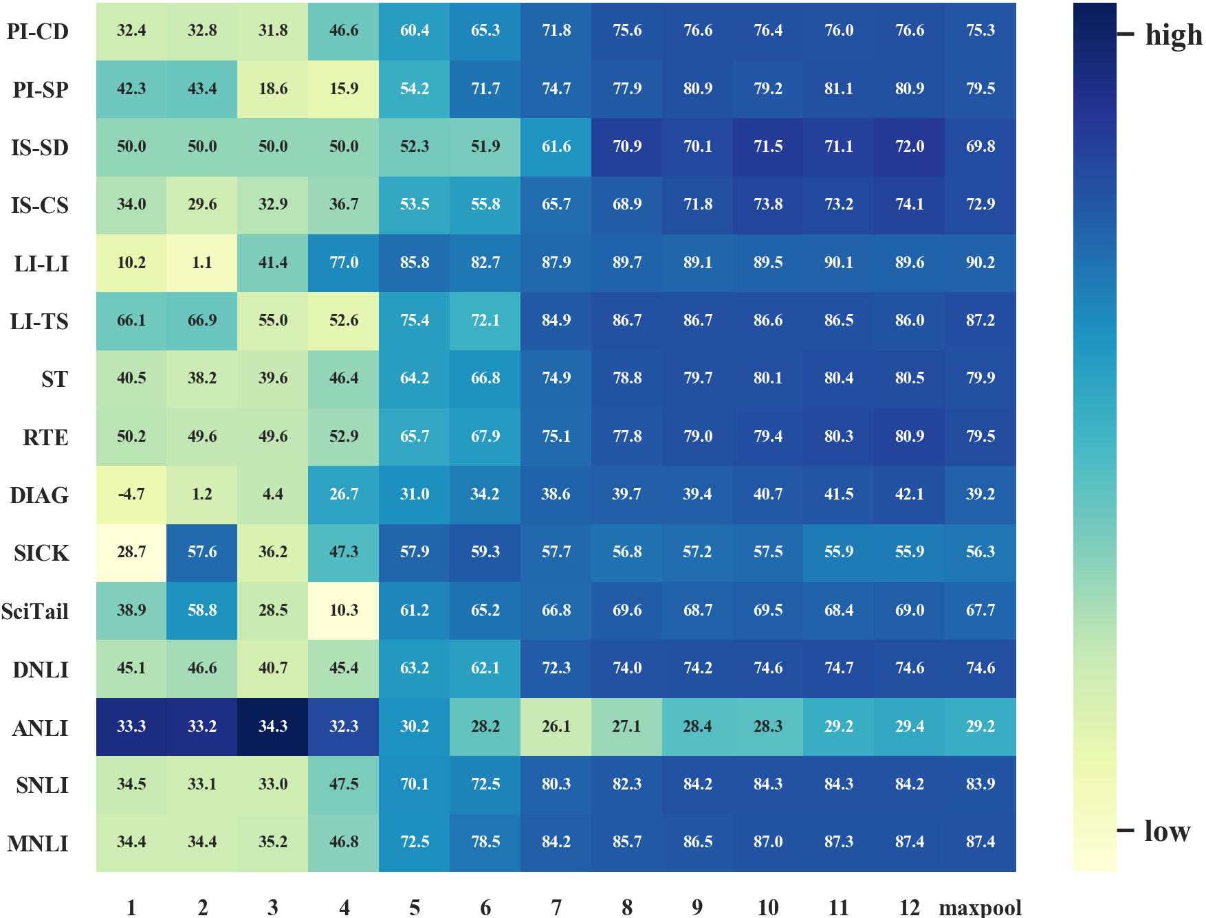
Figure 2: Per-layer analysis for RoBERTa(base) model trained on MultiNLI. Darker blue denotes higher score. ‘max’ represents the maxpooled vector across all layers. Nearly all test sets except ANLI get higher scores by using higher layers. On ANLI, the performance of the first 4 layers are close to random guess while that of higher layers is about 4 point lower than random guess.

Labels	Transformation	Datasets
($\neg$E, E)	C$\Rightarrow\neg$E, N$\Rightarrow\neg$E	IS-SD, RTE, DNLI
($\neg$C, C)	E$\Rightarrow\neg$C, N$\Rightarrow\neg$C	LI-TS
(E, C)	-	LI-LI
(N, E)	-	SciTail

Table 7: How we evaluate the test sets with only two labels in 3-way NLI classification. E,C,N,$\neg$ means entailment, contradiction, neutral and not respectively. $\Rightarrow$ means changing the left-hand side model prediction with the right-hand side label while evaluation.

6 Experimental Settings

6.1 Implementation Details

We set up both pretrained and non-pretrained model baselines for the proposed evaluation bechmarks. We rerun their public available codebases Wolf et al. (2019), including InferSent Conneau et al. (2017) (w/ and w/o Elmo Peters et al. (2018)), DAM Parikh et al. (2016) , ESIM Chen et al. (2017), BERT (uncased) Devlin et al. (2019), XLNet (cased) Yang et al. (2019) and RoBERTa Liu et al. (2019), . we map the vector at the position of the ‘[CLS]’ token in the pretrained models to three-way NLI classification via linear transformation. We show the per-layer analyses for RoBERTa model in Table 2. We try to reduce the randomness of our experiments by 3 runs using different random seeds. We report the median of the 3 runs for all the tables except the ensemble-related (Sec 5.2) experiments in Table 6. Table 7 shows how we evaluate the test sets with only two labels in 3-way NLI classification.

	RTE	SICK	SciTail	DNLI	ANLI	SNLI	MNLI
Origin	75.4	54.2	66.1	54.2	27.7	80.0	83.5
Mixed	75.5	54.3	67.3	54.8	27.4	79.9	83.4
Oracle	75.5	55.2	67.3	56.7	28.0	80.3	83.5

Table 8: The performance of BERT base model under different model selection strategies.

6.2 Model Selection Strategy

Since we test the NLI models on multiple general-purpose dataset. it is an important question how we choose the dev set. We explore 3 different model selection settings:

1) Origin: using the original in-domain dev set.

2) Mixed: using the merged dev sets which include all the instances in the in-domain and extra dev sets in generalization power tests.

3) Oracle: tuning the model for each generalization power test using its own dev set.

We show the performance of a BERT base model trained on MultiNLI utilizing the above mentioned model selection strategies in Table 8. In this paper we use the ‘origin’ mode, as it is too expensive to use the ‘oracle’ strategy in all experiments, besides we did not see much difference between the ‘mixed’ and ‘origin’ modes. Notably when we merge different training sets, we also merge their dev sets correspondingly to form a unified in-domain dev set in Table 6.

7 Related Work

Bias in NLI: The bias in the data annotation exists in many tasks, e.g. lexical inference Levy et al. (2015), visual question answering Goyal et al. (2017), ROC story cloze Cai et al. (2017); Schwartz et al. (2017) etc. The NLI models are shown to be sensitive to the compositional features in premises and hypothesesNie et al. (2019); Dasgupta et al. (2018), data permutations Schluter and Varab (2018); Wang et al. (2019c) and vulnerable to adversarial examples Iyyer et al. (2018); Minervini and Riedel (2018); Glockner et al. (2018) and crafted stress test Geiger et al. (2018); Naik et al. (2018). Other evidences of artifacts include sentence occurrence Zhang et al. (2019), syntactic heuristics between hypotheses and premises McCoy et al. (2019) and black-box clues derived from neural models Gururangan et al. (2018); Poliak et al. (2018b); He et al. (2019). Rudinger et al. (2017) showed hypotheses in SNLI has the evidence of gender, racial stereotypes, etc. Sanchez et al. (2018) analysed the behaviour of NLI models and the factors to be more robust. Feng et al. (2019) discussed how to use partial-input baseline in future dataset creation. Belinkov et al. (2019); Clark et al. (2019); He et al. (2019); Yaghoobzadeh et al. (2019); Ding et al. (2020); Utama et al. (2020a) proposed efficient methods to mitigate a particular known bias in NLI. Wu et al. (2020); Utama et al. (2020b) investigates the method to improve model generalization by debiasing unknown dataset bias in natural language understanding and question answering tasks.

Benchmark collection in NLI: GLUE Wang et al. (2019b, a) benchmark contains several NLI-related benchmark datasets. However it does not include adversarial test sets, domain specific test Romanov and Shivade (2018); Ravichander et al. (2019). Researchers create NLI datasets using different collection criteria, such as recasting other NLP tasks to NLI Poliak et al. (2018a), iteratively filtering adversarial training data by model decisions Bras et al. (2020) (model-in-the-loop), counterfactually augmenting training data by human editing examples to break the model Kaushik et al. (2020) (human-in-the-loop) and multi-round annotating depending on both human and model decisions Nie et al. (2020).

8 Conclusions

We try to investigate how to build robust and generalized NLI models by model-agnostic debiasing strategies, including mixture of experts ensemble (MoE), data augmentation (DA), dataset merging and model ensemble, and benchmark these methods on various adversarial and general purpose datasets. Our findings suggest model-level MoE ensemble, text swap DA and performance based dataset merging would effectively combat multiple (though not all) distinct biases.

Although we haven’t found a debiasing strategy that can guarantee the NLI models to be more robust on every adversarial dataset used in this paper, we leave the question of whether such a debiasing method exists for future research.

References

- Belinkov et al. (2019) Yonatan Belinkov, Adam Poliak, Stuart Shieber, Benjamin Van Durme, and Alexander Rush. 2019. On adversarial removal of hypothesis-only bias in natural language inference. pages 256–262, Minneapolis, Minnesota. Association for Computational Linguistics.
- Bird and Loper (2004) Steven Bird and Edward Loper. 2004. NLTK: The natural language toolkit. In Proceedings of the ACL Interactive Poster and Demonstration Sessions, pages 214–217, Barcelona, Spain. Association for Computational Linguistics.
- Bowman et al. (2015) Samuel R. Bowman, Gabor Angeli, Christopher Potts, and Christopher D. Manning. 2015. A large annotated corpus for learning natural language inference. In Proceedings of the 2015 Conference on Empirical Methods in Natural Language Processing, pages 632–642, Lisbon, Portugal. Association for Computational Linguistics.
- Bras et al. (2020) Ronan Le Bras, Swabha Swayamdipta, Chandra Bhagavatula, Rowan Zellers, Matthew E. Peters, Ashish Sabharwal, and Yejin Choi. 2020. Adversarial filters of dataset biases. CoRR, abs/2002.04108.
- Cai et al. (2017) Zheng Cai, Lifu Tu, and Kevin Gimpel. 2017. Pay attention to the ending:strong neural baselines for the ROC story cloze task. In Proceedings of the 55th Annual Meeting of the Association for Computational Linguistics (Volume 2: Short Papers), pages 616–622, Vancouver, Canada. Association for Computational Linguistics.
- Chen et al. (2017) Qian Chen, Xiaodan Zhu, Zhen-Hua Ling, Si Wei, Hui Jiang, and Diana Inkpen. 2017. Enhanced LSTM for natural language inference. In Proceedings of the 55th Annual Meeting of the Association for Computational Linguistics (Volume 1: Long Papers), pages 1657–1668, Vancouver, Canada. Association for Computational Linguistics.
- Clark et al. (2019) Christopher Clark, Mark Yatskar, and Luke Zettlemoyer. 2019. Don’t take the easy way out: Ensemble based methods for avoiding known dataset biases. In Proceedings of the 2019 Conference on Empirical Methods in Natural Language Processing and the 9th International Joint Conference on Natural Language Processing (EMNLP-IJCNLP), pages 4069–4082, Hong Kong, China. Association for Computational Linguistics.
- Conneau et al. (2017) Alexis Conneau, Douwe Kiela, Holger Schwenk, Loïc Barrault, and Antoine Bordes. 2017. Supervised learning of universal sentence representations from natural language inference data. In Proceedings of the 2017 Conference on Empirical Methods in Natural Language Processing, pages 670–680, Copenhagen, Denmark. Association for Computational Linguistics.
- Dagan et al. (2005) Ido Dagan, Oren Glickman, and Bernardo Magnini. 2005. The PASCAL recognising textual entailment challenge. In Machine Learning Challenges, Evaluating Predictive Uncertainty, Visual Object Classification and Recognizing Textual Entailment, First PASCAL Machine Learning Challenges Workshop, MLCW 2005, Southampton, UK, April 11-13, 2005, Revised Selected Papers, volume 3944 of Lecture Notes in Computer Science, pages 177–190. Springer.
- Dagan et al. (2013) Ido Dagan, Dan Roth, Mark Sammons, and Fabio Massimo Zanzotto. 2013. Recognizing Textual Entailment: Models and Applications. Synthesis Lectures on Human Language Technologies. Morgan & Claypool Publishers.
- Dasgupta et al. (2018) Ishita Dasgupta, Demi Guo, Andreas Stuhlmüller, Samuel Gershman, and Noah D. Goodman. 2018. Evaluating compositionality in sentence embeddings. In Proceedings of the 40th Annual Meeting of the Cognitive Science Society, CogSci 2018, Madison, WI, USA, July 25-28, 2018. cognitivesciencesociety.org.
- Devlin et al. (2019) Jacob Devlin, Ming-Wei Chang, Kenton Lee, and Kristina Toutanova. 2019. BERT: Pre-training of deep bidirectional transformers for language understanding. In Proceedings of the 2019 Conference of the North American Chapter of the Association for Computational Linguistics: Human Language Technologies, Volume 1 (Long and Short Papers), pages 4171–4186, Minneapolis, Minnesota. Association for Computational Linguistics.
- Ding et al. (2020) Xiaoan Ding, Tianyu Liu, Baobao Chang, Zhifang Sui, and Kevin Gimpel. 2020. Discriminatively-tuned generative classifiers for robust natural language inference. CoRR, abs/2010.03760.
- Feng et al. (2019) Shi Feng, Eric Wallace, and Jordan Boyd-Graber. 2019. Misleading failures of partial-input baselines. In Proceedings of the 57th Annual Meeting of the Association for Computational Linguistics, pages 5533–5538, Florence, Italy. Association for Computational Linguistics.
- Geiger et al. (2018) Atticus Geiger, Ignacio Cases, Lauri Karttunen, and Christopher Potts. 2018. Stress-testing neural models of natural language inference with multiply-quantified sentences. CoRR, abs/1810.13033.
- Glockner et al. (2018) Max Glockner, Vered Shwartz, and Yoav Goldberg. 2018. Breaking NLI systems with sentences that require simple lexical inferences. In Proceedings of the 56th Annual Meeting of the Association for Computational Linguistics (Volume 2: Short Papers), pages 650–655, Melbourne, Australia. Association for Computational Linguistics.
- Goyal et al. (2017) Yash Goyal, Tejas Khot, Douglas Summers-Stay, Dhruv Batra, and Devi Parikh. 2017. Making the V in VQA matter: Elevating the role of image understanding in visual question answering. In 2017 IEEE Conference on Computer Vision and Pattern Recognition, CVPR 2017, Honolulu, HI, USA, July 21-26, 2017, pages 6325–6334. IEEE Computer Society.
- Gururangan et al. (2018) Suchin Gururangan, Swabha Swayamdipta, Omer Levy, Roy Schwartz, Samuel Bowman, and Noah A. Smith. 2018. Annotation artifacts in natural language inference data. In Proceedings of the 2018 Conference of the North American Chapter of the Association for Computational Linguistics: Human Language Technologies, Volume 2 (Short Papers), pages 107–112, New Orleans, Louisiana. Association for Computational Linguistics.
- He et al. (2019) He He, Sheng Zha, and Haohan Wang. 2019. Unlearn dataset bias in natural language inference by fitting the residual. In Proceedings of the 2nd Workshop on Deep Learning Approaches for Low-Resource NLP (DeepLo 2019), pages 132–142, Hong Kong, China. Association for Computational Linguistics.
- Hu et al. (2019) J. Edward Hu, Huda Khayrallah, Ryan Culkin, Patrick Xia, Tongfei Chen, Matt Post, and Benjamin Van Durme. 2019. Improved lexically constrained decoding for translation and monolingual rewriting. In Proceedings of the 2019 Conference of the North American Chapter of the Association for Computational Linguistics: Human Language Technologies, Volume 1 (Long and Short Papers), pages 839–850, Minneapolis, Minnesota. Association for Computational Linguistics.
- Iyyer et al. (2018) Mohit Iyyer, John Wieting, Kevin Gimpel, and Luke Zettlemoyer. 2018. Adversarial example generation with syntactically controlled paraphrase networks. In Proceedings of the 2018 Conference of the North American Chapter of the Association for Computational Linguistics: Human Language Technologies, Volume 1 (Long Papers), pages 1875–1885, New Orleans, Louisiana. Association for Computational Linguistics.
- Kaushik et al. (2020) Divyansh Kaushik, Eduard H. Hovy, and Zachary Chase Lipton. 2020. Learning the difference that makes A difference with counterfactually-augmented data. In 8th International Conference on Learning Representations, ICLR 2020, Addis Ababa, Ethiopia, April 26-30, 2020. OpenReview.net.
- Khot et al. (2018) Tushar Khot, Ashish Sabharwal, and Peter Clark. 2018. Scitail: A textual entailment dataset from science question answering. In Proceedings of the Thirty-Second AAAI Conference on Artificial Intelligence, (AAAI-18), the 30th innovative Applications of Artificial Intelligence (IAAI-18), and the 8th AAAI Symposium on Educational Advances in Artificial Intelligence (EAAI-18), New Orleans, Louisiana, USA, February 2-7, 2018, pages 5189–5197. AAAI Press.
- Levy et al. (2015) Omer Levy, Steffen Remus, Chris Biemann, and Ido Dagan. 2015. Do supervised distributional methods really learn lexical inference relations? In Proceedings of the 2015 Conference of the North American Chapter of the Association for Computational Linguistics: Human Language Technologies, pages 970–976, Denver, Colorado. Association for Computational Linguistics.
- Liu et al. (2020) Tianyu Liu, Zheng Xin, Baobao Chang, and Zhifang Sui. 2020. HypoNLI: Exploring the artificial patterns of hypothesis-only bias in natural language inference. In Proceedings of the 12th Language Resources and Evaluation Conference, pages 6852–6860, Marseille, France. European Language Resources Association.
- Liu et al. (2019) Yinhan Liu, Myle Ott, Naman Goyal, Jingfei Du, Mandar Joshi, Danqi Chen, Omer Levy, Mike Lewis, Luke Zettlemoyer, and Veselin Stoyanov. 2019. RoBERTa: A robustly optimized BERT pretraining approach. CoRR, abs/1907.11692.
- Marelli et al. (2014) Marco Marelli, Luisa Bentivogli, Marco Baroni, Raffaella Bernardi, Stefano Menini, and Roberto Zamparelli. 2014. SemEval-2014 task 1: Evaluation of compositional distributional semantic models on full sentences through semantic relatedness and textual entailment. In Proceedings of the 8th International Workshop on Semantic Evaluation (SemEval 2014), pages 1–8, Dublin, Ireland. Association for Computational Linguistics.
- Matthews (1975) Brian W Matthews. 1975. Comparison of the predicted and observed secondary structure of t4 phage lysozyme. Biochimica et Biophysica Acta (BBA)-Protein Structure, 405(2):442–451.
- McCoy et al. (2019) Tom McCoy, Ellie Pavlick, and Tal Linzen. 2019. Right for the wrong reasons: Diagnosing syntactic heuristics in natural language inference. In Proceedings of the 57th Annual Meeting of the Association for Computational Linguistics, pages 3428–3448, Florence, Italy. Association for Computational Linguistics.
- Minervini and Riedel (2018) Pasquale Minervini and Sebastian Riedel. 2018. Adversarially regularising neural NLI models to integrate logical background knowledge. In Proceedings of the 22nd Conference on Computational Natural Language Learning, pages 65–74, Brussels, Belgium. Association for Computational Linguistics.
- Naik et al. (2018) Aakanksha Naik, Abhilasha Ravichander, Norman Sadeh, Carolyn Rose, and Graham Neubig. 2018. Stress test evaluation for natural language inference. In Proceedings of the 27th International Conference on Computational Linguistics, pages 2340–2353, Santa Fe, New Mexico, USA. Association for Computational Linguistics.
- Ng et al. (2019) Nathan Ng, Kyra Yee, Alexei Baevski, Myle Ott, Michael Auli, and Sergey Edunov. 2019. Facebook FAIR’s WMT19 news translation task submission. In Proceedings of the Fourth Conference on Machine Translation (Volume 2: Shared Task Papers, Day 1), pages 314–319, Florence, Italy. Association for Computational Linguistics.
- Nie et al. (2019) Yixin Nie, Yicheng Wang, and Mohit Bansal. 2019. Analyzing compositionality-sensitivity of NLI models. In The Thirty-Third AAAI Conference on Artificial Intelligence, AAAI 2019, The Thirty-First Innovative Applications of Artificial Intelligence Conference, IAAI 2019, The Ninth AAAI Symposium on Educational Advances in Artificial Intelligence, EAAI 2019, Honolulu, Hawaii, USA, January 27 - February 1, 2019, pages 6867–6874. AAAI Press.
- Nie et al. (2020) Yixin Nie, Adina Williams, Emily Dinan, Mohit Bansal, Jason Weston, and Douwe Kiela. 2020. Adversarial NLI: A new benchmark for natural language understanding. In Proceedings of the 58th Annual Meeting of the Association for Computational Linguistics, pages 4885–4901, Online. Association for Computational Linguistics.
- Parikh et al. (2016) Ankur Parikh, Oscar Täckström, Dipanjan Das, and Jakob Uszkoreit. 2016. A decomposable attention model for natural language inference. In Proceedings of the 2016 Conference on Empirical Methods in Natural Language Processing, pages 2249–2255, Austin, Texas. Association for Computational Linguistics.
- Pennington et al. (2014) Jeffrey Pennington, Richard Socher, and Christopher Manning. 2014. GloVe: Global vectors for word representation. In Proceedings of the 2014 Conference on Empirical Methods in Natural Language Processing (EMNLP), pages 1532–1543, Doha, Qatar. Association for Computational Linguistics.
- Peters et al. (2018) Matthew Peters, Mark Neumann, Mohit Iyyer, Matt Gardner, Christopher Clark, Kenton Lee, and Luke Zettlemoyer. 2018. Deep contextualized word representations. In Proceedings of the 2018 Conference of the North American Chapter of the Association for Computational Linguistics: Human Language Technologies, Volume 1 (Long Papers), pages 2227–2237, New Orleans, Louisiana. Association for Computational Linguistics.
- Poliak et al. (2018a) Adam Poliak, Aparajita Haldar, Rachel Rudinger, J. Edward Hu, Ellie Pavlick, Aaron Steven White, and Benjamin Van Durme. 2018a. Collecting diverse natural language inference problems for sentence representation evaluation. In Proceedings of the 2018 Conference on Empirical Methods in Natural Language Processing, pages 67–81, Brussels, Belgium. Association for Computational Linguistics.
- Poliak et al. (2018b) Adam Poliak, Jason Naradowsky, Aparajita Haldar, Rachel Rudinger, and Benjamin Van Durme. 2018b. Hypothesis only baselines in natural language inference. In Proceedings of the Seventh Joint Conference on Lexical and Computational Semantics, pages 180–191, New Orleans, Louisiana. Association for Computational Linguistics.
- Ravichander et al. (2019) Abhilasha Ravichander, Aakanksha Naik, Carolyn Rose, and Eduard Hovy. 2019. EQUATE: A benchmark evaluation framework for quantitative reasoning in natural language inference. In Proceedings of the 23rd Conference on Computational Natural Language Learning (CoNLL), pages 349–361, Hong Kong, China. Association for Computational Linguistics.
- Romanov and Shivade (2018) Alexey Romanov and Chaitanya Shivade. 2018. Lessons from natural language inference in the clinical domain. In Proceedings of the 2018 Conference on Empirical Methods in Natural Language Processing, pages 1586–1596, Brussels, Belgium. Association for Computational Linguistics.
- Rudinger et al. (2017) Rachel Rudinger, Chandler May, and Benjamin Van Durme. 2017. Social bias in elicited natural language inferences. In Proceedings of the First ACL Workshop on Ethics in Natural Language Processing, pages 74–79, Valencia, Spain. Association for Computational Linguistics.
- Sanchez et al. (2018) Ivan Sanchez, Jeff Mitchell, and Sebastian Riedel. 2018. Behavior analysis of NLI models: Uncovering the influence of three factors on robustness. In Proceedings of the 2018 Conference of the North American Chapter of the Association for Computational Linguistics: Human Language Technologies, Volume 1 (Long Papers), pages 1975–1985, New Orleans, Louisiana. Association for Computational Linguistics.
- Schluter and Varab (2018) Natalie Schluter and Daniel Varab. 2018. When data permutations are pathological: the case of neural natural language inference. In Proceedings of the 2018 Conference on Empirical Methods in Natural Language Processing, pages 4935–4939, Brussels, Belgium. Association for Computational Linguistics.
- Schwartz et al. (2017) Roy Schwartz, Maarten Sap, Ioannis Konstas, Leila Zilles, Yejin Choi, and Noah A. Smith. 2017. The effect of different writing tasks on linguistic style: A case study of the ROC story cloze task. In Proceedings of the 21st Conference on Computational Natural Language Learning (CoNLL 2017), pages 15–25, Vancouver, Canada. Association for Computational Linguistics.
- Tsuchiya (2018) Masatoshi Tsuchiya. 2018. Performance impact caused by hidden bias of training data for recognizing textual entailment. In Proceedings of the Eleventh International Conference on Language Resources and Evaluation (LREC 2018), Miyazaki, Japan. European Language Resources Association (ELRA).
- Utama et al. (2020a) Prasetya Ajie Utama, Nafise Sadat Moosavi, and Iryna Gurevych. 2020a. Mind the trade-off: Debiasing NLU models without degrading the in-distribution performance. In Proceedings of the 58th Annual Meeting of the Association for Computational Linguistics, pages 8717–8729, Online. Association for Computational Linguistics.
- Utama et al. (2020b) Prasetya Ajie Utama, Nafise Sadat Moosavi, and Iryna Gurevych. 2020b. Towards debiasing NLU models from unknown biases. CoRR, abs/2009.12303.
- Wang et al. (2019a) Alex Wang, Yada Pruksachatkun, Nikita Nangia, Amanpreet Singh, Julian Michael, Felix Hill, Omer Levy, and Samuel R. Bowman. 2019a. Superglue: A stickier benchmark for general-purpose language understanding systems. In Advances in Neural Information Processing Systems 32: Annual Conference on Neural Information Processing Systems 2019, NeurIPS 2019, 8-14 December 2019, Vancouver, BC, Canada, pages 3261–3275.
- Wang et al. (2019b) Alex Wang, Amanpreet Singh, Julian Michael, Felix Hill, Omer Levy, and Samuel R. Bowman. 2019b. GLUE: A multi-task benchmark and analysis platform for natural language understanding. In 7th International Conference on Learning Representations, ICLR 2019, New Orleans, LA, USA, May 6-9, 2019. OpenReview.net.
- Wang et al. (2019c) Haohan Wang, Da Sun, and Eric P. Xing. 2019c. What if we simply swap the two text fragments? A straightforward yet effective way to test the robustness of methods to confounding signals in nature language inference tasks. In The Thirty-Third AAAI Conference on Artificial Intelligence, AAAI 2019, The Thirty-First Innovative Applications of Artificial Intelligence Conference, IAAI 2019, The Ninth AAAI Symposium on Educational Advances in Artificial Intelligence, EAAI 2019, Honolulu, Hawaii, USA, January 27 - February 1, 2019, pages 7136–7143. AAAI Press.
- Wieting and Gimpel (2018) John Wieting and Kevin Gimpel. 2018. ParaNMT-50M: Pushing the limits of paraphrastic sentence embeddings with millions of machine translations. In Proceedings of the 56th Annual Meeting of the Association for Computational Linguistics (Volume 1: Long Papers), pages 451–462, Melbourne, Australia. Association for Computational Linguistics.
- Williams et al. (2018) Adina Williams, Nikita Nangia, and Samuel Bowman. 2018. A broad-coverage challenge corpus for sentence understanding through inference. In Proceedings of the 2018 Conference of the North American Chapter of the Association for Computational Linguistics: Human Language Technologies, Volume 1 (Long Papers), pages 1112–1122, New Orleans, Louisiana. Association for Computational Linguistics.
- Wolf et al. (2019) Thomas Wolf, Lysandre Debut, Victor Sanh, Julien Chaumond, Clement Delangue, Anthony Moi, Pierric Cistac, Tim Rault, Rémi Louf, Morgan Funtowicz, and Jamie Brew. 2019. Huggingface’s transformers: State-of-the-art natural language processing. CoRR, abs/1910.03771.
- Wu et al. (2020) Mingzhu Wu, Nafise Sadat Moosavi, Andreas Rücklé, and Iryna Gurevych. 2020. Improving QA generalization by concurrent modeling of multiple biases. CoRR, abs/2010.03338.
- Yaghoobzadeh et al. (2019) Yadollah Yaghoobzadeh, Remi Tachet des Combes, Timothy J. Hazen, and Alessandro Sordoni. 2019. Robust natural language inference models with example forgetting. CoRR, abs/1911.03861.
- Yang et al. (2019) Zhilin Yang, Zihang Dai, Yiming Yang, Jaime G. Carbonell, Ruslan Salakhutdinov, and Quoc V. Le. 2019. XLNet: Generalized autoregressive pretraining for language understanding. In Advances in Neural Information Processing Systems 32: Annual Conference on Neural Information Processing Systems 2019, NeurIPS 2019, 8-14 December 2019, Vancouver, BC, Canada, pages 5754–5764.
- Zhang et al. (2019) Guanhua Zhang, Bing Bai, Jian Liang, Kun Bai, Shiyu Chang, Mo Yu, Conghui Zhu, and Tiejun Zhao. 2019. Selection bias explorations and debias methods for natural language sentence matching datasets. In Proceedings of the 57th Annual Meeting of the Association for Computational Linguistics, pages 4418–4429, Florence, Italy. Association for Computational Linguistics.