Be It Unresolved: Measuring Time Delays from Lensed Supernovae

Abstract

Gravitationally lensed Type Ia supernovae may be the next frontier in cosmic probes, able to deliver independent constraints on dark energy, spatial curvature, and the Hubble constant. Measurements of time delays between the multiple images become more incisive due to the standardized candle nature of the source, monitoring for months rather than years, and partial immunity to microlensing. While currently extremely rare, hundreds of such systems should be detected by upcoming time domain surveys. Even more will have the images spatially unresolved, with the observed lightcurve a superposition of time delayed image fluxes. We investigate whether unresolved images can be recognized as lensed sources given only lightcurve information, and whether time delays can be extracted robustly. We develop a method that successfully identifies such systems, with a false positive rate of $\lesssim 5\%$, and measures the time delays with a completeness of $\gtrsim 93\%$ and with a bias of $\lesssim 0.5\%$ for $\Delta t_{\rm fit}\gtrsim 10$ days.

I Introduction

Gravitational lensing is the most visually striking demonstration of the curvature of spacetime. An individual source emits signals that reach the observer from different directions and at different times, forming multiple images. Moreover, these image separations and time delays carry important cosmological information on the distances and gravitational potentials along the lines of sight. For a variable source, repeated monitoring of the image flux allows estimation of the time delay, an important ingredient for the time delay distance mapping the cosmic expansion.

Time delay distances derived from monitoring quasars over years or even a decade are in use as a cosmological probe Wong et al. (2019a); Millon et al. (2020); Shajib et al. (2020); Treu and Marshall (2016). Quasars are plentiful, but their intrinsic time variability is unpredictable and it is challenging to separate out microlensing – additional time variation due to motion of objects near the lines of sights. This means that often several years ($\gtrsim 5$) of data must be accumulated before time delays can be measured with precision. With forthcoming surveys, detections of lensed Type Ia supernovae (SNe) – supernovae were the source Refsdal (1964) originally proposed for the time delay cosmography technique – will become much more numerous (only two systems have currently been published Kelly et al. (2015); Goobar et al. (2017)). These have the advantage of possessing better known time behavior (i.e. their flux vs time, or lightcurves, are more standard), with a characteristic time scale of a couple of months, enabling more rapid time delay estimation, and have a period of insensitivity to microlensing when measured in multiple wavelength filters Goldstein et al. (2018).

Supernova time delays have been put forward as ways to measure the Hubble constant (Oguri and Marshall, 2010), with application to the first lensed SN, called Refsdal, discussed in detail in Kelly et al. (2015, 2016); Rodney et al. (2016); Grillo et al. (2018); Vega-Ferrero et al. (2018). This involves cluster lensing with clearly spatially separated images. Simulation studies of lensed SN with images brightening well separated in time, i.e. time delays of $\gtrsim 60$ days, is discussed in Pierel and Rodney (2019). Here we concentrate on the opposite regime, where images are neither spatially nor temporally separated – unresolved.

Since typical galaxy lensing time delays are less than or of order the SN rise and fall time, when the images are not spatially well separated the observation is of an overlapping, summed lightcurve, offering a challenge to the time delay measurement. Indeed, one expects more lensed SNe to be unresolved than resolved. Here we take up the challenge and explore whether we can 1) recognize a SN lightcurve as being composed of multiple unresolved images, and 2) accurately measure the time delay. Due to their property of having somewhat standard lightcurve shapes, and that upcoming surveys will devote considerable resources to studying them, including through follow up observations, we focus on Type Ia supernovae; however, our fitting approach is suitable for a wide variety of transients. This focus also follows from the use of Type Ia SN as luminosity distance indicators in addition; the combination of luminosity distance and time delay distance (possibly from two different SN Ia samples) can be quite powerful for a variety of cosmological characteristics, e.g. Denissenya et al. (2018); Liao et al. (2020); Lyu et al. (2020); Pandey et al. (2020); Wong et al. (2019b); Arendse et al. (2020); Liao et al. (2019); Taubenberger et al. (2019); Collett et al. (2019); Liao et al. (2017); Treu and Marshall (2016).

In Section II we discuss the data sets expected from upcoming surveys, including the multiband lightcurve and noise properties. We introduce our lightcurve fitting method in Sec. III, and test it in several ways on mock data characteristic of upcoming surveys in Sec. IV. A summary and avenues for future development are presented in Sec. V.

II Forthcoming Supernova Datasets

High-redshift supernovae are efficiently discovered with cadenced “rolling” wide-field imaging surveys (Astier et al., 2006). Fields of view of tens of arcminutes and greater ensure that multiple SNe are active within an untargeted pointing. A cadence of several days ensures that those supernovae will be discovered, ideally early in their evolution to ensure follow-up observations. The survey telescope, instrumentation, and design define the search volume, both in terms of the monitored solid angle and the depth, which then determine the number of supernovae that can be discovered.

Gravitationally lensed SNe are relatively rare, only one in roughly a thousand SNe are expected to be strongly lensed. Only surveys that monitor a large volume over a long control time are capable of discovering interesting numbers of lensed SNe. The Zwicky Transient Facility (ZTF) (Bellm et al., 2018) and the Vera C. Rubin Observatory Legacy Survey of Space and Time (LSST) (Ivezić et al., 2019) are two surveys that will discover an interesting number of gravitationally-lensed SNe of all types.

ZTF is a three year survey and is composed of a public survey, which monitors 15,000 deg² every 3 nights to $g,r\approx 20.5$ mag, a partnership survey that adds supplemental high-cadence $g,r$ and $i$ exposures for a subset of sky, and Caltech time. The nominal LSST wide-fast-deep (WFD) 10-year survey (known as minion 1016) covers $\sim$20,000 deg² and cycles $ugrizy$ every two-three weeks to a limiting magnitude of $\sim 23.5$ mag. Goldstein et al. (2019) forecast that ZTF (LSST) can make early discoveries of 0.02 (0.79) 91bg-like, 0.17 (5.92) 91T-like, 1.22 (47.84) Type Ia, 2.76 (88.51) Type IIP, 0.31 (12.78) Type IIL, and 0.36 (15.43) Type Ib/c lensed SNe per year. They also forecast that the surveys can discover at least 3.75 (209.32) Type IIn lensed SNe per year, for a total of at least 8.60 (380.60) lensed supernovae per year under fiducial observing strategies. The simulations and resultant light curves used to make these forecasts serve as the test data used in this article. We concentrate on the ZTF simulations in this work, to get an indication of nearer term results. The method however applies equally well to LSST simulation data. See also Wojtak et al. (2019); Huber et al. (2019); Verma et al. (2019); Goldstein et al. (2018).

For lens systems with small Einstein radii, image separations of multiple images can be too small to be spatially resolved in observations. Goldstein et al. (2019) find that over half of strongly-lensed SNe discovered by LSST will have a minimum angular separation of $<1^{\prime\prime}$ and a significant fraction of those will have separations of $<0.5^{\prime\prime}$. Many strongly-lensed supernova discoveries will thus be unresolved by traditional ground-based observations. Robust determination of time delays from the single observed light curve comprised of the sum of light from multiple unresolved images could be valuable in increasing the number of lensed supernova systems usable for cosmology from upcoming surveys.

Supplemental high-resolution imaging, e.g. from adaptive optics or space observations, can deliver important information. For example, an external determination of the number of images in the lensed system, and hence the number of time delays, fixes what otherwise would be a free parameter in the fit of an unresolved light curve. However, this would likely be at a single epoch, and the monitoring telescope that delivers the lightcurve might not separate the images. Thus the technique presented here is still of use in these cases.

III Fitting an Unresolved Lightcurve

III.1 Modeling the Lightcurve

The observed unresolved lightcurve is the sum of the fluxes from each of the unresolved images, each image $i$ having the same light curve shape since it comes from the same source, but with differing amplitudes $a_{i}$ and delayed observed phases, i.e. dates of explosion $t_{i}$.

The light curve observed in the $j$th filter (we use filter and band interchangeably), summed over $N_{I}$ images, can be written as

$$F_{j}(t)=\sum_{i=1}^{N_{I}}a_{i}\,f_{j}(t-t_{i})\,,$$ (1)

where $f_{j}$ is the intrinsic light curve in the $j$th filter. As the science measurements of interest are the relative time delays and magnifications, we work in terms of the parameters $\Delta t_{i}\equiv t_{i}-t_{1}$ and $\mu_{i}\equiv a_{i}/a_{1}$ defined relative to the first, earliest image. For simplicity, one can choose $t_{1}=0$ so that Eq. (1) is

$$F_{j}(t)=\sum_{i=1}^{N_{I}}\mu_{i}\mathcal{F}_{j}(t-\Delta t_{i})\,,$$ (2)

where of course $\mu_{1}=1$ and $\Delta t_{1}=0$, and $\mathcal{F}_{j}(t)\equiv a_{1}f_{j}(t)$ is a scaled version of the source lightcurve.

Our model fits both the underlying multi-band light curve shapes, $\mathcal{F}_{j}(t)$, and the relative magnifications and time delays of each of the images. Using a fixed template for $\mathcal{F}_{j}(t)$ is unlikely to give the flexibility for fits to a diverse set of supernovae, and indeed may lead to biases on time delay estimation, so we want to keep $\mathcal{F}_{j}(t)$ adaptable. The underlying multi-band light curve shapes $\mathcal{F}_{j}(t)$ are modeled as a fiducial function with a shape that is generically similar to supernovae, modified multiplicatively by a truncated series of orthogonal functions. Specifically, we choose $\mathcal{F}_{j}(t)$ to be the product of a log-normal function multiplied by a basis expansion with respect to the first four Chebyshev functions,

$$\mathcal{F}_{j}(t) =N_{j}\,\frac{1}{t}\exp\left[-\frac{(\ln t-b_{j})^{2}}{2\sigma_{j}^{2}}\right]$$ (3)

$$\qquad\times\left[1+C_{1,j}t_{s,j}+C_{2,j}(2t_{s,j}^{2}-1)+C_{3,j}(4t_{s,j}^{3}-3t_{s,j})+C_{4,j}(8t_{s,j}^{4}-8t_{s,j}^{2}+1)\right]\;.$$

Chebyshev functions have been widely used in Crossing statistics to give the desired flexibility Shafieloo et al. (2011); Shafieloo (2012a, b); Hazra and Shafieloo (2014). The time variable in the crossing terms uses $t_{s,j}\equiv t/t_{j,{\rm max}}-1$.

In this model, the underlying light curve in a single filter is described by one normalization $N_{j}$ and six shape parameters: $b_{j}$, $\sigma_{j}$, $C_{1,j}$, $C_{2,j}$, $C_{3,j}$, $C_{4,j}$. Thus to describe light curves composed of $N_{I}$ images in $N_{B}$ bands, there are $2(N_{I}-1)+7N_{B}+1$ parameters, where there is 1 parameter for the numerical fit shift parameter $t_{1}$.

In this article we make two simplifying restrictions. We concentrate on systems with only two images (or simply one if it is unlensed, for testing). The unresolved light curve consisting of two images is given by

$$F_{j}(t)=\mathcal{F}_{j}(t)+\mu\,\mathcal{F}_{j}(t-\Delta t)\;,$$ (4)

where the light curve of the first image $\mathcal{F}_{j}(t)$ is described by Eq. (3) (together with the shift parameter $t_{1}$) and the second image by a shifted, scaled version of it. For the ZTF-like systems we have observations in $g,r,i$ filters. Therefore, we have $2+7\times 3+1=24$ fit parameters, two of which are the parameters of cosmological interest, namely the relative time delay $\Delta t$ between the images and their relative magnification $\mu$. The second simplification is that here we do not include the effect of microlensing on the light curve (nor do the simulations we use from Goldstein et al. (2019)). Microlensing can introduce generally small, slowly changing magnifications that are different for each image, though correlated for the different filters of the same image. (Indeed, Goldstein et al. (2019) have shown that the color, i.e. differences between filters, is insensitive to microlensing for much of the phase relevant to time delay estimation.) For the small image separations we consider here for unresolved lensed SN, microlensing effects between images may also be reduced. Nevertheless, expanding our model to include further multiplicity of images and microlensing is planned for future work.

III.2 Sampling and setting the priors

We employ Hamiltonian Monte Carlo (HMC) for sampling, since it is well suited for dealing with a few dozen parameters. Specifically, we use the PyStan package Stan Development Team (2017), a python interface to STAN Carpenter et al. (2017). We set priors on the parameters as described below, balancing broadness of the priors with convergence efficiency. As priors tend to involve the astrophysics of the source, their specific values need to be adjusted depending on the type of transient. Here we focus on normal Type Ia supernovae. Apart from the specific priors, however, the method described in the main text should be broadly applicable to many unresolved lensed transients.

III.2.1 Prior on time delay and magnification

For time delays that are shorter than the characteristic source lightcurve width, the observed lightcurve of the combined images will tend to have one consolidated peak, while for longer time delays two separate peaks, one for each of the images, may be evident (depending on the magnification ratio). Long time delays and large magnification ratios would tend to give larger angular separation also, leading to resolved rather than unresolved lensed supernovae. However, we will apply our method to a wide range of time delays, though we concentrate on the more difficult, lower end of the range, $\Delta t\lesssim 30$. Examples of mock observed lightcurves of lensed supernovae are given in Fig. 1.

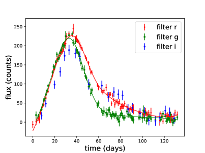
(a)  System No=51127319, $\Delta t=15.58$ days

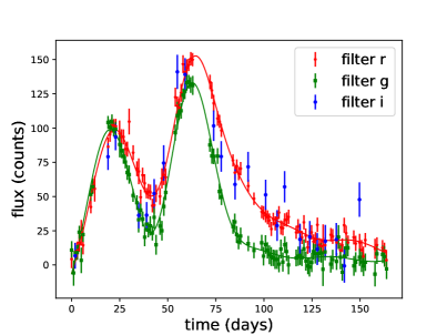
(b)  System No=40221141, $\Delta t=42.10$ days

Figure 1: Mock observations with ZTF characteristics are shown from the compilation of simulated Type-1a SNe Goldstein et al. (2019) in $g$, $r$, $i$ filters. Solid curves show a smoothing of the data, helpful for identifying the number of peaks by eye. The left panel, having a smaller time delay, shows a single peak, while the right panel with a longer time delay shows two peaks corresponding to the two images. We do not use $i$ band data for determining the number of peaks due to its generally poorer data quality and longer decline time.

As seen in Fig. 1, when the peaks are well separated one can roughly estimate the time delay from the peak positions and the relative magnification from the ratio of the peaks. These estimations can be used to set tighter priors for these large time delay systems. Conversely, when there is no evident double peak structure (in the filters we use), this imposes an upper limit on the time delay, based on the width of the peak. These features can be helpful in setting the priors on $\Delta t$ (and $\mu$ in some cases) so that the fit converges faster and we ameliorate issues of nonconvergence, or degenerate or catastrophically false fits.

The procedure begins by identifying the peaks in the smoothed light curve data (this is solely for identifying the number of peaks; the full data is used in the fit). After testing different smoothing methods we use the iterative smoothing algorithm with exponential kernel in Shafieloo et al. (2006) (see also, Shafieloo (2007); Shafieloo and Clarkson (2010); Shafieloo (2012a); Aghamousa and Shafieloo (2015)), with a smoothing scale of $12$ days. While searching for peaks, to eliminate false peaks due to noise we set a minimum height of the peaks relative to the tallest peak, minimum width, and minimum separation between peaks (details below).

• If $1$ peak identified: the time delay is not very high and we set a prior $0\leq\Delta t\leq 30$. We use a wide prior range on the relative magnification: $0\leq\mu\leq 4$. However, if the peak width is found to be very large, more than $20$ days width at 80% of peak height, we adjust the prior ranges on the time delay and relative magnification – see Appendix A for details.

• If 2 peaks identified: the time delay is high, and we can crudely estimate it as roughly the difference in the peak positions in time, say $\delta t$. Also we have an estimation for the relative magnification, roughly the ratio of the two peak heights, say $r$. We then use the following priors: $(\delta t-15)\leq\Delta t\leq(\delta t+15)$ and $r/2\leq\mu\leq 1.5r$.

• If more than 2 peaks identified: we consider the two most prominent peaks and follow the treatment above. Future work will deal with greater than two image systems.

We follow the above steps for $g$, $r$ filters separately. If one filter has one peak while the other has two or more, we follow the two peak procedure if the separation between the identified peaks of the two peak filter is less than 30 days, otherwise we follow the one peak procedure. (The logic is that for long true time delays, we would see two peaks in both filters; this step removes the spurious fitting of a noise fluctuation far on the tail of the lightcurve as a second peak.) We tested this algorithm extensively as described in Sec. IV.

III.2.2 Priors on hyper-parameters

The priors on the hyper-parameters are given in Table 1. The fit generally prefers the hyper-parameters to be somewhere in the middle of the prior ranges, e.g. $m_{j}\sim 3.5$ and $\sigma_{j}\sim 0.6$. See Appendix A for further details, as well as Sec. IV.6 for when some of the nonphysical hyper-parameter priors may be informative. In practice we treat the normalization more subtly than the hyperparameter $N_{j}$, breaking out a scaling based on the maximum flux observed and then a zeroth order basis function $C_{0,j}$; see Appendix B for details and Table 1 for the prior on $C_{0,j}$.

Hyperparameter	Prior
$\sigma_{j}$	[0.4, 0.8]
$b_{j}$	[3.0, 4.1]
$C_{0,j}$	[0.4, 2]
$C_{k,j}$	$[-5,\,5]$
$t_{1}$	$[-5,\,5]$

Table 1: Priors on the fit hyperparameters. Here $C_{k,j}$ is for $k=1,2,3,4$.

In the fits we use STAN Carpenter et al. (2017); Stan Development Team (2017) to run Hamiltonian Monte Carlo (HMC) with $7$ chains, each with $6000$ iterations and $1000$ warm up steps. We check the convergence of the chains by ensuring that the Gelman and Rubin (1992) convergence diagnostic parameter $\hat{R}<1.05$ as suggested by the STAN development team Carpenter et al. (2017).

IV Results from Testing and Validation

Using simulated data we apply the method proposed in Sec. III in four ways to test the results obtained for time delays.

1. Systematic approach: We analyze systems scanning through various values for the time delays, relative image magnifications, and noise levels, and find in what portion of this parameter space the method succeeds. These lightcurves are generated using the Hsiao template (Hsiao et al., 2007) with no microlensing, and observing conditions matched to those of Goldstein et al. (2019). We refer to this simulation tool based on the SNCosmo python package Barbary (2014) as ‘LCSimulator’ throughout this article.

2. Blind test: One author used LCsimulator to generate a set of unresolved lensed SN light curves with a variety of data properties, including several unlensed systems, and provided only the final summed lightcurve data to another author to be fit. This enables robust testing, as well as assessing false positives.

3. Applied test: More sophisticated lensed SN light curve simulations from Goldstein et al. (2019) (“the Goldstein set”) with less tightly controlled noise properties are used to assess the fitting method.

4. Validation: Once the method is finalized we return to untested systems from the Goldstein simulated data set with even less tightly controlled noise properties and fit the unresolved lensed lightcurves.

IV.1 Systematic Studies

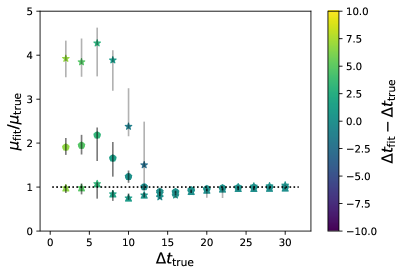
Figure 2: Noise level $=0.5\%$ (Set 1): We show $\Delta t_{\rm fit}$ (left panel) and $\mu_{\rm fit}/\mu_{\rm true}$ (right panel) vs $\Delta t_{\rm true}$. We obtain faithful results for fits giving time delays more than $\Delta t_{\rm fit}=10$ days (dashed red horizontal line in the left panel). Stars, circles, and triangles represent $\mu_{\rm true}=0.5,1,2$ respectively, while color represents $\mu_{\rm fit}/\mu_{\rm true}$ (left panel) and $\Delta t_{\rm fit}-\Delta t_{\rm true}$ (right panel). The errorbars are $95\%$ quantile around the median.

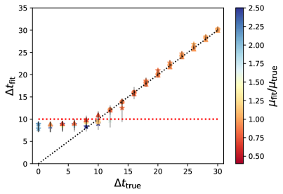
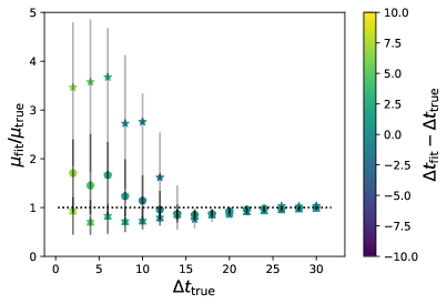
Figure 3: As Fig. 2, but for noise level $=2.5\%$ (Set 2).

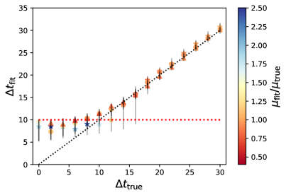
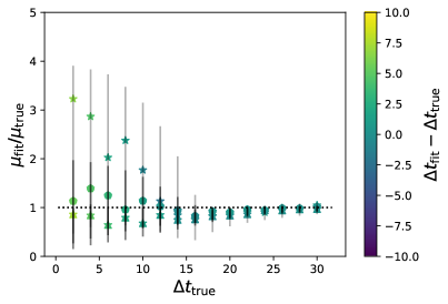
Figure 4: As Fig. 2, but for noise level $=5\%$ (Set 3).

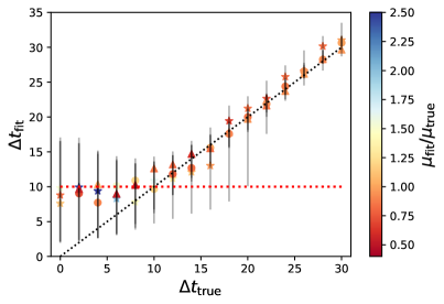
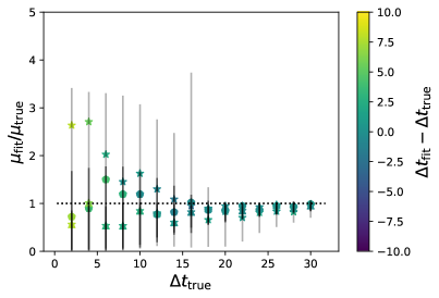
Figure 5: As Fig. 2, but for noise level $=10\%$ (Set 4).

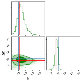
(a) $\ \mu_{\rm true}=0.5$

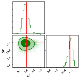
(b) $\ \mu_{\rm true}=1.0$

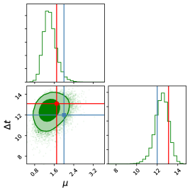
(c) $\ \mu_{\rm true}=2.0$

Figure 6: Corner plot showing the 2D joint probability distribution, and 1D PDFs, for $\Delta t$ and $\mu$, marginalizing over all other parameters. This example is for noise level $=5.0\%$ (Set 3), with $\Delta t_{\rm true}=12$ days, and three different relative magnifications: $\mu_{\rm true}=0.5,1.0,2.0$. The blue crosshairs and points show the simulation input values while the red ones show our best-fit values.

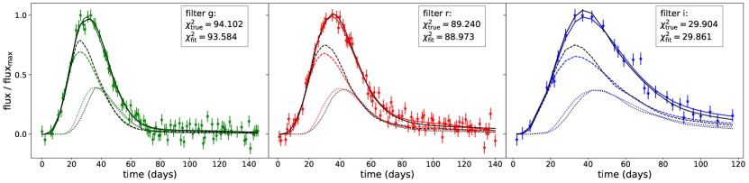
(a) $\ \mu_{\rm true}=0.5$

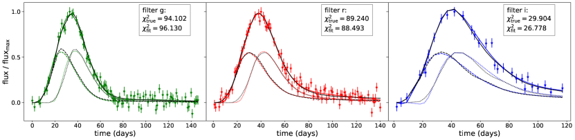
(b) $\ \mu_{\rm true}=1.0$

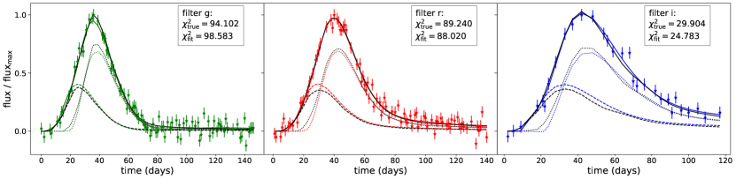
(c) $\ \mu_{\rm true}=2.0$

Figure 7: Simulated data with error bars (noise level $=5.0\%$, Set 3) is shown for a system with $\Delta t_{\rm true}=12$ days. The columns show $g$, $r$, $i$ bands and the rows show three different relative magnifications for the images: $\mu_{\rm true}=0.5,1.0,2.0$ (top, middle, bottom panels respectively). The black curves are the true light curves: dashed and dotted, and solid black curves represent the true light curves of the first and second images, and their combination. The colored curves are our equivalent reconstructions in each filter using the best fit parameters. While the key science quantity is merely the time delay, we do fit well the entire light curve, even for this moderately low time delay $\Delta t_{\rm true}=12$ days, for all the three magnifications. This is quantified through the $\chi^{2}$ values listed for the true and the reconstructed curves.

In this section we study a number of two-image systems simulated with properties scanning through time delay, relative magnification, and noise. We consider time delays $\Delta t=0,2,4,6,....,28,30$; i.e. a total of $16$ time delays. For each time delay, we simulate three systems having $\mu=0.5,1,2$. Therefore, we have $16\times 3=48$ systems in a set. We then simulate 4 such sets with different noise levels: $0.5\%,~{}2.5\%,~{}5\%$ and $10\%$ of the maximum flux. The main goal of this exercise is to test how our method performs in different conditions, finding the range of validity in terms of the time delay, magnification, and noise level (or alternately, “testing to destruction”). Set 1 has an extremely small noise level, quite unrealistic, and serves to establish fundamental limits in the method. Set 4 has an extremely large noise level, where we expect large uncertainty in our estimations. Note that each set has $48$ systems out of which $3$ are truly unlensed with $\Delta t=0$ (and several others have time delays less than some surveys’ cadence).

The summary of the results are shown in Figures 2, 3, 4, 5 for the 4 sets (each with a different noise level). Each plot has 48 systems. The three markers, ‘star’, ‘filled circle’, ‘triangle’, represent $\mu_{\rm true}=0.5,1,2$ respectively. The errorbars shown here (and throughout this paper) are discussed in Sec. IV.6. The colourbars represent the quantities $(\mu_{\rm fit}/\mu_{\rm true})$ in the left panels and $\Delta t_{\rm fit}-\Delta t_{\rm true}$ in the right panels. Note that for unlensed systems we have both $\Delta t_{\rm true}=0$, $\mu_{\rm true}=0$; so we set arbitrarily the colour according to $\mu_{\rm fit}$ for such systems and mark them by stars in the left panels; all systems with $\mu_{\rm fit}/\mu_{\rm true}>2.5$ (basically bad fits for $\mu$) have been marked with the dark blue colour for $\mu_{\rm fit}/\mu_{\rm true}=2.5$. The black dotted diagonals in the left panels of the figures represent $\Delta t_{\rm fit}=\Delta t_{\rm true}$ while the horizontal red dotted line is $\Delta t_{\rm fit}=10$ days below which the solutions depart from this relation. We quantify this further in Sec. IV.6.

From these plots we observe the following:

• For all four sets, we recover the true solutions well when $\Delta t_{\rm true}>10$ days. While the cosmology focus is on $\Delta t_{\rm fit}$, we can also find $\mu_{\rm fit}$ reasonably well. This is fairly robust with noise level, although the 10% level is noticeably more uncertain. Figure 6 shows an example of the 2D joint posterior, and 1D PDFs, for $\Delta t$ and $\mu$.

• Furthermore, although again it is not the focus for cosmology, the individual image light curves match well with the true ones. Figure 7 presents an example of the image lightcurves, as well as the unresolved total lightcurve, compared to the inputs and data.

• For $\Delta t_{\rm true}<10$ days, in all four sets $\Delta t_{\rm fit}$ does not trace $\Delta t_{\rm true}$. Instead of following the true time delay, the estimated time delay remains stable around $\Delta t_{\rm fit}\lesssim 10$ days for $\Delta t_{\rm true}<10$ days. This holds as well for a completely different intrinsic lightcurve approach not discussed in this paper, and seems likely to be due to the data sampling cadence.

The bottom line is that for unresolved lensed SN with $\Delta t_{\rm true}\geq 10$ days our method can 1) identify them as lensed, 2) fit the time delay used for cosmology, and 3) further fit the magnification and individual lightcurve shapes, not essential for cosmology. When the fit points to $\Delta t_{\rm fit}<10$ days, we do not have confidence from this approach that the SN is actually lensed or its exact time delay.

IV.2 Systematic Studies for Unlensed Systems

In the systematic study presented in the previous section, we studied a total of $12$ unlensed systems (having $\Delta t_{\rm true}=0$ and/or $\mu_{\rm true}=0$), 3 cases in each of the 4 sets. In all the $12$ unlensed cases, our fit estimates $\Delta t_{\rm fit}<10$ days and hence we would not claim detection of a lensed SN.

To investigate further, we study next a large number of unlensed systems, again simulated using LCsimulator. We consider 360 unlensed SN, 120 in each of 3 sets, with noise levels at $2.5\%$, $5\%$, $10\%$ (of the maximum of the light curve). If we use our acceptance criterion $\Delta t_{\rm fit}>10$ days suggested by Figs. 3–5 then we have no false positives for the 2.5% noise level and about 8% false positives for the 5% and 10% noise levels. However, raising the acceptance to $\Delta t_{\rm fit}>12$ days completely eliminates false positives: none out of the 360 would be mistakenly interpreted as unresolved lensed SN.

IV.3 Blind Testing

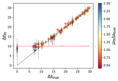
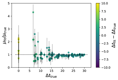
Figure 8: Blind test: As Fig. 2, but for a blind set having $100$ systems, 9 of them are unlensed while the time delays of the rest are distributed over $6-30$ days. Stars and circles represent systems with $\mu_{\rm true}\leq 1$ and $\mu_{\rm true}>1$ respectively.

To test the robustness of the developed analysis pipeline, one author simulated a set of unresolved SN light curves based on the Hsiao template (Hsiao et al., 2007), with no microlensing, and observing conditions matched to those of Goldstein et al. (2019). This set included a range of time delays, and also unlensed cases. Another author received only the final summed lightcurve data to carry out a fit, without further communication. This enabled testing without any case by case tweaking using knowledge that would be not be available for real data; in addition it served as a further test of false positives.

This test used $100$ systems with the noise level randomly set between $2.5\%$ and $10\%$ (of the maxima of the observed light curve). After the analysis was complete and fits frozen, it was revealed that $9$ systems were unlensed and the remainder had time delays distributed over $6$–$30$ days. Results are shown in Fig. 8 and appear well in line with previous tests – good tracing of the true time delay and no false negatives.

IV.4 Applied Tests on the Goldstein Set

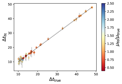
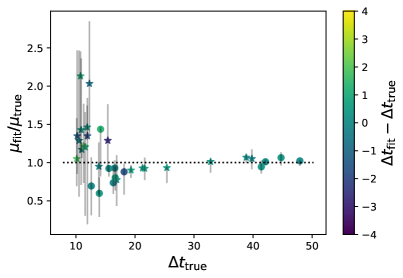
Figure 9: The best-fit time delays for 33 ZTF-like systems from Goldstein et al. (2019) are shown with respect to the true values. The colourbars show $\mu_{\rm fit}/\mu_{\rm true}$ and $\Delta t_{\rm fit}-\Delta t_{\rm true}$ in the left and the right panel respectively. Stars and filled circles represent systems with $\mu_{\rm true}\leq 1$ and $\mu_{\rm true}>1$ respectively. The figure shows that we get excellent fits and smaller errorbars for higher time delay systems.

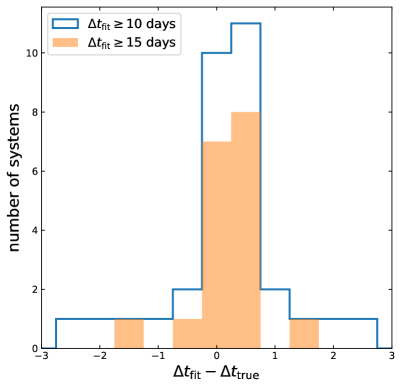
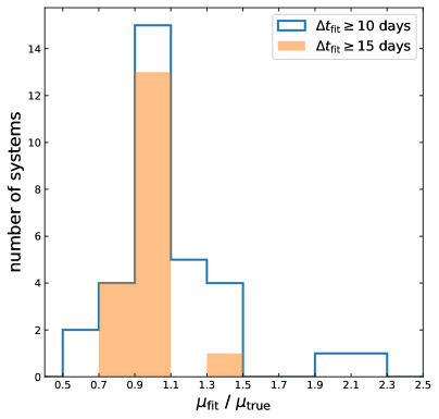
Figure 10: The histograms of the best-fit values of time delay and magnification from the set of 33 ZTF-like systems are shown relative to the true values, in bins of width 0.5 days in $\Delta t$ and 0.2 in $\mu$. The blue histogram in either panel consists of systems which we could fit with confidence, i.e. for which $\Delta t_{\rm fit}\geq 10$ ($32$ systems), with the orange shaded regions restricted to those systems with $\Delta t_{\rm fit}\geq 15$ days ($18$ systems). Note only two out of the $33$ systems in this set have $|\Delta t_{\rm fit}-\Delta t_{\rm true}|>2$ days and none have $|\Delta t_{\rm fit}-\Delta t_{\rm true}|>3$. We see that for most systems the fits are quite close to the true value.

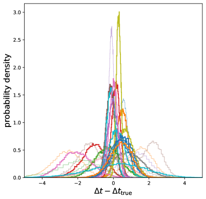
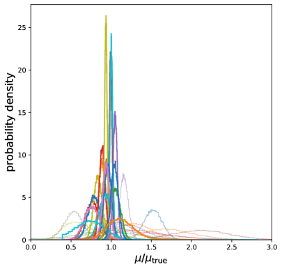
Figure 11: Rather than merely the best fit values, here we show the full 1D probability densities (PDF) of time delay and magnification (relative to the true values) of the 33 systems, plotted simultaneously. Again the full 1D histograms trace the true values quite well. Bolder curves denote systems with $\Delta t_{\rm fit}>15$ days.

For more sophisticated lensed SN simulations we employ the ZTF-Ia lensed SN simulations compiled in Goldstein et al. (2019) that fulfill the following criteria: 1) Light curve visually appears smooth (and the shape is ‘like a light curve’); 2) The system has a minimum of $200$ data points when combining $g$, $r$, $i$ bands (typically the $i$-band data points are much fewer than for the $g$, $r$ bands) and $0.5\leq\mu\equiv\mu_{2}/\mu_{1}\leq 2$, $\Delta t_{\rm true}\geq 10$ days. This gives rise to an initial set of 33 systems, with an average noise level of $\sim 7\%$.

Our results for the time delays and magnifications appear in Fig. 9. Again, the fits trace the true values. Note 7 of the 33 systems are at higher time delays than we have previously considered and the fit continues to work well (unsurprisingly since the time delays are higher, but still useful to check). Figure 10 compiles the statistics of the fits by presenting the histograms of scatter of the best fit from the true values, for the outcomes where we accept the fit results – either $\Delta t_{\rm fit}>10$ or $15$ days. The histograms are highly peaked near the true values, only $2$ of $33$ cases are off by more than 2 days in the time delay, and none by more than 3 days.

Since more information is present in the full fit distributions, not just the best fit values, Fig. 11 presents the full 1D PDFs for the time delays and magnifications. They appear fairly Gaussian and the ensemble is well peaked near the true values.

IV.5 Validation Tests on the Goldstein Set

Finally, following the previous full program of testing we apply the method to a larger sample from Goldstein et al. (2019). We consider systems with relaxed constraints on the relative magnification: $1/3\leq\mu_{\rm true}\leq 3$ while keeping the time delay range the same as the training set, $10\leq\Delta t_{\rm true}\leq 50$ days. The other criteria pertaining to the data quality are kept the same except that for the purpose of validation, we extend the testing by including noisier systems. The set of $71$ systems so identified has a larger overall noise level ($\sim 10.4\%$) compared to the previous samples so together with the relaxed constraints we therefore expect larger uncertainties and scatter.

Figure 12 shows the results for the time delays and magnifications. The method holds, though on this set it gives a larger fraction of systems not accepted as having confident detection of unresolved lensing ($\Delta t_{\rm fit}<10$ days).

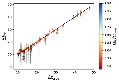
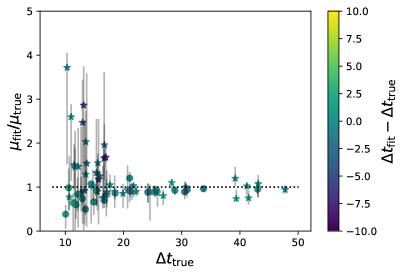
Figure 12: As Fig. 9 but for the noisier, validation set consisting of $71$ ZTF-like systems from Goldstein et al. (2019). Both panels again show fits matching the true values. Uncertainties are somewhat larger compared to Fig. 9 due to a higher overall noise level in this set.

Combining together the Goldstein sets of 33+71 lensed SN, Figure 13 presents histograms of scatter of the best fit from the true values, again for the outcomes where we accept the fit results – either $\Delta t_{\rm fit}>10$ or 15 days. The histograms remain well peaked near the true values, though with increased scatter from the increased noise.

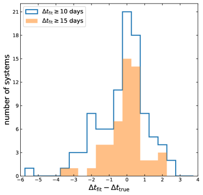
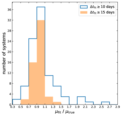
Figure 13: As Fig. 10 but for the consolidated set consisting of $33+71=104$ ZTF-like systems from Goldstein et al. (2019). Note that $97$ systems satisfy the condition $\Delta t_{\rm fit}\geq 10$ days that corresponds to the blue histogram in either of the panels whereas the orange histograms enclose $54$ systems. Again we find that for most of the systems our fit estimations are close to the respective true values.

IV.6 Assessing Precision and Accuracy

An important aspect of the use of lensed SN for cosmology is quantifying the fit precision and accuracy. We assess these below for the unresolved lensed SN we have studied.

For the fit precision, i.e. the uncertainty on the estimation, we investigate the cumulative pull distribution from the sampling chains, shown in Fig. 14. By examining the amount of probability between the 16%–84% quantiles, we find that the chains are underestimating the $\Delta t_{\rm fit}$ uncertainties by approximately a factor of $0.71$ for the systems with $\Delta t_{\rm fit}\geq 10$ (and $0.87$ for $\Delta t_{\rm fit}\geq 15$ days). This is not uncommon for flexible model spaces where the full parameter space is not thoroughly sampled. Indeed, as mentioned in Sec. III.2.2 some of the priors on the non-physical hyper-parameters are informative, i.e. running into the boundary (and extending the boundary lowers the code efficiency and convergence). Thus the details of the derived probability distribution functions (PDFs), including potentially for the time delays and magnifications, can be affected. However, this does not seem to be the case for the best fit values, as seen in the accuracy tests below. Methods for improving uncertainty quantification are being developed in further work, but in this article we will not use the uncertainties quantitatively. We can still assess the accuracy of the method for best fits however.

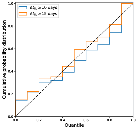
Figure 14: Cumulative probability distribution from the consolidated set consisting of $33+71=104$ ZTF-like systems from Goldstein et al. (2019). The histograms basically show the fraction of the systems for which the true time delay falls within a given probability quantile of the fit distribution. Significant deviations from the diagonal dashed line indicate under- or over-estimation of the uncertainty. The amount of probability between the $16\%$–$84\%$ percentiles is found to be $48.5\%$ for the systems with $\Delta t_{\rm fit}\geq 10$ days (blue curve), and $59.3\%$ for the systems with $\Delta t_{\rm fit}\geq 15$ days (orange curve). Therefore, we find that the uncertainty in the estimated time delay, $\sigma(\Delta t_{\rm fit})$, is underestimated by a factor of about $0.71$ for the blue curve and $0.87$ for the orange curve. This can be due in part to insufficient statistics, i.e. only 97 (54) systems in the blue (orange) histogram.

For the fit accuracy, we want to ensure this in two respects. The first is a low fraction of false positives: cases that are fit as unresolved lensed SN even though in reality they are single unlensed images. The second is bias in the time delay measurement: are estimates statistically scattered about the truth or are they systematically offset low or high.

The false positive rate was estimated by running 360 unlensed SNe in Sec. IV.2 in addition to the 12 in Sec. IV.1, as well as including unlensed SNe in the blind data set in Sec. IV.3, and considering what fraction of their fits have spurious time delay measurements inconsistent with zero delay. From the results in those subsections, the fraction of false positives can be estimated as $\lesssim 5\%$ (19 out of 381), mostly due to the higher noise levels, if we use $\Delta t_{\rm fit}>10$ days, but 0 out of 381 for $\Delta t_{\rm fit}>12$ days.

The second type of accuracy is bias. To assess bias, we compare the ensemble of fit time delays to the true inputs through Liao et al. (2015); Hojjati and Linder (2014)

$$A=\frac{1}{N_{\rm fit}}\sum\frac{\Delta t_{\rm fit}-\Delta t_{\rm true}}{\Delta t_{\rm true}}\,.$$ (5)

Note that this uses the best fit and does not involve the fit uncertainty. Fits that scatter positive and negative about the truth for the time delay do not bias cosmology estimation; only a systematic offset relative to truth shifts the cosmology.

Figure 15 shows the accuracy as a function of which fits we accept. Nominally, from previous sections, we have confidence in results with $\Delta t_{\rm fit}\geq 10$ days, i.e. $\Delta t_{\rm fit,min}=10$ days. We study the results as a function of $\Delta t_{\rm fit,min}$, finding that as soon as we move away from the boundary of 10 days, where slight variations in fit can cause the best fit to move above or below $\Delta t_{\rm fit,min}$ despite much of the probability distribution remaining below, the accuracy ranges mostly over the 0.3%–0.5% level. For cosmology use with a rather advanced data set with small statistical uncertainty, Hojjati and Linder (2014) derived a 0.2% accuracy requirement – that was for lens systems giving 1% distance measurements in each of six lens redshift bins from $z_{\rm lens}=0.1\text{--}0.6$ (see also Aghamousa and Shafieloo (2015, 2017)). Since that is rather ambitious for unresolved lensed SNe alone, we regard $\sim 0.5\%$ accuracy as quite good enough to start.

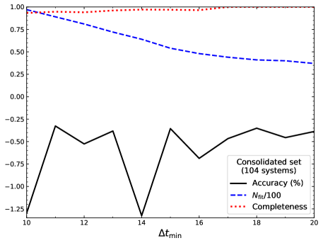
Figure 15: The accuracy $A$, Eq. (5), important for using time delays as a robust cosmological probe, is plotted vs ${\Delta t}_{\rm min}$, where only systems with $\Delta t_{\rm fit}\geq{\Delta t}_{\rm min}$ are accepted as unresolved lensed SN. The accuracy mostly lies around 0.3%–0.5%. For limited numbers of systems in the sample, deviations in one or two systems can impact the accuracy; the number of accepted systems is shown by the dashed blue curve $N_{\rm fit}/100$. The completeness, i.e. the fraction of systems that should have been accepted given a perfect fit, and were accepted as robust unresolved lens SN, is shown by the dotted red curve.

One might also consider false negatives, where the fit considers multiple images as one unlensed source. We will mostly address this in future work where we fit for the number of images, e.g. does the algorithm accurately identify the number of components. Here we simply mention that for systems with true time delays more than ten days, there are zero cases where the time delay fit is consistent with zero delay, i.e. no lensing. We can also quantify the completeness, i.e. how many systems did we have sufficient confidence in the fit to include in the results. We quantify this by taking the the total number with $\Delta t_{\rm true}\geq\Delta t_{\rm min}$ and asking how many of these did we get any fit for (i.e. $\Delta t_{\rm fit}>10$ days). The completeness is shown as the dotted red curve in Fig. 15 and ranges from 93% at $\Delta t_{\rm min}=10$ days to 97% at $\Delta t_{\rm min}=14$ days and 100% at $\Delta t_{\rm min}=17$ days.

V Conclusions

Strong gravitational lensing allows us to see a source in different positions and at different times, and so can serve as an important cosmological probe. Lensed SN have advantages over lensed quasars in having a better understood intrinsic light curve with a characteristic time scale of order a month, allowing time delay estimation after months rather than many years of monitoring. Surveys underway, such as ZTF, and forthcoming, such as ZTF-2 and LSST, will greatly increase the number of lensed SN detected. However, if the time delay is of order or shorter than the characteristic SN timescale, i.e. about a month, then the lensed nature may not be obvious either from the observed lightcurve (a superposition of the image lightcurves) or spatially resolved on the sky.

Here we investigate these unresolved lensed SN, and put forward a method for robustly extracting the time delays (and image magnifications). The time delays are directly related to the time delay distance of the supernova, adding a highly complementary cosmological probe to standard luminosity distance measurements. Knowledge of the magnifications provides important constraints on the lens modeling, needed as well. Once a transient is identified as a lensed supernova, additional resources such as high resolution imaging from ground based adaptive optics systems or space based telescopes can target it to resolve images spatially.

Our method, involving an orthogonal basis expansion around a trial lightcurve, sampled over many parameters for each band and image through Hamiltonian Monte Carlo, shows great promise. We recover the time delays (and magnifications) accurately down to $\Delta t_{\rm fit}\gtrsim 10$ days for sampling cadence and noise levels representative of ZTF and LSST surveys. The false positive rate (interpreting an unlensed SN as a lensed one) is below 5%, and the completeness (finding actually lensed SN as lensed) is 93% or better. Time delay measurement can accurately control bias to $\sim 0.5\%$.

We emphasize that the fundamentals of this technique are broadly applicable and do not rely fundamentally on SN properties. The method can be used for any transient lightcurve, with proper adjustment of hyperparameter priors. We have not yet tried this. Hamiltonian Monte Carlo provides a potentially robust sampling technique for the multidimensional parameter space necessary; our particular cases allowed 24 parameters but there is no innate limit.

Significant further developments can be made. Our future work will include fitting for the number of images as part of the process (here we did only 1 vs 2, i.e. unlensed vs two lensed images), increasing flexibility in the template plus basis expansion approach, accounting for microlensing, and establishing cadence, noise, or other requirements to push the minimum time delay for which we have confidence in the results into the regime $\Delta t_{\rm fit}<10$ days. And of course we greatly look forward to applying the method to real data from surveys and discovering a significant sample of unlensed SN.

Appendix A Hyperparameter and time delay priors

The priors on the intrinsic lightcurve parameters, the hyperparameters, are presented in Table 1. Here we give some more detail. We again caution that priors tend to involve the astrophysics of the source, and their specific values need to be adjusted depending on the type of transient. Here we focus on normal Type Ia supernovae. Apart from the specific priors, however, the method described in the main text should be broadly applicable to many unresolved lensed transients.

The parameter $b_{j}$ (known as the scale parameter in lognormal distributions) is a logarithmic time variable that gives the median of the distribution. Since a SN falls more slowly than it rises, and it peaks about 20 days after explosion, the median is around 30 days. This translates to $b_{j}\approx 3.4$. Less than 20 days or longer than 60 days (e.g. for the longer wavelength bands) seem to be unuseful parts of the parameter space, so we adopt $b_{j}\in[3.0,4.1]$. In the fits to the data, we find $b_{j}\approx 3.4$ and none of the fits approach closely the prior bounds.

The parameter $\sigma_{j}$ (known as the shape parameter) relates to the (logarithmic) width of the distribution and interacts with $b_{j}$ to give skewness, shifting the mode (and mean) from the median. In particular the mode, i.e. maximum flux, occurs at $\exp(b_{j}-\sigma_{j}^{2})$. If the median is 30 days and the mode is at 20 days after explosion, then $\sigma_{j}\approx 0.64$. Extending the maximum all the way to 30 days after explosion would still give $\sigma_{j}<0.8$ for the largest $b_{j}$, i.e. the latest median. For the maximum no earlier than 17 days after explosion, one gets $\sigma_{j}>0.4$ for the smallest $b_{j}$. Thus the range adopted is $\sigma_{j}\in[0.4,0.8]$. In the fits to the data, we find $\mu\approx 0.64$ and none of the fits approach closely the prior bounds.

Note these priors are specific to normal Type Ia supernovae we would use for cosmology. They are motivated by the lognormal template, which will be further modified by the basis expansion terms. However, they work well in practice. For other supernovae, or other transients, the priors would need to be adjusted although the fitting method should still be substantially unchanged.

The fit shift parameter $t_{1}$ comes from numerics using noisy data, not the astrophysics of supernovae. For low flux, photon noise and photometry scatter are especially influential, and the explosion time can be misestimated. Introducing $t_{1}$ helps mitigate this as the fit can be shifted to be optimized taking into account the full run of data. Numerical experimentation shows that $t_{1}\in[-5,5]$ days provides a reasonable estimation, though this parameter is less well constrained.

For the normalization prior $N_{j}$, this is a convolution of the intrinsic lightcurve amplitude, the scaling adjustment by the basis function multiplication (essentially $C_{0,j}$), and the (not directly observed) magnification of the first image. Therefore it is a combination of supernova and lensing properties, and one should also keep in mind numerical efficiency. This can become complicated, but in brief we set priors on $N_{j}$ depending on the single/double peak nature of the observed lightcurve, taking into account the observed maximum flux, and the physically reasonable range of magnifications. See Appendix B for further details.

The time delay fit parameter itself has a prior as well, as we described in Sec. III.2.1. Here we go into additional detail. In the event of a single flux peak, if its width (full width at $80\%$ peak height, $w_{80}$) is more than 20 days we shift the prior on $\Delta t$. Taking $\delta t=(w_{80}-20)/1.8$, the prior on $\Delta t$ becomes $\delta t\leq\Delta t\leq 30+\delta t$. In addition, since the relative magnification cannot be very small in these cases, we impose a lower limit on $\mu$ leading to the prior $0.25\leq\mu\leq 4$. In the two peak case there is no need for adjustment of the priors. Again, these priors are specific to normal Type Ia supernovae, and should be adjusted for other transients.

Appendix B Prior on the normalisation parameter

Separation of the basis expansion factor $C_{0,j}$ within the normalization factor $N_{j}$ in Eq. (3) can improve convergence in the sampling. We write

$$N_{j}=C_{0,j}{\mathcal{A}}_{j}\,\exp(b_{j}-\sigma_{j}^{2}/2)\;.$$ (6)

The exponential term ensures that the flux function in Eq. (3) without shape modifications from the basis expansion terms,

$$\mathcal{F}_{j}(t) = {\mathcal{A}}_{j}C_{0,j}\,\exp(b_{j}-\sigma_{j}^{2}/2)\left(\frac{1}{t}\right)\exp\left[-\frac{(\ln t-b_{j})^{2}}{2\sigma_{j}^{2}}\right]\;,$$ (7)

has a maximum height ${\mathcal{A}}_{j}C_{0,j}$, independent of $b_{j},\sigma_{j}$. Now $C_{0,j}$ is used as the fit parameter. The amplitude ${\mathcal{A}}_{j}$ is determined from the observed data as a fraction of the maxima of the observed summed light curve,

$${\mathcal{A}}_{j}=\frac{1}{k}\times{F_{j}}^{\rm max}\;,$$ (8)

where the constant $k$ can be any number greater than unity.

Now suppose the true (unobserved) maxima of the light curves of the first and the second image are $B_{j1}$ and $B_{j2}$ respectively in the $j$th filter. If we set $C_{0,j}$ such that ${\mathcal{A}}_{j}C_{0,j}\approx B_{j1}$ then the desired value of $C_{0,j}$ would be

$$C_{0,j}=\frac{B_{j1}}{{\mathcal{A}}_{j}}=\frac{kB_{j1}}{{F_{j}}^{\rm max}}\;.$$ (9)

We have two inequalities between $B_{j1},B_{j2}$, and ${F_{j}}^{\rm max}$:

• $B_{j1}\leq{F_{j}}^{\rm max}$ which yields $C_{0,j}\leq k$.

• $B_{j1}+B_{j2}\geq{F_{j}}^{\rm max}$ which yields $C_{0,j}\geq k/(1+\mu)$ given that the true magnification is $\mu=B_{j2}/B_{j1}$.

Therefore, a useful prior on $C_{0,j}$ is

$$\frac{k}{1+\mu}\leq C_{0,j}\leq k\;.$$ (10)

Taking a wide prior on $\mu$ as $0\leq\mu\leq 4$, and setting $k=2$ (as if the two images contribute equally, i.e. not favoring either), the prior on $C_{0,j}$ becomes

$$0.4\leq C_{0,j}\leq 2\;.$$ (11)

This is what we list in Table 1 and use in the text.

References

- Wong et al. (2019a) K. C. Wong, S. H. Suyu, G. C. F. Chen, C. E. Rusu, M. Millon, D. Sluse, V. Bonvin, C. D. Fassnacht, S. Taubenberger, M. W. Auger, S. Birrer, J. H. H. Chan, F. Courbin, S. Hilbert, O. Tihhonova, T. Treu, A. Agnello, X. Ding, I. Jee, E. Komatsu, A. J. Shajib, A. Sonnenfeld, R. D. Bland ford, L. V. E. Koopmans, P. J. Marshall, and G. Meylan, Mon. Not. Roy. Astron. Soc. 498, 1420 (2019a), arXiv:1907.04869 [astro-ph.CO] .
- Millon et al. (2020) M. Millon, A. Galan, F. Courbin, T. Treu, S. H. Suyu, X. Ding, S. Birrer, G. C. F. Chen, A. J. Shajib, D. Sluse, K. C. Wong, A. Agnello, M. W. Auger, E. J. Buckley-Geer, J. H. H. Chan, T. Collett, C. D. Fassnacht, S. Hilbert, L. V. E. Koopmans, V. Motta, S. Mukherjee, C. E. Rusu, A. Sonnenfeld, C. Spiniello, and L. Van de Vyvere, Astron. & Astrophys. 639, A101 (2020), arXiv:1912.08027 [astro-ph.CO] .
- Shajib et al. (2020) A. Shajib et al. (DES), Mon. Not. Roy. Astron. Soc. 494, 6072 (2020), arXiv:1910.06306 [astro-ph.CO] .
- Treu and Marshall (2016) T. Treu and P. J. Marshall, Astron. Astrophys. Rev. 24, 11 (2016), arXiv:1605.05333 [astro-ph.CO] .
- Refsdal (1964) S. Refsdal, Mon. Not. Roy. Astron. Soc. 128, 307 (1964).
- Kelly et al. (2015) P. L. Kelly, S. A. Rodney, T. Treu, R. J. Foley, G. Brammer, K. B. Schmidt, A. Zitrin, A. Sonnenfeld, L.-G. Strolger, O. Graur, A. V. Filippenko, S. W. Jha, A. G. Riess, M. Bradac, B. J. Weiner, D. Scolnic, M. A. Malkan, A. von der Linden, M. Trenti, J. Hjorth, R. Gavazzi, A. Fontana, J. C. Merten, C. McCully, T. Jones, M. Postman, A. Dressler, B. Patel, S. B. Cenko, M. L. Graham, and B. E. Tucker, Science 347, 1123 (2015), arXiv:1411.6009 [astro-ph.CO] .
- Goobar et al. (2017) A. Goobar, R. Amanullah, S. R. Kulkarni, P. E. Nugent, J. Johansson, C. Steidel, D. Law, E. Mörtsell, R. Quimby, N. Blagorodnova, A. Brand eker, Y. Cao, A. Cooray, R. Ferretti, C. Fremling, L. Hangard, M. Kasliwal, T. Kupfer, R. Lunnan, F. Masci, A. A. Miller, H. Nayyeri, J. D. Neill, E. O. Ofek, S. Papadogiannakis, T. Petrushevska, V. Ravi, J. Sollerman, M. Sullivan, F. Taddia, R. Walters, D. Wilson, L. Yan, and O. Yaron, Science 356, 291 (2017), arXiv:1611.00014 [astro-ph.CO] .
- Goldstein et al. (2018) D. A. Goldstein, P. E. Nugent, D. N. Kasen, and T. E. Collett, Astrophys. J. 855, 22 (2018), arXiv:1708.00003 [astro-ph.CO] .
- Oguri and Marshall (2010) M. Oguri and P. J. Marshall, Mon. Not. Roy. Astron. Soc. 405, 2579 (2010), arXiv:1001.2037 [astro-ph.CO] .
- Kelly et al. (2016) P. L. Kelly, G. Brammer, J. Selsing, R. J. Foley, J. Hjorth, S. A. Rodney, L. Christensen, L. G. Strolger, A. V. Filippenko, T. Treu, C. C. Steidel, A. Strom, A. G. Riess, A. Zitrin, K. B. Schmidt, M. Bradač, S. W. Jha, M. L. Graham, C. McCully, O. Graur, B. J. Weiner, J. M. Silverman, and F. Taddia, Astrophys. J. 831, 205 (2016), arXiv:1512.09093 [astro-ph.GA] .
- Rodney et al. (2016) S. A. Rodney, L. G. Strolger, P. L. Kelly, M. Bradač, G. Brammer, A. V. Filippenko, R. J. Foley, O. Graur, J. Hjorth, S. W. Jha, C. McCully, A. Molino, A. G. Riess, K. B. Schmidt, J. Selsing, K. Sharon, T. Treu, B. J. Weiner, and A. Zitrin, Astrophys. J. 820, 50 (2016), arXiv:1512.05734 [astro-ph.CO] .
- Grillo et al. (2018) C. Grillo, P. Rosati, S. H. Suyu, I. Balestra, G. B. Caminha, A. Halkola, P. L. Kelly, M. Lombardi, A. Mercurio, S. A. Rodney, and T. Treu, Astrophys. J. 860, 94 (2018), arXiv:1802.01584 [astro-ph.CO] .
- Vega-Ferrero et al. (2018) J. Vega-Ferrero, J. M. Diego, V. Miranda, and G. M. Bernstein, Astrophys. J. Lett. 853, L31 (2018), arXiv:1712.05800 [astro-ph.CO] .
- Pierel and Rodney (2019) J. D. R. Pierel and S. Rodney, Astrophys. J. 876, 107 (2019), arXiv:1902.01260 [astro-ph.CO] .
- Denissenya et al. (2018) M. Denissenya, E. V. Linder, and A. Shafieloo, JCAP 2018, 041 (2018), arXiv:1802.04816 [astro-ph.CO] .
- Liao et al. (2020) K. Liao, A. Shafieloo, R. E. Keeley, and E. V. Linder, Astrophys. J. Lett. 895, L29 (2020), arXiv:2002.10605 [astro-ph.CO] .
- Lyu et al. (2020) M.-Z. Lyu, B. S. Haridasu, M. Viel, and J.-Q. Xia, Astrophys. J. 900, 160 (2020), arXiv:2001.08713 [astro-ph.CO] .
- Pandey et al. (2020) S. Pandey, M. Raveri, and B. Jain, Phys. Rev. D 102, 023505 (2020), arXiv:1912.04325 [astro-ph.CO] .
- Wong et al. (2019b) K. C. Wong, S. H. Suyu, G. C. F. Chen, C. E. Rusu, M. Millon, D. Sluse, V. Bonvin, C. D. Fassnacht, S. Taubenberger, M. W. Auger, S. Birrer, J. H. H. Chan, F. Courbin, S. Hilbert, O. Tihhonova, T. Treu, A. Agnello, X. Ding, I. Jee, E. Komatsu, A. J. Shajib, A. Sonnenfeld, R. D. Bland ford, L. V. E. Koopmans, P. J. Marshall, and G. Meylan, Mon. Not. Roy. Astron. Soc. 498, 1420 (2019b), arXiv:1907.04869 [astro-ph.CO] .
- Arendse et al. (2020) N. Arendse, R. J. Wojtak, A. Agnello, G. C. F. Chen, C. D. Fassnacht, D. Sluse, S. Hilbert, M. Millon, V. Bonvin, K. C. Wong, F. Courbin, S. H. Suyu, S. Birrer, T. Treu, and L. V. E. Koopmans, Astron. & Astrophys. 639, A57 (2020), arXiv:1909.07986 [astro-ph.CO] .
- Liao et al. (2019) K. Liao, A. Shafieloo, R. E. Keeley, and E. V. Linder, Astrophys. J. Lett. 886, L23 (2019), arXiv:1908.04967 [astro-ph.CO] .
- Taubenberger et al. (2019) S. Taubenberger, S. Suyu, E. Komatsu, I. Jee, S. Birrer, V. Bonvin, F. Courbin, C. Rusu, A. Shajib, and K. Wong, Astron. Astrophys. 628, L7 (2019), arXiv:1905.12496 [astro-ph.CO] .
- Collett et al. (2019) T. Collett, F. Montanari, and S. Rasanen, Phys. Rev. Lett. 123, 231101 (2019), arXiv:1905.09781 [astro-ph.CO] .
- Liao et al. (2017) K. Liao, Z. Li, G.-J. Wang, and X.-L. Fan, Astrophys. J. 839, 70 (2017), arXiv:1704.04329 [astro-ph.CO] .
- Astier et al. (2006) P. Astier, J. Guy, N. Regnault, R. Pain, E. Aubourg, D. Balam, S. Basa, R. G. Carlberg, S. Fabbro, D. Fouchez, I. M. Hook, D. A. Howell, H. Lafoux, J. D. Neill, N. Palanque-Delabrouille, K. Perrett, C. J. Pritchet, J. Rich, M. Sullivan, R. Taillet, G. Aldering, P. Antilogus, V. Arsenijevic, C. Balland, S. Baumont, J. Bronder, H. Courtois, R. S. Ellis, M. Filiol, A. C. Gonçalves, A. Goobar, D. Guide, D. Hardin, V. Lusset, C. Lidman, R. McMahon, M. Mouchet, A. Mourao, S. Perlmutter, P. Ripoche, C. Tao, and N. Walton, Astron. & Astrophys. 447, 31 (2006), arXiv:astro-ph/0510447 [astro-ph] .
- Bellm et al. (2018) E. C. Bellm, S. R. Kulkarni, M. J. Graham, R. Dekany, R. M. Smith, R. Riddle, F. J. Masci, G. Helou, T. A. Prince, S. M. Adams, C. Barbarino, T. Barlow, J. Bauer, R. Beck, J. Belicki, R. Biswas, N. Blagorodnova, D. Bodewits, B. Bolin, V. Brinnel, T. Brooke, B. Bue, M. Bulla, R. Burruss, S. B. Cenko, C.-K. Chang, A. Connolly, M. Coughlin, J. Cromer, V. Cunningham, K. De, A. Delacroix, V. Desai, D. A. Duev, G. Eadie, T. L. Farnham, M. Feeney, U. Feindt, D. Flynn, A. Franckowiak, S. Frederick, C. Fremling, A. Gal-Yam, S. Gezari, M. Giomi, D. A. Goldstein, V. Z. Golkhou, A. Goobar, S. Groom, E. Hacopians, D. Hale, J. Henning, A. Y. Q. Ho, D. Hover, J. Howell, T. Hung, D. Huppenkothen, D. Imel, W.-H. Ip, Ž. Ivezić, E. Jackson, L. Jones, M. Juric, M. M. Kasliwal, S. Kaspi, S. Kaye, M. S. P. Kelley, M. Kowalski, E. Kramer, T. Kupfer, W. Landry, R. R. Laher, C.-D. Lee, H. W. Lin, Z.-Y. Lin, R. Lunnan, M. Giomi, A. Mahabal, P. Mao, A. A. Miller, S. Monkewitz, P. Murphy, C.-C. Ngeow, J. Nordin, P. Nugent, E. Ofek, M. T. Patterson, B. Penprase, M. Porter, L. Rauch, U. Rebbapragada, D. Reiley, M. Rigault, H. Rodriguez, J. van Roestel, B. Rusholme, J. van Santen, S. Schulze, D. L. Shupe, L. P. Singer, M. T. Soumagnac, R. Stein, J. Surace, J. Sollerman, P. Szkody, F. Taddia, S. Terek, A. V. Sistine, S. van Velzen, W. T. Vestrand, R. Walters, C. Ward, Q.-Z. Ye, P.-C. Yu, L. Yan, and J. Zolkower, Publications of the Astronomical Society of the Pacific 131, 018002 (2018).
- Ivezić et al. (2019) Ž. Ivezić, S. M. Kahn, J. A. Tyson, B. Abel, E. Acosta, R. Allsman, D. Alonso, Y. AlSayyad, S. F. Anderson, J. Andrew, J. R. P. Angel, G. Z. Angeli, R. Ansari, P. Antilogus, C. Araujo, R. Armstrong, K. T. Arndt, P. Astier, É. Aubourg, N. Auza, T. S. Axelrod, D. J. Bard, J. D. Barr, A. Barrau, J. G. Bartlett, A. E. Bauer, B. J. Bauman, S. Baumont, E. Bechtol, K. Bechtol, A. C. Becker, J. Becla, C. Beldica, S. Bellavia, F. B. Bianco, R. Biswas, G. Blanc, J. Blazek, R. D. Bland ford, J. S. Bloom, J. Bogart, T. W. Bond, M. T. Booth, A. W. Borgland, K. Borne, J. F. Bosch, D. Boutigny, C. A. Brackett, A. Bradshaw, W. N. Brand t, M. E. Brown, J. S. Bullock, P. Burchat, D. L. Burke, G. Cagnoli, D. Calabrese, S. Callahan, A. L. Callen, J. L. Carlin, E. L. Carlson, S. Chand rasekharan, G. Charles-Emerson, S. Chesley, E. C. Cheu, H.-F. Chiang, J. Chiang, C. Chirino, D. Chow, D. R. Ciardi, C. F. Claver, J. Cohen-Tanugi, J. J. Cockrum, R. Coles, A. J. Connolly, K. H. Cook, A. Cooray, K. R. Covey, C. Cribbs, W. Cui, R. Cutri, P. N. Daly, S. F. Daniel, F. Daruich, G. Daubard, G. Daues, W. Dawson, F. Delgado, A. Dellapenna, R. de Peyster, M. de Val-Borro, S. W. Digel, P. Doherty, R. Dubois, G. P. Dubois-Felsmann, J. Durech, F. Economou, T. Eifler, M. Eracleous, B. L. Emmons, A. Fausti Neto, H. Ferguson, E. Figueroa, M. Fisher-Levine, W. Focke, M. D. Foss, J. Frank, M. D. Freemon, E. Gangler, E. Gawiser, J. C. Geary, P. Gee, M. Geha, C. J. B. Gessner, R. R. Gibson, D. K. Gilmore, T. Glanzman, W. Glick, T. Goldina, D. A. Goldstein, I. Goodenow, M. L. Graham, W. J. Gressler, P. Gris, L. P. Guy, A. Guyonnet, G. Haller, R. Harris, P. A. Hascall, J. Haupt, F. Hernand ez, S. Herrmann, E. Hileman, J. Hoblitt, J. A. Hodgson, C. Hogan, J. D. Howard, D. Huang, M. E. Huffer, P. Ingraham, W. R. Innes, S. H. Jacoby, B. Jain, F. Jammes, M. J. Jee, T. Jenness, G. Jernigan, D. Jevremović, K. Johns, A. S. Johnson, M. W. G. Johnson, R. L. Jones, C. Juramy-Gilles, M. Jurić, J. S. Kalirai, N. J. Kallivayalil, B. Kalmbach, J. P. Kantor, P. Karst, M. M. Kasliwal, H. Kelly, R. Kessler, V. Kinnison, D. Kirkby, L. Knox, I. V. Kotov, V. L. Krabbendam, K. S. Krughoff, P. Kubánek, J. Kuczewski, S. Kulkarni, J. Ku, N. R. Kurita, C. S. Lage, R. Lambert, T. Lange, J. B. Langton, L. Le Guillou, D. Levine, M. Liang, K.-T. Lim, C. J. Lintott, K. E. Long, M. Lopez, P. J. Lotz, R. H. Lupton, N. B. Lust, L. A. MacArthur, A. Mahabal, R. Mand elbaum, T. W. Markiewicz, D. S. Marsh, P. J. Marshall, S. Marshall, M. May, R. McKercher, M. McQueen, J. Meyers, M. Migliore, M. Miller, D. J. Mills, C. Miraval, J. Moeyens, F. E. Moolekamp, D. G. Monet, M. Moniez, S. Monkewitz, C. Montgomery, C. B. Morrison, F. Mueller, G. P. Muller, F. Muñoz Arancibia, D. R. Neill, S. P. Newbry, J.-Y. Nief, A. Nomerotski, M. Nordby, P. O’Connor, J. Oliver, S. S. Olivier, K. Olsen, W. O’Mullane, S. Ortiz, S. Osier, R. E. Owen, R. Pain, P. E. Palecek, J. K. Parejko, J. B. Parsons, N. M. Pease, J. M. Peterson, J. R. Peterson, D. L. Petravick, M. E. Libby Petrick, C. E. Petry, F. Pierfederici, S. Pietrowicz, R. Pike, P. A. Pinto, R. Plante, S. Plate, J. P. Plutchak, P. A. Price, M. Prouza, V. Radeka, J. Rajagopal, A. P. Rasmussen, N. Regnault, K. A. Reil, D. J. Reiss, M. A. Reuter, S. T. Ridgway, V. J. Riot, S. Ritz, S. Robinson, W. Roby, A. Roodman, W. Rosing, C. Roucelle, M. R. Rumore, S. Russo, A. Saha, B. Sassolas, T. L. Schalk, P. Schellart, R. H. Schindler, S. Schmidt, D. P. Schneider, M. D. Schneider, W. Schoening, G. Schumacher, M. E. Schwamb, J. Sebag, B. Selvy, G. H. Sembroski, L. G. Seppala, A. Serio, E. Serrano, R. A. Shaw, I. Shipsey, J. Sick, N. Silvestri, C. T. Slater, J. A. Smith, R. C. Smith, S. Sobhani, C. Soldahl, L. Storrie-Lombardi, E. Stover, M. A. Strauss, R. A. Street, C. W. Stubbs, I. S. Sullivan, D. Sweeney, J. D. Swinbank, A. Szalay, P. Takacs, S. A. Tether, J. J. Thaler, J. G. Thayer, S. Thomas, A. J. Thornton, V. Thukral, J. Tice, D. E. Trilling, M. Turri, R. Van Berg, D. Vanden Berk, K. Vetter, F. Virieux, T. Vucina, W. Wahl, L. Walkowicz, B. Walsh, C. W. Walter, D. L. Wang, S.-Y. Wang, M. Warner, O. Wiecha, B. Willman, S. E. Winters, D. Wittman, S. C. Wolff, W. M. Wood-Vasey, X. Wu, B. Xin, P. Yoachim, and H. Zhan, Astrophys. J. 873, 111 (2019), arXiv:0805.2366 [astro-ph] .
- Goldstein et al. (2019) D. A. Goldstein, P. E. Nugent, and A. Goobar, Astrophys. J. Suppl. 243, 6 (2019), arXiv:1809.10147 [astro-ph.GA] .
- Wojtak et al. (2019) R. Wojtak, J. Hjorth, and C. Gall, Mon. Not. Roy. Astron. Soc. 487, 3342 (2019), arXiv:1903.07687 [astro-ph.CO] .
- Huber et al. (2019) S. Huber, S. H. Suyu, U. M. Noebauer, V. Bonvin, D. Rothchild, J. H. H. Chan, H. Awan, F. Courbin, M. Kromer, P. Marshall, M. Oguri, T. Ribeiro, and LSST Dark Energy Science Collaboration, Astron. & Astrophys. 631, A161 (2019), arXiv:1903.00510 [astro-ph.IM] .
- Verma et al. (2019) A. Verma, T. Collett, G. P. Smith, Strong Lensing Science Collaboration, and the DESC Strong Lensing Science Working Group, arXiv e-prints , arXiv:1902.05141 (2019), arXiv:1902.05141 [astro-ph.GA] .
- Shafieloo et al. (2011) A. Shafieloo, T. Clifton, and P. G. Ferreira, JCAP 08, 017 (2011), arXiv:1006.2141 [astro-ph.CO] .
- Shafieloo (2012a) A. Shafieloo, JCAP 08, 002 (2012a), arXiv:1204.1109 [astro-ph.CO] .
- Shafieloo (2012b) A. Shafieloo, JCAP 05, 024 (2012b), arXiv:1202.4808 [astro-ph.CO] .
- Hazra and Shafieloo (2014) D. K. Hazra and A. Shafieloo, JCAP 01, 043 (2014), arXiv:1401.0595 [astro-ph.CO] .
- Stan Development Team (2017) Stan Development Team, “Pystan: the python interface to stan,” (2017).
- Carpenter et al. (2017) B. Carpenter, A. Gelman, M. D. Hoffman, D. Lee, B. Goodrich, M. Betancourt, and et al.., Journal of Statistical Software 76, 1 (2017).
- Shafieloo et al. (2006) A. Shafieloo, U. Alam, V. Sahni, and A. A. Starobinsky, Mon. Not. Roy. Astron. Soc. 366, 1081 (2006), arXiv:astro-ph/0505329 .
- Shafieloo (2007) A. Shafieloo, Mon. Not. Roy. Astron. Soc. 380, 1573 (2007), arXiv:astro-ph/0703034 .
- Shafieloo and Clarkson (2010) A. Shafieloo and C. Clarkson, Phys. Rev. D 81, 083537 (2010), arXiv:0911.4858 [astro-ph.CO] .
- Aghamousa and Shafieloo (2015) A. Aghamousa and A. Shafieloo, Astrophys. J. 804, 39 (2015), arXiv:1410.8122 [astro-ph.CO] .
- Gelman and Rubin (1992) A. Gelman and D. B. Rubin, Statistical Science 7, 457 (1992).
- Hsiao et al. (2007) E. Y. Hsiao, A. J. Conley, D. Howell, M. Sullivan, C. Pritchet, R. Carlberg, P. Nugent, and M. Phillips (SNLS), Astrophys. J. 663, 1187 (2007), arXiv:astro-ph/0703529 .
- Barbary (2014) K. Barbary, “sncosmo v0.4.2,” (2014).
- Liao et al. (2015) K. Liao, T. Treu, P. Marshall, C. D. Fassnacht, N. Rumbaugh, G. Dobler, A. Aghamousa, V. Bonvin, F. Courbin, A. Hojjati, N. Jackson, V. Kashyap, S. Rathna Kumar, E. Linder, K. Mandel, X.-L. Meng, G. Meylan, L. A. Moustakas, T. P. Prabhu, A. Romero-Wolf, A. Shafieloo, A. Siemiginowska, C. S. Stalin, H. Tak, M. Tewes, and D. van Dyk, Astrophys. J. 800, 11 (2015), arXiv:1409.1254 [astro-ph.IM] .
- Hojjati and Linder (2014) A. Hojjati and E. V. Linder, Phys. Rev. D 90, 123501 (2014), arXiv:1408.5143 [astro-ph.CO] .
- Aghamousa and Shafieloo (2017) A. Aghamousa and A. Shafieloo, Astrophys. J. 834, 31 (2017), arXiv:1603.06331 [astro-ph.CO] .