tqix: A toolbox for Quantum in X:
Quantum measurement, quantum tomography, quantum metrology, and others

Abstract

We present an open-source computer program written in Python language for quantum measurement and related issues. In our program, quantum states and operators, including quantum gates, can be developed into a quantum-object function represented by a matrix. Build into the program are several measurement schemes, including von Neumann measurement and weak measurement. Various numerical simulation methods are used to mimic the real experiment results. We first provide an overview of the program structure and then discuss the numerical simulation of quantum measurement. We illustrate the program’s performance via quantum state tomography and quantum metrology. The program is built in a general language of quantum physics and thus is widely adaptable to various physical platforms, such as quantum optics, ion traps, superconducting circuit devices, and others. It is also ideal to use in classroom guidance with simulation and visualization of various quantum systems.

I Introduction

Quantum measurement theory is a fundamental concept in quantum mechanics in which allows us to predict (i) the probability for obtaining measurement outcomes, and (ii) the post-measurement state conditioned on the obtained outcome  Busch et al. (2018); Nielsen and Chuang (2010). Throughout quantum measurement, the hidden quantum properties will be elucidated to the classical world Wheeler and Zurek (2014). It thus plays a crucial role in the characterization of physical systems and immensely vital for the development of quantum technologies, including quantum tomography Paris and Řeháček (Eds), quantum metrology and quantum imaging  Giovannetti et al. (2011); Pezzè et al. (2018); Magaña-Loaiza and Boyd (2019), quantum sensing Degen et al. (2017), quantum computing  Kok et al. (2007); Childs and van Dam (2010); Nielsen and Chuang (2010), quantum cryptography Pirandola et al. (2019), and others.

On the one hand, quantum measurement and data processing allow for reconstructing the quantum state of the measuring system via a quantum state tomography  Paris and Řeháček (Eds); James et al. (2001). Besides, the prediction probability obtained from quantum measurement also reveals the desired parameters that imprint in the measuring system in which one can estimate those parameters via a process called quantum metrology  Giovannetti et al. (2011); Pezzè et al. (2018). On the other hand, quantum measurement has wide-range applicability for establishing new quantum technologies such as randomized benchmarking Helsen et al. (2019), calibrating quantum operations Frank et al. (2017), and experimentally validating quantum computing devices Gheorghiu et al. (2019).

A study on quantum measurement theory is thus increasingly important. Although many physical systems can be carried out experimentally with the current technologies, including quantum optics, ion traps, superconducting circuits, NV center, and NMR devices, ect., it is still essential for developing an analytical and numerical tool for quantum measurement and data processing. It will be a valuable tool for studying and analyzing various proposed measurement algorithms, enhancing quantum tomography and metrology, and others.

In this work, we construct and develop such a toolbox for quantum measurement and data processing, then apply it to quantum tomography and quantum metrology. We name the program by bkgdtqix: a toolbox for quantum in X, where X can be the quantum measurement, quantum tomography, quantum metrology, and others. Our program serves as a library for creating and analyzing a quantum system. Indeed, it allows for constructing a quantum object (states and operators), i.e., a library of standard states and operators are build-in bkgdtqix. Furthermore, various measurement sets have been constructed to manipulate quantum measurement, including Pauli, Stoke, MUB-POVM, and SIC-POVM. Two back-ends for simulating the measurement results are also built. We finally illustrate the code in quantum tomography and quantum metrology using standard data-processing tools, such as trace distance and fidelity.

This program is different from other existing toolboxes, such as Qutip, which focuses on solving the dynamics of open systems Johansson et al. (2012, 2013), and FEYNMAN, which was developed in recent years for the simulation and analysis of quantum registers Radtke and Fritzsche (2008, 2010); Fritzsche (2014) with $n$-qubit systems. Here, in this work, we mainly focus on quantum measurement (numerical method and simulation measurement results) and then apply it to enhance quantum tomography and quantum metrology.

The rest of the paper is organized as follows: Section II describes the program’s structure. Section III discusses quantum measurement, including some measurement sets and back-ends. Sections IV and V are devoted to quantum tomography and quantum metrology, respectively. In Section VI we discuss the limitation of the program. We conclude our work in section VII, while Appendices are devoted to computational codes used in the main text.

II Structure of the program

II.1 Quantum object

In quantum physics, a system $\mathcal{S}$ is generally characterized by a preparation quantum state and measuring observables in the Hilbert space. The state is typically represented by a ket vector $|\psi\rangle$ if it is pure or a density matrix $\rho$ if it is mixed. Besides, a quantum operator associated with a measurable observable of $\mathcal{S}$ is described by a Hermitian matrix. They all live in the same Hilbert space $\mathscr{H}_{\mathcal{S}}$ and obey standard linear algebra.

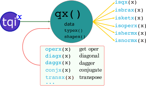
In bkgdtqix to represent such a quantum system $\mathcal{S}$, we construct a quantum object called bkgdqx, a matrix representation for quantum state and operators. An illustration of bkgdqx is given in Fig. 1. A quantum object contains the data about the given state or operator that it represents. Besides providing the data, it also allows us to check its type and dimension using bkgdtypex(x) and bkgdshapex(x), respectively. For example, in the following code, we generate a random state in the two-dimensional space and then check its type and dimension.

⬇

from tqix import *

a = random(2)

print(typex(a))

print(shapex(a))

where we get the output as

⬇

ket

(2, 1)

which means it is a ket (column) vector represented by a 2 x 1 matrix.

It is easy to convert a given instance x: (integer, real, complex, tuple, array,…) into a quantum object using bkgdqx(x) command, and its properties can be checked, including bar, ket, oper,… as listed in Table. 1. Furthermore, a library of commonly occurring operators is also built into bkgdtqix as listed in Table. 2 and allows for operating on the quantum objects. The structure of bkgdqx is quite similar to the bkgdQobj class in Qutip Johansson et al. (2012, 2013).

Figure 1: (Color online) Structure of a quantum object in tqix. A quantum object can be either a bra-ket vector or a matrice, which stands for quantum states or operators. In tqix, a quantum object is represented by a matrix. We can check its physical properties such as type, dimension, Hermitity, and more (see the full list in Table 1). Besides, one can also operate algebra transformations on the quantum object such as conjugate, transpose, and more (see the full list in Table 2).

Table 1: List of properties of a quantum object. We can easy to check the physical properties of a quantum object by using the list below.

Method	Description
isqx(x)	check whether x is a quantum object
isbrax(x)	check whether x is a bra vector
isketx(x)	check whether x is a ket vector
isoperx(x)	check whether x is an operator (mixed state, Hamiltonian,…)
ishermx(x)	check whether x is a Hermit
isnormx(x)	check whether x is normalized

Table 2: List for commonly occurring operators that are built into tqix. We can easy to perform these familiar operators on a quantum object.

Method	Description
operx(x)	convert a bra or ket vector into oper
diagx(x)	diagonalize matrix x
daggx(x)	get conjugate transpose of x: x†
conjx(x)	get conjugation of x: x∗
transx(x)	get transpose of x: xT
tracex(x)	get trace of x: (only for oper)
eigenx(x)	eigenvalue and eigenstate
groundx(x)	get ground state for a given Hamiltonian
expx(x)	exponentiated x
sqrtx(x)	square root of x
l2normx(x)	get norm 2 of x
normx(x)	get normalize of x

In subsections II.2 and II.3 following, we describe detailed quantum states and quantum operators in bkgdtqix.

II.2 Quantum states

It is straightforward to construct quantum states with some standard bases and conventional states that are built into bkgdtqix. The list of quantum states can be seen in A. Furthermore, to mimic a real quantum state that may contain systematic errors or technique error, bkgdtqix allows us to add a small error to the original quantum state:

$$|\psi\rangle\to|\psi^{\prime}\rangle=\dfrac{1}{\mathcal{N}}\sum_{n}(\psi_{n}+\delta_{n})|n\rangle,$$ (1)

where $\mathcal{N}$ a normalization constant, $\psi_{n}=\langle n|\psi\rangle$, and $\delta_{n}$ is a complex random noise following a normal distribution, e.g., $\delta_{n}=a+ib$, where $a,b$ are random numbers (noise). For example, we add small random noise into a GHZ state as follows:

⬇

from tqix import *

import numpy as np

psi = ghz(3)

psip = add_random_noise(psi, m = 0.0, st = 0.1)

Here, the random noise obeys a normal distribution with mean m and standard deviation st, defaulted be zeros. When the noise is presented, the quantum state will deviate from its original value. Such noisy systems are widespread in various practical situations  Watanabe et al. (2010); Harper et al. (2020).

For a mixed state, the error can be seen as a white-noise and is given by

$$\rho\to\rho^{\prime}=(1-p)\rho+p\bm{I}/d,$$ (2)

where $p$ is a small error ($0\leq p\leq 1$), and $d$ is the dimension of the system space. For example, one can easily add a small white noise to an original state (e.g., GHZ state) just with few lines as follows:

⬇

from tqix import *

rho = ghz(3)

rhop = add_white_noise(rho, p = 0.1)

where we have used p = 0.1 (its default value is zero). The function bkgdadd_white_noise executes Eq. (2) where its input state rho can be either pure or mixed state. An identity matrix $\bm{I}$ can be called from bkgdtqix by bkgdeyex(d).

We emphasize that other kinds of error can be defined and constructed by the users themselves, such as bit flip, phase flip, bit-phase flip, depolarizing, amplitude damping, and others (see detailed in Chap. 8 Ref. Nielsen and Chuang (2010)).

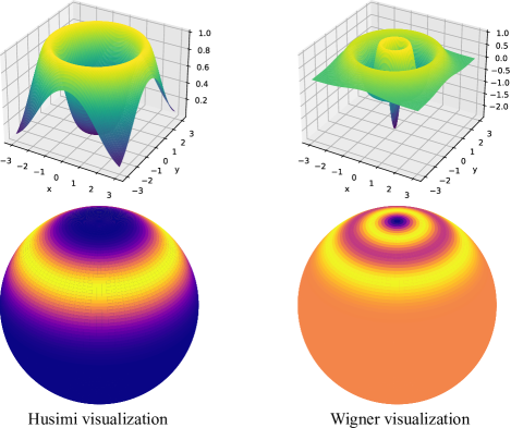
Visualization of quantum states. Phase-space representation is a powerful tool to visualize quantum states. Among various ways, the visualization using the Husimi function and Wigner function are two common methods that are widely used Schmied and Treutlein (2011); McConnell et al. (2015); Koczor et al. (2020); Ahmed et al. (2020).

In general, a 3-dimension (3D) Husimi function representation of a given state $\rho$ is $Q(\alpha)=\frac{1}{\pi}\langle\alpha|\rho|\alpha\rangle,$ where $|\alpha\rangle$ is the coherent state, and $\alpha=x+iy$ is a complex number. Similarly, the Wigner function is given by $W(\alpha)=\frac{2}{\pi}\sum_{k=0}^{\infty}(-1)^{k}\langle\alpha,k|\rho|\alpha,k\rangle,$ where $|\alpha,k\rangle=\bm{D}(\alpha)|k\rangle$ is the displaced number state, and $D(\alpha)$ is the displacement operator  Moya-Cessa and Knight (1993),

In particular cases of spin systems, it is more convenient to visualize the Husimi and Wigner functions in Bloch spheres. The Husimi function in a Bloch sphere is given by $Q(\theta,\phi)=\frac{1}{\pi}\langle\theta,\phi|\rho|\theta,\phi\rangle,$ where $|\theta,\phi\rangle$ is the spin coherent state, and $\theta,\phi$ are azimuthal and polar angles, respectively. The Wigner function in a Bloch sphere is expressed as  Dowling et al. (1994)

$$W(\theta,\phi)=\sum_{k=0}^{2j}\sum_{q=-k}^{k}\rho_{kq}\bm{Y}_{kq}(\theta,\phi)$$ (3)

where $Y_{kq}(\theta,\phi)$ is the spherical harmonic, and $\rho_{kq}=\sum_{m=-j}^{j}\sum_{m^{\prime}=-j}^{j}\rho_{mm^{\prime}}t_{kq}^{imm^{\prime}}$ is the quantum state represented in the spherical harmonics basis Schmied and Treutlein (2011). Here, $\rho_{mm^{\prime}}=\langle j,m|\rho|j,m^{\prime}\rangle$ is the quantum state represented in the Dicke basis $|j,m\rangle$, and $t_{kq}^{imm^{\prime}}=(-1)^{j-m-q}\langle j,m;j,-m^{\prime}|k,q\rangle$ is the Clebsch-Gordan coefficient  Dowling et al. (1994).

These visualizations are manipulated in bkgdtqix and are easy to use. For example, in Fig. 2, we visualize the Husimi and Wigner functions of a Dicke basis $|j,m\rangle$ in 3D and Bloch sphere. The visualization code is shown in C.

Figure 2: (Color online) The Husimi and Wigner visualizations of a Dicke basis $|j,m\rangle=|10,7\rangle$ in 3-dimension (upper row) and in the Bloch sphere (lower row).

II.3 Quantum operators

B represents some standard built-in quantum operators. In bkgdtqix, a defined operator can be either a Hamiltonian or an evolution operator, represented by a matrix. Also, to manipulate operators’ actions on quantum states or operate on multiple states, bkgdtqix builds various utility mathematical functions, including bkgddotx and bkgdtensorx for dot product and tensor product, respectively.

II.4 Construction of quantum systems in tqix

With those standard tools presented in subsections II.2 and II.3, we can straightforwardly construct a physical system with the given quantum state and Hamiltonian. For example, one can construct a two-level system state, e.g., $1/\sqrt{2}(|0\rangle+|1\rangle)$, and its unitary evolution, e.g., $\bm{U}=0.5\sigma_{z}-0.25\sigma_{x}$, by using the following code:

⬇

from tqix import *

from numpy import sqrt

state = 1/sqrt(2)*(obasis(2,0) + obasis(2,1))

U = 0.5*sigmaz() - 0.25*sigmax()

evolved_state = dotx(U,state) #U|psi>

Composite systems are also easy to create by using the bkgdtensorx function to generate tensor product states and combine Hilbert spaces. For example, let us consider a three-spin system with the initial state is $|\uparrow\uparrow\uparrow\rangle$, and the evolution is $\bm{U}=e^{-i\theta\sigma_{z}\sigma_{x}\sigma_{x}}$ where $\theta$ is a time-dependent phase. One can use the following bkgdtqix code to generate these objects:

⬇

from tqix import *

from numpy import pi

theta = pi/4 #for example

up = obasis(2,0) #spin up

state = tensorx(up,up,up)

H = tensorx(sigmaz(), sigmax(), sigmax())

U = expx(-1j*theta*H)

new_state = dotx(U,state)

Besides, to decompose a quantum object (state or operator), for example, $\rho_{\mathcal{AB}}$, on a composite space $\mathscr{H}_{\mathcal{A}}\otimes\mathscr{H}_{\mathcal{B}}$, onto a quantum object $\rho_{\mathcal{A}}$ on $\mathscr{H}_{\mathcal{A}}$, we can perform a partial trace using bkgdptracex syntax. It is a linear map $\rho_{\mathcal{A}}={\rm tr}_{\mathcal{B}}[\rho_{\mathcal{AB}}]$: $AB\to{\rm tr}(B)A$, for any matrices $A,B$ on $\mathscr{H}_{\mathcal{A}}$ and $\mathscr{H}_{\mathcal{B}}$, respectively. For example, one can trace out the second and third subsystems of the above Hamiltonian by using

⬇

H1 = ptracex(H,[2,3])

Here, we keep the first subsystem. Notable that in this version, bkgdptracex is only applicable for qubits systems.

III Quantum measurement

bkgdtqix mainly focuses on the calculation and simulation of quantum measurement for quantum systems. We first review the quantum measurement theory using the POVM formalism and then describe how this measurement is built into bkgdtqix. For simulating the measurement results, we also construct two available back-ends that can be executed in bkgdtqix.

III.1 General measurement

Quantum measurement is characterized by a set of measurement operators denoted by $\{M_{k}\}$ satisfying the completeness condition $\sum_{k}M^{\dagger}_{k}M_{k}=\bm{I}$, where $k$ is a measurement outcome. These measurement operators will operate on the quantum state of the measuring system. For a quantum system given in a general density state $\rho$, the probability to obtain the outcome $k$ is

$$p_{k}={\rm tr}[M^{\dagger}_{k}M_{k}\ \rho].$$ (4)

The quantum state after measurement will collapse to

$$\rho^{\prime}=\dfrac{M_{k}\rho M^{\dagger}_{k}}{{\rm tr}[M^{\dagger}_{k}M_{k}\ \rho]}.$$ (5)

Furthermore, a projective measurement $\bm{\Pi}$ is a special class of the general measurement that described by a Hermitian operator decomposing to

$$\bm{\Pi}=\sum_{k}k\Pi_{k},$$ (6)

where $\Pi_{k}\equiv|k\rangle\langle k|$ is a projection operator projected onto the eigenstate $|k\rangle$ of $\bm{\Pi}$ with eigenvalue $k$. For a projective measurement, the probability and the post-measurement state are calculated to be:

$$p_{k}={\rm tr}[\Pi_{k}\ \rho],\text{ and }\rho^{\prime}=\dfrac{\Pi_{k}\rho\Pi_{k}}{{\rm tr}[\Pi_{k}\ \rho]}.$$ (7)

See Ref. Nielsen and Chuang (2010) for more detailed quantum measurement.

III.2 Positive-Operator-Valued Measurement

In many practical cases, such as quantum tomography and quantum metrology, one may not need to care about the post-measurement state but rather focus on the measurement probability. In such cases, analyzing the measurement using a positive-operator-valued measure (POVM) is referred. POVM is a mathematical description of the measurement which is a consequence of the general measurement Nielsen and Chuang (2010). A POVM’s element, said $E_{k}$, is associated with the measurement $M_{k}$ by $M_{k}=W\sqrt{E_{k}}$, where $W$ an arbitrary unitary operator, or we can define

$$E_{k}=M_{k}^{\dagger}M_{k},$$ (8)

that is a positive operator satisfying the completeness relation $\sum_{k}E_{k}=\bm{I}$. The probability, in this case, is given by

$$p_{k}={\rm tr}[E_{k}\ \rho].$$ (9)

The POVM formalism is thus convenient for studying the statistics of the measurement without acknowledging the post-measurement state.

Pauli measurement set. In quantum measurements, one can usually combine several POVMs as a measurement set for characterizing properties of the system to be measured. One common choice is the Pauli measurement set. For one qubit, a measurement set $M$ consists of three POVMs as

$$\bigl{\{}M\bigr{\}}=\Bigl{\{}|H\rangle\langle H|,|V\rangle\langle V|,|D\rangle\langle D|,|A\rangle\langle A|,|L\rangle\langle L|,|R\rangle\langle R|\Bigr{\}},$$ (10)

where

$$|H\rangle=\begin{pmatrix}1\\ 0\end{pmatrix},\ |V\rangle=\begin{pmatrix}0\\ 1\end{pmatrix},$$

$$|D\rangle=\dfrac{1}{\sqrt{2}}\begin{pmatrix}1\\ 1\end{pmatrix},\ |A\rangle=\dfrac{1}{\sqrt{2}}\begin{pmatrix}1\\ -1\end{pmatrix},$$

and,

$$|L\rangle=\dfrac{1}{\sqrt{2}}\begin{pmatrix}1\\ i\end{pmatrix},\ |R\rangle=\dfrac{1}{\sqrt{2}}\begin{pmatrix}1\\ -i\end{pmatrix},$$

therein, $\{|H\rangle\langle H|,|V\rangle\langle V|\};\{|D\rangle\langle D|,|A\rangle\langle A|\}$; and $\{|L\rangle\langle L|,|R\rangle\langle R|\Bigr{\}}$ are the three POVMs. For an $n$-qubit system, the measurement set is formed by a tensor product of elements in $M$. There are $6^{n}$ elements in total, and thus it consumes much calculation cost and the experimental time.

Stoke measurement set. Another practical measurement set is based on a light beam’s polarization state, which was pioneering proposed by Stoke Stokes (1851). He showed that a single qubit system could be determined by a set of four projection measurements. These projection measurements can be chosen arbitrarily from six elements above James et al. (2001); Thew et al. (2002). In bkgdtqix, we choose $|H\rangle\langle H|,|V\rangle\langle V|,|D\rangle\langle D|,\text{ and }|R\rangle\langle R|$.

Likewise the Pauli measurement set, all the elements of $n$-qubit system can be found by using a tensor product of four projection measurements, which results in $4^{n}$ elements.

MUB-POVM set. Given two orthonormal bases $\{|e_{i}\rangle\}$ and $\{|f_{j}\rangle\}$ in a finite-dimensional Hilbert space $\mathscr{H}_{d}$, they are said to be mutually unbiased (MUB) if the inner product between any two elements in each basis is a constant Schwinger (1960):

$$\bigl{|}\langle e_{i}|f_{j}\rangle\bigr{|}^{2}=\dfrac{1}{d},\forall i,j\in[1,d].$$ (11)

For a $d$-dimensional Hilbert space, in general, there are $d+1$ POVMs and $d$ elements in each POVM. In total, it needs at least $d^{2}-1$ measurements, which is much smaller than the Pauli case.

There are several methods for finding MUB-POVMs across dimension $d$, including the Weyl group Bengtsson (2007), unitary operators Bandyopadhyay et al. (2002), and the Hadamard matrix method Bengtsson (2007). However, we omit writing them out here and encourage readers to refer DURT et al. (2010); Bengtsson (2007); Klappenecker and Rötteler (2004); Bandyopadhyay et al. (2002); Lawrence et al. (2002) if needed. In bkgdtqix, we have constructed several MUB-POVMs for $d=2,3,4,5,7$. In the future, we also plan to develop other cases.

SIC-POVM set. In a similar manner, a measurement set $\{|h_{i}\rangle\}$ is called symmetric informationally complete (SIC) when all the inner products between different elements are equal, and their projectors are complete Renes et al. (2004):

$$\bigl{|}\langle h_{i}|h_{j}\rangle\bigr{|}^{2}=\dfrac{1}{d+1},\forall i\neq j.$$ (12)

Notable that there is only one POVM in a SIC-POVM set with $d^{2}$ elements.

A most general way to construct a SIC-POVM is using the Weyl-Heisenberg displacement operators Weyl (1930); Scott and Grassl (2010); Bent et al. (2015):

$$D_{j,k}=\omega_{d}^{jk/2}\sum_{m=0}^{d-1}\omega_{d}^{jk}\bigl{|}k+m\text{ (mod d)}\big{\rangle}\big{\langle}m\bigr{|},$$ (13)

where $\omega_{d}=\exp(2\pi i/d)$. Then, a set of SIC-POVM elements can be calculated by applying the displacement operators on the fiducial vector $|\phi_{d}\rangle$. The fiducial vector construction has been carried out so far Appleby (2005); Grassl (2004); Renes et al. (2004); Gour and Kalev (2014); Scott and Grassl (2010); Grassl (2005) and is listed in Zauner . Such a list is also built into bkgdtqix.

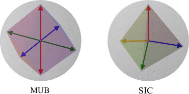
Besides the Pauli and Stoke measurement sets, the MUB-POVM and SIC-POVM measurement sets are also widely used in quantum theory Tavakoli et al. (2019); Bent et al. (2015); Rastegin (2013); Bengtsson (2010); Beneduci et al. (2013); Wootters (2006); Grassl (2004). In Fig. 3, we present a Bloch sphere representation of the two MUB and SIC measurement sets for one qubit ($d=2$). Note that for one qubit, the Pauli measurement set is the same as the MUB one. Six elements of MUB correspond to vertices of an octahedron, while four elements of SIC correspond to vertices of a tetrahedron.

Figure 3: (Color online) Bloch sphere representation of the MUB (a) and SIC (b) measurement sets for one qubit. Six measurements of MUB correspond to vertices of an octahedron, while four measurements of SIC correspond to vertices of a tetrahedron.

III.3 Quantum measurement in tqix

In bkgdtqix, one can calculate the probability for a given quantum system state and a set of observables (or POVMs) as the following example:

⬇

from tqix import *

state = ghz(1)

model = qmeas(state, [sigmax(),sigmay(),sigmaz()])

print(model.probability())

In this example, we calculate the expectation values $\langle\sigma_{x}\rangle,\langle\sigma_{y}\rangle,$ and $\langle\sigma_{z}\rangle$ of a given state $|\psi\rangle=1/\sqrt{2}(|0\rangle+|1\rangle)$. The outcomes are

⬇

[1.0, 0.0, 0.0]

Furthermore, bkgdtqix also contains the Pauli, Stoke, MUB-POVM, and SIC-POVM measurement sets. One can easy to call them out by a simple syntax, such as

⬇

model = qmeas(state, ’Pauli’)

For other measurement sets, one can replace bkgd’Pauli’ by bkgd’Stoke’, bkgd’MUB’, and bkgd’SIC’, respectively.

In Fig. 4, we compare the calculation time of different measurement sets for a random state in $d$ dimension. Particularly, we first generate a random quantum state. We then measure this state via different measurement sets, i.e., Pauli, Stoke, MUB-POVM, and SIC-POVM, and compare the execution time for each number of dimension $d$. See D for detailed code.

Figure 4: (Color online) The calculation time of different measurement sets. While Pauli measurement consumes much time, Stoke and MUB-POVM have an equivalence time, and SIC-POVM less consumes the time.

III.4 Back-end for simulation measurement results

A back-end is defined either as a simulator or a real device. For a given quantum object and a set of POVMs, a back-end is executed to simulatively retrieve the corresponding measurement results. In bkgdtqix, to mimic the real experiment data, we use several back-ends to simulate the results. A so-called Monte Carlo Rubinstein and Kroese (2017) (bkgdmc) back-end and Cumulative Distribution Function Gentle (2009) (bkgdcdf) back-end have been built into bkgdtqix. In the future, we will also construct such a back-end from real devices.

mc back-end. Particularly, a straightforward simulation back-end used in bkgdtqix is based on the Monte Carlo simulation method, which we named as bkgdmc back-end. Assume that a probability distribution of measurement is $f(x)$, generally, a function of $x$. Without loss of generality, we assume that $0\leq f(x)\leq 1,\forall x$, (a physical probability does not exceed the range of [0, 1].) For each given $f(k),k\in\{x\}$, the following procedure is processed:
(i) generate a random number $r$ following a uniform distribution within [0, 1],
(ii) accept $r$ if $r\leq f(k)$,
(iii) repeat (i, ii) $N_{c}$ times to get the frequency between the number of accepted $r$ and $N_{c}$, which will distribute according to $f(k)$. This method has been used in quantum state tomography, for example, see Refs. Schwemmer et al. (2015); Faist and Renner (2016).

cdf back-end. Another back-end is named as bkgdcdf based on the cumulative distribution function (cdf). For a given probability distribution of a measurement $f(x)$, the cdf function is defined to be

$$F(y)=\int_{-\infty}^{y}f(x)dx.$$ (14)

Given a uniform random variable $r\in[0,1]$ then $y=F^{-1}(r)$ is distributed following $f(x)$. Like the bkgdmc back-end, this method has also been widely used in quantum state tomography  Maccone and Rusconi (2014); Ho (2020, 2019); Tuan et al. (2020).

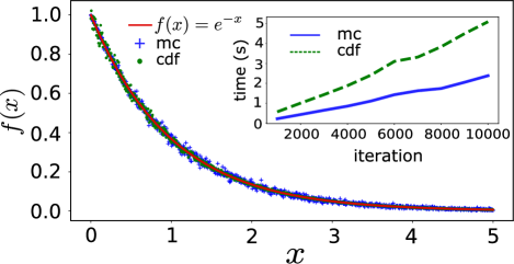
As an example, let us choose $f(x)=e^{-x},x>0$, and therefore the cumulative distribution is $F(y)=1-e^{-y}$. Then, for a random number $r$, the corresponding $y$ yields:

$$y=-ln(1-r),$$ (15)

which distributes according to $f(x)$.

In Fig. 5, we plot $f(x)$ and its simulation results via the bkgdmc and bkgdcdf back-ends. Refer to E for detailed coding. While the bkgdcdf back-end is more accurate than the bkgdmc, the cost that one has to pay is that it consumes more time than the bkgdmc back-end (see the inset figure.) For some simulation tasks that require sufficient accuracy, we encourage the users to employ the bkgdcdf back-end.

Figure 5: (Color online) Plot of $f(x)$ versus mc and cdf back-ends. Inset: the simulation time for mc and cdf back-ends. While the cdf back-end is more accurate than the mc back-end, it also consumes more time than the mc one.

IV Quantum state tomography

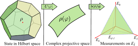
In general, the quantum state tomography (QST) is a process that reconstructing the information of unknown quantum states from the measurement data Paris and Řeháček (Eds). The tomography procedure is illustrated in Fig. 6. A quantum state, for example $|\psi\rangle$, is presented in its Hilbert space as given on the left side of the figure. Here, for a $d$-dimensional Hilbert space, the state is expressed by

$$|\psi\rangle=\sum_{n=0}^{d-1}\psi_{n}|n\rangle,$$ (16)

where $\psi_{n}$ are unknown parameters need to be estimated, and $\{|n\rangle\}$ is a computational basis on the Hilbert space. The state is measured in a measurement set, e.g., $\{E_{0},E_{1},\dots\}$ as illustrated in the middle of Fig. 6. The measurement set can be chosen from one of those described in Sec. III. Finally, the measurement results will be analyzed via an estimator such as maximum likelihood (ML) Hradil (1997), least squares (LS) James et al. (2001), neural network Torlai et al. (2018); Xin et al. (2019); Weiss and Romero-Isart (2019); Liu et al. (2020); Xu and Xu (2018); Quek et al. (2018), and others, to reproduce the state. The reconstructed state is denoted by $|\tilde{\psi}\rangle$, where

$$|\tilde{\psi}\rangle=\sum_{n=0}^{d-1}\tilde{\psi}_{n}|n\rangle.$$ (17)

Figure 6: (Color online) Quantum state tomography process: (i) A quantum state $|\psi\rangle$ is unknown and expressed in its Hilbert space of $d$ dimension. (ii) The state is measured in a measurmement set given by $E_{0},E_{1},\dots$. (iii) The measurement results provide the information of the measuring state via an estimator, such as ML, LS, and so forth. The reconstructed state is $|\tilde{\psi}\rangle=\sum\tilde{\psi}_{n}|n\rangle$.

To evaluate the accuracy of the tomography process, one can compare the true state $|\psi\rangle$ and the reconstructed state $|\tilde{\psi}\rangle$ via the various figure of merits such as the trace distance and the fidelity. The trace distance between $|\psi\rangle$ and $|\tilde{\psi}\rangle$ is given by

$$D(\psi,\tilde{\psi})=\sqrt{1-\bigl{|}\langle\tilde{\psi}|\psi\rangle\bigr{|}^{2}}\;.$$ (18)

For general mixed states $\rho$ and $\tilde{\rho}$, the trace distance is given by Nielsen and Chuang (2010)

$$D(\rho,\tilde{\rho})=\dfrac{1}{2}{\text{tr}}\ \bigl{|}\tilde{\rho}-\rho\bigr{|}\;.$$ (19)

Moreover, the fidelity is given by Nielsen and Chuang (2010)

$$F(\rho,\tilde{\rho})={\rm tr}\sqrt{\sqrt{\rho}\tilde{\rho}\sqrt{\rho}}\;.$$ (20)

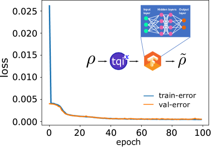
Now, we give an example of using bkgdtqix in QST. Assume that a given system is described by a quantum state $\rho$ that we want to reconstruct. Using bkgdtqix as given in Sec. III.3, we can get the measurement probabilities. From those measurement data, we reproduce the quantum state. Here, in this example, we use a neural network scheme to reconstruct the quantum state, which is also widely used recently in the QST Torlai et al. (2018); Xin et al. (2019); Weiss and Romero-Isart (2019); Liu et al. (2020); Xu and Xu (2018); Quek et al. (2018). We build a neural network consists of four layers: an input layer, two hidden layers, and an output layer using bkgdTensorflow. The input layer was fed by the set of outcome probabilities obtained from bkgdtqix, while the output layer is the quantum state of being reconstructed. These layers were connected via a $tanh$ cost function. Our scheme is illustrated in the inset Fig. 7. In Fig. 7, we also show an example of the loss model while training the experiment data from bkgdtqix with the Pauli measurement set.

Figure 7: (Color online) Test of loss function for training data and validation data in Tensorflow. There is no overfitting in this example (the training error and the validation error are close.) Inset: tomography scheme: given an unknown state $\rho$, through tqix, we obtain the set of measurement results that can be fed into a neural network build-in Tensorflow. From the Tensorflow’s output, we can reconstruct the given quantum state, named as $\tilde{\rho}$.

Besides, bkgdtqix also has been used to reconstruct the quantum state using the direct state measurement (DSM) method. For references, we encourage readers to see Refs. Ho (2020, 2019); Tuan et al. (2020).

V Quantum metrology

Quantum metrology is a process that unknown (single or multiples) parameters are estimated from a set of measurements  Giovannetti et al. (2011); Pezzè et al. (2018). The process is illustrated in Fig. 8 for a single parameter estimation. First, a system is prepared in a general mixed density state $\rho$. The state will acquire a phase $\varphi$ after being exposed under an external field represented by a unitary transformation $\bm{U}(\varphi)=e^{-i\varphi\bm{H}}$ and transforms to $\rho(\varphi)=\bm{U}(\varphi)\rho\bm{U}^{\dagger}(\varphi)$. Here, $\bm{H}$ is a generic Hermitian operator. The system after that will be measured via a POVM $\{E_{k}\}$, and the results allow for estimating the unknown parameter $\varphi$.

The measurement precision (variance) $\Delta\varphi$ after $N$ independent measurements is defined by $\Delta\varphi=\sqrt{\langle(\varphi-\tilde{\varphi})^{2}}\rangle$, where $\tilde{\varphi}$ is the estimated value. The minimum of $\Delta\varphi$ is bounded by the Cramér-Rao bounds

$$\Delta\varphi\geq\dfrac{1}{\sqrt{NF}}\geq\dfrac{1}{\sqrt{NQ}},$$ (21)

where $F$ and $Q$ are the classical and quantum Fisher information, respectively, which are defined by  Braunstein and Caves (1994)

$$F =\sum_{k}\dfrac{1}{p_{k}(\varphi)}\Bigl{[}\dfrac{\partial p_{k}(\varphi)}{\partial\varphi}\Bigr{]}^{2},$$ (22)

$$Q =2\sum_{m,n}\dfrac{(q_{m}-q_{n})^{2}}{q_{m}+q_{n}}\bigl{|}\langle m|\bm{H}|n\rangle\bigr{|}^{2}.$$ (23)

Here, the probability of a measurement $E_{k}$ is given by $p_{k}(\varphi)={\rm tr}[E_{k}\ \rho(\varphi)],$ as in Eq. (7), and the density state $\rho(\varphi)$ is given in its spectral decomposed form, i.e., $\rho(\varphi)=\sum_{m}q_{m}|m\rangle\langle m|$, where $q_{m}$ and $|m\rangle$ are eigenvalues and eigenvectors, respectively.

The first inequality in Eq. 21 is classical Cramér-Rao bound (CCRB) while the second one is quantum Cramér-Rao bound (QCRB). In the single parameter estimation, the CCRB is saturated by the maximum likelihood estimator asymptotically in the number of repeated measurements [$N$ in Eq. (21)], and the QCRB is saturated by using an optimal measurement observable, which is given by the projection over the eigenstates of the symmetric logarithmic derivatives (SLD) (see Refs. Braunstein (1992); Braunstein and Caves (1994); Giovannetti et al. (2011); Pezzè et al. (2018)). Furthermore, $\Delta\varphi$ reaches the standard quantum limit (SQL) precision scaling if it is proportional to $1/\sqrt{N}$, while it reaches the Heisenberg limit (HL) when $\Delta\varphi\propto 1/N$.

Figure 8: (Color online) Quantum metrology process: (i) A quantum system given in its density state $\rho$. (ii) The system is exposed under an external field given by $\bm{U}(\varphi)$ where $\varphi$ is an unknown field parameter and becomes $\rho(\varphi)$. (iii) The state $\rho(\varphi)$ is measured in a measurement set given by $E_{0},E_{1},\dots$ and provides the information on the estimated parameter $\varphi$.

Hereafter, we provide an example for studying quantum metrology using bkgdtqix. In our example, we consider a cat state quantum system, which is the superposition of spin-$j$ coherent states Huang et al. (2015, 2018a)

$$|\psi\rangle=\mathcal{N}\Bigl{(}|\theta,\phi\rangle+|\pi-\theta,\phi\rangle\Bigr{)},$$ (24)

where $\mathcal{N}$ is the normalization constant and $|\theta,\phi\rangle$ is a spin-$j$ coherent state Ho and Kondo (2019)

$$|\theta,\phi\rangle=\sum_{m=-j}^{j}c_{m}\cos^{j+m}\Bigl{(}\frac{\theta}{2}\Bigr{)}\sin^{j-m}\Bigl{(}\frac{\theta}{2}\Bigr{)}e^{-i(j-m)\phi}|j,m\rangle,$$ (25)

where $c_{m}=\sqrt{\dfrac{(2j)!}{(j+m)!(j-m)!}}$. Without loss of generality, we can choose $\phi=0$. Here, $|j,m\rangle$ is the standard angular momentum basis with the angular momentum quantum number $j=0,1/2,1,\dots$, and $m=-j,-j+1,\dots,j$ Lee Loh and Kim (2015).

Under the transformation $\bm{U}(\varphi)=e^{-i\varphi\bm{S}_{z}}$, the system evolves to $|\psi(\varphi\rangle=\bm{U}(\varphi)|\psi\rangle$. We then, evaluate the measurement precision by Huang et al. (2018b)

$$\Delta\varphi=\dfrac{\sqrt{\langle\bm{S}_{y}^{2}\rangle-\langle\bm{S}_{y}\rangle^{2}}}{|\partial\langle\bm{S}_{y}\rangle/\partial\varphi|},$$ (26)

where $\bm{S}_{k}$ ($k=x,y,z,+,-$) is a spin operator.

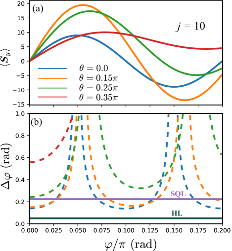
In Fig. 9, we show the expectation values $\langle\bm{S}_{y}\rangle$ (a) and $\Delta\varphi$ (b) as functions of $\varphi$. Here, we examine several values of $\theta$ as shown in the figure. We can see that the variance $\Delta\varphi$ can reach the minimum at an optimized value for $\varphi$. We emphasize that $\varphi$ is a function of the exposing time (the time that we expose the system under the external field), and thus there exists an optimal time that the variance is minimum. Interestingly, we can see that for $\theta=0.0$ and $0.15\pi$ the minimum variance can beat the SQL. This example is in agreement with Ref. Huang et al. (2018b). The code for generating Fig. 9 is shown in  F.

Figure 9: (Color online) (a) Plot of expectation value $\langle\bm{S}_{y}\rangle$ as a function of $\varphi$. We show the results for several values of $\theta$ as in the figure. Here we fix $j=10$. (b) Plot of the variance $\Delta\varphi$ as a function of $\varphi$. Several results are plotted with the same $\theta$ in (a). The SQL and HL are also shown in the figure.

VI Limitation of the program

Within the initial version of the program, we cannot cover all the existing quantum objects (quantum states and operators) here. We limit ourselves to some basic and useful quantum objects as mentioned throughout the paper. Further developed versions will improve and complement these lacking parts.

In quantum measurement, the program limits on some practical POVM sets, such as Pauli, Stoke, MUB-POVM, and SIC-POVM measurement sets, which are widely used in quantum theory and can be carried out in various experiments. Besides, the MUB-POVM has been constructed for $d$ = 2, 3, 4, 5, 7, where higher dimensions (to our knowledge) do not exist yet.

In the context of quantum tomography, the example program is limited to getting meaningful quantum states such as GHZ, W, and Dicke states. However, we emphasize that the program can be used for estimating any given quantum states, including non-classical states, such as coherent state, squeezes state, spin-coherent state, and others. Here, we highlight several example calculations to provide the readers with an overview of the program. Various tutorials can be found on the websites.

VII Conclusion

We have presented a computer program bkgdtqix by using the Python programming language and applied to the quantum measurement, quantum tomography, and quantum metrology. In this work, we have constructed a basic structure and some quantum features of a quantum object which can be used for both quantum states and quantum observables. There are several back-ends have been constructed for simulation in quantum measurement. Thus, this program is applicable for a spacious range in quantum measurement, quantum tomography, and quantum metrology. We strongly encourage those who have used this program to feedback (if any) error or incorrect to us for further developing the program.

Appendix A List of quantum states build-in tqix

In this appendix, we summary some useful quantum states used in the program. In the future, we also build other quantum states to the code.

Table 3: List of quantum states are built-in tqix

Name	Description
obasis(d,k)	orthogonal basis with $d$-dimension, excited at $k$, such as obasis(3,0) = $\begin{pmatrix}1\\ 0\\ 0\end{pmatrix}$, obasis(3,1) =$\begin{pmatrix}0\\ 1\\ 0\end{pmatrix}$,…
dbasis(d,k)	dual basis for the basis obasis
zbasis(j, m)	Zeeman basis or Dicke basis $|j,m\rangle$ with spin number $j$ and quantum number $m\in[-j,j]$.
dzbasis(j, m)	dual basis for the Zeeman basis zbasis.
coherent(d, alpha)	generating coherent state that cut off at $d$ dimension: $|\alpha\rangle=e^{-\frac{|\alpha|^{2}}{2}}\sum_{n=0}^{d}\frac{\alpha^{n}}{\sqrt{n!}}|n\rangle$, where $\alpha$ is a complex number provided by alpha, and $\{|n\rangle\}$ is the Fock (number) basis.
squeezed(d, alpha, beta)	generating squeezed coherent state that cut off at $d$ dimension: $|\alpha,\beta\rangle=e^{\alpha\bm{a}^{\dagger}-\alpha^{*}\bm{a}}e^{\frac{1}{2}(\beta^{*}\bm{a}^{2}-{\beta\bm{a}^{\dagger}}^{2})}|0\rangle$, where $\bm{a},\bm{a}^{\dagger}$ are annihilation and creation operators, respectively; $\alpha,\beta$ are complex numbers.
position(d, x)	generating position state which is an eigenstate of position operator $\bm{x}$, i.e., $\bm{x}|x\rangle=x|x\rangle$.
spin_coherent(j, theta, phi)	generating spin coherent state as given in Eq. (25).
random(d)	random state with $d$-dimension following Haar measure.
ghz(n)	generating GHZ state with $n$ qubits, i.e., $\frac{1}{\sqrt{2}}(|00\cdots 0\rangle+|11\cdots 1\rangle)$.
w(n)	generating W state with $n$ qubits, i.e., $\frac{1}{\sqrt{n}}(10\cdots 0\rangle+|01\cdots 0\rangle+\cdots+|0\cdots 01\rangle)$.
dicke(n,k)	generating Dicke state with $n$ qubits, $k$ excited qubits, i.e., $D(n,k)={n\choose k}^{-\frac{1}{2}}\sum_{x\in\{0,1\}^{n}}|x\rangle$. For example, $D(3,2)=\frac{1}{\sqrt{3}}(|011\rangle+|101\rangle+|110\rangle)$.

Appendix B List of quantum operators build-in tqix

Table 4: List of quantum operators build-in tqix

Name	Description
eyex(d)	identify matrix in $d$-dimension
soper(s,*)	spin-s operators with option *args can be $x,y,z,+,-$. soper(s) will return an array of spins $x,y,z$
sigmax()	Pauli matrix $\sigma_{x}$
sigmay()	Pauli matrix $\sigma_{y}$
sigmaz()	Pauli matrix $\sigma_{z}$
sigmap()	$\sigma_{+}$
sigmam()	$\sigma_{-}$
lowering(d)	lowering (or annihilation) operator in d dimension
raising(d)	raising (or creation) operator in d dimension
displacement(d, alpha)	displacement operator that cut off at $d$ dimension: i.e., $\bm{D}(\alpha)=e^{\alpha\bm{a}^{\dagger}-\alpha^{*}\bm{a}}$.
squeezing(d, beta)	squeezing operator that cut off at $d$ dimension: i.e., $\bm{S}(\beta)=e^{\frac{1}{2}(\beta^{*}\bm{a}^{2}-{\beta\bm{a}^{\dagger}}^{2})}$.

Appendix C Code for Husimi and Wigner visualizations (Figure 2)

⬇

from tqix import *

import numpy as np

psi = zbasis(10,7)

# 3d visualization

x = [-3, 3]

y = [-3, 3]

husimi_3d(psi, x ,y ,cmap = cmindex(1),fname =’husimi3d.eps’)

wigner_3d(psi, x ,y ,cmap = cmindex(1),fname =’wigner3d.eps’)

# Bloch sphere visualization

THETA = [0, np.pi]

PHI = [0, 2* np.pi]

husimi_spin_3d(psi, THETA ,PHI ,cmap = cmindex(1),fname = ’husimi_sphere.eps’)

wigner_spin_3d(psi, THETA ,PHI ,cmap = cmindex(1),fname = ’wigner_sphere.eps’)

For cmap, it is ranged from cmindex(1) to cmindex(82) or listed in cma .

Appendix D Code for calculation time of POVM sets (Figure 4)

⬇

import time

import numpy as np

from tqix import *

import matplotlib.pyplot as plt

N = 100 # number of repeated measurement

# For Pauli and Stoke

dim_p,time_p = [],[]

time_s = [],

for n in range (1,4):

#n: number of quibts

dtime_p = 0.0

dtime_s = 0.0

for i in range(N):

state = random(2**n)

###

model = qmeas(state,’Pauli’)

dtime = model.mtime() #measure time

dtime_p += dtime

model = qmeas(state,’Stoke’)

dtime = model.mtime()

dtime_s += dtime

dtime_p /= float(N)

dtime_s /= float(N)

dim_p.append(2**n)

time_p.append(dtime_p)

time_s.append(dtime_s)

# For MUB

dim_mub,time_mub = [],[]

for d in (2,3,4,5,7):

dtime_mub = 0.0

for i in range(N):

state = random(d)

###

model = qmeas(state,’MUB’)

dtime = model.mtime()

dtime_mub += dtime

dtime_mub /= float(N)

dim_mub.append(d)

time_mub.append(dtime_mub)

# For SIC

dim_sic, time_sic = [],[]

for d in range(2,9):

dtime_sic = 0.0

for i in range(N):

state = random(d)

###

model = qmeas(state,’SIC’)

dtime = model.mtime()

dtime_sic += dtime

dtime_sic /= float(N)

dim_sic.append(d)

time_sic.append(dtime_sic)

# Plot figure

fig, ax1 = plt.subplots(figsize=(12,6))

ax1.plot(dim_p, time_p, marker = ’o’)

ax1.plot(dim_p, time_s, marker = ’^’)

ax1.plot(dim_mub, time_mub, marker = ’s’)

ax1.plot(dim_sic, time_sic, marker = ’v’)

ax1.legend((’pauli’,’stoke’,’mub’,’sic’))

ax1.set_xlabel(’d’)

ax1.set_ylabel(’time (s)’)

plt.savefig(’time_povm.eps’)

plt.show()

Appendix E Code for back-ends (Figure 5)

⬇

from tqix import *

import numpy as np

import matplotlib.pyplot as plt

import time

def func(n):

fx = []

x = np.linspace(0,5,n)

for i in range(n):

fx.append(np.exp(-x[i]))

return fx

samp = 1000 #number of sample

ite = 1000 #number iteration

fx = func(samp)

mc_sim = []

cdf_sim = []

for i in fx:

mc_sim.append(mc(i,ite))

for i in fx:

temp = []

for j in range(ite):

temp.append(randunit()/i)

cdf_sim.append(cdf(temp))

x = np.linspace(0,5,samp)

fig, ax = plt.subplots(figsize=(12,6))

ax.plot(x,mc_sim,’b+’)

ax.plot(x,cdf_sim,’g.’)

ax.plot(x, fx, ’r’)

ax.legend(("mc","cdf","fx"))

ax.set_xlabel(’x’)

ax.set_ylabel(’exponential’);

plt.savefig(’fig5.eps’)

plt.show()

# time check

mc_times = []

cdf_times = []

ites = []

for ite in range(1000,11000,1000):

mc_start = time.time()

for i in fx:

mc_sim.append(mc(i,ite))

mc_stop = time.time()

delta = mc_stop - mc_start

mc_times.append(delta)

cdf_start = time.time()

for i in fx:

temp = []

for j in range(ite):

temp.append(randunit()/i)

cdf_sim.append(cdf(temp))

cdf_stop = time.time()

delta = cdf_stop - cdf_start

cdf_times.append(delta)

ites.append(ite)

fig, ax1 = plt.subplots(figsize=(12,6))

ax1.plot(ites, mc_times, ’r’)

ax1.plot(ites, cdf_times,’b--’)

ax1.legend(("mc","cdf"))

ax1.set_xlabel(’iteration’)

ax1.set_ylabel(’time (s)’)

plt.savefig(’inset.eps’)

plt.show()

Appendix F Code for quantum metrology (Figure 9)

⬇

from tqix import *

from numpy import pi

import matplotlib.pyplot as plt

n = 20

j = n/2

# spin cat state

def cat(j,theta,phi):

sc = spin_coherent(j,theta,phi)

scm = spin_coherent(j,pi-theta,phi)

s = normx(sc + scm)

return s

# spin observable

# j3[0] = S_x, j3[1] = S_y, j3[2] = S_z

j3 = soper(j)

def u(x):

return np.exp(-1j*x*j3[2])

t = np.linspace(0, 0.2, 100)

theta = [0.0, 0.15*pi, 0.25*pi, 0.35*pi]

phi = 0.0

# open figures

f1 = plt.figure()

f2 = plt.figure()

ax1 = f1.add_subplot(111,aspect = 0.003)

ax2 = f2.add_subplot(111,aspect = 0.115)

for i in theta:

r, r2, dt = [], [], []

for k in t:

#expectation value j3[1] and j3[1]**2

model = qmeas(dotx(u(k*pi),cat(j,i,phi)), [j3[1],j3[1]**2])

ex1 = model.probability()[0]

ex2 = model.probability()[1]

r.append(ex1)

r2.append(ex2)

dt.append(np.sqrt(np.abs(ex2-ex1**2)))

#differential dr and delta_varphi

dr = ndiff(t,r)

dp = dt/np.abs(dr)

#plot

ax1.plot(t,r,’-’)

ax2.plot(t,dp,’--’)

#standard quantum limit and Heisenberg limit

sql = 1./np.sqrt(float(n))*np.ones(t.shape)

hl = 1./float(n)*np.ones(t.shape)

ax2.plot(t,sql)

ax2.plot(t,hl)

plt.ylim(0,1)

plt.show()

References

- Busch et al. (2018) P. Busch, P. Lahti, P. Juha-Pekka, and K. Ylinen, Quantum Measurement (Springer International Publishing, 2018).
- Nielsen and Chuang (2010) M. A. Nielsen and I. L. Chuang, Quantum computation and quantum information (Cambridge University Press, 2010).
- Wheeler and Zurek (2014) J. A. Wheeler and W. H. Zurek, Quantum theory and measurement (Princeton University Press, 2014).
- Paris and Řeháček (Eds) M. Paris and J. Řeháček (Eds), Quantum State Estimation, Lecture Notes in Physics, Vol. 649 (Springer-Verlag, Berlin Heidelberg, 2004).
- Giovannetti et al. (2011) V. Giovannetti, S. Lloyd, and L. Maccone, Nature Photonics 5, 222 (2011).
- Pezzè et al. (2018) L. Pezzè, A. Smerzi, M. K. Oberthaler, R. Schmied, and P. Treutlein, Rev. Mod. Phys. 90, 035005 (2018).
- Magaña-Loaiza and Boyd (2019) O. S. Magaña-Loaiza and R. W. Boyd, Reports on Progress in Physics 82, 124401 (2019).
- Degen et al. (2017) C. L. Degen, F. Reinhard, and P. Cappellaro, Rev. Mod. Phys. 89, 035002 (2017).
- Kok et al. (2007) P. Kok, W. J. Munro, K. Nemoto, T. C. Ralph, J. P. Dowling, and G. J. Milburn, Rev. Mod. Phys. 79, 135 (2007).
- Childs and van Dam (2010) A. M. Childs and W. van Dam, Rev. Mod. Phys. 82, 1 (2010).
- Pirandola et al. (2019) S. Pirandola, U. L. Andersen, L. Banchi, M. Berta, D. Bunandar, R. Colbeck, D. Englund, T. Gehring, C. Lupo, C. Ottaviani, J. Pereira, M. Razavi, J. S. Shaari, M. Tomamichel, V. C. Usenko, G. Vallone, P. Villoresi, and P. Wallden, “Advances in quantum cryptography,” (2019), arXiv:1906.01645 [quant-ph] .
- James et al. (2001) D. F. V. James, P. G. Kwiat, W. J. Munro, and A. G. White, Phys. Rev. A 64, 052312 (2001).
- Helsen et al. (2019) J. Helsen, X. Xue, L. M. K. Vandersypen, and S. Wehner, npj Quantum Information 5, 71 (2019).
- Frank et al. (2017) F. Frank, T. Unden, J. Zoller, R. S. Said, T. Calarco, S. Montangero, B. Naydenov, and F. Jelezko, npj Quantum Information 3, 48 (2017).
- Gheorghiu et al. (2019) A. Gheorghiu, T. Kapourniotis, and E. Kashefi, Theory of Computing Systems 63, 715 (2019).
- Note (1) A measurement set contains one or several positive-operator-valued measures (POVMs).
- Johansson et al. (2012) J. Johansson, P. Nation, and F. Nori, Computer Physics Communications 183, 1760 (2012).
- Johansson et al. (2013) J. Johansson, P. Nation, and F. Nori, Computer Physics Communications 184, 1234 (2013).
- Radtke and Fritzsche (2008) T. Radtke and S. Fritzsche, Computer Physics Communications 179, 647 (2008).
- Radtke and Fritzsche (2010) T. Radtke and S. Fritzsche, Computer Physics Communications 181, 440 (2010).
- Fritzsche (2014) S. Fritzsche, Computer Physics Communications 185, 1697 (2014).
- Watanabe et al. (2010) Y. Watanabe, T. Sagawa, and M. Ueda, Phys. Rev. Lett. 104, 020401 (2010).
- Harper et al. (2020) R. Harper, S. T. Flammia, and J. J. Wallman, Nature Physics (2020), 10.1038/s41567-020-0992-8.
- Schmied and Treutlein (2011) R. Schmied and P. Treutlein, New Journal of Physics 13, 065019 (2011).
- McConnell et al. (2015) R. McConnell, H. Zhang, J. Hu, S. Ćuk, and V. Vuletić, Nature 519, 439 (2015).
- Koczor et al. (2020) B. Koczor, R. Zeier, and S. J. Glaser, Phys. Rev. A 101, 022318 (2020).
- Ahmed et al. (2020) S. Ahmed, C. S. Muñoz, F. Nori, and A. F. Kockum, “Classification and reconstruction of optical quantum states with deep neural networks,” (2020), arXiv:2012.02185 [quant-ph] .
- Moya-Cessa and Knight (1993) H. Moya-Cessa and P. L. Knight, Phys. Rev. A 48, 2479 (1993).
- Dowling et al. (1994) J. P. Dowling, G. S. Agarwal, and W. P. Schleich, Phys. Rev. A 49, 4101 (1994).
- Stokes (1851) G. G. Stokes, Transactions of the Cambridge Philosophical Society 9, 399 (1851).
- Thew et al. (2002) R. T. Thew, K. Nemoto, A. G. White, and W. J. Munro, Phys. Rev. A 66, 012303 (2002).
- Schwinger (1960) J. Schwinger, Proceedings of the National Academy of Sciences 46, 570 (1960), https://www.pnas.org/content/46/4/570.full.pdf .
- Bengtsson (2007) I. Bengtsson, AIP Conference Proceedings 889, 40 (2007), https://aip.scitation.org/doi/pdf/10.1063/1.2713445 .
- Bandyopadhyay et al. (2002) Bandyopadhyay, Boykin, Roychowdhury, and Vatan, Algorithmica 34, 512 (2002).
- DURT et al. (2010) T. DURT, B.-G. ENGLERT, I. BENGTSSON, and K. ŻYCZKOWSKI, International Journal of Quantum Information 08, 535 (2010), https://doi.org/10.1142/S0219749910006502 .
- Klappenecker and Rötteler (2004) A. Klappenecker and M. Rötteler, in Finite Fields and Applications, edited by G. L. Mullen, A. Poli, and H. Stichtenoth (Springer Berlin Heidelberg, Berlin, Heidelberg, 2004) pp. 137–144.
- Lawrence et al. (2002) J. Lawrence, i. c. v. Brukner, and A. Zeilinger, Phys. Rev. A 65, 032320 (2002).
- Renes et al. (2004) J. M. Renes, R. Blume-Kohout, A. J. Scott, and C. M. Caves, Journal of Mathematical Physics 45, 2171 (2004), https://doi.org/10.1063/1.1737053 .
- Weyl (1930) H. M. Weyl, The theory of groups and quantum mechanics: Transl. from the second (rev.) German ed. by H.P. Robertson. With 3 diagrams (Dover Publ., 1930).
- Scott and Grassl (2010) A. J. Scott and M. Grassl, Journal of Mathematical Physics 51, 042203 (2010), https://doi.org/10.1063/1.3374022 .
- Bent et al. (2015) N. Bent, H. Qassim, A. A. Tahir, D. Sych, G. Leuchs, L. L. Sánchez-Soto, E. Karimi, and R. W. Boyd, Phys. Rev. X 5, 041006 (2015).
- Appleby (2005) D. M. Appleby, Journal of Mathematical Physics 46, 052107 (2005), https://doi.org/10.1063/1.1896384 .
- Grassl (2004) M. Grassl, “On sic-povms and mubs in dimension 6,” (2004), arXiv:quant-ph/0406175 [quant-ph] .
- Gour and Kalev (2014) G. Gour and A. Kalev, Journal of Physics A: Mathematical and Theoretical 47, 335302 (2014).
- Grassl (2005) M. Grassl, Electronic Notes in Discrete Mathematics 20, 151 (2005), proceedings of the Workshop on Discrete Tomography and its Applications.
- (46) G. Zauner, “External links,” .
- Tavakoli et al. (2019) A. Tavakoli, M. Farkas, D. Rosset, J.-D. Bancal, and J. Kaniewski, “Mutually unbiased bases and symmetric informationally complete measurements in bell experiments: Bell inequalities, device-independent certification and applications,” (2019), arXiv:1912.03225 [quant-ph] .
- Rastegin (2013) A. E. Rastegin, The European Physical Journal D 67, 269 (2013).
- Bengtsson (2010) I. Bengtsson, Journal of Physics: Conference Series 254, 012007 (2010).
- Beneduci et al. (2013) R. Beneduci, T. J. Bullock, P. Busch, C. Carmeli, T. Heinosaari, and A. Toigo, Phys. Rev. A 88, 032312 (2013).
- Wootters (2006) W. K. Wootters, Foundations of Physics 36, 112 (2006).
- Rubinstein and Kroese (2017) R. Y. Rubinstein and D. P. Kroese, Simulation and the Monte Carlo method (Wiley., 2017).
- Gentle (2009) K. E. Gentle, Computational Statistics (Springer, 2009).
- Schwemmer et al. (2015) C. Schwemmer, L. Knips, D. Richart, H. Weinfurter, T. Moroder, M. Kleinmann, and O. Gühne, Phys. Rev. Lett. 114, 080403 (2015).
- Faist and Renner (2016) P. Faist and R. Renner, Phys. Rev. Lett. 117, 010404 (2016).
- Maccone and Rusconi (2014) L. Maccone and C. C. Rusconi, Phys. Rev. A 89, 022122 (2014).
- Ho (2020) L. B. Ho, Journal of Physics B: Atomic, Molecular and Optical Physics 53, 115501 (2020).
- Ho (2019) L. B. Ho, Physics Letters A 383, 289 (2019).
- Tuan et al. (2020) K. Q. Tuan, H. Q. Nguyen, and L. B. Ho, “Direct state measurements under state-preparation-and-measurement errors,” (2020), arXiv:2007.05294 [quant-ph] .
- Hradil (1997) Z. Hradil, Phys. Rev. A 55, R1561 (1997).
- Torlai et al. (2018) G. Torlai, G. Mazzola, J. Carrasquilla, M. Troyer, R. Melko, and G. Carleo, Nature Physics 14, 447 (2018).
- Xin et al. (2019) T. Xin, S. Lu, N. Cao, G. Anikeeva, D. Lu, J. Li, G. Long, and B. Zeng, npj Quantum Information 5, 109 (2019).
- Weiss and Romero-Isart (2019) T. Weiss and O. Romero-Isart, Phys. Rev. Research 1, 033157 (2019).
- Liu et al. (2020) Y. Liu, D. Wang, S. Xue, A. Huang, X. Fu, X. Qiang, P. Xu, H.-L. Huang, M. Deng, C. Guo, X. Yang, and J. Wu, Phys. Rev. A 101, 052316 (2020).
- Xu and Xu (2018) Q. Xu and S. Xu, “Neural network state estimation for full quantum state tomography,” (2018), arXiv:1811.06654 [quant-ph] .
- Quek et al. (2018) Y. Quek, S. Fort, and H. K. Ng, “Adaptive quantum state tomography with neural networks,” (2018), arXiv:1812.06693 [quant-ph] .
- Braunstein and Caves (1994) S. L. Braunstein and C. M. Caves, Phys. Rev. Lett. 72, 3439 (1994).
- Braunstein (1992) S. L. Braunstein, Journal of Physics A: Mathematical and General 25, 3813 (1992).
- Huang et al. (2015) J. Huang, X. Qin, H. Zhong, Y. Ke, and C. Lee, Scientific Reports 5, 17894 (2015).
- Huang et al. (2018a) J. Huang, M. Zhuang, B. Lu, Y. Ke, and C. Lee, Phys. Rev. A 98, 012129 (2018a).
- Ho and Kondo (2019) L. B. Ho and Y. Kondo, Physics Letters A 383, 153 (2019).
- Lee Loh and Kim (2015) Y. Lee Loh and M. Kim, American Journal of Physics 83, 30 (2015), https://doi.org/10.1119/1.4898595 .
- Huang et al. (2018b) J. Huang, M. Zhuang, and C. Lee, Phys. Rev. A 97, 032116 (2018b).
- (74) “https://matplotlib.org/tutorials/colors/colormaps.html,” .