Deep Tiered Image Segmentation for
Detecting Internal Ice Layers in Radar Imagery

Abstract

Understanding the structure of Earth’s polar ice sheets is important for modeling how global warming will impact polar ice and, in turn, the Earth’s climate. Ground-penetrating radar is able to collect observations of the internal structure of snow and ice, but the process of manually labeling these observations is slow and laborious. Recent work has developed automatic techniques for finding the boundaries between the ice and the bedrock, but finding internal layers – the subtle boundaries that indicate where one year’s ice accumulation ended and the next began – is much more challenging because the number of layers varies and the boundaries often merge and split. In this paper, we propose a novel deep neural network for solving a general class of tiered segmentation problems. We then apply it to detecting internal layers in polar ice, evaluating on a large-scale dataset of polar ice radar data with human-labeled annotations as ground truth.

Index Terms—  Tiered Image Segmentation, Deep Neural Network, Internal Ice Layer Detection

1 Introduction

Understanding the impacts of global climate change begins at the north and south poles: as the earth warms and the vast polar ice breaks apart and melts, sea levels will rise and absorb more solar energy, which in turn will cause the Earth to warm even faster [1]. To predict and potentially mitigate these changes, glaciologists have developed models of how polar ice and snow will react to changing climates. But these models require detailed information about the current state of the ice. While we may think of polar ice sheets as simply vast quantities of frozen water, in reality they have important structure that influences how they will react to rising temperatures. For example, deep beneath the ice is bedrock, which has all the same diverse features as the rest of the Earth’s surface – mountains, valleys, ridges, etc. – that affect how melting ice will behave. The ice sheets themselves also have structure: snow and ice accumulate in annual layers year after year, and these layers record important information about past climatological events that can help predict the future.

To directly collect data about the structure of ice requires drilling ice cores, which is a slow, expensive, and extremely laborious process. Fortunately, ground-penetrating radar systems have been developed that can fly above the ice and collect data about the material boundaries deep under the surface. This process generates radar echograms (Fig. 1), where the vertical axis represents the depth of the return, the horizontal axis corresponds to distance along the flight path, and the pixel brightness indicates the amount of energy scattered from the subsurface structure. However, the echograms are very noisy and typically require laborious manual annotation [2].

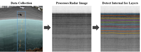
Fig. 1: Given an echogram from ground-penetrating radar over polar ice, we automatically estimate the number and position of internal ice layers. Left figure is adapted from [3].

Most automatic techniques for finding layers in these images only consider the ice-air and ice-bedrock boundaries, which are the most prominent [4, 5, 6, 7, 8]. A much more challenging problem is to identify the “internal” layers of the ice and snow caused by annual accumulation. At first glance, solving this problem may seem like a straightforward application of traditional computer vision techniques. However, approaches based on edge detection do not work well because the layer boundaries are subtle, the noise characteristics vary dramatically, and the number of visible layers changes across different regions of ice. Unlike most segmentation problems in computer vision, the layers here do not correspond to “objects” with distinctive colors or textures.

Nevertheless, our problem can be viewed as a generalization of the tiered scene segmentation problem [9]. Tiered segmentation partitions an image into a set of regions $\{r_{1},r_{2},...,r_{n}\}$ such that in each image column, all pixels belonging to $r_{i}$ are above (have lower row index than) all pixels corresponding to $r_{j}$ for $i<j$. Felzenswalb and Veksler [9] solved this problem using energy minimization with dynamic programming, but they assumed no more than three distinct labels per column because their inference time was exponential in the number of labels.

In this paper, we revisit tiered labeling using deep learning, and we consider a more challenging problem in which the number of labels is large and unknown ahead of time. We propose a novel deep neural network which performs the tiered segmentation in two stages. We first use a 2D convolutional network (CNN) to simultaneously solve three problems: detecting the position of the top layer, roughly estimating the average layer thickness, and estimating the number of visible layers. Propagating the estimated first layer downward using the estimated thickness gives a rough approximation of the tiered segmentation. Then we refine the pixel-level boundary positions using a recurrent neural network (RNN) to account for differences across different layers. We evaluate our method on internal ice layer segmentation on a large-scale, publicly-available polar echogram dataset. Experimental results show that our approach significantly outperforms baseline methods, and is especially efficient on multi-layer detection. Beyond polar ice, our technique is general and can be applied to tiered segmentation problems in other domains.

2 Related Work

Crandall et al. [4] detected two specific types of layer boundaries (ice-air and ice-bed) in echograms using discrete energy minimization with a pretrained template model and a smoothness prior. Lee et al. [5] proposed a more accurate method using Gibbs sampling from a joint distribution over all candidate layers, while Carrer and Bruzzone [10] further reduced the computational cost with a divide-and-conquer strategy. Xu et al. [6] extended the work to estimate 3D ice surfaces using a Markov Random Field (MRF), and Berger et al. [11] followed up with better cost functions that incorporate domain-specific priors. More recent work has applied deep learning. Kamangir et al. [8] detected ice boundaries using convolutional neural networks applied to wavelet features. Xu et al. [7] proposed a multi-task spatiotemporal neural network to reconstruct 3D ice surfaces from sequences of tomographic images. However, all of this work focuses on detecting a small, known number of layer boundaries (typically two) and thus is not appropriate for internal layers, because the number of visible internal layers varies and may be quite large.

Very recent work, contemporaneous to ours, has considered the internal layer detection problem. Varshney et al. [12] treat the problem as semantic segmentation, while Yari et al. [13] classify pixels into layer boundaries or not, which is a binary classification problem. Those papers require post-processing steps either to smooth the inconsistent labels between layers or to specify the layer indices.

Our problem can be thought of as a more general version of the tiered segmentation problem [9] proposed by Felzenswalb and Veksler, who presented an algorithm based on dynamic programming. However, their solution required the number of tiers (labels) to be fixed ahead of time to a small number (3) because their inference was exact and exponential in the number of labels, and used hand-crafted features. In this paper, we propose a new approach to a more general version of the tiered segmentation problem, in which the number of labels can be large and unknown. Our technique combines convolutional and recurrent neural networks for counting and detecting an arbitrary number of layer boundaries.

3 Methodology

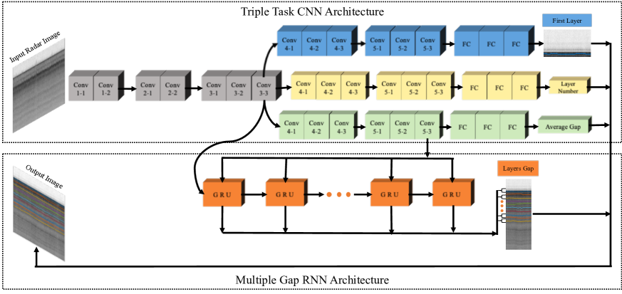
Fig. 2: Architecture of our model for detecting internal ice layers in radar echogram images. Through a combination of CNN and RNN networks, we estimate both the number of layers and the boundaries of each layer.

Given a noisy radar echogram $I$, which is a 2D image of size $1\times H\times W$ pixels, our goal is to localize $N$ internal ice layer boundaries and exactly one surface boundary between the ice and air. The output thus should be $N+1$ boundaries. We need to estimate both the number of boundaries $N$ (which varies from image to image, although our implementation assumes $N<30$) and all the boundary locations based on noisy and ambiguous data.

Our technique encodes the physical constraints of this tiered segmentation problem. First, since the labeled regions correspond to physical layers, layer boundaries cannot cross; more precisely, we partition the image into regions $\{r_{1},r_{2},...,r_{n}\}$ such that in each image column, all pixels belonging to $r_{i}$ are above all pixels corresponding to $r_{j}$ for $i<j$. Second, we assume that adjacent boundaries are roughly parallel, which is reasonable since the amount of snow or ice that falls in any given year is roughly consistent across local spatial locations. Finally, we assume that the thickness of different layers is roughly the same at any given spatial location, which is reasonable since the amount of snow or ice is similar across different years. These are all rough, weak assumptions, and our model is able to handle the significant deviations from them that occur in real radar data.

We address this problem using two main steps, following the intuition that a human annotator might use: first do a rough top-down segmentation of the image to incorporate global constraints on the layer structure, and then use that rough segmention to do a bottom-up refinement of the layer boundaries. More specifically, we first design a triple-task Convolutional Neural Network (CNN) model to estimate the number of ice layers $\hat{N}$, the location of the top layer $\hat{F}$ (encoded as a $W$-d vector indicating the row index for each column of the image), and the average thickness of all layers (the average vertical gap between boundaries) in the echogram. The top boundary is typically quite prominent since it is between air and ice, and provides a strong prior on the shape of the much weaker boundaries below. Second, we design a Recurrent Neural Network (RNN) to estimate $\hat{GapM}$, an $N\times W$ matrix encoding the thickness (gap between adjacent boundaries) for each layer at each column, based on the estimates in the first step.

To generate the final segmentation, we combine $\hat{F}$ and $\hat{GapM}$ according to $\hat{N}$ to generate output $\hat{M}$ which is a $(N+1)\times W$ matrix. Each element in $\hat{M}$ indicates the row index for a given boundary at a given column in the input $I$.

3.1 Triple Task CNN (CNN3B)

Our first step applies a three-branch Convolutional Neural Network (CNN) to roughly estimate the surface boundary location, the number of layer boundaries, and the average thickness of each internal layer across the echogram. Fig. 2 shows our CNN architecture, which was inspired by Xu et al. [7] but with significant modifications. Our model takes a 2D image $I$ as input. Then we use three shared convolutional blocks, each of which is followed by max pooling operations. The shared convolutional blocks are used to extract low-level features for the next three branches, because similar evidence is useful for estimating the first layer, the number of layers, and the average thickness.

The model then divides into three branches. The first branch estimates the position of the surface layer, and uses six convolutional layers for modeling features specific to the first layer and one fully connected layer to generate outputs $\hat{F}=\{\hat{f_{1}},\hat{f_{2}},\cdots,\hat{f_{W}}\}$. Each element represents the row coordinate of the first layer within that column. The ground truth vector $F=\{f_{1},f_{2},\cdots,f_{W}\}$ is generated from the top boundary of the human-labeled ground truth $M_{N}=\{m_{N,1},m_{N,2},\cdots,m_{N,W}\}$. The loss function for estimating the first layer uses an L1 Manhattan distance to encourage the model’s output to agree with the human-labeled ground truth,

$$L_{fl}=\frac{1}{W}\sum_{w=1}^{W}\left|\hat{f}_{w}-f_{w}\right|.$$ (1)

The second branch predicts the number of ice layer boundarise, and includes six convolutional layers and three fully connected layers. We view this as a classification problem, so this branch produces a vector $v$ which is a probability distribution over a discrete set of possible numbers of boundaries. In our experiments, we assume $N<30$, so $v$ is 31-dimensional. The ground truth is the number of labeled boundaries $N$ in the human-annotated ground truth of the image. Cross-entropy loss is used during training,

$$L_{number}=-\log\left(\frac{\exp(v[\operatorname{N}])}{\sum_{j}\exp(v[j])}\right).$$ (2)

The third branch roughly estimates the average thickness (gap) of all the layers in the echogram, and follows the same general design as the first branch but with a single scalar output from the final fully connected layer. The loss calculates the absolute value between the output $\hat{\Delta}$ and the ground truth $\Delta$,

$$L_{\Delta}=\left|\hat{\Delta}-\Delta\right|.$$ (3)

Finally, our CNN loss function combines the three branches,

$$L=L_{fl}+L_{number}+L_{\Delta}.$$ (4)

We use VGG16 [14] as the network backbone.

3.2 Multiple Gap RNN

Having roughly estimated the global structure of the echogram in the last section, we next use an RNN to generate a more accurate gap (thickness) value for each layer in the echogram. We use Gated Recurrent Units (GRUs) [15], which require less computational cost and are easier to train than LSTMs [16].

As shown in Fig. 2, our model has one hidden layer, wherein each GRU cell takes feature map $Avg_{F}$ generated before the fully connected layer of our Triple Task CNN model’s third branch and the output of the previous GRU cell as inputs, and produces $W$ real-valued numbers indicating the predicted gap between layer boundaries within each column of the data. $Avg_{F}$ is projected to the size of the GRU hidden state with a fully connected layer before GRU takes it as input. During training, the GRU cell is operated for $N$ iterations, where each iteration $n$ estimates the gap between layer $n+1$ and layer $n$. In a given iteration $n$, the GRU cell takes the projected $Avg_{F}$ as input. The GRU cell outputs a sequence of hidden states $\{h_{1},h_{1},\cdots,h_{n}\}$ with iteration $n\in[1,N]$, and each hidden state $h_{n}$ is followed by a fully-connected layer to predict gap value $\hat{GapM_{n}}$. We use L1 Manhattan distance to supervise the model to predict $\hat{GapM}$ according to the human-labeled ground truth $GapM$,

$$L_{GapM}=\frac{1}{N}\frac{1}{W}\sum_{n=1}^{N}\sum_{w=1}^{W}\left|\hat{GapM_{n,w}}-GapM_{n,w}\right|.$$ (5)

3.3 Combination

We combine our Triple Task CNN and Multiple Gap RNN to predict the number of internal ice layer boundaries and their positions in the input image $I$. The RNN uses general features as shown in Fig. 2 to initialize the GRU’s hidden state and takes an average feature map $Avg_{F}$ as input. Based on the first layer output and the number of layers from the Triple Task CNN, our model generates the first boundary $M_{0}$ ($W$-d vector) in our result $\hat{M}$. We then apply the layer gap output $GapM$ predicted by our multiple Gap RNN according to the first layer result,

$$\begin{array}[]{c}M_{i}=M_{i-1}+GapM_{i},i\in(1,N),\end{array}$$ (6)

where N is number of layer boundaries. In addition, $M_{i}$ and $GapM_{i}$ are both $W$-d vectors. For each image, we compute all $M_{i}$’s to create $\hat{M}$ which is a $(N+1,W)$ matrix, and compare it with ground truth $M$ to evaluate our model.

4 Experiments

4.1 Dataset

We use the annual ice layer dataset collected by the Center for Remote Sensing of Ice Sheets (CReSIS) at the University of Kansas and the National Snow and Ice Data Center at the University of Colorado [17]. The data is collected by ultra-wideband snow radar operated over a frequency range from 2.0 to 6.5 GHZ, and consists of 17,529 radar images with human-labeled annotations that identify the positions of internal ice layers. Formally, our task is to detect all internal ice layers $\hat{M}$ in a given single-channel image $I$. Each element in $\hat{M}$ indicates the row coordinate (in the range $[1,H]$, where $H$ is image height) of an ice layer for a given column.

Preprocessing. We resize all input images to $300\times 256$ by using bi-cubic interpolation. We normalize the grayscale pixel values by subtracting the mean and dividing by the standard deviation (both of which are calculated from the training data). Following [7], we also normalize the ground truth row labels to a coordinate system spanning $[-1,1]$ in each image. We also remove input images that have missing data.

4.2 Implementation Details

We use PyTorch to implement our model and do the training and all experiments on a system with Pascal Nvidia Titan X graphics card. We randomly choose 80% of images for training and 20% for testing. The Adam optimizer with default parameters is used to learn the CNN parameters with batch size of 16. The training process is stopped after 30 epochs, starting with a learning rate of $10^{-4}$ and reducing in half every 10 epochs. The RNN training uses the same optimizer, update rule, and batch size as the CNN’s, but initial learning rate is set to $10^{-3}$.

4.3 Evaluation Metrics

Prior work has used mean absolute error in pixels between predicted and ground truth layers [4, 5], a familiar evaluation metric in signal processing applications. However, in our problem of internal ice detection, the number of layers is unknown, which means the evaluation metric must capture both the accuracy of estimated layer count and the localization accuracy of the layers. Prior work on internal layer detection has typically been evaluated qualitatively [18].

We thus introduce two quantitative, objective evaluation approaches for the tiered segmentation problem. Our first evaluation protocol assumes that the correct number of layers is known via an oracle, and then measures mean absolute error in pixels. Assuming that the correct number of layers is given is useful both for isolating the accuracy of layer localization, and for allowing comparison with models that are not able to estimate layer counts. To evaluate the accuracy of both the layer count and layer boundaries, we propose layer-AP based on average precision. For each estimated layer, we search through the ground truth layers to find the closest match according to mean absolute error. Each ground truth layer is only allowed to match one estimated layer. Then we define a set of threshold values $t_{l}$. For each threshold, we count the number of estimated layers which have a mean absolute error in pixels under the threshold, and call this the number of matches $m_{i}$ for that threshold. In particular, the layer average precision is computed as,

$$\textrm{layer-AP}=\frac{1}{l}\sum_{i=1}^{l}\frac{m_{i}}{N+1},$$ (7)

where $N+1$ is the number of layer boundaries ($N$ is the number of gaps between boundaries), and $l$ indicates the number of thresholds. In this work, we use 10 different thresholds and set $t_{l}=[1,4,7,10,13,16,19,22,25,27]$, assuming input images are in size of $300\times 256$.

4.4 Baselines

We are not aware of any existing work that solves the problem we consider here: existing fully-automatic approaches to the tiered segmentation problem assume the number of layers is no greater than two and is known ahead of time. We thus develop some baseline models to compare our results against.

Crandall et al. [4] proposed a technique based on graphical models to find layer boundaries, which we call Sequential. However, they assume exactly two layer boundaries because the running time is exponential in the number of layers. Here, we adapted it to our problem by using an oracle to determine the number of layers (by looking at ground truth), and then running sequentially to find each layer one-by-one. Naive CNN uses the VGG16 [14] as backbone which directly predicts a fixed number of internal layers by producing a label matrix in one-shot. RNN30 models the dependencies in the vertical direction: given the estimated boundary for a given layer and previous layers, it predicts the boundary for the subsequent (next-deeper) annual layer. RNN256 is a baseline that uses a recurrent neural network (RNN) to model sequential dependencies across columns, assuming a fixed number of layers. CNN2B is a simpler version of our model that uses only two branches, one to predict the top layer (the air and ice boundary), and one to predict the average gap between layers. CNN3B is a version of our model with all three branches, but without the RNN refinement. CNN3B+RNN is our full model described above.

4.5 Evaluation Results

Quantitative results are presented in Table 1 and 2 in terms of mean absolute error and layer-AP, respectively. In each table, we present two sets of results: one in which the number of layers is known ahead of time by an oracle (i.e., by consulting the ground truth), and one in which it is predicted automatically. Note that only the techniques that use CNN3B are able to estimate the number of layers automatically, which is why the other results are listed as missing in the table. For calculating mean absolute error when models incorrectly estimate the number of layers, we pad either the ground truth or the output (whichever has fewer layers) with extra layers consisting of zero vectors to penalize these incorrect estimations.

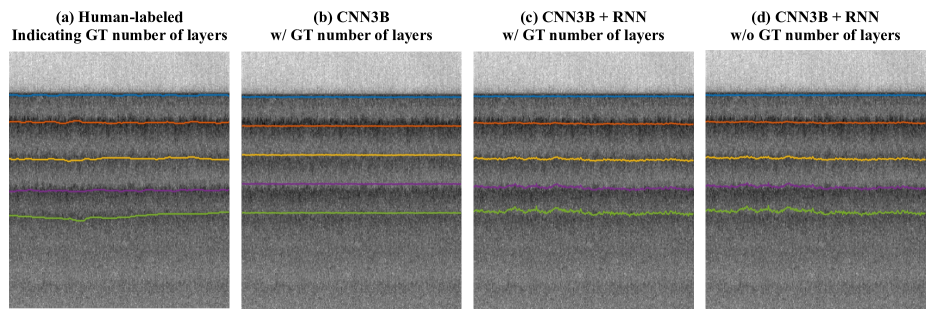
Fig. 3: Sample results, showing (a) ground truth, (b) CNN3B output with ground truth number of layers, (c) CNN3B+RNN with ground truth number of layers, and (d) CNN3B+RNN with estimated number of layers.

Comparing with other models in Table 1 and 2, we observe that our combination of CNN3B and RNN models significantly outperforms all baselines in terms of both mean average error and layer-AP. Our two models CNN3B and CNN3B+RNN have the ability to estimate the number of internal ice layers, and reach $85.2\%$ accuracy on this layer counting task, which is why their accuracy decreases only slightly when the number of layers is not provided by the oracle. Our model CNN3B+RNN shows the best results of all other baselines, even when our model must estimate the number of layers and the the baselines know it from the oracle.

	Mean Error (in pixels) $\downarrow$
	# layers from oracle	# layers estimated
Sequential [4]	88.98	-
Naive CNN	24.32	-
RNN30	21.79	-
RNN256	20.20	-
CNN2B	11.94	-
CNN3B	7.91	9.27
CNN3B+RNN	6.96	8.73

Table 1: Evaluation results by measuring the error in terms of the mean absolute column-wise difference compared to ground truth, in pixels.

	layer-AP $\uparrow$
	# layers from oracle	# layers estimated
Sequential [4]	0.059	-
Naive CNN	0.183	-
RNN30	0.218	-
RNN256	0.254	-
CNN2B	0.635	-
CNN3B	0.843	0.822
CNN3B+RNN	0.882	0.853

Table 2: Evaluation results by measuring the layer average precision with thresholds compared to ground truth.

Qualitative results are shown in Fig. 3. The first column shows the human annotated layers, while the second column shows the result generated by one of our baselines, CNN3B. The results of this baseline roughly agree with the ground truth, but all layers except the first show different degrees of inaccurate localization compared with the human annotations. The third and fourth columns show the results with and without the layer number oracle. Since our CNN3B+RNN model is highly accurate at estimating the number of layers, the output with and without the oracle are nearly the same. We provide additional sample results in supplementary material.

As shown in the examples, our model only needs the input image to generate results that are very close to human annotations in most cases. The improvement between CNN3B and CNN3B+RNN indicates that the RNN contributes to our final result even though the RNN30 and RNN256 baselines fail to work well on their own. The results show that both steps of our model are important to achieve high performance.

5 Conclusion

We have considered a generalization of the tiered segmentation problem and apply it to a problem of great societal consequence: automatically understanding the internal layer structure of the polar ice sheets from ground-penetrating radar echograms. We show that our approach can effectively estimate arbitrary numbers of snow or ice layers from noisy radar images. Experimental results on a challenging, publicly-available dataset demonstrate the significant improvements over existing methods.

6 Acknowledgments

This work was supported in part by the National Science Foundation (DIBBs 1443054, CAREER IIS-1253549), and by the IU Office of the Vice Provost for Research, the IU College of Arts and Sciences, and the IU Luddy School of Informatics, Computing, and Engineering through the Emerging Areas of Research Project “Learning: Brains, Machines, and Children.” We acknowledge the use of data from CReSIS with support from the University of Kansas and Operation IceBridge (NNX16AH54G).

7 More Experiment Results

Fig. 4 shows two more examples with different numbers of internal layers. In each example, the first column shows the human annotated layers with input data as background. The second column shows the estimated result generated by one of our baselines, CNN3B. The results of this baseline roughly agree with the ground truth, but have some clear defects. For example, in the first row, the second orange layer in the CNN3B result fails to match the ground truth well. In the second row, the third yellow layer and fourth purple layer show clear mismatches. The third and fourth columns show the prediction result with and without the layer number oracle. Since our CNN3B+RNN model successfully predicts the number of layers in these three cases, the output with and without the oracle are nearly the same. Both our CNN3B+RNN results show improvements in both cases. In the first row, the second orange layer matches the human annotation in the first column better than CNN3B in the second column. In the second row, the third yellow layer and fourth purple layer are clearly closer to the ground truth than the result.

There are two failure cases showed in Fig. 5. In the fist failure case, there are 6 internal layers in the ground truth, but CNN3B+RNN without the oracle fails to predict the number of layers correctly. Our CNN3B only predicts the first layer well and shows a clear mismatch in all the other layers, but our CNN3B+RNN result in the fourth column predicts the first 5 layers reasonably well. Our CNN3B+RNN with the oracle shows the best results for this case, but there are still many ripples in the result showing that our model failed to predict it perfectly. In the second failure case, our CNN3B model fails to predict almost all the layers, while CNN3B+RNN both fails to estimate the number of layers or match most of the internal layers. However, CNN3B+RNN still works well for the first two layers.

There are two causes for these failure cases. First, the input data is noisy and complex, and difficult to be annotated even by an experienced human annotator. Not only does this means that our model must learn to process the complex and noisy input data, but it also means that the “ground truth” from human annotators also has much noise and inconsistency. This annotation noise not only adds noise during training, but also means that we are measuring error against ground truth that in itself has many errors. Second, we face a significant unbalanced dataset issue: there only 1.35% of the images have more than 5 internal ice layers, for example, which may affect our model’s learning capability.

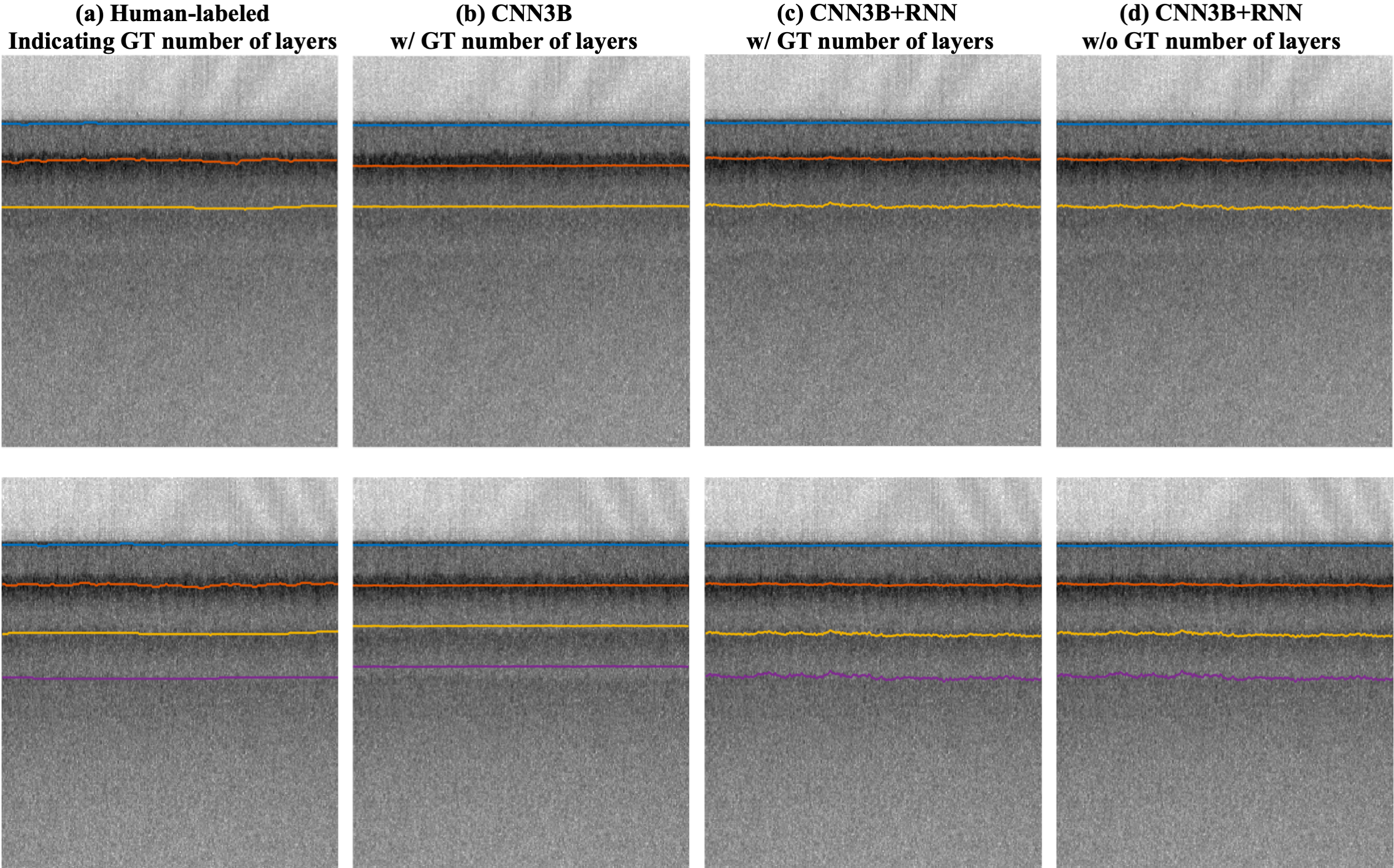
Fig. 4: Sample results. First column is input data with ground truth. Second column is one of our baselines, CNN3B, with ground truth number of layers. Third column is our best model, CNN3B+RNN, with ground truth number of layers. Fourth column is our best model, CNN3B+RNN, with estimated number of layers.

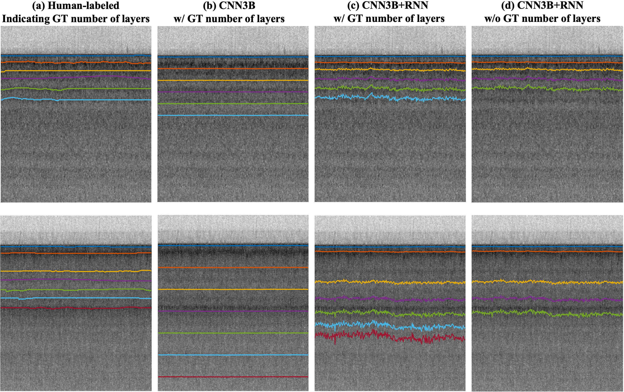
Fig. 5: Failure cases. First column is input data with ground truth. Second column is one of our baseline CNN3B result with ground truth number of layers. Third column is our best model CNN3B+RNN result with ground truth number of layers. Fourth column is our best model CNN3B+RNN result with prediction number of layers. Two rows represent two different input data with annotations and prediction results.

References

- [1] J. Houghton, Global warming: The complete briefing, Cambridge University Press, 2009.
- [2] J. MacGregor et al., “Radiostratigraphy and age structure of the Greenland Ice Sheet,” J. Geophys. Res. Earth Surf., 2015.
- [3] Climate Central, “New 3D Age Map of the Greenland Ice Sheet,” https://www.youtube.com/watch?v=T29_6Za3k2M, 2015.
- [4] D. Crandall, G. Fox, and J. Paden, “Layer-finding in radar echograms using probabilistic graphical models,” in ICPR, 2012.
- [5] S. Lee, J. Mitchell, D. Crandall, and G. Fox, “Estimating bedrock and surface layer boundaries and confidence intervals in ice sheet radar imagery using MCMC,” in ICIP, 2014.
- [6] M. Xu, D. Crandall, G. Fox, and J. Paden, “Automatic estimation of ice bottom surfaces from radar imagery,” in ICIP, 2017.
- [7] M. Xu, C. Fan, J. Paden, G. Fox, and D. Crandall, “Multi-task spatiotemporal neural networks for structured surface reconstruction,” in WACV, 2018.
- [8] H. Kamangir, M. Rahnemoonfar, D. Dobbs, J. Paden, and G. Fox, “Deep hybrid wavelet network for ice boundary detection in radar imagery,” in IGARSS, 2018.
- [9] P. Felzenszwalb and O. Veksler, “Tiered scene labeling with dynamic programming,” in CVPR, 2010.
- [10] L. Carrer and L. Bruzzone, “Automatic enhancement and detection of layering in radar sounder data based on a local scale hidden Markov model and the Viterbi algorithm,” IGRASS, 2017.
- [11] V. Berger, M. Xu, S. Chu, D. Crandall, J. Paden, and G. Fox, “Automated Tracking of 2D and 3D Ice Radar Imagery Using Viterbi and TRW-S,” in IGARSS, 2018.
- [12] D. Varshney, M. Rahnemoonfar, M. Yari, and J. Paden, “Deep ice layer tracking and thickness estimation using fully convolutional networks,” in Big Data, 2020.
- [13] M. Yari, M. Rahnemoonfar, J. Paden, L Koenig, and I. Oluwanisola, “Multi-scale and temporal transfer learning for automatic tracking of internal ice layers,” in IGARSS, 2020.
- [14] K. Simonyan and A. Zisserman, “Very deep convolutional networks for large-scale image recognition,” ICLR, 2015.
- [15] J. Chung, C. Gulcehre, K. Cho, and Y. Bengio, “Gated feedback recurrent neural networks,” in ICML, 2015.
- [16] S. Hochreiter and J.S chmidhuber, “Long short-term memory,” Neural computation, 1997.
- [17] L. Koenig et al., “Annual greenland accumulation rates from airborne snow radar,” The Cryosphere, 2016.
- [18] J. Mitchell, D. Crandall, G. Fox, and J. Paden, “A semi-automatic approach for estimating near surface internal layers from snow radar imagery,” in IGARSS, 2013.