Differentially Private Deep Learning with Direct Feedback Alignment

Abstract

Standard methods for differentially private training of deep neural networks replace back-propagated mini-batch gradients with biased and noisy approximations to the gradient. These modifications to training often result in a privacy-preserving model that is significantly less accurate than its non-private counterpart.

We hypothesize that alternative training algorithms may be more amenable to differential privacy. Specifically, we examine the suitability of direct feedback alignment (DFA). We propose the first differentially private method for training deep neural networks with DFA and show that it achieves significant gains in accuracy (often by 10-20%) compared to backprop-based differentially private training on a variety of architectures (fully connected, convolutional) and datasets.

1 Introduction

An unanswered question, with significant implications, is what is the best way to train deep networks with differential privacy. The non-private setting has seen rapid advances in the state-of-the-art while progress in the privacy-preserving setting has been lagging. Currently there are two promising privacy-preserving approaches, each with its own drawbacks. (1) Knowledge distillation approaches, such as PATE [27, 28], requires massive quantities of public data (i.e., data that will not receive privacy protections) in addition to massive amounts of sensitive data (which will be protected). These requirements limit their applicability. (2) Adaptations of stochastic gradient descent [1, 37, 3, 32, 23, 10, 9, 2], are more widely applicable but result in low accuracy compared to non-private models. They operate by separately clipping the gradient for each example in a batch before aggregating — that is, they clip then aggregate, instead of using the aggregate-then-clip approach common in non-private training [14]. Noise is added to the gradient estimate and then parameters are updated. The result is a biased and noisy gradient that causes final model accuracy to deteriorate [7].

In this paper, we focus on the setting where the entire dataset is sensitive and we seek alternatives to differentially private stochastic gradient descent. Specifically, we consider the suitability of direct feedback alignment (DFA) [26] for privacy-preserving training of artificial neural networks. DFA is a biologically inspired alternative to backprop/SGD that is much more suitable for low-power hardware [16, 11]. We propose the first differentially private algorithm for DFA. A careful analysis shows privacy can be achieved by (i) clipping the activations and error signal after (not during) the feed-forward phase, (ii) carefully choosing the error transport matrix, and (iii) adding Gaussian noise to the update direction.

Empirical results on a variety of datasets show the following results. (1) Differentially private DFA outperforms (by a wide margin) differentially private SGD on fully connected networks with various activation functions. (2) Networks with fully connected layers stacked on top of convolutional layers benefit significantly from a hybrid approach that combines DFA at the top layers with SGD at the bottom layers (mirroring an earlier result in the non-private setting [16]).

2 Related Work

Backpropagation (BP) [30] and stochastic gradient descent (SGD) have been essential tools for training modern deep learning models in both non-private and private settings. In some communities, such as cognitive neuroscience, debates about biological implausibility of BP (e.g., weight transport problem [15, 20, 4]) motivated approaches such as feedback alignment (FA) [21], direct feedback alignment (DFA) [26], and difference target propagation (DTP) [19], which introduce new learning mechanisms for error feedback signals. Recent work [8, 25, 11] found that biologically plausible learning algorithms generally underperform BP on convolutional neural networks, but hybrid DFA/BP approaches can work well [16].

The first differentially private training algorithm for deep learning models was proposed by Shokri and Shmatikov [31]. It relied on a distributed system in which participants jointly train a model by exchanging perturbed SGD updates. However, it incurred a privacy cost that was too large to be practical (e.g., $\epsilon$ values in the hundreds or thousands). Abadi et al. [1] proposed a training algorithm that satisfied Renyi Differential Privacy [24], which allowed training of networks with more practical privacy costs (epsilon values in the single digits). It modified SGD by individually clipping the gradient of each example before aggregating them into batches, then adding appropriately-scaled Gaussian noise, and then updating parameters as in standard SGD. This per-example-gradient clipping was designed to control the influence of any single data point. They also introduced a moment accountant to keep track of privacy protections due to Gaussian noise and subsampling (in the selection of batches). Their method has generated substantial interest, and follow-up research [37, 3, 32, 23, 22, 10, 9, 2] investigated additional architectures and efficient clipping strategies. Clipping gradients before aggregating them in batches is known to produce bias — the estimated mini-batch gradient no longer points in the same direction as the true mini-batch gradient. As we show experimentally, this bias already causes a degradation in model accuracy (even without noise addition).

In some special cases, gradient clipping can be avoided. Phan et al. [29] focused on learning auto-encoders by perturbing the objective function. Xie et al. [35] showed that a differentially private Wasserstein GAN [6] can be trained by clipping weights instead of gradients. PATE [27, 28] also avoids gradient clipping, but requires a large non-sensitive dataset in order to operate.

To the best of our knowledge, we propose the first differentially private version of direct feedback alignment.

3 Preliminaries

We next introduce our notation and provide background on DFA and (Renyi) Differential privacy.

3.1 Notation

We use bold-face uppercase letters (e.g., ${\bm{\mathrm{W}}}$) to represent matrices, bold-face lowercase letters (e.g., $\mathbf{x}$) to represent vectors and non-bold lowercase letters (e.g., $y$) to represent scalars. Tensors of order 3 or higher (i.e., multidimensional arrays indexed by 3 or more variables) are represented in calligraphic font (e.g,. $\mathcal{W}$). We index vectors using square brackets (e.g., $\mathbf{x}[1]$ is the first component of the vector $\mathbf{x}$). For matrices, we use subscripts to identify entries ($W_{i,j}$ is the entry in row $i$, column $j$).

We use the following notation to represent a dataset $D$ and its constituent records: $D=\{\bm{\mathrm{d}}_{i}=(\bm{\mathrm{x}}_{i},\bm{\mathrm{y}}_{i})\}_{i=1}^{n}$ is a set of $n$ examples, where $\textbf{x}_{i}$ is a feature vector (e.g., image pixels) and $\bm{\mathrm{y}}_{i}$ is a one-hot encoded target vector (i.e., to represent class $k$, $\bm{\mathrm{y}}_{i}[k]=1$ and all other components are 0).

(a) BP

(b) DFA

(c) Hybrid BP/DFA for Convolutional Neural Networks

Figure 1: Comparison of different error transportation configurations

3.2 Backpropagation and DFA

Direct Feedback Alignment [26] is best explained by showing how it deviates from backprop.

As an example, consider a feed-forward network $f_{\theta}$, consisting of $L$ fully-connected layers with a soft-max output (for a classification task). Let ${\bm{\mathrm{W}}}^{l}\in\mathbb{R}^{n_{l}\times n_{l-1}}$ and $\bm{\mathrm{b}}^{l}\in\mathbb{R}^{n_{l}}$ denote the weight and bias of the $l$^th layer in $f_{\theta}$, respectively. The feed-forward step of layer is defined by:

$$\bm{\mathrm{h}}^{l}=\phi_{l}(\bm{\mathrm{z}}^{l})\,,\quad\bm{\mathrm{z}}^{l}={\bm{\mathrm{W}}}^{l}\bm{\mathrm{h}}^{l-1}+\bm{\mathrm{b}}^{l}\,,\quad\theta=\{({\bm{\mathrm{W}}}^{l},\bm{\mathrm{b}}^{l})\}_{l=1}^{L}\,,$$ (1)

where $\bm{\mathrm{z}}^{l}\in\mathbb{R}^{n_{l}}$ is the pre-activation and $\bm{\mathrm{h}}^{l}\in\mathbb{R}^{n_{l}}$ is the (post-) activation of the layer obtained by applying the activation function $\phi_{l}$ element-wise on $\bm{\mathrm{z}}^{l}$. In our notation, $\bm{\mathrm{h}}^{0}=\bm{\mathrm{x}}$ denotes the input record. In the final layer (with softmax activation), the $k$^th output is $\bm{\mathrm{h}}^{L}[k]=\frac{\exp(\bm{\mathrm{z}}^{L}[k])}{\sum_{j}\exp(\bm{\mathrm{z}}^{L}[j])}$, which can be interpreted as the probability estimate for class $k$. Continuing our example, suppose the network is to be trained with cross-entropy loss. That is, if $f_{\theta}(\bm{\mathrm{x}})\equiv\hat{\bm{\mathrm{y}}}$ is the output vector for input $\bm{\mathrm{x}}$ with true class label $\bm{\mathrm{y}}$, the cross-entropy loss for that record is $\mathcal{L}(\bm{\mathrm{h}}^{L})=-\sum_{k}\bm{\mathrm{y}}[k]\log\hat{\bm{\mathrm{y}}}[k]$.

In BP, the gradient of $\mathcal{L}$ w.r.t. the parameter ${\bm{\mathrm{W}}}^{l}$ is computed using the chain rule and updated as follows:

$$\delta\bm{\mathrm{z}}^{l} =\frac{\partial\bm{\mathrm{h}}^{l}}{\partial\bm{\mathrm{z}}^{l}}\frac{\partial\bm{\mathrm{z}}^{l+1}}{\partial\bm{\mathrm{h}}^{l}}\frac{\partial L}{\partial\bm{\mathrm{z}}^{l+1}}=\begin{cases}\left(({\bm{\mathrm{W}}}^{l+1})^{\intercal}\delta\bm{\mathrm{z}}^{l+1}\right)\odot\phi_{l}^{\prime}(\bm{\mathrm{z}}^{l})&\mbox{ if $l<L$,}\\ \hat{\bm{\mathrm{y}}}-\bm{\mathrm{y}}&\mbox{ if $l=L$,}\end{cases}$$ (2)

$$\frac{\partial\mathcal{L}}{\partial{\bm{\mathrm{W}}}^{l}} =\frac{\partial\bm{\mathrm{z}}^{l}}{\partial{\bm{\mathrm{W}}}^{l}}\frac{\partial L}{\partial\bm{\mathrm{z}}^{l}}=\delta\bm{\mathrm{z}}^{l}(\bm{\mathrm{h}}^{l-1})^{\intercal}$$ (3)

$${\bm{\mathrm{W}}}^{l} \leftarrow{\bm{\mathrm{W}}}^{l}-\eta\frac{\partial\mathcal{L}}{\partial{\bm{\mathrm{W}}}^{l}};\quad\bm{\mathrm{b}}^{l}\leftarrow\bm{\mathrm{b}}^{l}-\eta\delta\bm{\mathrm{z}}^{l}$$ (4)

where $\eta$ is the step size, $\odot$ is an element-wise multiplication operator and $\phi^{\prime}_{l}$ denotes the derivative of the activation function. Equation (2) shows that the backward error signal $\delta\bm{\mathrm{z}}^{l}$ for layer $l$ is computed using the signal $\delta\bm{\mathrm{z}}^{l+1}$ propagated from the layer above. Starting from the output layer, the error information propagates backward through the network from layer to layer. Notice that the error signal $\delta\bm{\mathrm{z}}^{l}$ requires the transpose of forward weight matrix ${\bm{\mathrm{W}}}^{l+1}$. In other words, ${\bm{\mathrm{W}}}^{l+1}$ appears in both feed-forward and backward paths.

DFA makes two modifications to the backward path of BP (and only the backward path). First, for each layer, it replaces ${\bm{\mathrm{W}}}^{l+1}$ in the backward path with a random feedback weight matrix ${\bm{\mathrm{B}}}^{l+1}$ (chosen at the beginning of training). The entries of ${\bm{\mathrm{B}}}^{l+1}$ are randomly sampled from a probability distribution such as the Gaussian distribution and then are fixed throughout the training process (i.e. they do not get updated/learned). The second change introduced by DFA is that instead of propagating the error signal backward through the layers, the error signal at each layer depends directly on $\delta\bm{\mathrm{z}}^{L}$, which is the error signal of the output layer. Due to the special importance of $\delta\bm{\mathrm{z}}^{L}$, we denote this error signal by $\bm{\mathrm{e}}$ (which equals $\hat{\bm{\mathrm{y}}}-\bm{\mathrm{y}}$ for cross-entropy loss over softmax output). Mathematically, the error signal $\delta\bm{\mathrm{z}}^{l}$ at layer $l$ is:

$$\delta\bm{\mathrm{z}}^{l}=\left({\bm{\mathrm{B}}}^{l+1}\bm{\mathrm{e}}\right)\odot\phi_{l}^{\prime}(\bm{\mathrm{z}}^{l})\,.$$ (5)

Compared to Equation 2, $({\bm{\mathrm{W}}}^{l+1})^{\intercal}$ is replaced with ${\bm{\mathrm{B}}}^{l+1}$ while $\delta\bm{\mathrm{z}}^{l+1}$ is replaced with $\bm{\mathrm{e}}$. Plugging Equation 5 into Equation 3 and then 4, one arrives at the DFA update equation for ${\bm{\mathrm{W}}}^{l}$ (the weights used in the feed-forward pass) and $\bm{\mathrm{b}}^{l}$:

$${\bm{\mathrm{W}}}^{l}\leftarrow{\bm{\mathrm{W}}}^{l}-\eta\left(\left({\bm{\mathrm{B}}}^{l+1}\bm{\mathrm{e}}\right)\odot\phi^{\prime}(\bm{\mathrm{z}}^{l})\right)(\bm{\mathrm{h}}^{l-1})^{\intercal}\,;\quad\bm{\mathrm{b}}^{l}\leftarrow\bm{\mathrm{b}}^{l}-\eta\left(\left({\bm{\mathrm{B}}}^{l+1}\bm{\mathrm{e}}\right)\odot\phi^{\prime}(\bm{\mathrm{z}}^{l})\right)$$

Graphically, the distinction between BP and DFA is illustrated in Figures 1(a) and 1(b).

3.3 Differential Privacy

Differential privacy is a formal notion of privacy that provides strong privacy protection in sensitive data analysis. It bounds the influence that one record can have on the output of a randomized algorithm.

We say two datasets $D_{1}$ and $D_{2}$ are neighbors if $D_{1}$ can be obtained from $D_{2}$ by changing one record and write $D_{1}{\sim}D_{2}$ to denote this relationship.

Definition 1 (($\epsilon,\delta$)-DP [13, 12]).

Given privacy parameters $\epsilon\geq 0$, $\delta\geq 0$, a randomized mechanism (algorithm) $\mathcal{M}$ satisfies ($\epsilon,\delta$)-differential privacy if for every set $S\subseteq\operatorname{range}(\mathcal{M})$ and for all pairs of neighboring datasets $D_{1}{\sim}D_{2}$,

$$\Pr[\mathcal{M}(D_{1})\in S]\leq\exp(\epsilon)\Pr[\mathcal{M}(D_{2})\in S]+\delta\,.$$

The probability is only with respect to the randomness in $\mathcal{M}$.

In differentially private deep learning, a mechanism corresponds to the set of parameter updates from processing one minibatch. Since training involves many minibatch updates, it is important to accurately track the combined privacy leakage from all minibatches used. In this work, we use Rényi Differential Privacy (RDP) [24] to track privacy leakage. RDP uses its own parameters, but after training finishes, the RDP parameters can be converted to the $\epsilon,\delta$ parameters of Definition 1. RDP relies on the concept of Rényi divergence:

Definition 2 (Rényi Divergence).

Let $P_{1}$ and $P_{2}$ be probability distributions over a set $\Omega$ and let $\alpha\in(1,\infty)$. Rényi $\alpha$-divergence $\operatorname{\mathfrak{D}}_{\alpha}$ is defined as: $\operatorname{\mathfrak{D}}_{\alpha}(P_{1}\;\|\;P_{2})=\frac{1}{\alpha-1}\log(\operatorname{\mathbb{E}}_{x\sim P_{2}}\left[P_{1}(x)^{\alpha}P_{2}(x)^{-\alpha}\right])$.

Rényi differential privacy requires two parameters: a moment $\alpha$ and a parameter $\epsilon$ that bounds the moment.

Definition 3 ($(\alpha,\epsilon)$-RDP [24]).

Given a privacy parameter $\epsilon\geq 0$ and an $\alpha\in(1,\infty)$, a randomized mechanism $\mathcal{M}$ satisfies $(\alpha,\epsilon)$-Rényi differential privacy (RDP) if for all $D_{1}$ and $D_{2}$ that differ on the value of one record, $\operatorname{\mathfrak{D}}_{\alpha}(\mathcal{M}(D_{1})\;\|\;\mathcal{M}(D_{2}))\leq\epsilon\,.$

A simple way to achieve $(\alpha,\epsilon)$-RDP is to take a vector-valued deterministic function $f$ and add appropriately scaled Gaussian noise as follows. The scale of the noise depends on the sensitivity of $f$.

Definition 4 ($L_{2}$ sensitivity).

Let $L_{2}$ sensitivity of $f$, denoted by $\Delta_{f}$ is equal to $\sup_{D_{1}\sim D_{2}}||f(D_{1})-f(D_{2})||_{2}$, where the supremum is taken over all pairs of neighboring datasets.

Lemma 1 (Gaussian Mechanism [24]).

Let $f$ be a function. Let $\alpha>1$ and $\epsilon>0$. Let $M$ be the mechanism that, on input $D$, returns $f(D)+N(0,\sigma^{2}{\bm{\mathrm{I}}})$, where $\sigma^{2}=\frac{\alpha\Delta^{2}_{f}}{2\epsilon}$. Then $M$ satisfies $(\alpha,\epsilon)$-RDP.

The composition theorem of RDP states that if $M_{1},\dots,M_{k}$ are mechanisms and each $M_{i}$ satisfies $(\alpha,\epsilon_{i})$-RDP, then their combined privacy leakage satisfies $(\alpha,\sum_{i}\epsilon_{i})$-RDP [24]. The parameters of RDP can be converted into those of $(\epsilon,\delta)$-DP through the following conversion result [24].

Lemma 2 (Conversion to $(\epsilon,\delta)$-DP [24]).

If $\mathcal{M}$ satisfies $(\alpha,\epsilon)$-RDP, it satisfies $(\epsilon^{\prime},\delta^{\prime})$-differential privacy whenever $\epsilon^{\prime}\geq\epsilon+\frac{\log(1/\delta)}{\alpha-1}$ and $\delta^{\prime}\geq\delta$.

The following lemma states that the privacy guarantee of an $(\alpha,\epsilon)$-RDP mechanism $\mathcal{M}$ is amplified when it is applied on poisson subsampled data.

Lemma 3 (Subsampled Mechanism and Privacy Amplification for RDP [33]).

For a randomized mechanism $\mathcal{M}$ and a dataset $D$, define $\mathcal{M}\circ\mathfrak{S}_{q}$ as (i) sample a subset $B\subseteq D$ (with $q=|B|/|D|$), by sampling without replacement (ii) apply $\mathcal{M}$ on $B$. Then if $\mathcal{M}$ satisfies $(\alpha,\epsilon(\alpha))$-RDP with respect to $B$, $\mathcal{M}\circ\mathfrak{S}_{q}$ satisfies $(\alpha,\epsilon^{\prime}(\alpha))$-RDP with respect to $D$ for any integer $\alpha\geq 2$, where $\epsilon^{\prime}(\alpha)\leq\frac{1}{\alpha-1}\log\big{(}1+q^{2}{\binom{\alpha}{2}}\min\left\{4(e^{\epsilon(2)}-1),2e^{\epsilon(2)},e^{\epsilon(2)}(e^{\epsilon(\infty)}-1)^{2}\right\}+\sum_{l=3}^{\alpha}{\binom{\alpha}{l}}q^{l}e^{(l-1)\epsilon(l)}\min\{2,(e^{\epsilon(\infty)}-1)^{j}\}\big{)}$.

4 Differentially Private DFA

In this section, we propose a differentially private version of direct feedback alignment. Given a positive constant $c$, the clipping function shrinks the norm of a vector until it is at most $c$. Formally, $\mathsf{clip}_{c}(\bm{\mathrm{v}})=\min(c,\lVert\bm{\mathrm{v}}\rVert_{2})\frac{\bm{\mathrm{v}}}{\lVert\bm{\mathrm{v}}\rVert_{2}}\,.$ Our algorithm for privatizing DFA has several components: (1) first, we require that the (sub)derivatives of each activation function $\phi_{l}$ be bounded by a constant $\gamma_{l}$ (i.e., $|\phi_{l}^{\prime}(v)|\leq\gamma_{l}$ for all scalars $v$). This is true for the most commonly used activations such as ReLU, sigmoid, tanh, etc.; (2) then we construct the feedback matrices ${\bm{\mathrm{B}}}^{l}$ with spectral norm (largest singular value) equal to $\beta_{l}$ (an algorithm parameter); the entries of ${\bm{\mathrm{B}}}^{l}$ are sampled independently from the standard Gaussian distribution, and then this matrix is rescaled by a constant so that $||{\bm{\mathrm{B}}}^{l}||=\beta_{l}$; (3) we construct a mini-batch of size $m$ by sampling without replacement; (4) after the feed-forward phase completes, we compute the clipped version (with parameter $\tau_{h}$) of the post-activation $\bm{\mathrm{h}}_{l}$ of each layer and we also clip with parameter $\tau_{e}$ the error vector $\bm{\mathrm{e}}$; (5) we then add Gaussian noise to the DFA mini-batch update direction. The full algorithm is shown in Algorithm 1.

Input: A feed-forward network $f_{\theta}=\{({\bm{\mathrm{W}}}^{l},\bm{\mathrm{b}}^{l})\}_{l=1}^{L}$, upper bounds $\gamma_{l}$ on derivative of activation functions, spectral norm bounds $\beta_{l}$, clipping thresholds $\tau_{e},\tau_{h}$, stepsize $\eta$, noise scale $\sigma$, minibatch size $m$, number of iterations $T$.

1 for $l=1$ to $L$ do

     Intialize ${\bm{\mathrm{B}}}^{l}$,  then normalize: ${\bm{\mathrm{B}}}^{l}=\beta_{l}{\bm{\mathrm{B}}}^{l}/\lVert{\bm{\mathrm{B}}}^{l}\rVert_{2}$

       // spectral normalization

2     

3      end for

4     for $T$ iterations do

5          Create a minibatch of size $m$ by sampling without replacement

6           $S\leftarrow$ indices of records in the mini-batch

7           for $i$ in $S$ do

8                for layer $l=1$ to $L-1$ do // feed-forward phase

                    $\bm{\mathrm{z}}^{l}_{i}={\bm{\mathrm{W}}}^{l}\bm{\mathrm{h}}_{i}^{l-1}+\bm{\mathrm{b}}^{l}$;  $\bm{\mathrm{h}}_{i}^{l}=\phi_{l}(\bm{\mathrm{z}}_{i}^{l})$; 

                      // process record $i$

9                    

10                     end for

11                    $\hat{\bm{\mathrm{y}}}_{i}\leftarrow\mathsf{softmax}({\bm{\mathrm{W}}}^{L}\bm{\mathrm{h}}_{i}^{L-1}+\bm{\mathrm{b}}^{L})$

                     $\bm{\mathrm{e}}_{i}=\mathsf{clip}_{\tau_{e}}(\hat{\bm{\mathrm{y}}}_{i}-\bm{\mathrm{y}}_{i})$

                      // error clipping

12                    

13                     end for

14                    for $l=L$ to $1$ do // activation clipping and parameter updates

15                         ${\bm{\mathrm{W}}}^{l}\leftarrow{\bm{\mathrm{W}}}^{l}-\eta\left(\mathcal{N}(0,\sigma^{2}{\bm{\mathrm{I}}})+\frac{1}{m}\sum_{i\in S}\left(({\bm{\mathrm{B}}}^{l+1}\bm{\mathrm{e}}_{i})\odot\phi^{\prime}_{l}(\bm{\mathrm{z}}_{i}^{l})\right)\mathsf{clip}_{\tau_{h}}(\bm{\mathrm{h}}_{i}^{l-1})^{\intercal}\right)$

16                          $\bm{\mathrm{b}}^{l}\leftarrow\bm{\mathrm{b}}^{l}-\eta\left(\mathcal{N}(0,\sigma^{2}{\bm{\mathrm{I}}})+\frac{1}{m}\sum_{i\in S}\left({\bm{\mathrm{B}}}^{l+1}\bm{\mathrm{e}}_{i}\right)\odot\phi_{l}^{\prime}(\bm{\mathrm{z}}_{i}^{l})\right)\;$

17                          end for

18                         

19                          end for

Algorithm 1 DP-DFA with activation clipping

4.1 Privacy Accounting

At the end of the day, a user is interested in computing the RDP parameters of Algorithm 1 and then converting it into the $\epsilon,\delta$ parameters of differential privacy. We now describe this process. The $T$ iterations of the algorithm correspond to the sequential composition of $T$ mechanims $M_{1},\dots,M_{T}$, where $M_{j}$ applies the Gaussian Mechanism (lines 1 and 1) on sampled data (the minibatch) of iteration $j$ of the algorithm. Let $\Delta$ be the sensitivity of the combined computations (for all layers combined) of $\frac{1}{m}\sum_{i\in S}\left(({\bm{\mathrm{B}}}^{l+1}\bm{\mathrm{e}}_{i})\odot\phi^{\prime}_{l}(\bm{\mathrm{z}}_{i}^{l})\right)\mathsf{clip}_{\tau_{h}}(\bm{\mathrm{h}}_{i}^{l-1})^{\intercal}$ and $\frac{1}{m}\sum_{i\in S}\left({\bm{\mathrm{B}}}^{l+1}\bm{\mathrm{e}}_{i}\right)\odot\phi^{\prime}_{l}(\bm{\mathrm{z}}_{i}^{l})$ (we show how to compute this in Section 4.2). The Gaussian noise (Lemma 1) added to these quantities provides $(\alpha,\alpha\Delta^{2}/(2\sigma^{2}))$-RDP. The second RDP parameter is further reduced by applying Lemma 3 since the batch was chosen randomly. The second parameter is then multiplied by $T$ to account for all iterations. Finally, the resulting RDP parameters are converted to $(\epsilon,\delta)$-differential privacy parameters using Lemma 2.

4.2 Sensitivity Computation

Thus, all that is left is to compute the sensitivity $\Delta_{\zeta_{l}}$ of $\zeta_{l}\equiv\frac{1}{m}\sum_{i\in S}\left(({\bm{\mathrm{B}}}^{l+1}\bm{\mathrm{e}}_{i})\odot\phi^{\prime}_{l}(\bm{\mathrm{z}}_{i}^{l})\right)\mathsf{clip}_{\tau_{h}}(\bm{\mathrm{h}}_{i}^{l-1})^{\intercal}$ and the sensitivity $\Delta_{\xi_{l}}$ of $\xi_{l}\equiv\frac{1}{m}\sum_{i\in S}\left({\bm{\mathrm{B}}}^{l+1}\bm{\mathrm{e}}_{i}\right)\odot\phi^{\prime}_{l}(\bm{\mathrm{z}}_{i}^{l})$ under the "modify one record" version of neighboring datasets (Secction 3.3).

Once we have those quantities, the overall sensitivity $\Delta$ (used in Section 4.1) is clearly equal to $(L\Delta_{\zeta_{l}}^{2}+L\Delta_{\xi_{l}}^{2})^{1/2}$.

Sensitivity for Fully Connected Networks. For fully connected networks, we note that changing a record only changes one term in the summations, so the sensitivity of $\zeta_{\ell}$ is equal to

$$\Delta_{\zeta_{l}}\leq\frac{2}{m}\left\lVert\left(({\bm{\mathrm{B}}}^{l+1}\bm{\mathrm{e}}_{i})\odot\phi^{\prime}_{l}(\bm{\mathrm{z}}_{i}^{l})\right)\mathsf{clip}_{\tau_{h}}(\bm{\mathrm{h}}_{i}^{l-1})^{\intercal}\right\rVert_{F} =\frac{2}{m}\left\lVert\left({\bm{\mathrm{B}}}^{l+1}\bm{\mathrm{e}}_{i}\right)\odot\phi_{l}^{\prime}(\bm{\mathrm{z}}_{i}^{l})\right\rVert_{2}\lVert\mathsf{clip}_{\tau_{h}}(\bm{\mathrm{h}}_{i}^{l-1})\rVert_{2}$$

$$\leq\frac{2}{m}\gamma_{l}\tau_{h}\left\lVert{\bm{\mathrm{B}}}^{l+1}\bm{\mathrm{e}}_{i}\right\rVert_{2}=\frac{2}{m}\gamma_{l}\tau_{h}\beta_{l+1}\tau_{e}$$

while for $\xi_{\ell}$, a similar computation for sensitivity yields:

$$\Delta_{\xi_{l}}\leq\frac{2}{m}\left\lVert({\bm{\mathrm{B}}}^{l+1}\bm{\mathrm{e}}_{i})\odot\phi^{\prime}_{l}(\bm{\mathrm{z}}_{i}^{l})\right\rVert_{2}\leq\frac{2}{m}\gamma_{l}\left\lVert{\bm{\mathrm{B}}}^{l+1}\bm{\mathrm{e}}_{i}\right\rVert_{2}=\frac{2}{m}\gamma_{l}\beta_{l+1}\tau_{e}$$

So the overall sensitivity of one iteration, to be used in the privacy accounting in Section 4.1, is $\Delta\leq 2\gamma_{l}\beta_{l+1}\tau_{e}\sqrt{(1+\tau_{h}^{2})L}/m$.

Handling Convolutional Layers. Although DFA can be extended to convolutional layers, several results suggest that it is better to use a hybrid BP/DFA approach instead. The first reason is that in the non-private setting, it has been observed that DFA does not perform well with convolutional layers [16]. Second, we observed that this rule sometimes carries over to the privacy-preserving setting. The sensitivity is much larger than for fully connected layers.

In the non-private setting, Han et al. [16] suggested a hybrid approach that we can carry over to the privacy-preserving setting. This hybrid approach can be visualized in Figure 1(c). Consider a network with layers $1,\dots,\ell$ being convolutional and layers $\ell+1,\dots,L$ being fully connected.

For the fully connected layers (i.e., $\ell+1,\dots,L$), we use the differentially private DFA updates from lines 1 and 1 from Algorithm 1. Given an overall target sensitivity $C$, we choose the algorithm parameters so that the sensitivity of each fully connected layer is $C/\sqrt{L}$.

For the convolutional layers (i.e., $1,\dots,\ell$), the actual gradient at layer $l$ is $\frac{\partial\mathcal{L}}{\partial{\bm{\mathrm{W}}}^{l}}=\frac{\partial\bm{\mathrm{z}}^{\ell+1}}{\partial{\bm{\mathrm{W}}}^{l}}\frac{\partial L}{\partial\bm{\mathrm{z}}^{\ell+1}}$. However, since we did not back-propagate from $L$ down to $\ell+1$, the partial derivative $\frac{\partial L}{\partial\bm{\mathrm{z}}^{\ell+1}}$ is not available by the time the algorithm is processing the convolutional layers. Hence we replace $\frac{\partial L}{\partial\bm{\mathrm{z}}^{\ell+1}}$ with its DFA counterpart $\delta\bm{\mathrm{z}}^{\ell+1}=\left({\bm{\mathrm{B}}}^{\ell+2}\bm{\mathrm{e}}\right)\odot\phi_{\ell+1}^{\prime}(\bm{\mathrm{z}}^{\ell+1})$ (see Equation 5). Meanwhile, $\frac{\partial\bm{\mathrm{z}}^{\ell+1}}{\partial{\bm{\mathrm{W}}}^{l}}$ can be computed using back-propagation starting at layer $\ell+1$. Putting this together, the differentially private update step for convolutional layers that should be performed on lines 1 and 1 is:

$${\bm{\mathrm{W}}}^{l} \leftarrow{\bm{\mathrm{W}}}^{l}-\eta\left(\mathcal{N}(0,\sigma^{2}{\bm{\mathrm{I}}})+\frac{1}{m}\sum_{i\in S}\mathsf{clip}_{\tau}\left(\frac{\partial\bm{\mathrm{z}}^{\ell+1}_{i}}{\partial{\bm{\mathrm{W}}}^{l}}\delta\bm{\mathrm{z}}_{i}^{\ell+1}\right)\right)$$

$$\bm{\mathrm{b}}^{l} \leftarrow\bm{\mathrm{b}}^{l}-\eta\left(\mathcal{N}(0,\sigma^{2}{\bm{\mathrm{I}}})+\frac{1}{m}\sum_{i\in S}\mathsf{clip}_{\tau}\left(\frac{\partial\bm{\mathrm{z}}^{\ell+1}_{i}}{\partial\bm{\mathrm{b}}^{l}}\delta\bm{\mathrm{z}}_{i}^{\ell+1}\right)\right)$$

where the clipping threshold $\tau$ is chosen so that the sensitivity of each convolutional layer is $C/\sqrt{L}$.

Since each network layer has sensitivity $C/\sqrt{L}$, their combined $L_{2}$ sensitivity is $(C^{2}/L+\cdots+C^{2}/L)^{1/2}=C$.

5 Exerimental Results

In this section, we compare differentially private DFA (DP DFA) to differentially private BP (DP BP) [1]. It is first worth mentioning some struggles with DP BP reported in prior work (e.g., [1, 7]). Earlier work used pre-trained convolutional layers that were never updated [1] so that those experiments only performed DP BP over 2 or 3 fully connected layers. Subsequent work (e.g., [7]) used more complex networks (Inception V3) that were pretrained; however, DP BP caused their accuracy to decrease almost immediately. For these reasons, we use networks in similar complexity to [1]. However, we train all the layers in our networks and furthermore show that the models can actually be trained from scratch.

We evaluate performance on Fashion MNIST (FMNIST [34]) and CIFAR10 [18]. In all cases, the differentially private update directions are sent to the Adam optimizer [17] (with parameters $\eta=0.001,\beta_{1}=0.9,\beta_{2}=0.999$). In all experiments, the $\beta$ parameter for DP DFA was set to 0.9 and the error clipping threshold was $\tau_{e}=0.1$. The activation clipping threshold $\tau_{h}$ was then set so that the overall sensitivity matched that of DP BP.

(a) Test Accuracy, $\sigma=0.01$. At $\delta=10^{-5}$, the $\epsilon$ values at epochs 50, 100, 150, 200 are 4.43, 6.43, 8.07, and 9.49, respectively.

(b) Test Accuracy, $\sigma=0.03$. At $\delta=10^{-5}$, the $\epsilon$ values at epochs 50, 100, 150, 200 are 1.28, 1.82, 2.25, and 2.61, respectively.

(c) Test Accuracy, $\sigma=0.05$. At $\delta=10^{-5}$, the $\epsilon$ values at epochs 50, 100, 150, 200 are 0.75, 1.07, 1.31, and 1.52, respectively.

       

Figure 2: Differentially private convolutional network experiments on Fashion-MNIST. Test Accuracy is reported after every training epoch.

(a) Test Accuracy $\sigma=0.01$

(b) Test Accuracy $\sigma=0.03$

(c) Test Accuracy $\sigma=0.05$

       

Figure 3: Differentially private convolutional network experiments on CIFAR 10. Test Accuracy is reported after every training epoch. Privacy parameters at different epochs are the same as in Figure 2

5.1 Convolutional Networks.

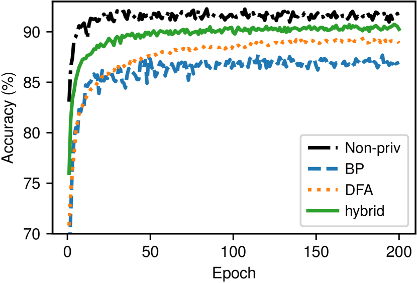
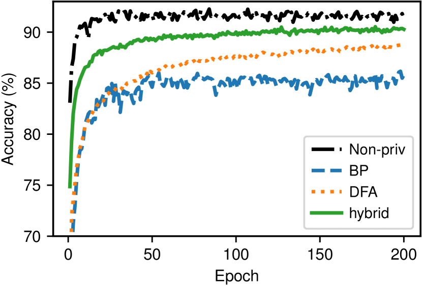
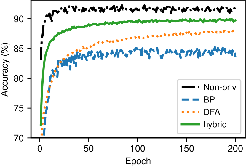
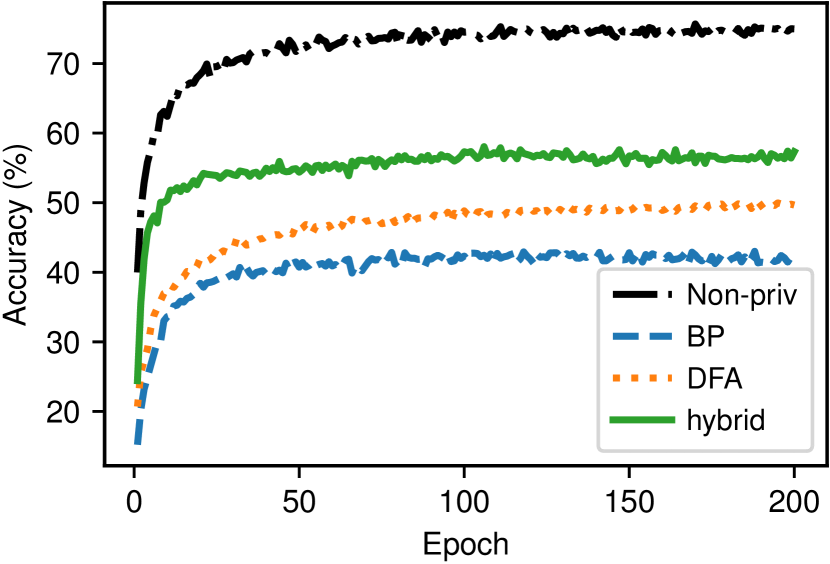
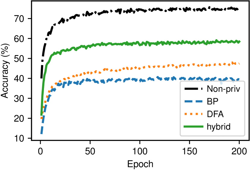
For convolutional networks, we use a similar setup to [1]. The architecture uses 2 convolutional layers (5x5 kernels and 64 channels each with 2x2 max pools) followed by 2 fully connected layers (384 units each), and the output layer uses softmax. Following [1], we set the sensitivity for each iteration at 3 (so even the DP DFA uses their setting) and a mini-batch of size 512. For DP BP, following [1], the layers use ReLU activation. ReLU is not recommended for DFA in the non-private case [26] so for DP DFA we use tanh for convolutional layers and sigmoid for fully connected layers (we use this setting even when using the differentially private DFA/BP hybrid).

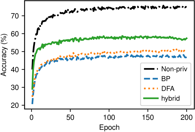
This setup ensures that each iteration and each epoch of DP BP has the same privacy impact as DP DFA. The results for Fashion MNIST are shown in Figure 2. At various noise levels $\sigma$, we see that a large gap between differentially private BP and the non-private network. Differentially private DFA outperforms DP BP, with the hybrid approach clearly outperforming both, and doing a better job of closing the gap with the non-private network. Corresponding results for CIFAR 10, which is known to be much harder for differentially private training, is shown in Figure 3. We see the same qualitative results, where the differentially private hybrid approach significantly outperforms the other privacy-preserving methods.

5.2 Fully Connected Networks.

(a) Testing accuracy, $\sigma=0.01$. At $\delta=10^{-5}$, the $\epsilon$ values at epochs 50, 100, 150, 200, 250, 300 are 9.77, 13.75, 17.8, 21.3, 23.74, and 26.19, respectively. (left: Fashon-MNIST, right CIFAR10)

(b) Testing accuracy $\sigma=0.05$. At $\delta=10^{-5}$, the $\epsilon$ values at epochs 50, 100, 150, 200, 250, 300 are 1.03, 1.46, 1.8,2.1,2.35, and 2.59, respectively. (left: Fashon-MNIST, right CIFAR10)

Figure 4: Differentially private fully connected network on Fashion-MNIST and CIFAR 10

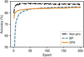
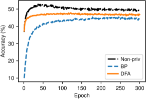
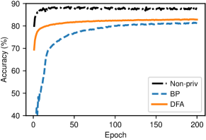
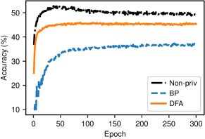
For fully connected networks, we use the following architectures. For Fashion MNIST, the network consists of two hidden layers, with 128 and 256 hidden units, respectively. These layers use the sigmoid activation function and we use softmax for the output layer. We use a minibatch of size 128 and the sensitivity of each iteration is set to 2. As usual, the privacy impact of each iteration and epoch is the same for DP BP and for DP DFA. Since CIFAR 10 is a more complex dataset, we use a more complex network with 3 hidden layers of 256 units each. The results are shown in Figure 4. We see that the accuracy of all networks saturate fairly quickly with DP DFA achieving good accuracy with fewer epochs than DP BP, suggesting that we can use it to train more accurate networks with a smaller privacy budget.

6 Conclusion

Recent advances in differential privacy have shown that privacy-preserving training of complex non-convex models is feasible. However, there is still a significant gap between accuracy of these models and application requirements. In this paper, we consider the possibility that alternatives to backprop may be more suitable for training privacy-preserving models. We proposed the first differentially private version of direct feedback alignment (DFA), a biologically inspired training algorithm.

Although the effects of DFA are not well-understood even in the non-private setting, its behavior in the privacy-preserving setting (when compared to differentially private SGD) and potential use in low-power hardware show that DFA merits increased attention and theoretical study.

References

- [1] M. Abadi, A. Chu, I. Goodfellow, H. B. McMahan, I. Mironov, K. Talwar, and L. Zhang. Deep learning with differential privacy. In Proceedings of the 2016 ACM SIGSAC Conference on Computer and Communications Security, pages 308–318. ACM, 2016.
- [2] N. C. Abay, Y. Zhou, M. Kantarcioglu, B. M. Thuraisingham, and L. Sweeney. Privacy preserving synthetic data release using deep learning. In Machine Learning and Knowledge Discovery in Databases - European Conference, ECML PKDD 2018, Dublin, Ireland, September 10-14, 2018, Proceedings, Part I, pages 510–526, 2018.
- [3] G. Acs, L. Melis, C. Castelluccia, and E. D. Cristofaro. Differentially private mixture of generative neural networks. In ICDM, 2017.
- [4] M. Akrout, C. Wilson, P. Humphreys, T. Lillicrap, and D. B. Tweed. Deep learning without weight transport. In Advances in Neural Information Processing Systems, pages 974–982, 2019.
- [5] K. Amin, A. Kulesza, A. Munoz, and S. Vassilvtiskii. Bounding user contributions: A bias-variance trade-off in differential privacy. In International Conference on Machine Learning, pages 263–271, 2019.
- [6] M. Arjovsky, S. Chintala, and L. Bottou. Wasserstein generative adversarial networks. In Proceedings of the 34th International Conference on Machine Learning, 2017.
- [7] E. Bagdasaryan, O. Poursaeed, and V. Shmatikov. Differential privacy has disparate impact on model accuracy. In Advances in Neural Information Processing Systems, pages 15453–15462, 2019.
- [8] S. Bartunov, A. Santoro, B. Richards, L. Marris, G. E. Hinton, and T. Lillicrap. Assessing the scalability of biologically-motivated deep learning algorithms and architectures. In Advances in Neural Information Processing Systems, pages 9368–9378, 2018.
- [9] B. K. Beaulieu-Jones, Z. S. Wu, C. Williams, R. Lee, S. P. Bhavnani, J. B. Byrd, and C. S. Greene. Privacy-preserving generative deep neural networks support clinical data sharing. bioRxiv, 2018.
- [10] Q. Chen, C. Xiang, M. Xue, B. Li, N. Borisov, D. Kaafar, and H. Zhu. Differentially private data generative models. https://arxiv.org/pdf/1812.02274.pdf, 2018.
- [11] B. Crafton, A. Parihar, E. Gebhardt, and A. Raychowdhury. Direct feedback alignment with sparse connections for local learning. Frontiers in Neuroscience, 13:525, 2019.
- [12] C. Dwork, K. Kenthapadi, F. McSherry, I. Mironov, and M. Naor. Our data, ourselves: Privacy via distributed noise generation. In Annual International Conference on the Theory and Applications of Cryptographic Techniques, pages 486–503. Springer, 2006.
- [13] C. Dwork, F. McSherry, K. Nissim, and A. Smith. Calibrating noise to sensitivity in private data analysis. In Theory of Cryptography Conference, pages 265–284. Springer, 2006.
- [14] I. Goodfellow, Y. Bengio, and A. Courville. Deep Learning. MIT Press, 2016. http://www.deeplearningbook.org.
- [15] S. Grossberg. Competitive learning: From interactive activation to adaptive resonance. Cognitive science, 11(1):23–63, 1987.
- [16] D. Han and H.-j. Yoo. Direct feedback alignment based convolutional neural network training for low-power online learning processor. In The IEEE International Conference on Computer Vision (ICCV) Workshops, Oct 2019.
- [17] D. Kingma and J. Ba. Adam: A method for stochastic optimization. International Conference on Learning Representations, 12 2014.
- [18] A. Krizhevsky. Learning multiple layers of features from tiny images. Technical report, 2009.
- [19] D.-H. Lee, S. Zhang, A. Fischer, and Y. Bengio. Difference target propagation. In Joint european conference on machine learning and knowledge discovery in databases, pages 498–515. Springer, 2015.
- [20] Q. Liao, J. Z. Leibo, and T. Poggio. How important is weight symmetry in backpropagation? In Thirtieth AAAI Conference on Artificial Intelligence, 2016.
- [21] T. P. Lillicrap, D. Cownden, D. B. Tweed, and C. J. Akerman. Random synaptic feedback weights support error backpropagation for deep learning. Nature communications, 7(1):1–10, 2016.
- [22] H. B. McMahan, G. Andrew, U. Erlingsson, S. Chien, I. Mironov, N. Papernot, and P. Kairouz. A general approach to adding differential privacy to iterative training procedures. arXiv preprint arXiv:1812.06210, 2018.
- [23] H. B. McMahan, D. Ramage, K. Talwar, and L. Zhang. Learning differentially private recurrent language models. In International Conference on Learning Representations, 2018.
- [24] I. Mironov. Renyi differential privacy. In Computer Security Foundations Symposium (CSF), 2017 IEEE 30th, pages 263–275. IEEE, 2017.
- [25] T. H. Moskovitz, A. Litwin-Kumar, and L. Abbott. Feedback alignment in deep convolutional networks. arXiv preprint arXiv:1812.06488, 2018.
- [26] A. Nøkland. Direct feedback alignment provides learning in deep neural networks. In Advances in neural information processing systems, pages 1037–1045, 2016.
- [27] N. Papernot, M. Abadi, Úlfar Erlingsson, I. Goodfellow, and K. Talwar. Semi-supervised knowledge transfer for deep learning from private training data. In Proceedings of the International Conference on Learning Representations, 2017.
- [28] N. Papernot, S. Song, I. Mironov, A. Raghunathan, K. Talwar, and Úlfar Erlingsson. Scalable private learning with pate. In International Conference on Learning Representations (ICLR), 2018.
- [29] N. Phan, Y. Wang, X. Wu, and D. Dou. Differential privacy preservation for deep auto-encoders: an application of human behavior prediction. In AAAI, 2016.
- [30] D. E. Rumelhart, G. E. Hinton, and R. J. Williams. Learning representations by back-propagating errors. nature, 323(6088):533–536, 1986.
- [31] R. Shokri and V. Shmatikov. Privacy-preserving deep learning. In Proceedings of the 22Nd ACM SIGSAC Conference on Computer and Communications Security, 2015.
- [32] O. Thakkar, G. Andrew, and H. B. McMahan. Differentially private learning with adaptive clipping. CoRR, abs/1905.03871, 2019.
- [33] Y.-X. Wang, B. Balle, and S. P. Kasiviswanathan. Subsampled renyi differential privacy and analytical moments accountant. In Proceedings of Machine Learning Research, volume 89, pages 1226–1235, 2019.
- [34] H. Xiao, K. Rasul, and R. Vollgraf. Fashion-mnist: a novel image dataset for benchmarking machine learning algorithms, 2017.
- [35] L. Xie, K. Lin, S. Wang, F. Wang, and J. Zhou. Differentially private generative adversarial network, 2018.
- [36] D. Xu, W. Du, and X. Wu. Removing disparate impact of differentially private stochastic gradient descent on model accuracy, 2020.
- [37] L. Yu, L. Liu, C. Pu, M. E. Gursoy, and S. Truex. Differentially private model publishing for deep learning. 2019 IEEE Symposium on Security and Privacy (SP), pages 332–349, 2019.
- [38] Y. Zhu and Y.-X. Wang. Poission subsampled rényi differential privacy. In International Conference on Machine Learning, pages 7634–7642, 2019.