The authors are supported by Grant-in-Aid for Challenging Exploratory Research (21654053).
The first author is supported by JSPS KAKENHI Grant Number 20K03601.
The second author is supported by a grant from the Simons Foundation (#708778).
1. Introduction
R. Kashaev [13 ] proposed a conjecture stating that his invariant parametrized by an integer N ≥ 2 𝑁 2 N\geq 2 [12 ] grows exponentially with growth rate proportional to the hyperbolic volume of the knot complement for any hyperbolic knot.
J. Murakami and the first author [26 ] proved that Kashaev’s invariant coincides with J N ( K ; exp ( 2 π − 1 / N ) ) subscript 𝐽 𝑁 𝐾 2 𝜋 1 𝑁
J_{N}(K;\exp(2\pi\sqrt{-1}/N))
Conjecture 1.1 (Volume Conjecture).
Let K 𝐾 K
(1.1) lim N → ∞ log | J N ( K ; exp ( 2 π − 1 / N ) ) | N = Vol ( S 3 ∖ K ) 2 π , subscript → 𝑁 subscript 𝐽 𝑁 𝐾 2 𝜋 1 𝑁
𝑁 Vol superscript 𝑆 3 𝐾 2 𝜋 \lim_{N\to\infty}\frac{\log|J_{N}(K;\exp(2\pi\sqrt{-1}/N))|}{N}=\frac{\operatorname{Vol}(S^{3}\setminus{K})}{2\pi},
where Vol Vol \operatorname{Vol} v 3 subscript 𝑣 3 v_{3} v 3 subscript 𝑣 3 v_{3}
Note that when K 𝐾 K S 3 ∖ K superscript 𝑆 3 𝐾 S^{3}\setminus{K} Vol Vol \operatorname{Vol}
It is well known that the knot complement S 3 ∖ K superscript 𝑆 3 𝐾 S^{3}\setminus{K} [8 , 9 ] ) and that Vol ( S 3 ∖ K ) Vol superscript 𝑆 3 𝐾 \operatorname{Vol}(S^{3}\setminus{K}) Vol ( S 3 ∖ K ) = 0 Vol superscript 𝑆 3 𝐾 0 \operatorname{Vol}(S^{3}\setminus{K})=0 [14 ] proved that when K 𝐾 K 1.1
For hyperbolic knots, T. Ekholm showed that the volume conjecture is true for the figure-eight knot 4 1 subscript 4 1 4_{1} 5 2 subscript 5 2 5_{2} [29 ] , and for 6 1 , 6 2 , 6 3 subscript 6 1 subscript 6 2 subscript 6 3
6_{1},6_{2},6_{3} [30 ] .
For non-hyperbolic knots with non-zero volumes, H. Zheng [33 ] proved the volume conjecture in the case of Whitehead doubles of the torus knot of type ( 2 , 2 b + 1 ) 2 2 𝑏 1 (2,2b+1) [18 ] .
What happens when we replace 2 π − 1 2 𝜋 1 2\pi\sqrt{-1} J N ( K ; e 2 π − 1 / N ) subscript 𝐽 𝑁 𝐾 superscript 𝑒 2 𝜋 1 𝑁
J_{N}\left(K;e^{2\pi\sqrt{-1}/N}\right) η 𝜂 \eta
In the case of the figure-eight knot E 𝐸 E J N ( E ; e η / N ) subscript 𝐽 𝑁 𝐸 superscript 𝑒 𝜂 𝑁
J_{N}\left(E;e^{\eta/N}\right) N → ∞ → 𝑁 N\to\infty
(i)
| 2 π − 1 − η | 2 𝜋 1 𝜂 |2\pi\sqrt{-1}-\eta| η 𝜂 \eta
lim N → ∞ log J N ( E ; e η / N ) N subscript → 𝑁 subscript 𝐽 𝑁 𝐸 superscript 𝑒 𝜂 𝑁
𝑁 \lim_{N\to\infty}\frac{\log J_{N}(E;e^{\eta/N})}{N}
exists and it determines the volume and the Chern–Simons invariant of the three-manifold obtained by generalized Dehn surgery corresponding to η − 2 π − 1 𝜂 2 𝜋 1 \eta-2\pi\sqrt{-1} [27 ] (see also [24 ] ).
(ii)
η 𝜂 \eta 2 π / | η | 2 𝜋 𝜂 2\pi/|\eta| 5 π / 3 < | η | < 7 π / 3 5 𝜋 3 𝜂 7 𝜋 3 5\pi/3<|\eta|<7\pi/3
lim N → ∞ log | J N ( E ; e η / N ) | N = Vol ( E | η − 2 π − 1 | ) η , subscript → 𝑁 subscript 𝐽 𝑁 𝐸 superscript 𝑒 𝜂 𝑁
𝑁 Vol subscript 𝐸 𝜂 2 𝜋 1 𝜂 \lim_{N\to\infty}\frac{\log\left|J_{N}\left(E;e^{\eta/N}\right)\right|}{N}=\frac{\operatorname{Vol}\left(E_{|\eta-2\pi\sqrt{-1}|}\right)}{\eta},
where E θ subscript 𝐸 𝜃 E_{\theta} E 𝐸 E θ 𝜃 \theta [21 , Theorem 1.2] (see [25 ] for a correction).
(iii)
η 𝜂 \eta η > 2 κ 𝜂 2 𝜅 \eta>2\kappa κ := arccosh ( 3 / 2 ) / 2 = log ( ( 3 + 5 ) / 2 ) / 2 assign 𝜅 arccosh 3 2 2 3 5 2 2 \kappa:=\operatorname{arccosh}(3/2)/2=\log\bigl{(}(3+\sqrt{5})/2\bigr{)}/2
(1.2) lim N → ∞ log | J N ( E ; e η / N ) | N = 1 η S ( η / 2 ) , subscript → 𝑁 subscript 𝐽 𝑁 𝐸 superscript 𝑒 𝜂 𝑁
𝑁 1 𝜂 𝑆 𝜂 2 \lim_{N\to\infty}\frac{\log\left|J_{N}\left(E;e^{\eta/N}\right)\right|}{N}=\frac{1}{\eta}S(\eta/2),
where
S ( ξ ) := Li 2 ( e − φ ( ξ ) − 2 ξ ) − Li 2 ( e φ ( ξ ) − 2 ξ ) + 2 ξ φ ( ξ ) assign 𝑆 𝜉 subscript Li 2 superscript 𝑒 𝜑 𝜉 2 𝜉 subscript Li 2 superscript 𝑒 𝜑 𝜉 2 𝜉 2 𝜉 𝜑 𝜉 S(\xi):=\operatorname{Li}_{2}\left(e^{-\varphi(\xi)-2\xi}\right)-\operatorname{Li}_{2}\left(e^{\varphi(\xi)-2\xi}\right)+2\xi\varphi(\xi)
with φ ( ξ ) := arccosh ( cosh ( 2 ξ ) − 1 / 2 ) assign 𝜑 𝜉 arccosh 2 𝜉 1 2 \varphi(\xi):=\operatorname{arccosh}(\cosh(2\xi)-1/2) Li 2 ( z ) := − ∫ 0 z log ( 1 − x ) x 𝑑 x assign subscript Li 2 𝑧 superscript subscript 0 𝑧 1 𝑥 𝑥 differential-d 𝑥 \operatorname{Li}_{2}(z):=-\int_{0}^{z}\frac{\log(1-x)}{x}\,dx [21 , Theorem 8.1] and [23 , Theorem 6.9] .
(iv)
η = 2 κ 𝜂 2 𝜅 \eta=2\kappa J N ( E ; e η / N ) subscript 𝐽 𝑁 𝐸 superscript 𝑒 𝜂 𝑁
J_{N}\left(E;e^{\eta/N}\right) N 𝑁 N
J N ( E ; e 2 κ / N ) ∼ N → ∞ Γ ( 1 / 3 ) ( 6 κ ) 2 / 3 N 2 / 3 , subscript 𝐽 𝑁 𝐸 superscript 𝑒 2 𝜅 𝑁
→ 𝑁 similar-to Γ 1 3 superscript 6 𝜅 2 3 superscript 𝑁 2 3 J_{N}\left(E;e^{2\kappa/N}\right)\underset{N\to\infty}{\sim}\frac{\Gamma(1/3)}{(6\kappa)^{2/3}}N^{2/3},
where Γ ( x ) Γ 𝑥 \Gamma(x) f ( N ) ∼ N → ∞ g ( N ) 𝑓 𝑁 → 𝑁 similar-to 𝑔 𝑁 f(N)\underset{N\to\infty}{\sim}g(N) lim N → ∞ f ( N ) g ( N ) = 1 subscript → 𝑁 𝑓 𝑁 𝑔 𝑁 1 \lim_{N\to\infty}\frac{f(N)}{g(N)}=1 [7 , Theorem 1.1] ).
(v)
| η | 𝜂 |\eta| lim N → ∞ log | J N ( E ; e η / N ) | N = 0 subscript → 𝑁 subscript 𝐽 𝑁 𝐸 superscript 𝑒 𝜂 𝑁
𝑁 0 \lim_{N\to\infty}\frac{\log\left|J_{N}\left(E;e^{\eta/N}\right)\right|}{N}=0
lim N → ∞ J N ( E ; e η / N ) = 1 Δ ( E ; e η ) , subscript → 𝑁 subscript 𝐽 𝑁 𝐸 superscript 𝑒 𝜂 𝑁
1 Δ 𝐸 superscript 𝑒 𝜂
\lim_{N\to\infty}J_{N}\left(E;e^{\eta/N}\right)=\frac{1}{\Delta(E;e^{\eta})},
where Δ ( K ; t ) Δ 𝐾 𝑡
\Delta(K;t) K 𝐾 K Δ ( K ; 1 ) = 1 Δ 𝐾 1
1 \Delta(K;1)=1 Δ ( K ; t − 1 ) = Δ ( K ; t ) Δ 𝐾 superscript 𝑡 1
Δ 𝐾 𝑡
\Delta(K;t^{-1})=\Delta(K;t) [22 ] ).
This is also true for any knot [4 , Theorem 1.3] .
See [5 , 2 , 3 ] for more results.
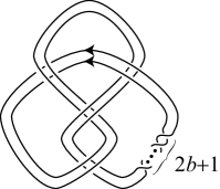
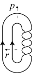
In this paper, we study the colored Jones polynomial of the ( 2 , 2 b + 1 ) 2 2 𝑏 1 (2,2b+1) 1 E ( 2 , 2 b + 1 ) superscript 𝐸 2 2 𝑏 1 E^{(2,2b+1)}
Figure 1. ( 2 , 2 b + 1 ) 2 2 𝑏 1 (2,2b+1) E ( 2 , 2 b + 1 ) superscript 𝐸 2 2 𝑏 1 E^{(2,2b+1)}
We put κ := arccosh ( 3 / 2 ) / 2 assign 𝜅 arccosh 3 2 2 \kappa:=\operatorname{arccosh}(3/2)/2 ℱ := S 3 ∖ Int N ( E ( 2 , 2 b + 1 ) ) assign ℱ superscript 𝑆 3 Int 𝑁 superscript 𝐸 2 2 𝑏 1 \mathcal{F}:=S^{3}\setminus\operatorname{Int}{N(E^{(2,2b+1)})} N ( E ( 2 , 2 b + 1 ) ) 𝑁 superscript 𝐸 2 2 𝑏 1 N(E^{(2,2b+1)}) E ( 2 , 2 b + 1 ) superscript 𝐸 2 2 𝑏 1 E^{(2,2b+1)} S 3 superscript 𝑆 3 S^{3} Int Int \operatorname{Int}
Theorem (Theorem 5.3 .
Let ξ 𝜉 \xi ξ > κ 𝜉 𝜅 \xi>\kappa
ξ lim N → ∞ log J N ( E ( 2 , 2 b + 1 ) ; e ξ / N ) N = S ( ξ ) , 𝜉 subscript → 𝑁 subscript 𝐽 𝑁 superscript 𝐸 2 2 𝑏 1 superscript 𝑒 𝜉 𝑁
𝑁 𝑆 𝜉 \xi\lim_{N\to\infty}\frac{\log J_{N}\left(E^{(2,2b+1)};e^{\xi/N}\right)}{N}=S(\xi),
where we put
S ( ξ ) := Li 2 ( e − φ ( ξ ) − 2 ξ ) − Li 2 ( e φ ( ξ ) − 2 ξ ) + 2 ξ φ ( ξ ) assign 𝑆 𝜉 subscript Li 2 superscript 𝑒 𝜑 𝜉 2 𝜉 subscript Li 2 superscript 𝑒 𝜑 𝜉 2 𝜉 2 𝜉 𝜑 𝜉 S(\xi):=\operatorname{Li}_{2}\left(e^{-\varphi(\xi)-2\xi}\right)-\operatorname{Li}_{2}\left(e^{\varphi(\xi)-2\xi}\right)+2\xi\varphi(\xi)
with
φ ( ξ ) := arccosh ( cosh ( 2 ξ ) − 1 2 ) . assign 𝜑 𝜉 arccosh 2 𝜉 1 2 \varphi(\xi):=\operatorname{arccosh}\left(\cosh(2\xi)-\frac{1}{2}\right).
Moreover, S ( ξ ) 𝑆 𝜉 S(\xi) CS ℱ ( [ ρ ξ ] ; ξ , v ( ξ ) ) subscript CS ℱ delimited-[] subscript 𝜌 𝜉 𝜉 𝑣 𝜉 \operatorname{CS}_{\mathcal{F}}([\rho_{\xi}];\xi,v(\xi)) ℱ ℱ \mathcal{F} ρ ξ : π 1 ( ℱ ) → SL ( 2 ; ℂ ) : subscript 𝜌 𝜉 → subscript 𝜋 1 ℱ SL 2 ℂ
\rho_{\xi}\colon\pi_{1}(\mathcal{F})\to\mathrm{SL}(2;\mathbb{C}) ( ξ , v ( ξ ) ) 𝜉 𝑣 𝜉 (\xi,v(\xi)) (see Section 5 ) in the following way:
CS ℱ ( [ ρ ξ ] ; ξ , v ( ξ ) ) = S ( ξ ) − ξ v ( ξ ) 4 . subscript CS ℱ delimited-[] subscript 𝜌 𝜉 𝜉 𝑣 𝜉 𝑆 𝜉 𝜉 𝑣 𝜉 4 \operatorname{CS}_{\mathcal{F}}([\rho_{\xi}];\xi,v(\xi))=S(\xi)-\frac{\xi v(\xi)}{4}.
Here ρ ξ subscript 𝜌 𝜉 \rho_{\xi} ∂ ℱ ℱ \partial\mathcal{F} ( e ξ / 2 0 0 e − ξ / 2 ) matrix superscript 𝑒 𝜉 2 0 0 superscript 𝑒 𝜉 2 \begin{pmatrix}e^{\xi/2}&0\\
0&e^{-\xi/2}\end{pmatrix} ( e v ( ξ ) / 2 0 0 e − v ( ξ ) / 2 ) matrix superscript 𝑒 𝑣 𝜉 2 0 0 superscript 𝑒 𝑣 𝜉 2 \begin{pmatrix}e^{v(\xi)/2}&0\\
0&e^{-v(\xi)/2}\end{pmatrix}
Compare this with the following, which was proved in [21 , Theorem 8.1] and [23 , Theorem 6.9] (see (1.2 ℰ = S 3 ∖ Int N ( E ) ℰ superscript 𝑆 3 Int 𝑁 𝐸 \mathcal{E}=S^{3}\setminus\operatorname{Int}{N(E)}
Theorem (Theorem 5.4 .
Let η 𝜂 \eta η > 2 κ 𝜂 2 𝜅 \eta>2\kappa
η lim N → ∞ J N ( E ; e η / N ) N = S ( η / 2 ) . 𝜂 subscript → 𝑁 subscript 𝐽 𝑁 𝐸 superscript 𝑒 𝜂 𝑁
𝑁 𝑆 𝜂 2 \eta\lim_{N\to\infty}\frac{J_{N}(E;e^{\eta/N})}{N}=S(\eta/2).
Moreover we have
CS ℰ ( [ σ η ] ; η , v E ( η ) ) = S ( η / 2 ) − η v E ( η ) 4 , subscript CS ℰ delimited-[] subscript 𝜎 𝜂 𝜂 subscript 𝑣 𝐸 𝜂 𝑆 𝜂 2 𝜂 subscript 𝑣 𝐸 𝜂 4 \operatorname{CS}_{\mathcal{E}}([\sigma_{\eta}];\eta,v_{E}(\eta))=S(\eta/2)-\frac{\eta v_{E}(\eta)}{4},
where σ η subscript 𝜎 𝜂 \sigma_{\eta} ∂ ℰ ℰ \partial\mathcal{E} ( e η / 2 0 0 e − η / 2 ) matrix superscript 𝑒 𝜂 2 0 0 superscript 𝑒 𝜂 2 \begin{pmatrix}e^{\eta/2}&0\\
0&e^{-\eta/2}\end{pmatrix} ( e v E ( η ) / 2 0 0 e − v E ( η ) / 2 ) matrix superscript 𝑒 subscript 𝑣 𝐸 𝜂 2 0 0 superscript 𝑒 subscript 𝑣 𝐸 𝜂 2 \begin{pmatrix}e^{v_{E}(\eta)/2}&0\\
0&e^{-v_{E}(\eta)/2}\end{pmatrix}
2. Preliminaries
In this section, we use linear skein theory (see for example [19 , Chapters 13, 14] ) to calculate the colored Jones polynomial.
For another way to calculate it, see [18 ] .
The N 𝑁 N E ( 2 , 2 b + 1 ) superscript 𝐸 2 2 𝑏 1 E^{(2,2b+1)}
1 Δ N − 1 ( ( − 1 ) N − 1 A ( N − 1 ) 2 + 2 ( N − 1 ) ) − ( 2 b + 1 ) ⟨ ⟩ | A := t 1 / 4 , evaluated-at 1 subscript Δ 𝑁 1 superscript superscript 1 𝑁 1 superscript 𝐴 superscript 𝑁 1 2 2 𝑁 1 2 𝑏 1 delimited-⟨⟩ assign 𝐴 superscript 𝑡 1 4 \left.\frac{1}{\Delta_{N-1}}\left((-1)^{N-1}A^{(N-1)^{2}+2(N-1)}\right)^{-(2b+1)}\left\langle\raisebox{-0.5pt}{\includegraphics[scale={0.2}]{E2_2b+1.eps}}\right\rangle\right|_{A:=t^{1/4}},
where the number N − 1 𝑁 1 N-1 ( N − 1 ) 𝑁 1 (N-1) [10 , 32 ] along the line, ⟨ D ⟩ delimited-⟨⟩ 𝐷 \langle D\rangle [15 ] of a link diagram D 𝐷 D Δ k := ( − 1 ) k A 2 ( k + 1 ) − A − 2 ( k + 1 ) A 2 − A − 2 assign subscript Δ 𝑘 superscript 1 𝑘 superscript 𝐴 2 𝑘 1 superscript 𝐴 2 𝑘 1 superscript 𝐴 2 superscript 𝐴 2 \Delta_{k}:=(-1)^{k}\frac{A^{2(k+1)-A^{-2(k+1)}}}{A^{2}-A^{-2}} ( 2 b + 1 ) 2 𝑏 1 (2b+1) ( ( − 1 ) N − 1 A ( N − 1 ) 2 + 2 ( N − 1 ) ) − ( 2 b + 1 ) superscript superscript 1 𝑁 1 superscript 𝐴 superscript 𝑁 1 2 2 𝑁 1 2 𝑏 1 \left((-1)^{N-1}A^{(N-1)^{2}+2(N-1)}\right)^{-(2b+1)} [19 , Lemma 14.1] ).
We use the notation described in [19 , Chapters 13, 14] .
By using identities in [19 , Chapter 14] , we have
(2.1) ⟨ ⟩ = (Figure 14.15 in [19 ] ) ∑ c : even , 0 ≤ c ≤ 2 ( N − 1 ) Δ c θ ( N − 1 , N − 1 , c ) ⟨ ⟩ = (Figure 14.14 in [19 ] ) ∑ c ( − 1 ) N − 1 − c / 2 A ( 2 b + 1 ) ( − 2 N + 2 + c − ( N − 1 ) 2 + c 2 / 2 ) Δ c θ ( N − 1 , N − 1 , c ) ⟨ ⟩ = (Reidemeister moves II and III) ∑ c ( − 1 ) N − 1 − c / 2 A ( 2 b + 1 ) ( − N 2 + 1 + c + c 2 / 2 ) Δ c θ ( N − 1 , N − 1 , c ) ⟨ ⟩ = (Figure 14.8 in [19 ] ) ∑ c ( − 1 ) N − 1 − c / 2 A ( 2 b + 1 ) ( − N 2 + 1 + c + c 2 / 2 ) ⟨ ⟩ . delimited-⟨⟩ (Figure 14.15 in [19 ] ) subscript : 𝑐 even 0
𝑐 2 𝑁 1 subscript Δ 𝑐 𝜃 𝑁 1 𝑁 1 𝑐 delimited-⟨⟩ (Figure 14.14 in [19 ] ) subscript 𝑐 superscript 1 𝑁 1 𝑐 2 superscript 𝐴 2 𝑏 1 2 𝑁 2 𝑐 superscript 𝑁 1 2 superscript 𝑐 2 2 subscript Δ 𝑐 𝜃 𝑁 1 𝑁 1 𝑐 delimited-⟨⟩ (Reidemeister moves II and III) subscript 𝑐 superscript 1 𝑁 1 𝑐 2 superscript 𝐴 2 𝑏 1 superscript 𝑁 2 1 𝑐 superscript 𝑐 2 2 subscript Δ 𝑐 𝜃 𝑁 1 𝑁 1 𝑐 delimited-⟨⟩ (Figure 14.8 in [19 ] ) subscript 𝑐 superscript 1 𝑁 1 𝑐 2 superscript 𝐴 2 𝑏 1 superscript 𝑁 2 1 𝑐 superscript 𝑐 2 2 delimited-⟨⟩ \begin{split}&\left\langle\raisebox{-0.5pt}{\includegraphics[scale={0.3}]{E2_2b+1.eps}}\right\rangle\\
=&\\
&\text{(Figure~{}14.15 in \cite[cite]{[\@@bibref{}{Lickorish:1997}{}{}]})}\\
&\sum_{c\colon\text{even},0\leq c\leq 2(N-1)}\frac{\Delta_{c}}{\theta(N-1,N-1,c)}\left\langle\raisebox{-0.5pt}{\includegraphics[scale={0.3}]{E2_c_2b+1.eps}}\right\rangle\\
=&\\
&\text{(Figure~{}14.14 in \cite[cite]{[\@@bibref{}{Lickorish:1997}{}{}]})}\\
&\sum_{c}(-1)^{N-1-c/2}A^{(2b+1)(-2N+2+c-(N-1)^{2}+c^{2}/2)}\frac{\Delta_{c}}{\theta(N-1,N-1,c)}\left\langle\raisebox{-0.5pt}{\includegraphics[scale={0.3}]{E2_d.eps}}\right\rangle\\
=&\\
&\text{(Reidemeister moves II and III)}\\
&\sum_{c}(-1)^{N-1-c/2}A^{(2b+1)(-N^{2}+1+c+c^{2}/2)}\frac{\Delta_{c}}{\theta(N-1,N-1,c)}\left\langle\raisebox{-0.5pt}{\includegraphics[scale={0.3}]{E_c_N-1_N-1.eps}}\right\rangle\\
=&\\
&\text{(Figure~{}14.8 in \cite[cite]{[\@@bibref{}{Lickorish:1997}{}{}]})}\\
&\sum_{c}(-1)^{N-1-c/2}A^{(2b+1)(-N^{2}+1+c+c^{2}/2)}\left\langle\raisebox{-0.5pt}{\includegraphics[scale={0.3}]{E_2.eps}}\right\rangle.\end{split}
Now ⟨ ⟩ delimited-⟨⟩ \left\langle\raisebox{-0.5pt}{\includegraphics[scale={0.3}]{E_2.eps}}\right\rangle ( J c + 1 ( E ; t ) | t := A 4 ) Δ c + 1 \left(J_{c+1}(E;t)\Bigm{|}_{t:=A^{4}}\right)\Delta_{c+1}
Proposition 2.1 .
We have
J N ( E ( 2 , 2 b + 1 ) ; t ) = ( − 1 ) N − 1 t − ( 2 b + 1 ) ( N 2 − 1 ) / 2 t N / 2 − t − N / 2 ∑ d = 0 N − 1 ( − 1 ) d t ( 2 b + 1 ) ( d 2 + d ) / 2 ( t ( 2 d + 1 ) / 2 − t − ( 2 d + 1 ) / 2 ) × ∑ l = 0 2 d ∏ k = 1 l ( t ( 2 d + 1 + k ) / 2 − t − ( 2 d + 1 + k ) / 2 ) ( t ( 2 d + 1 − k ) / 2 − t − ( 2 d + 1 − k ) / 2 ) . subscript 𝐽 𝑁 superscript 𝐸 2 2 𝑏 1 𝑡
superscript 1 𝑁 1 superscript 𝑡 2 𝑏 1 superscript 𝑁 2 1 2 superscript 𝑡 𝑁 2 superscript 𝑡 𝑁 2 superscript subscript 𝑑 0 𝑁 1 superscript 1 𝑑 superscript 𝑡 2 𝑏 1 superscript 𝑑 2 𝑑 2 superscript 𝑡 2 𝑑 1 2 superscript 𝑡 2 𝑑 1 2 superscript subscript 𝑙 0 2 𝑑 superscript subscript product 𝑘 1 𝑙 superscript 𝑡 2 𝑑 1 𝑘 2 superscript 𝑡 2 𝑑 1 𝑘 2 superscript 𝑡 2 𝑑 1 𝑘 2 superscript 𝑡 2 𝑑 1 𝑘 2 \begin{split}&J_{N}\left(E^{(2,2b+1)};t\right)\\
=&\frac{(-1)^{N-1}t^{-(2b+1)(N^{2}-1)/2}}{t^{N/2}-t^{-N/2}}\sum_{d=0}^{N-1}(-1)^{d}t^{(2b+1)(d^{2}+d)/2}\left(t^{(2d+1)/2}-t^{-(2d+1)/2}\right)\\
&\times\sum_{l=0}^{2d}\prod_{k=1}^{l}\left(t^{(2d+1+k)/2}-t^{-(2d+1+k)/2}\right)\left(t^{(2d+1-k)/2}-t^{-(2d+1-k)/2}\right).\end{split}
Proof.
From (2.1
( − 1 ) N − 1 t N / 2 − t − N / 2 t 1 / 2 − t − 1 / 2 J N ( E ( 2 , 2 b + 1 ) ; t ) = ( ( − 1 ) N − 1 A ( N − 1 ) 2 + 2 ( N − 1 ) ) − ( 2 b + 1 ) × ∑ 0 ≤ c ≤ 2 ( N − 1 ) c : even ( − 1 ) N − 1 − c / 2 A ( 2 b + 1 ) ( − N 2 + 1 + c + c 2 / 2 ) ( J c + 1 ( E ; t ) | t := A 4 ) Δ c + 1 | A := t 1 / 4 = ( c := 2 d ) ∑ d = 0 N − 1 t ( 2 d + 1 ) / 2 − t − ( 2 d + 1 ) / 2 t 1 / 2 − t − 1 / 2 ( − 1 ) N − 1 − d t ( 2 b + 1 ) ( − N 2 + 1 + 2 d + 2 d 2 ) / 4 J c + 1 ( E ; t ) = ( − 1 ) N − 1 t − ( 2 b + 1 ) ( N 2 − 1 ) / 2 t 1 / 2 − t − 1 / 2 ∑ d = 0 N − 1 ( t ( 2 d + 1 ) / 2 − t − ( 2 d + 1 ) / 2 ) ( − 1 ) d t ( 2 b + 1 ) ( d + d 2 ) / 2 J 2 d + 1 ( E ; t ) . \begin{split}&(-1)^{N-1}\frac{t^{N/2}-t^{-N/2}}{t^{1/2}-t^{-1/2}}J_{N}\left(E^{(2,2b+1)};t\right)\\
=&((-1)^{N-1}A^{(N-1)^{2}+2(N-1)})^{-(2b+1)}\\
&\times\left.\sum_{\begin{subarray}{c}0\leq c\leq 2(N-1)\\
\text{$c$: even}\end{subarray}}(-1)^{N-1-c/2}A^{(2b+1)(-N^{2}+1+c+c^{2}/2)}\left(J_{c+1}(E;t)\Bigm{|}_{t:=A^{4}}\right)\Delta_{c+1}\right|_{A:=t^{1/4}}\\
=&\\
&\text{($c:=2d$)}\\
&\sum_{d=0}^{N-1}\frac{t^{(2d+1)/2}-t^{-(2d+1)/2}}{t^{1/2}-t^{-1/2}}(-1)^{N-1-d}t^{(2b+1)(-N^{2}+1+2d+2d^{2})/4}J_{c+1}(E;t)\\
=&(-1)^{N-1}\frac{t^{-(2b+1)(N^{2}-1)/2}}{t^{1/2}-t^{-1/2}}\sum_{d=0}^{N-1}\left(t^{(2d+1)/2}-t^{-(2d+1)/2}\right)(-1)^{d}t^{(2b+1)(d+d^{2})/2}J_{2d+1}(E;t).\end{split}
Now using the following formula of the m 𝑚 m [6 , 20 ]
J m ( E ; t ) = ∑ l = 0 m − 1 ∏ k = 1 l ( t ( m + k ) / 2 − t − ( m + k ) / 2 ) ( t ( m − k ) / 2 − t − ( m − k ) / 2 ) , subscript 𝐽 𝑚 𝐸 𝑡
superscript subscript 𝑙 0 𝑚 1 superscript subscript product 𝑘 1 𝑙 superscript 𝑡 𝑚 𝑘 2 superscript 𝑡 𝑚 𝑘 2 superscript 𝑡 𝑚 𝑘 2 superscript 𝑡 𝑚 𝑘 2 J_{m}(E;t)=\sum_{l=0}^{m-1}\prod_{k=1}^{l}\left(t^{(m+k)/2}-t^{-(m+k)/2}\right)\left(t^{(m-k)/2}-t^{-(m-k)/2}\right),
we obtain the required formula.
∎
3. Limit
Fix a positive real number ξ 𝜉 \xi 2.1
J N ( E ( 2 , 2 b + 1 ) ; e ξ / N ) = ( − 1 ) N − 1 exp ( − ( 2 b + 1 ) ( N 2 − 1 ) ξ 2 N ) 2 sinh ( ξ / 2 ) ∑ d = 0 N − 1 ∑ l = 0 2 d ( − 1 ) d f d , l subscript 𝐽 𝑁 superscript 𝐸 2 2 𝑏 1 superscript 𝑒 𝜉 𝑁
superscript 1 𝑁 1 2 𝑏 1 superscript 𝑁 2 1 𝜉 2 𝑁 2 𝜉 2 superscript subscript 𝑑 0 𝑁 1 superscript subscript 𝑙 0 2 𝑑 superscript 1 𝑑 subscript 𝑓 𝑑 𝑙
J_{N}\left(E^{(2,2b+1)};e^{\xi/N}\right)=\frac{(-1)^{N-1}\exp\left(-\frac{(2b+1)(N^{2}-1)\xi}{2N}\right)}{2\sinh(\xi/2)}\sum_{d=0}^{N-1}\sum_{l=0}^{2d}(-1)^{d}f_{d,l}
with
f d , l = exp ( ( 2 b + 1 ) ( d 2 + d ) ξ 2 N ) × 2 sinh ( ( 2 d + 1 ) ξ 2 N ) × ∏ k = 1 l 4 sinh ( ( 2 d + 1 + k ) ξ 2 N ) sinh ( ( 2 d + 1 − k ) ξ 2 N ) . subscript 𝑓 𝑑 𝑙
2 𝑏 1 superscript 𝑑 2 𝑑 𝜉 2 𝑁 2 2 𝑑 1 𝜉 2 𝑁 superscript subscript product 𝑘 1 𝑙 4 2 𝑑 1 𝑘 𝜉 2 𝑁 2 𝑑 1 𝑘 𝜉 2 𝑁 f_{d,l}=\exp\left(\frac{(2b+1)(d^{2}+d)\xi}{2N}\right)\times 2\sinh\left(\frac{(2d+1)\xi}{2N}\right)\\
\times\prod_{k=1}^{l}4\sinh\left(\frac{(2d+1+k)\xi}{2N}\right)\sinh\left(\frac{(2d+1-k)\xi}{2N}\right).
Lemma 3.1 .
Let l 𝑙 l d 𝑑 d 1 ≤ d ≤ N − 1 1 𝑑 𝑁 1 1\leq d\leq N-1 0 ≤ l ≤ 2 d − 2 0 𝑙 2 𝑑 2 0\leq l\leq 2d-2 f d , l > f d − 1 , l subscript 𝑓 𝑑 𝑙
subscript 𝑓 𝑑 1 𝑙
f_{d,l}>f_{d-1,l}
Proof.
We first note that f d , l subscript 𝑓 𝑑 𝑙
f_{d,l}
(3.1) f d , l f d − 1 , l = exp ( ( 2 b + 1 ) d ξ N ) sinh ( ( 2 d + 1 ) ξ 2 N ) sinh ( ( 2 d − 1 ) ξ 2 N ) ∏ k = 1 l sinh ( ( 2 d + 1 + k ) ξ 2 N ) sinh ( ( 2 d − 1 + k ) ξ 2 N ) sinh ( ( 2 d + 1 − k ) ξ 2 N ) sinh ( ( 2 d − 1 − k ) ξ 2 N ) . subscript 𝑓 𝑑 𝑙
subscript 𝑓 𝑑 1 𝑙
2 𝑏 1 𝑑 𝜉 𝑁 2 𝑑 1 𝜉 2 𝑁 2 𝑑 1 𝜉 2 𝑁 superscript subscript product 𝑘 1 𝑙 2 𝑑 1 𝑘 𝜉 2 𝑁 2 𝑑 1 𝑘 𝜉 2 𝑁 2 𝑑 1 𝑘 𝜉 2 𝑁 2 𝑑 1 𝑘 𝜉 2 𝑁 \frac{f_{d,l}}{f_{d-1,l}}=\exp\left(\frac{(2b+1)d\xi}{N}\right)\frac{\sinh\left(\frac{(2d+1)\xi}{2N}\right)}{\sinh\left(\frac{(2d-1)\xi}{2N}\right)}\prod_{k=1}^{l}\frac{\sinh\left(\frac{(2d+1+k)\xi}{2N}\right)}{\sinh\left(\frac{(2d-1+k)\xi}{2N}\right)}\frac{\sinh\left(\frac{(2d+1-k)\xi}{2N}\right)}{\sinh\left(\frac{(2d-1-k)\xi}{2N}\right)}.
Since ξ > 0 𝜉 0 \xi>0
exp ( ( 2 b + 1 ) d ξ N ) 2 𝑏 1 𝑑 𝜉 𝑁 \displaystyle\exp\left(\frac{(2b+1)d\xi}{N}\right) > 1 , absent 1 \displaystyle>1,
sinh ( ( 2 d + 1 ) ξ 2 N ) sinh ( ( 2 d − 1 ) ξ 2 N ) 2 𝑑 1 𝜉 2 𝑁 2 𝑑 1 𝜉 2 𝑁 \displaystyle\frac{\sinh\left(\frac{(2d+1)\xi}{2N}\right)}{\sinh\left(\frac{(2d-1)\xi}{2N}\right)} > 1 , absent 1 \displaystyle>1,
sinh ( ( 2 d + 1 + k ) ξ 2 N ) sinh ( ( 2 d − 1 + k ) ξ 2 N ) 2 𝑑 1 𝑘 𝜉 2 𝑁 2 𝑑 1 𝑘 𝜉 2 𝑁 \displaystyle\frac{\sinh\left(\frac{(2d+1+k)\xi}{2N}\right)}{\sinh\left(\frac{(2d-1+k)\xi}{2N}\right)} > 1 , absent 1 \displaystyle>1,
sinh ( ( 2 d + 1 − k ) ξ 2 N ) sinh ( ( 2 d − 1 − k ) ξ 2 N ) 2 𝑑 1 𝑘 𝜉 2 𝑁 2 𝑑 1 𝑘 𝜉 2 𝑁 \displaystyle\frac{\sinh\left(\frac{(2d+1-k)\xi}{2N}\right)}{\sinh\left(\frac{(2d-1-k)\xi}{2N}\right)} > 1 . absent 1 \displaystyle>1.
Therefore we have the required inequality.
∎
Corollary 3.2 .
For any l 𝑙 l d 𝑑 d 0 ≤ d ≤ N − 2 0 𝑑 𝑁 2 0\leq d\leq N-2 0 ≤ l ≤ 2 d 0 𝑙 2 𝑑 0\leq l\leq 2d
f d , l < f N − 1 , l . subscript 𝑓 𝑑 𝑙
subscript 𝑓 𝑁 1 𝑙
f_{d,l}<f_{N-1,l}.
Define
S := ( − 1 ) N − 1 ∑ d = 0 N − 1 ∑ l = 0 2 d ( − 1 ) d f d , l assign 𝑆 superscript 1 𝑁 1 superscript subscript 𝑑 0 𝑁 1 superscript subscript 𝑙 0 2 𝑑 superscript 1 𝑑 subscript 𝑓 𝑑 𝑙
S:=(-1)^{N-1}\sum_{d=0}^{N-1}\sum_{l=0}^{2d}(-1)^{d}f_{d,l}
so that
J N ( E ( 2 , 2 b + 1 ) ; e ξ / N ) = exp ( − ( 2 b + 1 ) ( N 2 − 1 ) ξ 2 N ) 2 sinh ( ξ / 2 ) S . subscript 𝐽 𝑁 superscript 𝐸 2 2 𝑏 1 superscript 𝑒 𝜉 𝑁
2 𝑏 1 superscript 𝑁 2 1 𝜉 2 𝑁 2 𝜉 2 𝑆 J_{N}\left(E^{(2,2b+1)};e^{\xi/N}\right)=\frac{\exp\left(-\frac{(2b+1)(N^{2}-1)\xi}{2N}\right)}{2\sinh(\xi/2)}S.
Then we have the following lemma.
Lemma 3.3 .
The following inequality holds.
S > ( 1 − e − ξ / 2 ) ∑ l = 0 2 N − 2 f N − 1 , l . 𝑆 1 superscript 𝑒 𝜉 2 superscript subscript 𝑙 0 2 𝑁 2 subscript 𝑓 𝑁 1 𝑙
S>(1-e^{-\xi/2})\sum_{l=0}^{2N-2}f_{N-1,l}.
Proof.
From (3.1
(3.2) f N − 1 , l f N − 2 , l > e ( 2 b + 1 ) ( N − 1 ) ξ / N ≥ e ( N − 1 ) ξ / N ≥ e ξ / 2 subscript 𝑓 𝑁 1 𝑙
subscript 𝑓 𝑁 2 𝑙
superscript 𝑒 2 𝑏 1 𝑁 1 𝜉 𝑁 superscript 𝑒 𝑁 1 𝜉 𝑁 superscript 𝑒 𝜉 2 \frac{f_{N-1,l}}{f_{N-2,l}}>e^{(2b+1)(N-1)\xi/N}\geq e^{(N-1)\xi/N}\geq e^{\xi/2}
since b ≥ 0 𝑏 0 b\geq 0 N ≥ 2 𝑁 2 N\geq 2
Suppose that N 𝑁 N
S = ∑ d = 0 N − 1 ∑ l = 0 2 d ( − 1 ) d − 1 f d , l = ∑ k = 0 ( N − 2 ) / 2 ( − ∑ l = 0 4 k f 2 k , l + ∑ l = 0 4 k + 2 f 2 k + 1 , l ) = ∑ k = 0 ( N − 2 ) / 2 ( ∑ l = 0 4 k ( f 2 k + 1 , l − f 2 k , l ) + f 2 k + 1 , 4 k + 1 + f 2 k + 1 , 4 k + 2 ) 𝑆 superscript subscript 𝑑 0 𝑁 1 superscript subscript 𝑙 0 2 𝑑 superscript 1 𝑑 1 subscript 𝑓 𝑑 𝑙
superscript subscript 𝑘 0 𝑁 2 2 superscript subscript 𝑙 0 4 𝑘 subscript 𝑓 2 𝑘 𝑙
superscript subscript 𝑙 0 4 𝑘 2 subscript 𝑓 2 𝑘 1 𝑙
superscript subscript 𝑘 0 𝑁 2 2 superscript subscript 𝑙 0 4 𝑘 subscript 𝑓 2 𝑘 1 𝑙
subscript 𝑓 2 𝑘 𝑙
subscript 𝑓 2 𝑘 1 4 𝑘 1
subscript 𝑓 2 𝑘 1 4 𝑘 2
\begin{split}S&=\sum_{d=0}^{N-1}\sum_{l=0}^{2d}(-1)^{d-1}f_{d,l}\\
&=\sum_{k=0}^{(N-2)/2}\left(-\sum_{l=0}^{4k}f_{2k,l}+\sum_{l=0}^{4k+2}f_{2k+1,l}\right)\\
&=\sum_{k=0}^{(N-2)/2}\left(\sum_{l=0}^{4k}\left(f_{2k+1,l}-f_{2k,l}\right)+f_{2k+1,4k+1}+f_{2k+1,4k+2}\right)\end{split}
Since f 2 k + 1 , l − f 2 k , l > 0 subscript 𝑓 2 𝑘 1 𝑙
subscript 𝑓 2 𝑘 𝑙
0 f_{2k+1,l}-f_{2k,l}>0 f 2 k + 1 , 4 k + 1 > 0 subscript 𝑓 2 𝑘 1 4 𝑘 1
0 f_{2k+1,4k+1}>0 f 2 k + 1 , 4 k + 2 > 0 subscript 𝑓 2 𝑘 1 4 𝑘 2
0 f_{2k+1,4k+2}>0
S > ∑ l = 0 2 N − 4 ( f N − 1 , l − f N − 2 , l ) + f N − 1 , 2 N − 3 + f N − 1 , 2 N − 2 > ( 1 − e − ξ / 2 ) ∑ l = 0 2 N − 4 f N − 1 , l + f N − 1 , 2 N − 3 + f N − 1 , 2 N − 2 > ( 1 − e − ξ / 2 ) ∑ l = 0 2 N − 2 f N − 1 , l 𝑆 superscript subscript 𝑙 0 2 𝑁 4 subscript 𝑓 𝑁 1 𝑙
subscript 𝑓 𝑁 2 𝑙
subscript 𝑓 𝑁 1 2 𝑁 3
subscript 𝑓 𝑁 1 2 𝑁 2
1 superscript 𝑒 𝜉 2 superscript subscript 𝑙 0 2 𝑁 4 subscript 𝑓 𝑁 1 𝑙
subscript 𝑓 𝑁 1 2 𝑁 3
subscript 𝑓 𝑁 1 2 𝑁 2
1 superscript 𝑒 𝜉 2 superscript subscript 𝑙 0 2 𝑁 2 subscript 𝑓 𝑁 1 𝑙
\begin{split}S&>\sum_{l=0}^{2N-4}\left(f_{N-1,l}-f_{N-2,l}\right)+f_{N-1,2N-3}+f_{N-1,2N-2}\\
&>(1-e^{-\xi/2})\sum_{l=0}^{2N-4}f_{N-1,l}+f_{N-1,2N-3}+f_{N-1,2N-2}>(1-e^{-\xi/2})\sum_{l=0}^{2N-2}f_{N-1,l}\end{split}
from (3.2
Suppose that N 𝑁 N
S = ∑ d = 0 N − 1 ∑ l = 0 2 d ( − 1 ) d f d , l = f 0 , 0 + ∑ k = 0 ( N − 3 ) / 2 ( − ∑ l = 0 4 k + 2 f 2 k + 1 , l + ∑ l = 0 4 k + 4 f 2 k + 2 , l ) = f 0 , 0 + ∑ k = 0 ( N − 3 ) / 2 ( ∑ l = 0 4 k + 2 ( f 2 k + 2 , l − f 2 k + 1 , l ) + f 2 k + 2 , 4 k + 3 + f 2 k + 2 , 4 k + 4 ) . 𝑆 superscript subscript 𝑑 0 𝑁 1 superscript subscript 𝑙 0 2 𝑑 superscript 1 𝑑 subscript 𝑓 𝑑 𝑙
subscript 𝑓 0 0
superscript subscript 𝑘 0 𝑁 3 2 superscript subscript 𝑙 0 4 𝑘 2 subscript 𝑓 2 𝑘 1 𝑙
superscript subscript 𝑙 0 4 𝑘 4 subscript 𝑓 2 𝑘 2 𝑙
subscript 𝑓 0 0
superscript subscript 𝑘 0 𝑁 3 2 superscript subscript 𝑙 0 4 𝑘 2 subscript 𝑓 2 𝑘 2 𝑙
subscript 𝑓 2 𝑘 1 𝑙
subscript 𝑓 2 𝑘 2 4 𝑘 3
subscript 𝑓 2 𝑘 2 4 𝑘 4
\begin{split}S&=\sum_{d=0}^{N-1}\sum_{l=0}^{2d}(-1)^{d}f_{d,l}\\
&=f_{0,0}+\sum_{k=0}^{(N-3)/2}\left(-\sum_{l=0}^{4k+2}f_{2k+1,l}+\sum_{l=0}^{4k+4}f_{2k+2,l}\right)\\
&=f_{0,0}+\sum_{k=0}^{(N-3)/2}\left(\sum_{l=0}^{4k+2}\left(f_{2k+2,l}-f_{2k+1,l}\right)+f_{2k+2,4k+3}+f_{2k+2,4k+4}\right).\end{split}
As in the case where N 𝑁 N
S > ∑ l = 0 2 N − 4 ( f N − 1 , l − f N − 2 , l ) + f N − 1 , 2 N − 3 + f N − 1 , 2 N − 2 > ( 1 − e − ξ / 2 ) ∑ l = 0 2 N − 2 f N − 1 , l . 𝑆 superscript subscript 𝑙 0 2 𝑁 4 subscript 𝑓 𝑁 1 𝑙
subscript 𝑓 𝑁 2 𝑙
subscript 𝑓 𝑁 1 2 𝑁 3
subscript 𝑓 𝑁 1 2 𝑁 2
1 superscript 𝑒 𝜉 2 superscript subscript 𝑙 0 2 𝑁 2 subscript 𝑓 𝑁 1 𝑙
S>\sum_{l=0}^{2N-4}\left(f_{N-1,l}-f_{N-2,l}\right)+f_{N-1,2N-3}+f_{N-1,2N-2}>(1-e^{-\xi/2})\sum_{l=0}^{2N-2}f_{N-1,l}.
The proof is complete.
∎
Now we look for the maximum of { f N − 1 , l | l = 0 , 1 , 2 , … , 2 N − 2 } conditional-set subscript 𝑓 𝑁 1 𝑙
𝑙 0 1 2 … 2 𝑁 2
\left\{f_{N-1,l}\bigm{|}l=0,1,2,\dots,2N-2\right\}
Lemma 3.4 .
Assume that 1 ≤ l ≤ 2 N − 2 1 𝑙 2 𝑁 2 1\leq l\leq 2N-2 δ 𝛿 \delta
(i)
If cosh ( l N ξ ) ≥ cosh ( 2 ξ ) − 1 2 𝑙 𝑁 𝜉 2 𝜉 1 2 \cosh\left(\frac{l}{N}\xi\right)\geq\cosh(2\xi)-\frac{1}{2} , then f N − 1 , l − 1 > f N − 1 , l subscript 𝑓 𝑁 1 𝑙 1
subscript 𝑓 𝑁 1 𝑙
f_{N-1,l-1}>f_{N-1,l} .
(ii)
If cosh ( l N ξ ) < cosh ( 2 ξ ) − 1 2 − δ 𝑙 𝑁 𝜉 2 𝜉 1 2 𝛿 \cosh\left(\frac{l}{N}\xi\right)<\cosh(2\xi)-\frac{1}{2}-\delta , then there exists N 0 subscript 𝑁 0 N_{0} such that f N − 1 , l − 1 < f N − 1 , l subscript 𝑓 𝑁 1 𝑙 1
subscript 𝑓 𝑁 1 𝑙
f_{N-1,l-1}<f_{N-1,l} for N > N 0 𝑁 subscript 𝑁 0 N>N_{0} .
Proof.
First of all, we have
(3.3) f N − 1 , l f N − 1 , l − 1 = 4 sinh ( ( 2 N − 1 + l ) ξ 2 N ) sinh ( ( 2 N − 1 − l ) ξ 2 N ) = 2 cosh ( 2 ξ − ξ N ) − 2 cosh ( l N ξ ) . subscript 𝑓 𝑁 1 𝑙
subscript 𝑓 𝑁 1 𝑙 1
4 2 𝑁 1 𝑙 𝜉 2 𝑁 2 𝑁 1 𝑙 𝜉 2 𝑁 2 2 𝜉 𝜉 𝑁 2 𝑙 𝑁 𝜉 \begin{split}\frac{f_{N-1,l}}{f_{N-1,l-1}}&=4\sinh\left(\frac{(2N-1+l)\xi}{2N}\right)\sinh\left(\frac{(2N-1-l)\xi}{2N}\right)\\
&=2\cosh\left(2\xi-\frac{\xi}{N}\right)-2\cosh\left(\frac{l}{N}\xi\right).\end{split}
(i)
If cosh ( l N ξ ) ≥ cosh ( 2 ξ ) − 1 2 𝑙 𝑁 𝜉 2 𝜉 1 2 \cosh\left(\frac{l}{N}\xi\right)\geq\cosh(2\xi)-\frac{1}{2}
f N − 1 , l f N − 1 , l − 1 ≤ 2 cosh ( 2 ξ − ξ N ) − 2 cosh ( 2 ξ ) + 1 < 1 . subscript 𝑓 𝑁 1 𝑙
subscript 𝑓 𝑁 1 𝑙 1
2 2 𝜉 𝜉 𝑁 2 2 𝜉 1 1 \frac{f_{N-1,l}}{f_{N-1,l-1}}\leq 2\cosh\left(2\xi-\frac{\xi}{N}\right)-2\cosh(2\xi)+1<1.
(ii)
If cosh ( l N ξ ) < cosh ( 2 ξ ) − 1 2 − δ 𝑙 𝑁 𝜉 2 𝜉 1 2 𝛿 \cosh\left(\frac{l}{N}\xi\right)<\cosh(2\xi)-\frac{1}{2}-\delta
f N − 1 , l f N − 1 , l − 1 > 2 cosh ( 2 ξ − ξ N ) − 2 cosh ( 2 ξ ) + 1 + 2 δ . subscript 𝑓 𝑁 1 𝑙
subscript 𝑓 𝑁 1 𝑙 1
2 2 𝜉 𝜉 𝑁 2 2 𝜉 1 2 𝛿 \frac{f_{N-1,l}}{f_{N-1,l-1}}>2\cosh\left(2\xi-\frac{\xi}{N}\right)-2\cosh(2\xi)+1+2\delta.
Therefore if we choose N 0 subscript 𝑁 0 N_{0}
cosh ( 2 ξ ) − cosh ( 2 ξ − ξ N 0 ) < δ , 2 𝜉 2 𝜉 𝜉 subscript 𝑁 0 𝛿 \cosh(2\xi)-\cosh\left(2\xi-\frac{\xi}{N_{0}}\right)<\delta,
the inequality f N − 1 , l − 1 < f N − 1 , l subscript 𝑓 𝑁 1 𝑙 1
subscript 𝑓 𝑁 1 𝑙
f_{N-1,l-1}<f_{N-1,l} N > N 0 𝑁 subscript 𝑁 0 N>N_{0}
The proof is complete.
∎
Now we define
κ 𝜅 \displaystyle\kappa := 1 2 arccosh ( 3 2 ) = 1 2 log ( 3 + 5 2 ) , assign absent 1 2 arccosh 3 2 1 2 3 5 2 \displaystyle:=\frac{1}{2}\operatorname{arccosh}\left(\frac{3}{2}\right)=\frac{1}{2}\log\left(\frac{3+\sqrt{5}}{2}\right),
φ ( ξ ) 𝜑 𝜉 \displaystyle\varphi(\xi) := arccosh ( cosh ( 2 ξ ) − 1 2 ) assign absent arccosh 2 𝜉 1 2 \displaystyle:=\operatorname{arccosh}\left(\cosh(2\xi)-\frac{1}{2}\right)
= log ( 1 2 ( 2 cosh ( 2 ξ ) − 1 + ( 2 cosh ( 2 ξ ) + 1 ) ( 2 cosh ( 2 ξ ) − 3 ) ) ) . absent 1 2 2 2 𝜉 1 2 2 𝜉 1 2 2 𝜉 3 \displaystyle=\log\left(\frac{1}{2}\left(2\cosh(2\xi)-1+\sqrt{(2\cosh(2\xi)+1)(2\cosh(2\xi)-3)}\right)\right).
Remark 3.5 .
If ξ > κ 𝜉 𝜅 \xi>\kappa φ ( ξ ) 𝜑 𝜉 \varphi(\xi) 0 < φ ( ξ ) < 2 ξ 0 𝜑 𝜉 2 𝜉 0<\varphi(\xi)<2\xi cosh ( φ ( ξ ) ) = cosh ( 2 ξ ) − 1 2 𝜑 𝜉 2 𝜉 1 2 \cosh(\varphi(\xi))=\cosh(2\xi)-\frac{1}{2} 1 1 1 cosh ( 2 ξ ) 2 𝜉 \cosh(2\xi)
Proposition 3.6 .
If ξ ≤ κ 𝜉 𝜅 \xi\leq\kappa { f N − 1 , l | l = 0 , 1 , … , 2 N − 2 } conditional-set subscript 𝑓 𝑁 1 𝑙
𝑙 0 1 … 2 𝑁 2
\left\{f_{N-1,l}\bigm{|}l=0,1,\dots,2N-2\right\} f N − 1 , 0 subscript 𝑓 𝑁 1 0
f_{N-1,0} 3.2 f N − 1 , 0 subscript 𝑓 𝑁 1 0
f_{N-1,0} { f d , l | 0 ≤ l ≤ 2 d , 0 ≤ d ≤ N − 1 } conditional-set subscript 𝑓 𝑑 𝑙
formulae-sequence 0 𝑙 2 𝑑 0 𝑑 𝑁 1 \left\{f_{d,l}\bigm{|}0\leq l\leq 2d,0\leq d\leq N-1\right\}
If ξ > κ 𝜉 𝜅 \xi>\kappa { f N − 1 , l | l = 0 , 1 , … , 2 N − 2 } conditional-set subscript 𝑓 𝑁 1 𝑙
𝑙 0 1 … 2 𝑁 2
\left\{f_{N-1,l}\bigm{|}l=0,1,\dots,2N-2\right\} f N − 1 , ⌊ φ ( ξ ) N / ξ ⌋ − 1 subscript 𝑓 𝑁 1 𝜑 𝜉 𝑁 𝜉 1
f_{N-1,\lfloor\varphi(\xi)N/\xi\rfloor-1} N 𝑁 N ⌊ x ⌋ 𝑥 \lfloor x\rfloor x 𝑥 x 3.2 f N − 1 , ⌊ φ ( ξ ) N / ξ ⌋ − 1 subscript 𝑓 𝑁 1 𝜑 𝜉 𝑁 𝜉 1
f_{N-1,\lfloor\varphi(\xi)N/\xi\rfloor-1} { f d , l | 0 ≤ l ≤ 2 d , 0 ≤ d ≤ N − 1 } conditional-set subscript 𝑓 𝑑 𝑙
formulae-sequence 0 𝑙 2 𝑑 0 𝑑 𝑁 1 \left\{f_{d,l}\bigm{|}0\leq l\leq 2d,0\leq d\leq N-1\right\}
Proof.
If ξ ≤ κ 𝜉 𝜅 \xi\leq\kappa cosh ( 2 ξ ) − 1 2 ≤ 1 2 𝜉 1 2 1 \cosh(2\xi)-\frac{1}{2}\leq 1 l 𝑙 l 3.4 f N − 1 , l subscript 𝑓 𝑁 1 𝑙
f_{N-1,l} l 𝑙 l 0 ≤ l ≤ 2 N − 2 0 𝑙 2 𝑁 2 0\leq l\leq 2N-2 f N − 1 , 0 subscript 𝑓 𝑁 1 0
f_{N-1,0}
If ξ > κ 𝜉 𝜅 \xi>\kappa cosh ( 2 ξ ) − 1 2 > 1 2 𝜉 1 2 1 \cosh(2\xi)-\frac{1}{2}>1 δ > 0 𝛿 0 \delta>0 cosh ( 2 ξ ) − 1 2 − δ > 1 2 𝜉 1 2 𝛿 1 \cosh(2\xi)-\frac{1}{2}-\delta>1 N 𝑁 N l 𝑙 l cosh ( l N ξ ) < cosh ( 2 ξ ) − 1 2 − δ 𝑙 𝑁 𝜉 2 𝜉 1 2 𝛿 \cosh(\frac{l}{N}\xi)<\cosh(2\xi)-\frac{1}{2}-\delta cosh φ ( ξ ) = cosh ( φ ( ξ ) N ξ × ξ N ) = cosh ( 2 ξ ) − 1 2 𝜑 𝜉 𝜑 𝜉 𝑁 𝜉 𝜉 𝑁 2 𝜉 1 2 \cosh\varphi(\xi)=\cosh\left(\frac{\varphi(\xi)N}{\xi}\times\frac{\xi}{N}\right)=\cosh(2\xi)-\frac{1}{2}
cosh ( ⌊ φ ( ξ ) N ξ ⌋ × ξ N ) ≤ cosh ( 2 ξ ) − 1 2 < cosh ( ( ⌊ φ ( ξ ) N ξ ⌋ + 1 ) × ξ N ) . 𝜑 𝜉 𝑁 𝜉 𝜉 𝑁 2 𝜉 1 2 𝜑 𝜉 𝑁 𝜉 1 𝜉 𝑁 \cosh\left(\left\lfloor\frac{\varphi(\xi)N}{\xi}\right\rfloor\times\frac{\xi}{N}\right)\leq\cosh(2\xi)-\frac{1}{2}<\cosh\left(\left(\left\lfloor\frac{\varphi(\xi)N}{\xi}\right\rfloor+1\right)\times\frac{\xi}{N}\right).
This means that ⌊ φ ( ξ ) ξ N ⌋ 𝜑 𝜉 𝜉 𝑁 \left\lfloor\frac{\varphi(\xi)}{\xi}N\right\rfloor l 𝑙 l cosh ( l N ξ ) ≤ cosh ( 2 ξ ) − 1 2 𝑙 𝑁 𝜉 2 𝜉 1 2 \cosh(\frac{l}{N}\xi)\leq\cosh(2\xi)-\frac{1}{2} l < ⌊ φ ( ξ ) N ξ ⌋ 𝑙 𝜑 𝜉 𝑁 𝜉 l<\left\lfloor\frac{\varphi(\xi)N}{\xi}\right\rfloor δ ′ > 0 superscript 𝛿 ′ 0 \delta^{\prime}>0 cosh ( l N ξ ) < cosh ( 2 ξ ) − 1 2 − δ ′ 𝑙 𝑁 𝜉 2 𝜉 1 2 superscript 𝛿 ′ \cosh\left(\frac{l}{N}\xi\right)<\cosh(2\xi)-\frac{1}{2}-\delta^{\prime} f N − 1 , l − 1 < f N − 1 , l subscript 𝑓 𝑁 1 𝑙 1
subscript 𝑓 𝑁 1 𝑙
f_{N-1,l-1}<f_{N-1,l} 3.4 l ≥ ⌊ φ ( ξ ) N ξ ⌋ 𝑙 𝜑 𝜉 𝑁 𝜉 l\geq\left\lfloor\frac{\varphi(\xi)N}{\xi}\right\rfloor cosh ( l N ξ ) ≥ cosh ( 2 ξ ) − 1 2 𝑙 𝑁 𝜉 2 𝜉 1 2 \cosh\left(\frac{l}{N}\xi\right)\geq\cosh(2\xi)-\frac{1}{2} f N − 1 , l > f N − 1 , l − 1 subscript 𝑓 𝑁 1 𝑙
subscript 𝑓 𝑁 1 𝑙 1
f_{N-1,l}>f_{N-1,l-1} 3.4
Therefore the maximum is f N − 1 , ⌊ φ ( ξ ) N / ξ ⌋ − 1 subscript 𝑓 𝑁 1 𝜑 𝜉 𝑁 𝜉 1
f_{N-1,\lfloor\varphi(\xi)N/\xi\rfloor-1}
From Lemma 3.3 3.6 ξ > κ 𝜉 𝜅 \xi>\kappa
( 1 − e − ξ / 2 ) f N − 1 , ⌊ φ ( ξ ) N / ξ ⌋ − 1 < S < N 2 × f N − 1 , ⌊ φ ( ξ ) N / ξ ⌋ − 1 . 1 superscript 𝑒 𝜉 2 subscript 𝑓 𝑁 1 𝜑 𝜉 𝑁 𝜉 1
𝑆 superscript 𝑁 2 subscript 𝑓 𝑁 1 𝜑 𝜉 𝑁 𝜉 1
(1-e^{-\xi/2})f_{N-1,\lfloor\varphi(\xi)N/\xi\rfloor-1}<S<N^{2}\times f_{N-1,\lfloor\varphi(\xi)N/\xi\rfloor-1}.
Here the second inequality holds since there are ∑ d = 0 N − 1 ( 2 d + 1 ) = N 2 superscript subscript 𝑑 0 𝑁 1 2 𝑑 1 superscript 𝑁 2 \sum_{d=0}^{N-1}(2d+1)=N^{2} S 𝑆 S
Taking log \log N 𝑁 N
log ( 1 − e − ξ / 2 ) N + log ( f N − 1 , ⌊ φ ( ξ ) N / ξ ⌋ − 1 ) N < log S N < 2 log N N + log ( f N − 1 , ⌊ φ ( ξ ) N / ξ ⌋ − 1 ) N . 1 superscript 𝑒 𝜉 2 𝑁 subscript 𝑓 𝑁 1 𝜑 𝜉 𝑁 𝜉 1
𝑁 𝑆 𝑁 2 𝑁 𝑁 subscript 𝑓 𝑁 1 𝜑 𝜉 𝑁 𝜉 1
𝑁 \frac{\log(1-e^{-\xi/2})}{N}+\frac{\log\left(f_{N-1,\lfloor\varphi(\xi)N/\xi\rfloor-1}\right)}{N}<\frac{\log{S}}{N}\\
<\frac{2\log{N}}{N}+\frac{\log\left(f_{N-1,\lfloor\varphi(\xi)N/\xi\rfloor-1}\right)}{N}.
Since the limits lim N → ∞ log ( 1 − e − ξ / 2 ) N subscript → 𝑁 1 superscript 𝑒 𝜉 2 𝑁 \lim_{N\to\infty}\frac{\log(1-e^{-\xi/2})}{N} lim N → ∞ 2 log N N subscript → 𝑁 2 𝑁 𝑁 \lim_{N\to\infty}\frac{2\log{N}}{N}
lim N → ∞ log S N = lim N → ∞ log ( f N − 1 , ⌊ φ ( ξ ) N / ξ ⌋ − 1 ) N = lim N → ∞ ( 2 b + 1 ) ( N 2 − N ) ξ 2 N 2 + lim N → ∞ 1 N log ( 2 sinh ( ( 2 N − 1 ) ξ 2 N ) ) + lim N → ∞ ∑ k = 1 ⌊ φ ( ξ ) N / ξ ⌋ − 1 1 N log ( 2 sinh ( ξ + ( k − 1 ) ξ 2 N ) ) + lim N → ∞ ∑ k = 1 ⌊ φ ( ξ ) N / ξ ⌋ − 1 1 N log ( 2 sinh ( ξ − ( k + 1 ) ξ 2 N ) ) = ( 2 b + 1 ) ξ 2 + 2 ξ ∫ ξ ξ + φ ( ξ ) / 2 log ( 2 sinh x ) 𝑑 x + 2 ξ ∫ ξ − φ ( ξ ) / 2 ξ log ( 2 sinh x ) 𝑑 x = ( 2 b + 1 ) ξ 2 + 2 ξ ∫ ξ − φ ( ξ ) / 2 ξ + φ ( ξ ) / 2 log ( 2 sinh x ) 𝑑 x = ( 2 b + 1 ) ξ 2 + 2 ξ ∫ ξ − φ ( ξ ) / 2 ξ + φ ( ξ ) / 2 ( log ( 1 − e − 2 x ) + x ) 𝑑 x (putting y := e − 2 x ) = ( 2 b + 1 ) ξ 2 − 2 ξ ∫ e φ ( ξ ) − 2 ξ e − φ ( ξ ) − 2 ξ log ( 1 − y ) 2 y 𝑑 y + 2 φ ( ξ ) = ( 2 b + 1 ) ξ 2 + 1 ξ Li 2 ( e − φ ( ξ ) − 2 ξ ) − 1 ξ Li 2 ( e φ ( ξ ) − 2 ξ ) + 2 φ ( ξ ) . subscript → 𝑁 𝑆 𝑁 subscript → 𝑁 subscript 𝑓 𝑁 1 𝜑 𝜉 𝑁 𝜉 1
𝑁 subscript → 𝑁 2 𝑏 1 superscript 𝑁 2 𝑁 𝜉 2 superscript 𝑁 2 subscript → 𝑁 1 𝑁 2 2 𝑁 1 𝜉 2 𝑁 subscript → 𝑁 superscript subscript 𝑘 1 𝜑 𝜉 𝑁 𝜉 1 1 𝑁 2 𝜉 𝑘 1 𝜉 2 𝑁 subscript → 𝑁 superscript subscript 𝑘 1 𝜑 𝜉 𝑁 𝜉 1 1 𝑁 2 𝜉 𝑘 1 𝜉 2 𝑁 2 𝑏 1 𝜉 2 2 𝜉 superscript subscript 𝜉 𝜉 𝜑 𝜉 2 2 𝑥 differential-d 𝑥 2 𝜉 superscript subscript 𝜉 𝜑 𝜉 2 𝜉 2 𝑥 differential-d 𝑥 2 𝑏 1 𝜉 2 2 𝜉 superscript subscript 𝜉 𝜑 𝜉 2 𝜉 𝜑 𝜉 2 2 𝑥 differential-d 𝑥 2 𝑏 1 𝜉 2 2 𝜉 superscript subscript 𝜉 𝜑 𝜉 2 𝜉 𝜑 𝜉 2 1 superscript 𝑒 2 𝑥 𝑥 differential-d 𝑥 (putting y := e − 2 x ) 2 𝑏 1 𝜉 2 2 𝜉 superscript subscript superscript 𝑒 𝜑 𝜉 2 𝜉 superscript 𝑒 𝜑 𝜉 2 𝜉 1 𝑦 2 𝑦 differential-d 𝑦 2 𝜑 𝜉 2 𝑏 1 𝜉 2 1 𝜉 subscript Li 2 superscript 𝑒 𝜑 𝜉 2 𝜉 1 𝜉 subscript Li 2 superscript 𝑒 𝜑 𝜉 2 𝜉 2 𝜑 𝜉 \begin{split}&\lim_{N\to\infty}\frac{\log{S}}{N}\\
=&\lim_{N\to\infty}\frac{\log\left(f_{N-1,\lfloor\varphi(\xi)N/\xi\rfloor-1}\right)}{N}\\
=&\lim_{N\to\infty}\frac{(2b+1)(N^{2}-N)\xi}{2N^{2}}+\lim_{N\to\infty}\frac{1}{N}\log\left(2\sinh\left(\frac{(2N-1)\xi}{2N}\right)\right)\\
&+\lim_{N\to\infty}\sum_{k=1}^{\lfloor\varphi(\xi)N/\xi\rfloor-1}\frac{1}{N}\log\left(2\sinh\left(\xi+\frac{(k-1)\xi}{2N}\right)\right)\\
&+\lim_{N\to\infty}\sum_{k=1}^{\lfloor\varphi(\xi)N/\xi\rfloor-1}\frac{1}{N}\log\left(2\sinh\left(\xi-\frac{(k+1)\xi}{2N}\right)\right)\\
=&\frac{(2b+1)\xi}{2}+\frac{2}{\xi}\int_{\xi}^{\xi+\varphi(\xi)/2}\log(2\sinh{x})\,dx+\frac{2}{\xi}\int_{\xi-\varphi(\xi)/2}^{\xi}\log(2\sinh{x})\,dx\\
=&\frac{(2b+1)\xi}{2}+\frac{2}{\xi}\int_{\xi-\varphi(\xi)/2}^{\xi+\varphi(\xi)/2}\log(2\sinh{x})\,dx\\
=&\frac{(2b+1)\xi}{2}+\frac{2}{\xi}\int_{\xi-\varphi(\xi)/2}^{\xi+\varphi(\xi)/2}(\log(1-e^{-2x})+x)\,dx\\
&\text{(putting $y:=e^{-2x}$)}\\
=&\frac{(2b+1)\xi}{2}-\frac{2}{\xi}\int_{e^{\varphi(\xi)-2\xi}}^{e^{-\varphi(\xi)-2\xi}}\frac{\log(1-y)}{2y}\,dy+2\varphi(\xi)\\
=&\frac{(2b+1)\xi}{2}+\frac{1}{\xi}\operatorname{Li}_{2}(e^{-\varphi(\xi)-2\xi})-\frac{1}{\xi}\operatorname{Li}_{2}(e^{\varphi(\xi)-2\xi})+2\varphi(\xi).\end{split}
Since J N ( E ( 2 , 2 b + 1 ) ; e ξ / N ) = e − ( 2 b + 1 ) ( N 2 − 1 ) ξ / ( 2 N ) 2 sinh ( ξ / 2 ) S subscript 𝐽 𝑁 superscript 𝐸 2 2 𝑏 1 superscript 𝑒 𝜉 𝑁
superscript 𝑒 2 𝑏 1 superscript 𝑁 2 1 𝜉 2 𝑁 2 𝜉 2 𝑆 J_{N}\left(E^{(2,2b+1)};e^{\xi/N}\right)=\frac{e^{-(2b+1)(N^{2}-1)\xi/(2N)}}{2\sinh(\xi/2)}S
lim N → ∞ log J N ( E ( 2 , 2 b + 1 ) ; e ξ / N ) N = 1 ξ Li 2 ( e − φ ( ξ ) − 2 ξ ) − 1 ξ Li 2 ( e φ ( ξ ) − 2 ξ ) + 2 φ ( ξ ) . subscript → 𝑁 subscript 𝐽 𝑁 superscript 𝐸 2 2 𝑏 1 superscript 𝑒 𝜉 𝑁
𝑁 1 𝜉 subscript Li 2 superscript 𝑒 𝜑 𝜉 2 𝜉 1 𝜉 subscript Li 2 superscript 𝑒 𝜑 𝜉 2 𝜉 2 𝜑 𝜉 \lim_{N\to\infty}\frac{\log J_{N}\left(E^{(2,2b+1)};e^{\xi/N}\right)}{N}=\frac{1}{\xi}\operatorname{Li}_{2}(e^{-\varphi(\xi)-2\xi})-\frac{1}{\xi}\operatorname{Li}_{2}(e^{\varphi(\xi)-2\xi})+2\varphi(\xi).
4. Representation
In this section, we introduce a representation ρ u subscript 𝜌 𝑢 \rho_{u} π 1 ( S 3 ∖ E ( 2 , 2 b + 1 ) ) subscript 𝜋 1 superscript 𝑆 3 superscript 𝐸 2 2 𝑏 1 \pi_{1}(S^{3}\setminus E^{(2,2b+1)}) SL ( 2 ; ℂ ) SL 2 ℂ
\mathrm{SL}(2;\mathbb{C}) SL ( 2 ; ℝ ) SL 2 ℝ
\mathrm{SL}(2;\mathbb{R})
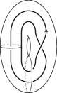
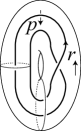
Put ℰ := S 3 ∖ Int N ( E ) assign ℰ superscript 𝑆 3 Int 𝑁 𝐸 \mathcal{E}:=S^{3}\setminus\operatorname{Int}{N(E)} ℱ := S 3 ∖ Int N ( E ( 2 , 2 b + 1 ) ) assign ℱ superscript 𝑆 3 Int 𝑁 superscript 𝐸 2 2 𝑏 1 \mathcal{F}:=S^{3}\setminus\operatorname{Int}{N(E^{(2,2b+1)})} L 𝐿 L D := D 2 × S 1 assign 𝐷 superscript 𝐷 2 superscript 𝑆 1 D:=D^{2}\times S^{1} 2 𝒞 := D ∖ Int N ( L ) assign 𝒞 𝐷 Int 𝑁 𝐿 \mathcal{C}:=D\setminus\operatorname{Int}{N(L)}
Figure 2. A knot L 𝐿 L
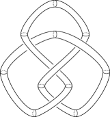
Then ℱ ℱ \mathcal{F} 𝒞 𝒞 \mathcal{C} ℰ ℰ \mathcal{E} ∂ D 2 × S 1 ⊂ ∂ D superscript 𝐷 2 superscript 𝑆 1 𝐷 \partial{D^{2}}\times S^{1}\subset\partial{D} ∂ ℰ ℰ \partial\mathcal{E} { point } × S 1 point superscript 𝑆 1 \{\text{point}\}\times S^{1} λ E μ E b subscript 𝜆 𝐸 superscript subscript 𝜇 𝐸 𝑏 \lambda_{E}\mu_{E}^{b} ( ∂ D 2 ) × { point } superscript 𝐷 2 point (\partial{}D^{2})\times\{\text{point}\} μ E subscript 𝜇 𝐸 \mu_{E} λ E ⊂ ∂ ℰ subscript 𝜆 𝐸 ℰ \lambda_{E}\subset\partial\mathcal{E} μ E ⊂ ∂ ℰ subscript 𝜇 𝐸 ℰ \mu_{E}\subset\partial\mathcal{E} E 𝐸 E 3
∪ \cup
Figure 3. ℱ ℱ \mathcal{F} ℰ ℰ \mathcal{E} L 𝐿 L
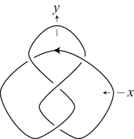
We calculate the fundamental group of S 3 ∖ E ( 2 , 2 b + 1 ) superscript 𝑆 3 superscript 𝐸 2 2 𝑏 1 S^{3}\setminus{E^{(2,2b+1)}} π 1 ( S 3 ∖ E ) subscript 𝜋 1 superscript 𝑆 3 𝐸 \pi_{1}(S^{3}\setminus{E}) π 1 ( ℰ ) subscript 𝜋 1 ℰ \pi_{1}(\mathcal{E}) π 1 ( S 3 ∖ E ( 2 , 2 b + 1 ) ) subscript 𝜋 1 superscript 𝑆 3 superscript 𝐸 2 2 𝑏 1 \pi_{1}(S^{3}\setminus{E^{(2,2b+1)}}) π 1 ( ℱ ) subscript 𝜋 1 ℱ \pi_{1}(\mathcal{F}) π 1 ( D ∖ L ) subscript 𝜋 1 𝐷 𝐿 \pi_{1}(D\setminus{L}) π 1 ( 𝒞 ) subscript 𝜋 1 𝒞 \pi_{1}(\mathcal{C}) ∂ ℰ ℰ \partial\mathcal{E} ∂ D 𝐷 \partial{D} 4 π 1 ( ℰ ) subscript 𝜋 1 ℰ \pi_{1}(\mathcal{E})
(4.1) ⟨ x , y ∣ x y − 1 x − 1 y x = y x y − 1 x − 1 y ⟩ . inner-product 𝑥 𝑦
𝑥 superscript 𝑦 1 superscript 𝑥 1 𝑦 𝑥 𝑦 𝑥 superscript 𝑦 1 superscript 𝑥 1 𝑦 \langle x,y\mid xy^{-1}x^{-1}yx=yxy^{-1}x^{-1}y\rangle.
Figure 4. Figure-eight knot E 𝐸 E
Since 𝒞 𝒞 \mathcal{C} ( 2 , 4 ) 2 4 (2,4) 5 π 1 ( 𝒞 ) subscript 𝜋 1 𝒞 \pi_{1}(\mathcal{C})
π 1 ( 𝒞 ) = ⟨ p , r ∣ p r p r = r p r p ⟩ , subscript 𝜋 1 𝒞 inner-product 𝑝 𝑟
𝑝 𝑟 𝑝 𝑟 𝑟 𝑝 𝑟 𝑝 \pi_{1}(\mathcal{C})=\langle p,r\mid prpr=rprp\rangle,
if we choose generators as in Figure 5
Figure 5. ( 2 , 4 ) 2 4 (2,4) 𝒞 𝒞 \mathcal{C}
Observe that the meridian of the solid torus D 𝐷 D p r p r − 1 𝑝 𝑟 𝑝 superscript 𝑟 1 prpr^{-1} ( 2 , 4 ) 2 4 (2,4) 5 λ E subscript 𝜆 𝐸 \lambda_{E} x y − 1 x y x − 2 y x y − 1 x − 1 𝑥 superscript 𝑦 1 𝑥 𝑦 superscript 𝑥 2 𝑦 𝑥 superscript 𝑦 1 superscript 𝑥 1 xy^{-1}xyx^{-2}yxy^{-1}x^{-1} S 3 ∖ E ( 2 , 2 b + 1 ) superscript 𝑆 3 superscript 𝐸 2 2 𝑏 1 S^{3}\setminus E^{(2,2b+1)}
π 1 ( ℱ ) = ⟨ x , y ∣ x y − 1 x − 1 y x = y x y − 1 x − 1 y ⟩ ⋃ r = λ E μ E b p r p r − 1 = μ E ⟨ p , r ∣ p r p r = r p r p ⟩ = ⟨ x , y , p , r ∣ x y − 1 x − 1 y x = y x y − 1 x − 1 y , p r p r = r p r p , x = p r p r − 1 , λ E = r x − b ⟩ , subscript 𝜋 1 ℱ inner-product 𝑥 𝑦
𝑥 superscript 𝑦 1 superscript 𝑥 1 𝑦 𝑥 𝑦 𝑥 superscript 𝑦 1 superscript 𝑥 1 𝑦 subscript 𝑟 subscript 𝜆 𝐸 superscript subscript 𝜇 𝐸 𝑏 𝑝 𝑟 𝑝 superscript 𝑟 1 subscript 𝜇 𝐸
inner-product 𝑝 𝑟
𝑝 𝑟 𝑝 𝑟 𝑟 𝑝 𝑟 𝑝 inner-product 𝑥 𝑦 𝑝 𝑟
formulae-sequence 𝑥 superscript 𝑦 1 superscript 𝑥 1 𝑦 𝑥 𝑦 𝑥 superscript 𝑦 1 superscript 𝑥 1 𝑦 formulae-sequence 𝑝 𝑟 𝑝 𝑟 𝑟 𝑝 𝑟 𝑝 formulae-sequence 𝑥 𝑝 𝑟 𝑝 superscript 𝑟 1 subscript 𝜆 𝐸 𝑟 superscript 𝑥 𝑏 \begin{split}&\pi_{1}(\mathcal{F})\\
=&\left\langle x,y\mid xy^{-1}x^{-1}yx=yxy^{-1}x^{-1}y\right\rangle\bigcup_{\begin{subarray}{c}r=\lambda_{E}\mu_{E}^{b}\\
prpr^{-1}=\mu_{E}\end{subarray}}\left\langle p,r\mid prpr=rprp\right\rangle\\
=&\left\langle x,y,p,r\mid xy^{-1}x^{-1}yx=yxy^{-1}x^{-1}y,prpr=rprp,x=prpr^{-1},\lambda_{E}=rx^{-b}\right\rangle,\end{split}
where λ E := x y − 1 x y x − 2 y x y − 1 x − 1 assign subscript 𝜆 𝐸 𝑥 superscript 𝑦 1 𝑥 𝑦 superscript 𝑥 2 𝑦 𝑥 superscript 𝑦 1 superscript 𝑥 1 \lambda_{E}:=xy^{-1}xyx^{-2}yxy^{-1}x^{-1} x 𝑥 x μ E subscript 𝜇 𝐸 \mu_{E} r 𝑟 r
For a complex number u 𝑢 u ρ u : π 1 ( ℱ ) → SL ( 2 ; ℂ ) : subscript 𝜌 𝑢 → subscript 𝜋 1 ℱ SL 2 ℂ
\rho_{u}\colon\pi_{1}(\mathcal{F})\to\mathrm{SL}(2;\mathbb{C}) ρ u | π 1 ( ℰ ) \rho_{u}\bigm{|}_{\pi_{1}(\mathcal{E})}
ρ u ( x ) subscript 𝜌 𝑢 𝑥 \displaystyle\rho_{u}(x) := ( e u 1 0 e − u ) , assign absent matrix superscript 𝑒 𝑢 1 0 superscript 𝑒 𝑢 \displaystyle:=\begin{pmatrix}e^{u}&1\\
0&e^{-u}\end{pmatrix},
ρ u ( y ) subscript 𝜌 𝑢 𝑦 \displaystyle\rho_{u}(y) := ( e u 0 − δ ( u ) e − u ) , assign absent matrix superscript 𝑒 𝑢 0 𝛿 𝑢 superscript 𝑒 𝑢 \displaystyle:=\begin{pmatrix}e^{u}&0\\
-\delta(u)&e^{-u}\end{pmatrix},
where
δ ( u ) := 1 2 ( e 2 u + e − 2 u − 3 + ( e 2 u + e − 2 u + 1 ) ( e 2 u + e − 2 u − 3 ) ) . assign 𝛿 𝑢 1 2 superscript 𝑒 2 𝑢 superscript 𝑒 2 𝑢 3 superscript 𝑒 2 𝑢 superscript 𝑒 2 𝑢 1 superscript 𝑒 2 𝑢 superscript 𝑒 2 𝑢 3 \delta(u):=\frac{1}{2}\left(e^{2u}+e^{-2u}-3+\sqrt{(e^{2u}+e^{-2u}+1)(e^{2u}+e^{-2u}-3)}\right).
Note that from [31 ] , any non-Abelian representation π 1 ( ℰ ) → SL ( 2 ; ℂ ) → subscript 𝜋 1 ℰ SL 2 ℂ
\pi_{1}(\mathcal{E})\to\mathrm{SL}(2;\mathbb{C}) λ E subscript 𝜆 𝐸 \lambda_{E} E 𝐸 E
ρ u ( λ E ) = ( ℓ ( u ) ( e u + e − u ) ( e 2 u + e − 2 u + 1 ) ( e 2 u + e − 2 u − 3 ) 0 ℓ ( u ) − 1 ) , subscript 𝜌 𝑢 subscript 𝜆 𝐸 matrix ℓ 𝑢 superscript 𝑒 𝑢 superscript 𝑒 𝑢 superscript 𝑒 2 𝑢 superscript 𝑒 2 𝑢 1 superscript 𝑒 2 𝑢 superscript 𝑒 2 𝑢 3 0 ℓ superscript 𝑢 1 \rho_{u}(\lambda_{E})=\begin{pmatrix}\ell(u)&(e^{u}+e^{-u})\sqrt{(e^{2u}+e^{-2u}+1)(e^{2u}+e^{-2u}-3)}\\
0&\ell(u)^{-1}\end{pmatrix},
where
ℓ ( u ) := 1 2 ( e 4 u − e 2 u − 2 − e − 2 u + e − 4 u ) + e 2 u − e − 2 u 2 ( e 2 u + e − 2 u + 1 ) ( e 2 u + e − 2 u − 3 ) . assign ℓ 𝑢 1 2 superscript 𝑒 4 𝑢 superscript 𝑒 2 𝑢 2 superscript 𝑒 2 𝑢 superscript 𝑒 4 𝑢 superscript 𝑒 2 𝑢 superscript 𝑒 2 𝑢 2 superscript 𝑒 2 𝑢 superscript 𝑒 2 𝑢 1 superscript 𝑒 2 𝑢 superscript 𝑒 2 𝑢 3 \ell(u)\\
:=\frac{1}{2}(e^{4u}-e^{2u}-2-e^{-2u}+e^{-4u})+\frac{e^{2u}-e^{-2u}}{2}\sqrt{(e^{2u}+e^{-2u}+1)(e^{2u}+e^{-2u}-3)}.
We extend it to π 1 ( ℱ ) subscript 𝜋 1 ℱ \pi_{1}(\mathcal{F}) π 1 ( 𝒞 ) subscript 𝜋 1 𝒞 \pi_{1}(\mathcal{C})
ρ u ( p ) = ( e u / 2 1 2 cosh ( u / 2 ) 0 e − u / 2 ) subscript 𝜌 𝑢 𝑝 matrix superscript 𝑒 𝑢 2 1 2 𝑢 2 0 superscript 𝑒 𝑢 2 \rho_{u}(p)=\begin{pmatrix}e^{u/2}&\frac{1}{2\cosh(u/2)}\\
0&e^{-u/2}\end{pmatrix}
so that ρ u ( p ) 2 = ρ u ( x ) subscript 𝜌 𝑢 superscript 𝑝 2 subscript 𝜌 𝑢 𝑥 \rho_{u}(p)^{2}=\rho_{u}(x)
ρ u ( x ) b = ( e b u e b u − e − b u e u − e − u 0 e − b u ) , subscript 𝜌 𝑢 superscript 𝑥 𝑏 matrix superscript 𝑒 𝑏 𝑢 superscript 𝑒 𝑏 𝑢 superscript 𝑒 𝑏 𝑢 superscript 𝑒 𝑢 superscript 𝑒 𝑢 0 superscript 𝑒 𝑏 𝑢 \rho_{u}(x)^{b}=\begin{pmatrix}e^{bu}&\frac{e^{bu}-e^{-bu}}{e^{u}-e^{-u}}\\
0&e^{-bu}\end{pmatrix},
we have
ρ u ( r ) = ρ u ( λ E ) ρ u ( x ) b = ( ℓ ( u ) e b u e b u ( e u + e − u ) ( e 2 u + e − 2 u + 1 ) ( e 2 u + e − 2 u − 3 ) + ℓ ( u ) − 1 e b u − e − b u e u − e − u 0 ℓ ( u ) − 1 e − b u ) . subscript 𝜌 𝑢 𝑟 subscript 𝜌 𝑢 subscript 𝜆 𝐸 subscript 𝜌 𝑢 superscript 𝑥 𝑏 matrix ℓ 𝑢 superscript 𝑒 𝑏 𝑢 superscript 𝑒 𝑏 𝑢 superscript 𝑒 𝑢 superscript 𝑒 𝑢 superscript 𝑒 2 𝑢 superscript 𝑒 2 𝑢 1 superscript 𝑒 2 𝑢 superscript 𝑒 2 𝑢 3 ℓ superscript 𝑢 1 superscript 𝑒 𝑏 𝑢 superscript 𝑒 𝑏 𝑢 superscript 𝑒 𝑢 superscript 𝑒 𝑢 0 ℓ superscript 𝑢 1 superscript 𝑒 𝑏 𝑢 \begin{split}\rho_{u}(r)&=\rho_{u}(\lambda_{E})\rho_{u}(x)^{b}\\
&=\begin{pmatrix}\ell(u)e^{bu}&e^{bu}(e^{u}+e^{-u})\sqrt{(e^{2u}+e^{-2u}+1)(e^{2u}+e^{-2u}-3)}+\ell(u)^{-1}\frac{e^{bu}-e^{-bu}}{e^{u}-e^{-u}}\\
0&\ell(u)^{-1}e^{-bu}\end{pmatrix}.\end{split}
We can see that ρ u ( p ) subscript 𝜌 𝑢 𝑝 \rho_{u}(p) ρ u ( r ) subscript 𝜌 𝑢 𝑟 \rho_{u}(r) ρ u subscript 𝜌 𝑢 \rho_{u}
Remark 4.1 .
Note that δ ( κ ) = 0 𝛿 𝜅 0 \delta(\kappa)=0 e 2 κ = 3 + 5 2 superscript 𝑒 2 𝜅 3 5 2 e^{2\kappa}=\frac{3+\sqrt{5}}{2} t − 3 + t − 1 𝑡 3 superscript 𝑡 1 t-3+t^{-1} e κ superscript 𝑒 𝜅 e^{\kappa} E ( 2 , 2 b + 1 ) superscript 𝐸 2 2 𝑏 1 E^{(2,2b+1)}
Δ ( E ( 2 , 2 b + 1 ) ; t ) = ( − t 2 + 3 − t − 2 ) × t ( 2 b + 1 ) / 2 + t − ( 2 b + 1 ) / 2 t 1 / 2 + t − 1 / 2 . Δ superscript 𝐸 2 2 𝑏 1 𝑡
superscript 𝑡 2 3 superscript 𝑡 2 superscript 𝑡 2 𝑏 1 2 superscript 𝑡 2 𝑏 1 2 superscript 𝑡 1 2 superscript 𝑡 1 2 \Delta(E^{(2,2b+1)};t)=(-t^{2}+3-t^{-2})\times\frac{t^{(2b+1)/2}+t^{-(2b+1)/2}}{t^{1/2}+t^{-1/2}}.
The preferred longitude λ 𝜆 \lambda E ( 2 , 2 b + 1 ) superscript 𝐸 2 2 𝑏 1 E^{(2,2b+1)} E 𝐸 E ρ u | π 1 ( 𝒞 ) \rho_{u}\bigm{|}_{\pi_{1}(\mathcal{C})}
ρ u ( λ ) = ρ u ( λ E ) 2 = ( ℓ ( u ) 2 ∗ 0 ℓ ( u ) − 2 ) . subscript 𝜌 𝑢 𝜆 subscript 𝜌 𝑢 superscript subscript 𝜆 𝐸 2 matrix ℓ superscript 𝑢 2 ∗ 0 ℓ superscript 𝑢 2 \rho_{u}(\lambda)=\rho_{u}(\lambda_{E})^{2}=\begin{pmatrix}\ell(u)^{2}&\ast\\
0&\ell(u)^{-2}\end{pmatrix}.
Remark 4.2 .
The function ℓ ( u ) ℓ 𝑢 \ell(u)
(4.2) ℓ ( u ) − ( e 4 u − e 2 u − 2 − e − 2 u + e − 4 u ) + ℓ ( u ) − 1 = 0 , ℓ 𝑢 superscript 𝑒 4 𝑢 superscript 𝑒 2 𝑢 2 superscript 𝑒 2 𝑢 superscript 𝑒 4 𝑢 ℓ superscript 𝑢 1 0 \ell(u)-(e^{4u}-e^{2u}-2-e^{-2u}+e^{-4u})+\ell(u)^{-1}=0,
and so ℓ ( u ) 2 ℓ superscript 𝑢 2 \ell(u)^{2}
(4.3) ℓ ( u ) 2 + ℓ ( u ) − 2 = ( e 4 u − e 2 u − 2 − e − 2 u + e − 4 u ) 2 − 2 . ℓ superscript 𝑢 2 ℓ superscript 𝑢 2 superscript superscript 𝑒 4 𝑢 superscript 𝑒 2 𝑢 2 superscript 𝑒 2 𝑢 superscript 𝑒 4 𝑢 2 2 \ell(u)^{2}+\ell(u)^{-2}=\left(e^{4u}-e^{2u}-2-e^{-2u}+e^{-4u}\right)^{2}-2.
Compare them with the A-polynomial of the figure-eight knot ([1 , Appendix] )
𝔩 − ( 𝔪 4 − 𝔪 2 − 2 − 𝔪 − 2 + 𝔪 − 4 ) + 𝔩 − 1 𝔩 superscript 𝔪 4 superscript 𝔪 2 2 superscript 𝔪 2 superscript 𝔪 4 superscript 𝔩 1 \mathfrak{l}-(\mathfrak{m}^{4}-\mathfrak{m}^{2}-2-\mathfrak{m}^{-2}+\mathfrak{m}^{-4})+\mathfrak{l}^{-1}
and the A-polynomial of E ( 2 , 2 b + 1 ) superscript 𝐸 2 2 𝑏 1 E^{(2,2b+1)} [28 , Example 2.11] ) given by
( 1 + 𝔪 2 ( 2 b + 1 ) 𝔩 ) ( 𝔩 − ( 𝔪 8 − 𝔪 4 − 2 − 𝔪 − 4 + 𝔪 − 8 ) 2 − 2 + 𝔩 − 1 ) . 1 superscript 𝔪 2 2 𝑏 1 𝔩 𝔩 superscript superscript 𝔪 8 superscript 𝔪 4 2 superscript 𝔪 4 superscript 𝔪 8 2 2 superscript 𝔩 1 \left(1+\mathfrak{m}^{2(2b+1)}\mathfrak{l}\right)\left(\mathfrak{l}-\left(\mathfrak{m}^{8}-\mathfrak{m}^{4}-2-\mathfrak{m}^{-4}+\mathfrak{m}^{-8}\right)^{2}-2+\mathfrak{l}^{-1}\right).
Note that the meridian of E 𝐸 E E ( 2 , 2 b + 1 ) superscript 𝐸 2 2 𝑏 1 E^{(2,2b+1)} x = p 2 𝑥 superscript 𝑝 2 x=p^{2} p 𝑝 p
Remark 4.3 .
If we use the hyperbolic functions, we have the following expressions for ℓ ( u ) ℓ 𝑢 \ell(u)
ℓ ( u ) ℓ 𝑢 \displaystyle\ell(u) = cosh ( 4 u ) − cosh ( 2 u ) − 1 + sinh ( 2 u ) ( 2 cosh ( 2 u ) + 1 ) ( 2 cosh ( 2 u ) − 3 ) absent 4 𝑢 2 𝑢 1 2 𝑢 2 2 𝑢 1 2 2 𝑢 3 \displaystyle=\cosh(4u)-\cosh(2u)-1+\sinh(2u)\sqrt{(2\cosh(2u)+1)(2\cosh(2u)-3)}
= 2 cosh 2 ( 2 u ) − cosh ( 2 u ) − 2 + sinh ( 2 u ) ( 2 cosh ( 2 u ) + 1 ) ( 2 cosh ( 2 u ) − 3 ) absent 2 superscript 2 2 𝑢 2 𝑢 2 2 𝑢 2 2 𝑢 1 2 2 𝑢 3 \displaystyle=2\cosh^{2}(2u)-\cosh(2u)-2+\sinh(2u)\sqrt{(2\cosh(2u)+1)(2\cosh(2u)-3)}
= cosh ( 4 u ) − cosh ( 2 u ) − 1 + 2 sinh ( 2 u ) sinh φ ( u ) . absent 4 𝑢 2 𝑢 1 2 2 𝑢 𝜑 𝑢 \displaystyle=\cosh(4u)-\cosh(2u)-1+2\sinh(2u)\sinh\varphi(u).
Here the last equality follows since cosh φ ( u ) = cosh ( 2 u ) − 1 2 𝜑 𝑢 2 𝑢 1 2 \cosh\varphi(u)=\cosh(2u)-\frac{1}{2}
Since cosh ( 2 κ ) = 3 2 2 𝜅 3 2 \cosh(2\kappa)=\frac{3}{2}
ℓ ( κ ) = 1 . ℓ 𝜅 1 \ell(\kappa)=1.
For u 𝑢 u κ 𝜅 \kappa
Lemma 4.4 .
If u > κ 𝑢 𝜅 u>\kappa ℓ ( u ) ℓ 𝑢 \ell(u) ℓ ( u ) > 1 ℓ 𝑢 1 \ell(u)>1
Proof.
Since cosh ( 2 u ) > 3 2 2 𝑢 3 2 \cosh(2u)>\frac{3}{2} u > κ 𝑢 𝜅 u>\kappa ℓ ( u ) ℓ 𝑢 \ell(u)
ℓ ( u ) > 2 cosh 2 ( 2 u ) − cosh ( 2 u ) − 2 > 1 . ℓ 𝑢 2 superscript 2 2 𝑢 2 𝑢 2 1 \ell(u)>2\cosh^{2}(2u)-\cosh(2u)-2>1.
∎
Remark 4.5 .
If u 𝑢 u u > κ 𝑢 𝜅 u>\kappa ρ u subscript 𝜌 𝑢 \rho_{u} SL ( 2 ; ℝ ) SL 2 ℝ
\mathrm{SL}(2;\mathbb{R})
5. Chern–Simons invariant
We will calculate the PSL ( 2 ; ℂ ) PSL 2 ℂ
\mathrm{PSL}(2;\mathbb{C}) ℱ ℱ \mathcal{F} ρ u subscript 𝜌 𝑢 \rho_{u}
A practical definition of the Chern–Simons invariant is as follows.
See [17 ] for the precise definition.
Let M 𝑀 M ∂ M 𝑀 \partial{M}
The PSL ( 2 ; ℂ ) PSL 2 ℂ
\mathrm{PSL}(2;\mathbb{C}) X ( ∂ M ) 𝑋 𝑀 X(\partial{M}) π 1 ( ∂ M ) subscript 𝜋 1 𝑀 \pi_{1}(\partial{M}) Hom ( π 1 ( ∂ ) , PSL ( 2 ; ℂ ) ) Hom subscript 𝜋 1 PSL 2 ℂ
\operatorname{Hom}(\pi_{1}(\partial),\mathrm{PSL}(2;\mathbb{C})) { μ , λ } 𝜇 𝜆 \{\mu,\lambda\} π 1 ( ∂ M ) ≅ ℤ 2 subscript 𝜋 1 𝑀 superscript ℤ 2 \pi_{1}(\partial{M})\cong\mathbb{Z}^{2} ∂ M 𝑀 \partial{M} PSL ( 2 ; ℂ ) PSL 2 ℂ
\mathrm{PSL}(2;\mathbb{C}) γ 𝛾 \gamma
γ ( μ ) 𝛾 𝜇 \displaystyle\gamma(\mu) = ± ( e 2 π − 1 g ( γ ) ∗ 0 e − 2 π − 1 g ( γ ) ) , absent plus-or-minus matrix superscript 𝑒 2 𝜋 1 𝑔 𝛾 ∗ 0 superscript 𝑒 2 𝜋 1 𝑔 𝛾 \displaystyle=\pm\begin{pmatrix}e^{2\pi\sqrt{-1}g(\gamma)}&\ast\\
0&e^{-2\pi\sqrt{-1}g(\gamma)}\end{pmatrix},
γ ( λ ) 𝛾 𝜆 \displaystyle\gamma(\lambda) = ± ( e 2 π − 1 h ( γ ) ∗ 0 e − 2 π − 1 h ( γ ) ) absent plus-or-minus matrix superscript 𝑒 2 𝜋 1 ℎ 𝛾 ∗ 0 superscript 𝑒 2 𝜋 1 ℎ 𝛾 \displaystyle=\pm\begin{pmatrix}e^{2\pi\sqrt{-1}h(\gamma)}&\ast\\
0&e^{-2\pi\sqrt{-1}h(\gamma)}\end{pmatrix}
after suitable conjugation.
Then the map γ ↦ ( g ( γ ) , h ( γ ) ) maps-to 𝛾 𝑔 𝛾 ℎ 𝛾 \gamma\mapsto(g(\gamma),h(\gamma)) X ( ∂ M ) 𝑋 𝑀 X(\partial{M}) ℂ 2 / H superscript ℂ 2 𝐻 \mathbb{C}^{2}/H H 𝐻 H
H := ⟨ X , Y , b ∣ [ X , Y ] = X b X b = Y b Y b = b 2 = 1 ⟩ , assign 𝐻 inner-product 𝑋 𝑌 𝑏
𝑋 𝑌 𝑋 𝑏 𝑋 𝑏 𝑌 𝑏 𝑌 𝑏 superscript 𝑏 2 1 H:=\langle X,Y,b\mid[X,Y]=XbXb=YbYb=b^{2}=1\rangle,
and it acts on ℂ 2 superscript ℂ 2 \mathbb{C}^{2}
X ⋅ ( x , y ) ⋅ 𝑋 𝑥 𝑦 \displaystyle X\cdot(x,y) := ( x + 1 2 , y ) , assign absent 𝑥 1 2 𝑦 \displaystyle:=\left(x+\frac{1}{2},y\right),
Y ⋅ ( x , y ) ⋅ 𝑌 𝑥 𝑦 \displaystyle Y\cdot(x,y) := ( x , y + 1 2 ) , assign absent 𝑥 𝑦 1 2 \displaystyle:=\left(x,y+\frac{1}{2}\right),
b ⋅ ( x , y ) ⋅ 𝑏 𝑥 𝑦 \displaystyle b\cdot(x,y) = ( − x , − y ) . absent 𝑥 𝑦 \displaystyle=(-x,-y).
We define E ( ∂ M ) 𝐸 𝑀 E(\partial{M}) ℂ 2 × ℂ × superscript ℂ 2 superscript ℂ \mathbb{C}^{2}\times\mathbb{C}^{\times} H 𝐻 H H 𝐻 H E ( ∂ M ) 𝐸 𝑀 E(\partial{M})
X ⋅ ( x , y ; z ) ⋅ 𝑋 𝑥 𝑦 𝑧 \displaystyle X\cdot(x,y;z) := ( x + 1 2 , y ; z × e − 4 y π − 1 ) , assign absent 𝑥 1 2 𝑦 𝑧 superscript 𝑒 4 𝑦 𝜋 1 \displaystyle:=\left(x+\frac{1}{2},y;z\times e^{-4y\pi\sqrt{-1}}\right),
Y ⋅ ( x , y ; z ) ⋅ 𝑌 𝑥 𝑦 𝑧 \displaystyle Y\cdot(x,y;z) := ( x , y + 1 2 ; z × e 4 x π − 1 ) , assign absent 𝑥 𝑦 1 2 𝑧 superscript 𝑒 4 𝑥 𝜋 1 \displaystyle:=\left(x,y+\frac{1}{2};z\times e^{4x\pi\sqrt{-1}}\right),
b ⋅ ( x , y ; z ) ⋅ 𝑏 𝑥 𝑦 𝑧 \displaystyle b\cdot(x,y;z) := ( − x , − y ; z ) . assign absent 𝑥 𝑦 𝑧 \displaystyle:=(-x,-y;z).
We denote by [ x , y ; z ] ∈ E ( ∂ M ) 𝑥 𝑦 𝑧
𝐸 𝑀 [x,y;z]\in E(\partial{M}) ( x , y , z ) 𝑥 𝑦 𝑧 (x,y,z)
(5.1) { [ x , y ; z ] = [ x + 1 2 , y ; z × e − 4 y π − 1 ] , [ x , y ; z ] = [ x , y + 1 2 ; z × e 4 x π − 1 ] , [ x , y ; z ] = [ − x , − y ; z ] . cases 𝑥 𝑦 𝑧
absent 𝑥 1 2 𝑦 𝑧 superscript 𝑒 4 𝑦 𝜋 1
𝑥 𝑦 𝑧
absent 𝑥 𝑦 1 2 𝑧 superscript 𝑒 4 𝑥 𝜋 1
𝑥 𝑦 𝑧
absent 𝑥 𝑦 𝑧
\begin{cases}[x,y;z]&=\left[x+\frac{1}{2},y;z\times e^{-4y\pi\sqrt{-1}}\right],\\[8.53581pt]
[x,y;z]&=\left[x,y+\frac{1}{2};z\times e^{4x\pi\sqrt{-1}}\right],\\[8.53581pt]
[x,y;z]&=[-x,-y;z].\end{cases}
Then we can see that q : E ( ∂ M ) → X ( ∂ M ) : 𝑞 → 𝐸 𝑀 𝑋 𝑀 q\colon E(\partial{M})\to X(\partial{M}) q : [ x , y ; z ] ↦ [ x , y ] : 𝑞 maps-to 𝑥 𝑦 𝑧
𝑥 𝑦 q\colon[x,y;z]\mapsto[x,y] ℂ × superscript ℂ \mathbb{C}^{\times}
Now the Chern–Simons function cs M subscript cs 𝑀 \operatorname{cs}_{M} PSL ( 2 , ℂ ) PSL 2 ℂ \mathrm{PSL}(2,\mathbb{C}) X ( M ) 𝑋 𝑀 X(M) π 1 ( M ) subscript 𝜋 1 𝑀 \pi_{1}(M) E ( ∂ M ) 𝐸 𝑀 E(\partial{M})
E ( ∂ M ) 𝐸 𝑀 {E(\partial{M})} X ( M ) 𝑋 𝑀 {X(M)} X ( ∂ M ) . 𝑋 𝑀 {X(\partial{M}).} q 𝑞 \scriptstyle{q} cs M subscript cs 𝑀 \scriptstyle{\operatorname{cs}_{M}} r 𝑟 \scriptstyle{r}
Here r : X ( M ) → X ( ∂ M ) : 𝑟 → 𝑋 𝑀 𝑋 𝑀 r\colon X(M)\to X(\partial{M})
Definition 5.1 .
If cs M ( [ γ ] ) = [ u 4 π − 1 , v 4 π − 1 ; z ] subscript cs 𝑀 delimited-[] 𝛾 𝑢 4 𝜋 1 𝑣 4 𝜋 1 𝑧
\operatorname{cs}_{M}([\gamma])=\left[\frac{u}{4\pi\sqrt{-1}},\frac{v}{4\pi\sqrt{-1}};z\right] CS M ( [ γ ] ; u , v ) := π − 1 2 log z ( mod π 2 ℤ ) assign subscript CS 𝑀 delimited-[] 𝛾 𝑢 𝑣 annotated 𝜋 1 2 𝑧 pmod superscript 𝜋 2 ℤ \operatorname{CS}_{M}([\gamma];u,v):=\frac{\pi\sqrt{-1}}{2}\log{z}\pmod{\pi^{2}\mathbb{Z}} M 𝑀 M [ γ ] delimited-[] 𝛾 [\gamma] ( u 4 π − 1 , v 4 π − 1 ) 𝑢 4 𝜋 1 𝑣 4 𝜋 1 \left(\frac{u}{4\pi\sqrt{-1}},\frac{v}{4\pi\sqrt{-1}}\right) X ( ∂ M ) 𝑋 𝑀 X(\partial{M}) [ γ ] ∈ X ( M ) delimited-[] 𝛾 𝑋 𝑀 [\gamma]\in X(M) γ 𝛾 \gamma
To calculate the Chern–Simons invariant, we use the following theorem of Kirk and Klassen [17 ] .
Theorem 5.2 (Kirk–Klassen).
Let M 𝑀 M ∂ M 𝑀 \partial M γ t : π 1 ( M ) → PSL ( 2 ; ℂ ) : subscript 𝛾 𝑡 → subscript 𝜋 1 𝑀 PSL 2 ℂ
\gamma_{t}\colon\pi_{1}(M)\to\mathrm{PSL}(2;\mathbb{C})
γ t ( μ M ) subscript 𝛾 𝑡 subscript 𝜇 𝑀 \displaystyle\gamma_{t}(\mu_{M}) = ( e u ( t ) / 2 ∗ 0 e − u ( t ) / 2 ) , absent matrix superscript 𝑒 𝑢 𝑡 2 ∗ 0 superscript 𝑒 𝑢 𝑡 2 \displaystyle=\begin{pmatrix}e^{u(t)/2}&\ast\\
0&e^{-u(t)/2}\end{pmatrix},
γ t ( λ M ) subscript 𝛾 𝑡 subscript 𝜆 𝑀 \displaystyle\gamma_{t}(\lambda_{M}) = ( e v ( t ) / 2 ∗ 0 e − v ( t ) / 2 ) absent matrix superscript 𝑒 𝑣 𝑡 2 ∗ 0 superscript 𝑒 𝑣 𝑡 2 \displaystyle=\begin{pmatrix}e^{v(t)/2}&\ast\\
0&e^{-v(t)/2}\end{pmatrix}
up to conjugation, where μ M , λ M ∈ π 1 ( ∂ M ) subscript 𝜇 𝑀 subscript 𝜆 𝑀
subscript 𝜋 1 𝑀 \mu_{M},\lambda_{M}\in\pi_{1}(\partial{M}) ∂ M 𝑀 \partial{M}
If cs M ( [ ρ t ] ) = [ u ( t ) 4 π − 1 , v ( t ) 4 π − 1 ; z ( t ) ] subscript cs 𝑀 delimited-[] subscript 𝜌 𝑡 𝑢 𝑡 4 𝜋 1 𝑣 𝑡 4 𝜋 1 𝑧 𝑡
\operatorname{cs}_{M}([\rho_{t}])=\left[\frac{u(t)}{4\pi\sqrt{-1}},\frac{v(t)}{4\pi\sqrt{-1}};z(t)\right]
z ( 1 ) z ( 0 ) = exp ( − 1 2 π ∫ 0 1 ( u ( t ) d v ( t ) d t − d u ( t ) d t v ( t ) ) 𝑑 t ) . 𝑧 1 𝑧 0 1 2 𝜋 superscript subscript 0 1 𝑢 𝑡 𝑑 𝑣 𝑡 𝑑 𝑡 𝑑 𝑢 𝑡 𝑑 𝑡 𝑣 𝑡 differential-d 𝑡 \frac{z(1)}{z(0)}=\exp\left(\frac{\sqrt{-1}}{2\pi}\int_{0}^{1}\bigl{(}u(t)\frac{d\,v(t)}{d\,t}-\frac{d\,u(t)}{d\,t}v(t)\bigr{)}\,dt\right).
We calculate the Chern–Simons invariant of ℱ ℱ \mathcal{F} 5.2
Putting u t := ( u − κ ) t + κ assign subscript 𝑢 𝑡 𝑢 𝜅 𝑡 𝜅 u_{t}:=(u-\kappa)t+\kappa α t subscript 𝛼 𝑡 \alpha_{t} β t subscript 𝛽 𝑡 \beta_{t} 0 ≤ t ≤ 1 0 𝑡 1 0\leq t\leq 1
α t subscript 𝛼 𝑡 \displaystyle\alpha_{t} : p ↦ ( e t κ / 2 0 0 e − t κ / 2 ) , x ↦ ( e t κ 0 0 e − t κ ) , y ↦ ( e t κ 0 0 e − t κ ) , : absent formulae-sequence maps-to 𝑝 matrix superscript 𝑒 𝑡 𝜅 2 0 0 superscript 𝑒 𝑡 𝜅 2 formulae-sequence maps-to 𝑥 matrix superscript 𝑒 𝑡 𝜅 0 0 superscript 𝑒 𝑡 𝜅 maps-to 𝑦 matrix superscript 𝑒 𝑡 𝜅 0 0 superscript 𝑒 𝑡 𝜅 \displaystyle\colon p\mapsto\begin{pmatrix}e^{t\kappa/2}&0\\
0&e^{-t\kappa/2}\end{pmatrix},\quad x\mapsto\begin{pmatrix}e^{t\kappa}&0\\
0&e^{-t\kappa}\end{pmatrix},\quad y\mapsto\begin{pmatrix}e^{t\kappa}&0\\
0&e^{-t\kappa}\end{pmatrix},
β t subscript 𝛽 𝑡 \displaystyle\beta_{t} : p ↦ ( e u t / 2 1 2 cosh ( u t / 2 ) 0 e − u t / 2 ) , x ↦ ( e u t 1 0 e − u t ) , y ↦ ( e u t 0 − d ( u t ) e − u t ) . : absent formulae-sequence maps-to 𝑝 matrix superscript 𝑒 subscript 𝑢 𝑡 2 1 2 subscript 𝑢 𝑡 2 0 superscript 𝑒 subscript 𝑢 𝑡 2 formulae-sequence maps-to 𝑥 matrix superscript 𝑒 subscript 𝑢 𝑡 1 0 superscript 𝑒 subscript 𝑢 𝑡 maps-to 𝑦 matrix superscript 𝑒 subscript 𝑢 𝑡 0 𝑑 subscript 𝑢 𝑡 superscript 𝑒 subscript 𝑢 𝑡 \displaystyle\colon p\mapsto\begin{pmatrix}e^{u_{t}/2}&\frac{1}{2\cosh(u_{t}/2)}\\
0&e^{-u_{t}/2}\end{pmatrix},x\mapsto\begin{pmatrix}e^{u_{t}}&1\\
0&e^{-u_{t}}\end{pmatrix},\quad y\mapsto\begin{pmatrix}e^{u_{t}}&0\\
-d(u_{t})&e^{-u_{t}}\end{pmatrix}.
Note that α 1 subscript 𝛼 1 \alpha_{1} β 0 subscript 𝛽 0 \beta_{0} β 0 subscript 𝛽 0 \beta_{0}
We can write
cs ℱ ( [ α t ] ) subscript cs ℱ delimited-[] subscript 𝛼 𝑡 \displaystyle\operatorname{cs}_{\mathcal{F}}([\alpha_{t}]) := [ t κ 4 π − 1 , 0 ; z ( t ) ] , assign absent 𝑡 𝜅 4 𝜋 1 0 𝑧 𝑡
\displaystyle:=\left[\frac{t\kappa}{4\pi\sqrt{-1}},0;z(t)\right],
cs ℱ ( [ β t ] ) subscript cs ℱ delimited-[] subscript 𝛽 𝑡 \displaystyle\operatorname{cs}_{\mathcal{F}}([\beta_{t}]) := [ u t 4 π − 1 , 4 log ℓ ( u t ) 4 π − 1 ; w ( t ) ] , assign absent subscript 𝑢 𝑡 4 𝜋 1 4 ℓ subscript 𝑢 𝑡 4 𝜋 1 𝑤 𝑡
\displaystyle:=\left[\frac{u_{t}}{4\pi\sqrt{-1}},\frac{4\log\ell(u_{t})}{4\pi\sqrt{-1}};w(t)\right],
since
α t ( λ ) subscript 𝛼 𝑡 𝜆 \displaystyle\alpha_{t}(\lambda) = ( 1 0 0 1 ) , absent matrix 1 0 0 1 \displaystyle=\begin{pmatrix}1&0\\
0&1\end{pmatrix},
β t ( λ ) subscript 𝛽 𝑡 𝜆 \displaystyle\beta_{t}(\lambda) = ( ℓ ( u t ) 2 ∗ 0 ℓ ( u t ) − 2 ) . absent matrix ℓ superscript subscript 𝑢 𝑡 2 ∗ 0 ℓ superscript subscript 𝑢 𝑡 2 \displaystyle=\begin{pmatrix}\ell(u_{t})^{2}&\ast\\
0&\ell(u_{t})^{-2}\end{pmatrix}.
Note that since ℓ ( u t ) > 1 ℓ subscript 𝑢 𝑡 1 \ell(u_{t})>1 4.4 log ℓ ( u t ) > 0 ℓ subscript 𝑢 𝑡 0 \log\ell(u_{t})>0 z ( 1 ) = z ( 0 ) = 1 𝑧 1 𝑧 0 1 z(1)=z(0)=1
w ( 1 ) w ( 0 ) = exp ( − 1 2 π ∫ 0 1 ( u t × 4 d log ℓ ( u t ) d t − 4 log ℓ ( u t ) × d u t d t ) 𝑑 t ) = exp ( 2 − 1 π ( [ u t log ℓ ( u t ) ] 0 1 − 2 ( u − κ ) ∫ 0 1 log ℓ ( u t ) 𝑑 t ) ) (putting s := u t ) = exp ( 2 − 1 π ( u log ℓ ( u ) − 2 ∫ κ u log ℓ ( s ) 𝑑 s ) ) . 𝑤 1 𝑤 0 1 2 𝜋 superscript subscript 0 1 subscript 𝑢 𝑡 4 𝑑 ℓ subscript 𝑢 𝑡 𝑑 𝑡 4 ℓ subscript 𝑢 𝑡 𝑑 subscript 𝑢 𝑡 𝑑 𝑡 differential-d 𝑡 2 1 𝜋 superscript subscript delimited-[] subscript 𝑢 𝑡 ℓ subscript 𝑢 𝑡 0 1 2 𝑢 𝜅 superscript subscript 0 1 ℓ subscript 𝑢 𝑡 differential-d 𝑡 (putting s := u t ) 2 1 𝜋 𝑢 ℓ 𝑢 2 superscript subscript 𝜅 𝑢 ℓ 𝑠 differential-d 𝑠 \begin{split}&\frac{w(1)}{w(0)}\\
=&\exp\left(\frac{\sqrt{-1}}{2\pi}\int_{0}^{1}\left(u_{t}\times\frac{4d\,\log\ell(u_{t})}{d\,t}-4\log\ell(u_{t})\times\frac{d\,u_{t}}{d\,t}\right)\,dt\right)\\
=&\exp\left(\frac{2\sqrt{-1}}{\pi}\left(\Bigl{[}u_{t}\log\ell(u_{t})\Bigr{]}_{0}^{1}-2(u-\kappa)\int_{0}^{1}\log\ell(u_{t})\,dt\right)\right)\\
&\quad\text{(putting $s:=u_{t}$)}\\
=&\exp\left(\frac{2\sqrt{-1}}{\pi}\left(u\log\ell(u)-2\int_{\kappa}^{u}\log\ell(s)\,ds\right)\right).\end{split}
Because α 1 subscript 𝛼 1 \alpha_{1} β 0 subscript 𝛽 0 \beta_{0} cs ℱ ( [ α 1 ] ) = cs ℱ ( [ β 0 ] ) subscript cs ℱ delimited-[] subscript 𝛼 1 subscript cs ℱ delimited-[] subscript 𝛽 0 \operatorname{cs}_{\mathcal{F}}([\alpha_{1}])=\operatorname{cs}_{\mathcal{F}}([\beta_{0}])
cs ℱ ( [ α 1 ] ) subscript cs ℱ delimited-[] subscript 𝛼 1 \displaystyle\operatorname{cs}_{\mathcal{F}}([\alpha_{1}]) = [ κ 4 π − 1 , 0 ; 1 ] , absent 𝜅 4 𝜋 1 0 1
\displaystyle=\left[\frac{\kappa}{4\pi\sqrt{-1}},0;1\right], and
cs ℱ ( β 0 ) subscript cs ℱ subscript 𝛽 0 \displaystyle\operatorname{cs}_{\mathcal{F}}(\beta_{0}) = [ κ 4 π − 1 , 4 log ℓ ( κ ) 4 π − 1 ; w ( 0 ) ] , absent 𝜅 4 𝜋 1 4 ℓ 𝜅 4 𝜋 1 𝑤 0
\displaystyle=\left[\frac{\kappa}{4\pi\sqrt{-1}},\frac{4\log\ell(\kappa)}{4\pi\sqrt{-1}};w(0)\right],
we have
[ κ 4 π − 1 , 0 ; 1 ] = [ κ 4 π − 1 , 4 log ℓ ( κ ) 4 π − 1 ; w ( 0 ) ] = [ κ 4 π − 1 , 0 ; w ( 0 ) ] 𝜅 4 𝜋 1 0 1
𝜅 4 𝜋 1 4 ℓ 𝜅 4 𝜋 1 𝑤 0
𝜅 4 𝜋 1 0 𝑤 0
\left[\frac{\kappa}{4\pi\sqrt{-1}},0;1\right]=\left[\frac{\kappa}{4\pi\sqrt{-1}},\frac{4\log\ell(\kappa)}{4\pi\sqrt{-1}};w(0)\right]=\left[\frac{\kappa}{4\pi\sqrt{-1}},0;w(0)\right]
since ℓ ( κ ) = 1 ℓ 𝜅 1 \ell(\kappa)=1 w ( 0 ) = 1 𝑤 0 1 w(0)=1
Therefore we have
w ( 1 ) = exp ( 2 − 1 π ( u log ℓ ( u ) − 2 ∫ κ u log ℓ ( s ) 𝑑 s ) ) 𝑤 1 2 1 𝜋 𝑢 ℓ 𝑢 2 superscript subscript 𝜅 𝑢 ℓ 𝑠 differential-d 𝑠 w(1)=\exp\left(\frac{2\sqrt{-1}}{\pi}\left(u\log\ell(u)-2\int_{\kappa}^{u}\log\ell(s)\,ds\right)\right)
and so
CS ℱ ( [ ρ u ] ; u , v ( u ) ) = 2 ∫ κ u log ℓ ( s ) 𝑑 s − u log ℓ ( u ) , subscript CS ℱ delimited-[] subscript 𝜌 𝑢 𝑢 𝑣 𝑢 2 superscript subscript 𝜅 𝑢 ℓ 𝑠 differential-d 𝑠 𝑢 ℓ 𝑢 \operatorname{CS}_{\mathcal{F}}\bigl{(}[\rho_{u}];u,v(u)\bigr{)}=2\int_{\kappa}^{u}\log\ell(s)\,ds-u\log\ell(u),
if we put v ( u ) := 4 log ℓ ( u ) assign 𝑣 𝑢 4 ℓ 𝑢 v(u):=4\log\ell(u)
Now we put
S ( u ) := Li 2 ( e − φ ( u ) − 2 u ) − Li 2 ( e φ ( u ) − 2 u ) + 2 u φ ( u ) . assign 𝑆 𝑢 subscript Li 2 superscript 𝑒 𝜑 𝑢 2 𝑢 subscript Li 2 superscript 𝑒 𝜑 𝑢 2 𝑢 2 𝑢 𝜑 𝑢 S(u):=\operatorname{Li}_{2}(e^{-\varphi(u)-2u})-\operatorname{Li}_{2}(e^{\varphi(u)-2u})+2u\varphi(u).
We will show that CS ℱ ( [ ρ u ] ; u , v ( u ) ) = S ( u ) − u log ℓ ( u ) subscript CS ℱ delimited-[] subscript 𝜌 𝑢 𝑢 𝑣 𝑢 𝑆 𝑢 𝑢 ℓ 𝑢 \operatorname{CS}_{\mathcal{F}}\bigl{(}[\rho_{u}];u,v(u)\bigr{)}=S(u)-u\log\ell(u)
(5.2) S ( u ) = 2 ∫ κ u log ℓ ( s ) 𝑑 s . 𝑆 𝑢 2 superscript subscript 𝜅 𝑢 ℓ 𝑠 differential-d 𝑠 S(u)=2\int_{\kappa}^{u}\log\ell(s)\,ds.
Since e φ ( u ) + e − φ ( u ) = e 2 u + e − 2 u − 1 = 2 cosh ( 2 u ) − 1 superscript 𝑒 𝜑 𝑢 superscript 𝑒 𝜑 𝑢 superscript 𝑒 2 𝑢 superscript 𝑒 2 𝑢 1 2 2 𝑢 1 e^{\varphi(u)}+e^{-\varphi(u)}=e^{2u}+e^{-2u}-1=2\cosh(2u)-1
ℓ ( u ) = 1 2 ( ( e 2 u + e − 2 u ) 2 − ( e 2 u + e − 2 u ) − 4 ) + sinh ( 2 u ) ( 2 cosh ( 2 u ) + 1 ) ( 2 cosh ( 2 u ) − 3 ) = cosh ( 4 u ) − cosh ( 2 u ) − 1 + sin ( 2 u ) ( 2 cosh ( 2 u ) + 1 ) ( 2 cosh ( 2 u ) − 3 ) . ℓ 𝑢 1 2 superscript superscript 𝑒 2 𝑢 superscript 𝑒 2 𝑢 2 superscript 𝑒 2 𝑢 superscript 𝑒 2 𝑢 4 2 𝑢 2 2 𝑢 1 2 2 𝑢 3 4 𝑢 2 𝑢 1 2 𝑢 2 2 𝑢 1 2 2 𝑢 3 \begin{split}\ell(u)&=\frac{1}{2}\left((e^{2u}+e^{-2u})^{2}-(e^{2u}+e^{-2u})-4\right)+\sinh(2u)\sqrt{(2\cosh(2u)+1)(2\cosh(2u)-3)}\\
&=\cosh(4u)-\cosh(2u)-1+\sin(2u)\sqrt{(2\cosh(2u)+1)(2\cosh(2u)-3)}.\end{split}
Therefore we have
(5.3) exp ( d d u ( 2 ∫ κ u log ℓ ( s ) 𝑑 s ) ) = ( cosh ( 4 u ) − cosh ( 2 u ) − 1 + sin ( 2 u ) ( 2 cosh ( 2 u ) + 1 ) ( 2 cosh ( 2 u ) − 3 ) ) 2 . 𝑑 𝑑 𝑢 2 superscript subscript 𝜅 𝑢 ℓ 𝑠 differential-d 𝑠 superscript 4 𝑢 2 𝑢 1 2 𝑢 2 2 𝑢 1 2 2 𝑢 3 2 \begin{split}&\exp\left(\frac{d}{d\,u}\left(2\int_{\kappa}^{u}\log\ell(s)\,ds\right)\right)\\
=&\left(\cosh(4u)-\cosh(2u)-1+\sin(2u)\sqrt{(2\cosh(2u)+1)(2\cosh(2u)-3)}\right)^{2}.\end{split}
On the other hand, we have
d S ( u ) d u = d d u Li 2 ( e − φ ( u ) − 2 u ) − d d u Li 2 ( e φ ( u ) − 2 u ) + 2 φ ( u ) + 2 u φ ′ ( u ) = − log ( 1 − e − φ ( u ) − 2 u ) e − φ ( u ) − 2 u × ( − φ ′ ( u ) − 2 ) e − φ ( u ) − 2 u + log ( 1 − e − φ ( u ) − 2 u ) e φ ( u ) − 2 u × ( φ ′ ( u ) − 2 ) e φ ( u ) − 2 u + 2 φ ( u ) + 2 u φ ′ ( u ) = − ( − φ ′ ( u ) − 2 ) log ( 1 − e − φ ( u ) − 2 u ) + ( φ ′ ( u ) − 2 ) log ( 1 − e φ ( u ) − 2 u ) + 2 φ ( u ) + 2 u φ ′ ( u ) = φ ′ ( u ) log ( 1 − e − φ ( u ) − 2 u ) ( 1 − e φ ( u ) − 2 u ) + 2 log 1 − e − φ ( u ) − 2 u 1 − e φ ( u ) − 2 u + 2 φ ( u ) + 2 u φ ′ ( u ) = φ ′ ( u ) log ( 1 − e − φ ( u ) − 2 u − e φ ( u ) − 2 u + e − 4 u ) + 2 log 1 − e − φ ( u ) − 2 u 1 − e φ ( u ) − 2 u + 2 φ ( u ) + 2 u φ ′ ( u ) . 𝑑 𝑆 𝑢 𝑑 𝑢 𝑑 𝑑 𝑢 subscript Li 2 superscript 𝑒 𝜑 𝑢 2 𝑢 𝑑 𝑑 𝑢 subscript Li 2 superscript 𝑒 𝜑 𝑢 2 𝑢 2 𝜑 𝑢 2 𝑢 superscript 𝜑 ′ 𝑢 1 superscript 𝑒 𝜑 𝑢 2 𝑢 superscript 𝑒 𝜑 𝑢 2 𝑢 superscript 𝜑 ′ 𝑢 2 superscript 𝑒 𝜑 𝑢 2 𝑢 1 superscript 𝑒 𝜑 𝑢 2 𝑢 superscript 𝑒 𝜑 𝑢 2 𝑢 superscript 𝜑 ′ 𝑢 2 superscript 𝑒 𝜑 𝑢 2 𝑢 2 𝜑 𝑢 2 𝑢 superscript 𝜑 ′ 𝑢 superscript 𝜑 ′ 𝑢 2 1 superscript 𝑒 𝜑 𝑢 2 𝑢 superscript 𝜑 ′ 𝑢 2 1 superscript 𝑒 𝜑 𝑢 2 𝑢 2 𝜑 𝑢 2 𝑢 superscript 𝜑 ′ 𝑢 superscript 𝜑 ′ 𝑢 1 superscript 𝑒 𝜑 𝑢 2 𝑢 1 superscript 𝑒 𝜑 𝑢 2 𝑢 2 1 superscript 𝑒 𝜑 𝑢 2 𝑢 1 superscript 𝑒 𝜑 𝑢 2 𝑢 2 𝜑 𝑢 2 𝑢 superscript 𝜑 ′ 𝑢 superscript 𝜑 ′ 𝑢 1 superscript 𝑒 𝜑 𝑢 2 𝑢 superscript 𝑒 𝜑 𝑢 2 𝑢 superscript 𝑒 4 𝑢 2 1 superscript 𝑒 𝜑 𝑢 2 𝑢 1 superscript 𝑒 𝜑 𝑢 2 𝑢 2 𝜑 𝑢 2 𝑢 superscript 𝜑 ′ 𝑢 \begin{split}&\frac{d\,S(u)}{d\,u}\\
=&\frac{d}{d\,u}\operatorname{Li}_{2}(e^{-\varphi(u)-2u})-\frac{d}{d\,u}\operatorname{Li}_{2}(e^{\varphi(u)-2u})+2\varphi(u)+2u\varphi^{\prime}(u)\\
=&-\frac{\log(1-e^{-\varphi(u)-2u})}{e^{-\varphi(u)-2u}}\times(-\varphi^{\prime}(u)-2)e^{-\varphi(u)-2u}\\
&+\frac{\log(1-e^{-\varphi(u)-2u})}{e^{\varphi(u)-2u}}\times(\varphi^{\prime}(u)-2)e^{\varphi(u)-2u}+2\varphi(u)+2u\varphi^{\prime}(u)\\
=&-(-\varphi^{\prime}(u)-2)\log(1-e^{-\varphi(u)-2u})+(\varphi^{\prime}(u)-2)\log(1-e^{\varphi(u)-2u})+2\varphi(u)+2u\varphi^{\prime}(u)\\
=&\varphi^{\prime}(u)\log(1-e^{-\varphi(u)-2u})(1-e^{\varphi(u)-2u})+2\log\frac{1-e^{-\varphi(u)-2u}}{1-e^{\varphi(u)-2u}}+2\varphi(u)+2u\varphi^{\prime}(u)\\
=&\varphi^{\prime}(u)\log(1-e^{-\varphi(u)-2u}-e^{\varphi(u)-2u}+e^{-4u})+2\log\frac{1-e^{-\varphi(u)-2u}}{1-e^{\varphi(u)-2u}}+2\varphi(u)+2u\varphi^{\prime}(u).\end{split}
Since
1 − e − φ ( u ) − 2 u − e φ ( u ) − 2 u + e − 4 u = e − 2 u ( e 2 u + e − 2 u − e − φ ( u ) − e φ ( u ) ) = e − 2 u , 1 superscript 𝑒 𝜑 𝑢 2 𝑢 superscript 𝑒 𝜑 𝑢 2 𝑢 superscript 𝑒 4 𝑢 superscript 𝑒 2 𝑢 superscript 𝑒 2 𝑢 superscript 𝑒 2 𝑢 superscript 𝑒 𝜑 𝑢 superscript 𝑒 𝜑 𝑢 superscript 𝑒 2 𝑢 1-e^{-\varphi(u)-2u}-e^{\varphi(u)-2u}+e^{-4u}=e^{-2u}\left(e^{2u}+e^{-2u}-e^{-\varphi(u)}-e^{\varphi(u)}\right)=e^{-2u},
we have
d S ( u ) d u = 2 log 1 − e − φ ( u ) − 2 u 1 − e φ ( u ) − 2 u + 2 φ ( u ) = 2 log e φ ( u ) − e − 2 u 1 − e φ ( u ) − 2 u . 𝑑 𝑆 𝑢 𝑑 𝑢 2 1 superscript 𝑒 𝜑 𝑢 2 𝑢 1 superscript 𝑒 𝜑 𝑢 2 𝑢 2 𝜑 𝑢 2 superscript 𝑒 𝜑 𝑢 superscript 𝑒 2 𝑢 1 superscript 𝑒 𝜑 𝑢 2 𝑢 \frac{d\,S(u)}{d\,u}=2\log\frac{1-e^{-\varphi(u)-2u}}{1-e^{\varphi(u)-2u}}+2\varphi(u)=2\log\frac{e^{\varphi(u)}-e^{-2u}}{1-e^{\varphi(u)-2u}}.
Now we calculate
e φ ( u ) − e − 2 u 1 − e φ ( u ) − 2 u = ( e φ ( u ) − e − 2 u ) ( e φ ( u ) + 2 u − 1 ) ( 1 − e φ ( u ) − 2 u ) ( e φ ( u ) + 2 u − 1 ) = e 2 φ ( u ) + 2 u + e − 2 u − 2 e φ ( u ) e φ ( u ) + 2 u + e φ ( u ) − 2 u − e 2 φ ( u ) − 1 = e φ ( u ) + 2 u + e − φ ( u ) − 2 u − 2 e 2 u + e − 2 u − e φ ( u ) − e − φ ( u ) = e φ ( u ) + 2 u + e − φ ( u ) − 2 u − 2 . = 1 2 e 4 u + 1 2 − 1 2 e 2 u + 1 2 e 2 u ( 2 cosh ( 2 u ) + 1 ) ( 2 cosh ( 2 u ) − 3 ) + 1 2 + 1 2 e − 4 u − 1 2 e − 2 u − 1 2 e − 2 u ( 2 cosh ( 2 u ) + 1 ) ( 2 cosh ( 2 u ) − 3 ) − 2 = cosh ( 4 u ) − cosh ( 2 u ) − 1 + sinh ( 2 u ) ( 2 cosh ( 2 u ) + 1 ) ( 2 cosh ( 2 u ) − 3 ) . \begin{split}&\frac{e^{\varphi(u)}-e^{-2u}}{1-e^{\varphi(u)-2u}}\\
=&\frac{\left(e^{\varphi(u)}-e^{-2u}\right)\left(e^{\varphi(u)+2u}-1\right)}{\left(1-e^{\varphi(u)-2u}\right)\left(e^{\varphi(u)+2u}-1\right)}\\
=&\frac{e^{2\varphi(u)+2u}+e^{-2u}-2e^{\varphi(u)}}{e^{\varphi(u)+2u}+e^{\varphi(u)-2u}-e^{2\varphi(u)}-1}\\
=&\frac{e^{\varphi(u)+2u}+e^{-\varphi(u)-2u}-2}{e^{2u}+e^{-2u}-e^{\varphi(u)}-e^{-\varphi(u)}}\\
=&e^{\varphi(u)+2u}+e^{-\varphi(u)-2u}-2.\\
=&\frac{1}{2}e^{4u}+\frac{1}{2}-\frac{1}{2}e^{2u}+\frac{1}{2}e^{2u}\sqrt{(2\cosh(2u)+1)(2\cosh(2u)-3)}\\
&+\frac{1}{2}+\frac{1}{2}e^{-4u}-\frac{1}{2}e^{-2u}-\frac{1}{2}e^{-2u}\sqrt{(2\cosh(2u)+1)(2\cosh(2u)-3)}-2\\
=&\cosh(4u)-\cosh(2u)-1+\sinh(2u)\sqrt{(2\cosh(2u)+1)(2\cosh(2u)-3)}.\end{split}
Here we use the following equalities:
e φ ( u ) superscript 𝑒 𝜑 𝑢 \displaystyle e^{\varphi(u)} = 1 2 ( e 2 u + e − 2 u − 1 + ( 2 cosh ( 2 u ) + 1 ) ( 2 cosh ( 2 u ) − 3 ) ) , absent 1 2 superscript 𝑒 2 𝑢 superscript 𝑒 2 𝑢 1 2 2 𝑢 1 2 2 𝑢 3 \displaystyle=\frac{1}{2}\left(e^{2u}+e^{-2u}-1+\sqrt{(2\cosh(2u)+1)(2\cosh(2u)-3)}\right),
e − φ ( u ) superscript 𝑒 𝜑 𝑢 \displaystyle e^{-\varphi(u)} = 1 2 ( e 2 u + e − 2 u − 1 − ( 2 cosh ( 2 u ) + 1 ) ( 2 cosh ( 2 u ) − 3 ) ) . absent 1 2 superscript 𝑒 2 𝑢 superscript 𝑒 2 𝑢 1 2 2 𝑢 1 2 2 𝑢 3 \displaystyle=\frac{1}{2}\left(e^{2u}+e^{-2u}-1-\sqrt{(2\cosh(2u)+1)(2\cosh(2u)-3)}\right).
Therefore we conclude
exp ( d S ( u ) d u ) = ( cosh ( 4 u ) − cosh ( 2 u ) − 1 + sinh ( 2 u ) ( 2 cosh ( 2 u ) + 1 ) ( 2 cosh ( 2 u ) − 3 ) ) 2 . 𝑑 𝑆 𝑢 𝑑 𝑢 superscript 4 𝑢 2 𝑢 1 2 𝑢 2 2 𝑢 1 2 2 𝑢 3 2 \begin{split}&\exp\left(\frac{d\,S(u)}{d\,u}\right)\\
=&\left(\cosh(4u)-\cosh(2u)-1+\sinh(2u)\sqrt{(2\cosh(2u)+1)(2\cosh(2u)-3)}\right)^{2}.\end{split}
From (5.3
exp ( d S ( u ) d u ) = exp ( d d u ( 2 ∫ κ u log ℓ ( s ) 𝑑 s ) ) . 𝑑 𝑆 𝑢 𝑑 𝑢 𝑑 𝑑 𝑢 2 superscript subscript 𝜅 𝑢 ℓ 𝑠 differential-d 𝑠 \exp\left(\frac{d\,S(u)}{d\,u}\right)=\exp\left(\frac{d}{d\,u}\left(2\int_{\kappa}^{u}\log\ell(s)\,ds\right)\right).
Since S ( κ ) = 0 𝑆 𝜅 0 S(\kappa)=0 5.2
Thus, we obtain the following theorem.
Theorem 5.3 .
Let ξ 𝜉 \xi ξ > 1 2 arccosh ( 3 2 ) 𝜉 1 2 arccosh 3 2 \xi>\frac{1}{2}\operatorname{arccosh}\left(\frac{3}{2}\right)
ξ lim N → ∞ log J N ( E ( 2 , 2 b + 1 ) ; e ξ / N ) N = S ( ξ ) , 𝜉 subscript → 𝑁 subscript 𝐽 𝑁 superscript 𝐸 2 2 𝑏 1 superscript 𝑒 𝜉 𝑁
𝑁 𝑆 𝜉 \xi\lim_{N\to\infty}\frac{\log J_{N}\left(E^{(2,2b+1)};e^{\xi/N}\right)}{N}=S(\xi),
where we put
S ( ξ ) := Li 2 ( e − φ ( ξ ) − 2 ξ ) − Li 2 ( e φ ( ξ ) − 2 ξ ) + 2 ξ φ ( ξ ) assign 𝑆 𝜉 subscript Li 2 superscript 𝑒 𝜑 𝜉 2 𝜉 subscript Li 2 superscript 𝑒 𝜑 𝜉 2 𝜉 2 𝜉 𝜑 𝜉 S(\xi):=\operatorname{Li}_{2}\left(e^{-\varphi(\xi)-2\xi}\right)-\operatorname{Li}_{2}\left(e^{\varphi(\xi)-2\xi}\right)+2\xi\varphi(\xi)
with
φ ( ξ ) := arccosh ( cosh ( 2 ξ ) − 1 2 ) . assign 𝜑 𝜉 arccosh 2 𝜉 1 2 \varphi(\xi):=\operatorname{arccosh}\left(\cosh(2\xi)-\frac{1}{2}\right).
We have also shown that S ( ξ ) 𝑆 𝜉 S(\xi) CS ℱ ( [ ρ ξ ] ; ξ , v ( ξ ) ) subscript CS ℱ delimited-[] subscript 𝜌 𝜉 𝜉 𝑣 𝜉 \operatorname{CS}_{\mathcal{F}}([\rho_{\xi}];\xi,v(\xi)) ℱ = S 3 ∖ Int N ( E ( 2 , 2 b + 1 ) ) ℱ superscript 𝑆 3 Int 𝑁 superscript 𝐸 2 2 𝑏 1 \mathcal{F}=S^{3}\setminus\operatorname{Int}{N(E^{(2,2b+1)})} ρ ξ subscript 𝜌 𝜉 \rho_{\xi} ( ξ , v ( ξ ) ) 𝜉 𝑣 𝜉 (\xi,v(\xi)) 4
CS ℱ ( [ ρ ξ ] ; ξ , v ( ξ ) ) = S ( ξ ) − ξ v ( ξ ) 4 . subscript CS ℱ delimited-[] subscript 𝜌 𝜉 𝜉 𝑣 𝜉 𝑆 𝜉 𝜉 𝑣 𝜉 4 \operatorname{CS}_{\mathcal{F}}([\rho_{\xi}];\xi,v(\xi))=S(\xi)-\frac{\xi v(\xi)}{4}.
Here the meridian p ∈ π 1 ( ℱ ) 𝑝 subscript 𝜋 1 ℱ p\in\pi_{1}(\mathcal{F}) ( e ξ / 2 1 0 e − ξ / 2 ) matrix superscript 𝑒 𝜉 2 1 0 superscript 𝑒 𝜉 2 \begin{pmatrix}e^{\xi/2}&1\\
0&e^{-\xi/2}\end{pmatrix} λ ∈ π 1 ( ℱ ) 𝜆 subscript 𝜋 1 ℱ \lambda\in\pi_{1}(\mathcal{F}) ( − e v ( ξ ) / 2 ∗ 0 − e − v ( ξ ) / 2 ) matrix superscript 𝑒 𝑣 𝜉 2 ∗ 0 superscript 𝑒 𝑣 𝜉 2 \begin{pmatrix}-e^{v(\xi)/2}&\ast\\
0&-e^{-v(\xi)/2}\end{pmatrix}
Compare this with the result about the figure-eight knot.
In [21 , Theorem 8.1] and [23 , Theorem 6.9] , the first author proved the following theorem.
Theorem 5.4 ([21 ] ).
Let η 𝜂 \eta η > 2 κ 𝜂 2 𝜅 \eta>2\kappa
η lim N → ∞ J N ( E ; e η / N ) N = S ( η / 2 ) . 𝜂 subscript → 𝑁 subscript 𝐽 𝑁 𝐸 superscript 𝑒 𝜂 𝑁
𝑁 𝑆 𝜂 2 \eta\lim_{N\to\infty}\frac{J_{N}(E;e^{\eta/N})}{N}=S(\eta/2).
We can express the Chern–Simons invariant of ℰ ℰ \mathcal{E} S ( η / 2 ) 𝑆 𝜂 2 S(\eta/2)
If we define σ u := ρ u / 2 | π 1 ( ℰ ) \sigma_{u}:=\rho_{u/2}\bigm{|}_{\pi_{1}(\mathcal{E})}
σ u ( x ) subscript 𝜎 𝑢 𝑥 \displaystyle\sigma_{u}(x) = ( e u / 2 1 0 e − u / 2 ) , absent matrix superscript 𝑒 𝑢 2 1 0 superscript 𝑒 𝑢 2 \displaystyle=\begin{pmatrix}e^{u/2}&1\\
0&e^{-u/2}\end{pmatrix},
σ u ( y ) subscript 𝜎 𝑢 𝑦 \displaystyle\sigma_{u}(y) = ( e u / 2 0 − d ( u / 2 ) e − u / 2 ) , absent matrix superscript 𝑒 𝑢 2 0 𝑑 𝑢 2 superscript 𝑒 𝑢 2 \displaystyle=\begin{pmatrix}e^{u/2}&0\\
-d(u/2)&e^{-u/2}\end{pmatrix},
where x 𝑥 x y 𝑦 y π 1 ( ℰ ) subscript 𝜋 1 ℰ \pi_{1}(\mathcal{E}) 4.1 λ E subscript 𝜆 𝐸 \lambda_{E} ℰ ℰ \mathcal{E}
σ u ( λ E ) = ( ℓ ( u / 2 ) ∗ 0 ℓ ( u / 2 ) − 1 ) . subscript 𝜎 𝑢 subscript 𝜆 𝐸 matrix ℓ 𝑢 2 ∗ 0 ℓ superscript 𝑢 2 1 \sigma_{u}(\lambda_{E})=\begin{pmatrix}\ell(u/2)&\ast\\
0&\ell(u/2)^{-1}\end{pmatrix}.
By a calculation similar to E ( 2 , 2 b + 1 ) superscript 𝐸 2 2 𝑏 1 E^{(2,2b+1)} cs ℰ subscript cs ℰ \operatorname{cs}_{\mathcal{E}}
cs ℰ ( σ u ) = [ u 4 π − 1 , 2 log ℓ ( u / 2 ) 4 π − 1 , exp ( 2 π − 1 CS ( [ σ u ] ; u , 2 log ℓ ( u / 2 ) ) ) ] subscript cs ℰ subscript 𝜎 𝑢 𝑢 4 𝜋 1 2 ℓ 𝑢 2 4 𝜋 1 2 𝜋 1 CS delimited-[] subscript 𝜎 𝑢 𝑢 2 ℓ 𝑢 2
\operatorname{cs}_{\mathcal{E}}(\sigma_{u})=\left[\frac{u}{4\pi\sqrt{-1}},\frac{2\log\ell(u/2)}{4\pi\sqrt{-1}},\exp\left(\frac{2}{\pi\sqrt{-1}}\operatorname{CS}([\sigma_{u}];u,2\log\ell(u/2))\right)\right]
with
CS ℰ ( [ σ u ] ; u , v E ( u ) ) = Li 2 ( e − φ ( u / 2 ) − u ) − Li 2 ( e φ ( u / 2 ) − u ) + u φ ( u / 2 ) − 1 4 u v E ( u ) = S ( u / 2 ) − u v E ( u ) 4 , subscript CS ℰ delimited-[] subscript 𝜎 𝑢 𝑢 subscript 𝑣 𝐸 𝑢 subscript Li 2 superscript 𝑒 𝜑 𝑢 2 𝑢 subscript Li 2 superscript 𝑒 𝜑 𝑢 2 𝑢 𝑢 𝜑 𝑢 2 1 4 𝑢 subscript 𝑣 𝐸 𝑢 𝑆 𝑢 2 𝑢 subscript 𝑣 𝐸 𝑢 4 \begin{split}\operatorname{CS}_{\mathcal{E}}([\sigma_{u}];u,v_{E}(u))&=\operatorname{Li}_{2}(e^{-\varphi(u/2)-u})-\operatorname{Li}_{2}(e^{\varphi(u/2)-u})+u\varphi(u/2)-\frac{1}{4}uv_{E}(u)\\
&=S(u/2)-\frac{uv_{E}(u)}{4},\end{split}
where v E ( u ) := 2 log ℓ ( u / 2 ) assign subscript 𝑣 𝐸 𝑢 2 ℓ 𝑢 2 v_{E}(u):=2\log\ell(u/2)
CS ℰ ( [ σ η ] ; η , v E ( η ) ) = S ( η / 2 ) − η v E ( η ) 4 . subscript CS ℰ delimited-[] subscript 𝜎 𝜂 𝜂 subscript 𝑣 𝐸 𝜂 𝑆 𝜂 2 𝜂 subscript 𝑣 𝐸 𝜂 4 \operatorname{CS}_{\mathcal{E}}([\sigma_{\eta}];\eta,v_{E}(\eta))=S(\eta/2)-\frac{\eta v_{E}(\eta)}{4}.
Since v E ( u ) = 1 2 v ( u / 2 ) subscript 𝑣 𝐸 𝑢 1 2 𝑣 𝑢 2 v_{E}(u)=\frac{1}{2}v(u/2)
CS ℱ ( [ ρ ξ ] ; ξ , v ( ξ ) ) = CS ℰ ( [ ρ ξ | π 1 ( ℰ ) ] ; 2 ξ , 2 v E ( 2 ξ ) ) . \operatorname{CS}_{\mathcal{F}}([\rho_{\xi}];\xi,v(\xi))=\operatorname{CS}_{\mathcal{E}}\left(\left[\rho_{\xi}\bigm{|}_{\pi_{1}(\mathcal{E})}\right];2\xi,2v_{E}(2\xi)\right).