Regularized Inverse Reinforcement Learning

Abstract

Inverse Reinforcement Learning (IRL) aims to facilitate a learner’s ability to imitate expert behavior by acquiring reward functions that explain the expert’s decisions. Regularized IRL applies strongly convex regularizers to the learner’s policy in order to avoid the expert’s behavior being rationalized by arbitrary constant rewards, also known as degenerate solutions. We propose tractable solutions, and practical methods to obtain them, for regularized IRL. Current methods are restricted to the maximum-entropy IRL framework, limiting them to Shannon-entropy regularizers, as well as proposing the solutions that are intractable in practice. We present theoretical backing for our proposed IRL method’s applicability for both discrete and continuous controls, empirically validating our performance on a variety of tasks.

1 Introduction

Reinforcement learning (RL) has been successfully applied to many challenging domains including games (Mnih et al., 2015; 2016) and robot control (Schulman et al., 2015; Fujimoto et al., 2018; Haarnoja et al., 2018). Advanced RL methods often employ policy regularization motivated by, e.g., boosting exploration (Haarnoja et al., 2018) or safe policy improvement (Schulman et al., 2015). While Shannon entropy is often used as a policy regularizer (Ziebart et al., 2008), Geist et al. (2019) recently proposed a theoretical foundation of regularized Markov decision processes (MDPs)—a framework that uses strongly convex functions as policy regularizers. Here, one crucial advantage is that an optimal policy is shown to uniquely exist, whereas multiple optimal policies may exist in the absence of policy regularization (and depending on the given reward structure).

Meanwhile, since RL requires a given or known reward function (which can often involve non-trivial reward engineering), Inverse Reinforce Learning (IRL) (Russell, 1998; Ng et al., 2000)—the problem of acquiring a reward function that promotes expert-like behavior—is more generally adopted in practical scenarios like robotic manipulation (Finn et al., 2016b), autonomous driving (Sharifzadeh et al., 2016; Wu et al., 2020) and clinical motion analysis (Li et al., 2018). In these scenarios, defining a reward function beforehand is particularly challenging and IRL is simply more pragmatic. However, complications with IRL in unregularized MDPs relate to the issue of degeneracy, where any constant function can rationalize the expert’s behavior (Ng et al., 2000).

Fortunately, Geist et al. (2019) show that IRL in regularized MDPs—regularized IRL—does not contain such degenerate solutions due to the uniqueness of the optimal policy for regularized MDPs. Despite this, no tractable solutions of regularized IRL—other than maximum-Shannon-entropy IRL (MaxEntIRL) (Ziebart et al., 2008; Ziebart, 2010; Ho & Ermon, 2016; Finn et al., 2016a; Fu et al., 2018)—have been proposed.

In Geist et al. (2019), solutions for regularized IRL were proposed. However, they are generally intractable since they require a closed-form relation between the policy and optimal value function and the knowledge on model dynamics. Furthermore, practical algorithms for solving regularized IRL problems have not yet been proposed.

We summarize our contributions as follows: unlike the solutions in Geist et al. (2019), we propose tractable solutions for regularized IRL problems that can be derived from policy regularization and its gradient in discrete control problems (Section 3.1). We additionally show that our solutions are tractable for Tsallis entropy regularization with multi-variate Gaussian policies in continuous control problems (Section 3.2). We devise Regularized Adversarial Inverse Reinforcement Learning (RAIRL), a practical sample-based method for policy imitation and reward learning in regularized MDPs, which generalizes adversarial IRL (AIRL, Fu et al. (2018)) (Section 4). Finally, we empirically validate our RAIRL method on both discrete and continuous control tasks, evaluating both episodic scores and divergence minimization perspective (Ke et al., 2019; Ghasemipour et al., 2019; Dadashi et al., 2020) (Section 5).

2 Preliminaries

Notation

For finite sets $X$ and $Y$, $Y^{X}$ is a set of functions from $X$ to $Y$. $\Delta^{X}$ ($\Delta^{X}_{Y}$) is a set of (conditional) probabilities over $X$ (conditioned on $Y$). Especially for the conditional probabilities ${\color[rgb]{0.0,0.0,0.0}p_{X|Y}}\in\Delta^{X}_{Y}$, we say ${\color[rgb]{0.0,0.0,0.0}p_{X|Y}}(\cdot|y)\in\Delta^{X}$ for $y\in Y$. $\mathbb{R}$ is the set of real numbers. For functions $f_{1},f_{2}\in\mathbb{R}^{X}$, the inner product between $f_{1}$ and $f_{2}$ on $X$ is defined as $\langle f_{1},f_{2}\rangle_{X}:=\sum_{x\in X}f_{1}(x)\,f_{2}(x)$.

Regularized Markov Decision Processes and Reinforcement Learning

We consider sequential decision making problems where an agent sequentially chooses its actions after observing the state of the environment, and the environment in turn emits a reward with state transition. Such an interaction between the agent and the environment is modeled as an infinite-horizon Markov Decision Process (MDP), $\mathcal{M}^{r}:=\langle\mathcal{S},\mathcal{A},P_{0},P,r,\gamma\rangle$ and the agent’s policy $\pi\in\Delta_{\mathcal{S}}^{\mathcal{A}}$. The terms within the MDP are defined as follows: $\mathcal{S}$ is a finite state space, $\mathcal{A}$ is a finite action space, $P_{0}\in\Delta^{\mathcal{S}}$ is an initial state distribution, $P\in\Delta_{{\mathcal{S}\times\mathcal{A}}}^{\mathcal{S}}$ is a state transition probability, $r\in\mathbb{R}^{{\mathcal{S}\times\mathcal{A}}}$ is a reward function, and $\gamma\in[0,1)$ is the discount factor. We also define an MDP without reward as $\mathcal{M}^{-}:=\langle\mathcal{S},\mathcal{A},P_{0},P,\gamma\rangle$. The normalized state-action visitation distribution, ${d}_{\pi}\in\Delta^{\mathcal{S}\times\mathcal{A}}$, associated with $\pi$ is defined as the expected discounted state-action visitation of $\pi$, i.e., ${d}_{\pi}(s,a):=(1-\gamma)\cdot\mathbb{E}_{\pi}[\sum_{i=0}^{\infty}\gamma^{i}\mathbb{I}\{s_{i}=s,a_{i}=a\}]$, where the subscript $\pi$ on $\mathbb{E}$ means that a trajectory $(s_{0},a_{0},s_{1},a_{1},...)$ is randomly generated from $\mathcal{M}^{-}$ and $\pi$, and $\mathbb{I}\{\cdot\}$ is an indicator function. Note that ${d}_{\pi}$ satisfies the transposed Bellman recurrence (Boularias & Chaib-Draa, 2010; Zhang et al., 2019):

$$d_{\pi}(s,a)=(1-\gamma)P_{0}(s)\pi(a|s)+\gamma\pi(a|s)\sum_{\bar{s},\bar{a}}P(s|\bar{s},\bar{a})d_{\pi}(s,a).$$

We consider RL in regularized MDPs (Geist et al., 2019), where the policy is optimized with a causal policy regularizer. Mathematically for an MDP $\mathcal{M}^{r}$ and a strongly convex function $\Omega:\Delta^{\mathcal{A}}\rightarrow\mathbb{R}$, the objective in regularized MDPs is to seek $\pi$ that maximizes the expected discounted sum of rewards, or return in short, with policy regularizer $\Omega$:

$$\operatorname*{arg\,max}_{\pi\in\Delta^{\mathcal{A}}_{\mathcal{S}}}J_{\Omega}(r,\pi):=\mathbb{E}_{\pi}\left[\sum_{i=0}^{\infty}\gamma^{i}\{r(s_{i},a_{i})-\Omega(\pi(\cdot|s_{i}))\}\right]=\frac{1}{1-\gamma}\mathbb{E}_{(s,a)\sim d_{\pi}}\left[r(s,a)-\Omega(\pi(\cdot|s)\right].$$ (1)

It turns out that the optimal solution of Eq.(1) is unique (Geist et al., 2019), whereas multiple optimal policies may exist in unregularized MDPs (See Appendix A for detailed explanation). In later work (Yang et al., 2019), $\Omega({\color[rgb]{0.0,0.0,0.0}p})=-\lambda\mathbb{E}_{a\sim{\color[rgb]{0.0,0.0,0.0}p}}\phi({\color[rgb]{0.0,0.0,0.0}p}(a)),{\color[rgb]{0.0,0.0,0.0}p}\in{\color[rgb]{0.0,0.0,0.0}\Delta}^{\mathcal{A}}$ was considered for $\lambda>0$ and $\phi:(0,1]\rightarrow\mathbb{R}$ satisfying some mild conditions. For example, RL with Shannon entropy regularization (Haarnoja et al., 2018) can be recovered by $\phi({\color[rgb]{0.0,0.0,0.0}x})=-\log{\color[rgb]{0.0,0.0,0.0}x}$, while RL with Tsallis entropy regularization (Lee et al., 2020) can be recovered from $\phi({\color[rgb]{0.0,0.0,0.0}x})=\frac{k}{q-1}(1-{\color[rgb]{0.0,0.0,0.0}x}^{q-1})$ for $k>0,q>1$. The optimal policy $\pi^{*}$ for Eq.(1) with $\Omega$ from Yang et al. (2019) is shown to be

$$\pi^{*}(a|s)=\max\left\{g_{\phi}\left(\frac{\mu^{*}(s)-Q^{*}(s,a)}{\lambda}\right),0\right\},$$ (2)

$$Q^{*}(s,a)=r(s,a)+\gamma\mathbb{E}_{s^{\prime}\sim P(\cdot|s,a)}V^{*}(s^{\prime}),V^{*}(s)=\mu^{*}(s)-\lambda\sum_{a\in\mathcal{A}}\pi^{*}(a|s)^{2}\phi^{\prime}(\pi^{*}(a|s)),$$ (3)

where $\phi^{\prime}(x)=\frac{\partial}{\partial x}\phi(x)$, $g_{\phi}$ is an inverse function of $f_{\phi}^{\prime}$ for $f_{\phi}(x):=x\phi(x),x\in(0,1]$, and $\mu^{*}$ is a normalization term such that $\sum_{a\in\mathcal{A}}\pi^{*}(a|s)=1$. Note that we need to solve constraint optimization problem w.r.t. $\mu^{*}$ to derive a closed-form relation between optimal policy $\pi^{*}$ and value function $Q^{*}$. However, such closed-form relations have not been discovered except for Shannon-entropy regularization (Haarnoja et al., 2018) and specific instances ($q=1,2,\infty$) of Tsallis-entropy regularization (Lee et al., 2019) to the best of our knowledge.

Inverse Reinforcement Learning

Given a set of demonstrations from an expert policy $\pi_{\!{}_{E}}$, IRL (Russell, 1998; Ng et al., 2000) is the problem of seeking a reward function from which we can recover $\pi_{E}$ through RL. However, IRL in unregularized MDPs has been shown to be an ill-defined problem since (1) any constant reward function can rationalize every expert and (2) multiple rewards meet the criteria of being a solution (Ng et al., 2000). Maximum entropy IRL (MaxEntIRL) (Ziebart et al., 2008; Ziebart, 2010) is capable of solving the first issue by seeking a reward function that maximizes expert’s return along with Shannon entropy of expert policy. Mathematically for the RL objective $J_{\Omega}$ in Eq.(1) and $\Omega=-\mathcal{H}$ for negative Shannon entropy $\mathcal{H}({\color[rgb]{0.0,0.0,0.0}p})=\mathbb{E}_{a\sim{\color[rgb]{0.0,0.0,0.0}p}}[-\log{\color[rgb]{0.0,0.0,0.0}p}(a)]$  (Ho & Ermon, 2016), the objective of MaxEntIRL is

$$\mathrm{MaxEntIRL}(\pi_{\!{}_{E}}):=\operatorname*{arg\,max}_{r\in\mathbb{R}^{\mathcal{S}\times\mathcal{A}}}\left\{J_{-\mathcal{H}}(r,\pi_{\!{}_{E}})-\max_{\pi\in\Delta_{\mathcal{S}}^{\mathcal{A}}}J_{-\mathcal{H}}(r,\pi)\right\}.$$ (4)

Another commonly used IRL method is Adversarial Inverse Reinforcement Learning (AIRL) (Fu et al., 2018) which involves generative adversarial training (Goodfellow et al., 2014; Ho & Ermon, 2016) to acquire a solution of MaxEntIRL. AIRL considers the structured discriminator (Finn et al., 2016a) $D(s,a)=\sigma(r(s,a)-\log\pi(a|s))=\frac{e^{r(s,a)}}{e^{r(s,a)}+\pi(a|s)}$ for $\sigma(x):=1/(1+e^{-x})$ and iteratively optimizes the following objective:

$$\max_{r\in\mathbb{R}^{\mathcal{S}\times\mathcal{A}}}~{}\mathbb{E}_{(s,a)\sim{d}_{\pi_{\!{}_{E}}}}\left[\log D_{r,\pi}(s,a)\right]+\mathbb{E}_{(s,a)\sim{d}_{\pi}}\left[\log(1-D_{r,\pi}(s,a))\right],$$

$$\max_{\pi\in\Delta_{\mathcal{S}}^{\mathcal{A}}}~{}\mathbb{E}_{(s,a)\sim{d}_{\pi}}\left[\log D_{r,\pi}(s,a)-\log(1-D_{r,\pi}(s,a))\right]=\max_{\pi\in\Delta_{\mathcal{S}}^{\mathcal{A}}}~{}\mathbb{E}_{(s,a)\sim{d}_{\pi}}\left[r(s,a)-\log\pi(a|s)\right].$$ (5)

It turns out that AIRL minimizes the divergence between visitation distributions ${d}_{\pi}$ and ${d}_{\pi_{\!{}_{E}}}$ by solving $\min_{\pi\in\Delta_{\mathcal{S}}^{\mathcal{A}}}\mathrm{KL}(d_{\pi}||d_{\pi_{\!{}_{E}}})$ for Kullback-Leibler (KL) divergence $\mathrm{KL}$ (Ghasemipour et al., 2019) .

3 Inverse Reinforcement Learning in Regularized MDPs

In this section, we propose the solution of IRL in regularized MDPs—regularized IRL—and relevant properties in Section 3.1. We then discuss a specific instance of our proposed solution where Tsallis entropy regularizers and multi-variate Gaussian policies are used in continuous action spaces.

3.1 Solutions of regularized IRL

We consider regularized IRL that generalizes MaxEntIRL in Eq.(4) to IRL with a class of strongly convex policy regularizers:

$$\mathrm{IRL}_{\Omega}(\pi_{\!{}_{E}}):=\operatorname*{arg\,max}_{r\in\mathbb{R}^{\mathcal{S}\times\mathcal{A}}}\left\{J_{\Omega}(r,\pi_{\!{}_{E}})-\max_{\pi\in\Delta_{\mathcal{S}}^{\mathcal{A}}}J_{\Omega}(r,\pi)\right\}.$$ (6)

For any convex policy regularizer $\Omega$, regularized IRL does not suffer from degenerate solutions since there is a unique optimal policy in any regularized MDP (Geist et al., 2019). While Geist et al. (2019) proposed solutions of regularized IRL, those are intractable solutions (See Appendix F.1 for detailed explanation). In the following lemma, we propose tractable that only requires the evaluation of policy regularizer ($\Omega$) and its gradient ($\nabla\Omega$) which is more tractable in practice. Our solution is motivated from figuring out a reward function that is capable of converting regularized RL into equivalent divergence minimization problem associated with $\pi$ and $\pi_{\!{}_{E}}$:

Lemma 1.

For a policy regularizer $\Omega:\Delta^{\mathcal{A}}\rightarrow\mathbb{R}$, let us define

$$t(s,a;\pi):=\Omega^{\prime}(s,a;\pi)-\mathbb{E}_{a^{\prime}\sim\pi(\cdot|s)}[\Omega^{\prime}(s,a^{\prime};\pi)]+\Omega(\pi(\cdot|s))$$ (7)

for $\Omega^{\prime}(s,\cdot;\pi):=\nabla\Omega(\pi(\cdot|s)):=[\nabla_{{\color[rgb]{0.0,0.0,0.0}p}}\Omega({\color[rgb]{0.0,0.0,0.0}p})]_{{\color[rgb]{0.0,0.0,0.0}p}=\pi(\cdot|s)}\in\mathbb{R}^{\mathcal{A}},s\in\mathcal{S}$. Then, $t(s,a;\pi_{\!{}_{E}})$ for expert policy $\pi_{\!{}_{E}}$ is a solution of regularized IRL with $\Omega$.

Proof.

(Abbreviated. See Appendix B for full version.) With $r(s,a)=t(s,a;\pi_{\!{}_{E}})$, the RL objective in Eq.(1) becomes equivalent to a problem of minimizing the discounted sum of Bregman divergences between $\pi$ and $\pi_{\!{}_{E}}$

$$\operatorname*{arg\,min}_{\pi\in\Delta_{\mathcal{S}}^{\mathcal{A}}}\mathbb{E}_{\pi}\left[\sum_{i=0}^{\infty}\gamma^{i}D_{\Omega}^{\mathcal{A}}(\pi(\cdot|s_{i})||\pi_{\!{}_{E}}(\cdot|s_{i}))\right],$$ (8)

where $D_{\Omega}^{\mathcal{A}}$ is the Bregman divergence  (Bregman, 1967) defined by $D_{\Omega}^{\mathcal{A}}({\color[rgb]{0.0,0.0,0.0}p_{1}}||{\color[rgb]{0.0,0.0,0.0}p_{2}})=\Omega({\color[rgb]{0.0,0.0,0.0}p_{1}})-\Omega({\color[rgb]{0.0,0.0,0.0}p_{2}})-\langle\nabla\Omega({\color[rgb]{0.0,0.0,0.0}p_{2}}),{\color[rgb]{0.0,0.0,0.0}p_{1}}-{\color[rgb]{0.0,0.0,0.0}p_{2}}\rangle_{\mathcal{A}}$ for ${\color[rgb]{0.0,0.0,0.0}p_{1}},{\color[rgb]{0.0,0.0,0.0}p_{2}}\in\Delta^{\mathcal{A}}$. Due to the non-negativity of the Bregman divergence, $\pi=\pi_{\!{}_{E}}$ is a solution of Eq.(8) and is unique since Eq.(1) has the unique solution for arbitrary reward functions (Geist et al., 2019). ∎

Especially for any policy regularizer $\Omega$ represented by an expectation over the policy (Yang et al., 2019), Lemma 1 can be reduced to the following solution in Corollary 1:

Corollary 1.

For $\Omega({\color[rgb]{0.0,0.0,0.0}p})=-\lambda\mathbb{E}_{a\sim{\color[rgb]{0.0,0.0,0.0}p}}\phi({\color[rgb]{0.0,0.0,0.0}p}(a))$ with ${\color[rgb]{0.0,0.0,0.0}p}\in\Delta^{\mathcal{A}}$  (Yang et al., 2019) , Eq.(7) becomes

$$t(s,a;\pi)=-\lambda\cdot\left\{f_{\phi}^{\prime}(\pi(a|s))-\mathbb{E}_{a^{\prime}\sim\pi(\cdot|s)}[f_{\phi}^{\prime}(\pi(a^{\prime}|s))-\phi(\pi(a^{\prime}|s))]\right\}$$ (9)

for $f_{\phi}^{\prime}(x)=\frac{\partial}{\partial x}(x\phi(x))$. The proof is in Appendix B.

Throughout the paper, we denote reward baseline by the expectation $\mathbb{E}_{a\sim\pi(\cdot|s)}[f_{\phi}^{\prime}(\pi(a|s))-\phi(\pi(a|s))]$. Note that for continuous control tasks with $\Omega({\color[rgb]{0.0,0.0,0.0}p})=-\lambda\mathbb{E}_{a\sim{\color[rgb]{0.0,0.0,0.0}p}}\phi({\color[rgb]{0.0,0.0,0.0}p}(a))$, we can obtain the same form of the reward in Eq.(9) (The proof is in Appendix D). Although the reward baseline is generally not a intractable in continuous control tasks, we derive a tractable reward baseline for a special case (See Section 3.2). Additionally, when $\lambda=1$ and $\phi(x)=-\log x$, it can be shown that $t(s,a;\pi)=\log\pi(a|s)$—for both discrete and continuous control problems—which was used as a reward objective in the previous work (Fu et al., 2018), and that the Bregman divergence in Eq.(8) becomes the KL divergence $\mathrm{KL}(\pi(\cdot|s)||\pi_{\!{}_{E}}(\cdot|s))$.

Additional solutions of regularized IRL can be found by shaping $t(s,a;\pi_{\!{}_{E}})$ as stated in the following lemma:

Lemma 2 (Potential-based reward shaping).

Let $\pi^{*}$ be the solution of Eq.(1) in a regularized MDP $\mathcal{M}^{r}$ with a regularizer $\Omega:\Delta^{\mathcal{A}}\rightarrow\mathbb{R}$ and a reward function $r\in\mathbb{R}^{\mathcal{S}\times\mathcal{A}}$. Then for $\Phi\in\mathbb{R}^{\mathcal{S}}$, using either $r(s,a)+\gamma\Phi(s^{\prime})-\Phi(s)$ or $r(s,a)+\mathbb{E}_{s^{\prime}\sim P(\cdot|s,a)}\Phi(s^{\prime})-\Phi(s)$ as a reward does not change the solution of Eq.(1). The proof is in Appendix E.

From Lemma 1 and Lemma 2, we prove the sufficient condition of rewards being solutions of the IRL problem. However, the necessary condition—a set of those solutions are the only possible solutions for an arbitrary MDP—is not proved (Ng et al., 1999).

In the following lemma, we check how the proposed solution is related to the normalized state-visitation distribution which can be discussed in the line of distribution matching perspective on imitation learning problems (Ho & Ermon, 2016; Fu et al., 2018; Ke et al., 2019; Ghasemipour et al., 2019):

Lemma 3.

Given the policy regularizer $\Omega$, let us define $\bar{\Omega}(d):=\mathbb{E}_{(s,a)\sim d}[\Omega(\bar{\pi}_{d}(\cdot|s))]$ for an arbitrary normalized state-action visitation distribution $d\in\Delta^{\mathcal{S}\times\mathcal{A}}$ and the policy $\bar{\pi}_{d}(a|s):=\frac{d(s,a)}{\sum_{a^{\prime}\in\mathcal{A}}d(s,a^{\prime})}$ induced by $d$. Then, Eq.(7) is equal to

$$t(s,a;\bar{\pi}_{d})=[\nabla\bar{\Omega}(d)](s,a).$$ (10)

When $\bar{\Omega}(d)$ is strictly convex and a solution $t(s,a;\pi_{\!{}_{E}})=\nabla\bar{\Omega}(d_{\pi_{\!{}_{E}}})$ of IRL in Eq.(10) is used, the RL objective in $Eq.(\ref{RL_OBJECTIVE})$ is equal to

$$\operatorname*{arg\,min}_{\pi\in\Delta^{\mathcal{A}}_{\mathcal{S}}}D_{\bar{\Omega}}^{{\mathcal{S}\times\mathcal{A}}}(d_{\pi}||d_{\pi_{\!{}_{E}}}),$$

where $D_{\bar{\Omega}}^{{\mathcal{S}\times\mathcal{A}}}$ is the Bregman divergence among visitation distributions defined by $D_{\bar{\Omega}}^{{\mathcal{S}\times\mathcal{A}}}(d_{1}||d_{2})=\bar{\Omega}(d_{1})-\bar{\Omega}(d_{2})-\langle\nabla\bar{\Omega}(d_{2}),d_{1}-d_{2}\rangle$ for visitation distributions $d_{1}$ and $d_{2}$. The proof is in Appendix G.

Note that the strict convexity of $\bar{\Omega}$ is required for $D_{\bar{\Omega}}^{{\mathcal{S}\times\mathcal{A}}}$ to become a valid Bregman divergence. Although the strict convexity of a policy regularizer $\Omega$ does not guarantee the assumption on the strict convexity of $\bar{\Omega}$, it has been shown to be true for Shannon entropy regularizer ($\bar{\Omega}=-\bar{H}$ of Lemma 3.1 in Ho & Ermon (2016)) and Tsallis entropy regularizer with its constants $k=\frac{1}{2},q=2$ ($\bar{\Omega}=-\bar{W}$ of Theorem 3 in Lee et al. (2018)).

3.2 IRL with Tsallis entropy regularization and Gaussian policies

For continuous controls, multi-variate Gaussian policies are often used in practice (Schulman et al., 2015; 2017) and we consider IRL problems with those policies in this subsection. In particular, we consider IRL with Tsallis entropy regularizer $\Omega({\color[rgb]{0.0,0.0,0.0}p})=-\mathcal{T}_{q}^{k}({\color[rgb]{0.0,0.0,0.0}p})=-\mathbb{E}_{a\sim{\color[rgb]{0.0,0.0,0.0}p}}[\frac{k}{q-1}(1-{\color[rgb]{0.0,0.0,0.0}p(a)}^{q-1})]$ (Lee et al., 2018; Yang et al., 2019; Lee et al., 2020) for a multi-variate Gaussian policy $\pi(\cdot|s)=\mathcal{N}\left(\boldsymbol{\mu}(s),\boldsymbol{\Sigma}(s)\right)$ with $\boldsymbol{\mu}(s)=[\mu_{1}(s),...,\mu_{d}(s)]^{T}$, $\boldsymbol{\Sigma}(s)=\mathrm{diag}\{(\sigma_{1}(s))^{2},...,(\sigma_{d}(s))^{2}\}$. In such a case, we can obtain tractable forms of the following quantities:

Tsallis entropy. The tractable form of Tsallis entropy for a multi-variate Gaussian policy is

$$\mathcal{T}_{q}^{k}(\pi(\cdot|s))=\frac{k(1-e^{(1-q)\mathcal{R}_{q}(\pi(\cdot|s))})}{q-1},\mathcal{R}_{q}(\pi(\cdot|s))=\sum_{i=1}^{d}\left\{\log(\sqrt{2\pi}\sigma_{i}(s))-\frac{\log q}{2(1-q)}\right\}$$

for Renyi entropy $\mathcal{R}_{q}$. Its derivation is given in Appendix I.

Reward baseline. The reward baseline term $\mathbb{E}_{a\sim\pi(\cdot|s)}[f_{\phi}^{\prime}(\pi(a|s))-\phi(\pi(a|s))]$ in Corollary 1 is generally intractable except for either discrete control problems or Shannon entropy regularization where the reward baseline is equal to $-1$. Interestingly, as long as the tractable form of Tsallis entropy can be derived, that of the corresponding reward baseline can also be derived since the reward baseline satisfies

$$\mathbb{E}_{a\sim\pi(\cdot|s)}[f_{\phi}^{\prime}(\pi(a|s))-\phi(\pi(a|s))]=(q-1)\mathbb{E}_{a\sim\pi(\cdot|s)}[\phi(\pi(a|s)]-k=(q-1)\mathcal{T}_{q}^{k}(\pi(\cdot|s))-k.$$

Here, the first equality holds with $f_{\phi}^{\prime}(x)=\frac{k}{q-1}(1-qx^{q-1})=q\phi(x)-k$ for Tsallis entropy regularization.

Bregman divergence associated with Tsallis entropy. For two different multivariate Gaussian policies, we derive the tractable form of the Bregman divergence (associated with Tsallis entropy) between two policies. The resultant divergence has a complicated form, so we leave it in Appendix I.3 with its derivation.

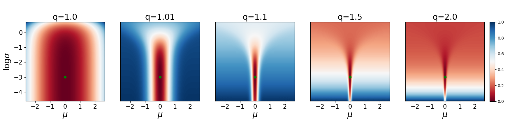
Figure 1: Bregman divergence $D_{\Omega}(\pi||\pi_{\!{}_{E}})$ associated with Tsallis entropy ($\Omega({\color[rgb]{0.0,0.0,0.0}p})=-\mathcal{T}_{q}^{1}({\color[rgb]{0.0,0.0,0.0}p})$) between two uni-variate Gaussian distributions $\pi=\mathcal{N}(\mu,\sigma^{2})$ and $\pi_{\!{}_{E}}=\mathcal{N}(0,(e^{-3})^{2})$ (green point in each subplot). In each subplot, we normalized the Bregman divergence so that the maximum value becomes 1. Note that for $q=1$, $D_{\Omega}(\pi||\pi_{\!{}_{E}})$ becomes the KL divergence $\mathrm{KL}(\pi||\pi_{\!{}_{E}})$.

For deeper understanding of Tsallis entropy and its associated Bregman divergence in regularized MDPs, we consider an example in Figure 1. We first assume that both learning agents’ and experts’ policies follow uni-variate Gaussian distributions $\pi=\mathcal{N}(\mu,\sigma^{2})$ and $\pi_{\!{}_{E}}=\mathcal{N}(0,(e^{-3})^{2})$, respectively. We then evaluate the Bregman divergence in Figure 1 by using its tractable form and varying $q$ from 1.0—which corresponds to the KL divergence—to 2.0. We observe that the constant $q$ from the Tsallis entropy affects the sensitivity of the associated Bregman divergence w.r.t. the mean and standard deviation of the learning agent’s policy $\pi$. Specifically, as $q$ increases, the size of the valley— relatively red regime in Figure 1—across the $\mu$-axis and $\log\sigma$-axis decreases. This suggests that for larger $q$, minimizing the Bregman divergence requires more tightly matching means and variances of $\pi$ and $\pi_{\!{}_{E}}$.

4 Algorithmic Consideration

1:  Input: A set $\mathcal{D}_{\!{}_{E}}$ of expert demonstration generated by expert policy $\pi_{\!{}_{E}}$, a reward approximator $r_{\theta}$, a policy $\pi_{\psi}$ for neural network parameters $\theta$ and $\psi$

2:  for each iteration do

3:     Sample rollout trajectories by using the learners policy $\pi_{\psi}$.

4:     Optimize $\theta$ with the discriminator $D_{r_{\theta},\pi_{\psi}}$ and the learning objective in Eq.(11).

5:     Optimize $\psi$ with Regularized Actor Critic by using $r_{\theta}$ as a reward function.

6:  end for

7:  Output: $\pi_{\psi}\approx\pi_{\!{}_{E}}$, $r_{\theta}(s,a)\approx t(s,a;\pi_{\!{}_{E}})$ (a solution of the IRL problem in Lemma 1).

Algorithm 1 Regularized Adversarial Inverse Reinforcement Learning (RAIRL)

Based on a solution for regularized IRL in the previous section, we focus on developing an IRL algorithm in this section. Particularly to recover the reward function $t(s,a;\pi_{\!{}_{E}})$ in Lemma 1, we design an adversarial training objective as follows. Motivated by AIRL (Fu et al., 2018), we consider the following structured discriminator associated with $\pi,r$ and $t$ in Lemma 1:

$$D_{r,\pi}(s,a)=\sigma(r(s,a)-t(s,a;\pi)),\sigma(z)=\frac{1}{1+e^{-z}},z\in\mathbb{R}.$$

Note that we can recover the discriminator of AIRL in Eq.(5) when $t(s,a)=\log\pi(a|s)$ ($\phi(x)=\log x$ and $\lambda=1$). Then, we consider the following optimization objective of the discriminator which is the same as that of AIRL:

$$\hat{t}(s,a;\pi):=\operatorname*{arg\,max}_{r\in\mathbb{R}^{\mathcal{S}\times\mathcal{A}}}~{}\mathbb{E}_{(s,a)\sim{d}_{\pi_{\!{}_{E}}}}\left[\log D_{r,\pi}(s,a)\right]+\mathbb{E}_{(s,a)\sim{d}_{\pi}}\left[\log(1-D_{r,\pi}(s,a))\right].$$ (11)

Since the function $x\mapsto a\log\sigma(x)+b\log(1-\sigma(x))$ attains its maximum at $\sigma(x)=\frac{a}{a+b}$, or equivalently at $x=\log\frac{a}{b}$  (Goodfellow et al., 2014; Mescheder et al., 2017), it can be shown that

$$\hat{t}(s,a;\pi)=t(s,a;\pi)+\log\frac{{d}_{\pi_{\!{}_{E}}}(s,a)}{{d}_{\pi}(s,a)}.$$ (12)

When $\pi=\pi_{\!{}_{E}}$ in Eq.(12), we have $\hat{t}(s,a;\pi_{\!{}_{E}})=t(s,a;\pi_{\!{}_{E}})$ since ${d}_{\pi}={d}_{\pi_{\!{}_{E}}}$, which means the maximizer $\hat{t}$ becomes the solution of IRL after the agent successfully imitates the expert policy $\pi_{\!{}_{E}}$. To do so, we consider the following iterative algorithm. Assuming that we find out the optimal reward approximator $\hat{t}(s,a;\pi^{(i)})$ in Eq.(12) for the policy $\pi^{(i)}$ of the $i$-th iteration, we get the policy $\pi^{(i+1)}$ by optimizing the following objective with gradient ascent:

$${\color[rgb]{0.0,0.0,0.0}\underset{\pi\in\Delta^{\mathcal{A}}_{\mathcal{S}}}{\mathrm{maximize}}~{}}\mathbb{E}_{(s,a)\sim d_{\pi}}\left[\hat{t}(s,a;\pi^{(i)})-\Omega(\pi(\cdot|s))\right].$$ (13)

The above expectation in Eq.(13) can be decomposed into the following two terms

$$\mathbb{E}_{(s,a)\sim d_{\pi}}\left[\hat{t}(s,a;\pi^{(i)})-\Omega(\pi(\cdot|s))\right] =\mathbb{E}_{(s,a)\sim d_{\pi}}\left[t(s,a;\pi^{(i)})-\Omega(\pi(\cdot|s))\right]-\mathrm{KL}(d_{\pi}||d_{\pi_{\!{}_{E}}})$$

$$=-\underbrace{\mathbb{E}_{(s,a)\sim d_{\pi}}\left[D_{\Omega}^{\mathcal{A}}(\pi(\cdot|s)||\pi^{(i)}(\cdot|s))\right]}_{\textrm{(I)}}-\underbrace{\mathrm{KL}(d_{\pi}||d_{\pi_{\!{}_{E}}})}_{\textrm{(II)}},$$ (14)

where the second equality follows since Lemma 1 tells us that $t(s,a;\pi^{(i)})$ is a reward function that makes $\pi^{(i)}$ an optimal policy in the $\Omega$-regularized MDP. Minimizing term (II) in Eq.(14) makes $\pi^{(i+1)}$ close to $\pi_{\!{}_{E}}$ while minimizing term (I) can be regarded as a conservative policy optimization around the policy $\pi^{(i)}$ (Schulman et al., 2015).

In practice, we parameterize our reward and policy approximations with neural networks and train them using an off-policy Regularized Actor-Critic (RAC) (Yang et al., 2019) as described in Algorithm 1.We evaluate our Regularized Adversarial Inverse Reinforcement Learning (RAIRL) approach across various scenarios, below.

5 Experiments

We summarize the experimental setup as follows. In our experiments, we consider $\Omega({\color[rgb]{0.0,0.0,0.0}p})=-\lambda\mathbb{E}_{a\sim{\color[rgb]{0.0,0.0,0.0}p}}[\phi({\color[rgb]{0.0,0.0,0.0}p}(a)]$ with the following regularizers from Yang et al. (2019): (1) Shannon entropy ($\phi(x)=-\log x$), (2) Tsallis entropy regularizer ($\phi(x)=\frac{k}{q-1}(1-x^{q-1})$), (3) $\mathrm{exp}$ regularizer ($\phi(x)=e-e^{x}$), (4) $\mathrm{cos}$ regularizer ($\phi(x)=\cos(\frac{\pi}{2}x)$), (5) $\mathrm{sin}$ regularizer ($\phi(x)=1-\sin\frac{\pi}{2}x$). The above regularizers were chosen since other regularizers have not been empirically validated to the best of our knowledge. We chose those regularizers to make our empirical analysis more tractable. In addition, we model the reward approximator of RAIRL as a neural network with either one of the following models: (1) Non-structured model (NSM)—a simple feed-forward neural network that outputs real values used in AIRL (Fu et al., 2018)—and (2) Density-based model (DBM)—a model using a neural network for $\pi$ (softmax for discrete controls and multi-variate Gaussian model for continuous controls) of the solution in Eq.(1) (See Appendix J.2 for detailed explanation). For RL algorithm of RAIRL, we implement Regularized Actor Critic (RAC) (Yang et al., 2019) on top of SAC implementation of Rlpyt (Stooke & Abbeel, 2019). Other settings are summarized in Appendix J. For all experiments, we use 5 runs and report 95% confidence interval.

5.1 Experiment 1: Multi-armed Bandit (Discrete Action)

We consider a 4-armed bandit environment as shown in Figure 2 (left). An expert policy $\pi_{\!{}_{E}}$ is assumed to be either dense (with probability 0.1, 0.2, 0.3, 0.4 for $a=0,1,2,3$) or sparse (with probability 0, 0, 1/3, 2/3 for $a=0,1,2,3$). For those experts, we use RAIRL with actions sampled from $\pi_{\!{}_{E}}$ and compare learned rewards with the ground truth reward $t(s,a;\pi_{\!{}_{E}})$ in Lemma 1. When $\pi_{\!{}_{E}}$ is dense, RAIRL successfully acquires the ground truth rewards irrespective of the reward model choices. When sparse $\pi_{\!{}_{E}}$ is used, however, RAIRL with a non-structured model (RAIRL-NSM) failed to recover the rewards for $a=0,1$—where $\pi_{\!{}_{E}}(a)=0$—due to the lack of samples at the end of the imitation. On the other hand, RAIRL with a density-based model (RAIRL-DBM) can recover the correct rewards due to the softmax layer which maintains the sum over the outputs equal to 1. Therefore, we argue that using DBM is necessary for correct reward acquisition since a set of demonstration is generally sparse. In the following experiment, we show the choice of reward models indeed affects the performance of rewards.

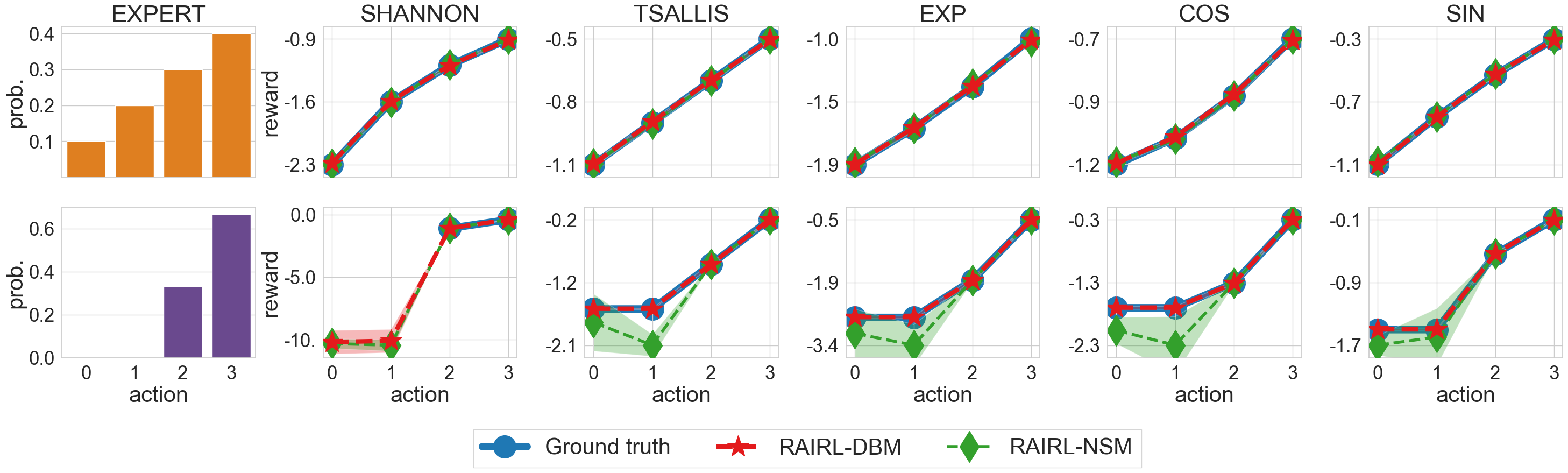
Figure 2: Expert policy (Left) and reward learned by RAIRL with different types of policy regularizers (Right) in Multi-armed Bandit. Either one of dense (Top row) or sparse (Bottom row) expert policies $\pi_{\!{}_{E}}$ is considered.

5.2 Experiment 2: Bermuda World (Continuous Observation, Discrete Action)

We consider an environment with a 2-dimensional continuous state space as described in Figure 3. At each episode, the learning agent is initialized uniformly on the $x$-axis between $-5$ and $5$, and there are 8 possible actions—an angle in $\{-\pi,-\frac{3}{4}\pi,...,\frac{1}{2}\pi,\frac{3}{4}\pi\}$ that determines the direction of movement. An expert in Bermuda World considers 3 target positions $(-5,10),(0,10),(5,10)$ and behaves stochastically. We state how we mathematically define the expert policy $\pi_{\!{}_{E}}$ in Appendix J.3. During RAIRL’s training (Figure 3, Top row), we use 1000 demonstrations sampled from the expert and periodically measure mean Bregman divergence, i.e., for $D_{\Omega}^{\mathcal{A}}(p_{1}||p_{2})=\mathbb{E}_{a\sim p_{1}}[f_{\phi}^{\prime}(p_{2}(a))-\phi(p_{1}(a))]-\mathbb{E}_{a\sim p_{2}}[f_{\phi}^{\prime}(p_{2}(a))-\phi(p_{2}(a))]$,

$$\frac{1}{N}\sum_{i=1}^{N}D_{\Omega}^{\mathcal{A}}(\pi(\cdot|s_{i})||\pi_{\!{}_{E}}(\cdot|s_{i})).$$

Here, the states $s_{1},...,s_{N}$ comes from 30 evaluation trajectories that are stochastically sampled from the agent’s policy $\pi$—which is fixed during evaluation—in a separate evaluation environment. During the evaluation of learned reward (Figure 3, Bottom row), we train randomly initialized agents with RAC and rewards acquired from RAIRL’s training and check if mean Bregman divergence is properly minimized. We measure mean Bregman divergence as was done in RAIRL’s training.

RAIRL-DBM is shown to minimize the target divergence more effectively compared to RAIRL-NSM during reward evaluation although both achieve comparable performances during RAIRL’s training. Moreover, we substitute $\lambda$ with $1,5,10$ and observe that learning with $\lambda$ larger than 1 returns better rewards—only $\lambda=1$ was considered in AIRL (Fu et al., 2018). Note that in all cases, the minimum divergence achieved by RAIRL is comparable with that of behavioral cloning (BC). This is because BC performs sufficiently well when many demonstration is given. We think the divergence of BC may be the near-optimal divergence that can be achieved with our policy neural network model.

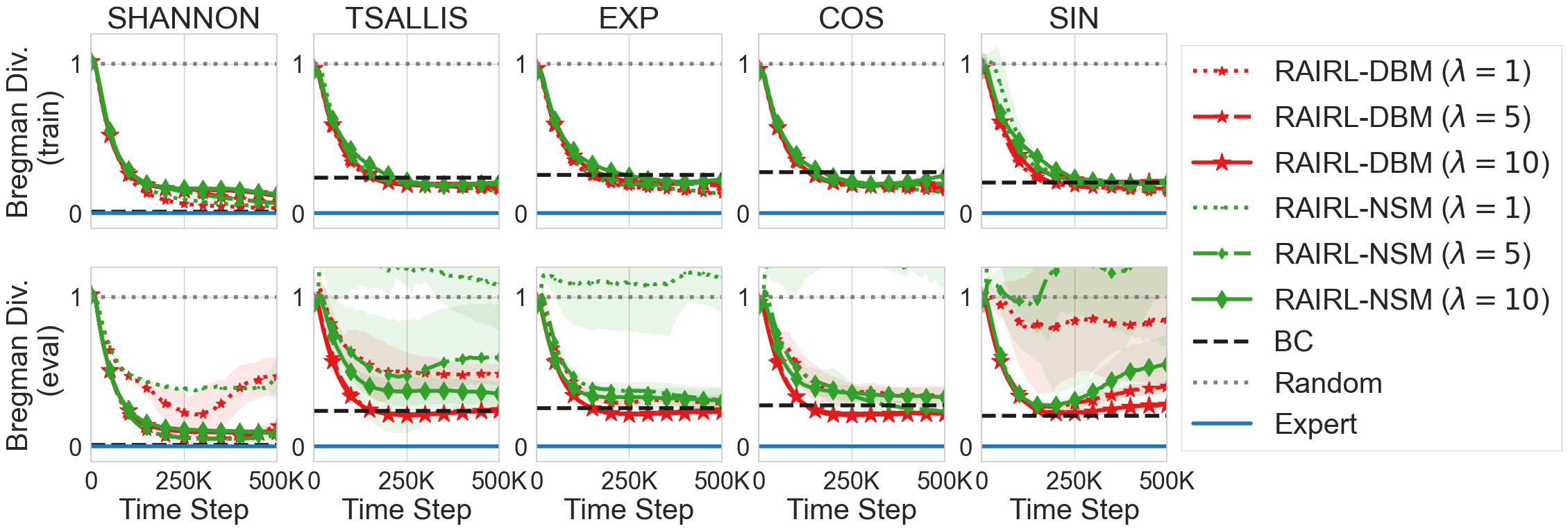
Figure 3: Mean Bregman divergence during training (Top row) and the divergence during reward evaluation (Bottom row) in Bermuda World. In each column, different policy regularizers and their respective target divergences are considered. The results are reported after normalization with the divergence of uniform random policy, and that of behavioral cloning (BC) is reported for comparison.

5.3 Experiment 3: MuJoCo (Continuous Observation and Action)

We validate RAIRL on MuJoCo continuous control tasks (Hopper-v2, Walker-v2, HalfCheetah-v2, Ant-v2) as follows. We assume multivariate-Gaussian policies (with diagonal covairance matrices) for both learner’s policy $\pi$ and expert policy $\pi_{\!{}_{E}}$. Instead of $\mathrm{tanh}$-squashed policy in Soft-Actor Critic (Haarnoja et al., 2018), we use hyperbolized environments—where $\mathrm{tanh}$ is regarded as a part of the environment—with additional engineering on the policy networks (See Appendix J.4 for details). We use 100 demonstrations stochastically sampled from $\pi_{\!{}_{E}}$ to validate RAIRL. In MuJoCo experiments, we focus on a set of Tsallis entropy regularizer ($\Omega=-\mathcal{T}_{q}^{1}$) with $q=1,1.5,2$—where Tsallis entropy becomes Shannon entropy for $q=1$. We then exploit the tractable quantities for multi-variate Gaussian distributions in Section 3.2 to stabilize RAIRL and check its performance in terms of mean Bregman divergence similar to the previous experiment. Note that since both $\pi$ and $\pi_{\!{}_{E}}$ are multi-variate Gaussian and can be evaluated, we can evaluate the individual Bregman divergence $D_{\Omega}^{\mathcal{A}}(\pi(\cdot|s)||\pi_{\!{}_{E}}(\cdot|s))$ on $s$ by using the derivation in Appendix I.3.

The performances during RAIRL’s training are described as follows. We report $\pi$ with both an episodic score (Figure 4) and mean Bregman divergences with respect to three types of Tsallis entropies (Figure 5) $\Omega=-\mathcal{T}_{q^{\prime}}^{1}$ with $q^{\prime}=1,1.5,2$. Note that the objective of RAIRL with $\Omega=-\mathcal{T}_{q}^{\color[rgb]{0.0,0.0,0.0}1}$ is to minimize the corresponding mean Bregman divergence with $q^{\prime}=q$. In Figure 4, both RAIRL-DBM and RAIRL-NSM are shown to achieve the expert performance, irrespective of $q$, in Hopper-v2, Walker-v2, and HalfCheetah-v2. In contrast, RAIRL in Ant-v2 fails to achieve the expert’s performance within 2,000,000 steps and RAIRL-NSM highly outperforms RAIRL-DBM in our setting. Although the episodic scores are comparable for all methods in Hopper-v2, Walker-v2, and HalfCheetah-v2, respective divergences are shown to be highly different from one another as shown in Figure 5. RAIRL with $q=2$ in most cases achieves the minimum mean Bregman divergence (for all three divergences with $q^{\prime}=1,1.5,2$), whereas RAIRL with $q=1$—which corresponds to AIRL (Fu et al., 2018)—achieves the maximum divergence in most cases. This result is in alignment with our intuition from Section 3.2; as $q$ increases, minimizing the Bregman divergence requires much tighter matching between $\pi$ and $\pi_{\!{}_{E}}$. Unfortunately, while evaluating the acquired reward—RAC with randomly initialized agent and acquired reward—the target divergence is not properly decreased in continuous controls. We believe this is because $\pi$ is a probability density function in continuous controls and causes large variance during training, while $\pi$ is a mass function and is well-bounded in discrete control problems.

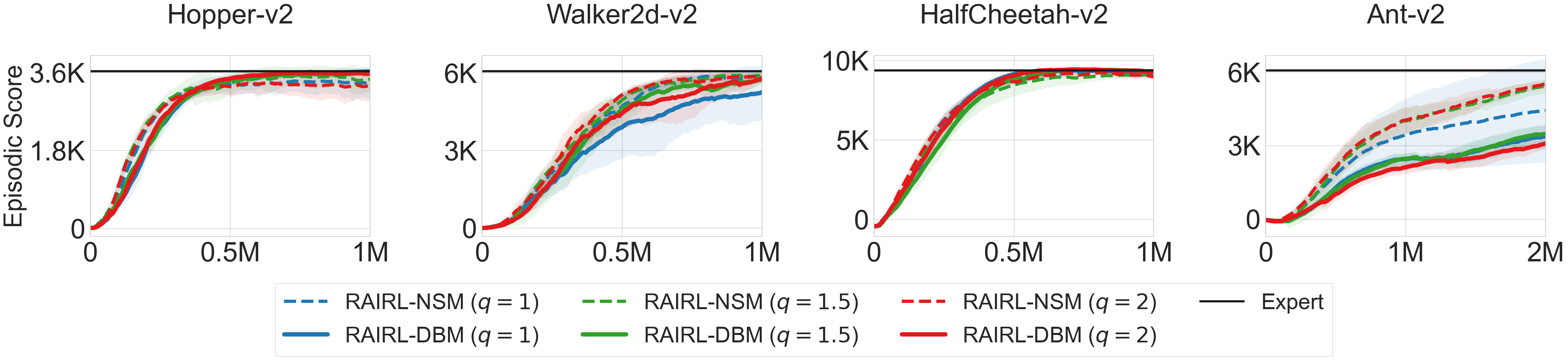
Figure 4: Averaged episodic score of RAIRL’s training in MuJoCo environments. RAIRL with $\mathcal{T}_{q}^{1}$ regularizer with $q=1,1.5,2$ is considered.

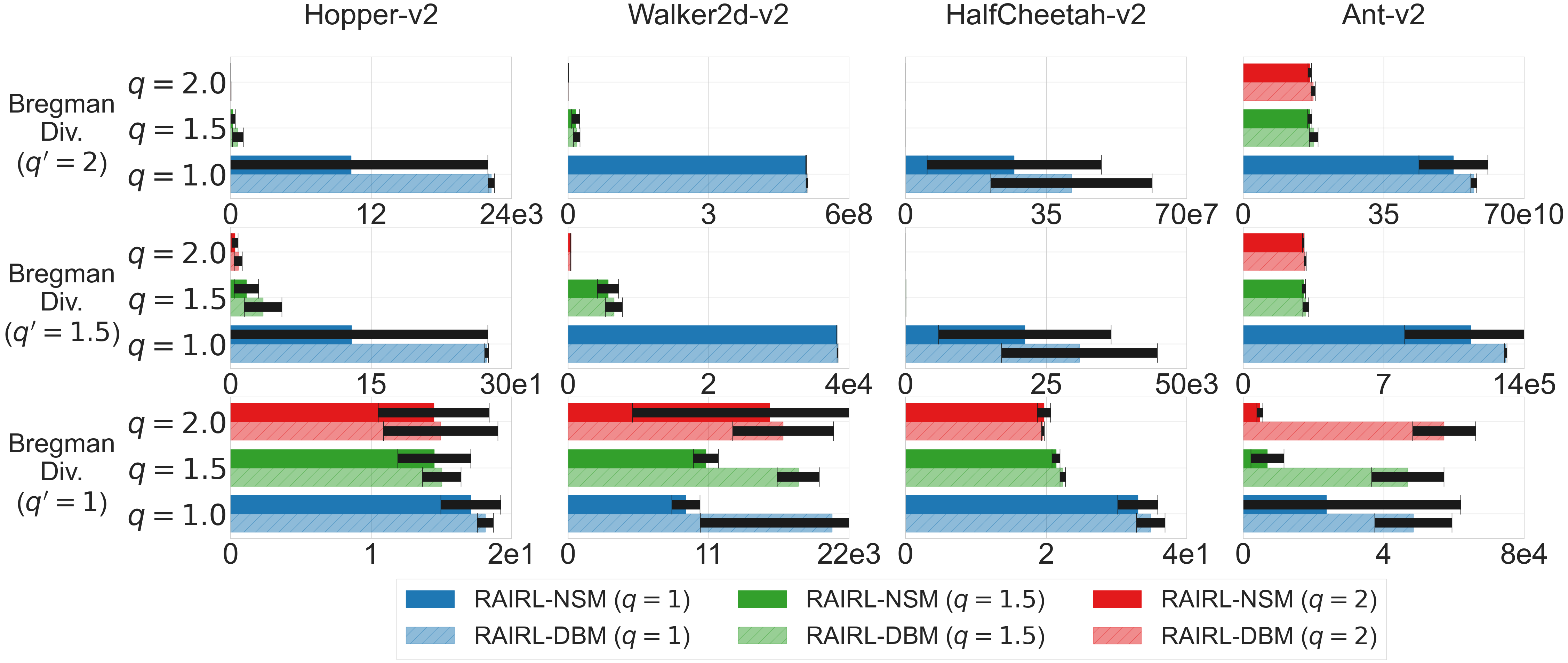
Figure 5: Bregman divergences with Tsallis entropy $\mathcal{T}_{q^{\prime}}^{1}$ with $q^{\prime}=1,1.5,2$ during RAIRL’s training in MuJoCo environments. We consider RAIRL with Tsallis entropy regularizer $\mathcal{T}_{q}^{1}$ with $q=1,1.5,2$.

6 Discussion and Future Works

We consider the problem of IRL in regularized MDPs (Geist et al., 2019), assuming a class of strongly convex policy regularizers. We theoretically derive its solution (a set of reward functions) and show that learning with these rewards is equivalent to a specific instance of imitation learning—i.e., one that minimizes the Bregman divergence associated with policy regularizers. We propose RAIRL—a practical sampled-based IRL algorithm in regularized MDPs—and evaluate its applicability on policy imitation (for discrete and continuous controls) and reward acquisition (for discrete control).

Finally, recent advances in imitation learning and IRL are built from the perspective of regarding imitation learning as statistical divergence minimization problems (Ke et al., 2019; Ghasemipour et al., 2019). Although Bregman divergence is known to cover various divergences, it does not include some divergence families such as $f$-divergence (Csiszár, 1963; Amari, 2009). Therefore, we believe that considering RL with policy regularization different from Geist et al. (2019) and its inverse problem is a possible way of finding the links between imitation learning and various statistical distances.

Appendix A Bellman Operators, Value Functions in regularized MDPs

Let a policy regularizer $\Omega:\Delta^{\mathcal{A}}\rightarrow\mathbb{R}$ be strongly convex, and define the convex conjugate of $\Omega$ is $\Omega^{*}:\mathbb{R}^{\mathcal{A}}\rightarrow\mathbb{R}$ as

$$\Omega^{*}(Q(s,\cdot)) =\max_{\pi(\cdot|s)\in\Delta^{\mathcal{A}}}\langle\pi(\cdot|s),Q(s,\cdot)\rangle_{\mathcal{A}}-\Omega(\pi(\cdot|s)),Q\in\mathbb{R}^{\mathcal{S}\times\mathcal{A}},s\in\mathcal{S}.$$ (15)

Then, Bellman operators, equations and value functions in regularied MDPs are defined as follows.

Definition 1 (Regularized Bellman Operators).

For $V\in\mathbb{R}^{\mathcal{S}}$, let us define $Q(s,a)=r(s,a)+\gamma\mathbb{E}_{s^{\prime}\sim P(\cdot|s,a)}[V(s^{\prime})]$. The regularized Bellman evaluation operator is defined as

$$[T^{\pi}V](s):=\langle\pi(\cdot|s),Q(s,\cdot)\rangle_{\mathcal{A}}-\Omega(\pi(\cdot|s)),s\in\mathcal{S},$$

and $T^{\pi}V=V$ is called the regularized Bellman equation. Also, the regularized Bellman optimality operator is defined as

$$[T^{*}V](s):=\max_{\pi(\cdot|s)\in\Delta^{\mathcal{A}}}[T^{\pi}V](s)=\Omega^{*}(Q(s,\cdot)),s\in\mathcal{S},$$

and $T^{*}V=V$ is called the regularized Bellman optimality equation.

Definition 2 (Regularized value functions).

The unique fixed point $V^{\pi}$ of the operator $T^{\pi}$ is called the state value function, and $Q^{\pi}(s,a)=r(s,a)+\gamma\mathbb{E}_{s^{\prime}\sim P(\cdot|s,a)}[V^{\pi}(s^{\prime})]$ is called the state-action value function. Also, the unique fixed point $V^{*}$ of the operator $T^{*}$ is called the optimal state value function, and $Q^{*}(s,a)=r(s,a)+\gamma\mathbb{E}_{s^{\prime}\sim P(\cdot|s,a)}[V^{*}(s^{\prime})]$ is called the optimal state-action value function.

It should be noted that Proposition 1 in Geist et al. (2019) tells us $\nabla\Omega^{*}(Q(s,\cdot))$ is a policy that uniquely maximizes Eq.(15). For example, when $\Omega(\pi(\cdot|s))=\sum_{a\sim\pi(\cdot|s)}\log\pi(a|s)$ (negative Shannon entropy), $\nabla\Omega^{*}(Q(s,\cdot))$ is a softmax policy, i.e., $\nabla\Omega^{*}(Q(s,\cdot))=\frac{\exp(Q(s,\cdot))}{\sum_{a^{\prime}\in\mathcal{A}}\exp(Q(s,a^{\prime}))}$. Due to this property, the optimal policy $\pi^{*}$ of a regularized MDP is uniquely found for the optimal state-action value function $Q^{*}$ which is also uniquely defined as the fixed point of $T^{*}$.

Appendix B Proof of Lemma 1

Let us define $\pi^{s}=\pi(\cdot|s)$. For $r(s,a)=t(s,a;\pi_{\!{}_{E}})$, the RL objective Eq.(1) satisfies

$$\mathbb{E}_{\pi}\left[\sum_{i=0}^{\infty}\gamma^{i}\left\{r(s_{i},a_{i})-\Omega(\pi^{s_{i}})\right\}\right]\overset{(\textrm{i})}{=}\mathbb{E}_{\pi}\left[\sum_{i=0}^{\infty}\gamma^{i}\left\{t(s,a;\pi_{\!{}_{E}})-\Omega(\pi^{s_{i}})\right\}\right]$$

$$\overset{(\textrm{ii})}{=}\mathbb{E}_{\pi}\left[\sum_{i=0}^{\infty}\gamma^{i}\left\{\Omega^{\prime}(s_{i},a_{i};\pi_{\!{}_{E}})-\mathbb{E}_{a\sim\pi_{\!{}_{E}}^{s_{i}}}\Omega^{\prime}(s_{i},a;\pi_{\!{}_{E}})+\Omega(\pi_{\!{}_{E}}^{s_{i}})-\Omega(\pi^{s_{i}})\right\}\right]$$

$$\overset{(\textrm{iii})}{=}\mathbb{E}_{\pi}\left[\sum_{i=0}^{\infty}\gamma^{i}\left\{\mathbb{E}_{a\sim\pi^{s_{i}}}\Omega^{\prime}(s_{i},a;\pi_{\!{}_{E}})-\mathbb{E}_{a\sim\pi_{\!{}_{E}}^{s_{i}}}\Omega^{\prime}(s_{i},a;\pi_{\!{}_{E}})+\Omega(\pi_{\!{}_{E}}^{s_{i}})-\Omega(\pi^{s_{i}})\right\}\right]$$

$$\overset{(\textrm{iv})}{=}\mathbb{E}_{\pi}\left[\sum_{i=0}^{\infty}\gamma^{i}\left\{\langle\nabla\Omega(\pi_{\!{}_{E}}^{s_{i}}),\pi^{s_{i}}\rangle_{\mathcal{A}}-\langle\nabla\Omega(\pi_{\!{}_{E}}^{s_{i}}),\pi_{\!{}_{E}}^{s_{i}}\rangle_{\mathcal{A}}+\Omega(\pi_{\!{}_{E}}^{s_{i}})-\Omega(\pi^{s_{i}})\right\}\right]$$

$$=\mathbb{E}_{\pi}\left[\sum_{i=0}^{\infty}\gamma^{i}\left\{\Omega(\pi_{\!{}_{E}}^{s_{i}})-\Omega(\pi^{s_{i}})+\langle\nabla\Omega(\pi_{\!{}_{E}}^{s_{i}}),\pi^{s_{i}}\rangle_{\mathcal{A}}-\langle\nabla\Omega(\pi_{\!{}_{E}}^{s_{i}}),\pi_{\!{}_{E}}^{s_{i}}\rangle_{\mathcal{A}}\right\}\right]$$

$$=-\mathbb{E}_{\pi}\left[\sum_{i=0}^{\infty}\gamma^{i}\left\{\Omega(\pi^{s_{i}})-\Omega(\pi_{\!{}_{E}}^{s_{i}})-\langle\nabla\Omega(\pi_{\!{}_{E}}^{s_{i}}),\pi^{s_{i}}\rangle_{\mathcal{A}}+\langle\nabla\Omega(\pi_{\!{}_{E}}^{s_{i}}),\pi_{\!{}_{E}}^{s_{i}}\rangle_{\mathcal{A}}\right\}\right]$$

$$=-\mathbb{E}_{\pi}\left[\sum_{i=0}^{\infty}\gamma^{i}\left\{\Omega(\pi^{s_{i}})-\Omega(\pi_{\!{}_{E}}^{s_{i}})-\langle\nabla\Omega(\pi_{\!{}_{E}}^{s_{i}}),\pi^{s_{i}}-\pi_{\!{}_{E}}^{s_{i}}\rangle_{\mathcal{A}}\right\}\right]\overset{(\textrm{v})}{=}-\mathbb{E}_{\pi}\left[\sum_{i=0}^{\infty}\gamma^{i}D_{\Omega}^{\mathcal{A}}(\pi^{s_{i}}||\pi_{\!{}_{E}}^{s_{i}}))\right],$$ (16)

where (i) follows from the assumption $r(s,a)=t(s,a;\pi_{\!{}_{E}})$ in Lemma 1, (ii) follows from the definition of $t(s,a;\pi)$ in Eq.(7), (iii) follows since taking the inner expectation first does not change the overall expectation, (iv) follows from the definition of $\Omega^{\prime}$ in Lemma 1 and $\sum_{a\in\mathcal{A}}{\color[rgb]{0.0,0.0,0.0}p}(a)[\nabla\Omega({\color[rgb]{0.0,0.0,0.0}p})](a)=\langle\nabla\Omega({\color[rgb]{0.0,0.0,0.0}p}),{\color[rgb]{0.0,0.0,0.0}p}\rangle_{\mathcal{A}}$, and (v) follows from the definition of Bregman divergence, i.e., $D_{\Omega}^{\mathcal{A}}({\color[rgb]{0.0,0.0,0.0}p_{1}}||{\color[rgb]{0.0,0.0,0.0}p_{2}})=\Omega({\color[rgb]{0.0,0.0,0.0}p_{1}})-\Omega({\color[rgb]{0.0,0.0,0.0}p_{2}})-\langle\nabla\Omega({\color[rgb]{0.0,0.0,0.0}p_{2}}),{\color[rgb]{0.0,0.0,0.0}p_{1}}-{\color[rgb]{0.0,0.0,0.0}p_{2}}\rangle_{\mathcal{A}}$. Due to the non-negativity of $D_{\Omega}^{\mathcal{A}}$, Eq.(16) is less than or equal to zero which can be achieved when $\pi=\pi_{\!{}_{E}}$.

Appendix C Proof of Corollary 1

Let $a\in\{1,...,|\mathcal{A}|\}$ and $\pi_{a}=\pi(a)$ for simplicity. For

$$\Omega(\pi)=-\lambda\mathbb{E}_{a\sim\pi}\phi(\pi_{a})=-\lambda\sum_{a\in\mathcal{A}}\pi_{a}\phi(\pi_{a})=-\lambda\sum_{a\in\mathcal{A}}f_{\phi}(\pi_{a})$$

with $f_{\phi}(x)=x\phi(x)$, we have

$$\nabla\Omega(\pi)=-\lambda\nabla_{\pi_{1},...,\pi_{|\mathcal{A}|}}{\sum_{a\in\mathcal{A}}f_{\phi}(\pi_{a})}=-\lambda[f_{\phi}^{\prime}(\pi_{1}),...,f_{\phi}^{\prime}(\pi_{|\mathcal{A}|})]^{T}$$

for $f_{\phi}^{\prime}(x)=\frac{\partial}{\partial x}(x\phi(x))$. Therefore, for $\pi^{s}=\pi(\cdot|s)$ we have

$$t(s,a;\pi) =[\nabla\Omega(\pi^{s})](a)-\langle\nabla\Omega(\pi^{s}),\pi^{s}\rangle_{\mathcal{A}}+\Omega(\pi^{s})$$

$$=-\lambda f_{\phi}^{\prime}(\pi^{s}_{a})-\left(\sum_{a^{\prime}\in\mathcal{A}}\pi^{s}_{a^{\prime}}(-\lambda f_{\phi}^{\prime}(\pi^{s}_{a^{\prime}}))\right)+\left(-\lambda\sum_{{a^{\prime}}\in\mathcal{A}}\pi^{s}_{a^{\prime}}\phi(\pi^{s}_{a^{\prime}})\right)$$

$$=-\lambda\left\{f_{\phi}^{\prime}(\pi^{s}_{a})-\left(\sum_{a^{\prime}\in\mathcal{A}}\pi^{s}_{a^{\prime}}f_{\phi}^{\prime}(\pi^{s}_{a^{\prime}})\right)+\left(\sum_{a^{\prime}\in\mathcal{A}}\pi^{s}_{a^{\prime}}\phi(\pi^{s}_{a^{\prime}})\right)\right\}$$

$$=-\lambda\left\{f_{\phi}^{\prime}(\pi^{s}_{a})-\sum_{a^{\prime}\in\mathcal{A}}\pi^{s}_{a^{\prime}}\left(f_{\phi}^{\prime}(\pi^{s}_{a^{\prime}})-\phi(\pi^{s}_{a^{\prime}})\right)\right\}$$

$$=-\lambda\left\{f_{\phi}^{\prime}(\pi^{s}_{a})-\mathbb{E}_{a^{\prime}\sim\pi^{s}}\left[f_{\phi}^{\prime}(\pi^{s}_{a^{\prime}})-\phi(\pi^{s}_{a^{\prime}})\right]\right\}.$$

Appendix D Proof of Optimal Rewards on Continuous Controls

Note that for two continuous distributions $\mathbb{P}_{1}$ and $\mathbb{P}_{2}$ having probability density functions $p_{1}(x)$ and $p_{2}(x)$, respectively, the Bregman divergence can be defined as (Guo et al., 2017; Jones & Byrne, 1990)

$$D_{\omega}^{\mathcal{X}}(\mathbb{P}_{1}||\mathbb{P}_{2}):=\int_{\mathcal{X}}\left\{\omega(p_{1}(x))-\omega(p_{2}(x))-\omega^{\prime}(p_{2}(x))(p_{1}(x)-p_{2}(x))\right\}dx,$$ (17)

where $\omega^{\prime}(x):=\frac{\partial}{\partial x}\omega(x)$ and the divergence is measure point-wisely on $x\in\mathcal{X}$. Let us assume

$$\Omega(\pi)=\int_{\mathcal{A}}\omega(\pi(a))da$$ (18)

for a probability density function $\pi$ on $\mathcal{A}$ and define

$$t(s,a;\pi):=\omega^{\prime}(\pi^{s}(a))-\int_{\mathcal{A}}\left[\pi^{s}(a^{\prime})\omega^{\prime}(\pi^{s}(a^{\prime}))-\omega(\pi^{s}(a^{\prime}))\right]da^{\prime}.$$ (19)

for $\pi^{s}=\pi(\cdot|s)$. For $r(s,a)=t(s,a;\pi_{\!{}_{E}})$, the RL objective in Eq.(1) satisfies

$$\mathbb{E}_{\pi}\left[\sum_{i=0}^{\infty}\gamma^{i}\left\{r(s_{i},a_{i})-\Omega(\pi^{s_{i}})\right\}\right]=\mathbb{E}_{\pi}\left[\sum_{i=0}^{\infty}\gamma^{i}\left\{t(s_{i},a_{i};\pi_{\!{}_{E}})-\Omega(\pi^{s_{i}})\right\}\right]$$

$$=\mathbb{E}_{\pi}\left[\sum_{i=0}^{\infty}\gamma^{i}\left\{\omega^{\prime}(\pi_{\!{}_{E}}^{s_{i}}(a_{i}))-\int_{\mathcal{A}}\left[\pi_{\!{}_{E}}^{s_{i}}(a)\omega^{\prime}(\pi_{\!{}_{E}}^{s_{i}}(a))-\omega(\pi_{\!{}_{E}}^{s_{i}}(a))\right]da-\int_{\mathcal{A}}\omega(\pi^{s_{i}}(a))da\right\}\right]$$

$$=\mathbb{E}_{\pi}\left[\sum_{i=0}^{\infty}\gamma^{i}\left\{\int_{\mathcal{A}}\pi^{s_{i}}(a)\omega^{\prime}(\pi_{\!{}_{E}}^{s_{i}}(a))da-\int_{\mathcal{A}}\left[\pi_{\!{}_{E}}^{s_{i}}(a)\omega^{\prime}(\pi_{\!{}_{E}}^{s_{i}}(a))-\omega(\pi_{\!{}_{E}}^{s_{i}}(a))+\omega(\pi^{s_{i}}(a))\right]da\right\}\right]$$

$$=\mathbb{E}_{\pi}\left[\sum_{i=0}^{\infty}\gamma^{i}\int_{\mathcal{A}}\left\{\pi^{s_{i}}(a)\omega^{\prime}(\pi_{\!{}_{E}}^{s_{i}}(a))-\left[\pi_{\!{}_{E}}^{s_{i}}(a)\omega^{\prime}(\pi_{\!{}_{E}}^{s_{i}}(a))-\omega(\pi_{\!{}_{E}}^{s_{i}}(a))+\omega(\pi^{s_{i}}(a))\right]\right\}da\right]$$

$$=\mathbb{E}_{\pi}\left[\sum_{i=0}^{\infty}\gamma^{i}\int_{\mathcal{A}}\left\{\omega(\pi_{\!{}_{E}}^{s_{i}}(a))-\omega(\pi^{s_{i}}(a))+\pi^{s_{i}}(a)\omega^{\prime}(\pi_{\!{}_{E}}^{s_{i}}(a))-\pi_{\!{}_{E}}^{s_{i}}(a)\omega^{\prime}(\pi_{\!{}_{E}}^{s_{i}}(a))\right\}da\right]$$

$$=-\mathbb{E}_{\pi}\left[\sum_{i=0}^{\infty}\gamma^{i}\int_{\mathcal{A}}\left\{\omega(\pi^{s_{i}}(a))-\omega(\pi_{\!{}_{E}}^{s_{i}}(a))-\pi^{s_{i}}(a)\omega^{\prime}(\pi_{\!{}_{E}}^{s_{i}}(a))+\pi_{\!{}_{E}}^{s_{i}}(a)\omega^{\prime}(\pi_{\!{}_{E}}^{s_{i}}(a))\right\}da\right]$$

$$=-\mathbb{E}_{\pi}\left[\sum_{i=0}^{\infty}\gamma^{i}\int_{\mathcal{A}}\left\{\omega(\pi^{s_{i}}(a))-\omega(\pi_{\!{}_{E}}^{s_{i}}(a))-\omega^{\prime}(\pi_{\!{}_{E}}^{s_{i}}(a))\left(\pi^{s_{i}}(a)-\pi_{\!{}_{E}}^{s_{i}}(a)\right)\right\}da\right]$$

$$=-\mathbb{E}_{\pi}\left[\sum_{i=0}^{\infty}\gamma^{i}D_{\omega}^{\mathcal{A}}(\pi^{s_{i}}||\pi_{\!{}_{E}}^{s_{i}}))\right],$$ (20)

where (i) follows from $r(s,a)=t(s,a;\pi_{\!{}_{E}})$, (ii) follows from Eq.(18) and Eq.(19), and (iii) follows from the definition of Bregman divergence in Eq.(17). Due to the non-negativity of $D_{\omega}$, Eq.(24) is less than or equal to zero which can be achieved when $\pi=\pi_{\!{}_{E}}$. Also, $\pi=\pi_{\!{}_{E}}$ is a unique solution since Eq.(1) has a unique solution for arbitrary reward functions.

Appendix E Proof of Lemma 2

Since Lemma 2 was mentioned but not proved in Geist et al. (2019), we remain the rigorous proof for Lemma 2 in this subsection. Note that we follow the proof idea in Ng et al. (1999).

First, let us assume an MDP $\mathcal{M}^{r}$ with a reward $r$ and corresponding optimal policy $\pi^{*}$. From Definition 1, the optimal state-value function $V^{*,r}$ and its corresponding state-action value function $Q^{*,r}(s,a):=r(s,a)+\gamma\mathbb{E}_{s^{\prime}\sim P(\cdot|s,a)}[V^{*,r}(s^{\prime})]$ should satisfies the regularized Bellman optimality equation

$$V^{*,r}(s) =T^{*,r}V^{*,r}(s)=\Omega^{*}(Q^{*,r}(s,a))$$

$$=\max_{\pi(\cdot|s)\in\Delta^{\mathcal{A}}}\langle\pi(\cdot|s),Q^{*,r}(s,a)\rangle_{\mathcal{A}}-\Omega(\pi(\cdot|s))$$

$$=\max_{\pi(\cdot|s)\in\Delta^{\mathcal{A}}}\langle\pi(\cdot|s),r(s,a)+\gamma\mathbb{E}_{s^{\prime}\sim P(\cdot|s,a)}[V^{*,r}(s^{\prime})]\rangle_{\mathcal{A}}-\Omega(\pi(\cdot|s)),$$ (21)

where we explicitize the dependencies on $r$. Also, the optimal policy $\pi^{*}$ is a unique maximizer for the above maximization.

Now, let us consider the shaped rewards $r(s,a)+\Phi(s^{\prime})-\Phi(s)$ and $r(s,a)+\mathbb{E}_{s^{\prime}\sim P(\cdot|s,a)}\Phi(s^{\prime})-\Phi(s)$. Please note that for both rewards, the expectation over $s^{\prime}$ for given $s,a$ is equal to

$$\tilde{r}(s,a)=r(s,a)+\mathbb{E}_{s^{\prime}\sim P(\cdot|s,a)}\Phi(s^{\prime})-\Phi(s),$$

and thus, it is sufficient to only consider the optimality for $\tilde{r}$. By subtracting $\Phi(s)$ from the regularized optimality Bellman equation for $r$ in Eq.(21), we have

$$V^{*,r}(s)-\Phi(s)$$

$$=\max_{\pi(\cdot|s)\in\Delta^{\mathcal{A}}}\langle\pi(\cdot|s),r(s,a)+\gamma\mathbb{E}_{s^{\prime}\sim P(\cdot|s,a)}\Phi(s^{\prime})-\Phi(s)+\gamma\mathbb{E}_{s^{\prime}\sim P(\cdot|s,a)}[V^{*,r}(s^{\prime})-\Phi(s^{\prime})]\rangle_{\mathcal{A}}$$

$$~{}~{}~{}~{}~{}~{}~{}~{}~{}~{}~{}~{}~{}~{}~{}~{}~{}~{}~{}~{}-\Omega(\pi(\cdot|s))$$

$$=\max_{\pi(\cdot|s)\in\Delta^{\mathcal{A}}}\langle\pi(\cdot|s),\tilde{r}(s,a)+\gamma\mathbb{E}_{s^{\prime}\sim P(\cdot|s,a)}[V^{*,r}(s^{\prime})-\Phi(s^{\prime})]\rangle_{\mathcal{A}}-\Omega(\pi(\cdot|s))$$

$$=[T^{*,\tilde{r}}(V^{*,r}-\Phi)](s).$$

That is, $V^{*,r}-\Phi$ is the fixed point of the regularized Bellman optimality operator $T^{*,\tilde{r}}$ associated with the shaped reward $\tilde{r}$. Also, a maximizer for the above maximization is $\pi^{*}$ since subtracting $\Phi(s)$ from Eq.(21) does not change the unique maximizer $\pi^{*}$.

Appendix F Comparison between our solution and existing solution in Geist et al. (2019)

F.1 Problems of Existing Solutions in Geist et al. (2019)

In Proposition 5 of Geist et al. (2019), a solution of regularized IRL is given, and we rewrite the relevant theorem in this subsection. Let us consider a regularized IRL problem, where $\pi_{\!{}_{E}}\in\Delta_{\mathcal{S}}^{\mathcal{A}}$ is an expert policy. Assuming that both the model (dynamics, discount factor and regularizer) and the expert policy are known, Geist et al. (2019) proposed a solution of regularized IRL as follows:

Lemma 4 (A solution of regularized IRL from Geist et al. (2019)).

Let $Q_{\!{}_{E}}\in\mathbb{R}^{\mathcal{S}\times\mathcal{A}}$ be a function such that $\pi_{E}(\cdot|s)=\nabla\Omega^{*}(Q_{\!{}_{E}}(s,\cdot)),s\in\mathcal{S}$. Also, define

$$r_{\!{}_{E}}(s,a) :=Q_{\!{}_{E}}(s,a)-\gamma\mathbb{E}_{s^{\prime}\sim P(\cdot|s,a)}[\Omega^{*}(Q_{\!{}_{E}}(s^{\prime},\cdot))]$$

$$=Q_{\!{}_{E}}(s,a)-\gamma\mathbb{E}_{s^{\prime}\sim P(\cdot|s,a)}[\langle\pi_{\!{}_{E}}(\cdot|s^{\prime}),Q_{\!{}_{E}}(s^{\prime},\cdot)\rangle_{\mathcal{A}}-\Omega(\pi_{\!{}_{E}}(\cdot|s^{\prime}))].$$

Then in the $\Omega$-regularized MDP with the reward $r_{\!{}_{E}}$, $\pi_{\!{}_{E}}$ is an optimal policy.

Proof.

Although the brief idea of the proof is given in Geist et al. (2019), we rewrite the proof in a more rigorous way as follows. Let us define $V_{\!{}_{E}}(s)=\langle\pi_{\!{}_{E}}(\cdot|s),Q_{\!{}_{E}}(s,\cdot)\rangle_{\mathcal{A}}-\Omega(\pi_{\!{}_{E}}(\cdot|s))$. Then, $r_{\!{}_{E}}(s,a)=Q_{\!{}_{E}}(s,a)-\gamma\mathbb{E}_{s^{\prime}\sim P(\cdot|s,a)}[V_{\!{}_{E}}(s^{\prime})]$, and thus, $Q_{\!{}_{E}}(s,a)=r_{\!{}_{E}}(s,a)+\gamma\mathbb{E}_{s^{\prime}\sim P(\cdot|s,a)}[V_{\!{}_{E}}(s^{\prime})]$. By using this and regularized Bellman optimality operator, we have

$$[T^{*}V_{\!{}_{E}}](s) \overset{(\textrm{i})}{=}\Omega^{*}(Q_{\!{}_{E}}(s,\cdot))\overset{(\textrm{ii})}{=}\max_{\pi(\cdot|s)\in\Delta^{\mathcal{A}}}\langle\pi(\cdot|s),Q_{\!{}_{E}}(s,\cdot)\rangle_{\mathcal{A}}-\Omega(\pi(\cdot|s))$$

$$\overset{(\textrm{iii})}{=}\langle\pi_{\!{}_{E}}(\cdot|s),Q_{\!{}_{E}}(s,\cdot)\rangle_{\mathcal{A}}-\Omega(\pi_{\!{}_{E}}(\cdot|s))=V_{\!{}_{E}}(s),$$

where (i) and (ii) follow from Definition 1, and (iii) follows since $\pi_{\!{}_{E}}$ is a unique maximizer. Thus, $V_{\!{}_{E}}$ is the fixed point of $T^{*}$, and $\pi_{E}(\cdot|s)=\nabla\Omega^{*}(Q_{\!{}_{E}}(s,\cdot)),s\in\mathcal{S},$ becomes an optimal policy. ∎

For example, when negative Shannon entropy is used as a regularizer, we can get $r_{\!{}_{E}}(s,a)=\log\pi_{\!{}_{E}}(a|s)$ by setting $Q_{\!{}_{E}}(s,a)=\log\pi_{\!{}_{E}}(a|s)$. However, a solution proposed in Lemma 4 has two crucial issues:
Issue 1. It requires the knowledge on the model dynamics, which is generally intractable.
Issue 2. We need to figure out $Q_{\!{}_{E}}$ that satisfies $\pi_{\!{}_{E}}(\cdot|s)=\nabla\Omega^{*}(Q_{\!{}_{E}}(s,\cdot))$, which comes from the relationship between optimal value function and optimal policy (Geist et al., 2019).

In the following subsection, we show how our solution in Lemma 1 is related to the solution from Geist et al. (2019) in Lemma 4.

F.2 From the solution of Geist et al. (2019) to the tractable solution

Let us consider the expert policy $\pi_{\!{}_{E}}$ and quantities $Q_{\!{}_{E}}$ and $r_{\!{}_{E}}$ satisfying the conditions in Lemma 4. From Lemma 2, a regularized MDP with the shaped reward

$$\tilde{r}_{\!{}_{E}}(s,a):=r_{\!{}_{E}}(s,a)+\gamma\mathbb{E}_{s^{\prime}\sim P(\cdot|s,a)}\Phi(s^{\prime})-\Phi(s)$$

for $\Phi\in\mathbb{R}^{\mathcal{S}}$ has its optimal policy as $\pi_{\!{}_{E}}$. Since $\Phi$ can be arbitrarily chosen, let us assume $\Phi(s)=\Omega^{*}(Q_{\!{}_{E}}(s,\cdot))$. Then, we have

$$\tilde{r}_{\!{}_{E}}(s,a) =r_{\!{}_{E}}(s,a)+\gamma\mathbb{E}_{s^{\prime}\sim P(\cdot|s,a)}\Phi(s^{\prime})-\Phi(s)$$

$$=\left\{Q_{\!{}_{E}}(s,a)-\gamma\mathbb{E}_{s^{\prime}\sim P(\cdot|s,a)}[\Omega^{*}(Q_{\!{}_{E}}(s^{\prime},\cdot))]\right\}+\mathbb{E}_{s^{\prime}\sim P(\cdot|s,a)}\Omega^{*}(Q_{\!{}_{E}}(s^{\prime},\cdot))-\Omega^{*}(Q_{\!{}_{E}}(s,\cdot))$$

$$=Q_{\!{}_{E}}(s,a)-\Omega^{*}(Q_{\!{}_{E}}(s,\cdot)).$$ (22)

Note that the reward in $Eq.(\ref{eq:newsolution1})$ does not require the knowledge on the model dynamics, which addresses Issue 1 in Appendix F.1. Also, by using $V_{\!{}_{E}}(s)=\Omega^{*}(Q_{\!{}_{E}}(s,\cdot))$ in the proof of Lemma 4, the reward in $Eq.(\ref{eq:newsolution1})$ can be written as

$$\tilde{r}_{\!{}_{E}}(s,a)=Q_{\!{}_{E}}(s,a)-V_{\!{}_{E}}(s),$$

which means $\tilde{r}_{\!{}_{E}}(s,a)$ is an advantage function for the optimal policy $\pi_{\!{}_{E}}$ in the $\Omega$-regularized MDP.

However, we still have Issue 2 in Appendix F.1 since $\Omega^{*}$ in $Eq.(\ref{eq:newsolution1})$ is generally intractable (Geist et al., 2019), which prevents us to find out appropriate $Q_{\!{}_{E}}(s,a)$. Interestingly, we show that for all $s\in S$ and $Q_{\!{}_{E}}(s,\cdot)=\nabla\Omega(\pi_{\!{}_{E}}(\cdot|s))$,

$$\nabla\Omega^{*}(Q_{\!{}_{E}}(s,\cdot)) =\operatorname*{arg\,max}_{\pi(\cdot|s)\in\Delta^{\mathcal{A}}}\langle\pi(\cdot|s),Q_{\!{}_{E}}(s,\cdot)\rangle_{\mathcal{A}}-\Omega(\pi(\cdot|s))$$

$$=\operatorname*{arg\,max}_{\pi(\cdot|s)\in\Delta^{\mathcal{A}}}\langle\pi(\cdot|s),\nabla\Omega(\pi_{\!{}_{E}}(\cdot|s))\rangle_{\mathcal{A}}-\Omega(\pi(\cdot|s))$$

$$=\operatorname*{arg\,min}_{\pi(\cdot|s)\in\Delta^{\mathcal{A}}}\Omega(\pi(\cdot|s))-\langle\nabla\Omega(\pi_{\!{}_{E}}(\cdot|s)),\pi(\cdot|s)\rangle_{\mathcal{A}}$$

$$=\operatorname*{arg\,min}_{\pi(\cdot|s)\in\Delta^{\mathcal{A}}}\Omega(\pi(\cdot|s))-\Omega(\pi_{\!{}_{E}}(\cdot|s))-\langle\nabla\Omega(\pi_{\!{}_{E}}(\cdot|s)),\pi(\cdot|s)-\pi_{\!{}_{E}}(\cdot|s)\rangle_{\mathcal{A}}$$

$$=\operatorname*{arg\,min}_{\pi(\cdot|s)\in\Delta^{\mathcal{A}}}D_{\Omega}^{\mathcal{A}}(\pi(\cdot|s)||\pi_{\!{}_{E}}(\cdot|s))=\pi_{\!{}_{E}}(\cdot|s),$$

where the last equality holds since the Bregman divergence $D_{\Omega}^{\mathcal{A}}(\pi(\cdot|s)||\pi_{\!{}_{E}}(\cdot|s))$ is greater than or equal to zero and its lowest value is achieved when $\pi(\cdot|s)=\pi_{\!{}_{E}}(\cdot|s)$. This means that when $Q_{\!{}_{E}}(s,\cdot)=\nabla\Omega(\pi_{\!{}_{E}}(\cdot|s))$ is used, the condition $\pi_{\!{}_{E}}(\cdot|s)=\nabla\Omega^{*}(Q_{\!{}_{E}}(s,\cdot))$ in Lemma 4 is satisfied without knowing the tractable form of $\Omega^{*}$ or $\nabla\Omega^{*}$, and thus, Issue 2 in Appendix F.1 is addressed—while we require the knowledge on the gradient $\nabla\Omega$ of the policy regularizer $\Omega$, which is practically more tractable. Finally, by substituting $Q_{\!{}_{E}}(s,\cdot)=\Omega^{\prime}(s,\cdot;\pi_{\!{}_{E}})$ for $\Omega^{\prime}(s,\cdot;\pi):=\nabla\Omega(\pi(\cdot|s)),s\in\mathcal{S},$ to Eq.(22), we have

$$\tilde{r}_{\!{}_{E}}(s,a) =\Omega^{\prime}(s,a;\pi_{\!{}_{E}})-\Omega^{*}(\Omega^{\prime}(s,\cdot;\pi_{\!{}_{E}}))$$

$$=\Omega^{\prime}(s,a;\pi_{\!{}_{E}})-\left\{\langle\pi_{\!{}_{E}}(\cdot|s),\Omega^{\prime}(s,\cdot;\pi_{\!{}_{E}})\rangle_{\mathcal{A}}-\Omega(\pi_{\!{}_{E}}(\cdot|s))\right\}$$

$$=\Omega^{\prime}(s,a;\pi_{\!{}_{E}})-\mathbb{E}_{a^{\prime}\sim\pi_{\!{}_{E}}(\cdot|s)}[\Omega^{\prime}(s,a^{\prime};\pi_{\!{}_{E}})]+\Omega(\pi_{\!{}_{E}}(\cdot|s))$$

$$=t(s,a;\pi_{\!{}_{E}}),$$

where $t(s,a;\pi_{\!{}_{E}})$ is our proposed solution in Lemma 1.

Appendix G Proof of Lemma 3

RL objective in Regularized MDPs w.r.t. normalized visitation distributions.

For a reward function $r\in\mathbb{R}^{{\mathcal{S}\times\mathcal{A}}}$ and a strongly convex function $\Omega:\Delta^{\mathcal{A}}\rightarrow\mathbb{R}$, the RL objetive $J_{\Omega}(r,\pi)$ in Eq.(1) is equivalent to

$$\operatorname*{arg\,max}_{\pi}\bar{J}_{\bar{\Omega}}(r,d_{\pi}):=\langle r,d_{\pi}\rangle_{{\mathcal{S}\times\mathcal{A}}}-\bar{\Omega}(d_{\pi}),$$ (23)

where for a set $\mathcal{D}$ of normalized visitation distributions (Syed et al., 2008)

$$\mathcal{D}:=\left\{d\in\Delta^{\mathcal{S}\times\mathcal{A}}:\sum_{a^{\prime}}d(s^{\prime},a^{\prime})=(1-\gamma)P_{0}(s^{\prime})+\gamma\sum_{s,a}P(s^{\prime}|s,a)d(s,a),\forall s^{\prime}\in\mathcal{S}\right\},$$

we define $\bar{\Omega}({d}):=\mathbb{E}_{(s,a)\sim d}[\Omega(\bar{\pi}_{d}(\cdot|s))]$ and $\bar{\pi}_{d}(\cdot|s):=\frac{{d}(s,\cdot)}{\sum_{a^{\prime}}{d}(s,a^{\prime})}\in\Delta_{\mathcal{S}}^{\mathcal{A}}$ for $d\in\mathcal{D}$ and use $\bar{\pi}_{d_{\pi}}(\cdot|s)=\pi(\cdot|s)$ for all $s\in\mathcal{S}$. For $\bar{\Omega}:\mathcal{D}\rightarrow\mathbb{R}$, its convex conjugate $\bar{\Omega}^{*}$ is

$$\bar{\Omega}^{*}(r): =\max_{d\in\mathcal{D}}\bar{J}_{\bar{\Omega}}(r,d)$$

$$=\max_{d\in\mathcal{D}}\langle r,d\rangle_{{\mathcal{S}\times\mathcal{A}}}-\bar{\Omega}(d)$$

$$\overset{(\mathrm{i})}{=}\max_{\pi\in\Delta_{\mathcal{S}}^{\mathcal{A}}}\langle r,d_{\pi}\rangle_{{\mathcal{S}\times\mathcal{A}}}-\bar{\Omega}(d_{\pi})$$

$$=\max_{\pi\in\Delta_{\mathcal{S}}^{\mathcal{A}}}\sum_{s,a}d_{\pi}(s,a)\left[r(s,a)-\Omega(\pi(a|s))\right]$$

$$=(1-\gamma)\cdot\max_{\pi\in\Delta_{\mathcal{S}}^{\mathcal{A}}}J_{\Omega}(r,\pi),$$ (24)

where $(\mathrm{i})$ follows from using the one-to-one correspondence between policies and visitation distributions (Syed et al., 2008; Ho & Ermon, 2016). Note that Eq.(24) is equal to the optimal discounted average return in regularized MDPs.

IRL objective in Regularized MDPs w.r.t. normalized visitation distributions.

By using the RL objective in Eq.(23), we can rewrite the IRL objective in Eq.(6) w.r.t. the normalized visitation distributions as the maximization of the following objective over $r\in\mathbb{R}^{\mathcal{S}\times\mathcal{A}}$:

$$(1-\gamma)\cdot\left\{J_{\Omega}(r,\pi_{\!{}_{E}})-\max_{\pi\in\Delta_{\mathcal{S}}^{\mathcal{A}}}J_{\Omega}(r,\pi)\right\}$$

$$=\bar{J}_{\bar{\Omega}}(r,d_{\pi_{\!{}_{E}}})-\max_{d\in\mathcal{D}}\bar{J}_{\bar{\Omega}}(r,d)$$

$$=\min_{d\in\mathcal{D}}\left\{\bar{J}_{\bar{\Omega}}(r,d_{\pi_{\!{}_{E}}})-\bar{J}_{\bar{\Omega}}(r,d)\right\}$$

$$=\min_{d\in\mathcal{D}}\left\{\left(\langle r,d_{\pi_{\!{}_{E}}}\rangle_{{\mathcal{S}\times\mathcal{A}}}-\bar{\Omega}(d_{\pi_{\!{}_{E}}})\right)-\left(\langle r,d\rangle_{{\mathcal{S}\times\mathcal{A}}}-\bar{\Omega}(d)\right)\right\}$$

$$=\min_{d\in\mathcal{D}}\left\{\bar{\Omega}(d)-\bar{\Omega}(d_{\pi_{\!{}_{E}}})-\langle r,d-d_{\pi_{\!{}_{E}}}\rangle_{{\mathcal{S}\times\mathcal{A}}}\right\}.$$ (25)

Note that if $\nabla\bar{\Omega}(d)$ is well-defined and $r=\nabla\bar{\Omega}(d_{\pi_{\!{}_{E}}})$ for any strictly convex $\bar{\Omega}$, Eq.(25) is equal to

$$\min_{d\in\mathcal{D}}\left\{\bar{\Omega}(d)-\bar{\Omega}(d_{\pi_{\!{}_{E}}})-\langle\nabla\bar{\Omega}(d_{\pi_{\!{}_{E}}}),d-d_{\pi_{\!{}_{E}}}\rangle_{{\mathcal{S}\times\mathcal{A}}}\right\}=\min_{d\in\mathcal{D}}D_{\bar{\Omega}}^{\mathcal{S}\times\mathcal{A}}(d||d_{\pi_{\!{}_{E}}}),$$

where the equality comes from the definition of Bregman divergence.

Proof of $t(s,a;\pi_{d})=\nabla[\bar{\Omega}(d)](s,a)$.

For simpler notation, we use matrix-vector notation for the proof when discrete state and action spaces $\mathcal{S}=\{1,...,|\mathcal{S}|\}$ and $\mathcal{A}=\{1,...,|\mathcal{A}|\}$ are considered. For a normalized visitation distribution $d\in\mathcal{D}$, let us define

$$d^{s}_{a} :=d(s,a),s\in\mathcal{S},a\in\mathcal{A},$$

$$\boldsymbol{d}^{s} :=[d^{s}_{1},...,d^{s}_{|\mathcal{A}|}]^{T}\in\mathbb{R}^{\mathcal{A}},s\in\mathcal{S},$$

$$\boldsymbol{D} :=[\boldsymbol{d}^{1},...,\boldsymbol{d}^{|\mathcal{S}|}]^{T}=\begin{bmatrix}d^{1}_{1}&\cdots&d^{1}_{|\mathcal{A}|}\\ \vdots&\ddots&\vdots\\ d^{|\mathcal{S}|}_{1}&\cdots&d^{|\mathcal{S}|}_{|\mathcal{A}|}\\ \end{bmatrix}\in\mathbb{R}^{\mathcal{S}\times\mathcal{A}},$$

$$\bar{\boldsymbol{\pi}}(\boldsymbol{x}) :=\frac{\boldsymbol{x}}{\boldsymbol{\mathit{1}}_{\mathcal{A}}^{T}\boldsymbol{x}}=\frac{1}{\sum_{a\in\mathcal{A}}x_{a}}\left[x_{1},...,x_{|\mathcal{A}|}\right]^{T}\in\mathbb{R}^{\mathcal{A}},\boldsymbol{x}:=\left[x_{1},...,x_{|\mathcal{A}|}\right]^{T}\in\mathbb{R}^{\mathcal{A}},$$

where $\boldsymbol{\mathit{1}}_{\mathcal{A}}=[1,...,1]^{T}\in\mathbb{R}^{\mathcal{A}}$ is an $|\mathcal{A}|$-dimensional all-one vector. By using these notations, the original $\bar{\Omega}$ can be rewritten as

$$\bar{\Omega}(\boldsymbol{D})=\sum_{s,a}d^{s}_{a}\Omega(\bar{\boldsymbol{\pi}}(\boldsymbol{d}^{s}))=\sum_{s\in\mathcal{S}}\boldsymbol{\mathit{1}}_{\mathcal{A}}^{T}\boldsymbol{d}^{s}\Omega(\bar{\boldsymbol{\pi}}(\boldsymbol{d}^{s})).$$

The gradient of $\bar{\Omega}$ w.r.t. $\boldsymbol{D}$ (using denominator-layout notation) is

$$\nabla_{\boldsymbol{D}}\bar{\Omega}(\boldsymbol{D}) =\left[\dfrac{\partial\bar{\Omega}(\boldsymbol{D})}{\partial\boldsymbol{d}^{1}},...,\dfrac{\partial\bar{\Omega}(\boldsymbol{D})}{\partial\boldsymbol{d}^{|\mathcal{S}|}}\right]^{T}\in\mathbb{R}^{\mathcal{S}\times\mathcal{A}},$$

where each element of $\nabla_{\boldsymbol{D}}\bar{\Omega}(\boldsymbol{D})$ satisfies

$$\dfrac{\partial\bar{\Omega}(\boldsymbol{D})}{\partial\boldsymbol{d}^{s}} =\left[\dfrac{\partial\bar{\Omega}(\boldsymbol{D})}{\partial d^{s}_{1}},...,\dfrac{\partial\bar{\Omega}(\boldsymbol{D})}{\partial d^{s}_{|\mathcal{A}|}}\right]^{T}$$

$$=\frac{\partial}{\partial\boldsymbol{d}^{s}}\left\{\sum_{s\in\mathcal{S}}\boldsymbol{\mathit{1}}_{\mathcal{A}}^{T}\boldsymbol{d}^{s}\Omega(\bar{\boldsymbol{\pi}}(\boldsymbol{d}^{s}))\right\}$$

$$=\Omega(\bar{\boldsymbol{\pi}}(\boldsymbol{d}^{s}))\boldsymbol{\mathit{1}}_{\mathcal{A}}+\boldsymbol{\mathit{1}}_{\mathcal{A}}^{T}\boldsymbol{d}^{s}\frac{\partial\Omega(\bar{\boldsymbol{\pi}}(\boldsymbol{d}^{s}))}{\partial\boldsymbol{d}^{s}}$$

$$=\Omega(\bar{\boldsymbol{\pi}}(\boldsymbol{d}^{s}))\boldsymbol{\mathit{1}}_{\mathcal{A}}+\boldsymbol{\mathit{1}}_{\mathcal{A}}^{T}\boldsymbol{d}^{s}\frac{\partial\bar{\boldsymbol{\pi}}(\boldsymbol{d}^{s})}{\partial\boldsymbol{d}^{s}}\frac{\partial\Omega(\bar{\boldsymbol{\pi}}(\boldsymbol{d}^{s}))}{\partial\bar{\boldsymbol{\pi}}(\boldsymbol{d}^{s})}.$$ (26)

for

$$\frac{\partial\bar{\boldsymbol{\pi}}(\boldsymbol{d}^{s})}{\partial\boldsymbol{d}^{s}} =\left[\frac{\partial\bar{\pi}_{1}(\boldsymbol{d}^{s})}{\partial\boldsymbol{d}^{s}},...,\frac{\partial\bar{\pi}_{|\mathcal{A}|}(\boldsymbol{d}^{s})}{\partial\boldsymbol{d}^{s}}\right],$$

$$\frac{\partial\bar{\pi}_{a}(\boldsymbol{d}^{s})}{\partial\boldsymbol{d}^{s}} =\frac{\partial}{\partial\boldsymbol{d}^{s}}\left[\frac{d^{s}_{a}}{\boldsymbol{\mathit{1}}_{\mathcal{A}}^{T}\boldsymbol{d}^{s}}\right]=\frac{\partial d^{s}_{a}}{\partial\boldsymbol{d}^{s}}(\boldsymbol{\mathit{1}}_{\mathcal{A}}^{T}\boldsymbol{d}^{s})^{-1}+d^{s}_{a}\frac{\partial(\boldsymbol{\mathit{1}}_{\mathcal{A}}^{T}\boldsymbol{d}^{s})^{-1}}{\partial\boldsymbol{d}^{s}}.$$

Note that each element of $\frac{\partial\bar{\pi}_{a}(\boldsymbol{d}^{s})}{\partial\boldsymbol{d}^{s}}$ satisfies

$$\frac{\partial\bar{\pi}_{a}(\boldsymbol{d}^{s})}{\partial d^{s}_{a^{\prime}}} =\frac{\partial d^{s}_{a}}{\partial d^{s}_{a^{\prime}}}(\boldsymbol{\mathit{1}}_{\mathcal{A}}^{T}\boldsymbol{d}^{s})^{-1}+d^{s}_{a}\frac{\partial(\boldsymbol{\mathit{1}}_{\mathcal{A}}^{T}\boldsymbol{d}^{s})^{-1}}{\partial d^{s}_{a^{\prime}}}$$

$$=\mathbb{I}\{a=a^{\prime}\}(\boldsymbol{\mathit{1}}_{\mathcal{A}}^{T}\boldsymbol{d}^{s})^{-1}-d^{s}_{a}(\boldsymbol{\mathit{1}}_{\mathcal{A}}^{T}\boldsymbol{d}^{s})^{-2}$$

$$=\mathbb{I}\{a=a^{\prime}\}(\boldsymbol{\mathit{1}}_{\mathcal{A}}^{T}\boldsymbol{d}^{s})^{-1}-\bar{\pi}_{a}(\boldsymbol{d}^{s})(\boldsymbol{\mathit{1}}_{\mathcal{A}}^{T}\boldsymbol{d}^{s})^{-1}$$

$$=(\boldsymbol{\mathit{1}}_{\mathcal{A}}^{T}\boldsymbol{d}^{s})^{-1}\left[\mathbb{I}\{a=a^{\prime}\}-\bar{\pi}_{a}(\boldsymbol{d}^{s})\right],$$

and thus,

$$\frac{\partial\bar{\boldsymbol{\pi}}(\boldsymbol{d}^{s})}{\partial\boldsymbol{d}^{s}} =(\boldsymbol{\mathit{1}}_{\mathcal{A}}^{T}\boldsymbol{d}^{s})^{-1}\left\{\boldsymbol{I}_{\mathcal{A}\times\mathcal{A}}-\boldsymbol{\mathit{1}}_{\mathcal{A}}[\bar{\boldsymbol{\pi}}(\boldsymbol{d}^{s})]^{T}\right\}.$$ (27)

By substituting Eq.(27) into Eq.(26), we have

$$\dfrac{\partial\bar{\Omega}(\boldsymbol{D})}{\partial\boldsymbol{d}^{s}} =\Omega(\bar{\boldsymbol{\pi}}(\boldsymbol{d}^{s}))\boldsymbol{\mathit{1}}_{\mathcal{A}}+\boldsymbol{\mathit{1}}_{\mathcal{A}}^{T}\boldsymbol{d}^{s}\frac{\partial\bar{\boldsymbol{\pi}}(\boldsymbol{d}^{s})}{\partial\boldsymbol{d}^{s}}\frac{\partial\Omega(\bar{\boldsymbol{\pi}}(\boldsymbol{d}^{s}))}{\partial\bar{\boldsymbol{\pi}}(\boldsymbol{d}^{s})}$$

$$=\Omega(\bar{\boldsymbol{\pi}}(\boldsymbol{d}^{s}))\boldsymbol{\mathit{1}}_{\mathcal{A}}+\boldsymbol{\mathit{1}}_{\mathcal{A}}^{T}\boldsymbol{d}^{s}\left[(\boldsymbol{\mathit{1}}_{\mathcal{A}}^{T}\boldsymbol{d}^{s})^{-1}\left\{\boldsymbol{I}_{\mathcal{A}\times\mathcal{A}}-\boldsymbol{\mathit{1}}_{\mathcal{A}}[\bar{\boldsymbol{\pi}}(\boldsymbol{d}^{s})]^{T}\right\}\right]\frac{\partial\Omega(\bar{\boldsymbol{\pi}}(\boldsymbol{d}^{s}))}{\partial\bar{\boldsymbol{\pi}}(\boldsymbol{d}^{s})}$$

$$=\Omega(\bar{\boldsymbol{\pi}}(\boldsymbol{d}^{s}))\boldsymbol{\mathit{1}}_{\mathcal{A}}+\left\{\boldsymbol{I}_{\mathcal{A}\times\mathcal{A}}-\boldsymbol{\mathit{1}}_{\mathcal{A}}[\bar{\boldsymbol{\pi}}(\boldsymbol{d}^{s})]^{T}\right\}\frac{\partial\Omega(\bar{\boldsymbol{\pi}}(\boldsymbol{d}^{s}))}{\partial\bar{\boldsymbol{\pi}}(\boldsymbol{d}^{s})}$$

$$=\Omega(\bar{\boldsymbol{\pi}}(\boldsymbol{d}^{s}))\boldsymbol{\mathit{1}}_{\mathcal{A}}+\frac{\partial\Omega(\bar{\boldsymbol{\pi}}(\boldsymbol{d}^{s}))}{\partial\bar{\boldsymbol{\pi}}(\boldsymbol{d}^{s})}-[\bar{\boldsymbol{\pi}}(\boldsymbol{d}^{s})]^{T}\frac{\partial\Omega(\bar{\boldsymbol{\pi}}(\boldsymbol{d}^{s}))}{\partial\bar{\boldsymbol{\pi}}(\boldsymbol{d}^{s})}\boldsymbol{\mathit{1}}_{\mathcal{A}}$$

$$=\frac{\partial\Omega(\bar{\boldsymbol{\pi}}(\boldsymbol{d}^{s}))}{\partial\bar{\boldsymbol{\pi}}(\boldsymbol{d}^{s})}-[\bar{\boldsymbol{\pi}}(\boldsymbol{d}^{s})]^{T}\frac{\partial\Omega(\bar{\boldsymbol{\pi}}(\boldsymbol{d}^{s}))}{\partial\bar{\boldsymbol{\pi}}(\boldsymbol{d}^{s})}\boldsymbol{\mathit{1}}_{\mathcal{A}}+\Omega(\bar{\boldsymbol{\pi}}(\boldsymbol{d}^{s}))\boldsymbol{\mathit{1}}_{\mathcal{A}}.$$ (28)

If we use the function notation, Eq.(28) can be written as

$$\nabla[\bar{\Omega}(d)](s,a) =\nabla\Omega(\bar{\pi}_{d}(\cdot|s))(a)-\mathbb{E}_{a^{\prime}\sim\bar{\pi}_{d}(\cdot|s)}\left[\nabla\Omega(\bar{\pi}_{d}(\cdot|s))(a^{\prime})\right]+\Omega(\bar{\pi}_{d}(\cdot|s))$$

$$=t(s,a;\bar{\pi}_{d})$$

for $t$ of Eq.(7) in Lemma 1.

Appendix H Derivation of Bregman-Divergence-Based Measure in Continuous Controls

In Eq.(17), the Bregman divergence in the control task is defined as

$$D_{\omega}^{\mathcal{A}}(\mathbb{P}_{1}||\mathbb{P}_{2}):=\int_{\mathcal{X}}\left\{\omega(p_{1}(x))-\omega(p_{2}(x))-\omega^{\prime}(p_{2}(x))(p_{1}(x)-p_{2}(x))\right\}dx.$$ (29)

Note that we consider $\Omega(p)=\int_{\mathcal{X}}\omega(p(x))dx=\int_{\mathcal{X}}\left[-f_{\phi}(p(x))\right]dx$ for $f_{\phi}(x)=x\phi(x)$, which makes Eq.(29) equal to

$$\int_{\mathcal{X}}\left\{-p_{1}(x)\phi(p_{1}(x))+p_{2}(x)\phi(p_{2}(x))+f_{\phi}^{\prime}(p_{2}(x))(p_{1}(x)-p_{2}(x))\right\}dx$$

$$=\int_{\mathcal{X}}p_{1}(x)\left\{f_{\phi}^{\prime}(p_{2}(x))-\phi(p_{1}(x))\right\}dx-\int_{\mathcal{X}}p_{2}(x)\left\{f_{\phi}^{\prime}(p_{2}(x))-\phi(p_{2}(x))\right\}dx$$

$$=\mathbb{E}_{x\sim p_{1}}\left[f_{\phi}^{\prime}(p_{2}(x))-\phi(p_{1}(x))\right]-\mathbb{E}_{x\sim p_{2}}\left[f_{\phi}^{\prime}(p_{2}(x))-\phi(p_{2}(x))\right].$$

Thus, by considering a learning agent’s policy $\pi^{s}=\pi(\cdot|s)$, expert policy $\pi_{\!{}_{E}}^{s}=\pi_{\!{}_{E}}(\cdot|s)$, and the objective in Eq.(8) characterized by the Bregman divergence, we can think of the following measure between expert and agent policies:

$$\mathbb{E}_{s\sim d_{\pi}}\left[D_{\Omega}^{\mathcal{A}}(\pi^{s}||\pi_{\!{}_{E}}^{s})\right]$$

$$=\mathbb{E}_{s\sim d_{\pi}}\left[\mathbb{E}_{a\sim\pi^{s}}\left[f_{\phi}^{\prime}(\pi_{\!{}_{E}}^{s}(a))-\phi(\pi^{s}(a))\right]-\mathbb{E}_{a\sim\pi_{\!{}_{E}}^{s}}\left[f_{\phi}^{\prime}(\pi_{\!{}_{E}}^{s}(a))-\phi(\pi_{\!{}_{E}}^{s}(a))\right]\right].$$ (30)

Appendix I Tsallis entropy and associated Bregman divergence among multi-variate Gaussian distributions

Based on the derivation in Nielsen & Nock (2011), we derive the Tsallis entropy and associated Bremgan divergence as follows. We first consider the distributions in the exponential family

$$\exp\left(\langle\theta,t(x)\rangle-F(\theta)+k(x)\right).$$ (31)

Note that for

$$\theta =\begin{bmatrix}\Sigma^{-1}\mu\\ -\frac{1}{2}\Sigma^{-1}\end{bmatrix}=\begin{bmatrix}\theta_{1}\\ \theta_{2}\end{bmatrix},$$

$$t(x) =\begin{bmatrix}x\\ xx^{T}\end{bmatrix},$$

$$F(\theta) =-\frac{1}{4}\theta_{1}^{T}\theta_{2}^{-1}\theta_{1}+\frac{1}{2}\log|-\pi\theta_{2}^{-1}|=\frac{1}{2}\mu^{T}\Sigma^{-1}\mu+\frac{1}{2}\log(2\pi)^{d}|\Sigma|,$$

$$k(x) =0,$$

we can recover the multi-variate Gaussian distribution (Nielsen & Nock, 2011):

$$\exp(\langle\theta,t(x)\rangle-F(\theta)+k(x))$$ (32)

$$=\exp\left(\mu^{T}\Sigma^{-1}x-\frac{1}{2}\mathrm{tr}(\Sigma^{-1}xx^{T})-\frac{1}{2}\mu^{T}\Sigma^{-1}\mu-\frac{1}{2}\log(2\pi)^{d}|\Sigma|\right)$$ (33)

$$=\frac{1}{(2\pi)^{d/2}|\Sigma|^{1/2}}\exp\left(\mu^{T}\Sigma^{-1}x-\frac{1}{2}x^{T}\Sigma^{-1}x-\frac{1}{2}\mu^{T}\Sigma^{-1}\mu\right)$$ (34)

$$=\frac{1}{(2\pi)^{d/2}|\Sigma|^{1/2}}\exp\left(\frac{1}{2}(x-\mu)^{T}\Sigma^{-1}(x-\mu)\right).$$ (35)

For two distributions with $k(x)=0$,

$$\pi(x)=\exp(\langle\theta,t(x)\rangle-F(\theta)),\hat{\pi}(x)=\exp(\langle\hat{\theta},t(x)\rangle-F(\hat{\theta}))$$

that share $t,F$, and $k$, it can be shown that

$$I(\pi,\hat{\pi};\alpha,\beta) =\int\pi(x)^{\alpha}\hat{\pi}(x)^{\beta}dx$$

$$=\exp\left(F(\alpha\theta+\beta\hat{\theta})-\alpha F(\theta)-\beta F(\hat{\theta})\right)$$

since

$$\int\pi(x)^{\alpha}\hat{\pi}(x)^{\beta}dx$$

$$= \int\exp\left(\alpha\langle\theta,t(x)\rangle-\alpha F(\theta)+\beta\langle\hat{\theta},t(x)\rangle-\beta F(\hat{\theta})\right)dx$$

$$= \int\exp\left(\langle\alpha\theta+\beta\hat{\theta},t(x)\rangle-F(\alpha\theta+\beta\hat{\theta})\right)\exp\left(F(\alpha\theta+\beta\hat{\theta})-\alpha F(\theta)-\beta F(\hat{\theta})\right)dx$$

$$= \exp\left(F(\alpha\theta+\beta\hat{\theta})-\alpha F(\theta)-\beta F(\hat{\theta})\right)\int\exp\left(\langle\alpha\theta+\beta\hat{\theta},t(x)\rangle-F(\alpha\theta+\beta\hat{\theta})\right)dx$$

$$= \exp\left(F(\alpha\theta+\beta\hat{\theta})-\alpha F(\theta)-\beta F(\hat{\theta})\right).$$

I.1 Tsallis Entropy

For $\phi(x)=\frac{k}{q-1}(1-x^{q-1})$ and $k=1$, the Tsallis entropy of $\pi$ can be written as

$$\mathcal{T}_{q}(\pi):=\mathbb{E}_{x\sim\pi}\phi(x) =\int\pi(x)\frac{1-\pi(x)^{q-1}}{q-1}dx$$

$$=\frac{1-\int\pi(x)^{q}dx}{q-1}$$

$$=\frac{1}{q-1}\left(1-I(\pi,\pi;q,0)\right)=\frac{1-\exp\left(F(q\theta)-qF(\theta)\right)}{q-1}.$$

If $\pi$ is a multivariate Gaussian distribution, we have

$$F(q\theta) =\frac{q}{2}\mu^{T}\Sigma^{-1}\mu+\frac{1}{2}\log(2\pi)^{d}|\Sigma|-\frac{1}{2}\log q^{d},$$

$$qF(\theta) =\frac{q}{2}\mu^{T}\Sigma^{-1}\mu+\frac{q}{2}\log(2\pi)^{d}|\Sigma|,$$

$$F(q\theta)-qF(\theta) =\frac{1-q}{2}\log(2\pi)^{d}|\Sigma|-\frac{1}{2}\log q^{d}$$

$$=(1-q)\left\{\frac{d}{2}\log 2\pi+\frac{1}{2}\log|\Sigma|-\frac{d\log q}{2(1-q)}\right\}.$$

For $\Sigma=\mathrm{diag}\{\sigma_{1}^{2},...,\sigma_{d}^{2}\}$, we have

$$F(q\theta)-qF(\theta) =(1-q)\left\{\frac{d}{2}\log 2\pi+\frac{1}{2}\log|\Sigma|-\frac{d\log q}{2(1-q)}\right\}$$

$$=(1-q)\left\{\frac{d}{2}\log 2\pi+\frac{1}{2}\log\prod_{i=1}^{d}\sigma_{i}^{2}-\frac{d\log q}{2(1-q)}\right\}$$

$$=(1-q)\sum_{i=1}^{d}\left\{\frac{\log 2\pi}{2}+\log\sigma_{i}-\frac{\log q}{2(1-q)}\right\}.$$

I.2 Tractable form of baseline

For $\phi(x)=\frac{k}{q-1}(1-x^{q-1})$, we have

$$f_{\phi}^{\prime}(x) =\frac{k}{q-1}(1-qx^{q-1})$$

$$=\frac{k}{q-1}(q-qx^{q-1}-(q-1))$$

$$=\frac{qk}{q-1}(1-x^{q-1})-k$$

$$=q\phi(x)-k.$$

Therefore, the baseline can be rewritten as

$$\mathbb{E}_{x\sim\pi}[-f_{\phi}^{\prime}(x)+\phi(x)]=\mathbb{E}_{x\sim\pi}[k-q\phi(x)+\phi(x)]=(1-q)\mathcal{T}_{q}(\pi)+k.$$

For a multivariate Gaussian distribution $\pi$, the tractable form of $\mathbb{E}_{x\sim\pi}[-f_{\phi}^{\prime}(x)+\phi(x)]$ can be derived by using that of Tsallis entropy $\mathcal{T}_{q}(\pi)$ of $\pi$.

I.3 Bregman divergence with Tsallis entropy regularization

In Eq.(30), we consider the following form of the Bregman divergence:

$$\int\pi(x)\{f_{\phi}^{\prime}(\hat{\pi}(x))-\phi(\pi(x))\}dx-\int\hat{\pi}(x)\{f_{\phi}^{\prime}(\hat{\pi}(x))-\phi(\hat{\pi}(x))\}dx.$$

For $\phi(x)=\frac{k}{q-1}(1-x^{q-1})$, $f_{\phi}^{\prime}(x)=\frac{k}{q-1}(1-qx^{q-1})=q\phi(x)-k$, and $k=1$, the above form is equal to

$$\int\pi(x)\left[\frac{1-q\hat{\pi}(x)^{q-1}}{q-1}\right]dx-\mathcal{T}_{q}(\pi)-(q-1)\mathcal{T}_{q}(\hat{\pi})+1$$

$$=\frac{1}{q-1}-\frac{q}{q-1}\int\pi(x)\hat{\pi}(x)^{q-1}dx-\mathcal{T}_{q}(\pi)-(q-1)\mathcal{T}_{q}(\hat{\pi})+1$$

$$=\frac{q}{q-1}-\frac{q}{q-1}\int\pi(x)\hat{\pi}(x)^{q-1}dx-\mathcal{T}_{q}(\pi)-(q-1)\mathcal{T}_{q}(\hat{\pi}).$$

For multivariate Gaussians

$$\pi(x) =\mathcal{N}(x;\mu,\Sigma),\mu=[\nu_{1},...,\nu_{d}]^{T},\Sigma=\mathrm{diag}(\sigma_{1}^{2},...,\sigma_{d}^{2}),$$

$$\hat{\pi}(x) =\mathcal{N}(x;\hat{\mu},\hat{\Sigma}),\hat{\mu}=[\hat{\nu}_{1},...,\hat{\nu}_{d}]^{T},\hat{\Sigma}=\mathrm{diag}(\hat{\sigma}_{1}^{2},...,\hat{\sigma}_{d}^{2}),$$

we have

$$\int\pi(x)\hat{\pi}(x)^{q-1}dx =I(\pi,\hat{\pi};1,q-1)=\exp\left(F(\theta^{\prime})-F(\theta)-(q-1)F(\hat{\theta})\right),$$

where

$$\theta =\begin{bmatrix}\Sigma^{-1}\mu\\ -\frac{1}{2}\Sigma^{-1}\end{bmatrix},$$

$$\hat{\theta} =\begin{bmatrix}\hat{\Sigma}^{-1}\hat{\mu}\\ -\frac{1}{2}\hat{\Sigma}^{-1}\end{bmatrix},$$

$$\theta^{\prime}=\theta+(q-1)\hat{\theta} =\begin{bmatrix}\Sigma^{-1}\mu+(q-1)\hat{\Sigma}^{-1}\hat{\mu}\\ -\frac{1}{2}(\Sigma^{-1}+(q-1)\hat{\Sigma}^{-1})\end{bmatrix}=\begin{bmatrix}\theta_{1}^{\prime}\\ \theta_{2}^{\prime}\end{bmatrix},$$

$$\theta_{1}^{\prime} =\left[\frac{\nu_{1}}{\sigma_{1}^{2}}+(q-1)\frac{\hat{\nu}_{1}}{\hat{\sigma}_{1}^{2}},...,\frac{\nu_{d}}{\sigma_{d}^{2}}+(q-1)\frac{\hat{\nu}_{d}}{\hat{\sigma}_{d}^{2}}\right]^{T},$$

$$\theta_{2}^{\prime} =-\frac{1}{2}\mathrm{diag}\left\{\frac{1}{\sigma_{1}^{2}}+(q-1)\frac{1}{\hat{\sigma}_{1}^{2}},...,\frac{1}{\sigma_{d}^{2}}+(q-1)\frac{1}{\hat{\sigma}_{d}^{2}}\right\},$$

and

$$F(\theta) =\frac{1}{2}\mu^{T}\Sigma^{-1}\mu+\frac{1}{2}\log(2\pi)^{d}|\Sigma|=\sum_{i=1}^{d}\left\{\frac{\nu_{i}^{2}}{2\sigma_{i}^{2}}+\frac{\log 2\pi}{2}+\log\sigma_{i}\right\},$$

$$F(\hat{\theta}) =\frac{1}{2}\hat{\mu}^{T}\hat{\Sigma}^{-1}\hat{\mu}+\frac{1}{2}\log(2\pi)^{d}|\hat{\Sigma}|=\sum_{i=1}^{d}\left\{\frac{\hat{\nu}_{i}^{2}}{2\hat{\sigma}_{i}^{2}}+\frac{\log 2\pi}{2}+\log\hat{\sigma}_{i}\right\},$$

$$F(\theta+(q-1)\hat{\theta}) =-\frac{1}{4}(\theta_{1}^{\prime})^{T}(\theta_{2}^{\prime})^{-1}\theta_{1}^{\prime}+\frac{1}{2}\log|-\pi(\theta_{2}^{\prime})^{-1}|$$

$$=\sum_{i=1}^{d}\left\{\frac{1}{2}\frac{\left(\frac{\nu_{i}}{\sigma_{i}^{2}}+(q-1)\frac{\hat{\nu}_{i}}{\hat{\sigma}_{i}^{2}}\right)^{2}}{\frac{1}{\sigma_{i}^{2}}+(q-1)\frac{1}{\hat{\sigma}_{i}^{2}}}+\frac{\log 2\pi}{2}+\log\frac{1}{\frac{1}{\sigma_{i}^{2}}+(q-1)\frac{1}{\hat{\sigma}_{i}^{2}}}\right\}.$$

Appendix J Experiment Setting

J.1 Policy Regularizers in Experiments

Table 1: Policy regularizers $\phi$ and their corresponding $f_{\phi}$ (Yang et al., 2019).

reg. type.	condition	$\phi(x)$	$f_{\phi}^{\prime}(x)$
[.5]() $\mathrm{Shannon}$	-	$-\log x$	$-\log x-1$
[.5]() $\mathrm{Tsallis}$	$k>0,q>1$	$\frac{k}{q-1}(1-x^{q-1})$	$\frac{k}{q-1}(1-qx^{q-1})$
[.5]() $\mathrm{Exp}$	$k\geq 0,q\geq 1$	$q-x^{k}q^{x}$	$q-x^{k}q^{x}(k+1+x\log q)$
[.5]() $\mathrm{Cos}$	$0<\theta\leq\pi/2$	$\cos(\theta x)-\cos(\theta)$	$-\cos(\theta)+\cos(\theta x)-\theta x\sin(\theta x)$
[.5]() $\mathrm{Sin}$	$0<\theta\leq\pi/2$	$\sin(\theta)-\sin(\theta x)$	$\sin(\theta)-\sin(\theta x)-\theta x\cos(\theta x)$

J.2 Density-based model

By exploiting the knowledge on the reward in Corollary 1

$$-f_{\phi}^{\prime}(\pi(a|s))-\mathbb{E}_{a^{\prime}\sim\pi(\cdot|s)}[f_{\phi}^{\prime}(\pi(a^{\prime}|s))-\phi(\pi(a^{\prime}|s))],$$

we consider the density-based model (DBM) which is defined by

$$r_{\theta}(s,a)\approx-f_{\phi}^{\prime}(\pi_{\theta_{1}}(a|s))+B_{\theta_{2}}(s)$$

for $\theta=(\theta_{1},\theta_{2})$. Here, $f_{\phi}^{\prime}$ is a function that can be known priorly, and $\pi_{\theta_{1}}$ is a neural network which is defined separately from the policy neural network $\pi_{\psi}$. The DBM for discrete control problems are depicted in Figure 6 (Left). The model outputs rewards over all actions in parallel, where softmax is used for $\pi_{\theta_{1}}(\cdot|s)$ and $-f_{\phi}^{\prime}$ is elementwisely applied to those softmax outputs followed by elementwisely adding $B_{\theta_{2}}(s)$. For continuous control (Figure 6, Right), we use the network architecture similar to that in discrete control, where multivariate Gaussian distribution is used instead of softmax layer.

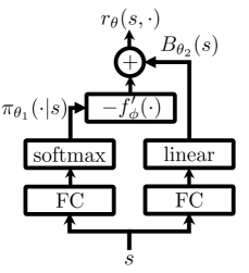
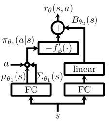
Figure 6: Density-based model for discrete (Left) and continuous control (Right)

J.3 Expert in Bermuda World environment

We assume a stochastic expert defined by

$$\pi_{\!{}_{E}}(a|s)=\frac{\sum_{t=1}^{3}(d^{(t)})^{-1}\mathbb{I}\{a=\mathrm{Proj}(\theta^{(t)})\}}{\sum_{t=1}^{3}(d^{(t)})^{-1}},$$

$$\theta^{(t)}=\operatorname{arctan2}(\bar{y}^{(t)}-y,\bar{x}^{(t)}-x),d^{(t)}=\|\bar{s}^{(t)}-s\|_{2}^{4}+\epsilon,t=1,2,3,$$

for $s=(x,y),\bar{s}^{(1)}=(\bar{x}^{(1)},\bar{y}^{(1)})=(-5,10),\bar{s}^{(2)}=(\bar{x}^{(2)},\bar{y}^{(2)})=(0,10),\bar{s}^{(3)}=(\bar{x}^{(3)},\bar{y}^{(3)})=(5,10)$, $\epsilon=10^{-4}$ and an operator $\mathrm{Proj}(\theta):\mathbb{R}\rightarrow\mathcal{A}$ that maps $\theta$ to the closest angle in $\mathcal{A}$. In Figure 7, we depicted the expert policy.

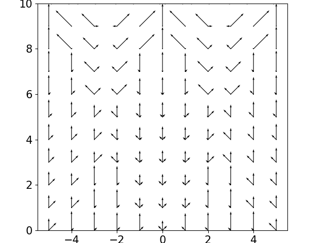
Figure 7: Visualization of the expert policy

J.4 MuJoCo experiment setting

Instead of directly using MuJoCo environments with $\mathrm{tanh}$-squashed policies proposed in Soft Actor-Critic (SAC) (Haarnoja et al., 2018), we move $\tanh$ to a part of environment—named hyperbolized environments in short—and assume Gaussian policies. Specifically, after an action $a$ is sampled from the policies, we pass $\mathrm{tanh}(a)$ to the environment. We then consider multi-variate Gaussian policy

$$\pi(\cdot|s)=\mathcal{N}\left(\boldsymbol{\mu}(s),\boldsymbol{\Sigma}(s)\right)$$

with $\boldsymbol{\mu}(s)=[\mu_{1}(s),...,\mu_{d}(s)]^{T}$, $\boldsymbol{\Sigma}(s)=\mathrm{diag}\{(\sigma_{1}(s))^{2},...,(\sigma_{d}(s))^{2}\}$, where

$$-\mathrm{arctanh}(0.99)\leq\mu_{i}(s)\leq\mathrm{arctanh}(0.99),\log(0.01)\leq\log\sigma_{i}(s)\leq\log(2)$$

for all $i=1,...,d$. Instead of using clipping, we use $\mathrm{tanh}$-activated outputs and scale them to be fit in the above ranges, which empirically improves the performance. Also, instead of using potential-based reward shaping used in AIRL (Fu et al., 2018), we update moving mean of intermediate reward values and update the value network with mean-subtracted rewards—so that the value network gets approximately mean-zero reward—to stabilize RL part of RAIRL. Note that this is motivated by Lemma 2 from which we can guarantee that any constant shift of reward functions does not change optimality.

J.5 Hyperparameters

Table LABEL:table:fixed_hyperparams_Bandit, Table LABEL:table:fixed_hyperparams_BermudaWorld and Table LABEL:table:fixed_hyperparams_MuJoCo list the parameters used in our Bandit, Bermuda World, and MuJoCo experiments, respectively.

Table 2: Hyperparameters for Bandit environments.

Hyper-parameter	Bandit
Batch size	500
Initial exploration steps	10,000
Replay size	500,000
Target update rate ($\tau$)	0.0005
Learning rate	0.0005
$\lambda$	5
$q$ (Tsallis entropy $\mathcal{T}_{q}^{k}$)	2.0
$k$ (Tsallis entropy $\mathcal{T}_{q}^{k}$)	1.0
Number of trajectories	1,000
Reward learning rate	0.0005
Steps per update	50
Total environment steps	500,000

Table 3: Hyperparameters for Bermuda World environment.

Hyper-parameter	Bermuda World
Batch size	500
Initial exploration steps	10,000
Replay size	500,000
Target update rate ($\tau$)	0.0005
Learning rate	0.0005
$q$ (Tsallis entropy $\mathcal{T}_{q}^{k}$)	2.0
$k$ (Tsallis entropy $\mathcal{T}_{q}^{k}$)	1.0
Number of trajectories	1,000
Reward learning rate	0.0005
(For evaluation) $\lambda$	1
(For evaluation) Learning rate	0.001
(For evaluation) Target update rate ($\tau$)	0.0005
Steps per update	50
Number of steps	500,000

Table 4: Hyperparameters for MuJoCo environments.

Hyper-parameter	Hopper	Walker2d	HalfCheetah	Ant
Batch size	256	256	256	256
Initial exploration steps	10,000	10,000	10,000	10,000
Replay size	1,000,000	1,000,000	1,000,000	1,000,000
Target update rate ($\tau$)	0.005	0.005	0.005	0.005
Learning rate	0.001	0.001	0.001	0.001
$\lambda$	0.0001	0.000001	0.0001	0.000001
$k$ (Tsallis entropy $\mathcal{T}_{q}^{k}$)	1.0	1.0	1.0	1.0
Number of trajectories	100	100	100	100
Reward learning rate	0.001	0.001	0.001	0.001
Steps per update	1	1	1	1
Number of steps	1,000,000	1,000,000	1,000,000	2,000,000

References

- Amari (2009) Shun-Ichi Amari. -divergence is unique, belonging to both -divergence and bregman divergence classes. IEEE Transactions on Information Theory, 55(11):4925–4931, 2009.
- Boularias & Chaib-Draa (2010) Abdeslam Boularias and Brahim Chaib-Draa. Bootstrapping apprenticeship learning. In Advances in Neural Information Processing Systems (NeurIPS), pp. 289–297, 2010.
- Bregman (1967) Lev M Bregman. The relaxation method of finding the common point of convex sets and its application to the solution of problems in convex programming. USSR computational mathematics and mathematical physics, 7(3):200–217, 1967.
- Csiszár (1963) Imre Csiszár. Eine informationstheoretische ungleichung und ihre anwendung auf den beweis der ergodizitat von markoffschen ketten. Magyar. Tud. Akad. Mat. Kutató Int. Közl, 8:85–108, 1963.
- Dadashi et al. (2020) Robert Dadashi, Léonard Hussenot, Matthieu Geist, and Olivier Pietquin. Primal wasserstein imitation learning. arXiv preprint arXiv:2006.04678, 2020.
- Finn et al. (2016a) Chelsea Finn, Paul Christiano, Pieter Abbeel, and Sergey Levine. A connection between generative adversarial networks, inverse reinforcement learning, and energy-based models. arXiv preprint arXiv:1611.03852, 2016a.
- Finn et al. (2016b) Chelsea Finn, Sergey Levine, and Pieter Abbeel. Guided cost learning: Deep inverse optimal control via policy optimization. In Proceedings of the 33rd International Conference on Machine Learning (ICML), pp. 49–58, 2016b.
- Fu et al. (2018) Justin Fu, Katie Luo, and Sergey Levine. Learning robust rewards with adverserial inverse reinforcement learning. In Proceedings of the 6th International Conference on Learning Representations (ICLR), 2018.
- Fujimoto et al. (2018) Scott Fujimoto, Herke Hoof, and David Meger. Addressing function approximation error in actor-critic methods. In Proceedings of the 35th International Conference on Machine Learning (ICML), pp. 1582–1591, 2018.
- Geist et al. (2019) Matthieu Geist, Bruno Scherrer, and Olivier Pietquin. A theory of regularized Markov decision processes. In Proceedings of the 36th International Conference on Machine Learning (ICML), pp. 2160–2169, 2019.
- Ghasemipour et al. (2019) Seyed Kamyar Seyed Ghasemipour, Richard Zemel, and Shixiang Gu. A divergence minimization perspective on imitation learning methods. In Proceedings of the 3rd Conference on Robot Learning (CoRL), 2019.
- Goodfellow et al. (2014) Ian Goodfellow, Jean Pouget Abadie, Mehdi Mirza, Bing Xu, David Warde Farley, Sherjil Ozair, Aaron Courville, and Yoshua Bengio. Generative adversarial nets. In Advances in Neural Information Processing Systems (NeurIPS), pp. 2672–2680, 2014.
- Guo et al. (2017) Xin Guo, Johnny Hong, and Nan Yang. Ambiguity set and learning via Bregman and Wasserstein. arXiv preprint arXiv:1705.08056, 2017.
- Haarnoja et al. (2018) Tuomas Haarnoja, Aurick Zhou, Pieter Abbeel, and Sergey Levine. Soft Actor-Critic: Off-policy maximum entropy deep reinforcement learning with a stochastic actor. In Proceedings of the 35th International Conference on Machine Learning (ICML), pp. 1861–1870, 2018.
- Ho & Ermon (2016) Jonathan Ho and Stefano Ermon. Generative adversarial imitation learning. In Advances in Neural Information Processing Systems (NeurIPS), pp. 4565–4573, 2016.
- Jones & Byrne (1990) Lee K Jones and Charles L Byrne. General entropy criteria for inverse problems, with applications to data compression, pattern classification, and cluster analysis. IEEE Transactions on Information Theory, 36(1):23–30, 1990.
- Ke et al. (2019) Liyiming Ke, Matt Barnes, Wen Sun, Gilwoo Lee, Sanjiban Choudhury, and Siddhartha Srinivasa. Imitation learning as -divergence minimization. arXiv preprint arXiv:1905.12888, 2019.
- Lee et al. (2018) Kyungjae Lee, Sungjoon Choi, and Songhwai Oh. Maximum causal tsallis entropy imitation learning. In Advances in Neural Information Processing Systems (NeurIPS), pp. 4403–4413, 2018.
- Lee et al. (2019) Kyungjae Lee, Sungyub Kim, Sungbin Lim, Sungjoon Choi, and Songhwai Oh. Tsallis reinforcement learning: A unified framework for maximum entropy reinforcement learning. arXiv preprint arXiv:1902.00137, 2019.
- Lee et al. (2020) Kyungjae Lee, Sungyub Kim, Sungbin Lim, Sungjoon Choi, Mineui Hong, Jaein Kim, Yong-Lae Park, and Songhwai Oh. Generalized Tsallis entropy reinforcement learning and its application to soft mobile robots. Robotics: Science and Systems Foundation, 2020.
- Li et al. (2018) Kun Li, Mrinal Rath, and Joel W Burdick. Inverse reinforcement learning via function approximation for clinical motion analysis. In 2018 IEEE International Conference on Robotics and Automation (ICRA), pp. 610–617. IEEE, 2018.
- Mescheder et al. (2017) Lars Mescheder, Sebastian Nowozin, and Andreas Geiger. Adversarial variational Bayes: Unifying variational autoencoders and generative adversarial networks. In Proceedings of the 34th International Conference on Machine Learning (ICML), pp. 2391–2400, 2017.
- Mnih et al. (2015) Volodymyr Mnih, Koray Kavukcuoglu, David Silver, Andrei A Rusu, Joel Veness, Marc G Bellemare, Alex Graves, Martin Riedmiller, Andreas K Fidjeland, Georg Ostrovski, et al. Human-level control through deep reinforcement learning. Nature, 518(7540):529–533, 2015.
- Mnih et al. (2016) Volodymyr Mnih, Adria Puigdomenech Badia, Mehdi Mirza, Alex Graves, Timothy Lillicrap, Tim Harley, David Silver, and Koray Kavukcuoglu. Asynchronous methods for deep reinforcement learning. In Proceedings of the 33rd International Conference on Machine Learning (ICML), pp. 1928–1937, 2016.
- Ng et al. (1999) Andrew Y Ng, Daishi Harada, and Stuart Russell. Policy invariance under reward transformations: Theory and application to reward shaping. In Proceedings of the 16th International Conference on Machine Learning (ICML), pp. 278–287, 1999.
- Ng et al. (2000) Andrew Y Ng, Stuart J Russell, et al. Algorithms for inverse reinforcement learning. In Proceedings of the 17th International Conference on Machine Learning (ICML), pp. 663–670, 2000.
- Nielsen & Nock (2011) Frank Nielsen and Richard Nock. On Rényi and Tsallis entropies and divergences for exponential families. arXiv preprint arXiv:1105.3259, 2011.
- Russell (1998) Stuart Russell. Learning agents for uncertain environments. In Proceedings of the 11th Annual Conference on Computational Learning Theory, pp. 101–103, 1998.
- Schulman et al. (2015) John Schulman, Sergey Levine, Pieter Abbeel, Michael Jordan, and Philipp Moritz. Trust region policy optimization. In Proceedings of the 32nd International Conference on Machine Learning (ICML), pp. 1889–1897, 2015.
- Schulman et al. (2017) John Schulman, Filip Wolski, Prafulla Dhariwal, Alec Radford, and Oleg Klimov. Proximal policy optimization algorithms. arXiv preprint arXiv:1707.06347, 2017.
- Sharifzadeh et al. (2016) Sahand Sharifzadeh, Ioannis Chiotellis, Rudolph Triebel, and Daniel Cremers. Learning to drive using inverse reinforcement learning and deep Q-networks. arXiv preprint arXiv:1612.03653, 2016.
- Stooke & Abbeel (2019) Adam Stooke and Pieter Abbeel. rlpyt: A research code base for deep reinforcement learning in pytorch. arXiv preprint arXiv:1909.01500, 2019.
- Syed et al. (2008) Umar Syed, Michael Bowling, and Robert E Schapire. Apprenticeship learning using linear programming. In Proceedings of the 25th International Conference on Machine Learning (ICML), pp. 1032–1039, 2008.
- Wu et al. (2020) Zheng Wu, Liting Sun, Wei Zhan, Chenyu Yang, and Masayoshi Tomizuka. Efficient sampling-based maximum entropy inverse reinforcement learning with application to autonomous driving. IEEE Robotics and Automation Letters, 5(4):5355–5362, 2020.
- Yang et al. (2019) Wenhao Yang, Xiang Li, and Zhihua Zhang. A regularized approach to sparse optimal policy in reinforcement learning. In Advances in Neural Information Processing Systems (NeurIPS), pp. 5938–5948, 2019.
- Zhang et al. (2019) Ruiyi Zhang, Bo Dai, Lihong Li, and Dale Schuurmans. GenDice: Generalized offline estimation of stationary values. In International Conference on Learning Representations, 2019.
- Ziebart (2010) Brian D Ziebart. Modeling purposeful adaptive behavior with the principle of maximum causal entropy. 2010.
- Ziebart et al. (2008) Brian D Ziebart, Andrew L Maas, J Andrew Bagnell, and Anind K Dey. Maximum entropy inverse reinforcement learning. In Proceedings of the 23rd AAAI Conference on Artificial Intelligence, volume 8, pp. 1433–1438, 2008.