Formation of dispersive shock waves in evolution of a two-temperature collisionless plasma

Abstract

The nonlinear dynamics of pulses in a two-temperature collisionless plasma with formation of dispersion shock waves is studied. An analytical description is given for arbitrary form of an initial disturbance with smooth enough density profile on a uniform density background. For large time after the wave breaking moment dispersive shock waves are formed. Motion of their edges is studied in framework of Gurevich-Pitaevskii theory and Whitham theory of modulations. The analytical results are compared with numerical solution.

I Introduction

The study of nonlinear waves is one of fascinating topics in modern science and it has attracted much attention in many various fields of research. In particular, it is now well known that a typical evolution of an initial pulse with a fairly smooth and large initial profile is accompanied by a gradual steepening followed by the wave breaking and formation of dispersive shock wave (DSW). The initial stage of evolution admits a purely hydrodynamic description where the classical Riemann method seems quite convenient (see, e.g., FRW-2009 ; IvanovKamchatnov-2019 ; IKP-2019 ; IKP-2019F ; IKP-2020 ). After the wave breaking moment the oscillatory wave structures emerge in the evolution of pulses and they are called “dispersive shock waves” or “undular bores”. Nowadays DSWs are recognized as a universal physical phenomenon encountered in diverse areas of science (see, e.g., kamch-2000 ; eh-2016 ). The notion of DSWs was introduced theoretically and demonstrated experimentally in water waves Bazin-65 ; DarcyBazin-65 ; BenjaminLighthill-54 , atmospheric layers SmythHolloway-88 ; Christie-92 ; HD-12 , Bose-Einstein condensates DBSH-01 ; secscb-05 ; KGK-04 ; hacces-06 , waves in magnetics magn-17 , intense electron beams MKFHBOT-13 , in nonlinear optics RG-89 ; WJF-07 ; Kodama-99 , and, most notably, in plasma ABS-68 ; TBI-70 ; GM-84 ; MS-63 ; Karpman-74 dynamics where DSWs were observed experimentally for the first time in the laboratory set up. Plasma shock waves have been studied in different plasma environments, such as ion-acoustic TBI-70 ; SN-05 ; Romagnani-08 ; BNS-08 , dust-ion-acoustic NBS-99 ; Nakamura-02 ; PGL-01 and in dusty multi-ion MCS-09 ; Duha-09 plasma. In this paper, we focus on theoretical description of ion-acoustic DSWs in a two-temperature collisionless plasma.

The simplest and, apparently, the most powerful theoretical approach to description of DSWs was formulated by Gurevich and Pitaevskii gp-73 in framework of the Whitham theory of modulation of nonlinear waves Whitham-65 ; Whitham-74 which was based on large difference between scales of the wavelength of nonlinear oscillations within DSW and the size of the whole DSW. In plasma physics applications, the dynamics of waves can be described by different wave equations, viz., Korteweg-de Vries (KdV) equation WashimiTaniuti-74 , KdV-Burgers (KdVB) equation MS-63 ; Sagdeev-66 , modified KdV (mKdV) ChanteurRaadu-87 , Gardner equation RTP-08 , nonlinear Schrödinger (NLS) equation Zakharov-72 , derivative NLS (DNLS) equation Rogister-71 ; Mjolhus-76 . For most of these equations (except for the KdVB equation) the corresponding modulation system can be reduced to a diagonal (Riemann) form. It is known that the possibility of diagonalization of the system of Whitham equations is closely related with their full integrability. However, although a large number of equations of nonlinear plasma physics are of this type, there are important situations when it is not the case and one has to resort to equations that are not completely integrable. A typical example of such a situation is presented by the nonlinear ion-sound waves (see, e.g., GM-84 ; gke-90-plasma ), and in these cases some development of the general theory of DSWs is required.

Apparently, the first general statement in this area was devised by Gurevich and Meshcherkin GM-84 , who proposed the condition which replaces the “jump condition” known in the theory viscous shocks. This condition is formulated in terms of Riemann invariants of the hydrodynamic system obtained in the dispersionless approximation of the original nonlinear wave equations under consideration. Typically, wave breaking occurs in the simple-wave flow when all physical variables of the system can be expressed as functions of only one of them what means that after transformation to the corresponding Riemann invariants only one of them breaks and the others remain constant. Gurevich and Meshcherkin claimed that this statement is correct also after formation of the DSW, so that flows at both its edges have the same values of the non-breaking Riemann invariants. This property is evidently correct in a simple case of self-similar solutions of Whitham equations for the KdV equation studied in gp-73 , when Whitham equations are transformed to the diagonal form, and Gurevich and Meshcherkin generalized it to situations when Riemann invariants of the modulation equations are unknown or even do not exist.

The next important success in this direction was achieved by G. El in Ref. El-05 , where it was noticed that the Whitham modulation equations degenerate at the DSW edges, where they match with the simple-wave dispersionless solution, into ordinary differential equations whose solutions provide the dependence of the DSW characteristics at the corresponding edge on a single parameter. This method made it possible to find the main parameters of DSWs arising due to evolution of the initial step-like discontinuities in many non-integrable situations including the case of ion-sound waves El-05 . Recently it was shown in Ref. Kamchatnov-19 that El’s method can be substantially generalized to arbitrary initial simple-wave conditions of the Gurevich-Meshcherkin class. When such a simple wave breaks, then, according to El El-05 , we know the limiting expressions for the characteristic velocities of the Whitham system at the DSW edges from simple physical considerations — they are equal either to the group velocity of the wave at the small-amplitude edge, or the soliton velocity at the soliton edge. This information, together with the known smooth solution of the dispersionless limit, is enough for finding the laws of motion of the corresponding edges of the DSW for an arbitrary initial profile of the simple-wave type. This approach was successfully used in IvanovKamchatnov-19 for theoretical description of DSWs in fully nonlinear theory of shallow water waves described by the Serre equation, and we will use here this method for finding the laws of motion of DSW edges in ion-acoustic DSWs.

The method of Refs. El-05 ; Kamchatnov-19 is based on the universal applicability of Whitham’s ‘number of waves conservation law’ Whitham-65 ; Whitham-74

$$\frac{\partial k}{\partial t}+\frac{\partial\omega(k)}{\partial x}=0,$$ (1)

Here $k=2\pi/L$ and $\omega=kV$ are the wave vector and the frequency of a linear harmonic wave $\propto\exp[i(kx-\omega t)]$ propagating along a smooth background, $L$ is the wavelength of the nonlinear periodic wave, $V$ being the phase velocity of the periodic wave. Long ago, Stokes noticed stokes (see also lamb ) that the solitons’s velocity can be found from the linear dispersion law because the soliton’s tails obey the same linearized equations and propagate with the same velocity as the whole soliton. This yields the expression for the soliton velocity $V_{s}={\widetilde{\omega}(\widetilde{k})}/{\widetilde{k}}$, where $\widetilde{\omega}(\widetilde{k})\equiv-i\omega(i\widetilde{k})$, $\widetilde{k}$ being the inverse half-width of the soliton. It is natural to suppose El-05 ; Kamchatnov-19 that for the simple-wave type of initial conditions the soliton counterpart of Eq. (1) is valid

$$\frac{\partial\widetilde{k}}{\partial t}+\frac{\partial\widetilde{\omega}(\widetilde{k})}{\partial x}=0.$$ (2)

El showed in Ref. El-05 that Eqs. (1) and (2) reduce at the corresponding edges of the DSW to the ordinary differential equations and their solutions gives at once the edges velocities of the DSW for the case of Gurevich-Pitaevskii initial step-like problem. This problem for the ion-acoustic case was solved in Refs. ekt-03 ; El-05 . In this paper, we generalize this theory to arbitrary form of the initial pulse and apply the method of Ref. Kamchatnov-19 to investigation of evolution of initial simple-wave ion-sound pulses.

The paper is structured as follows: the basic equations describing the dynamics of ion-acoustic waves in plasma are written out in Section II. The problem of the expansion of the initial hump of an ion density is considered in Section III and solved in the dispersionless approximation by the Riemann method. This solution can be applied to evolution of the pulse before the wave breaking moment. As is known, in the general case the initial pulse splits eventually to two pulses propagating in opposite directions, and each such a pulse can be represented as a simple wave so the method of Ref. Kamchatnov-19 becomes applicable. In Section IV, we find by this method the main characteristics of the DSW arising after breaking of a simple-wave.

II Main equations

We consider the system of equations which describe finite-amplitude ion-acoustic waves in a two-temperature ($T_{e}\gg T_{i}$) collisionless plasma Karpman-74 ; Sagdeev-1966 ; gke-90-plasma

$$\begin{split}&n_{T}+(nv)_{X}=0,\\ &v_{T}+vv_{X}+\frac{e}{m_{i}}\phi_{X}=0,\\ &\phi_{XX}=4\pi e\left(n_{0}\exp{\frac{e\phi}{T_{e}}}-n\right),\end{split}$$ (3)

where $n$ is the ion density, $v$ is the hydrodynamic velocity of the ions, $m_{i}$ is their mass, $\phi$ is the electric potential, $e$ and $T_{e}$ are the charge and temperature of electrons, and $n_{0}$ is the density of an undisturbed plasma. By means of replacements

$$\begin{split}t&=\Omega T,\quad x=D^{-1}X,\\ \rho&=\frac{n}{n_{0}},\quad u=\frac{v}{c_{s}},\quad\varphi=\frac{e}{T_{e}}\phi,\end{split}$$ (4)

where $\Omega=(4\pi e^{2}n_{0}/m_{i})^{1/2}$ is the ion plasma frequency, $D=(T_{e}/4\pi e^{2}n_{0})^{1/2}$ is the Debye length and $c_{s}^{2}=T_{e}/m_{i}$ is sound velocity, Eqs. (3) are transformed to a dimensionless form

$$\begin{split}&\rho_{t}+(\rho u)_{x}=0,\\ &u_{t}+uu_{x}+\varphi_{x}=0,\\ &\varphi_{xx}=e^{\varphi}-\rho.\end{split}$$ (5)

This system supports periodic traveling waves which have linear and solitary wave limits and also possesses at least four conservation laws gke-90-plasma . The harmonic dispersion law follows from linearized Eqs. (5)

$$\omega(k,\rho,u)=k\left(u+\frac{1}{\sqrt{1+k^{2}/\rho}}\right),$$ (6)

so that

$$\widetilde{\omega}(\widetilde{k},\rho,u)=\widetilde{k}\left(u+\frac{1}{\sqrt{1-\widetilde{k}^{2}/\rho}}\right).$$ (7)

In smooth flows, when the terms with higher space derivatives can be neglected, we arrive at the dispersionless limit with $\varphi=\ln{\rho}$, which yields the Euler isothermal gas-dynamic equations with the equation of state $p(\rho)=\rho$:

$$\begin{split}&\rho_{t}+(\rho u)_{x}=0,\\ &u_{t}+uu_{x}+\frac{\rho_{x}}{\rho}=0.\end{split}$$ (8)

The solution of such equations is greatly simplified if we pass from the ordinary physical variables $\rho$, $u$ to the so-called “Riemann invariants” (see, e.g., LandauLifshitz-1987 ). For Eqs. (8) the Riemann invariants are well known and can be written as

$$r_{\pm}=u\pm\ln{\rho}.$$ (9)

In these variables the hydrodynamic equations (8) take simple symmetric form

$$\frac{\partial r_{\pm}}{\partial t}+v_{\pm}(r_{-},r_{+})\frac{\partial r_{\pm}}{\partial x}=0,$$ (10)

where

$$v_{\pm}=u\pm 1$$ (11)

are the characteristic velocities of the system (8). They are expressed in terms of the Riemann invariants by the relations

$$v_{\pm}=\frac{1}{2}(r_{+}+r_{-})\pm 1.$$ (12)

These velocities coincide exactly with the corresponding limits of the Whitham velocities what guarantees a continuous matching of the dispersionless flows with the DSW at both its edges.

Having formulated the problem, we proceed to studying the dispersionless evolution of the plasma density pulse.

III Dispersionless solution

We assume that the initial state of plasma can be represented as a density hump on the constant uniform background and the density profile can be considered fairly smooth at the initial stage of evolution, so we turn to the system of hydrodynamic equations (8) or (10). Riemann noticed that Eqs. (10) can be linearized by the hodograph transform (see, e.g., Refs. kamch-2000 ; LandauLifshitz-1987 ) in which one considers $x$ and $t$ as functions of the independent variables $r_{\pm}$. This results in the following system of linear equations:

$$\begin{split}\frac{\partial x}{\partial r_{-}}-v_{+}(r_{-},r_{+})\frac{\partial t}{\partial r_{-}}&=0,\\ \frac{\partial x}{\partial r_{+}}-v_{-}(r_{-},r_{+})\frac{\partial t}{\partial r_{+}}&=0.\end{split}$$ (13)

It should be noticed that the Jacobian of this transformation is equal to

$$\begin{split}J=\left|\frac{\partial(x,t)}{\partial(r_{+},r_{-})}\right|=\frac{\partial t}{\partial r_{+}}\frac{\partial t}{\partial r_{-}}(v_{-}-v_{+}),\end{split}$$ (14)

and hence the hodograph transform breaks down whenever ${\partial t}/{\partial r_{+}}=0$ or ${\partial t}/{\partial r_{-}}=0$. This means that the hodograph transform is applicable only to the general solution, when both Riemann invariants are varying during the wave evolution. We look for the solution of the system (13) in the form

$$\begin{split}x-v_{+}(r_{-},r_{+})t&=w_{+}(r_{-},r_{+}),\\ x-v_{-}(r_{-},r_{+})t&=w_{-}(r_{-},r_{+}),\end{split}$$ (15)

where the functions $w_{\pm}$ are to be found. Then we get

$$\begin{split}t=-\frac{w_{+}-w_{-}}{v_{+}-v_{-}}.\end{split}$$ (16)

Differentiation of Eqs. (15) with respect to $r_{\pm}$ gives the relations $-\partial v_{\pm}/\partial r_{\mp}t=\partial w_{\pm}/\partial r_{\mp}$ and elimination of $t$ by means of (16) shows that the unknown functions $w_{\pm}(r_{+},r_{-})$ should satisfy the Tsarev equations Tsarev-1991

$$\begin{split}\frac{1}{w_{+}-w_{-}}\frac{\partial w_{+}}{\partial r_{-}}=\frac{1}{v_{+}-v_{-}}\frac{\partial v_{+}}{\partial r_{-}},\\ \frac{1}{w_{+}-w_{-}}\frac{\partial w_{-}}{\partial r_{+}}=\frac{1}{v_{+}-v_{-}}\frac{\partial v_{-}}{\partial r_{+}}.\end{split}$$ (17)

Now we notice that since the velocities $v_{\pm}$ are given by expressions (12), the right-hand sides of both Eqs. (17) are equal to each other:

$$\frac{1}{v_{+}-v_{-}}\frac{\partial v_{+}}{\partial r_{-}}=\frac{1}{v_{+}-v_{-}}\frac{\partial v_{-}}{\partial r_{+}}.$$ (18)

Consequently $\partial w_{+}/\partial r_{-}=\partial w_{-}/\partial r_{+}$ and $w_{\pm}$ can be sought in the form

$$w_{+}=\frac{\partial W}{\partial r_{+}},\quad w_{-}=\frac{\partial W}{\partial r_{-}}.$$ (19)

Substitution of Eqs. (18) and (19) into Eqs. (17) shows that the function $W$ obeys the Euler-Poisson equation

$$\frac{\partial^{2}W}{\partial r_{+}\partial r_{-}}-\frac{1}{4}\left(\frac{\partial W}{\partial r_{+}}-\frac{\partial W}{\partial r_{-}}\right)=0$$ (20)

A formal solution of Eq. (20) in the $(r_{+},r_{-})$ plane (the so-called hodograph plane) can be obtained with the use of the Riemann method (see, e.g., Sommerfeld-49 ; CourantHilbert-62 ).

In his fundamental paper Riemann-1860 , B. Riemann gave the following method of solving this problem. If we are interested in the value of the function $W$ at the point $P=(\xi,\eta)$ in the hodograph plane $(r_{+},r_{-})$, then we should draw in it from the point $P$ two characteristics ($r_{+}=\xi=\mathrm{const}$) and ($r_{-}=\eta=\mathrm{const}$), which together with the boundaries with known values of $W(r_{+},0)$ and $W(0,r_{-})$ along them form a closed contour $\mathcal{C}$ in this plane. The symbols $(\xi,\eta)$ denote here the coordinates of the “observation point” in the hodograph plane, whereas the notation $(r_{+},r_{-})$ is used for varying along the contour $\mathcal{C}$ coordinates. Riemann showed that $W(P)$ can be represented in the form

$$W(P)=\frac{1}{2}(R\overline{W})_{A}+\frac{1}{2}(R\overline{W})_{B}\pm\int_{A}^{B}(Vdr_{+}+Udr_{-}),$$ (21)

where the points $A$ and $B$ are projections of the “observation” point $P$ to $\mathcal{C}$ along the $r_{+}$ and $r_{-}$ axis respectively. Here

$$\begin{split}&U=\frac{1}{2}\left(R\frac{\partial\overline{W}}{\partial r_{-}}-\overline{W}\frac{\partial R}{\partial r_{-}}\right)-\frac{1}{4}\overline{W}R,\\ &V=\frac{1}{2}\left(\overline{W}\frac{\partial R}{\partial r_{+}}-R\frac{\partial\overline{W}}{\partial r_{+}}\right)-\frac{1}{4}\overline{W}R,\end{split}$$ (22)

where $\overline{W}$ denotes such a contraction of $W$ on the $\mathcal{C}$ curve; the functions $\overline{W}$ are known from the initial conditions for the problem under consideration. The function $R$ is called the Riemann function and it satisfies the equation

$$\frac{\partial^{2}R}{\partial r_{+}\partial r_{-}}+\frac{1}{4}\left(\frac{\partial R}{\partial r_{+}}-\frac{\partial R}{\partial r_{-}}\right)=0.$$ (23)

Besides that, Riemann imposed on it the following additional conditions:

$$\begin{split}\frac{\partial R}{\partial r_{+}}-\frac{1}{4}R=&0\quad\text{along the characteristic}\quad r_{-}=\eta,\\ \frac{\partial R}{\partial r_{-}}+\frac{1}{4}R=&0\quad\text{along the characteristic}\quad r_{+}=\xi,\\ \end{split}$$ (24)

and $R(\xi,\eta;\xi,\eta)=1$. These expressions suggest that $R$ can be looked for in the form

$$\begin{split}R=\exp{\left[\frac{1}{4}(r_{+}-\xi-r_{-}+\eta)\right]}F\left(r_{+},r_{-};\xi,\eta\right).\end{split}$$ (25)

Substituting it into Eq. (23), we obtain the Bessel equation for the function $F$, which shows that $R$ can be written in the form

$$\begin{split}\begin{split}R=&\exp{\left[\frac{1}{4}(r_{+}-\xi-r_{-}+\eta)\right]}\times\\ &\times I_{0}\left(\frac{1}{2}\sqrt{(r_{+}-\xi)(\eta-r_{-})}\right),\end{split}\end{split}$$ (26)

where $I_{0}$ is the Bessel function of complex argument (see, e.g., WhittakerWatson-1927 ).

We shall consider a typical initial distribution where $\rho(x,t=0)$ reaches an extremum value $\rho_{m}$ at $x=0$ and is an even function of $x$: $\rho(-x,t=0)=\rho(x,t=0)$. Such a pulse has the background density $\rho_{0}$ and characteristic width $l\gg\rho_{m}-\rho_{0}$ with $u(x,t=0)=0$. It is convenient to define the inverse functions of the initial $r_{\pm}$ profiles. The symmetry of the initial conditions makes it possible to use the same functions for $r_{+}\in[r_{0},r_{m}]$ and for $r_{-}\in[-r_{m},-r_{0}]$:

$$\begin{split}x(r_{\pm})=\begin{cases}\;\;\,\overline{x}(r_{\pm}),&\quad\text{if}\quad x>0,\\ -\overline{x}(r_{\pm}),&\quad\text{if}\quad x<0.\end{cases}\end{split}$$ (27)

We denote the Riemann invariant at the background as $r_{0}=r_{+}(x\rightarrow\pm\infty,t=0)$ and the initial maximum of Riemann invariant as $r_{m}=r_{+}(x=0,t=0)$.

Now the curve $\mathcal{C}$ is represented by the ‘antidiagonal’ $r_{-}=-r_{+}=-r$ along which Eqs. (15) with $t=0$ give

$$\overline{x}(r_{-})=\frac{\partial W}{\partial r_{-}},\quad\overline{x}(r_{+})=\frac{\partial W}{\partial r_{+}}.$$ (28)

Hence from

$$\overline{W}(\xi,\eta)=\int_{0}^{\xi}\overline{x}(r)dr+\int_{0}^{\eta}\overline{x}(r)dr$$ (29)

we get the necessary contraction of $W$ on $\mathcal{C}$. Then $\overline{W}(-r,r)=0$ and Eqs. (22) reduce to

$$U=\frac{1}{2}\overline{x}(r)R(r,-r;\xi,\eta),\quad V=-\frac{1}{2}\overline{x}(r)R(r,-r;\xi,\eta).$$ (30)

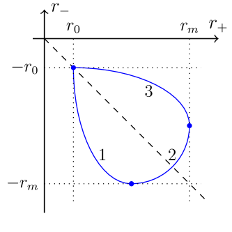
Figure 1: Characteristic plane ($r_{-},r_{+}$). The blue solid curve depicts the values of the Riemann invariants along the wave at fixed moment of time $t$.

It is convenient to divide $x$-axis into several domains (see IKP-2019 ; IKP-2019F ; IKP-2020 ) which correspond to specific behavior of the Riemann invariants in each domain. For a general solution, we numerate these regions by the Arabic numbers $1$, $2$, and $3$. In region $1$, the Riemann invariant $r_{+}$ is an increasing function of $x$, and the Riemann invariant $r_{-}$ is a decreasing function of $x$. In region $2$, both Riemann invariants increase. In region $3$ invariant $r_{+}$ decreases, and $r_{-}$ increases. Each of these regions requires its own treatment. The Fig. 1 shows the hodograph plane $(r_{+},r_{-})$-axes. Here, different regions of the general solution are indicated by various Arabic numerals. For each such a region, the solution of the Euler-Poisson equation (20) $W$ has its own expression. To find each of these expressions, we, following Ludford Ludford-52 , unfold the domain $[r_{0},r_{m}]\times[-r_{m},-r_{0}]$ into a four times larger region as is shown in Fig. 2.

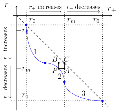
Figure 2: The unfolded hodograph plane ($r_{-},r_{+}$). The blue solid curve depicts the values of the Riemann invariants along the wave at fixed moment of time $t$.

The potential $W(r_{+},r_{-})$ takes different forms in each of the regions labeled $1$, $2$, and $3$ in Fig. 2 and can be considered as a single valued function on the unfolded plane. Thus, from Eq. (21) we obtain $W$ in the regions $1$ and $3$

$$\begin{split}W^{(1)}(\xi,\eta)=-W^{(3)}(\xi,\eta)=-\int_{-\eta}^{\xi}\overline{x}(r)R(r,-r;\xi,\eta)dr.\end{split}$$ (31)

For the region $2$ after integration by parts we obtain

$$\begin{split}W^{(2)}(\xi,\eta)&=\left(RW^{(1)}\right)_{B}+\left(RW^{(3)}\right)_{A}\\ &+\int_{A}^{C}\left.\left(\frac{\partial R}{\partial r_{-}}-aR\right)\right|_{r_{+}=r_{m}}W^{(3)}dr_{-}\\ &-\int_{C}^{B}\left.\left(\frac{\partial R}{\partial r_{+}}-bR\right)\right|_{r_{-}=-r_{m}}W^{(1)}dr_{+},\end{split}$$ (32)

where the coordinates of the relevant points are equal to $A=(r_{m},\eta)$, $B=(\xi,-r_{m})$ and $C=(r_{m},-r_{m})$ (see Fig. 2).

In practice, it is convenient to use an approximation suggested in Refs. IKP-2019 ; IKP-2019F ; IKP-2020 . It consists of the assumption the argument of the Bessel function in Eq. (26) is small and, consequently, the Riemann function reduces to the expression

$$\begin{split}R(r_{+},r_{-};\xi,\eta)&\simeq R(r_{+}-r_{-},\xi-\eta)\\ &=\exp{\left[\frac{1}{4}(r_{+}-\xi-r_{-}+\eta)\right]}.\end{split}$$ (33)

In the case of applicability of this approximation, we obtain in regions $1$ and $3$

$$\begin{split}W^{(1)}&(r_{-},r_{+})=-W^{(3)}(r_{-},r_{+})\\ &=\int_{-r_{-}}^{r_{+}}\overline{x}(r)R(2r;r_{+}-r_{-})dr,\\ \end{split}$$ (34)

and in region $2$

$$\begin{split}W&{}^{(2)}(r_{-},r_{+})\\ &=R(r_{m},-r_{-};r_{+}-r_{-})\int_{-r_{-}}^{r_{m}}\overline{x}(r)R(2r,r_{m}-r_{-})dr\\ &+R(r_{+}+r_{m},r_{+}-r_{-})\int_{r_{+}}^{r_{m}}\overline{x}(r)R(2r,r_{+}+r_{m})dr,\end{split}$$ (35)

where we have made the replacements $\xi\rightarrow r_{+}$, $\eta\rightarrow r_{-}$ to return to the notation of Eqs. (15) and (19). When $W$ is known, we can find from (15) the Riemann invariants as functions of $x$ and $t$, and then the physical variables are expressed by the formulas

$$\begin{split}\rho=\exp{\left[\frac{1}{2}(r_{+}-r_{-})\right]},\qquad u=\frac{1}{2}(r_{+}+r_{-}).\end{split}$$ (36)

At the edges of a finite evolving pulse, the simple-waves regions arise with one of the Riemann invariants constant. We label such regions by Roman numerals: the region where the Riemann invariant $r_{-}$ decreases and the Riemann invariant $r_{+}$ remains constant we denote as $I$; the label $II_{l}$ corresponds to the region where $r_{-}$ increases and $r_{+}$ remains constant; at last, at the right edge of the momentum, we denote the regions where $r_{-}$ remains constant and the Riemann invariant $r_{+}$ increases and decreases as $III$ and $II_{r}$, respectively.

In the simple-wave regions, where one of the Riemann invariants is constant, the hodograph transform is not valid. At the initial stages of evolution, when the regions $I$ and $III$ do exist, we look for the simple wave solution in the form

$$\begin{split}&x-v_{-}(r_{-},r_{0})t=h(r_{-}),\qquad\text{for region $I$},\\ &x-v_{+}(-r_{0},r_{+})t=h(r_{+}),\qquad\text{for region $III$},\end{split}$$ (37)

where the function $h$ is determined by the boundary conditions of matching of the intensity at the boundary between the simple wave and the general solution (see Eqs. (15)). Thus we have

$$\begin{split}x-v_{-}(r_{-},r_{0})t=\frac{\partial W^{(1)}(r_{-},r_{0})}{\partial r_{-}},\end{split}$$ (38)

for the simple-wave region $I$ and

$$\begin{split}x-v_{+}(-r_{0},r_{+})t=\frac{\partial W^{(3)}(-r_{0},r_{+})}{\partial r_{+}},\end{split}$$ (39)

for the region $III$.

After a certain time of evolution the two simple-wave regions are formed, which are denoted as $II_{l}$ and $II_{r}$. Similarly, we can get

$$\begin{split}x-v_{+}(-r_{0},r_{+})t=\frac{\partial W^{(2)}(-r_{0},r_{+})}{\partial r_{+}},\end{split}$$ (40)

for the region $II_{l}$ and

$$\begin{split}x-v_{-}(r_{-},r_{0})t=\frac{\partial W^{(2)}(r_{-},r_{0})}{\partial r_{+}},\end{split}$$ (41)

for the region $II_{r}$.

Thus we obtain the complete description of the dispersionless wave evolution.

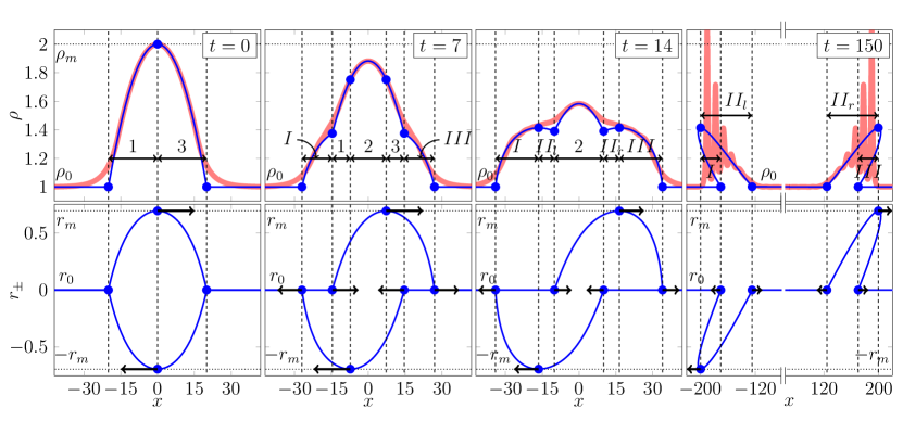
Figure 3: (Top row) Density $\rho$ versus coordinate $x$. A comparison of the analytical solution (blue thin curve) and direct numerical solution of Eqs. 5 (red thick curve) for different $t$ is shown. The initial state has a parabolic shape and it is shown in the left panel. The Arabic numerals denote the regions of the general solution, and the Roman numerals indicate the regions of simple waves. (Bottom row) The dependence of the Riemann invariants $r_{\pm}$ on the spatial coordinate $x$ at the same moments of time. The right column corresponds to the time after the wave-breaking with formation of a multi-valued dispersionless solution.

Figure 4: Diagram of the Riemann invariant on the unfolded hodograph plane $(r_{+},r_{-})$ for the initial state (42). Different colors indicate curves at different moments in time. The region above the red line is unreachable for the initial distribution under consideration.

We shall illustrate the above theory by the example with a parabolic initial distribution of the density

$$\begin{split}\rho(x,t=0)=\begin{cases}\rho_{0}+(\rho_{m}-\rho_{0})(1-\frac{x^{2}}{l^{2}}),&\quad|x|\leq l,\\ \rho_{0},&\quad|x|>l,\end{cases}\end{split}$$ (42)

where $l$ is a characteristic width of the distribution and the initial flow velocity is equal to zero, $u(x,t=0)=0$ (see left panel on the top row of Fig. 3). For these conditions the inverse function of $r(x,t=0)$ (see left panel on the bottom row of Fig. 3) for the positive branch has the form

$$\overline{x}(r)=l\sqrt{\frac{\rho_{m}-e^{r}}{\rho_{m}-\rho_{0}}}.$$ (43)

As one can see from Fig. 3, two simple-wave regions $I$ and $III$ appear in the course of evolution, as well as a region of general solution, which is labeled by ${2}$. Next, regions $1$ and $3$ vanish, and new simple wave regions $II_{l}$ and $II_{r}$ appear (third column of Fig. 3). For longer time (right column of Fig. 3), region 2 also vanishes and only simple-wave regions persist: the initial pulse splits into two simple-wave pulses propagating in opposite directions. The corresponding curves on a four-sheeted hodograph plane are shown in the Fig. 4.

Substitution of the initial conditions into our approximate expressions (34) and (35) for $W$ yields

$$\begin{split}W^{(1)}&(r_{-},r_{+})=-W^{(3)}(r_{-},r_{+})\\ &=-\left(\varPhi(r_{+},r_{+},r_{-})-\varPhi(-r_{-},r_{+},r_{-})\right),\\ W^{(2)}&(r_{-},r_{+})=R(r_{m}-r_{-},r_{+}-r_{-})\\ &\times\left(\varPhi(r_{m},r_{m},r_{-})-\varPhi(-r_{-},r_{m},r_{-})\right)\\ &+R(r_{+}+r_{m},r_{+}-r_{-})\\ &\times\left(\varPhi(r_{m},r_{+},-r_{m})-\varPhi(r_{+},r_{+},-r_{m})\right),\end{split}$$ (44)

where

$$\begin{split}\varPhi(r,\xi,\eta)&=\frac{l}{\sqrt{\rho_{m}-\rho_{0}}}\exp{\left(-\frac{\xi-\eta}{4}\right)}\\ &\times\left(e^{r/2}\sqrt{\rho_{m}-e^{r}}+\rho_{m}\arcsin{\frac{e^{r/2}}{\sqrt{\rho_{m}}}}\right).\end{split}$$

Once $r_{+}$ and $r_{-}$ have been determined as functions of $x$ and $t$ using (44) and (16), the density and velocity profiles are calculated by means of Eqs. (36). One obtains a quite exact description of the initial dispersionless stage of evolution of the pulse, as is demonstrated in the top row of Fig. 3. At larger time, the density profile at both edges of the pulse steepens, DSWs are formed and the amplitude of these oscillations accordingly increases. The dispersionless approximation subsequently predicts a nonphysical multi-valued profile, as can be seen in right column of Fig. 3. It is worth noticing that the wave breaking leads to overlapping of the regions. An example of such a solution is shown in the right column of Fig. 4. One can see that two simple-wave regions ($I$ and $II_{l}$ or $II_{r}$ and $III$) overlap. We shall not consider this phenomenon in detail now, since such multi-valued regions are nonphysical and, when dispersion is taken into account, they are replaced by DSWs.

IV Dispersive shock wave formation

We have shown that any localized initial pulse with initial distributions of $\rho(x,0)$, $u(x,0)$ different from some constant values $\rho_{0}$, $u_{0}=0$ on a finite interval of $x$ evolves eventually into two separate pulses propagating in opposite directions. These two pulses are called simple-wave solutions in which one of the Riemann invariants $r_{\pm}$ is constant. Further evolution leads to steepening of the wave profile and wave breaking followed by formation of a DSW. Here, in this section, we suppose that the initial state belongs to such a class of simple waves. To be definite, we assume that $r_{-}=u-\ln\rho=-\ln\rho_{0}=\mathrm{const}$, that is we consider the right-propagating wave with

$$\rho=\rho_{0}e^{u},\quad r_{+}=2u+\ln\rho_{0},$$ (45)

so that the solution of dispersionless equations can be written as

$$x-(u+1)t=\overline{x}(u),$$ (46)

where $\overline{x}(u)$ is the function inverse to the initial distribution of the local flow velocity. Thus, we consider the wave breaking in terms of the flow velocity $u$.

IV.1 Positive Pulse

We shall start with a monotonous pulse with the initial distribution

$$u(x,0)=\begin{cases}\widetilde{u}(x)&\mbox{if}\quad x<0,\\ 0&\mbox{if}\quad x\geq 0,\end{cases}$$ (47)

where $\widetilde{u}(x)$ monotonously increases with decrease of $x$; see Fig. 5(a). We can see at once that if the initial distribution of the flow velocity $u$ has the form of a hump (“positive pulse”), then the wave breaking occurs at the front of the pulse with formation of solitons at the front edge of the DSW and with small-amplitude edge at the boundary with the smooth part of the pulse described by Eq. (46) (rear edge of the DSW). Therefore, our task here is to find the law of motion of the small-amplitude edge by the method of Ref. Kamchatnov-19 .

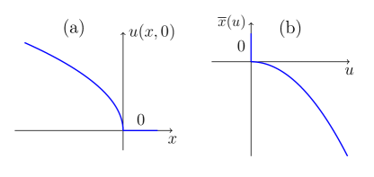
Figure 5: (a) Monotonous positive initial condition and (b) the inverse function $\overline{x}(u)$.

To this end, we have to solve the number of waves conservation law equation (1) where $k=k(u)$ is an unknown function to be found. Actually, it was done in El-05 , and we reproduce here briefly the necessary results in a convenient for us form. We represent the dispersion relation (6) in the form

$$\omega(k)=k[u+\alpha(k)],$$ (48)

that is the function

$$\alpha(k)=\frac{1}{\sqrt{1+k^{2}/\rho}},\qquad(0<\alpha<1),$$

measures deviation of the dispersion law from a linear non-dispersive limit, and then we have

$$k(u)=\sqrt{\rho_{0}e^{u}\left(\frac{1}{\alpha^{2}}-1\right)},$$ (49)

where $\alpha=\alpha(u)$ is an unknown yet function.

With the use of the equation

$$\frac{\partial u}{\partial t}+(u+1)\frac{\partial u}{\partial x}=0$$ (50)

corresponding to one of the limiting characteristic velocities of the Whitham system and equivalent to Eq. (10) for $r_{+}$, we reduce Eq. (1) to the ordinary differential equation

$$\frac{d\alpha}{du}=-\frac{\alpha(1+\alpha)^{2}}{2(1+\alpha+\alpha^{2})},$$ (51)

which coincides with the equation obtained in Ref. El-05 . It has to be solved with the boundary condition

$$\alpha(0)=1,$$ (52)

which means that the distance between solitons tends to infinity at the soliton edge, hence $k(u)\to 0$ as $u\to 0$. Integration of Eq. (51) with the boundary condition (52) is elementary and yields

$$u(\alpha)=-2\ln\alpha-\frac{1-\alpha}{1+\alpha}.$$ (53)

Now, we can find the law of motion of the small-amplitude edge of the DSW which propagates with the group velocity equal to, as one can easily obtain,

$$s_{L}=\frac{d\omega}{dk}=u(\alpha)+\alpha^{3}.$$ (54)

The small-amplitude edge matches the dispersionless solution (46). Along the path of the small-amplitude edge we have $dx-s_{L}dt=0$, i.e., $x=x_{L}(u)$ and $t=t(u)$ satisfy the equation

$$\frac{\partial x}{\partial u}-s_{L}\frac{\partial t}{\partial u}=0.$$ (55)

This equation must be compatible with Eq. (46) and this condition yields the equation

$$(\alpha^{3}-1)\frac{dt}{du}-t=\frac{d\overline{x}}{du}$$ (56)

for the function $t=t(u)$, where $\overline{x}(u)$ is the function inverse to the initial distribution of $u(x)$; see Fig. 5(b). Since we already know the relationship (53) between $u$ and $\alpha$, it is convenient to transform Eq. (56) to the independent variable $\alpha$. To simplify the notation, we introduce the function

$$\Phi(\alpha)=\left.\frac{d\overline{x}}{d\alpha}\right|_{u=u(\alpha)}$$ (57)

and obtain

$$\frac{\alpha}{2}(1-\alpha)(1+\alpha)^{2}\frac{dt}{d\alpha}-t=\Phi(\alpha).$$ (58)

Its solution with the initial condition $t(0)=0$ reads

$$\begin{split}t(\alpha)&=2\exp{\left[\frac{1}{1+\alpha}\right]}\frac{\alpha^{2}}{(1-\alpha)^{1/2}(1+\alpha)^{3/2}}\\ &\times\int_{1}^{\alpha}\frac{\Phi(z)\exp{(-1/(1+z))}}{z^{3}\sqrt{1-z^{2}}}dz\end{split}$$ (59)

and, consequently,

$$x_{L}(\alpha)=[u(\alpha)+1]t(\alpha)+\overline{x}[u(\alpha)].$$ (60)

The formulas (59) and (60) define in a parametric form the law of motion $x=x_{L}(t)$ of the small-amplitude edge.

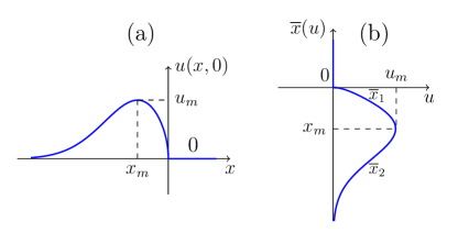
Figure 6: (a) Localized positive initial pulse; (b) the inverse function $\overline{x}(u)$ is represented by two branches $\overline{x}_{1}(u)$ and $\overline{x}_{2}(u)$.

In the case of a localized initial pulse shown in Fig. 6 the inverse function becomes two-valued and we denote its two branches as $\overline{x}_{1}(u)$ and $\overline{x}_{2}(u)$. The initial distribution $u(x)$ has a single maximum $u_{m}$ at $x=x_{m}$ and $u(x)\to 0$ fast enough as $x\to-\infty$ and $u(x)\to 0$ with vertical tangent line at $x\to-0$. The above formulas obtained for monotonous initial distribution are applicable as long as the small-amplitude edge propagates along the branch $\overline{x}_{1}(u)$, so that the solution can be derived by replacement of the function $\Phi(\alpha)$ by $\Phi_{1}(\alpha)=\left.d\overline{x}_{1}/du\right|_{u=u(\alpha)}$. When the small-amplitude edge reaches the maximum $u_{m}$ at the moment $t_{m}$, then the equation (58) with $\Phi(\alpha)$ replaced by $\Phi_{2}(\alpha)=\left.d\overline{x}_{2}/du\right|_{u=u(\alpha)}$ should be solved with the boundary condition $t(\alpha_{m})=t_{m},$ where $\alpha_{m}$ is the root of the equation $u(\alpha_{m})=u_{m}$. Hence, for $t>t_{m}$ the motion of the small-amplitude is determined by the formula

$$\begin{split}t(\alpha)&=2\exp{\left[\frac{1}{1+\alpha}\right]}\frac{\alpha^{2}}{(1-\alpha)^{1/2}(1+\alpha)^{3/2}}\\ &\times\left(\int_{1}^{\alpha_{m}}\frac{\Phi_{1}(z)\exp{(-1/(1+z))}}{z^{3}\sqrt{1-z^{2}}}dz+\right.\\ &\qquad\left.\int_{\alpha_{m}}^{\alpha}\frac{\Phi_{2}(z)\exp{(-1/(1+z))}}{z^{3}\sqrt{1-z^{2}}}dz\right).\end{split}$$ (61)

The law of motion of the soliton edge of DSW cannot be found by this method, since the relation (2) does not hold during evolution of the pulse. However, as was remarked in Ref. Kamchatnov-19 , this relationship can be used in vicinity of the moment when the small-amplitude edge reaches the point with $u=u_{m}$. We write the soliton dispersion law (7) in the form

$$\widetilde{\omega}(\widetilde{k})=\widetilde{k}[u+u\widetilde{\alpha}(\widetilde{k})],$$ (62)

that is

$$\widetilde{\alpha}(\widetilde{k})=\frac{1}{\sqrt{1-\widetilde{k}^{2}/\rho}},\qquad(\widetilde{\alpha}>1),$$

Substitution of Eq. (62) together with

$$\widetilde{k}(c)=\sqrt{\rho_{0}e^{u}\left(1-\frac{1}{\alpha^{2}}\right)}.$$ (63)

into Eq. (2) gives

$$\frac{d\widetilde{\alpha}}{du}=-\frac{\widetilde{\alpha}(1+\widetilde{\alpha})}{2(1+\widetilde{\alpha}+\widetilde{\alpha}^{2})},$$ (64)

which, according El’s approach, should be solved with the boundary condition

$$\widetilde{\alpha}(u_{m})=1,$$ (65)

which means that the solitons widths become infinitely large ($\widetilde{k}\to 0$) and their amplitude is infinitely small at the small-amplitude edge. As a result, we get

$$u(\widetilde{\alpha})=u_{m}-2\ln\widetilde{\alpha}-\frac{1-\widetilde{\alpha}}{1+\widetilde{\alpha}}$$ (66)

and

$$s_{R}=\left.\frac{\widetilde{\omega}}{\widetilde{k}}\right|_{u=0}=\widetilde{\alpha}(0).$$ (67)

Here $u<u_{m}$, $\widetilde{\alpha}$ increases with decrease of $u$ and reaches its maximal value at $u=0$. This value of the leading soliton velocity in DSW is reached at large enough time when solitons near the leading edge are well separated from each other.

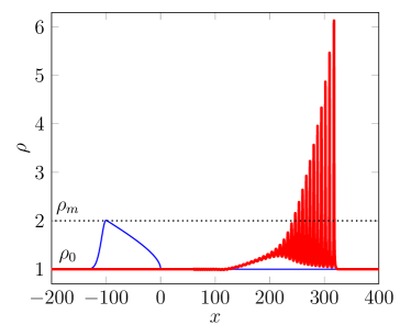
Figure 7: Simple-wave initial state (68) with $\rho_{0}=1$, $x_{0}=-100$ and $B=0.07$ is shown by the blue (thin) solid curve. Density profile at $t=250$ is shown by the red (thick) solid curve).

We have compared our analytical approach with numerical simulations of the Eqs. (5). We have chosen the initial condition in the form

$$\begin{split}u(x,t=0)=\begin{cases}A\exp{\left(-\frac{(x-x_{0})^{2}}{4\delta(x_{0}-\delta)}\right)},&\quad\text{if}\quad x\leq\delta,\\ B\sqrt{-x},&\quad\text{if}\quad x>\delta,\end{cases}\end{split}$$ (68)

where

$$A={B}\;\exp{\left(-\frac{1}{4}\left(1-\frac{x_{0}}{\delta}\right)\right)}{\sqrt{-\delta}}\;,\quad\delta=x_{0}+0.5.$$

So that density distribution has the form (see blue (thin) curve in Fig. 7)

$$\begin{split}\rho=\rho_{0}e^{u(x,t=0)}.\end{split}$$ (69)

This initial state is split into two branches as shown in the Fig. 6. The typical form of the DSW generated by such a pulse is represented in the same figure by a red (thick) curve. Eqs. (60) and (61) give the parametrical dependence of the small-amplitude edge of the DSW $x=x_{L}(t)$ shown in Fig. 8 by a blue solid curve. As we can see, it agrees reasonably well with the result of numerical solution shown by a red dots. We determine the position of small-amplitude edge numerically by means of an approximate extrapolation of the envelopes of the wave at this edge. For the right solitonic edge of the DSW, we can find the asymptotic propagation velocity, which for a given initial state is approximately equal to $s_{R}=1.59$ and is shown in Fig. 9 by a dashed line. Fig. 9 shows that the numerically determined velocity of a given edge tends to the asymptotic analytical value $s_{R}$.

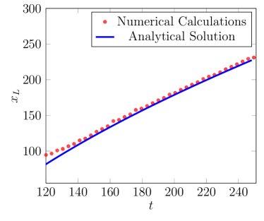
Figure 8: Comparison of the numerical solution of Eqs. (5) (red dots) and the analytical parametric solution (60) and (61) (blue (solid) curve) for the small-amplitude edge of DSW. The initial state parameters are indicated in the caption Fig. 7.

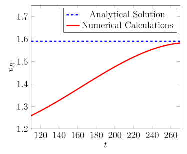
Figure 9: Velocity of the soliton edge as a function of time (red (solid) line). Blue (dashed) line indicates the asymptotic value of the velocity of this edge given by Eq. (67).

IV.2 Number of solitons

For asymptotically large time $t\to\infty$, a localized pulse shown in Fig. 6(a) transforms into a train of bright solitons and we have found the velocity (67) of the leading soliton. Another important characteristic of this evolution is the number $N$ of solitons produced from a pulse with a given initial distribution $u_{0}(x)=u(x,0)$. To calculate this number $N$, we turn to an important remark made by Gurevich and Pitaevskii in gp-87 that the number of waves entering per unit of time into the DSW region at its small-amplitude edge is given by

$$\frac{dN}{dt}=\frac{1}{2\pi}\left(k\frac{\partial\omega}{\partial k}-\omega\right),$$ (70)

where the right-hand side is calculated at the values of the small-amplitude edge parameters at the moment of time $t$. According to Eq. (1), the frequency $\omega(k)/(2\pi)$ plays the role of the flux of the number of waves, so the right-hand side of Eq. (70) can be interpreted as a flux calculated with account of Doppler shift due to motion of the edge with the group velocity $d\omega/dk$.

If we consider a localized initial pulse, then all waves inside the DSW transform eventually into solitons and their number is given by the integral kamch-20b

$$N=\frac{1}{2\pi}\int_{0}^{\infty}\left(k\frac{\partial\omega}{\partial k}-\omega\right)dt.$$ (71)

Since the function $k(\alpha)$ is defined by Eqs. (49), (53), and $t(\alpha)$ is given by (59), (61), this integral can be calculated directly. However, it is instructive to transform it much simpler form. To this end we substitute the above formulas into (71) to get

$$\begin{split}&N=\frac{1}{\pi}\int_{\alpha_{m}}^{1}\exp\left(-\frac{1-\alpha}{2(1+\alpha)}\right)\frac{\sqrt{1-\alpha^{2}}}{\alpha^{2}(1+\alpha)}\times\\ &\times\Bigg{\{}2\exp\left(\frac{1}{1+\alpha}\right)\frac{\alpha^{2}}{(1-\alpha)^{1/2}(1+\alpha)^{3/2}}\times\\ &\times\int_{\alpha_{m}}^{\alpha}\frac{(\Phi_{2}-\Phi_{1})e^{-\frac{1}{1+z}}dz}{z^{3}\sqrt{1-z^{2}}}+\Phi_{2}(\alpha)-\Phi_{1}(\alpha)\Bigg{\}}d\alpha.\end{split}$$ (72)

We notice that the double integral here can be reduced to the ordinary one by integration by parts and after collecting all terms and some simplifications we obtain

$$N=\frac{1}{\pi}\int_{\alpha_{m}}^{1}e^{-\frac{1-\alpha}{2(1+\alpha)}}(\Phi_{2}-\Phi_{1})\frac{1+\alpha+\alpha^{2}}{\alpha^{3}(1+\alpha)^{2}}d\alpha.$$ (73)

Now, taking into account the definition (57) of $\Phi$, Eq. (51), and the initial condition $\overline{x}(\alpha)=-2\ln\alpha-\frac{1-\alpha}{1+\alpha}$ obtained from (53) at $t=0$, we arrive at the final result

$$N=\frac{1}{2\pi}\int_{-\infty}^{0}k[u_{0}(x)]dx,$$ (74)

where $k(u)$ is defined in Eq. (49). This formula has a general nature. It was suggested in Refs. egkkk-07 ; egs-08 as a consequence of continuation of solution of the Whitham modulation equations to the dispersionless region. For some other equations it was justified by a similar calculations in Ref. kamch-20b .

IV.3 Negative pulse

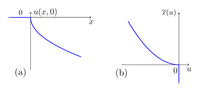
Figure 10: (a) Monotonous negative initial condition; (b) the inverse function $\overline{x}(u)$.

Now we turn to the situation sketched in Figs. 10(a) with a monotonous pulse in the initial distribution of the velocity

$$u(x,0)=\begin{cases}0&\mbox{if}\quad x<0,\\ -\widetilde{u}(x)&\mbox{if}\quad x\geq 0,\end{cases}$$ (75)

The inverse function $\overline{x}(u)$ is shown in Fig. 10(b). As was indicated in Ref. Kamchatnov-19 , in situations of this kind Eq. (46) is fulfilled at the soliton edge located at the boundary with the smooth part of the pulse which is described in dispersionless approximation by Eq. (46). The small-amplitude edge of the DSW is located at the boundary with the quiescent medium where $u=u_{0}=0$. Eq. (2) can be transformed in the same way as it was done in Eqs. (62)-(64), but now Eq. (64) must be solved with the boundary condition

$$\widetilde{\alpha}(0)=1.$$ (76)

This gives

$$u(\widetilde{\alpha})=-2\ln\widetilde{\alpha}-\frac{1-\widetilde{\alpha}}{1+\widetilde{\alpha}},$$ (77)

where $\widetilde{\alpha}>1$, and consequently the trailing soliton velocity is equal to

$$s_{R}=\frac{\widetilde{\omega}}{\widetilde{k}}=u(\widetilde{\alpha})+\widetilde{\alpha}.$$ (78)

It corresponds to the characteristic velocity of the limiting Whitham equation

$$\frac{\partial x}{\partial u}-[u(\widetilde{\alpha})+\widetilde{\alpha}]\frac{\partial t}{\partial u}=0.$$ (79)

The condition that this equation must be compatible with the solution (46) of the dispersionless approximation at the soliton edge of the DSW yields the differential equation for the function $t=t(u)$ at this edge,

$$(\widetilde{\alpha}-1)\frac{dt}{du}-t=\frac{d\overline{x}}{du}.$$ (80)

Introducing the function $\Phi(\widetilde{\alpha})=\left.d\overline{x}/du\right|_{u=u(\widetilde{\alpha})}$ we cast it to the form

$$\frac{\widetilde{\alpha}(\widetilde{\alpha}-1)(\widetilde{\alpha}+1)^{2}}{2(1+\widetilde{\alpha}+\widetilde{\alpha}^{2})}\frac{dt}{d\widetilde{\alpha}}+t=-\Phi(\widetilde{\alpha})$$ (81)

with $\widetilde{\alpha}$ as an independent variable. Since we assume that the initial profile breaks at the moment $t=0$ at the rear edge where $u=u_{0}$, i.e., $\widetilde{\alpha}=1$, this equation should be solved with the boundary condition

$$t(1)=0.$$ (82)

As a result, we obtain

$$\begin{split}t(\widetilde{\alpha})&=\frac{2\widetilde{\alpha}^{2}}{(\widetilde{\alpha}-1)^{3/2}(\widetilde{\alpha}+1)^{1/2}}\exp{\left[\frac{1}{\widetilde{\alpha}+1}\right]}\times\\ \times&\int_{1}^{\widetilde{\alpha}}\Phi(z)\frac{(z-1)^{1/2}(1+z+z^{2})}{z^{3}(z+1)^{3/2}}\exp{\left[-\frac{1}{z+1}\right]}dz.\end{split}$$ (83)

The coordinate of the soliton edge is given by

$$x_{R}(\widetilde{\alpha})=[u(\widetilde{\alpha})+1]t(\widetilde{\alpha})+\overline{x}[u(\widetilde{\alpha})],$$ (84)

so that Eqs. (83), (84) define the law of motion $x=x_{R}(t)$ of this edge in parametric form. Generalization of this theory on localized pulses (see Fig. 11) is straightforward.

At asymptotically large time $t\to\infty$ we have $\widetilde{\alpha}\to 1$ and $t(\widetilde{\alpha})\approx\mathcal{A}(\widetilde{\alpha}-1)^{-3/2}$, where

$$\mathcal{A}=-\int{\Phi(z)\frac{(z-1)^{1/2}(1+z+z^{2})}{z^{3}(z+1)^{3/2}}\exp{\left[-\frac{1}{z+1}\right]}dz},$$ (85)

where the integral should be taken over the whole initial pulse ($\int\Phi=\int_{1}^{\widetilde{\alpha}_{m}}\Phi_{1}+\int_{\widetilde{\alpha}_{m}}^{1}\Phi_{2}$). In this limit $u(\widetilde{\alpha})\approx u_{m}-3/2\;(\widetilde{\alpha}-1)$ and simple calculation yields

$$x_{R}(t)\approx(u_{m}-1)t-\frac{3}{2}\mathcal{A}^{2/3}t^{1/3}.$$ (86)

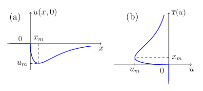
Figure 11: (a) Localized negative initial pulse; (b) the inverse function $\overline{x}(u)$ is represented by two branches $\overline{x}_{1}(u)$ and $\overline{x}_{2}(u)$.

As was shown in Ref. Kamchatnov-19 , we can find velocity of the small-amplitude edge at asymptotically large time for a localized initial pulse by solving Eq. (1) with (6). Then this equation reduces again to Eq. (51), but now it should be solved with the boundary condition

$$\alpha(u_{m})=1$$ (87)

where $u_{m}$ is the maximal value of the velocity in the initial distribution $\widetilde{u}(x)$. The wave number given by Eq. (49) tends here to zero. This gives

$$u=u_{m}-2\ln{\alpha}+\frac{\alpha-1}{\alpha+1}.$$ (88)

At the small-amplitude edge we have $u=0$ and the group velocity (54) plays the role of the left-edge velocity,

$$\frac{1-s_{L}^{1/3}}{1+s_{L}^{1/3}}+\frac{2}{3}\ln{s_{L}}=u_{m}.$$ (89)

Solution of this equation gives asymptotic velocity of small-amplitude edge.

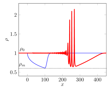
Figure 12: Simple-wave initial state (90) with $\rho_{0}=1$, $x_{0}=100$ and $B=0.05$ is shown by the blue (thin) solid curve. Density profile at $t=300$ is shown by the red (thick) solid curve).

To compare analytical results with numerical calculations, we took the initial state

$$\begin{split}u(x,t=0)=\begin{cases}-A\exp{\left(-\frac{(x-x_{0})^{2}}{4\delta(x_{0}-\delta)}\right)},&\quad\text{if}\quad x\geq\delta,\\ -B\sqrt{x},&\quad\text{if}\quad x<\delta,\end{cases}\end{split}$$ (90)

where

$$A={B}\;\exp{\left(-\frac{1}{4}\left(1-\frac{x_{0}}{\delta}\right)\right)}{\sqrt{\delta}}\;,\quad\delta=x_{0}-0.5.$$

So that density distribution has the form that can be obtained from Eq. (69) (see blue (thin) curve in Fig. 12). The red (thick) curve in Fig. 12 shows the density distribution at $t=300$. Propagation path of the soliton edge is depicted in Fig. 13. Analytical results are shown by a blue (solid) line. As we can see, it agrees reasonably well without any fitting parameter with the result of numerical solution shown by a red dotted line.

The above comparison of the analytical predictions with the numerical solution demonstrates quite convincingly that the method suggested here gives accurate enough description of pulses whose evolution obeys nonintegrable equations.

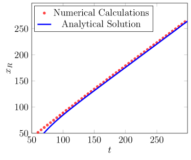
Figure 13: Comparison of the numerical solution of Eqs. (5) (red dots) and the analytical parametric solution (blue (solid) curve) for the soliton edge of DSW. The initial state parameters are indicated in the caption Fig. 12.

V Conclusion

In this paper, we have studied dynamics of ion-sound pulses in plasma for arbitrary form of the initial distribution of simple wave type. This investigation generalizes earlier theories gke-90-plasma ; El-05 applied to the step-like initial conditions only and corresponds to realistic experimental situations ABS-68 ; TBI-70 . Besides that, we derived an asymptotic formula for the number of solitons generated from a localized positive initial pulse. The analytical results obtained here are confirmed by numerical simulations. All that demonstrates that the method of Ref. Kamchatnov-19 is quite effective and can be used for prediction of typical parameters of DSWs generated in real experiments.

- (1) M. G. Forest, C.-J. Rosenberg, and O. C. Wright , On the exact solution for smooth pulses of the defocusing nonlinear Schrödinger modulation equations prior to breaking, Nonlinearity 22, 2287–2308 (2009).
- (2) S. K. Ivanov and A. M. Kamchatnov, Collision of rarefaction waves in Bose-Einstein condensates, Phys. Rev. A 99, 013609 (2019).
- (3) M. Isoard, A. M. Kamchatnov, and N. Pavloff, Wave breaking and formation of dispersive shock waves in a defocusing nonlinear optical material, Phys. Rev. A 99, 053819 (2019).
- (4) M. Isoard, A. M. Kamchatnov, and N. Pavloff, Short-distance propagation of nonlinear optical pulses, in Compte-rendus de la 22-e rencontre du Non Linéaire, Eds. E. Falcon, M. Lefranc, F. Pétrélis, C.-T. Pham, (Non-Linéaire Publications, Saint-Etienne du Rouvray, 2019).
- (5) M. Isoard, A. M. Kamchatnov, and N. Pavloff, Dispersionless evolution of inviscid nonlinear pulses, EPL 129, 64003 (2020).
- (6) A. M. Kamchatnov, Nonlinear Periodic Waves and Their Modulations—An Introductory Course, (World Scientific, Singapore, 2000).
- (7) G. A. El and M. A. Hoefer, Dispersive shock waves and modulation theory, Physica D 333, 15, 11–65 (2016).
- (8) P. M. Bazin, Recherches experimentales sur la propagation des ondes (experimental research on wave propagation), Mem. Pres. Acad. Sci., Paris 19, 495–644 (1865).
- (9) H. P. G. Darcy, H. E. Bazin, Recherches Hydrauliques, Tech. Rep. 1ere et 2eme, Imprimerie Imperiales, Paris, France, 1865.
- (10) T. B. Benjamin and M. J. Lighthill, On cnoidal waves and bores, Proc. R. Soc. London, Ser. A 224, 448–460 (1954).
- (11) N. F. Smyth, P. E. Holloway, Hydraulic jump and undular bore formation on a shelf break, J. Phys. Oceanogr. 18 (7), 947–962 (1988).
- (12) D. R. Christie, The morning glory of the Gulf of Carpentaria: a paradigm for non-linear waves in the lower atmosphere, Austral. Met. Mag. 41, 21–60 (1992).
- (13) M. O. G. Hills, D. R. Durran, Nonstationary trapped lee waves generated by the passage of an isolated jet, J. Atmos. Sci. 69, 3040–3059 (2012).
- (14) Z. Dutton, M. Budde, C. Slowe, and L. V. Hau, Observation of quantum shock waves created with ultra-compressed slow light pulses in a Bose-Einstein condensate, Science 293, 5530, 663–668 (2001).
- (15) T. P. Simula, P. Engels, I. Coddington, V. Schweikhard, E. A. Cornell, and R. J. Ballagh, Observations on Sound Propagation in Rapidly Rotating Bose-Einstein Condensate, Phys. Rev. Lett. 94, 080404 (2005).
- (16) A. M. Kamchatnov, A. Gammal, and R. A. Kraenkel, Dissipationless shock waves in Bose–Einstein condensates with repulsive interaction between atoms, Phys. Rev. A 69, 063605 (2004).
- (17) M. A. Hoefer, M. J. Ablowitz, I. Coddington, E. A. Cornell, P. Engels, and V. Schweikhard, Dispersive and classical shock waves in Bose-Einstein condensates and gas dynamics, Phys. Rev. A 74, 023623 (2006).
- (18) P. A. Praveen Janantha, P. Sprenger, M. A. Hoefer, and M. Wu, Observation of self-cavitating envelope dispersive shock waves in yttrium iron garnet thin films, Phys. Rev. Lett. 119, 024101 (2017).
- (19) Y. C. Mo, R. A. Kishek, D. Feldman, I. Haber, B. Beaudoin, P. G. O’Shea, J. C. T. Thangaraj, Experimental observations of soliton wave trains in electron beams, Phys. Rev. Lett. 110 (8), 084802 (2013).
- (20) J. E. Rothenberg, D. Grischkowsky, Observation of the formation of an optical intensity shock and wave breaking in the nonlinear propagation of pulses in optical fibers, Phys. Rev. Lett. 62 (5), 531 (1989).
- (21) W. Wan, S. Jia, J. W. Fleischer, Dispersive superfluid-like shock waves in nonlinear optics, Nat. Phys. 3 (1) 46–51 (2007).
- (22) Y. Kodama, The Whitham equations for optical communications: mathematical theory of NRZ, SIAM J. Appl. Math. 59 (6), 2162–2192 (1999).
- (23) S. G. Alikhanov, V. G. Belan, and R. Z. Sagdeev, Nonlinear ion-acoustic waves in a plasma, JETP Letters 7, 11, 318–319 (1968) [ZhETF Pis’ma 7, 11, 405–408 (1968)].
- (24) R. J. Taylor, D. R. Baker, and H. Ikezi, Observation of collisionless electrostatic shocks, Phys. Fluids 11, 606 (1970).
- (25) A. V. Gurevich, A. P. Meshcherkin, Expanding self-similar discontinuities and shock waves in dispersive hydrodynamics, Zh. Eksp. Teor. Fiz. 87, 1277–1292 (1984) [Sov. Phys. JETP 60, 732–740 (1984)].
- (26) S. S. Moiseev, R. Z. Sagdeev, Collisionless shock waves in a plasma in a weak magnetic field, J. Nucl. Energy C 5, 43–47 (1963).
- (27) V. Karpman, Non-Linear Waves in Dispersive Media (Elsevier, Amsterdam, 1974).
- (28) Y. Saitou, Y. Nakamura, Ion-acoustic soliton-like waves undergoing Landau damping, Physics Letters A 343, 397–402 (2005).
- (29) L. Romagnani, S. V. Bulanov, M. Borghesi, P. Audebert, J. C. Gauthier, K. Löwenbrück, A. J. Mackinnon, P. Patel, G. Pretzler, T. Toncian, O. Willi, Observation of collisionless shocks in Laser-plasma experiments, Rev. Phys. Lett., 101, 025004 (2008).
- (30) H. Bailung, Y. Nakamura, and Y. Saitou, Observation of ion-acoustic shock wave transition due to enhanced Landau damping, Physics of Plasmas 15, 052311 (2008).
- (31) Y. Nakamura, H. Bailung, and P. K. Shukla, Observation of ion-acoustic shocks in a dusty plasma, Phys. Rev. Lett. 83, 1602 (1999).
- (32) S. I. Popel, A. P. Golub’, T. V. Losseva, Dust ion-acoustic shock-wave structures: theory and laboratory experiments, JETP Lett. 74, 362–366 (2001).
- (33) Y. Nakamura, Experiments on ion-acoustic shock waves in a dusty plasma, Phys. Plasmas 9, 440–445 (2002).
- (34) A. A. Mamun, R. A. Cairns, and P. K. Shukla, Dust negative ion acoustic shock waves in a dusty multi-ion plasma, Phys. Lett. A 373, 27–28, pp. 2355–2359 (2009).
- (35) S. S. Duha, Dust negative ion acoustic shock waves in a dusty multiion plasma with positive dust charging current, Phys. Plasmas 16 (11), 113701 (2009).
- (36) A. V. Gurevich and L. P. Pitaevskii, Nonstationary structure of a collision less shock wave, Zh. Eksp. Teor. Fiz. 65, 590 (1973) [Sov. Phys. JETP 38, 291 (1974)].
- (37) G. B. Whitham, Non-linear dispersive waves, Proc. R. Soc. London, Ser. A 283, 238 (1965).
- (38) G. B. Whitham, Linear and Nonlinear Waves, (Wiley Interscience, New York, 1974).
- (39) H. Washimi and T. Taniuti, Propagation of ion-acoustic solitary waves of small amplitude, Phys. Rev. Lett. 17 (19) 996–998 (1966).
- (40) R. Z. Sagdeev, Cooperative phenomena and shock waves in collisionless plasmas, Rev. Plasma Phys. 4, 23–91 (1966).
- (41) G. Chanteur and M. Raadu, Formation of shocklike modified Korteweg-de Vries solitons: Application to double layers, Phys. Fluids 30 (9), 2708–2719 (1987).
- (42) M. S. Ruderman, T. Talipova, and E. Pelinovsky, Dynamics of modulationally unstable ion-acoustic wavepackets in plasmas with negative ions, J. Plasma Phys. 74 (05), 639–656 (2008).
- (43) V. E. Zakharov, Collapse of Langmuir Waves, Zh. Eksp. Teor. Fiz. 62, 1745–1759 (1972) [Sov. Phys. JETP 35, 908–914 (1972)].
- (44) A. Rogister, Parallel Propagation of Nonlinear Low-Frequency Waves in High- Plasma, Phys. Fluids 14, 2733 (1971).
- (45) E. Mjølhus, On the modulational instability of hydromagnetic waves parallel to the magnetic field, J. Plasma Phys. 16, 321–334 (1976).
- (46) A. V. Gurevich, A. L. Krylov, G. A. El, Nonlinear wave generation in a nonisothermal plasma, Sov. J. Plasma Phys., 16, 248 (1990).
- (47) G. A. El, Resolution of a shock in hyperbolic systems modified by weak dispersion, Chaos 15, 037103 (2005); ibid. 16, 029901 (2006).
- (48) A. M. Kamchatnov, Dispersive shock wave theory for nonintegrable equations, Phys. Rev. E 99, 012203 (2019).
- (49) S. K. Ivanov and A. M. Kamchatnov, Evolution of wave pulses in fully nonlinear shallow-water theory, Physics of Fluids 31, 057102 (2019).
- (50) G. G. Stokes, The Outskirts of the Solitary Wave, in Mathematical and Physical Papers, vol. V, p. 163 (UP, Cambridge, 1905).
- (51) H. Lamb, Hydrodynamics (UP, Campridge, 1994).
- (52) G. A. El, V. V. Khodorovsky, A. V. Tyurina, Determination of boundaries of unsteady oscillatory zone in asymptotic solutions of non-integrable dispersive wave equations, Phys. Lett. A 318, 526–536 (2003).
- (53) R. Z. Sagdeev, Cooperative phenomena and shock waves in collisionless plasmas, in: M.A. Leontovich (Ed.), Reviews of Plasma Physics, vol. 4, Consultants Bureau, New York, 1966.
- (54) L. D. Landau and E. M. Lifshitz, Fluid Mechanics (Pergamon, Oxford) 1987.
- (55) S. P. Tsarev, The geometry of hamiltonian systems of hydrodynamic type. The generalized hodograph method, Mathematics of the USSR-Izvestiya, 37 (2), 397 (1991).
- (56) A. Sommerfeld, Partial Differential Equations in Physics, Academic Press, N. Y., 1949.
- (57) R. Courant and D. Hilbert, Methods of Mathematical Physics, Vol. II, Interscience Publishers, N. Y., 1962.
- (58) B. Riemann, Über die Fortpflanzung ebener Luftwellen von endlicher Schwingungsweite, Abh. Ges. Wiss. Göttingen, Math.-phys. Kl. 8, 43 (1860).
- (59) E. T. Whittaker and D. N. Watson, A Course of Modern Analysis, Cambridge Univ., Cambridge, (1927).
- (60) G. S. S. Ludford, On an extension of Riemann’s method of integration, with applications to one-dimensional gas dynamics, Proc. Cambridge Philos. Soc. 48, 499–510 (1952).
- (61) A. V. Gurevich and L. P. Pitaevskii, Averaged description of waves in the Korteweg-de Vries-Burgers equation, Zh. Eksp. Teor. Fiz., 93, 871 (1987) [Sov. Phys. JETP, 66, 490 (1987)].
- (62) A. M. Kamchatnov, Theory of quasi-simple dispersive shock waves and number of solitons evolved from a nonlinear pulse, preprint arXiv:2008.09786 (2020).
- (63) G. A. El, A. Gammal, E. G. Khamis, R. A. Kraenkel, A. M. Kamchatnov, Theory of optical dispersive shock waves in photorefractive media, Phys. Rev. A 76, 053813 (2007).
- (64) G. A. El, R. H. J. Grimshaw, N. F. Smyth, Asymptotic description of solitary wave trains in fully nonlinear shallow-water theory, Physica D 237, 2423–2435 (2008).