On the Combined Role of Cosmic Rays and Supernova-Driven Turbulence for Galactic Dynamos

Abstract

Large-scale coherent magnetic fields observed in the nearby galaxies are thought to originate by a mean-field dynamo. This is governed via the turbulent electromotive force (EMF, $\overline{\mbox{\boldmath${\cal E}$}{}}$) generated by the helical turbulence driven by supernova (SN) explosions in the differentially rotating interstellar medium (ISM). In this paper we aim to investigate the possibility of dynamo action by the virtue of buoyancy due to a cosmic ray (CR) component injected through the SN explosions. We do this by analysing the magnetohydrodynamic simulations of local shearing box of ISM, in which the turbulence is driven via random SN explosions and the energy of the explosion is distributed in the CR and/or thermal energy components. We use the magnetic field aligned diffusion prescription for the propagation of CR. We compare the evolution of magnetic fields in the models with the CR component to our previous models that did not involve the CR. We demonstrate that the inclusion of CR component enhances the growth of dynamo slightly. We further compute the underlying dynamo coefficients using the test-fields method, and argue that the entire evolution of the large scale mean magnetic field can be reproduced with an $\alpha-\Omega$ dynamo model. We also show that the inclusion of CR component leads to an unbalanced turbulent pumping between magnetic field components and additional dynamo action by the Rädler effect.

1 Introduction

The origin of kilo-parsec scale magnetic fields observed in the nearby galaxies through the polarized radio synchrotron emission (eg. Fletcher, 2010; Beck, 2012, etc.) is attributed to the large scale dynamo operating in the ISM. This is driven mainly via the helical turbulent motions in the interstellar medium, coupled with the differential shear and vertical density stratification. This mechanism, along with some phenomenological approximations about the properties of background turbulence, in principle explains the growth of magnetic fields from small initial strengths to large-scale equipartition strengths against the diffusive losses (Beck et al., 1996; Shukurov, 2005; Beck & Wielebinski, 2013), and the characteristic times it takes for the field to reach the equipatition strength turn out to be of the order of $\sim\,{\rm Gyr}\,$. This is perhaps a much too slow to account for the strong equipartition strength magnetic fields observed in the high redshift galaxies with $z>1$ (eg. Bernet et al., 2008) or even for that in the slowly rotating nearby galaxies. This discrepancy leads one to invoke some additional mechanism such as cosmic rays boosting the typical dynamo action. The idea of CR driven dynamo was initially discussed by Parker (1992), this predicted the possibility of enhanced dynamo action by the virtue of additional CR buoyant instability, that inflates the magnetic field structures (see also Brandenburg, 2018a). Based on the conventional dynamo formulation Parker further suggested a simple model for the flux loss through the gaseous disc due to buoyancy by substituting the transport terms $B_{\phi}/t_{d}$. These terms are supposed to encapsulate the non advective flux transport associated with the buoyant instability, and leads to the fast dynamo action in characteristic field mixing times. Hanasz & Lesch (2000) indirectly verified such a dynamo action via the numerical simulations of rising magnetic flux tubes and found e-folding times of mean field of the order of $100\,{\rm Myr}\,$. Supplementing this Hanasz et al. (2009); Siejkowski et al. (2010); Kulpa-Dybeł et al. (2015); Girichidis et al. (2016) etc. also demonstrated the fast amplification of regular magnetic fields via the direct MHD simulation of global galactic ISM including cosmic ray driven turbulence, along with the differential shear (but excluding the viscous term). To complement this, we aim here to extend our previous analysis of dynamo mechanism in SN driven ISM turbulence Bendre et al. (2015), by including the CR component and investigate the influence of magnetic field dependent propagation of CR on the dynamo. Here we focus on estimating the dynamo coefficients from the direct MHD simulations and effect CR component has on them by comparing with our previous analysis without the CR.

This manuscript is structured as follows: In Sec.  2 we describe our simulation setup with relevant equations, followed by a description of simulated models and parameters in Sec.  3. In Sec.  4 we discuss the overall outcomes of the simulations, estimation of dynamo coefficients and compare the results with that in our previous analysis in Bendre et al. (2015). In Sec.  5 we list out main conclusion, which is followed a summary in Sec.  6.

2 Model Equations

We use the NIRVANA MHD code (Ziegler, 2008) to simulate our system of turbulent ISM in a shearing Cartesian local box of dimensions $0.8\,{\rm kpc}\,\times 0.8\,{\rm kpc}\,$ in $x$ (radial) and $y$ (azimuthal) direction and $-2.13\,{\rm to}\,2.13\,{\rm kpc}\,$ in $z$ (vertical) direction, with galactic midplane situated at $z=0$. We use the shearing periodic boundary conditions in $x$ direction to incorporate the effect of differential shear, along with angular velocity $\Omega$ that scales as $R^{-1}$ (where $R$ is the radius ) with $\Omega=100$ km s^-1 $\,{\rm kpc}\,^{-1}$ at the center of the box, mimicking the flat rotation curve. In the azimuthal $y$ direction we use periodic boundary conditions. While at the $z$ boundaries we allow the gas outflow, by setting the inward velocity components to zero, while for the CR energy we use the gradient condition at the $z$ boundaries. With this setup we solve the following set of differential equations,

$$\frac{\partial\rho}{\partial t}+\nabla\cdot\left(\rho\mathbf{U}\right) = 0\,,$$

$$\frac{\partial\left(\rho\mathbf{U}\right)}{\partial t}+\nabla\cdot\left[\rho\mathbf{UU}+\mathrm{p}^{\star}-\mathbf{BB}\right] = -2\rho\ \Omega\ \hat{z}\times\mathbf{U}$$

$$+2\rho\ \Omega^{2}qx\hat{x}$$

$$+\rho\mathrm{g}\ \hat{z}+\nabla\cdot\tau\,,$$

$$\frac{\partial e}{\partial t}+\nabla\cdot\left[\left(e+\mathrm{p}^{\star}\right)\mathbf{U}-\left(\mathbf{U}\cdot\mathbf{B}\right)\mathbf{B}\right] = +2\rho\ \Omega^{2}qx\ \hat{x}\cdot\mathbf{U}$$

$$+\rho\mathrm{g}\ \hat{z}\cdot\mathbf{U}+\nabla\cdot\tau\mathbf{U}$$

$$+\nabla\cdot\left[\eta\mathbf{B}\times\left(\nabla\times\mathbf{B}\right)\right]$$

$$+\nabla\cdot\kappa\nabla{T}-\rho^{2}\Lambda\left({T}\right)$$

$$+\Gamma_{\mathrm{SN}}+\rho\ \Gamma\left(z\right)\,,$$

$$\frac{\partial\mathbf{B}}{\partial t}-\nabla\times\left(\mathbf{U}\times\mathbf{B}-\eta_{m}\nabla\times\mathbf{B}\right) = 0\,,$$

$$\frac{\partial e_{c}}{\partial t}+\nabla\cdot\left(e_{c}\mathbf{U}+\mathcal{F}_{c}\right) = -\mathrm{p}_{c}\nabla\cdot\mathbf{U}+\mathcal{Q}_{c}\,,$$ (1)

The first four equations in the set represent mass conservation, momentum conservation, total energy conservation and induction equation respectively, similar to Bendre et al. (2015), and all the symbols carry their usual meanings eg. $\rho$, $\mathbf{U}$, $e$ and $\mathbf{B}$ denoting the density, velocity, total energy and magnetic field respectively. The last equation is an addition and it describes the time evolution of CR energy density $e_{c}$. The associated notations used therein namely ${\rm p}^{*}$, ${\rm p}_{c}$ and $Q_{c}$ etc. are defined in the following paragraphs. Here the propagation of CR energy density is modelled using the field aligned diffusion prescription, encapsulated in the anisotropic diffusion for CR energy flux $\nabla\cdot\mathcal{F}_{c}$. We follow the non-Fickian prescription similar to Snodin et al. (2006) to compute this flux term. Specifically we solve the following telegraph equation to obtain the evolution of $\mathcal{F}_{c}$ simultaneously with Eq.  1.

$$\frac{d\mathcal{F}_{ci}}{dt}=\frac{1}{\tau_{c}}\left(K_{ij}\nabla_{j}e_{c}-\mathcal{F}_{ci}\right)$$ (2)

The diffusion coefficient $K_{ij}$ is expressed by

$$K_{ij}=K_{\perp}\delta_{ij}+K_{\parallel}\hat{\mathbf{B}}_{i}\hat{\mathbf{B}}_{j}$$ (3)

where $K_{\perp}$ and $K_{\parallel}$ are diffusion coefficients in perpendicular and parallel to the direction of local magnetic field respectively, and $\hat{\mathbf{B}}_{i}$ and $\hat{\mathbf{B}}_{j}$ are $i$ and $j^{\rm th}$ components of the unit vector in the direction of magnetic field $\hat{\mathbf{B}}=\mathbf{B}/|\mathbf{B}|$.

This non-Fickian prescription of field aligned diffusion of CR energy (Eq.  2) is preferred instead of the standard Fickian one (eg. $\mathcal{F}_{ci}=-K_{ij}\nabla_{j}e_{c}$) in order to restrict the propagation speed of diffusion to the finite values especially in vicinity of magnetic field configuration such as an ‘x’ point (eg. $\mathbf{B}=\left(\sin{\left(\pi x/L_{x}\right)},~{}\sin{\left(-\pi y/L_{y}\right)},~{}0\right)$). This is achieved by choosing a finite value for the correlation time $\tau_{c}$ in Eq.  2. Solution to Eq.  2 approaches to the Fickian diffusion flux, as the estimated value of Strouhal number, $S_{t}=\sqrt{K_{\parallel}\tau_{c}}/h$ (where $h$ is the length scale) approaches zero. For the opposite extreme, when $S_{t}$ attains higher values, solution to Eq.  2 becomes oscillatory. For the models presented in here the value of $S_{t}$ is $\sim 10^{-2}$, and therefore the solution is very similar to the one expected when using the standard Fickian prescription for the CR flux (see eg. Bendre, 2016). In addition to the field aligned diffusion we have also incorporated a small isotropic diffusion term for CR energy, with a diffusion coefficient much smaller than both $K_{\parallel}$ and $K_{\perp}$, this is mainly for the numerical reasons.

Furthermore the term $\nabla\cdot e_{c}\mathbf{U}$ encapsulates the advection of CR energy. An extra pressure term $\mathrm{p}_{c}$ due to CR energy, back reacts on the flow velocity through the Navier-Stokes equation wherein $\mathrm{p}^{\star}$ represents the total pressure, that is thermal pressure, magnetic pressure and CR pressure. First two of these pressure contributions have already been discussed in Bendre et al. (2015) and Bendre (2016), and this extra one is calculated as $\mathrm{p}_{c}=\left(\gamma_{c}-1\right)e_{c}$ (where the used value of $\gamma_{c}=14/9$, similar to Ryu et al. (2003)). Additionally, the term $\mathrm{p}_{c}\nabla\cdot\mathbf{U}$ models the adiabatic heating effect for CR component. Furthermore the term $\mathcal{Q}_{c}$ represents the rate at which CR energy ($e_{c}$) is injected through the SN explosions, which occur randomly at predefined rates. The fraction of SN energy that goes into the ISM as CR and thermal component are chosen as an input parameter.

We also note here that we have not included the effect of CR streaming instability that depends upon the local Alfvén velocity, encapsulating energy transferred from CR to Alfvén waves (see eg. Blandford & Eichler, 1987; Kulsrud, 2005), although the total time for which the model has been run is not sufficient for the magnetic field to reach its equipatition values, and the magnitude of Alfvén velocity is still negligible throughout the run time.

3 Description of Simulated Models

We simulate two models in total, the principle difference in these, lies in the fraction of SN explosion energy that goes into CR and thermal component. To examine the specific effects of CR component on the growth of magnetic field, in one of the models CR, we inject all the SN energy into CR and for the model CR_TH, we inject the same amount of SN energy into a CR component as that in model CR, in addition thermal energy is also injected. Fraction of SN energy going into ISM as a CR and thermal energy ($e_{cr}$ and $e_{th}$) for both of these models, is listed in Table  1. Furthermore the initial conditions for various other parameters (such as mid-plane mass density, vertical scale height etc.) are set so as to mimic the ISM environment in the vicinity of Solar circle in the Milky Way, although the azimuthal angular velocity $\Omega$ for both models is set to $100$ km s^-1 $\,{\rm kpc}\,^{-1}$, faster than that of the Solar circle’s neighbourhood. While the rate of SN explosion in both models is set to $\sim 3\,{\rm kpc}\,^{-2}\,{\rm Myr}\,^{-1}$, about $10\%$ of the SN rate in the Milky Way. Initial configuration of magnetic field is such that $B_{x}$ and $B_{y}$ components have strengths of $-10^{-4}$ $\mu$ G  and $10^{-3}$  $\mu$ G  respectively at the midplane, with scale-heights of $\sim 325\,{\rm pc}\,$ (equivalent to the initial density scale-heights), also the strength of $B_{z}$ component is about $\sim 10^{-3}$  $\mu$ G  , throughout the box with vertical flux of about $0.0064$  $\mu$ G  $\,{\rm kpc}\,^{2}$ threading the $x-y$ plane.

Model	$e_{c}$	$e_{th}$
	$\,{\rm erg}\,$	$\,{\rm erg}\,$
CR	$10^{50}$	$0$
CR_TH	$10^{50}$	$9\times 10^{50}$

Table 1: Distribution of SN explosion energy

For the CR diffusion coefficients we choose $K_{\parallel}=3\times 10^{27}\,{\rm cm}^{2}{\rm s}^{-1}$ and the ratio $K_{\parallel}/K_{\perp}$ of 100. These are at least an order of magnitude smaller than the effective diffusion coefficients expected for  $\mu$ G  strength magnetic fields (eg. Ryu et al., 2003). This is done mainly to constrain the time step and have a sufficiently long simulation in realistic times. Moreover these diffusion coefficients are expected to depend on the CR energy itself, roughly as $K_{\parallel}\propto e_{c}^{-0.3}$, (see eg. Nava & Gabici, 2013), and on the intermittency of the magnetic fields (see eg. Shukurov et al., 2017), both of these effects are not incorporated here. This choice of diffusion coefficients likely impacts the multiphase morphology of ISM. We therefore categorically refrain from analyzing the impact of the inclusion of CR energy on the properties of ISM and the volume filling fractions of various ISM phases etc. in this work and focus mainly on the growth of magnetic field and the properties of dynamo thus realized.

4 Results

To analyze the results of these simulations in the context of dynamo we first define the average/mean of the flow variables ${\mathbf{U}}$ and ${\mathbf{B}}$ by integrating them over the horizontal planes and express the mean quantities as the functions of $z$;

$$\overline{\mathbf{U}}\left(z,t\right) =\frac{1}{L_{x}\,L_{y}}\iint\mathbf{U}\,{\rm d}x{\rm d}y,$$

$$\overline{\mathbf{B}}\left(z,t\right) =\frac{1}{L_{x}\,L_{y}}\iint\mathbf{B}\,{\rm d}x{\rm d}y.$$ (4)

This definition allows one to express the local velocity and magnetic fields as the sums of their respective mean and fluctuating components, $\mathbf{U}=\overline{\mathbf{U}}+\mathbf{u}$ and $\mathbf{B}=\overline{\mathbf{B}}+\mathbf{b}$.

4.1 General Evolution

Within first $\sim 50-100\,{\rm Myr}\,$ kinetic, thermal and CR energy in both models reach a quasi-stationary state, with CR energy being the largest contribution to overall energy budget. This is presumably due to an almost order of magnitude weaker values of diffusion coefficients used in our simulations. The magnitude CR energy in this quasi-stationary state is almost 2-3 times higher in CR_TH, a model that includes the CR and thermal energy as an input from the SN explosions, than in the model CR. This could be attributed to the adiabatic rise (expressed by the term $p_{c}\nabla\cdot\mathbf{U}$ in the CR propagation equation ), due to higher local velocities in model CR_TH. This quasi-stationary state is also associated with emergent steady vertical profiles of mean outward wind velocity $\overline{U}_{z}$ (averaged over $x-y$ plane), these profiles are comparatively flatter in the inner part of the disc $|z|<1\,{\rm kpc}\,$ than in the outer parts where these increase quadratically, at $z=2\,{\rm kpc}\,$, magnitude of $\overline{U}_{z}$ is about $24$ km s^-1 . This increase is more prominent for both models with CR element than that for those which include purely thermally driven SN explosions. From our previous simulations we were able to derive a dependence of the magnitude of $\overline{U}_{z}$ on the rate of SN explosions, the trend goes roughly as $|\overline{U}_{z}|\sim\sigma^{0.4}$, where the $\sigma$ stands for the normalized SN explosions’ rate (similar to Gressel et al., 2013b, referaces therein). Magnitudes of $\overline{U}_{z}$ at the outer boundaries in the CR simulations is almost twice as high compared to its value expected from this SN rate scaling, a difference that could also be attributed to a different vertical hydrodynamic equilibrium due to additional CR pressure. For the model CR_TH on the other hand the inner profiles of $\overline{U}_{z}$ (between approximately $|z|<1\,{\rm kpc}\,$) tend to be similar to the once expected for this SN rate. These vertical profiles of wind are shown in Fig.  1 for both models.

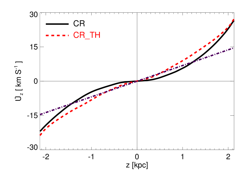
Figure 1: Black solid line shows the stationary vertical profile of outward wind, $\overline{U}_{z}$ in model CR|, while red-dashed line represents the same for model CR_TH|. The dot-dashed line in color blue represents the expected vertical profile of wind for the used value of SN rate here. The SN rate scaling derived from the trend seen in our previous simulations without CR component.

4.2 Evolution of Magnetic Energy

After the initial mixing phase of $\sim 50\,{\rm Myr}\,$, magnetic energy $E_{m}$ in both models amplifies exponentially at e-folding times of approximately 60 and $75\,{\rm Myr}\,$ for models CR and CR_TH, respectively, this time evolution is shown in the left hand panel of Fig.  2 with black solid lines. Overall these growth rates are much faster than that for the purely thermal SN models discussed in Bendre et al. (2015) where the e-folding time was found to be $\sim 100\,{\rm Myr}\,$ irrespective of SN rate. This hints at the enhancement of growth rate of dynamo with inclusion of the CR component. Vertical profiles of mean magnetic field components $\overline{{B}}_{x}$ and $\overline{{B}}_{y}$ in both models amplify exponentially and within $\sim 100\,{\rm Myr}\,$ attain a vertically symmetric profile. For the model CR_TH these vertical profiles are double peaked, with their maximums located at $\sim\pm 200\,{\rm pc}\,$, and the scale height of approximately $\sim 1\,{\rm kpc}\,$. These are also superimposed with comparatively smaller peaks at $\sim\pm 1.2\,{\rm kpc}\,$ with opposite signs than the inner peaks located at $\sim\pm 200\,{\rm pc}\,$. While for the purely CR model CR these vertical profiles are similar to those in CR_TH except the negative peaks are located at $\sim 0.8\,{\rm kpc}\,$ and are much more pronounced. This is seen clearly with black solid lines in the right hand panels of Fig.  2, where we show the vertical profiles of $\overline{B}_{y}$ after $0.6\,{\rm Gyr}\,$ for both models. Overall the mean field profiles are wider in the model CR_TH perhaps due to additional advection present due to thermal energy. However, as a consequence of the lack of advection, in the pure CR model CR mean magnetic field tend to stay longer in the inner dynamo active region. This leads to a slightly faster growth rate of mean-fields on the model CR as shown in the right hand panel of Fig.  2.

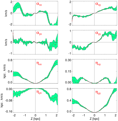
a)       b)

Figure 3: Panel (a) Red dashed lines indicate the vertical profiles of dynamo coefficients for model CR|, along with corresponding $1-\sigma$ error estimates shown in green shaded regions. Panel (b) similar to Panel (a) but for model CR_TH|.

This peculiar shape of $\overline{{B}}_{x}$ and $\overline{{B}}_{y}$ profiles is markedly different from the ones seen in purely thermal SN models, where a vertically symmetric profile with a single peak located at $z=0$ was consistently obtained regardless of the SN explosions rate. Although a similar vertical profiles of mean field have been shown to evolve in another similar setup (see Fig. 3. of Hanasz et al., 2004).

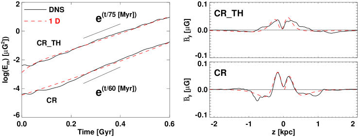
Figure 2: Left Panel Solid-black lines show the amplification of mean magnetic energy in models CR| and CR_TH| shown in logarithemic units. We have multiplied the magnetic energy in model CR_TH| by a constant factor of 2, to avoid the overlap. Overplotted in red dashed lines are the time evolution plots of magnetic energy in respective models calculated using 1-D dynamo equations. Note the overlap of both curves, indicating the a qualitative similarity in the evolution magnetic energy. Right Panel Black-solid lines show the vertical profiles of the azimuthal components of magnetic field after $600\,{\rm Myr}\,$ of evolution for model CR| (bottom panel), and for the model CR_TH| (top panel). Red dashed lines plotted in both panels also show the vertical profiles of $\overline{B}_{y}$ after $600\,{\rm Myr}\,$ in both models but calculated using the 1-D dynamo equations. Note the approximate similarity of these profiles.

4.3 Mean Field Formulation

In these simulations both $\overline{\mathbf{B}}$ and $\mathbf{b}$ amplify exponentially at the e-folding time of $150$ and $120\,{\rm Myr}\,$ approximately, for models CR_TH and CR respectively. In order to understand this amplification and implications of CR component for it, we use the standard mean-field dynamo formulation (Krause & Rädler, 1980), while relying on the definition of mean given in Eq.  4. In the dynamo framework, one seeks to understand the growth of mean magnetic field $\overline{\mathbf{B}}$ for a given background flow $\overline{\mathbf{U}}$ (eg. Moffatt, 1978). By substituting the magnetic and velocity field as a sum of mean and turbulent components in the induction equation, one obtains the induction equation for the mean field, which can be written as

$$\frac{\partial\overline{\mathbf{B}}}{\partial t}=\nabla\times\left(\overline{\mathbf{U}}\times\overline{\mathbf{B}}-\eta_{m}\nabla\times\overline{\mathbf{B}}+\overline{\mbox{\boldmath${\cal E}$}{}}\right)$$ (5)

This is similar to the evolution equation of total magnetic field $\mathbf{B}$ eg. Eq.  1, except for an extra EMF term $\overline{\mbox{\boldmath${\cal E}$}{}}=\overline{\mathbf{u}\times\mathbf{b}}$, which serves as a main driver for the amplification process. By employing the widely used Second Order Correlation Approximation (SOCA) (eg. Rädler, 2014), components of EMF are modeled as linear functional of mean magnetic field and its first derivatives,

$$\overline{\mbox{\boldmath${\cal E}$}{}}_{i}=\alpha_{ij}\overline{B}_{j}-\eta_{ij}\left(\nabla\times\overline{\mathbf{B}}\right)_{j},$$ (6)

where the tensorial quantities $\alpha_{ij}$ and $\eta_{ij}$ represent the dynamo coefficients that depend on the properties of background turbulence. Here the diagonal components of $\alpha_{ij}$ encapsulate the classical ‘alpha’ effect originating from the net helicity of the turbulent motions, while the off-diagonal ones represent the ‘turbulent pumping effect’ arising from the gradient of turbulent intensity. On the other hand $\eta_{ij}$ tensor’s diagonal components represent the turbulent magnetic-diffusivity effect, and off-diagonal ones represent the Rädler effect Rädler (1969) (see also Brandenburg & Subramanian, 2005, for more discussion). These interpretations become clear when Eq.  5 is expressed in its component form as,

$$\frac{\partial\overline{{B}}_{x}}{\partial t} =\frac{\partial}{\partial z}\Bigg{[}-\left(\overline{U}_{z}+\alpha_{yx}\right)\overline{{B}}_{x}-\alpha_{yy}\,\overline{{B}}_{y}+\eta_{yy}\,\frac{\partial\overline{{B}}_{x}}{\partial z}-\eta_{yx}\,\frac{\partial\overline{{B}}_{y}}{\partial z}\Bigg{]}$$

$$\frac{\partial\overline{{B}}_{y}}{\partial t} =\frac{\partial}{\partial z}\Bigg{[}-\left(\overline{U}_{z}-\alpha_{xy}\right)\overline{{B}}_{y}+\alpha_{xx}\,\overline{{B}}_{x}+\eta_{xx}\,\frac{\partial\overline{{B}}_{y}}{\partial z}-\eta_{xy}\,\frac{\partial\overline{{B}}_{x}}{\partial z}\Bigg{]}$$

$$+q\,\Omega\,\overline{{B}}_{x}$$

$$\frac{\partial\overline{{B}}_{z}}{\partial t} =0.$$ (7)

Here the $\alpha_{xy}$ and $\alpha_{yx}$ appear clearly in the advection term involving $\overline{U}_{z}$ while the diagonal $\alpha_{ij}$ and $\eta_{ij}$ appear as the source and diffusive terms respectively.

Advantage of this type of analysis is the ability to self consistently probe which aspect of turbulent motions are contributing to the amplification process, and to understand the manner in which the additional component of CR is affecting the background turbulence and in turn the evolution of mean field. In the following subsection we qualitatively discuss the computed profiles of dynamo coefficients and effects of CR component upon them.

4.4 Dynamo Coefficients

We use the standard test-fields method to extract the components of dynamo tensors $\alpha_{ij}$ and $\eta_{ij}$. We have already used this method for a similar setup, in our previous analysis Bendre et al. (2015), to calculate the dynamo coefficients in the models with purely thermal SN explosions. More details about the test-fields methods implementation and caveats are discussed in Brandenburg (2009, 2018b); Gressel et al. (2008a) etc. Profiles of all such coefficients as functions of $z$, we have thus computed, are shown in the left and right hand panels of Fig.  3 for model CR and CR_TH respectively, along with their corresponding $1-\sigma$ error estimates shown in green color shade. It is manifestly clear from the figures that the diagonal components of $\alpha_{ij}$ are almost 40 - 50% weaker in model CR than in model CR_TH. Quantitatively speaking at $z=1\,{\rm kpc}\,$ $\alpha_{xx}$ is approximately $0.3\pm 0.08$ km s^-1 in model CR while it is $\sim 0.6\pm 0.15$ km s^-1 in model CR_TH, although it is much noisier than other dynamo coefficients. Whereas $\alpha_{yy}$ component is $0.5\pm 0.15$ km s^-1 and $0.8\pm 0.20$ km s^-1 in model CR and CR_TH respectively. Although for both models, the dynamo coefficients are still almost 4-8 times smaller than their expected values estimated from the trends with respect to SN rate, observed in our previous simulations without CR, highlighting the difference between CR and thermal SN turbulence.

Another aspect in which the CR models differ from the previous models without the CR component is the one of off-diagonal components of both $\alpha_{ij}$ and $\eta_{ij}$ tensors. In particular, the antisymmetric contribution from the $\alpha$ tensor tends to be negligible in the CR model, in a sense that magnitude-wise $\alpha_{yx}$ component is negligible compared to $\alpha_{xy}$ implicating an absence of a systematic turbulent pumping effect $\gamma$. This appears in the mean induction equation as $\gamma\times\overline{\mathbf{B}}$, acting as an advective term, roughly in the direction of the gradient of turbulent intensity. For the model CR_TH on the other hand although the $\alpha_{yx}$ is non-negligible, there is only an approximate antisymmetric off-diagonal part, and therefore there exists a systematic pumping. This is in contrast with the outcomes of our previous simulations of SN driven turbulence without the CR component. In those simulations the turbulence driven by the thermal SN explosions led to an anti-symmetrical off diagonal component of $\alpha_{ij}$ tensor (such that $\alpha_{xy}=-\alpha_{yx}$) or a turbulent pumping term that acted against $\overline{\mathbf{U}}_{z}$ preventing the loss of large scale helicity. This subsequently led to the amplification of mean-field. Inclusion of CR component seems to introduce the seen anisotropy in the pumping of $x$ and $y$ components of mean field, whereas with only the thermal energy injected through SN explosions, the mean magnetic field is isotropically pumped in a sense that $x$ and $y$ components are transported via the $\alpha_{yx}$ and $\alpha_{xy}$ respectively, to a same extent. This anisotropy is possibly a result of the difference between the propagation mechanisms of CR and thermal energy, while the former propagates preferentially along the magnetic field lines as prescribed by the field dependent diffusion of $e_{c}$, the later has no such systematic systematic dependence on the direction. The negligible contribution of $\alpha_{yx}$ in model CR also hinders the growth of $x$ component of mean field compared to its $y$ component, as the $\overline{U}_{z}$ overtakes (see eg. Eq.  7, where we write the Eq.  5 in its component form). This effect is less severe in the model CR_TH because of the non-zero $\alpha_{yx}$ acting against the vertical wind. Such anisotropy has implications for the pitch angles of magnetic fields, that is the angle made by magnetic field line with respect to the azimuthal direction (approximately $\tan^{-1}(\overline{B}_{x}/\overline{B}_{y})$). As a consequence, in model CR the calculated values of pitch angles are much smaller compared to that in model CR_TH. This is markedly different than our previous results without the CR where with the increasing SN rate, outward wind helped saturate the mean magnetic fields to the strengths insufficient to quench the dynamo coefficients and therefore retained the pitch angles even in the saturated phase of magnetic fields.

To further cite the differences in the dynamo coefficients, we refer to the components of $\eta_{ij}$ tensor. It appears that shapes and trends of the vertical profiles are qualitatively similar in both models, and for the diagonal components even their strengths are similar. The off-diagonal components however are twice as strong in model CR_TH than in model CR. Comparative contribution of the diagonal to off-diagonal elements is also much higher than in our previous simulations described in Bendre et al. (2015). The ratios of diagonal to off-diagonal components were found to be at most 10, in our previous simulations irrespective of the SN rates, in fact within the standard $1-\sigma$ error intervals both $\eta_{xy}$ and $\eta_{yx}$ were consistent with zero. However for both models with the CR this ratio is about 2 to 5. The values diagonal $\eta_{ij}$s calculated for both CR and CR_TH using the test-fields method are almost 3-6 times weaker than their expected magnitude extrapolated from the dependence of $\eta_{ij}$ components on the rate of SN explosions derived in Bendre et al. (2015) for the models without the CR component. However both $\eta_{xy}$ and $\eta_{yx}$ turn out to have the expected magnitudes; more or less from the same trend, although it should be noted that in the said previous simulations the off-diagonal $\eta$ coefficients were much noisier. Consequently the estimated value of dynamo number is $\sim 190$ for both CR models as opposed to $\sim 110$ for the models without the CR component.

Remarkably, and contrary to the models without the CR, signs of the $\eta_{yx}$ and $\eta_{xy}$ components very consistently turn out to be negative and positive respectively, in both models with the CR component, which in combination with the differential rotation and shear is shown to lead to the Rädler effect and amplify the mean fields without any systematic $\alpha$ effect. For both models with CR, this effect enhances the growth rate of dynamo by $\sim 17$ to $30\%$, as discussed in the following section.

4.5 Evolution of Mean-Field

To understand the entire evolution of mean magnetic field in both models we simultaneously solve Eq.  7 for $\overline{B}_{x}$ and $\overline{B}_{y}$. The component $\overline{B}_{z}$ does not evolve in time as a consequence of the solenoidity constraint along with the boundary conditions for magnetic field. As an input we choose the vertical profiles of dynamo coefficients calculated using the test-fields method discussed in the previous subsection, and the profile of vertical wind also from the direct simulations. With this setup we solve Eq.  7 using an algorithm based on finite difference method over a staggered grid of size $N_{z}=512$. For boundary conditions we use the continuous gradient condition equivalent to the direct simulations. This is very similar to our previous analysis without the CR component, effect of this additional CR element is captured wholly in the dynamo coefficients and the vertical wind profiles.

It turns out in this analysis that the evolution of mean field predicted using Eq.  7 and dynamo coefficients is largely consistent with what obtains in the direct simulations, for both models. Which seem to show that the dynamo coefficients calculated in the previous subsection do capture the underlying dynamics of the turbulence, and the differences marked in the various dynamo coefficients as discussed above also encapsulate the actual impact of CR component on the evolution of mean magnetic field. In the left and right hand columns of Fig.  4 we compare the contours of time evolution of the vertical profiles of the $y$ component of mean field for models CR and CR_TH respectively, calculated from the DNS and 1-D dynamo models. Note the remarkable similarity in the coloured contours shown in top and bottom panels which use the same color codes. Furthermore the time evolution of mean magnetic energy is also comparable in both DNS and 1-D simulations, eg. in the left hand panel of Fig.  2, black solid lines (showing the evolution of mean magnetic energy in DNS) are comparable to the red-dashed ones showing the evolution magnetic energy in 1-D dynamo simulations. Also in the right hand panels we compare the vertical profiles of azimuthal mean field component at $t=600\,{\rm Myr}\,$, black solid lines show the results from DNS and red-dashed lines are the ones from 1-D dynamo simulations. There is an overall similarity in the evolution of mean field in both types of simulations and it can therefore be safely argued that the computed dynamo coefficients effectively characterize the turbulence that drives the dynamo.

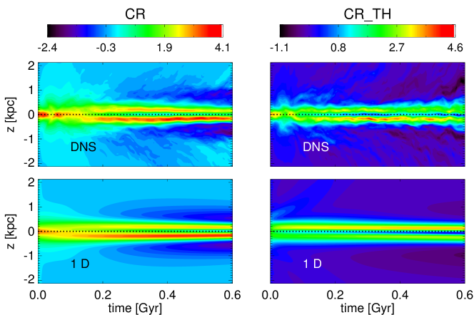
Figure 4: Left column: shows the time evolution of the vertical profiles of the $y$ component of mean magnetic field seen in the direct simulations of model CR| (top panel) while the bottom panel shows the same for the corresponding 1D dynamo model using the dynamo coefficients obtained for the model CR| using the test-fields method. Colour code used for producing these contours is defined in the colourbar at the top, however we have scaled it temporally; by a factor of $\exp{(t/120{\rm\,Myr})}$ to compensate for the exponential growth of the mean magnetic field. Right Column indicated the same as the left column but for the model CR_TH|. Note the qualitative similarity in the evolution of magnetic field in both panels.

Additionally, to identify the impact of non-negligible off-diagonal $\eta$ components on the evolution, we set the corresponding terms in Eq.  7 to zero and run the 1-D simulations with rest of the dynamo coefficients for both CR models. Outcomes of these simulations reveal that the slightly fastened growth rate of dynamo in CR and CR_TH is indeed a result of Rädler effect. This can be seen from Fig.  5 where in left and right hand panels we compare the evolution of mean magnetic energy in models CR and CR_TH respectively. With black dotted lines we show the mean magnetic energy from DNS, along with its counterpart from 1-D dynamo simulations in light-blue solid lines while the red dashed lines show the evolution of the same 1-D dynamo without the off-diagonal $\eta_{ij}$ components. We point out here a clear hindrance in the growth of the dynamo when $\eta_{xy}$ and $\eta_{yx}$ are absent in the simulations. For the model CR the absence of off-diagonal terms translates to almost a $17\%$ decline in the growth rate of mean magnetic energy (e-folding time of $60\,{\rm Myr}\,$ for the model including $\eta_{xy}$ and $\eta_{yx}$ as opposed $70\,{\rm Myr}\,$ without them). Similarly for the model CR_TH the e-folding time increases from $75\,{\rm Myr}\,$ to $100\,{\rm Myr}\,$ once the off-diagonal $\eta$ components are switched-off as can be clearly seen in right panel. Interestingly, even in the absence of systematic $\alpha$ effect, this combination of off-diagonal $\eta$ components and the differential shear is sufficient for the exponential growth of dynamo in both models, as shown by the blue dot-dashed lines. This points towards the Rädler effect dynamo associated with CR turbulence.

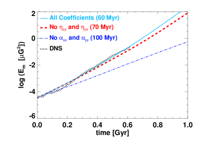
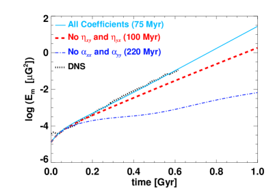
Figure 5: Left Panel shows the time evolution of mean magnetic energy in model CR|. Black dotted line shows the outcome of DNS while the light blue solid line shows the same for corresponding 1 D dynamo model. Red dashed line shows the evolution of mean magnetic energy in a dynamo model where the off-diagonal elements of $\eta$ tensors have been set to zero. The blue dot-dashed line shows a complementary case where the diagonal $\alpha$ elements are turned off and the full $\eta$ tensor is used, highlighting that Rädler effect independently leads to a growing mean field. Approximate e-folding times of magnetic energy in each of the cases are written in brackets. Right Panel is same as the Left panel but for the model CR_TH|. Note that without the $\eta_{xy}$ and $\eta_{yx}$ terms the growth of dynamo is hindered noticeably.

Furthermore to investigate the vertical profiles of $\overline{U}_{z}$ that are dissimilar to the ones seen in the models without the CR, as a potential reason for the enhanced dynamo action, we do a similar exercise. We set the wind term in Eq.  7 to zero and perform 1-D dynamo simulations again. This however reveals that the growth rate of dynamo is not significantly impacted by the wind profiles, the difference however, is that without the outward wind mean magnetic field is concentrated mostly in the inner disc part $\left(-1\,{\rm kpc}\,<z<1\,{\rm kpc}\,\right)$ although with a smaller dynamo time-period.

5 Conclusions

Main effects of CR on the ISM turbulence and mean field dynamo seen in our simulations are as follows,

1. Faster increasing velocities of the outward wind with height.

2. Anisotropy of turbulence transport, which gets reflected in the vertical profiles of off-diagonal $\alpha$ coefficients.

3. Appearance of a Rädler term, which slightly increases the growth rate of mean magnetic field.

4. Slightly enhanced growth of the dynamo with inclusion of CR term.

6 Summary

We have examined here the impact of the field aligned diffusion of CR energy injected through the SN explosions on the evolution of galactic dynamo. We have done so by comparing the evolution of magnetic fields in the model where only thermal energy was injected by SN explosions, to a model that treats the SN explosions as localised injection of both thermal energy and the CR energy. We treat the CR energy as a fluid diffusing in the direction of local magnetic field. We have also compared the general evolution of both models to our previous analysis in which we had studied the dependence of dynamo action on the rate of SN explosions. We have relied upon the standard test-fields method to compute the dynamo coefficients in both models and simulated a simple 1-D dynamo model to examine the effect of various turbulent transport parameters on the inclusion of CR energy and growth of mean magnetic field. We have compared this with our previous analysis of models that do not involve the CR component, however for the current work we have restricted the analysis to the initial kinematic growth phase of the magnetic field.

One of the principle distinctions in the models that involved the CR was the faster growth rates of the mean magnetic fields, compared to models with no CR component. It was also found that for a model that involved SN explosions with purely a CR energy injected in the ISM, the magnetic energy had a slightly faster growth rate compared to the model that includes SN with CR and thermal energy. Inclusion of CR was found also to have a distinctive impact on the off-diagonal elements of the $\alpha$ tensor. Specifically for a model which included only the CR, the magnitude of $\alpha_{yx}$ was found to be negligible compared to that of $\alpha_{xy}$. On the other hand the models that include the SN that expel both CR and thermal energy, $\alpha_{yx}$ was not negligible although smaller than $\alpha_{xy}$. This is in contrast with the purely thermal SN models that we had simulated earlier (Bendre et al., 2015), where $\alpha_{xy}$ and $\alpha_{yx}$ were found to be statistically equal in magnitude but with opposite directions. This resulted into a systematic turbulent pumping (or $\gamma$) effect. The presence of $\gamma$ effect, is a robust result which has been seen in other previous ISM simulations as well Gressel et al. (2008b). The $\gamma$ effect arises as an advection in the direction of the gradient of turbulent intensity, which in the case of galaxies is towards the galactic midplane. Turbulent pumping effect therefore acts essentially in opposition to the advection governed by the outward wind. For the models including the CR component however this effect turned out to be nonuniform for $x$ and $y$ components of the mean magnetic field, implying the more effective outward transport of the $x$ component of the mean magnetic field compared to the $y$. Anisotropy of turbulent pumping is more pronounced in the purely CR model CR than in model CR_TH, where the isotropically propagating thermal energy is possibly introducing a non vanishing $\alpha_{yx}$ (as opposed to CR energy which diffuses preferentially along the mean magnetic field lines). As a consequence the pitch angles seen in model CR are negligible compared to the ones seen in model CR_TH.

Another important distinction in both models involving the CR component is the non-negligible contribution of the off-diagonal component of $\eta$ tensor, $\eta_{xy}$ and $\eta_{yx}$, compared to that in models which do not involve the CR. Resulting into a transverse diffusive transport of the mean magnetic flux. Furthermore it also turned out in both of these models that the components $\eta_{yx}$ and $\eta_{xy}$ were manifestly negative and positive respectively. This is striking, specifically because the component $\eta_{yx}$ in combination with rotation and shear term allows a growing solution to the dynamo equations, depending on the sign of shearing term, via the Rädler effect. This can be elaborated from Eq.  7, where negative sign of $\eta_{yx}$ in the first equation along with $q\,\Omega\overline{B}_{x}$ term in second equation allows the growth of $\overline{\mathbf{B}}$ components, even in the absence of other source terms arising from turbulent helicity i.e. $\alpha_{ij}$. This effect was consistently absent in the models without the CR component, where both $\eta_{xy}$ and $\eta_{yx}$ were approximately zero within $1-\sigma$ confidence interval, even irrespective of the SN explosion rates. However, it should be noted here that the contribution from shear related higher order effects in the expansion of turbulent diffusivity tensor, such as the shear-current effect $\kappa$ (eg. Rogachevskii & Kleeorin, 2003; Brandenburg et al., 2008) also gets added to the off-diagonal terms of $\eta$ tensor mixing up with the contributions arising from $\delta\times\overline{\mathbf{J}}$ effect described by Rädler (1969), where the $\delta$ is an expansion coefficient and $\overline{\mathbf{J}}$ is the mean current (see also the Section 4.4.3 of Rincon, 2019). It appears impossible to disentangle the individual contributions from the available data of the simulations. The presence of Rädler effect may be relevant in explaining the enhanced growth rate of mean field expected for the dynamo operating in turbulence driven by the CR (see eg. Fig.  5), especially given the fact that this effect does not vanish even within the model that involves both CR and thermal energy inputs from SN explosions.

It however still remains to be seen, how these results scale with the magnetic field aligned diffusion coefficients of CR energy, which we plan to address in the future. Nevertheless the computed sets of dynamo tensors reproduce the entire evolution of mean magnetic field seen in the DNS, using 1-D dynamo simulations as can be seen from Fig.  2 and Fig.  4. It would also be of our interest to analyze the saturation mechanism of such a dynamo where CRs are included, and to see how the mean field quenches the dynamo coefficients, similar to Gressel et al. (2013a) for the simulations without the CR. Another open question which we have not analyzed here is the one of how the CR component affects the multiphase structure of ISM, and how and whether they differ characteristically from that in the simulations of ISM without the CRs (eg. Gressel et al., 2008a). It should however be noted here that this prescription may not completely describe the CR propagation in the ISM when dynamical strength magnetic fields exist, and gives rise to a CR streaming instability. Wherein the CR component interacts with Alfvén waves that are generated by itself, this further limits its propagation speed. This effect will probably be important in the dynamical phase.

7 Data Availability

The data underlying this article are available in the repository "On the Combined Role of Cosmic Rays and Supernova-Driven Turbulence for Galactic Dynamos", at Bendre (2020)

References

- Beck (2012) Beck R., 2012, Space Science Reviews, 166, 215
- Beck & Wielebinski (2013) Beck R., Wielebinski R., 2013, Magnetic Fields in Galaxies. Springer Berlin Heidelberg, p. 641, doi:10.1007/978-94-007-5612-0_13
- Beck et al. (1996) Beck R., Brandenburg A., Moss D., Shukurov A., Sokoloff D., 1996, Annual Review of Astronomy and Astrophysics, 34, 155
- Bendre (2016) Bendre A. B., 2016, doctoralthesis, Universität Potsdam
- Bendre (2020) Bendre A. B., 2020, On the Combined Role of Cosmic Rays and Supernova-Driven Turbulence for Galactic Dynamos, doi:10.5281/zenodo.3992802, https://doi.org/10.5281/zenodo.3992802
- Bendre et al. (2015) Bendre A., Gressel O., Elstner D., 2015, Astronomische Nachrichten, 336, 991
- Bernet et al. (2008) Bernet M. L., Miniati F., Lilly S. J., Kronberg P. P., Dessauges-Zavadsky M., 2008, Nature, 454, 302
- Blandford & Eichler (1987) Blandford R., Eichler D., 1987, Phys. Rep., 154, 1
- Brandenburg (2009) Brandenburg A., 2009, Space Science Reviews, 144, 87
- Brandenburg (2018a) Brandenburg A., 2018a, Journal of Plasma Physics, 84, 735840404
- Brandenburg (2018b) Brandenburg A., 2018b, Journal of Plasma Physics, 84, 735840404
- Brandenburg & Subramanian (2005) Brandenburg A., Subramanian K., 2005, Physics Reports, 417, 1
- Brandenburg et al. (2008) Brandenburg A., Rädler K. H., Rheinhardt M., Käpylä P. J., 2008, ApJ, 676, 740
- Fletcher (2010) Fletcher A., 2010, in Kothes R., Landecker T. L., Willis A. G., eds, Astronomical Society of the Pacific Conference Series Vol. 438, The Dynamic Interstellar Medium: A Celebration of the Canadian Galactic Plane Survey. p. 197 (arXiv:1104.2427)
- Girichidis et al. (2016) Girichidis P., et al., 2016, ApJ, 816, L19
- Gressel et al. (2008a) Gressel O., Ziegler U., Elstner D., Rüdiger G., 2008a, Astronomische Nachrichten, 329, 619
- Gressel et al. (2008b) Gressel O., Elstner D., Ziegler U., Rüdiger G., 2008b, A&A, 486, L35
- Gressel et al. (2013a) Gressel O., Bendre A., Elstner D., 2013a, MNRAS, 429, 967
- Gressel et al. (2013b) Gressel O., Elstner D., Ziegler U., 2013b, A&A, 560, A93
- Hanasz & Lesch (2000) Hanasz M., Lesch H., 2000, ApJ, 543, 235
- Hanasz et al. (2004) Hanasz M., Kowal G., Otmianowska-Mazur K., Lesch H., 2004, ApJ, 605, L33
- Hanasz et al. (2009) Hanasz M., Wóltański D., Kowalik K., 2009, ApJ, 706, L155
- Krause & Rädler (1980) Krause F., Rädler K. H., 1980, Mean-field magnetohydrodynamics and dynamo theory
- Kulpa-Dybeł et al. (2015) Kulpa-Dybeł K., Nowak N., Otmianowska-Mazur K., Hanasz M., Siejkowski H., Kulesza-Żydzik B., 2015, A&A, 575, A93
- Kulsrud (2005) Kulsrud R. M., 2005, Plasma physics for astrophysics. Princeton University Press
- Moffatt (1978) Moffatt H. K., 1978, Magnetic Field Generation in Electrically Conducting Fluids. Cambridge University Press, Cambridge
- Nava & Gabici (2013) Nava L., Gabici S., 2013, MNRAS, 429, 1643
- Parker (1992) Parker E. N., 1992, ApJ, 401, 137
- Rädler (1969) Rädler K. H., 1969, Monats. Dt. Akad. Wiss, 11, 272
- Rädler (2014) Rädler K. H., 2014, arXiv e-prints, p. arXiv:1402.6557
- Rincon (2019) Rincon F., 2019, Journal of Plasma Physics, 85, 205850401
- Rogachevskii & Kleeorin (2003) Rogachevskii I., Kleeorin N., 2003, Phys. Rev. E, 68, 036301
- Ryu et al. (2003) Ryu D., Kim J., Hong S. S., Jones T. W., 2003, ApJ, 589, 338
- Shukurov (2005) Shukurov A., 2005, Mesoscale Magnetic Structures in Spiral Galaxies. Springer Berlin Heidelberg, Berlin, Heidelberg, pp 113–135, doi:10.1007/3540313966_6, https://doi.org/10.1007/3540313966_6
- Shukurov et al. (2017) Shukurov A., Snodin A. P., Seta A., Bushby P. J., Wood T. S., 2017, ApJ, 839, L16
- Siejkowski et al. (2010) Siejkowski H., Soida M., Otmianowska-Mazur K., Hanasz M., Bomans D. J., 2010, A&A, 510, A97
- Snodin et al. (2006) Snodin A. P., Brandenburg A., Mee A. J., Shukurov A., 2006, MNRAS, 373, 643
- Ziegler (2008) Ziegler U., 2008, Computer Physics Communications, 179, 227