Calibration of Elastoplastic Constitutive Model Parameters from Full-field Data with Automatic Differentiation-based Sensitivities

Abstract

We present a framework for calibration of parameters in elastoplastic constitutive models that is based on the use of automatic differentiation (AD). The model calibration problem is posed as a partial differential equation-constrained optimization problem where a finite element (FE) model of the coupled equilibrium equation and constitutive model evolution equations serves as the constraint. The objective function quantifies the mismatch between the displacement predicted by the FE model and full-field digital image correlation data, and the optimization problem is solved using gradient-based optimization algorithms. Forward and adjoint sensitivities are used to compute the gradient at considerably less cost than its calculation from finite difference approximations. Through the use of AD, we need only to write the constraints in terms of AD objects, where all of the derivatives required for the forward and inverse problems are obtained by appropriately seeding and evaluating these quantities. We present three numerical examples that verify the correctness of the gradient, demonstrate the AD approach’s parallel computation capabilities via application to a large-scale FE model, and highlight the formulation’s ease of extensibility to other classes of constitutive models.

1 Introduction

Many scenarios of interest in science and engineering involve large, permanent deformations (e.g. vehicle crashes and metal forming). In continuum mechanics the finite deformation theory of plasticity enjoys an increased range of applicability over infinitesimal strain formulations, but its mathematical theory as well as computational implementation through finite elements is more challenging. The field of computational plasticity has matured and computing power has increased to the point that finite deformation elastoplastic models are used in industry, government, and academic labs, although their efficient implementation on high-performance computing (HPC) platforms remains an active area of research.

In order for such models to provide credible predictions, the parameters in the constitutive models must be determined through a calibration procedure which amounts to formulating and solving an inverse problem. In a typical calibration experiment, a sample is deformed in a controlled manner and the deformation and resultant loads are measured. These measurements are then used to inform calibration of an analytical or computational model of the material under study. Traditionally, specialized test specimens such as dogbones for metals described by elastoplastic constitutive models have been used because their geometry justifies the use of assumptions that simplify the mathematical modeling. Namely, prior to necking, the stress and strain are uniaxial and constant in the gauge section, and can be calculated analytically given the applied force and cross-section area (stress) and an extensometer and initial gauge length (strain). While these assumptions facilitate the calibration procedure, they can also increase the number of mechanical tests required to produce an adequate amount of data for accurate calibration. For example, calibration of viscoplastic constitutive models using dogbone specimens requires the execution of multiple tests at constant and distinct strain rates and/or temperatures.

The maturity and relative ease of application of digital image correlation (DIC) provides opportunities to advance beyond traditional test specimens and their associated assumptions [37, 98, 38]. In a typical test, hundreds of optical images of a patterned surface of the sample are acquired. The DIC algorithm then produces a full-field (i.e. densely distributed over the DIC region-of-interest) point cloud of displacement measurements, which can contain tens to hundreds of thousands of points depending on camera resolution and user-defined DIC settings. Furthermore, the typical amount of noise in present in one of these point measurements is on the order of $0.01-0.05$ pixels [85]. The conversion from image to physical units depends on the resolution of the camera and physical dimensions of the field-of-view, but for a well-controlled measurement in a laboratory setting the noise floor in physical units can readily be sub-micron. In fact, the quality of the displacement measurements are so good that one of the primary uses of DIC is to provide experimental data for validation of computational finite element (FE) models, i.e. the DIC measurements are treated as a ground truth.

Digital volume correlation (DVC), the three-dimensional extension of DIC, is being actively developed although its use in constitutive model calibration is less mature [12, 17]. It has the advantage of providing displacements through a sample volume, but in contrast to DIC, it is often difficult or impossible to create an artificial pattern in the sample interior, especially without modifying the base material properties. Therefore, in most cases the microstructure itself serves as the pattern, which is typically not optimal for DVC algorithms [11, 21]. Further, the method of producing images must be capable of penetrating a volume, so imaging systems based on X-rays are commonly used. We do not consider calibration from DVC data in this paper, but extending our computational formulation to volumetric displacement data would be trivial.

As we will discuss shortly, the experimental mechanics community that developed DIC has led the way in using DIC data to calibrate constitutive models, and the most common means of doing so is through an optimization formulation that minimizes the difference between experimental measurements (e.g. DIC data and load) and FE model predictions. It is challenging, however, to fully capitalize on the rich deformation data provided by DIC, as the FE model has to have sufficient fidelity to accurately approximate the motion of the specimen (i.e. to control discretization error in the model) and represent the DIC data in regions of rapid variation. The optimization approaches favored in the literature (genetic algorithms and gradient-based methods that rely on finite difference approximations) require many solutions of the FE model (easily hundreds to thousands), which places a practical limit on the cost and ultimately fidelity of the model, to the point where the high-resolution DIC data is often down-sampled to a considerably coarser FE mesh.

In this paper we present a proof of concept for calibration of parameters in large-scale, finite deformation elastoplastic constitutive models from full-field deformation data using a deterministic partial differential equation (PDE)-constrained optimization formulation where the gradient of the objective function is obtained through forward and adjoint sensitivity analyses. Following [68, 50, 7], we write the constraint equations as coupled residuals, i.e. discretized weak forms for the global equilibrium PDE and local constitutive model evolution equations. A defining feature of our approach is the use of automatic differentiation (AD) to facilitate the computation of the many derivatives present in the formulation.

Automatic differentiation is a technique to computationally evaluate analytic derivatives (to machine precision) of a given function. In the context of PDE-constrained optimization, AD provides the ability to compute various required sensitivities based on implementations of the residuals (and objective function when its derivatives cannot be easily determined), without requiring manual derivative calculations. These sensitivities include the derivatives of these quantities with respect to state variables (e.g. displacement, equivalent plastic strain) and constitutive model parameters. In particular, our approach utilizes forward mode AD to obtain derivative quantities at the element level. Utilizing AD in this manner facilitates the parallelization of required computations [78, 79]. For more details on AD, we refer readers to the canonical book [34]. Our computational implementation uses the C++ operator-overloading AD software package Sacado [80].

After presenting the formulation of the inverse problem, we provide three numerical calibration examples with synthetic DIC data and note that several algorithmic refinements would be required to make our framework suitable for calibration with experimental full-field data. The framework described in this paper, however, is amenable to such extensions. We also remark that our use of AD makes the implementation of other types of constitutive models (e.g. viscoplastic, kinematic hardening, damage) easier than in traditional approaches. Additionally, the model calibration problem shares many similarities to optimal design problems studied in the computational mechanics literature such that this work may be useful in those fields as well.

In the remainder of the introduction, we review existing approaches to elastoplastic model calibration from full-field data and discuss how our work relates to studies in the PDE-constrained optimization and computational plasticity literature that address finite deformation constitutive models.

1.1 Constitutive Model Calibration for Elastoplastic Materials from Full-field Data

The two primary approaches in the experimental mechanics community for calibration from full-field DIC data are known as finite element model updating (FEMU) [9] and the virtual fields method (VFM) [33, 81]. In the VFM, the objective function is a squared mismatch between internal and external virtual work or power instead of measured and predicted displacement or strain subject to PDE constraints. We will not discuss VFM further, save to say it has been used to calibrate parameters in finite deformation elastoplastic constitutive models [87, 49, 88, 43, 42, 66, 65].

In FEMU, an objective function that quantifies the weighted mismatch between model predictions and corresponding experimentally-measured quantities of interest is minimized by iteratively updating the parameters of a FE model using an optimization algorithm. A basic objective function contains data from load-displacement curves, but more sophisticated objective functions employ full-field displacements or strains obtained from DIC. The formulation presented in this paper could be viewed as a FEMU method, the defining difference being that in the FEMU literature finite differences are used to compute the gradient of the objective function or derivatives of the displacement field with respect to the model parameters. This approach to differentiation allows the FE model to be treated in a black-box fashion and thus encourages the use of off-the-shelf software. We avoid the use of finite difference approximations in our work and instead employ forward and adjoint sensitivity analyses. While these techniques require intrusive, non-standard modifications of the FE solver, they are significantly more computationally efficient, as we will demonstrate in this work.

Integrated DIC [84, 67, 75, 90, 73, 15, 74, 72] and DVC [36, 18] approaches that combine the displacement and constitutive model parameter estimation problems have been thoroughly investigated in the literature. In these formulations the objective function is the same one used in standard DIC, a least-squares formulation based on the optical residual that quantifies the mismatch between a reference and deformed image warped by the DIC displacement estimates. The FE model is introduced as a constraint, and most approaches use a Gauss-Newton algorithm to solve the minimization problem. This method requires the computation of displacement sensitivity matrices, and these are also typically obtained using finite differences. Integrated DIC often makes use of global DIC methods, where a FE basis is used to represent the displacement field, and it is often the case that the same basis is used for the FE model and DIC displacements, although this isn’t strictly necessary.

A notable drawback of the reliance on finite difference approximations is the introduction of scaling with dimension of the parameter space. A full nonlinear FE solve is needed to compute each component of the gradient through a forward finite difference approximation. This limitation restricts the practical size of the parameter space, such that most studies consider homogeneous materials described by a single constitutive model with 5-10 parameters. This scaling can also reduce the ability of the FE model to take full advantage of the high temporal and spatial fidelity of the DIC data when cost of solving the FE model on a “fine-enough” mesh is prohibitive.

Finally, due to the expense of the finite deformation elastoplastic FE models and high-dimensional nature of DIC data (spatial and temporal), Bayesian approaches to parameter calibration, where probability distributions for the parameters are obtained, are to date relatively rare. Deterministic calibration, where point estimates of the most likely values of the parameters are calculated given the experimental data, is more common. We do not consider Bayesian inverse formulations in this work, but the computationally-efficient gradient calculation methods we describe could be useful for the construction of surrogate models for emulator-based Bayesian inference and Markov-chain Monte Carlo algorithms that can take advantage of this information.

1.2 PDE-constrained Optimization in Finite Deformation Plasticity

We now turn to the studies of PDE-constrained optimization in the computational mechanics literature where forward and adjoint sensitivity analyses have been applied to finite deformation elastoplastic constitutive models for the purposes of model calibration and optimal design. Each of these articles invariably contains pages of analytic expressions for the derivatives (or related intermediate quantities) that we obtain through the application of AD to element-level residuals.

Parameter identification for finite deformation elastoplastic constitutive models using a principal space formulation has been presented in [63, 60, 61, 62]. The gradient is analytically derived for the continuous form of the governing equations and then discretized (an optimize-then-discretize approach). The numerical results in these studies focus on tensile specimens with measurements of displacement and load, and the objective function quantities the mismatch of point measurements of displacement that are either randomly chosen over a subset of the mesh or located in the necking region.

Numerical formulations for finite deformation plasticity with applications to metal-forming [10, 93, 107, 94, 27, 28, 108, 2] and optimal design of multiscale materials [1, 30, 29, 97, 95, 96] have also been developed using an optimize-then-discretize approach based on forward sensitivity analysis. Notably, many of these formulations incorporate additional constraints such as contact or thermal physics and analytically derive the coupled linear systems used to compute the sensitivities needed for gradient evaluation.

In topology optimization the goal is to produce a structural design that satisfies an optimality criterion [91, 58] given a volume constraint. Earlier studies focused on linear elastic models and minimum compliance formulations, but today authors consider elastoplastic constitutive models and other objective functions such as those that quantify energy dissipation. In topology optimization the design variable is typically a density field that has been “filtered” to produce $0$ or $1$ values (i.e. present or not present) within a given element.

Various authors have considered topology optimization problems for small-strain plasticity [71, 105, 109, 54, 55, 8, 3, 53, 7, 56, 5], but only a few have addressed finite deformation plasticity [104, 40, 4, 6, 41]. We also note that 3D numerical examples are not present in the latter, presumably due to the computational expense and complexity of implementation of these formulations.

Like model calibration, topology optimization is formulated as a PDE-constrained optimization problem. The governing equations can be the same as in our approach, but the objective function is not. The optimization algorithm known as the method of moving asymptotes (MMA) [99] is often used to solve these problems, and a detailed description of this algorithm is not relevant to our work. What is important to mention is that the MMA requires the derivative of the objective function with respect to the design parameters, and in this paper we provide an AD-based recipe for computing this quantity using forward or adjoint sensitivities. In topology optimization most authors use an adjoint-based approach to gradient calculation because the design variable is a heterogeneous material density and therefore is directly related to mesh size such that the dimension of the parameter space makes adjoint approaches the only viable option.

More specifically, most authors follow the adjoint-based approach described in [68] to compute the gradient of the objective function, which was originally presented in the general context of transient coupled nonlinear systems. More recently, [7] presented a unification of this framework for topology optimization of path-dependent materials that shares both the global-local split of the governing equations and discretize-then-optimize strategy followed in our work.

While AD makes a few appearances in the topology optimization literature, to date it has seen more application in fluid mechanics [86, 70, 25, 24]. Its use in solid mechanics is limited to 1D wave propagation [76] and more recently fluid-structure interaction [31].

Lastly, the work of [46, 47, 48] is notable in that it describes fully-automated approach that utilizes source transformation AD for forward sensitivity analyses in computational plasticity, but it does not consider its use in constitutive model calibration problems. In these approaches AD is used to compute both the residual vector and its associated tangent matrix from a single scalar function that is derived from a strain-energy density function and the equations that govern plastic deformation, while in our formulation AD implementations of coupled residuals are the fundamental objects from which tangent matrices are obtained.

1.3 AD for Computational Plasticity

The use of AD in the forward problem (i.e. find displacements given model parameters) for finite deformation plasticity has been explored [46, 19, 89, 57]. Sometimes authors will compare the cost to non-AD based approaches, but it is not critical to belabor this comparison because the computational efficiencies of AD implementations vary. A primary benefit of AD in this context is that it makes the use of more complex mechanical models easier by automating the computation of tangent matrices needed for nonlinear solves.

We formulate the forward problem as a set of two coupled nonlinear residuals: one that is a global object (i.e. over all nodes) and the other local in the sense that it is restricted to a specific integration point (or element when there is a single integration point in the element as occurs in the models in this work) in the spirit of the topology optimization framework for coupled problems given in [7]. Thus our solution of the forward problem is based upon an AD-based version of the general frameworks presented in [68, 50] that utilize Newton solves for each set of nonlinear equations which ensures the consistency of the global and local tangent stiffness matrices.

The manual derivation of these tangent matrices for complex constitutive models can be quite challenging, and we use AD to automate this task. In our framework all that is required to solve full-field constitutive model calibration problems is an implementation of the global and local residuals and objective function (possibly without AD if it a “nice” function like a quadratic), which makes its extension to other classes of constitutive models relatively straightforward.

1.4 Contributions

Our work provides contributions in the following four areas:

• The FEMU approach to model calibration of finite deformation elastoplastic constitutive models from full field data favored by the experimental mechanics community relies on finite difference approximations, and we use forward and adjoint sensitivity analyses to obtain the gradient with considerably less computational cost.

• While forward and adjoint sensitivity analyses have been performed for PDE-constrained optimization problems that involve finite deformation elastoplastic constitutive models with isotropic yield functions in the computational mechanics literature, this work is the first to do so through the application of AD to element-level residuals for the purposes of model calibration. The adjoint version of our formulation is similar to that taken by the topology optimization community, and with minor alterations our approach could be applied to such problems.

• The HPC aspects of our approach, although not fully developed in this paper, could increase the utilization of high-fidelity DIC measurements beyond the amount used in the literature today by increasing the spatial and temporal resolution of the FE model to a level that is commensurate with the full-field data. Similarly, if our approach is adapted for design optimization, it could enable large-scale optimization of 3D elastoplastic structures.

• Calibration of parameters in anisotropic yield models from full-field deformation data via finite difference-based FEMU and integrated DIC techniques has been demonstrated for small-strain plasticity [52, 100, 14] and finite membrane strain shell models [106, 20]. Topology optimization of small-strain elastoplastic structures with anisotropic yield models has been investigated in [109, 69, 5] using adjoint-based methods. We believe that this work contains the first application of forward and adjoint sensitivities to a 3D finite deformation elastoplastic FE model with an anisotropic yield function.

1.5 Outline

The remainder of the paper is organized as follows. First, in section 2 we describe the governing equations for a finite deformation elastoplastic constitutive model and their finite element discretization. Next, in section 3 we present an optimization-based formulation of the inverse problem and three methods for obtaining the gradient of the objective function. Results for three example problems that utilize synthetic DIC data are contained in section 4. Section 5 contains a discussion of some of the limitations of our approach that would need to be addressed when using experimental DIC data for calibration. Conclusions are given in section 6.

2 Finite deformation Forward Model

In this section we describe the forward model. It naturally breaks into two pieces: the equilibrium PDE and the constitutive equation evolution equations. Upon discretization the former equation is satisfied in global sense while latter are a system of local equations that hold at each numerical integration or Gauss point.

2.1 Equilibrium equation

The balance of linear momentum in the absence of inertial terms and body forces can be written as

$$\begin{cases}\begin{aligned} -\nabla\cdot\boldsymbol{P}&=\boldsymbol{0},&&\text{in}\;\;\mathcal{B},\\ \boldsymbol{u}&=\boldsymbol{g},&&\text{on}\;\;\Gamma_{g},\\ \boldsymbol{P}\cdot\boldsymbol{N}&=\boldsymbol{h},&&\text{on}\;\;\Gamma_{h}.\end{aligned}\end{cases}$$ (1)

Here, $\mathcal{B}\in\mathbb{R}^{3}$ denotes a three-dimensional open bounded domain. The boundary $\Gamma$ of $\mathcal{B}$ is assumed to be sufficiently smooth and can be decomposed such that $\Gamma=\Gamma_{g}\cup\Gamma_{h}$ and $\Gamma_{g}\cap\Gamma_{h}=\varnothing$. The displacement field $\boldsymbol{u}$ is expressed as function of the coordinates in the reference configuration $\boldsymbol{X}$. Additionally, $\boldsymbol{P}:=J\boldsymbol{\sigma}\boldsymbol{F}^{-T}$ denotes the first Piola-Kirchhoff stress tensor, where $\boldsymbol{F}:=\frac{\partial\boldsymbol{u}}{\partial\boldsymbol{X}}+\boldsymbol{I}$ denotes the deformation gradient, $\boldsymbol{I}$ denotes second-order identity tensor, $J:=\text{det}\left[\boldsymbol{F}\right]$ denotes the determinant of the deformation gradient, and $\boldsymbol{\sigma}$ denotes the Cauchy stress tensor. Finally, $\boldsymbol{N}$ denotes the unit outward normal to the surface $\Gamma$ in the reference configuration, $\boldsymbol{g}$ denotes an applied external displacement, and $\boldsymbol{h}$ denotes an applied traction.

2.2 Constitutive Equations

We consider the finite deformation elastoplastic constitutive model outlined in Chapter 9 of Simo and Hughes [92] with some modifications that will be discussed shortly. For the sake of brevity, we perform a high-level review of this constitutive model and refer readers to [92, 16] for further details. For the purposes of the current discussion, we make two important notes about this constitutive model. First, the model assumes an intermediate stress-free configuration, which leads to a multiplicative decomposition $\boldsymbol{F}=\boldsymbol{F}^{e}\boldsymbol{F}^{p}$ of the deformation gradient into elastic and plastic components, $\boldsymbol{F}^{e}$ and $\boldsymbol{F}^{p}$, respectively. Second, we make the assumption that the plastic deformation is volume preserving, as is common in $J_{2}$ flow theory, such that $J=J^{e}:=\text{det}\left[\boldsymbol{F}^{e}\right]$ and $J^{p}:=\text{det}\left[\boldsymbol{F}^{p}\right]=1$.

Elastic Response: Below the yield strength, the material response is assumed to be hyperelastic, such that

$$\begin{aligned} \boldsymbol{\tau}&=\boldsymbol{s}-Jp\boldsymbol{I},\\ -p&:=\frac{\kappa}{2}(J^{2}-1)/J,\\ \boldsymbol{s}&:=\text{dev}\left[\boldsymbol{\tau}\right]=\mu\ \text{dev}\left[\bar{\boldsymbol{b}}^{e}\right]=\mu\bar{\boldsymbol{\zeta}}^{e}.\end{aligned}$$ (2)

Here, $\kappa=\frac{E}{3(1-2\nu)}$ is the bulk modulus, $\mu=\frac{E}{2(1+\nu)}$ is the shear modulus, $E$ denotes Young’s modulus, $\nu$ denotes Poisson’s ratio, $\bar{\boldsymbol{b}}^{e}:=J^{-\frac{2}{3}}\boldsymbol{b}^{e}$ is the volume-preserving part of the elastic left Cauchy-Green strain tensor $\boldsymbol{b}^{e}:=\boldsymbol{F}^{e}\left({\boldsymbol{F}^{e}}\right)^{T}$, $\boldsymbol{\tau}:=J\boldsymbol{\sigma}$ is the Kirchhoff stress tensor, $p$ is the pressure, and $\boldsymbol{s}$ is the deviatoric part of the Kirchhoff stress tensor, where $\text{dev}\left[\cdot\right]:=\left[\cdot\right]-\frac{1}{3}\text{tr}\left[\cdot\right]\boldsymbol{I}$. The deviatoric and spherical parts of $\bar{\boldsymbol{b}}^{e}$ are represented by $\bar{\boldsymbol{\zeta}}^{e}$ and $\bar{I}^{e}$, respectively, such that $\bar{\boldsymbol{b}}^{e}=\bar{\boldsymbol{\zeta}}^{e}+\bar{I}^{e}\boldsymbol{I}$.

Yield Condition: A Mises-Huber yield condition with isotropic linear and/or Voce-type hardening results in a yield function of the form:

$$\begin{aligned} f&:=\|\boldsymbol{s}\|-\sqrt{\frac{2}{3}}\sigma_{y},\\ \sigma_{y}&=Y+K\alpha+S\left(1-\exp\left(-D\alpha\right)\right).\end{aligned}$$ (3)

Here $Y$ denotes the material’s yield strength, $K$ denotes a linear hardening modulus, $S$ denotes a hardening saturation modulus, $D$ denotes a hardening saturation rate, and $\|\cdot\|$ applied to a second-order tensor denotes the Frobenius norm. The equivalent plastic strain $\alpha$ is a non-negative internal variable that measures the amount of plastic deformation experienced by the material at a point. The yield function satisfies $f\leq 0$, where $f<0$ implies an elastic material response and $f=0$ implies a plastic material response.

Our parameterization of the constitutive model utilizes six independent material parameters: $E$, $\nu$, $K$, $Y$, $S$ and $D$. These constants, $\boldsymbol{\beta}=[E,\nu,Y,K,S,D]$, are the optimization parameters in constitutive model calibration.

Isotropic Hardening and Loading/Unloading Conditions: We assume that the evolution of the equivalent plastic strain $\alpha$ is governed by a hardening law of the form

$$\dot{\alpha}=\sqrt{\frac{2}{3}}\dot{\gamma}.$$ (4)

Further, we assume that the plastic multiplier $\dot{\gamma}$ is subject to the Kuhn-Tucker loading/unloading conditions:

$$\begin{aligned} \dot{\gamma}&\geq 0,\\ f&\leq 0,\\ \dot{\gamma}f&=0.\end{aligned}$$ (5)

Associative Flow Rule: We consider an associative flow rule obtained by applying the principle of maximum plastic dissipation:

$$\begin{aligned} \text{dev}\left[L_{v}\left(\boldsymbol{b}^{e}\right)\right]&=\text{dev}\left[\boldsymbol{F}\dot{\boldsymbol{G}}^{p}\boldsymbol{F}^{T}\right]=-\frac{2}{3}\dot{\gamma}\,\text{tr}\left[\boldsymbol{b}^{e}\right]\boldsymbol{n},\\ \boldsymbol{n}&:=\frac{\boldsymbol{s}}{\|\boldsymbol{s}\|}.\end{aligned}$$ (6)

where $L_{v}\left(\boldsymbol{b}^{e}\right)$ is the Lie derivative of elastic left Cauchy-Green strain tensor, $\boldsymbol{G}^{p}:=({\boldsymbol{F}^{p}}^{T}\boldsymbol{F}^{p})^{-1}$ is the inverse of the plastic right Cauchy-Green strain tensor, and $\boldsymbol{n}$ is the yield surface normal. As noted in [16], this flow rule only specifies $\text{dev}\left[L_{v}\left(\boldsymbol{b}^{e}\right)\right]$. We must impose the isochoric plastic deformation assumption

$$\text{det}\left[\boldsymbol{b}^{e}\right]=(J^{e})^{2}=J^{2},$$ (7)

to determine the spherical part of $\boldsymbol{b}^{e}$.

2.3 Stabilized Finite Element Formulation

Let the domain $\mathcal{B}$ be decomposed into $n_{el}$ non-overlapping finite element subdomains $\mathcal{B}_{e}$ such that $\mathcal{B}=\cup_{e=1}^{n_{el}}B_{e}$ and $B_{i}\cap\mathcal{B}_{j}=\varnothing$ if $i\neq j$. For our purposes, we consider tetrahedral elements. Let $\mathcal{V}_{u}$, $\mathcal{V}_{w}$, and $\mathcal{V}_{p}$ denote the finite dimensional function spaces defined as:

$$\begin{aligned} \mathcal{V}_{u}&:=\{\boldsymbol{u}:\boldsymbol{u}\in\mathcal{H}^{1}(\mathcal{B})^{3},\;\boldsymbol{u}=\boldsymbol{g}\;\text{on}\;\Gamma_{g},\;\boldsymbol{u}\bigr{|}_{\mathcal{B}_{e}}\in\mathbb{P}^{1}(\mathcal{B}_{e})^{3}\},\\ \mathcal{V}_{w}&:=\{\boldsymbol{w}:\boldsymbol{w}\in\mathcal{H}^{1}(\mathcal{B})^{3},\;\boldsymbol{w}=\boldsymbol{0}\;\text{on}\;\Gamma_{g},\;\boldsymbol{w}\bigr{|}_{\mathcal{B}_{e}}\in\mathbb{P}^{1}(\mathcal{B}_{e})^{3}\},\\ \mathcal{V}_{p}&:=\{p:p\in L^{2}(\mathcal{B}),\;p\bigr{|}_{\mathcal{B}_{e}}\in\mathbb{P}^{1}(\mathcal{B}_{e})\}.\end{aligned}$$ (8)

Here $\mathcal{H}^{1}$ denotes the space of square-integrable functions with square-integrable first derivatives, $L^{2}$ denotes the space of square-integrable functions, and $\mathbb{P}^{1}(\mathcal{B}_{e})$ denotes the space of piecewise linear polynomials over elements $\mathcal{B}_{e}$, $e=1,2,\dots,n_{el}$.

Following the approach of Maniatty et al. [45, 64, 83], we utilize a stabilized Petrov-Galerkin finite element method obtained by multiplying the equilibrium equation (1) by a perturbed weighting function of the form $\boldsymbol{w}+\tau_{e}\boldsymbol{F}^{-T}\nabla q$, multiplying the pressure equation in (2) by a weighting function $q$, and integrating over the domain $\mathcal{B}$. Here $\boldsymbol{w}\in\mathcal{V}_{u}$ is a displacement weighting function, $q\in\mathcal{V}_{p}$ is a pressure weighting function, and $\tau_{e}=\frac{h_{e}^{2}}{2\mu}$ is a mesh-dependent stabilization parameter, where $h_{e}:=\text{meas}(\mathcal{B}_{e})$ is a characteristic size of a mesh element.

Let $\mathcal{S}:=\mathcal{V}_{u}\times\mathcal{V}_{p}$, $\mathcal{V}:=\mathcal{V}_{w}\times\mathcal{V}_{p}$, $\boldsymbol{U}:=[\boldsymbol{u},p]$, and $\boldsymbol{W}:=[\boldsymbol{w},q]$. We refer to $\boldsymbol{U}$ as the global state variables. Performing integration by parts on (1) and using the relations in (2), it can be shown [45, 64, 83, 32] that this strategy leads to the stabilized finite element formulation: find $\boldsymbol{U}\in\mathcal{S}$ such that for all $\boldsymbol{W}\in\mathcal{V}$

$$\begin{split}&\int_{\mathcal{B}}(\mu\bar{\boldsymbol{\zeta}}^{e}\boldsymbol{F}^{-T}):\nabla\boldsymbol{w}\,\text{d}V-\int_{\mathcal{B}}(Jp\boldsymbol{F}^{-T}):\nabla\boldsymbol{w}\,\text{dV}-\int_{\mathcal{B}}\left[\frac{p}{\kappa}+\frac{1}{2J}(J^{2}-1)\right]q\,\text{d}V-\\ &\sum_{e=1}^{n_{el}}\int_{\mathcal{B}_{e}}\tau_{e}(J\boldsymbol{F}^{-1}\boldsymbol{F}^{-T}):(\nabla p\otimes\nabla q)\,\text{d}V-\int_{\Gamma_{h}}\boldsymbol{h}\cdot\boldsymbol{w}\,\,\text{d}A=0.\end{split}$$ (9)

We note our use of linear shape functions allows for single-point Gauss quadrature for numerical integration of each term in (9) except for a single quadratic term $\frac{pq}{\kappa}$ that requires a four-point integration rule.

We use $\boldsymbol{R}$ to denote the semi-discrete nonlinear system of algebraic equations (i.e. the global residual) that arises from (9). In the next subsection we will define the temporal discretization and describe $\boldsymbol{C}$, the fully-discrete equations for the evolution of the constitutive model (i.e. the local residual).

2.4 Discrete Constitutive Equation Evolution

The constitutive model expressed by equations (3)-(7) describes the time evolution of the local state variable $\alpha$ and the kinematic variable $\boldsymbol{b}^{e}$. We collect these variables into a vector $\boldsymbol{\xi}:=\left\{\bar{\boldsymbol{\zeta}}^{e},\bar{I}^{e},\alpha\right\}$ that represents the local state variables and note that we have transformed $\boldsymbol{b}^{e}$ into $\bar{\boldsymbol{b}}^{e}$ and separated it into its spherical and deviatoric components. Only one of these variables, $\bar{\boldsymbol{\zeta}}^{e}$, appears in (9), and it suffices to treat its spatial discretization as being constant within a given element. Therefore, we use a piecewise-constant discretization for each locate state variable, which can be integrated exactly using a single Gauss point in each element.

For temporal discretization we utilize a backward Euler scheme in pseudo-time according to load step increments $[t^{n-1},t^{n}]$ for a series of $n=1,\ldots,N_{L}$ load steps with uniform unit spacing so that that $\Delta t=1$. The backward Euler approximation of the time derivative of a function $u$ at load step $n$ is

$$\frac{\partial u(\boldsymbol{x},t^{n})}{\partial t}\approx u(\boldsymbol{x},t^{n})-u(\boldsymbol{x},t^{n-1})=u^{n}-u^{n-1}.$$ (10)

At a given load step $n$ we first compute a trial value of the deviatoric part of the Kirchhoff stress $\boldsymbol{s}^{n}_{\text{trial}}$ and use it to evaluate the yield function to see if plastic flow has occurred (i.e. $f^{n}_{\text{trial}}>0$). This result then determines the form of the nonlinear system of algebraic equations for the fully-discrete constitutive equation evolution residual $\boldsymbol{C}^{n}$.

Before defining the trial variables we introduce the relative deformation gradient $\boldsymbol{f}^{n}$ and its volume-preserving form $\bar{\boldsymbol{f}}^{n}$ and restate the deviatoric-spherical decomposition of $(\bar{\boldsymbol{b}}^{e})^{n}$:

$$\begin{aligned} \boldsymbol{f}^{n}&:=\boldsymbol{F}^{n}\left(\boldsymbol{F}^{n-1}\right)^{-1},\\ \bar{\boldsymbol{f}}^{n}&:=\text{det}\left(\boldsymbol{f}^{n}\right)^{-\frac{1}{3}}\boldsymbol{f}^{n},\\ \left(\bar{\boldsymbol{b}}^{e}\right)^{n}&=\left(\bar{\boldsymbol{\zeta}}^{e}\right)^{n}+\left(\bar{I}^{e}\right)^{n}\boldsymbol{I}.\end{aligned}$$ (11)

The variables for the trial step are

$$\begin{aligned} \alpha^{n}_{\text{trial}}&=\alpha^{n-1},\\ \left(\bar{\boldsymbol{b}}^{e}\right)^{n}_{\text{trial}}&=\bar{\boldsymbol{f}}^{n}\left(\left(\bar{\boldsymbol{\zeta}}^{e}\right)^{n-1}+(\bar{I}^{e})^{n-1}\boldsymbol{I}\right)\left(\bar{\boldsymbol{f}}^{n}\right)^{T},\\ \left(\bar{\boldsymbol{\zeta}}^{e}\right)^{n}_{\text{trial}}&=\text{dev}\left[\left(\bar{\boldsymbol{b}}^{e}\right)^{n}_{\text{trial}}\right],\\ \left(\bar{I}^{e}\right)^{n}_{\text{trial}}&=\frac{1}{3}\text{tr}\left[\left(\bar{\boldsymbol{b}}^{e}\right)^{n}_{\text{trial}}\right],\\ \boldsymbol{s}^{n}_{\text{trial}}&=\mu\left(\bar{\boldsymbol{\zeta}}^{e}\right)^{n}_{\text{trial}}.\end{aligned}$$ (12)

If $f^{n}_{\text{trial}}\leq 0$ then we set the local state variables at the current load step to their trial values. In this case the form of $\boldsymbol{C}^{n}$ is particularly simple:

$$\begin{cases}\begin{aligned} \left(\bar{\boldsymbol{\zeta}}^{e}\right)^{n}-\left(\bar{\boldsymbol{\zeta}}^{e}\right)^{n}_{\text{trial}}&=\boldsymbol{0},\\[8.0pt] \left(\bar{I}^{e}\right)^{n}-\left(\bar{I}^{e}\right)^{n}_{\text{trial}}&=0,\\[8.0pt] \alpha^{n}-\alpha^{n}_{\text{trial}}&=0.\end{aligned}\end{cases}$$ (13)

The form of $\boldsymbol{C}^{n}$ when $f^{n}_{\text{trial}}>0$ is given by the discrete versions of the equivalent plastic strain evolution equation (4), flow rule (6), isochoric plastic deformation constraint (7), and yield function (3). Starting with the first of these, the discrete counterpart of the plastic multiplier $\dot{\gamma}$ is traditionally denoted by $\Delta\gamma$. Backward Euler discretization of (4) yields

$$\alpha^{n}-\alpha^{n-1}=\sqrt{\frac{2}{3}}\Delta\gamma.$$ (14)

It is more convenient to work with a time-discretized version of (6) and (7) that has been multiplied on both sides by $\left(J^{n}\right)^{-\frac{2}{3}}$:

$$\begin{aligned} \text{dev}\left[\bar{\boldsymbol{F}}^{n}\left\{\left(\boldsymbol{G}^{p}\right)^{n}-\left(\boldsymbol{G}^{p}\right)^{n-1}\right\}\left(\bar{\boldsymbol{F}}^{n}\right)^{T}\right]&=-\frac{2}{3}\Delta\gamma\text{tr}\left[\left(\bar{\boldsymbol{b}}^{e}\right)^{n}\right]\boldsymbol{n}^{n},\\ \text{det}\left[\left(\bar{\boldsymbol{b}}^{e}\right)^{n}\right]&=1.\end{aligned}$$ (15)

The discrete flow rule can be simplified by application of (14), (11), and the identity
$\left(\boldsymbol{G}^{p}\right)^{n}=\left(\bar{\boldsymbol{F}}^{n}\right)^{-1}\left(\bar{\boldsymbol{b}}^{e}\right)^{n}\left(\bar{\boldsymbol{F}}^{n}\right)^{-T}$:

$$\begin{aligned} \text{dev}\left[\bar{\boldsymbol{F}}^{n}\left(\boldsymbol{G}^{p}\right)^{n}\left(\bar{\boldsymbol{F}}^{n}\right)^{T}\right]-\text{dev}\left[\bar{\boldsymbol{F}}^{n}\left(\boldsymbol{G}^{p}\right)^{n-1}\left(\bar{\boldsymbol{F}}^{n}\right)^{T}\right]&=-\frac{2}{3}\Delta\gamma\text{tr}\left[\left(\bar{\boldsymbol{b}}^{e}\right)^{n}\right]\boldsymbol{n}^{n},\\ \left(\bar{\boldsymbol{\zeta}}^{e}\right)^{n}-\text{dev}\left[\left(\bar{\boldsymbol{F}}^{n}\right)\left(\bar{\boldsymbol{F}}^{n-1}\right)^{-1}\left(\bar{\boldsymbol{b}}^{e}\right)^{n-1}\left(\bar{\boldsymbol{F}}^{n-1}\right)^{-T}\left(\bar{\boldsymbol{F}}^{n}\right)^{T}\right]&=-2\Delta\gamma\left(\bar{I}^{e}\right)^{n}\boldsymbol{n}^{n},\\ \left(\bar{\boldsymbol{\zeta}}^{e}\right)^{n}-\text{dev}\left[\left(\bar{\boldsymbol{b}}^{e}\right)^{n}_{\text{trial}}\right]&=-2\sqrt{\frac{3}{2}}\left(\alpha^{n}-\alpha^{n-1}\right)\left(\bar{I}^{e}\right)^{n}\boldsymbol{n}^{n}.\end{aligned}$$ (16)

The other equations in $\boldsymbol{C}^{n}$ are straightforward to discretize. The discrete constitutive model evolution equations for a load step with plastic flow are

$$\begin{cases}\begin{aligned} \left(\bar{\boldsymbol{\zeta}}^{e}\right)^{n}-\text{dev}\left[\left(\bar{\boldsymbol{b}}^{e}\right)^{n}_{\text{trial}}\right]+2\sqrt{\frac{3}{2}}\left(\alpha^{n}-\alpha^{n-1}\right)\left(\bar{I}^{e}\right)^{n}\frac{\boldsymbol{s}^{n}}{\|\boldsymbol{s}^{n}\|}&=\boldsymbol{0},\\[8.0pt] \text{det}\left[\left(\bar{\boldsymbol{\zeta}}^{e}\right)^{n}+(\bar{I}^{e})^{n}\boldsymbol{I}\right]&=1,\\[2.0pt] \|\boldsymbol{s}^{n}\|-\sqrt{\frac{2}{3}}\left[Y+K\alpha^{n}+S\left\{1-\exp\left(-D\alpha^{n}\right)\right\}\right]&=0.\end{aligned}\end{cases}$$ (17)

The local state variable $\bar{\boldsymbol{\zeta}}^{e}$ is symmetric, so $\boldsymbol{C}^{n}$ contains a total of eight independent equations.

We note that various alternative formulations of this model are well-known in the computational plasticity literature. For example, [23] describes a formulation based on logarithmic strain measures that makes use of spectral decompositions and features a single equation return mapping algorithm. Such a formulation is amenable to our AD-based approach, but the definition (and number) of local state variables $\boldsymbol{\xi}$ would change as would the definitions of $\boldsymbol{R}^{n}$ and $\boldsymbol{C}^{n}$. Lastly, in general for a given constitutive model the definitions of the local state variables and residuals are not unique (see [7] for a detailed discussion of this point).

2.5 Linearization and Solution Strategy

The discrete forward model can be represented as a sum over load steps of coupled residuals:

$$\begin{cases}\boldsymbol{R}^{n}\left(\boldsymbol{U}^{n},\boldsymbol{\xi}^{n},\boldsymbol{\beta}\right)=0\quad&n=1,\ldots,N_{L},\\ \boldsymbol{C}^{n}_{e}\left(\boldsymbol{U}^{n}_{e},\boldsymbol{U}^{n-1}_{e},\boldsymbol{\xi}^{n}_{e},\boldsymbol{\xi}^{n-1}_{e},\boldsymbol{\beta}\right)=0\quad&e=1,\ldots,n_{el},\ n=1,\ldots,N_{L},\end{cases}$$ (18)

where we have included the dependence on the material parameter vector $\boldsymbol{\beta}$. The subscript $e$ in $\boldsymbol{C}^{n}_{e}$ is written here to emphasize that a distinct equation $\boldsymbol{C}^{n}_{e}$ is solved in each element. We can use an element index here because each element contains a single Gauss point that involves the $\boldsymbol{\xi}^{n}_{e}$ variable, but if there were more we would also need require an index for them.

In subsequent text, we make reference to gathering and scattering variables. Gathering refers to collecting appropriate element-level data from a global linear algebra data structure (i.e. a data structure defined over the entire mesh). For instance, gathering $\boldsymbol{U}^{n}_{e}$ would refer to collecting the nodal displacement and pressure data associated with element $\mathcal{B}_{e}$ from the global state vector $\boldsymbol{U}^{n}$ at load step $n$. Conversely, scattering refers to contributing (either via assignment or summation) of local element-level data into a global linear algebra data structure.

Our element-level solution procedure involves gathering the current and previous values of global and local state variables for a given element. We first solve the system represented by $\boldsymbol{C}^{n}_{e}=\boldsymbol{0}$ for $\boldsymbol{\xi}^{n}_{e}$ by seeding the AD objects that represent the local state variables. More specifically, each $\boldsymbol{\xi}^{n}_{e}$ contains a scalar value and derivative array of length 8 (one for each component of $\boldsymbol{\xi}^{n}_{e}$). The seeding operation sets the entry of derivative array that corresponds to the local state variable of interest to 1 and all other entries to zero. As AD objects are combined using elementary operations and/or are composed with elementary functions, operator overloading as implemented by Sacado updates the values and derivative arrays according to the chain rule such that the final product has the correct values and derivatives. Thus after the local state variables have been seeded, all that is required to compute the matrix for the Newton solve $\frac{\partial\boldsymbol{C}^{n}_{e}}{\partial\boldsymbol{\xi}^{n}_{e}}$ is to evaluate $\boldsymbol{C}^{n}_{e}$ in terms of these AD objects. We note that the global state variables $\boldsymbol{U}^{n}_{e}$ and parameters $\boldsymbol{\beta}$ must be unseeded for this procedure to yield the correct result (i.e. their values are set from the gather operation but their derivative arrays are empty).

Once the values of $\boldsymbol{\xi}^{n}_{e}$ has been determined from this nonlinear solve, the next step is to determine the element-level tangent stiffness matrix for the global Newton solve of the system $\boldsymbol{R}^{n}=\boldsymbol{0}$

$$\frac{d\boldsymbol{R}^{n}_{e}}{d\boldsymbol{U}^{n}_{e}}=\frac{\partial\boldsymbol{R}^{n}_{e}}{\partial\boldsymbol{U}^{n}_{e}}+\frac{\partial\boldsymbol{R}^{n}_{e}}{\partial\boldsymbol{\xi}^{n}_{e}}\frac{\partial\boldsymbol{\xi}^{n}_{e}}{\partial\boldsymbol{U}^{n}_{e}}.$$ (19)

We note that to compute (19) the sensitivities of the local state variables with respect to global state variables $\frac{\partial\boldsymbol{\xi}^{n}_{e}}{\partial\boldsymbol{U}^{n}_{e}}$ are needed. They are expressed through the following relationship

$$\frac{\partial\boldsymbol{C}^{n}_{e}}{\partial\boldsymbol{\xi}^{n}_{e}}\frac{\partial\boldsymbol{\xi}^{n}_{e}}{\partial\boldsymbol{U}^{n}_{e}}=-\frac{\partial\boldsymbol{C}^{n}_{e}}{\partial\boldsymbol{U}^{n}_{e}},$$ (20)

which is obtained by performing a forward sensitivity analysis on $\boldsymbol{C}^{n}_{e}$. The right hand side of (20) is obtained by unseeding the local state variables, seeding the global state variables $\boldsymbol{U}^{n}_{e}$, and then evaluating $\boldsymbol{C}^{n}_{e}$ once more (its derivative array will contain the entries of $\frac{\partial\boldsymbol{C}^{n}_{e}}{\partial\boldsymbol{U}^{n}_{e}}$). The left hand side can be reused from the Newton solve for $\boldsymbol{C}^{n}_{e}$.

We then populate the derivative array of $\boldsymbol{\xi}^{n}_{e}$ with the entries of the $\frac{\partial\boldsymbol{\xi}^{n}_{e}}{\partial\boldsymbol{U}^{n}_{e}}$ while also seeding $\boldsymbol{U}^{n}_{e}$ and evaluate $\boldsymbol{R}^{n}_{e}$, which also produces $\frac{d\boldsymbol{R}^{n}_{e}}{d\boldsymbol{U}^{n}_{e}}$ through the use of AD. These element-level quantities are scattered to a global linear system that is solved to obtain the Newton update to $\boldsymbol{U}^{n}$. The process continues until both the global equilibrium and local constitutive equation residuals have converged as determined by sufficiently “tight” Newton solve tolerances $\varepsilon_{\boldsymbol{R}}$ and $\varepsilon_{\boldsymbol{C}}$. This procedure is described in detail in Algorithm 1.

Algorithm 1 Forward Problem

$\varepsilon_{\boldsymbol{R}}>0$,   $\varepsilon_{\boldsymbol{C}}>0$ $\triangleright$ residual tolerances

$\boldsymbol{U}^{0}\leftarrow\boldsymbol{0}$,   $\left(\bar{\boldsymbol{\zeta}}^{e}\right)^{0}\leftarrow\boldsymbol{0}$,   $\left(\bar{I}^{e}\right)^{0}\leftarrow 1$,   $\alpha^{0}\leftarrow 0$ $\triangleright$ initialize global and local state variables

for $n=1,\dots,N_{L}$ do $\triangleright$ loop over all load steps

     $\boldsymbol{U}^{n}\leftarrow\boldsymbol{U}^{n-1}$,   $\boldsymbol{\xi}^{n}\leftarrow\boldsymbol{\xi}^{n-1}$ $\triangleright$ initialize global and local state variables

     while $\|\boldsymbol{R}^{n}(\boldsymbol{U}^{n},\boldsymbol{\xi}^{n})\|>\varepsilon_{\boldsymbol{R}}$ do $\triangleright$ global residual convergence criteria

         for $e=1,\dots,n_{el}$ do $\triangleright$ loop over all elements

              Gather $\boldsymbol{U}^{n}_{e},\boldsymbol{U}^{n-1}_{e},\boldsymbol{\xi}^{n}_{e}$, and $\boldsymbol{\xi}^{n-1}_{e}$ $\triangleright$ gather local element variables

              Compute $\left(f^{n}_{e}\right)_{\text{trial}}$ to determine the form of $\boldsymbol{C}^{n}_{e}$ $\triangleright$ check for plastic deformation

              while $\|\boldsymbol{C}^{n}_{e}(\boldsymbol{U}^{n}_{e},\boldsymbol{U}^{n-1}_{e},\boldsymbol{\xi}^{n}_{e},\boldsymbol{\xi}^{n-1}_{e})\|>\varepsilon_{\boldsymbol{C}}$ do $\triangleright$ local residual convergence criteria

                  Seed $\boldsymbol{\xi}^{n}_{e}$ and evaluate $\boldsymbol{C}^{n}_{e}$ to obtain $\frac{\partial\boldsymbol{C}^{n}_{e}}{\partial\boldsymbol{\xi}^{n}_{e}}$ $\triangleright$ obtain derivatives with AD

                  Solve $\frac{\partial\boldsymbol{C}^{n}_{e}}{\partial\boldsymbol{\xi}^{n}_{e}}\Delta\boldsymbol{\xi}_{e}=-\boldsymbol{C}^{n}_{e}$ $\triangleright$ solve for local nonlinear update

                  $\boldsymbol{\xi}^{n}_{e}\leftarrow\boldsymbol{\xi}^{n}_{e}+\Delta\boldsymbol{\xi}_{e}$ $\triangleright$ update the local state variables

              end while

              Unseed $\boldsymbol{\xi}^{n}_{e}$, seed $\boldsymbol{U}^{n}_{e}$, and evaluate $\boldsymbol{C}^{n}_{e}$ to obtain $\frac{\partial\boldsymbol{C}^{n}_{e}}{\partial\boldsymbol{U}^{n}_{e}}$ $\triangleright$ obtain derivatives with AD

              Solve $\frac{\partial\boldsymbol{C}^{n}_{e}}{\partial\boldsymbol{\xi}^{n}_{e}}\frac{\partial\boldsymbol{\xi}^{n}_{e}}{\partial\boldsymbol{U}^{n}_{e}}=-\frac{\partial\boldsymbol{C}^{n}_{e}}{\partial\boldsymbol{U}^{n}_{e}}$ $\triangleright$ obtain derivatives with a linear solve

              Seed $\boldsymbol{\xi}^{n}_{e}$ with $\frac{\partial\boldsymbol{\xi}^{n}}{\partial\boldsymbol{U}^{n}_{e}}$ $\triangleright$ seed local state variables with derivative information

              Evaluate $\boldsymbol{R}^{n}_{e}$ to obtain $\frac{d\boldsymbol{R}^{n}_{e}}{d\boldsymbol{U}^{n}_{e}}=\frac{\partial\boldsymbol{R}^{n}_{e}}{\partial\boldsymbol{U}^{n}_{e}}+\frac{\partial\boldsymbol{R}^{n}_{e}}{\partial\boldsymbol{\xi}^{n}_{e}}\frac{\partial\boldsymbol{\xi}^{n}_{e}}{\partial\boldsymbol{U}^{n}_{e}}$ $\triangleright$ obtain total derivative with AD

              Scatter $\boldsymbol{R}^{n}_{e}$ and $\frac{d\boldsymbol{R}^{n}_{e}}{d\boldsymbol{U}^{n}_{e}}$ $\triangleright$ scatter element contributions to global data

         end for

         Solve $\frac{d\boldsymbol{R}^{n}}{d\boldsymbol{U}^{n}}\Delta\boldsymbol{U}=-\boldsymbol{R}^{n}$ $\triangleright$ solve for global nonlinear update

         $\boldsymbol{U}^{n}\leftarrow\boldsymbol{U}^{n}+\Delta\boldsymbol{U}$ $\triangleright$ update the global state variables

     end while

end for

The MPI-parallelized software implementation of (18) is written in C++. It makes use of several packages in the Trilinos project: Sacado for forward mode AD through expression templates, Tpetra for distributed linear algebra objects, MueLu for algebraic multigrid preconditioning, Belos for matrix-free iterative linear solvers, and the MiniTensor package for convenient storage and manipulation of tensor objects [102]. We also utilize the software SCOREC (https://github.com/SCOREC/core) for mesh data-structures, I/O, and discretization-related computations.

3 Inverse Formulations

Now that we have discussed the forward problem and its solution, we introduce the objective function for the full-field model calibration problem. We then discuss three means of obtaining the objective function gradient including a FEMU approach that uses finite difference approximations and forward and adjoint sensitivities-based approaches. As stated in the introduction, our presentation of the equations obtained through forward and adjoint local sensitivity analyses of the coupled residuals follows that taken in [68, 50, 7]. A primary contribution of our work is the application of AD to these methods to obtain the derivatives of the residuals with respect to the global and local state variables and parameters.

The objective functions employed for constitutive model calibration with experimental measurements are more complicated in practice than the ones in our presentation, and we have omitted these details to simplify the optimization formulations and numerical examples. First, we assume that the BCs of the FE model are known exactly. In practice a force-matching term that incorporates load frame data in the form of a resultant force vector is added to the objective function, as the traction BCs imposed by the testing apparatus are typically unknown and force information is needed to calibrate some parameters (e.g. Young’s modulus). Second, it is also common to introduce weighting functions that weight both the displacement and force-matching terms according to the uncertainty in their respective measurements [63, 60, 61, 62, 75, 73, 74, 72].

3.1 Constrained Optimization Formulation

The objective function is represented as a surface integral of the displacement mismatch over the initially-planar surface where DIC data $\boldsymbol{d}$ is available:

$$\begin{aligned} \underset{\boldsymbol{\beta}}{\text{min}}\quad&\mathcal{J}:=\sum_{n=1}^{N_{L}}\mathcal{J}^{n}=\sum_{n=1}^{N_{L}}\frac{1}{2}\int_{\Gamma_{\text{DIC}}}||\boldsymbol{u}^{n}-\boldsymbol{d}^{n}||^{2}\ dA,\\ \text{s.t.}\quad&\boldsymbol{R}^{n}\left(\boldsymbol{U}^{n},\boldsymbol{\xi}^{n},\boldsymbol{\beta}\right)=0,\quad n=1,\ldots,N_{L},\\ &\boldsymbol{C}^{n}_{e}\left(\boldsymbol{U}^{n}_{e},\boldsymbol{U}^{n-1}_{e},\boldsymbol{\xi}^{n}_{e},\boldsymbol{\xi}^{n-1}_{e},\boldsymbol{\beta}\right)=0,\quad e=1,\ldots,n_{el},\ n=1,\ldots,N_{L},\\ &\boldsymbol{\beta}_{\text{lo}}\leq\boldsymbol{\beta}\leq\boldsymbol{\beta}_{\text{up}}.\end{aligned}$$ (21)

The use of piecewise-linear shape functions for $\boldsymbol{u}$ and $\boldsymbol{d}$ results in a quadratic objective function that can be exactly integrated using a three point Gaussian quadrature scheme for triangles.

Many formulations of inverse problems are ill-posed in the sense that they fail one of three conditions satisfied by well-posed problems: existence, uniqueness, and stability (“small” perturbations in the input data lead to “small” perturbations in the solution). When the inverse problem solution is a discretized field quantity (e.g. a heterogeneous material parameter represented using a finite basis with a dimension commensurate with the number of nodes in the mesh) the quality of the inverse problem solution is often extremely poor without the introduction of a regularization term in the objective function, which is typically in the form of a penalty on a norm or semi-norm of the parameter field (e.g. $L^{2}$, $H^{1}$, and total variation regularization), and in a fashion serves to transform the ill-posed inverse problem into a “nearby” well-posed one.

There is a correspondence between the regularization functions employed in deterministic solutions of inverse problems and the prior distributions in non-deterministic Bayesian formulations, such that the use of regularization can be viewed as a means of injecting prior knowledge of parameter values into the inverse problem formulation. The complete absence of regularization terms corresponds to the use of a non-informative prior, while the specification of a prior with independent uniform marginal distributions corresponds to the imposition of box constraints.

In the problems examined in this work (where the constitutive model parameters do not vary with space and consequently $\boldsymbol{\beta}$ is low-dimensional) we found that regularization was not needed to obtain accurate solutions, as evidenced by our numerical results in section 4. We recover close approximations of the model parameters from noise-corrupted data, and the error is proportional to the amount of noise.

In [59] the authors express a similar sentiment regarding their lack of regularization, but they base their argument in terms of the dimension of observation space being large compared to the dimension of the parameter space (for the discretized inverse problem). The problems studied in this work all satisfy this property, and it could heuristically be argued that the class of calibration problems for homogeneous constitutive model parameters from full-field data would as well.

In this work we take the reduced-space approach to solving (21) wherein the constraints are satisfied at each optimization iterate, which amounts to at least one complete solution of the forward problem per iteration (see [35] for a detailed comparison between reduced and full space approaches). For minimization we employ the bound-constrained optimization algorithm L-BFGS-B [110] with a line search for globalization as implemented by the Rapid Optimization Library (ROL), an optimization software package in the Trilinos project [82]. It requires evaluations of the objective function and its gradient. In subsequent subsections we describe three approaches to obtaining the objective function gradient.

3.2 Finite Difference Approximation

The finite difference approach is the most straightforward route to the gradient. It only requires an implementation of the forward model and the ability to evaluate the objective function. The simplicity of this scheme has resulted in its widespread adoption in the literature. Algorithm 2 contains the details for the finite difference approximations of the objective function gradient.

Algorithm 2 Finite Difference Gradient

$\boldsymbol{\beta}$ $\triangleright$ values for the material parameters

$\varepsilon_{\text{FD}}>0$ $\triangleright$ finite difference step size

$\boldsymbol{u}_{\text{ref}}\leftarrow$ Solve (18) using $\boldsymbol{\beta}$ $\triangleright$ forward model displacements from unperturbed parameters

$\mathcal{J}_{\text{ref}}\leftarrow\mathcal{J}(\boldsymbol{u}_{\text{ref}})$ $\triangleright$ objective function from unperturbed parameters

for $i=1,\dots,N_{\boldsymbol{\beta}}$ do $\triangleright$ loop over all material parameters

     $\hat{\boldsymbol{\beta}}_{i}\leftarrow\boldsymbol{\beta}+\varepsilon_{\text{FD}}\boldsymbol{e}_{i}$ $\triangleright$ perturb the $i^{th}$ parameter

     $\hat{\boldsymbol{u}}_{i}\leftarrow$ Solve (18) using $\hat{\boldsymbol{\beta}}_{i}$ $\triangleright$ forward model displacements from perturbed parameter

     $\hat{\mathcal{J}}_{i}\leftarrow\mathcal{J}(\hat{\boldsymbol{u}}_{i})$ $\triangleright$ objective function from perturbed parameters

     $\left[\frac{d\mathcal{J}}{d\boldsymbol{\beta}}\right]_{i}\leftarrow\frac{1}{\varepsilon_{\text{FD}}}\left(\hat{\mathcal{J}}_{i}-\mathcal{J}_{\text{ref}}\right)$ $\triangleright$ $i^{th}$ objective gradient component

end for

There are two drawbacks associated with this approach. First, the accuracy of the approximation depends on the value of $\varepsilon_{\text{FD}}$. Large values result in a larger truncation error while small values suffer from cancellation error due to the finite precision of floating point numbers. A “good” choice for $\varepsilon_{\text{FD}}$ lies in between these regimes, and in our work we default to the value chosen by ROL.

A second, more significant disadvantage is the computational cost. The forward problem must be solved for each component of the gradient, resulting in a total of $N_{\boldsymbol{\beta}}+1$ nonlinear, pseudo-transient solves per gradient and/or sensitivity matrix calculation where $N_{\boldsymbol{\beta}}$ is the number of optimization parameters. Thus, this method scales poorly with the dimension of the parameter space. Increasing the order of the finite difference approximation can improve its accuracy but will also increase the computational cost further.

We note that the semi-analytical methods employed in the structural and shape optimization literature (see [26] for a review) are based upon the forward and adjoint sensitivity approaches described in the next sections. The difference between these methods and those described in this work is the use of a finite difference approximation of the derivative of the residuals and objective function (when it depends on $\boldsymbol{\beta}$) w.r.t. the parameters in semi-analytical methods. Consequently, these methods inherit the computational efficiency of forward and adjoint sensitivity formulations but suffer from the round-off or truncation errors that arise from finite difference approximations.

3.3 Forward Sensitivities

The second approach to obtaining the gradient is referred to as forward or direct sensitivity analysis. In this approach we treat the objective function as an implicit function of material parameters and differentiate w.r.t $\boldsymbol{\beta}$ to obtain

$$\frac{d\mathcal{J}}{d\boldsymbol{\beta}}=\sum_{n=1}^{N}\left(\frac{\partial\mathcal{J}^{n}}{\partial\boldsymbol{U}^{n}}\frac{\partial\boldsymbol{U}^{n}}{\partial\boldsymbol{\beta}}+\cancel{\frac{\partial\mathcal{J}^{n}}{\partial\boldsymbol{\xi}^{n}}\frac{\partial\boldsymbol{\xi}^{n}}{\partial\boldsymbol{\beta}}}+\cancel{\frac{\partial\mathcal{J}^{n}}{\partial\boldsymbol{\beta}}}\right)=\sum_{n=1}^{N_{L}}\sum_{e=1}^{n_{el}}\frac{\partial\mathcal{J}^{n}_{e}}{\partial\boldsymbol{u}^{n}_{e}}\frac{\partial\boldsymbol{u}^{n}_{e}}{\partial\boldsymbol{\beta}}.$$ (22)

We note that the objective function does not have an explicit dependence on the pressure or local state variables. The quantity $\frac{\partial\mathcal{J}^{n}}{\partial\boldsymbol{u}^{n}}$ may be obtained analytically for our objective function, but in other applications when it is more complex (e.g. when it contains a force-matching term) the use of AD may be warranted. The challenge in the forward sensitivities approach is the determination of $\frac{\partial\boldsymbol{u}^{n}_{e}}{\partial\boldsymbol{\beta}}$. The first step in the derivation is to differentiate the forward problem w.r.t $\boldsymbol{\beta}$:

$$\begin{aligned} \frac{\partial\boldsymbol{R}^{n}}{\partial\boldsymbol{U}^{n}}\frac{\partial\boldsymbol{U}^{n}}{\partial\boldsymbol{\beta}}+\sum_{e=1}^{n_{el}}\frac{\partial\boldsymbol{R}^{n}_{e}}{\partial\boldsymbol{\xi}^{n}_{e}}\frac{\partial\boldsymbol{\xi}^{n}_{e}}{\partial\boldsymbol{\beta}}+\frac{\partial\boldsymbol{R}^{n}}{\partial\boldsymbol{\beta}}&=\boldsymbol{0},\quad n=1,\ldots,N_{L},\\ \frac{\partial\boldsymbol{C}^{n}}{\partial\boldsymbol{U}^{n}_{e}}\frac{\partial\boldsymbol{U}^{n}_{e}}{\partial\boldsymbol{\beta}}+\frac{\partial\boldsymbol{C}^{n}_{e}}{\partial\boldsymbol{\xi}^{n}_{e}}\frac{\partial\boldsymbol{\xi}^{n}_{e}}{\partial\boldsymbol{\beta}}+\frac{\partial\boldsymbol{C}^{n}_{e}}{\partial\boldsymbol{\beta}}+\frac{\partial\boldsymbol{C}^{n}_{e}}{\partial\boldsymbol{U}^{n-1}_{e}}\frac{\partial\boldsymbol{U}^{n-1}_{e}}{\partial\boldsymbol{\beta}}+\frac{\partial\boldsymbol{C}^{n}_{e}}{\partial\boldsymbol{\xi}^{n-1}_{e}}\frac{\partial\boldsymbol{\xi}^{n-1}_{e}}{\partial\boldsymbol{\beta}}&=\boldsymbol{0},\quad e=1,\ldots,n_{el},\ n=1,\ldots,N_{L}.\end{aligned}$$ (23)

We have a block system of linear equations that contains the matrices $A^{n}_{e}:=\frac{\partial\boldsymbol{R}^{n}_{e}}{\partial\boldsymbol{U}^{n}_{e}}$, $B^{n}_{e}:=\frac{\partial\boldsymbol{R}^{n}_{e}}{\partial\boldsymbol{\xi}^{n}_{e}}$, $C^{n}_{e}:=\frac{\partial\boldsymbol{C}^{n}_{e}}{\partial\boldsymbol{U}^{n}_{e}}$, and $D^{n}_{e}:=\frac{\partial\boldsymbol{C}^{n}_{e}}{\partial\boldsymbol{\xi}^{n}_{e}}$ with matrix unknowns $X^{n}:=\frac{\partial\boldsymbol{U}^{n}}{\partial\boldsymbol{\beta}}$ and $Y^{n}_{e}:=\frac{\partial\boldsymbol{\xi}^{n}_{e}}{\partial\boldsymbol{\beta}}$:

$$\begin{aligned} &\sum_{e=1}^{n_{el}}\left(A^{n}_{e}\right)X^{n}+\sum_{e=1}^{n_{el}}B^{n}_{e}Y^{n}_{e}=F^{n},&&n=1,\ldots,N_{L},\\ &C^{n}_{e}X^{n}_{e}+D^{n}_{e}Y^{n}_{e}=G^{n}_{e},&&n=1,\ldots,N_{L},\quad e=1,\ldots,n_{el},\\ &F^{n}:=-\sum_{e=1}^{n_{el}}\frac{\partial\boldsymbol{R}^{n}_{e}}{\partial\boldsymbol{\beta}},\\ &G^{n}_{e}:=-\left(\frac{\partial\boldsymbol{C}^{n}_{e}}{\partial\boldsymbol{\beta}}+\frac{\partial\boldsymbol{C}^{n}_{e}}{\partial\boldsymbol{U}^{n-1}_{e}}\frac{\partial\boldsymbol{U}^{n-1}_{e}}{\partial\boldsymbol{\beta}}+\frac{\partial\boldsymbol{C}^{n}_{e}}{\partial\boldsymbol{\xi}^{n-1}_{e}}\frac{\partial\boldsymbol{\xi}^{n-1}_{e}}{\partial\boldsymbol{\beta}}\right),\end{aligned}$$ (24)

where $X^{n}_{e}$ is the element-level (i.e. gathered) representation of $X^{n}$.

Our use of AD allows us to obtain every quantity in (24) through element-level calculations where we seed one of $\boldsymbol{U}^{n}_{e},\boldsymbol{U}^{n-1}_{e},\boldsymbol{\xi}^{n}_{e},\boldsymbol{\xi}^{n-1}_{e}$, or $\boldsymbol{\beta}$, evaluate $\boldsymbol{R}^{n}_{e}$ or $\boldsymbol{C}^{n}_{e}$, and compute the necessary quantities for the various linear systems. The global linear system for $X^{n}$ is assembled and solved first, and then $Y^{n}_{e}$ is computed in a second pass for each element following a Schur complement approach

$$\begin{aligned} &\sum_{e=1}^{n_{el}}\left(A^{n}_{e}-B^{n}_{e}\left(D^{n}_{e}\right)^{-1}C^{n}_{e}\right)X^{n}=F^{n}-\sum_{e=1}^{n_{el}}\left(B^{n}_{e}\left(D^{n}_{e}\right)^{-1}G^{n}_{e}\right),&&n=1,\ldots,N_{L},\\ &Y^{n}_{e}=\left(D^{n}_{e}\right)^{-1}\left(G^{n}_{e}-C^{n}_{e}X^{n}_{e}\right),&&n=1,\ldots,N_{L},\quad e=1,\ldots,n_{el}.\end{aligned}$$ (25)

We note that $G^{n}_{e}$, an element-level quantity, is needed for both systems so we store it in a global object and overwrite it during subsequent load steps. Algorithm 3 contains a complete description of the forward sensitivities approach to obtaining the gradient.

Algorithm 3 Gradient from Forward Sensitivities

$\varepsilon_{\alpha}>0$ $\triangleright$ plastic deformation tolerance

$\frac{\partial\boldsymbol{U}^{0}}{\partial\boldsymbol{\beta}}\leftarrow\boldsymbol{0}$,   $\frac{\partial\boldsymbol{\xi}^{0}}{\partial\boldsymbol{\beta}}\leftarrow\boldsymbol{0}$,   $\frac{\partial\mathcal{J}}{\partial\boldsymbol{\beta}}\leftarrow\boldsymbol{0}$ $\triangleright$ initialize sensitivity matrices and gradient

for $n=1,\dots,N_{L}$ do $\triangleright$ loop over all load steps

     for $e=1,\dots,n_{el}$ do $\triangleright$ loop over all elements

         Gather $\boldsymbol{U}^{n}_{e},\boldsymbol{U}^{n-1}_{e},\boldsymbol{\xi}^{n}_{e},\boldsymbol{\xi}^{n-1}_{e},\frac{\partial\boldsymbol{U}^{n-1}_{e}}{\partial\boldsymbol{\beta}}$, and $\frac{\partial\boldsymbol{\xi}^{n-1}_{e}}{\partial\boldsymbol{\beta}}$ $\triangleright$ gather local element variables

         Seed $\boldsymbol{U}^{n}_{e}$ and evaluate $\boldsymbol{R}^{n}_{e}$ to obtain $\frac{\partial\boldsymbol{R}^{n}_{e}}{\partial\boldsymbol{U}^{n}_{e}}$ $\triangleright$ obtain derivatives with AD

         Compute $\alpha^{n}_{e}-\alpha^{n-1}_{e}>\varepsilon_{\alpha}$ to determine the form of $\boldsymbol{C}^{n}_{e}$ $\triangleright$ check for plastic deformation

         Evaluate $\boldsymbol{C}^{n}_{e}$ to obtain $\frac{\partial\boldsymbol{C}^{n}_{e}}{\partial\boldsymbol{U}^{n}_{e}}$ $\triangleright$ obtain derivatives with AD

         Unseed $\boldsymbol{U}^{n}_{e}$, seed $\boldsymbol{U}^{n-1}_{e}$, and evaluate $\boldsymbol{C}^{n}_{e}$ to obtain $\frac{\partial\boldsymbol{C}^{n}_{e}}{\partial\boldsymbol{U}^{n-1}_{e}}$ $\triangleright$ obtain derivatives with AD

         Unseed $\boldsymbol{U}^{n-1}_{e}$, seed $\boldsymbol{\xi}^{n-1}_{e}$, and evaluate $\boldsymbol{C}^{n}_{e}$ to obtain $\frac{\partial\boldsymbol{C}^{n}_{e}}{\partial\boldsymbol{\xi}^{n-1}_{e}}$ $\triangleright$ obtain derivatives with AD

         Unseed $\boldsymbol{\xi}^{n-1}_{e}$, seed $\boldsymbol{\beta}$, and evaluate $\boldsymbol{C}^{n}_{e}$ to obtain $\frac{\partial\boldsymbol{C}^{n}_{e}}{\partial\boldsymbol{\beta}}$ $\triangleright$ obtain derivatives with AD

         Compute $G^{n}_{e}=-\left(\frac{\partial\boldsymbol{C}^{n}_{e}}{\partial\boldsymbol{\beta}}+\frac{\partial\boldsymbol{C}^{n}_{e}}{\partial\boldsymbol{U}^{n-1}_{e}}\frac{\partial\boldsymbol{U}^{n-1}_{e}}{\partial\boldsymbol{\beta}}+\frac{\partial\boldsymbol{C}^{n}_{e}}{\partial\boldsymbol{\xi}^{n-1}_{e}}\frac{\partial\boldsymbol{\xi}^{n-1}_{e}}{\partial\boldsymbol{\beta}}\right)$ $\triangleright$ compute local RHS matrix

         Evaluate $\boldsymbol{R}^{n}_{e}$ to obtain $\frac{\partial\boldsymbol{R}^{n}_{e}}{\partial\boldsymbol{\beta}}$ $\triangleright$ obtain derivatives with AD

         Unseed $\boldsymbol{\beta}$, seed $\boldsymbol{\xi}^{n}_{e}$, and evaluate $\boldsymbol{R}^{n}_{e}$ to obtain $\frac{\partial\boldsymbol{R}^{n}_{e}}{\partial\boldsymbol{\xi}^{n}_{e}}$ $\triangleright$ obtain derivatives with AD

         Evaluate $\boldsymbol{C}^{n}_{e}$ to obtain $\frac{\partial\boldsymbol{C}^{n}_{e}}{\partial\boldsymbol{\xi}^{n}_{e}}$ $\triangleright$ obtain derivatives with AD

         Scatter $\frac{\partial\boldsymbol{R}^{n}_{e}}{\partial\boldsymbol{U}^{n}_{e}}-\frac{\partial\boldsymbol{R}^{n}_{e}}{\partial\boldsymbol{\xi}^{n}_{e}}\left(\frac{\partial\boldsymbol{C}^{n}_{e}}{\partial\boldsymbol{\xi}^{n}_{e}}\right)^{-1}\frac{\partial\boldsymbol{C}^{n}_{e}}{\partial\boldsymbol{U}^{n}_{e}}$ to the LHS $\triangleright$ scatter element contributions to global data

         Scatter $-\frac{\partial\boldsymbol{R}^{n}_{e}}{\partial\boldsymbol{\beta}}-\frac{\partial\boldsymbol{R}^{n}_{e}}{\partial\boldsymbol{\xi}^{n}_{e}}\left(\frac{\partial\boldsymbol{C}^{n}_{e}}{\partial\boldsymbol{\xi}^{n}_{e}}\right)^{-1}G^{n}_{e}$ to the RHS $\triangleright$ scatter element contributions to global data

         Scatter $G^{n}_{e}$ $\triangleright$ scatter element contributions to global data

     end for

     Solve the global linear system to obtain $\frac{\partial\boldsymbol{U}^{n}}{\partial\boldsymbol{\beta}}$ $\triangleright$ solve for global sensitivity matrices

     for $e=1,\dots,n_{el}$ do $\triangleright$ loop over all elements

         Gather $\boldsymbol{U}^{n}_{e},\boldsymbol{U}^{n-1}_{e},\boldsymbol{\xi}^{n}_{e},\boldsymbol{\xi}^{n-1}_{e},\frac{\partial\boldsymbol{U}^{n}_{e}}{\partial\boldsymbol{\beta}}$, and $G^{n}_{e}$ $\triangleright$ gather local element variables

         Seed $\boldsymbol{U}^{n}_{e}$ and evaluate $\mathcal{J}^{n}_{e}$ to obtain $\frac{\partial\mathcal{J}^{n}_{e}}{\partial\boldsymbol{U}^{n}_{e}}$ $\triangleright$ obtain derivatives with AD

         Compute $\alpha^{n}_{e}-\alpha^{n-1}_{e}>\varepsilon_{\alpha}$ to determine the form of $\boldsymbol{C}^{n}_{e}$ $\triangleright$ check for plastic deformation

         Evaluate $\boldsymbol{C}^{n}_{e}$ to obtain $\frac{\partial\boldsymbol{C}^{n}_{e}}{\partial\boldsymbol{U}^{n}_{e}}$ $\triangleright$ obtain derivatives with AD

         Unseed $\boldsymbol{U}^{n}_{e}$, seed $\boldsymbol{\xi}^{n}_{e}$, and evaluate $\boldsymbol{C}^{n}_{e}$ to obtain $\frac{\partial\boldsymbol{C}^{n}_{e}}{\partial\boldsymbol{\xi}^{n}_{e}}$ $\triangleright$ obtain derivatives with AD

         Solve $\frac{\partial\boldsymbol{C}^{n}_{e}}{\partial\boldsymbol{\xi}^{n}_{e}}\frac{\partial\boldsymbol{\xi}^{n}_{e}}{\partial\boldsymbol{\beta}}=G^{n}_{e}-\frac{\partial\boldsymbol{C}^{n}_{e}}{\partial\boldsymbol{U}^{n}_{e}}\frac{\partial\boldsymbol{U}^{n}_{e}}{\partial\boldsymbol{\beta}}$ $\triangleright$ solve for local sensitivity matrices

         $\frac{d\mathcal{J}}{d\boldsymbol{\beta}}\leftarrow\frac{d\mathcal{J}}{d\boldsymbol{\beta}}+\frac{\partial\mathcal{J}^{n}_{e}}{\partial\boldsymbol{U}^{n}_{e}}\frac{\partial\boldsymbol{U}^{n}_{e}}{\partial\boldsymbol{\beta}}$ $\triangleright$ accumulate gradient

         Scatter $\frac{\partial\boldsymbol{\xi}^{n}_{e}}{\partial\boldsymbol{\beta}}$ $\triangleright$ scatter element contributions to global data

     end for

end for

An attractive property of the forward sensitivities method is that it can be executed during the forward problem solve by appropriately combing Algorithms 1 and 3. It also only requires the storage of global and local state variables and their associated sensitivity matrices from two neighboring load steps. We also note that the linear solver tolerances for the global and local solves should be set to “tight” values and this also goes for the linear solves required for the adjoint approach described in the next section. Lastly, there are large-scale iterative linear solvers (e.g. block GMRES) designed for problems with multiple right hand sides like this, and their application is another potential avenue for improving the computational efficiency of this approach.

The cost of this method, however, still scales with the dimension of the parameter space like the finite difference approach, but it costs less because it requires the solution of linear systems instead of nonlinear ones. Fortunately, the dimension of the parameter space in the calibration of elastoplastic constitutive models is typically low compared to the number of degrees of freedom in the forward problem. In the next section we will present an approach with a cost that is independent of the dimension of the parameter space, and is typically the only viable option when the dimension of the parameter space is commensurate with the dimension of the state space.

3.4 Adjoint Sensitivities

The third approach to computing the gradient is known as the adjoint method. One way to derive it is through the use of the Lagrangian:

$$\mathcal{L}\left(\boldsymbol{U},\boldsymbol{\xi},\boldsymbol{\eta},\boldsymbol{\phi},\boldsymbol{\beta}\right)=\sum_{n=1}^{N_{L}}\left(\mathcal{J}^{n}(\boldsymbol{U}^{n})+(\boldsymbol{\eta}^{n})^{T}\boldsymbol{R}^{n}(\boldsymbol{U}^{n},\boldsymbol{\xi}^{n},\boldsymbol{\beta})+\sum_{e=1}^{N_{el}}(\boldsymbol{\phi}^{n}_{e})^{T}\boldsymbol{C}^{n}_{e}(\boldsymbol{U}^{n}_{e},\boldsymbol{U}^{n-1}_{e},\boldsymbol{\xi}^{n}_{e},\boldsymbol{\xi}^{n-1}_{e},\boldsymbol{\beta})\right),$$ (26)

where the variables $\boldsymbol{\eta}^{n}$ and $\boldsymbol{\phi}^{n}_{e}$ are Lagrange multipliers for the equilibrium PDE (global) and constitutive equation residuals (local), respectively. The constraint (also called state) equations are recovered when the Lagrangian is differentiated with respect to these multipliers. The adjoint (also known as co-state) equations are obtained by differentiating the Lagrangian with respect to the state variables $\boldsymbol{U}^{n}$ and $\boldsymbol{\xi}^{n}_{e}$ and transposing the result,

$$\begin{aligned} &\left(\frac{\partial\mathcal{J}^{N_{L}}}{\partial\boldsymbol{U}^{N_{L}}}\right)^{T}+\left(\frac{\partial\boldsymbol{R}^{N_{L}}}{\partial\boldsymbol{U}^{N_{L}}}\right)^{T}\boldsymbol{\eta}^{N_{L}}+\sum_{e=1}^{n_{el}}\left(\frac{\partial\boldsymbol{C}^{N_{L}}_{e}}{\partial\boldsymbol{U}^{N_{L}}_{e}}\right)^{T}\boldsymbol{\phi}^{N_{L}}_{e}=\boldsymbol{0},\\ &\left(\frac{\partial\boldsymbol{R}^{N_{L}}_{e}}{\partial\boldsymbol{\xi}^{N_{L}}_{e}}\right)^{T}\boldsymbol{\eta}^{N_{L}}_{e}+\left(\frac{\partial\boldsymbol{C}^{N_{L}}_{e}}{\partial\boldsymbol{\xi}^{N_{L}}_{e}}\right)^{T}\boldsymbol{\phi}^{N_{L}}_{e}=\boldsymbol{0},\quad e=1,\ldots,n_{el},\\ &\left(\frac{\partial\mathcal{J}^{n}}{\partial\boldsymbol{U}^{n}}\right)^{T}+\left(\frac{\partial\boldsymbol{R}^{n}}{\partial\boldsymbol{U}^{n}}\right)^{T}\boldsymbol{\eta}^{n}+\sum_{e=1}^{n_{el}}\left(\left(\frac{\partial\boldsymbol{C}^{n}_{e}}{\partial\boldsymbol{U}^{n}_{e}}\right)^{T}\boldsymbol{\phi}^{n}_{e}+\left(\frac{\partial\boldsymbol{C}^{n+1}_{e}}{\partial\boldsymbol{U}^{n}_{e}}\right)^{T}\boldsymbol{\phi}^{n+1}_{e}\right)=\boldsymbol{0},\quad n=N_{L}-1,\ldots,1,\\ &\left(\frac{\partial\boldsymbol{R}^{n}_{e}}{\partial\boldsymbol{\xi}^{n}_{e}}\right)^{T}\boldsymbol{\eta}^{n}_{e}+\left(\frac{\partial\boldsymbol{C}^{n}_{e}}{\partial\boldsymbol{\xi}^{n}_{e}}\right)^{T}\boldsymbol{\phi}^{n}_{e}+\left(\frac{\partial\boldsymbol{C}^{n+1}_{e}}{\partial\boldsymbol{\xi}^{n}_{e}}\right)^{T}\boldsymbol{\phi}^{n+1}_{e}=\boldsymbol{0},\quad e=1,\ldots,n_{el},\ n=N_{L}-1,\ldots,1.\end{aligned}$$ (27)

We note that unlike the forward sensitivities system (23), the adjoint problem is a terminal linear boundary value problem, i.e. it is solved backwards in time.

As in the forward sensitivities section, we can simplify the notation by introducing the coupled linear systems:

$$\begin{aligned} &\sum_{e=1}^{n_{el}}\left(\left(A^{N_{L}}_{e}\right)^{T}\right)x^{N_{L}}+\sum_{e=1}^{n_{el}}\left(C^{N_{L}}_{e}\right)^{T}y^{N_{L}}_{e}=\bar{f}^{N_{L}},\\ &\left(B^{N_{L}}_{e}\right)^{T}x^{N_{L}}_{e}+\left(D^{N_{L}}_{e}\right)^{T}y^{N_{L}}_{e}=\boldsymbol{0},\quad&&e=1,\ldots,n_{el},\\ &\sum_{e=1}^{n_{el}}\left(\left(A^{n}_{e}\right)^{T}\right)x^{n}+\sum_{e=1}^{n_{el}}\left(C^{n}_{e}\right)^{T}y^{n}_{e}=f^{n},&&n=N_{L}-1,\ldots,1,\\ &\left(B^{n}_{e}\right)^{T}x^{n}_{e}+\left(D^{n}_{e}\right)^{T}y^{n}_{e}=g^{n}_{e},&&n=N_{L}-1,\ldots,1,\quad e=1,\ldots,n_{el},\\ \end{aligned}$$ (28)

with the right hand side vectors

$$\begin{aligned} &\bar{f}^{n}:=-\sum_{e=1}^{n_{el}}\left(\left(\frac{\partial\mathcal{J}^{n}_{e}}{\partial\boldsymbol{U}^{n}_{e}}\right)^{T}\right),&&n=N_{L},\ldots,1,\\ &f^{n}:=\bar{f}^{n}+\tilde{f}^{n},&&n=N_{L}-1,\ldots,1,\\ &\tilde{f}^{n}:=-\sum_{e=1}^{n_{el}}\left(\frac{\partial\boldsymbol{C}^{n+1}_{e}}{\partial\boldsymbol{U}^{n}_{e}}\right)^{T}\boldsymbol{\phi}^{n+1}_{e},&&n=N_{L}-1,\ldots,1,\\ &g^{n}_{e}:=-\left(\frac{\partial\boldsymbol{C}^{n+1}_{e}}{\partial\boldsymbol{\xi}^{n}_{e}}\right)^{T}\boldsymbol{\phi}^{n+1}_{e},&&n=N_{L}-1,\ldots,1,\end{aligned}$$ (29)

where $x^{n}:=\boldsymbol{\eta}^{n}$, $x^{n}_{e}:=\boldsymbol{\eta}^{n}_{e}$ and $y^{n}_{e}:=\boldsymbol{\phi}^{n}_{e}$ and the matrices on the left hand side are the same as those defined in the previous section, such that the linear system is the transpose of the one in the forward sensitivities problem. It requires knowing the forward solution at each point in time, so it must be stored or generated as needed through checkpointing [22].

As in the previous section, we solve for the adjoint variables using a two pass approach based on the Schur complement. In this problem we must compute and store the “history” vectors $\tilde{f}^{n}$ (global) and $g^{n}_{e}$ (local). After performing block elimination the coupled linear can be compactly written when these vectors are initialized to $\boldsymbol{0}$ at $n=N_{L}$ as described in Algorithm 4.

$$\begin{aligned} &\sum_{e=1}^{n_{el}}\left(\left(A^{n}_{e}\right)^{T}-\left(C^{n}_{e}\right)^{T}\left(D^{n}_{e}\right)^{-T}\left(B^{n}_{e}\right)^{T}\right)x^{n}=f^{n}-\sum_{e=1}^{n_{el}}\left(C^{n}_{e}\right)^{T}\left(D^{n}_{e}\right)^{-T}g^{n}_{e},\quad n=N_{L},\ldots,1,\\ &y^{n}_{e}=\left(D^{n}_{e}\right)^{-T}\left(g^{n}_{e}-\left(B^{n}_{e}\right)^{T}x^{n}_{e}\right),\quad n=N_{L},\ldots,1,\quad e=1,\ldots,n_{el}.\end{aligned}$$ (30)

The expression for the gradient is obtained by differentiating the Lagrangian with respect to $\boldsymbol{\beta}$. The contribution to the gradient from each load step can be computed at the element level after the adjoint solutions for that step have been determined and accumulated to obtain the gradient.

$$\frac{\partial\mathcal{L}}{\partial\boldsymbol{\beta}}=\frac{d\mathcal{J}}{d\boldsymbol{\beta}}=\sum_{n=1}^{N_{L}}\sum_{e=1}^{n_{el}}\left(\cancel{\frac{\partial\mathcal{J}^{n}_{e}}{\partial\boldsymbol{\beta}}}+(\boldsymbol{\eta}^{n}_{e})^{T}\frac{\partial\boldsymbol{R}^{n}_{e}}{\partial\boldsymbol{\beta}}+(\boldsymbol{\phi}^{n}_{e})^{T}\frac{\partial\boldsymbol{C}^{n}_{e}}{\partial\boldsymbol{\beta}}\right).$$ (31)

Algorithm 4 Gradient from Adjoint Sensitivities

$\varepsilon_{\alpha}>0$ $\triangleright$ plastic deformation tolerance

$\tilde{f}^{N_{L}}\leftarrow\boldsymbol{0}$,  $g^{N_{L}}\leftarrow\boldsymbol{0}$,  $\frac{\partial\mathcal{J}}{\partial\boldsymbol{\beta}}\leftarrow\boldsymbol{0}$ $\triangleright$ initialize adjoint history vectors and gradient

for $n=N_{L},\ldots,1$ do $\triangleright$ loop over all load steps

     for $e=1,\dots,n_{el}$ do $\triangleright$ loop over all elements

         Gather $\boldsymbol{U}^{n}_{e},\boldsymbol{U}^{n-1}_{e},\boldsymbol{\xi}^{n}_{e},\boldsymbol{\xi}^{n-1}_{e},\tilde{f}^{n}_{e}$, and $g^{n}_{e}$ $\triangleright$ gather local element variables

         Compute $\alpha^{n}_{e}-\alpha^{n-1}_{e}>\varepsilon_{\alpha}$ to determine the form of $\boldsymbol{C}^{n}_{e}$ $\triangleright$ check for plastic deformation

         Seed $\boldsymbol{\xi}^{n}_{e}$ and evaluate $\boldsymbol{C}^{n}_{e}$ to obtain $\left(\frac{\partial\boldsymbol{C}^{n}_{e}}{\partial\boldsymbol{\xi}^{n}_{e}}\right)^{T}$ $\triangleright$ obtain derivatives with AD

         Evaluate $\boldsymbol{R}^{n}_{e}$ to obtain $\left(\frac{\partial\boldsymbol{R}^{n}_{e}}{\partial\boldsymbol{\xi}^{n}_{e}}\right)^{T}$ $\triangleright$ obtain derivatives with AD

         Unseed $\boldsymbol{\xi}^{n}_{e}$, seed $\boldsymbol{U}^{n}_{e}$, and evaluate $\boldsymbol{R}^{n}_{e}$ to obtain $\left(\frac{\partial\boldsymbol{R}^{n}_{e}}{\partial\boldsymbol{U}^{n}_{e}}\right)^{T}$ $\triangleright$ obtain derivatives with AD

         Evaluate $\boldsymbol{C}^{n}_{e}$ to obtain $\left(\frac{\partial\boldsymbol{C}^{n}_{e}}{\partial\boldsymbol{U}^{n}_{e}}\right)^{T}$ $\triangleright$ obtain derivatives with AD

         Evaluate $\mathcal{J}^{n}_{e}$ to obtain $\left(\frac{\partial\mathcal{J}^{n}_{e}}{\partial\boldsymbol{U}^{n}_{e}}\right)^{T}$ $\triangleright$ obtain derivatives with AD

         Scatter $\left(\frac{\partial\boldsymbol{R}^{n}_{e}}{\partial\boldsymbol{U}^{n}_{e}}\right)^{T}-\left(\frac{\partial\boldsymbol{C}^{n}_{e}}{\partial\boldsymbol{U}^{n}_{e}}\right)^{T}\left(\frac{\partial\boldsymbol{C}^{n}_{e}}{\partial\boldsymbol{\xi}^{n}_{e}}\right)^{-T}\left(\frac{\partial\boldsymbol{R}^{n}_{e}}{\partial\boldsymbol{\xi}^{n}_{e}}\right)^{T}$ to the global LHS $\triangleright$ scatter local to global

         Scatter $-\left(\frac{\partial\mathcal{J}^{n}_{e}}{\partial\boldsymbol{U}^{n}_{e}}\right)^{T}+\tilde{f}^{n}_{e}-\left(\frac{\partial\boldsymbol{C}^{n}_{e}}{\partial\boldsymbol{U}^{n}_{e}}\right)^{T}\left(\frac{\partial\boldsymbol{C}^{n}_{e}}{\partial\boldsymbol{\xi}^{n}_{e}}\right)^{-T}g^{n}_{e}$ to the global RHS $\triangleright$ scatter local to global

     end for

     Solve the global linear system to obtain $\boldsymbol{\eta}^{n}$ $\triangleright$ solve for global adjoint vector

     for $e=1,\dots,n_{el}$ do $\triangleright$ loop over all elements

         Gather $\boldsymbol{U}^{n}_{e},\boldsymbol{U}^{n-1}_{e},\boldsymbol{\xi}^{n}_{e},\boldsymbol{\xi}^{n-1}_{e},\boldsymbol{\eta}^{n}_{e}$, and $g^{n}_{e}$ $\triangleright$ gather local element variables

         Seed $\boldsymbol{\xi}^{n}_{e}$ and evaluate $\boldsymbol{R}^{n}_{e}$ to obtain $\left(\frac{\partial\boldsymbol{R}^{n}_{e}}{\partial\boldsymbol{\xi}^{n}_{e}}\right)^{T}$ $\triangleright$ obtain derivatives with AD

         Compute $\alpha^{n}_{e}-\alpha^{n-1}_{e}>\varepsilon_{\alpha}$ to determine the form of $\boldsymbol{C}^{n}_{e}$ $\triangleright$ check for plastic deformation

         Evaluate $\boldsymbol{C}^{n}_{e}$ to obtain $\left(\frac{\partial\boldsymbol{C}^{n}_{e}}{\partial\boldsymbol{\xi}^{n}_{e}}\right)^{T}$ $\triangleright$ obtain derivatives with AD

         Solve $\left(\frac{\partial\boldsymbol{C}^{n}_{e}}{\partial\boldsymbol{\xi}^{n}_{e}}\right)^{T}\boldsymbol{\phi}^{n}_{e}=g^{n}_{e}-\left(\frac{\partial\boldsymbol{R}^{n}_{e}}{\partial\boldsymbol{\xi}^{n}_{e}}\right)^{T}\boldsymbol{\eta}^{n}_{e}$ $\triangleright$ solve for local adjoint vector

         Unseed $\boldsymbol{\xi}^{n}_{e}$, seed $\boldsymbol{U}^{n-1}_{e}$, and evaluate $\boldsymbol{C}^{n}_{e}$ to obtain $\left(\frac{\partial\boldsymbol{C}^{n}_{e}}{\partial\boldsymbol{U}^{n-1}_{e}}\right)^{T}$ $\triangleright$ obtain derivatives with AD

         Compute $\tilde{f}^{n-1}_{e}=-\left(\frac{\partial\boldsymbol{C}^{n}_{e}}{\partial\boldsymbol{U}^{n-1}_{e}}\right)^{T}\boldsymbol{\phi}^{n}_{e}$ $\triangleright$ compute contribution to global history vector

         Unseed $\boldsymbol{U}^{n-1}_{e}$, seed $\boldsymbol{\xi}^{n-1}_{e}$, and evaluate $\boldsymbol{C}^{n}_{e}$ to obtain $\left(\frac{\partial\boldsymbol{C}^{n}_{e}}{\partial\boldsymbol{\xi}^{n-1}_{e}}\right)^{T}$ $\triangleright$ obtain derivatives with AD

         Compute $g^{n-1}_{e}=-\left(\frac{\partial\boldsymbol{C}^{n}_{e}}{\partial\boldsymbol{\xi}^{n-1}_{e}}\right)^{T}\boldsymbol{\phi}^{n}_{e}$ $\triangleright$ compute local history vector

         Unseed $\boldsymbol{\xi}^{n-1}_{e}$, seed $\boldsymbol{\beta}$, and evaluate $\boldsymbol{C}^{n}_{e}$ to obtain $\frac{\partial\boldsymbol{C}^{n}_{e}}{\partial\boldsymbol{\beta}}$ $\triangleright$ obtain derivatives with AD

         Evaluate $\boldsymbol{R}^{n}_{e}$ to obtain $\frac{\partial\boldsymbol{R}^{n}_{e}}{\partial\boldsymbol{\beta}}$ $\triangleright$ obtain derivatives with AD

         $\frac{d\mathcal{J}}{d\boldsymbol{\beta}}\leftarrow\frac{d\mathcal{J}}{d\boldsymbol{\beta}}+(\boldsymbol{\eta}^{n}_{e})^{T}\frac{\partial\boldsymbol{R}^{n}_{e}}{\partial\boldsymbol{\beta}}+(\boldsymbol{\phi}^{n}_{e})^{T}\frac{\partial\boldsymbol{C}^{n}_{e}}{\partial\boldsymbol{\beta}}$ $\triangleright$ accumulate gradient

         Scatter $\tilde{f}^{n-1}_{e}$ and $g^{n-1}_{e}$ $\triangleright$ scatter element contributions to global data

     end for

end for

Ultimately, the choice to use the forward sensitivities or adjoint method for the gradient will depend on the dimension of the parameter space and memory limitations. Forward sensitivities may be a clear winner when the forward model is high-resolution (e.g. millions of elements) and there are hundreds-thousands of load steps, such that storage of the entire forward solution is prohibitive. The dimension of parameter space in calibration problems studied in the literature is typically small ($<$ 20 parameters), so forward sensitivities may be competitive with the adjoint approach. In topology optimization the dimension of the parameter space scales with that of the state space so forward sensitivities are not viable.

4 Results

In this section, the proposed AD techniques are applied to three different example problems. The first example provides verification of the AD-computed gradients and also highlights the efficiency of adjoint-based and forward sensitivity-based inverse approaches compared to FEMU with finite differences. The second example illustrates our ability to perform elastoplastic constitutive model calibration for large-scale problems for which FEMU would be too cost prohibitive for practical engineering applications. The final example demonstrates the ease of modification of the AD approach to consider different classes of constitutive models. In particular, we consider an extension to viscoplasticity.

The examples have common properties, which we outline now. First, the units have been non-dimension-
alized to simplify the presentation. Second, the BCs for each example are of a similar nature. In particular, each test specimen is pulled in the $y$-direction by prescribing a load-step dependent traction BC of the form $\boldsymbol{h}=[0,h_{y}(t),0]$ on the geometric face with maximal $y$-coordinate and by prescribing a homogeneous displacement BC $\boldsymbol{g}=[0,0,0]$ on the geometric face with minimal $y$-coordinate. All remaining geometric faces are traction-free. Additionally, the objective function $\mathcal{J}$ defined by the minimization problem $\eqref{eq:opt_problem}$ is utilized in each example. Here the surface $\Gamma_{\text{DIC}}$ in $\mathcal{J}$ is defined as the geometric face with maximal $z$-coordinate. Convergence history plots and a table of total objective function and gradient evaluations for each example are provided in A.

Finally, in each example we examine how the presence of noise degrades the solution of the inverse problem. We create synthetic noisy measurements by adding a random draw from a normal distribution with mean zero and unit variance times a problem-dependent scaling factor $\epsilon_{\text{noise}}$ to each component of the noiseless data at each node, i.e. at a given node $d_{i}=u_{i}^{\text{true}}+n\epsilon_{\text{noise}}$ with $n\sim\mathcal{N}(0,1)$. The noiseless synthetic data is given by the forward problem displacements when ‘exact’ material parameters $\boldsymbol{\beta}$ are used. We note that the procedure for generating noisy synthetic data results in a noise level that is the same in each load step, such that the signal-to-noise (SNR) ratio increases over time (because the displacement magnitude increases over each load step), which is in line with expectations for experimental DIC measurements.

Two or three noise levels are considered in each problem. The value $\epsilon^{*}_{\text{noise}}$ is meant to be close to noise encountered in actual DIC measurements, while the $\epsilon_{\text{noise}}$ value(s) are significantly (i.e. one to two orders of magnitude) larger than $\epsilon^{*}_{\text{noise}}$ and are meant to provide a sense of how the accuracy of the calibration degrades with decreasing SNR. To estimate $\epsilon^{*}_{\text{noise}}$, we assume typical parameters for experimental DIC measurements, such that the $y$ extent of the undeformed sample $L_{y}$ fills 80% of the field-of-view, the standard deviation of the noise is $0.05$ pixels, and the camera resolution is 5 MP ($2048\times 2048$). This leads to a value of $\epsilon^{*}_{\text{noise}}$ in non-dimensional physical units computed by

$$\epsilon^{*}_{\text{noise}}=\frac{0.05L_{y}}{0.8\times 2048}.$$ (32)

4.1 A Plate with a Cylindrical Hole

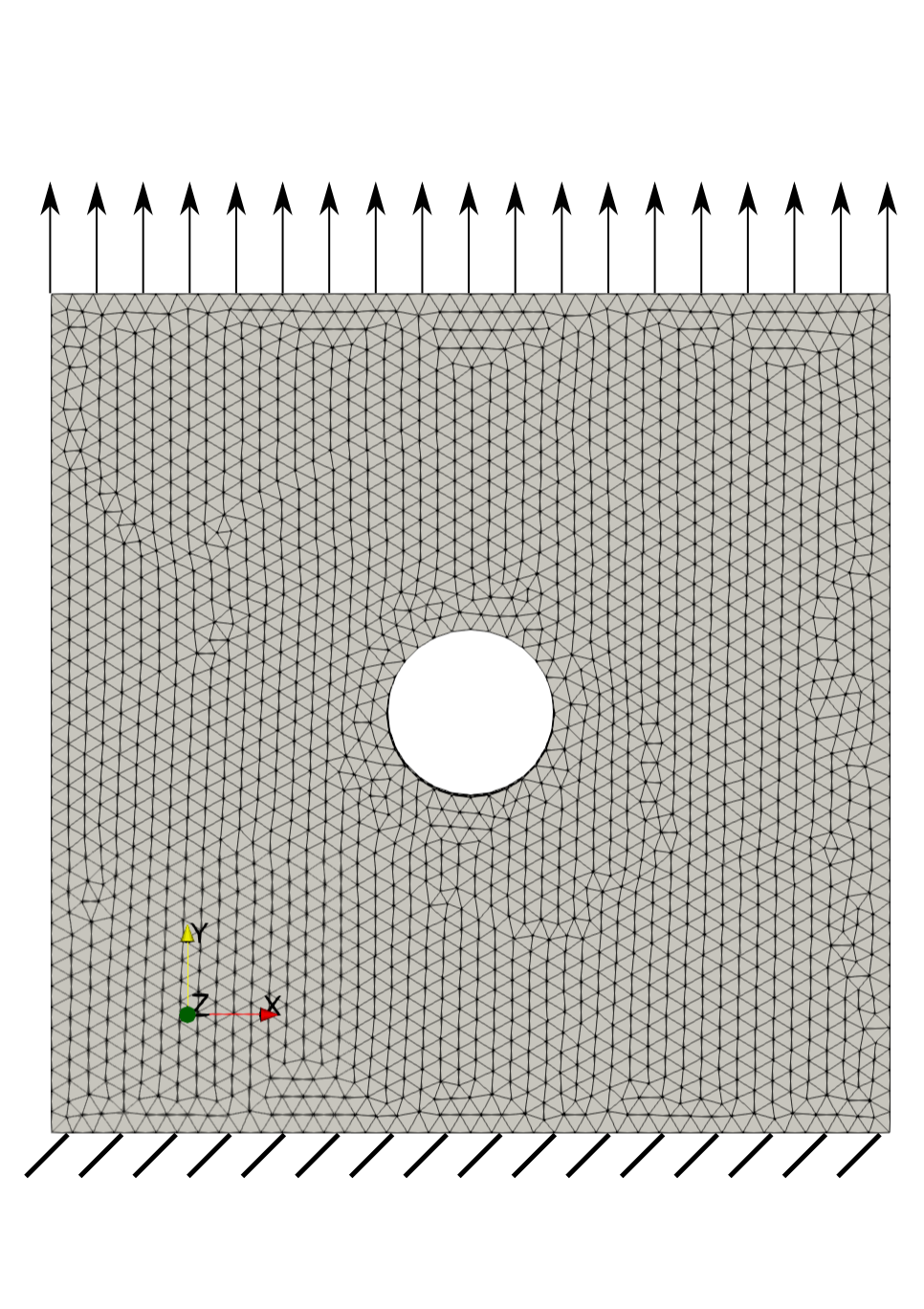
(a) The geometry, mesh, and boundary conditions $\boldsymbol{u}=0$ on the bottom and $h_{y}=t$ on the top. The DIC surface $\Gamma_{\text{DIC}}$ is the
visible plane.

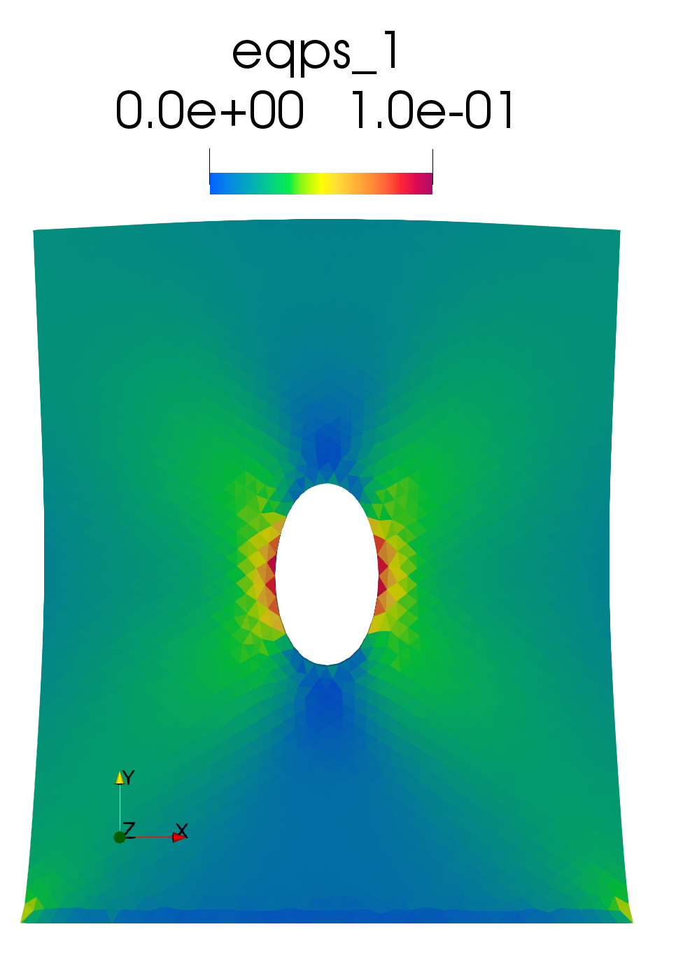
(b) The deformed geometry and equivalent plastic strain at the final load step with displacements exaggerated by a factor of 5.

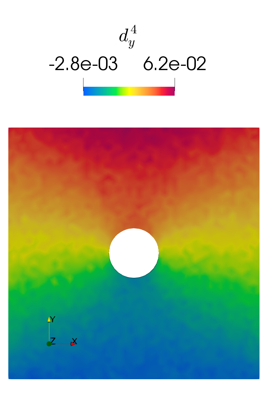
(c) The $y$-component of the noisy synthetic displacement data at the final load step.

Figure 1: Figures for the plate with a cylindrical hole example.

In this section, we provide several results that demonstrate the correctness of the objective function gradients obtained using forward and adjoint sensitivities. We consider a thin plate $[-1,1]\times[-1,1]\times[0,0.05]$ with a cylindrical hole of radius $r=0.2$ centered at the origin. The exact material model parameters are chosen to be

$$\boldsymbol{\beta}:=[E,\nu,Y,K,S,D]=[1000,0.25,2,100,0,0]$$ (33)

such that the governing constitutive response (3) reduces to one of isotropic linear hardening. The final two parameters $S$ and $D$ have been made “inactive” for the current results, meaning they are not considered as design variables. The domain is discretized using roughly thirteen thousand tetrahedral elements as shown in Figure 1(a). The traction boundary condition is defined by $h_{y}=t$, and the forward problem is run for $4$ load steps. Figure 1(b) illustrates an exaggerated version of the deformed geometry at the final load step.

As an initial step, we consider noiseless synthetic data and check the validity of the gradients obtained using forward (Algorithm 3) and adjoint (Algorithm 4) sensitivities via a comparison to the finite difference gradient (Algorithm 2). Concretely, this occurs by choosing a direction vector $\boldsymbol{D}$ and computing an error as the absolute value of the difference between the automatic differentiation gradient in the direction of this vector and the two-point centered finite difference gradient in the direction of this vector. Presently, we choose each component of this direction vector to be $D_{i}=0.1$. As an example, the error for the gradient obtained via adjoint sensitivities is computed as:

$$E_{\text{FD\_check}}=\left|\left(\left[\frac{d\mathcal{J}}{d\boldsymbol{\beta}}\right]_{\text{adjoint}}\cdot\boldsymbol{D}\right)-\left(\left[\frac{d\mathcal{J}}{d\boldsymbol{\beta}}\right]_{\text{FD}}\cdot\boldsymbol{D}\right)\right|$$ (34)

This error is computed using a variety of finite difference step sizes: $\varepsilon_{\text{FD}}=1,10^{-1},10^{-2},\dots,10^{-12}$ and the results are plotted in Figure 2. As is common with finite difference methods, we see the error in the finite difference approximation to the gradient decrease as the step size decreases until an inflection point at around $\varepsilon_{\text{FD}}=10^{-6}$, where round-off error begins to grow and the finite difference approximation loses accuracy. This is a known phenomena for computational finite difference methods, and its presence is a strong indication that the gradients computed by automatic differentiation are exact. Additionally, we remark that the errors for the gradient obtained with forward and adjoint sensitivities are numerically equivalent, indicating that the gradients computed with automatic differentiation are identical. This lends further credence to the notion that the correct gradients are computed when using the developed AD approaches.

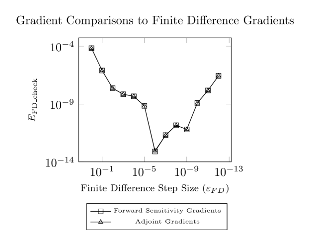
Figure 2: Finite difference gradient check for the plate with a cylindrical hole example.

As a second verification test, we set the parameters at an initial guess $\boldsymbol{\beta}_{0}=[1020,0.28,2.3,110.0,0,0]$ that is slightly different than the exact material parameters. We then use an L-BFGS-B algorithm to determine the material parameters that solve the optimization problem (21) using gradients obtained with forward finite differences, forward sensitivities, and adjoint sensitivities. Here, the lower and upper bounds have been chosen as $\boldsymbol{\beta}_{\text{lo}}=[900,0.2,0,90,0,0]$, and $\boldsymbol{\beta}_{\text{hi}}=[1200,0.4,10,150,0,0]$, respectively. For all three approaches, the L-BFGS-B algorithm terminates with zero percent relative error to at least eight significant digits for each design parameter. This provides further support of the correctness of the gradients computed with AD.

	$E$	$\nu$	$Y$	$K$	Time
Truth	1000	0.25	2	100	n/a
Initial	1020	0.28	2.3	110	n/a
$\epsilon^{*}_{\text{noise}}=$6.1\text{\times}{10}^{-5}$$
FEMU	1000.81 (0.081%)	0.2493 (0.277%)	1.9997 (0.016%)	99.9985 (0.002%)	103m23s
FS	1000.81 (0.081%)	0.2493 (0.277%)	1.9997 (0.016%)	99.9985 (0.002%)	21m25s
Adjoint	1000.81 (0.081%)	0.2493 (0.277%)	1.9997 (0.016%)	99.9985 (0.002%)	14m52s
$\epsilon_{\text{noise}}=$1\text{\times}{10}^{-3}$$
FEMU	1009.22 (0.922%)	0.2491 (0.376%)	1.9952 (0.234%)	100.006 (0.006%)	89m38s
FS	1009.22 (0.922%)	0.2491 (0.376%)	1.9952 (0.234%)	100.006 (0.006%)	18m43s
Adjoint	1009.22 (0.922%)	0.2491 (0.376%)	1.9952 (0.234%)	100.006 (0.006%)	13m12s

Table 1: Inverse problem solutions for the plate with a cylindrical hole problem with noisy synthetic data. Errors relative to the true solutions are reported next to the parameter values.

As a final demonstration, we consider two sets of noisy synthetic data with $\epsilon^{*}_{\text{noise}}=$6.1\text{\times}{10}^{-5}$$ and $\epsilon_{\text{noise}}=$1\text{\times}{10}^{-3}$$. The $y$-component of the noisier displacement dataset is shown in the right panel of Figure 1(c). The optimization problem (21) (with initial guess $\boldsymbol{\beta}_{0}$ and bounds $\boldsymbol{\beta}_{\text{lo}}$ and $\boldsymbol{\beta}_{\text{hi}}$) is then solved using finite difference (FEMU), forward sensitivity (FS), and adjoint-based gradients. Results obtained using the three methods are shown in Table 1. We observe that to the precision shown in the table each method obtains the same solution, but the newly developed AD-based approaches take roughly one fifth the time of the FEMU approach. As mentioned in the previous section, this cost savings comes from the replacement of full nonlinear solves in the FEMU approach with the auxiliary linear solves present in the other methods.

Lastly, we also investigated the sensitivity of the solution of the inverse problem to the initial guess and amount of noise in this example. Both noise-corrupted inverse problems were run using initial guesses generated from the first ten elements of the 2,3,5,7 Halton sequence transformed by the optimization bounds (a “well-spaced” set of samples). We found that for each noise level six of these initial guesses resulted in the same solutions given in Table 1. The other four initial guesses had a $Y>=6$, and consequently produced forward solutions with comparatively smaller amounts of plastic deformation in the material. In some cases there was no plastic deformation until the last one or two load steps, and while the magnitude of the equivalent plastic strain was non-zero it was still diminutive and only present in a small percentage of elements. The reduction in the value of the objective function for these problems was extremely slow compared to that witnessed for the other initial guesses. In light of these observations, we recommend choosing a value of $Y$ that results in an appreciable amount of plastic strain in the material when the goal is to calibrate an elastoplastic constitutive model. These results also suggest that the minimum is unique over the range of optimization bounds considered in this example. In practice these bounds should be determined by a combination of expert knowledge (e.g. appropriate ranges for steel variants) and trial-and-error based on optimizer performance, as it is conceivable that for some problem configurations (i.e. specimen design, loading, constitutive models, calibration parameters, data quality) the optimization problem will be non-convex.

4.2 Large Problem

In this section we demonstrate that the proposed AD-based adjoint inversion approach can be used to perform material model calibration for large-scale simulations that would be otherwise intractable using finite difference-based FEMU. In particular, we consider a rectangular prism specimen $[0,0.25]\times[-1.625,1.625]\times[0,0.124]$ with three notches of varying sizes near the middle of the specimen (described in [77]) that introduce heterogeneity into the response. Figure 3(b) shows a picture of the undeformed sample. The geometry is discretized with over one million tetrahedral elements.

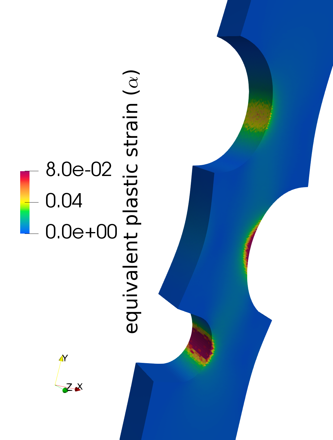
(a) The deformed geometry and the equivalent plastic strain at the final (tenth) load step.

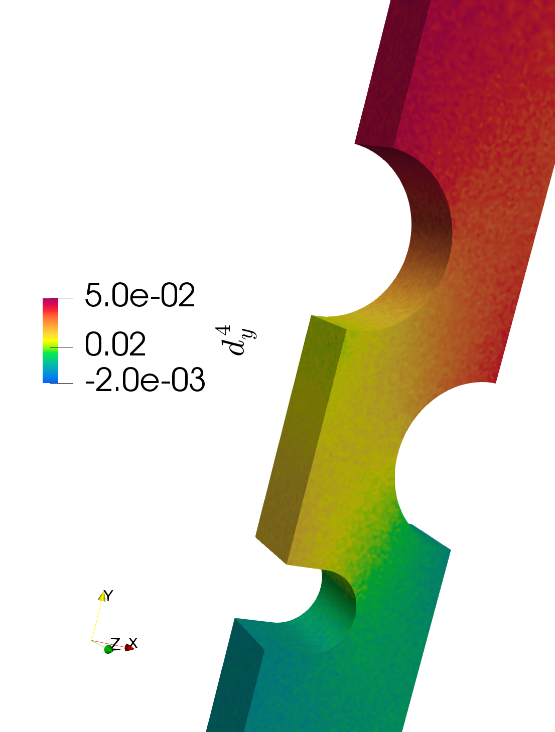
(b) The $y$-component of the noisy synthetic data computed with $\epsilon_{\text{noise}}=0.001$ at the fourth load step.

(c) The $y$-component of the noisy synthetic data computed with $\epsilon_{\text{noise}}=0.002$ at the fourth load step.

Figure 3: Figures for the large example problem.

The forward problem is defined by the traction boundary condition $h_{y}=2t$ and was run for a total of ten load steps, with exact material parameters defined as $\boldsymbol{\beta}=[E,\nu,Y,S,D]=[1000,0.32,6,120,100]$. Here the linear hardening parameter $K$ has been set to zero and non-zero values for $S$ and $D$ have been specified to induce Voce hardening in the specimen. The equivalent plastic strain $\alpha$ on the deformed geometry is shown in Figure 3(a). We consider three sets of noisy synthetic data, created using $\epsilon^{*}_{\text{noise}}=$1\text{\times}{10}^{-4}$$, $\epsilon_{\text{noise}}=$1\text{\times}{10}^{-3}$$, and $\epsilon_{\text{noise}}=$2\text{\times}{10}^{-3}$$. For the two noisier sets, the $y$-component of the noisy displacement data at the fourth load step is shown in Figures 3(b) and 3(c). In subsequent load steps, it is more difficult to see the noise in the data.

The optimization problem (21) was solved using adjoint-based gradients for all sets of noisy synthetic data. The initial parameters for the inverse problem were chosen to be $\boldsymbol{\beta}_{0}=[1200,0.36,3.5,105,80]$, with lower and upper bounds specified as $\boldsymbol{\beta}_{\text{lo}}=[800,0.25,3,100,60]$ and $\boldsymbol{\beta}_{\text{hi}}=[1600,0.4,10,150,200]$, respectively. For these model calibration runs, the parameter $K$ was been made “inactive”. The inverse problems were solved in parallel using 64 MPI ranks, and took roughly 9 or 12 hours to run using the adjoint and forward sensitivities approaches, respectively.

	$E$	$\nu$	$Y$	$S$	$D$
Truth	1000	0.32	6	120	100
Initial	1200	0.36	3.5	105	80
$\epsilon^{*}_{\text{noise}}$ = $1\text{\times}{10}^{-4}$	999.9 (0.006%)	0.32 (0.09%)	5.996 (0.06%)	119.95 (0.042%)	100.18 (0.18%)
$\epsilon_{\text{noise}}$ = $1\text{\times}{10}^{-3}$	998.8 (0.13%)	0.33 (1.74%)	6.17 (2.75%)	119.94 (0.046%)	100.5 (0.50%)
$\epsilon_{\text{noise}}$ = $2\text{\times}{10}^{-3}$	1011.5 (1.15%)	0.31 (4.13%)	4.70 (21.7%)	121.18 (0.98%)	92.94 (7.06%)

Table 2: Inverse problem solutions for the large-scale example problem with noisy synthetic data. Errors relative to the true solutions are reported next to the parameter values.

The results of the inverse problems are given in Table 2. As expected, the accuracy of the solution decreases as the amount of random noise in the data is increased. However, we note that each parameter is affected differently. For example, the saturation rate $D$ appears to be more sensitive to the presence of noise than the saturation modulus $S$, which suggests that the overall sensitivity of these parameters given the “experimental” setup is not equal. Although we do not explore this line of investigation in this work, global sensitivity analyses could be useful in designing experiments that exhibit high (and possibly more equal) sensitivity to all of the parameters of interest.

Finally, we remark that our demonstration of inversion with a mesh consisting of over one million elements is larger than we have encountered in the full-field model calibration literature. This is most likely due to the costs incurred by finite difference approximations. Ten load steps, however, is a rather small amount of DIC data when compared to the literature. Given that the focus of this paper is a demonstration of feasibility, we leave further exploration of the HPC aspects to future work. This work could include tackling the challenges of using many load steps, along with other technical hurdles that we elaborate on in Section 5.

4.3 Hypoelastic Model with Anisotropic Yield

As a final example, we showcase how our AD-based framework makes the implementation of finite deformation elastoplastic FE model with the Hill anisotropic yield function and elastic behavior described by a hypoelastic model below yield nearly trivial, as all that is required is an appropriate specification of the global and local residuals. In this section we present these residuals and then utilize them in a FE model that emulates a mechanical characterization experiment for a bi-axial test specimen with non-proportional loading where the goal is to estimate the in-plane anisotropy coefficients given synthetic DIC measurements with noise levels commensurate with those found in real experimental data.

Our use of a hypoelastic model in this example is motivated by several factors. First, some well-known disadvantages of these models (as compared to hyperelastic models) are their non-conservative nature and required use of an incrementally-objective integration algorithm for the rate of stress. The energy error introduced by the former, however, is negligible when the elastic strains are small compared to the plastic strains [13], as is the case in many problems of practical importance (e.g. sheet metal forming). Second, the proper treatment of anisotropic plasticity (i.e. anisotropic yield and/or distortional hardening) is arguably more challenging when described by a hyperelastic model [103], whereas with hypoelastic formulations it is straightforward to develop finite deformation versions of such models from small strain descriptions. Lastly, the presentation of a hypoelastic model in this section serves to highlight both the applicability of our AD-based approach to both classes of model formulations (encompassing all of those used in practice) while demonstrating relative ease with which it can be applied to a specific model of interest.

The global residual $\boldsymbol{R}$ is similar to (9) but due to our use of a hypoelastic model we can no longer derive expressions for the Kirchhoff stress and pressure from a strain-energy density function. We instead introduce a split in the hydrostatic and deviatoric parts of the Cauchy stress

$$\boldsymbol{\sigma}=\text{dev}(\boldsymbol{\sigma})+\frac{\text{tr}(\boldsymbol{\sigma})}{3}\boldsymbol{I}=\text{dev}(\boldsymbol{\sigma})-p\boldsymbol{I}$$ (35)

to allow for the equal-order interpolation of the displacement and pressure fields via stabilization as was done in the hyperelastic-plastic formulation presented previously.

We change the local state variables vector to include the unrotated Cauchy stress $\boldsymbol{T}$ and equivalent plastic strain $\alpha$ such that $\boldsymbol{\xi}:=\{\boldsymbol{T},\alpha\}$. Due to the symmetry of $\boldsymbol{T}$, $\boldsymbol{\xi}$ has seven independent components. The Cauchy stress $\boldsymbol{\sigma}$ and $\boldsymbol{T}$ are related through the polar decomposition of the deformation gradient

$$\begin{aligned} \boldsymbol{F}&=\boldsymbol{R}\boldsymbol{U},\\ \boldsymbol{T}&=\boldsymbol{R}^{T}\boldsymbol{\sigma}\boldsymbol{R}.\end{aligned}$$ (36)

The stabilized global residual $\boldsymbol{R}$ is

$$\begin{split}&\int_{\mathcal{B}}(J\ (\text{dev}\left[\boldsymbol{R}\boldsymbol{T}\boldsymbol{R}^{T}\right]-p\boldsymbol{I})\ \boldsymbol{F}^{-T}):\nabla\boldsymbol{w}\,\text{d}V-\int_{\mathcal{B}}\left(p+\frac{\text{tr}\left[\boldsymbol{R}\boldsymbol{T}\boldsymbol{R}^{T}\right]}{3}\right)q\,\text{d}V-\\ &\sum_{e=1}^{n_{el}}\int_{\mathcal{B}_{e}}\tau_{e}(J\boldsymbol{F}^{-1}\boldsymbol{F}^{-T}):(\nabla p\otimes\nabla q)\,\text{d}V-\int_{\Gamma_{h}}\boldsymbol{h}\cdot\boldsymbol{w}\,\,\text{d}A=0,\end{split}$$ (37)

where all of the quantities are discretized at the current time step (superscript $n$ omitted for brevity), and the finite element spaces are the same as those stated previously in (8).

Following [101] and the references therein, we utilize the Green-McInnis stress rate for objective integration of the rate of the Cauchy stress through a corotational formulation, which involves the use of the polar decomposition of the deformation gradient at the current time step. The relevant kinematics expressed in discrete form using a backward Euler discretization are

$$\begin{aligned} \boldsymbol{F}^{n}&=\boldsymbol{R}^{n}\boldsymbol{U}^{n},\\ \boldsymbol{L}^{n}&=\left(\boldsymbol{F}^{n}-\boldsymbol{F}^{n-1}\right)\left(\boldsymbol{F}^{n}\right)^{-1},\\ \boldsymbol{D}^{n}&=\frac{1}{2}\left(\boldsymbol{L}^{n}+\left(\boldsymbol{L}^{n}\right)^{T}\right),\\ \boldsymbol{d}^{n}&=\left(\boldsymbol{R}^{n}\right)^{T}\boldsymbol{D}^{n}\boldsymbol{R}^{n},\end{aligned}$$ (38)

where $\boldsymbol{L}$ is the velocity gradient, $\boldsymbol{D}$ is the rate of deformation tensor, and $\boldsymbol{d}$ is the unrotated rate of deformation tensor.

Hypoelastic constitutive models assume an additive decomposition of $\boldsymbol{d}$ into elastic $\boldsymbol{d}^{e}$ and plastic $\boldsymbol{d}^{p}$ components. The backwards Euler temporal discretization of the constitutive equation for an isotropic hypoelastic material expressed in rate form in the unrotated configuration is

$$\begin{aligned} \boldsymbol{d}^{n}&=\left(\boldsymbol{d}^{e}\right)^{n}+\left(\boldsymbol{d}^{p}\right)^{n},\\ \boldsymbol{T}^{n}&=\boldsymbol{T}^{n-1}+\Delta t\left(\lambda\text{tr}\left[\left(\boldsymbol{d}^{e}\right)^{n}\right]\boldsymbol{I}+2\mu\left(\boldsymbol{d}^{e}\right)^{n}\right).\end{aligned}$$ (39)

The Hill [39] effective stress function $\phi$ contains six coefficients $F,G,H,L,M,$ and $N$

$$\phi(T_{ij})=\left(F\left(T_{22}-T_{33}\right)^{2}+G\left(T_{33}-T_{11}\right)^{2}+H\left(T_{11}-T_{22}\right)^{2}+2L\left(T_{23}\right)^{2}+2M\left(T_{13}\right)^{2}+2N\left(T_{12}\right)^{2}\right)^{\frac{1}{2}},$$ (40)

that are defined in terms of a reference yield stress $Y$ and 6 independent axial $\sigma^{y}_{ii}$ and shear $\tau^{y}_{ij}$ yield stresses such that

$$\begin{aligned} F&=\frac{Y^{2}}{2}\left(\left(\sigma^{y}_{22}\right)^{-2}+\left(\sigma^{y}_{33}\right)^{-2}-\left(\sigma^{y}_{11}\right)^{-2}\right),\quad L=\frac{Y^{2}}{2}\left(\tau^{y}_{23}\right)^{-2},\\ G&=\frac{Y^{2}}{2}\left(\left(\sigma^{y}_{33}\right)^{-2}+\left(\sigma^{y}_{11}\right)^{-2}-\left(\sigma^{y}_{22}\right)^{-2}\right),\quad M=\frac{Y^{2}}{2}\left(\tau^{y}_{13}\right)^{-2},\\ H&=\frac{Y^{2}}{2}\left(\left(\sigma^{y}_{11}\right)^{-2}+\left(\sigma^{y}_{22}\right)^{-2}-\left(\sigma^{y}_{33}\right)^{-2}\right),\quad N=\frac{Y^{2}}{2}\left(\tau^{y}_{12}\right)^{-2}.\end{aligned}$$ (41)

For calibration purposes we express the constitutive model parameters in terms of the six independent quantities $R_{ij}$ defined to be

$$R_{ii}=\frac{\sigma_{ii}^{y}}{Y}\quad\text{for}\ i=1,2,3,\qquad R_{ij}=\sqrt{3}\frac{\tau^{y}_{ij}}{Y}\quad\text{for}\ i,j=1,2,3,\ \text{and}\ i<j.$$ (42)

The Hill yield function (40) is equivalent to the $J_{2}$ yield function when $R_{ij}=1\ \forall i,j$. The discretized flow rule and hardening law may be combined to obtain

$$\left(\boldsymbol{d}^{p}\right)^{n}=\Delta\gamma^{n}\frac{\partial\phi^{n}}{\partial\boldsymbol{T}^{n}}=\frac{1}{\Delta t}\left(\alpha^{n}-\alpha^{n-1}\right)\frac{\partial\phi^{n}}{\partial\boldsymbol{T}^{n}}.$$ (43)

We note that for this model $\text{tr}\left[\left(\boldsymbol{d}^{p}\right)^{n}\right]=0$ [23].

In this final example we assume isotropic linear hardening. The value of the yield function for the trial elastic step $f^{n}_{\text{trial}}=\phi^{n}_{\text{trial}}-Y-K\alpha_{\text{trial}}$ is obtained by assuming the rate of deformation is completely elastic (i.e. $\boldsymbol{d}^{n}=\left(\boldsymbol{d}^{e}\right)^{n}$) in (39) and $\alpha_{\text{trial}}=\alpha^{n-1}$. The discrete constitutive equation evolution equations $\boldsymbol{C}^{n}$ below yield (i.e. $f^{n}_{\text{trial}}<0$) are

$$\begin{cases}\begin{aligned} &\boldsymbol{T}^{n}-\boldsymbol{T}^{n-1}-\Delta t\left(\lambda\text{tr}\left[\boldsymbol{d}^{n}\right]\boldsymbol{I}+2\mu\boldsymbol{d}^{n}\right)=\boldsymbol{0},\\ &\alpha^{n}-\alpha^{n-1}=0.\end{aligned}\end{cases}$$ (44)

When plastic flow occurs they are

$$\begin{cases}\begin{aligned} &\boldsymbol{T}^{n}-\boldsymbol{T}^{n-1}-\Delta t\left(\lambda\text{tr}\left[\boldsymbol{d}^{n}\right]\boldsymbol{I}+2\mu\left(\boldsymbol{d}^{n}-\frac{1}{\Delta t}\left(\alpha^{n}-\alpha^{n-1}\right)\frac{\partial\phi^{n}}{\partial\boldsymbol{T}^{n}}\right)\right)=\boldsymbol{0},\\ &\phi^{n}(\boldsymbol{T}^{n})-Y-K\alpha^{n}=0.\end{aligned}\end{cases}$$ (45)

To summarize, the hypoelastic-plastic model with anisotropic yield utilizes global and local state residuals that are distinct from those described previously in this work, and the definition of the local state variables is different.

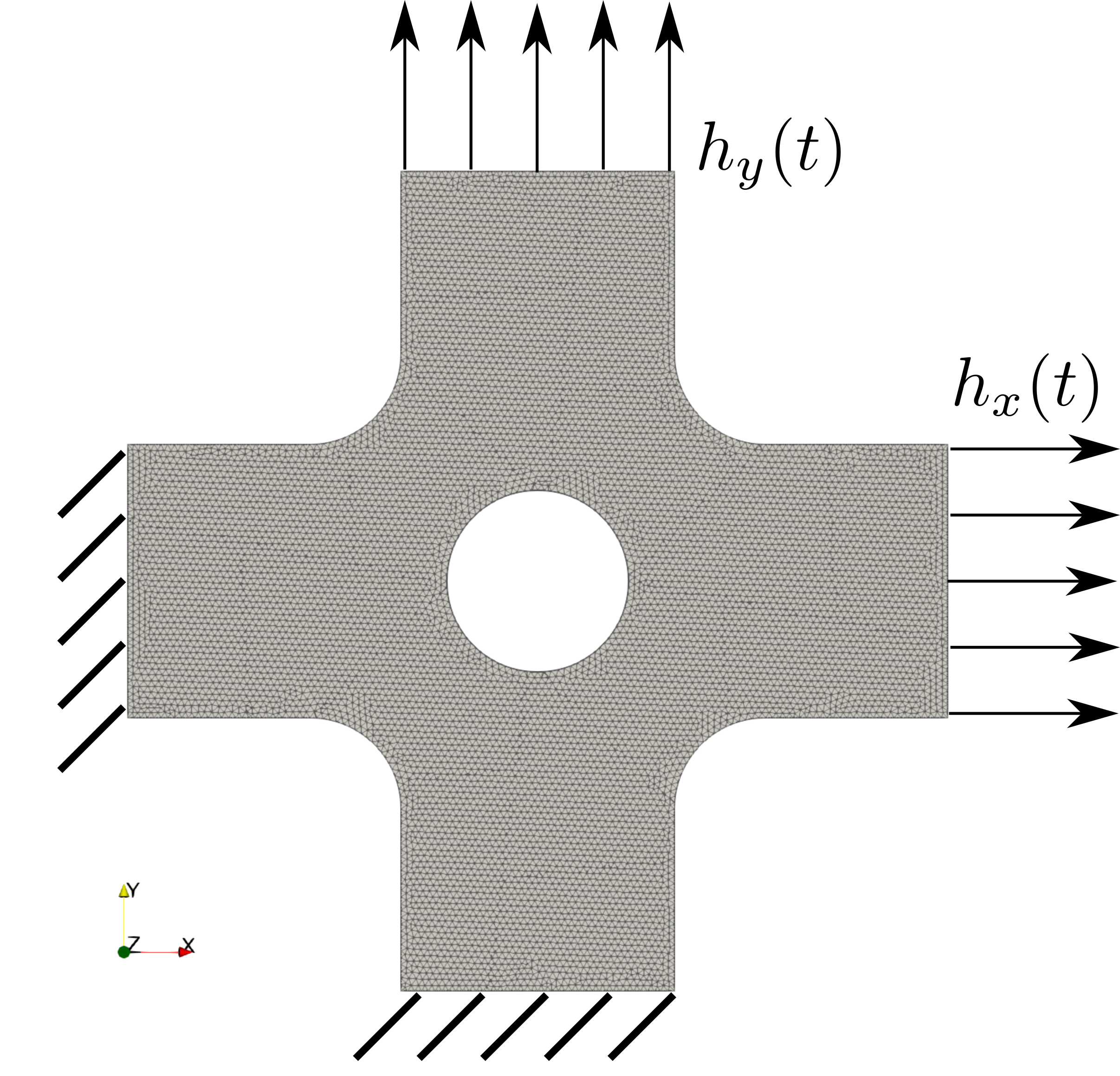
(a) The geometry, mesh, and boundary conditions $\boldsymbol{u}=\boldsymbol{0}$ on the bottom and left edges, $h_{y}(t)$ on the top edge, and $h_{x}(t)$ on the right edge. The DIC surface $\Gamma_{\text{DIC}}$ is the visible plane.

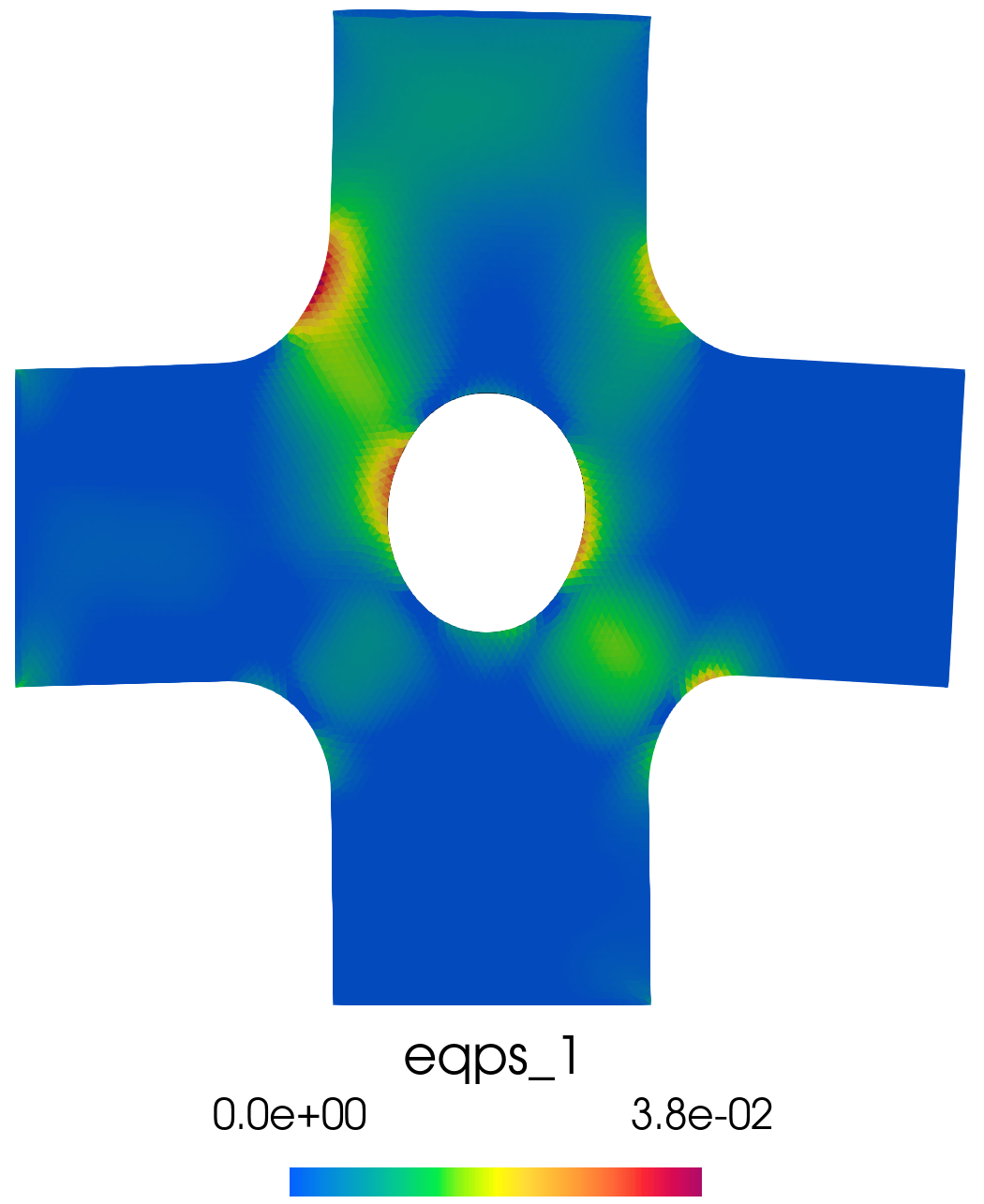
(b) The deformed geometry and equivalent plastic strain at the 6th load step with displacements exaggerated by a factor of 5.

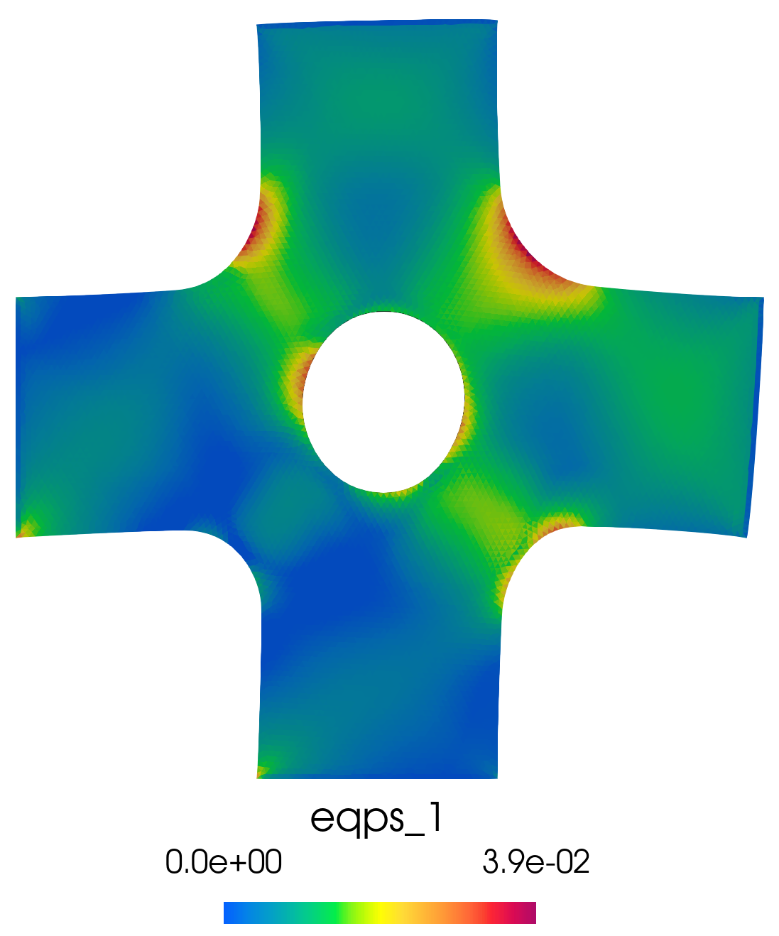
(c) The deformed geometry and equivalent plastic strain at the 12th load step with displacements exaggerated by a factor of 5.

Figure 4: Cruciform specimen geometry, FE model boundary conditions, and equivalent plastic strain under axial (middle) and bi-axial (right) loading.

We now present a FE model of a synthetic mechanical characterization experiment that consists of a cruciform test specimen subject to bi-axial loading with the aim of demonstrating the feasibility of our AD-based calibration methods for estimating parameters related to anisotropic yield. We utilize a cruciform specimen geometry that has been adapted from [20]. The dimensions of the bounding box that encloses it are $[-4.5,4.5]\times[-4.5,4.5]\times[0,0.12]$ and the radii of the circle in the center and fillets are all equal to 1. The test specimen was deformed non-proportionally over a series of 12 load steps according to the traction boundary conditions

$$\begin{aligned} &h_{x}=0,\ h_{y}=0.5t&&\text{for}\ t=1,\ldots,6,\\ &h_{x}=0.5(t-6),\ h_{y}=3\quad&&\text{for}\ t=7,\ldots,12.\end{aligned}$$ (46)

that are applied over the surfaces of the test specimen as depicted in Figure 4(a).

In this bi-axial example we set $R_{11}=1$ so that it is equal to the reference yield stress value $Y$. We also fix the out of plane shear parameters $R_{23}$ and $R_{13}$ to 1 because the out of plane shear stress in this problem is negligible compared to the in-plane stresses. The constitutive model parameters in this example are

$$\boldsymbol{\beta}=\left[E,\nu,Y,K,R_{11},R_{22},R_{33},R_{23},R_{13},R_{12}\right]=\left[1000,0.25,2,100,1,1.05,0.95,1,1,0.85\right].$$ (47)

Calibration results obtaining using finite difference FEMU and forward and adjoint sensitivities are reported in Table 3. All of the calibration problems were executed in parallel using 16 MPI ranks. The running times for the forward and adjoint sensitivities approaches were within minutes of each other for each noise case. They were (on average) 3.8 hours and 7.2 hours for the adjoint and forward sensitivities approaches, respectively. The optimization iteration count and number of objective function and gradient evaluations were the same for these methods, and this finding is consistent with our previous examples. The running times for the FEMU calibration problems, however, exhibited greater variability due to the finite difference approximation of the gradient although their parameter estimates were nearly identical to those obtained using the other two methods. The $\epsilon^{*}_{\text{noise}}=$2.7\text{\times}{10}^{-4}$$ and $\epsilon_{\text{noise}}=$1\text{\times}{10}^{-3}$$ FEMU problems took 36 hours and 29 hours, respectively.

	$E$	$\nu$	$Y$	$K$	$R_{22}$	$R_{33}$	$R_{12}$
Truth	1000	0.25	2	100	0.9	1.05	0.85
Initial	1020	0.28	2.3	110	0.95	0.95	0.95
$\epsilon^{*}_{\text{noise}}=$2.7\text{\times}{10}^{-4}$$
Parameter Value	1000.30	0.2504	1.9996	100.053	0.89997	1.0501	0.8501
Parameter Error (%)	0.03	0.153	0.019	0.053	0.001	0.008	0.018
$\epsilon_{\text{noise}}=$1\text{\times}{10}^{-3}$$
Parameter Value	998.92	0.2482	2.0007	99.879	0.89976	1.0494	0.8502
Parameter Error (%)	0.108	0.724	0.035	0.121	0.026	0.061	0.027

Table 3: Inverse problem solutions for the cruciform specimen problem with noisy synthetic data. Solutions obtained through each of the three inverse methods were the same to the precision shown in the table.

The accuracy of the recovered anisotropic coefficients is encouraging (all $R_{ij}$ are recovered to within 0.1 % error for both noise cases). These results and those obtained from our previous examples have given us confidence in our numerical formulation and its computational implementation and provided motivation to further develop our approach so that it may be applied to experimental DIC data.

5 Discussion

In this section we discuss a few aspects of our approach that would need to be extended for calibration with experimental DIC data to be successful. First, as discussed in section 3, the objective function in this work should be augmented with a force-matching term, and weighting functions are needed to properly account for the uncertainty in measurements of displacement and load. Second, the DIC algorithm filters the true displacement signal, and in many cases the data is projected onto the mesh/basis used in the FE model, which can corrupt the objective function in some instances [51]. Finally, in our formulation we synchronized load steps and DIC data frames and utilized idealized boundary conditions, and these restrictions should be relaxed.

Our formulation of the objective function is appropriate when the noise in each displacement measurement is i.i.d. Gaussian across all frames. The noise in our example problems conformed to this, but in real DIC measurements the noise exhibits spatial heterogeneity in some instances. In particular, the largest source of this variability occurs in local or subset-based DIC formulations, where the error in the projection of the DIC measurements onto the FE mesh ($\boldsymbol{d}$) is considerably higher near the boundaries of specimen. One way to address this issue is to decrease the influence of measurements in these regions through the use of a weighting function in the objective function that decays to zero around the boundaries. Alternatively, the DIC region-of-interest ($\Gamma_{\text{DIC}}$) could be suitably redefined. Second, when a force-matching term is present, care must be taken to properly balance it with the displacement-matching piece, which can be challenging when the noise in either term is not normally-distributed.

There are also a few technical details related to the nature of the real DIC measurements that we avoided in our presentation. First, in local (subset-based) and global (FE-based) DIC formulations, it is often the case that the basis that represents the DIC displacements is not the same as that used in the FE model, which necessitates interpolation between the DIC point cloud (local) or FE basis (global) to the FE basis for the model. In local DIC the point cloud of measurements is typically very dense, such that interpolation error is unlikely to be a problem unless the FE mesh is extremely fine. Integrated DIC often uses a global formulation where the same mesh is used for both the DIC and model calibration components of the formulation, but projection operators between meshes can be introduced into the inverse formulation if distinct bases are desired. The DIC algorithm can be viewed as low-pass filter on the true deformation field in both a spatial and temporal sense. Consequently, measurements with high spatial gradients and/or rapid temporal variations may be biased, and these limitations should be taken into account when designing aspects of the mechanical test (e.g. motion of grips, image acquisition rate). Lastly, the DIC algorithm itself has several user-defined parameters such as subset or element size and basis function order that can affect the amount of random and bias errors present in the DIC measurements.

In this work we treated the BCs on the specimen as known and imposed them directly in the equilibrium equation, but in real experiments choosing what BCs to utilize in the forward model can be difficult. They can be idealized, but this choice can lead to errors when the experimental configuration deviates from the assumed BCs (which is often the case even in well-controlled experiments). The DIC data provides a source of Dirichlet boundary conditions on the DIC surface, and in the case of thin planar specimens, it may be reasonable to extend the in-plane displacements through the thickness in a 3D FE model. Alternatively, for a thin sample a plane stress model may be appropriate, but its use would require a modified version of the forward formulation that incorporates the plane stress condition as a constraint. For thicker specimens, another option is to set up two back-to-back stereo DIC systems to measure displacements on both sides of a planar sample so that displacement measurements can be interpolated through the thickness of the specimen, thus providing all components of the displacement BCs over the Dirichlet surface [44]. Finally, as mentioned in the previous paragraph, while DIC measurements are typically high-quality, they are not perfect and imposing them directly may introduce errors in the forward model.

The final modification is the relaxation of the requirement for the DIC measurements and FE model to share the same temporal discretization. In experiments images are typically acquired at a fixed rate. In many FE codes the nonlinear solver for the forward model is adaptive such that the time step can grow or shrink to improve the robustness of the code and promote computational efficiency. The temporal discretization of the FE model should be aligned with the DIC measurements in time, but it could be allowed to have additional steps. An alternative approach would be to perform temporal interpolation on the DIC data. The derivative of the objective function with respect to the displacement degrees of freedom would be zero for the steps that contain no DIC data.

6 Conclusion

In this paper we have described an approach for model calibration from DIC data based on a PDE-constrained optimization formulation with a finite element discretization in which the gradient is obtained through forward or adjoint sensitivity analyses. A challenge in the calibration of elastoplastic constitutive models is the treatment of the coupled nature of the equilibrium PDE, which is satisfied in a global sense, and local equations that govern the time evolution of the constitutive equation. While other studies in the topology optimization literature have considered similar coupled constraints, our reliance on AD to compute the derivatives needed for the forward problem and gradient calculation is novel and frees us from their laborious analytical derivation.

We have shown that both the forward and adjoint sensitivities-based algorithms for computing the gradient are accurate and dramatically reduce the cost of solving the inverse problem relative to using finite differences. Further, we have shown that our computational implementation is suitable for large-scale finite element models on HPC platforms. Promising directions for future work include increasing the computational efficiency of the forward sensitivities approach for use in large-scale problems with many load steps and applying an extended version of the inverse formulation to actual DIC data.

Finally, while computationally-efficient methods for computing gradients of quantities of interest are of course useful for PDE-constrained optimization problems like model calibration or topology optimization, they can also be used to produce more accurate surrogate models than those built using function evaluations alone. Similarly, the adjoint-based sensitivity analysis described in this paper could be modified for use in goal-oriented error estimation. Thus, the methods presented here may find application in areas other than the model calibration field focused on in this work.

Data Availability

The data that support the findings of this study are available from the corresponding author upon reasonable request.

Appendix A Optimization Details for the Numerical Examples

This appendix contains plots of the objective function histories and a table of function and gradient evaluations for each of the numerical examples presented in section 4. The problems in sections 4.1, 4.2, 4.3, are referred to as circle, large-scale, and cruciform, respectively. We only plot the objective function histories obtained from the adjoint approach, as those obtained with the forward sensitivities approach were identical and the finite difference FEMU results were extremely similar.

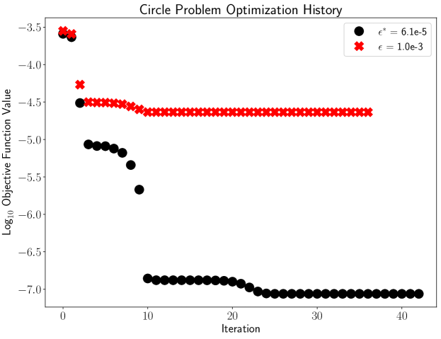
Figure 5: Circle example convergence.

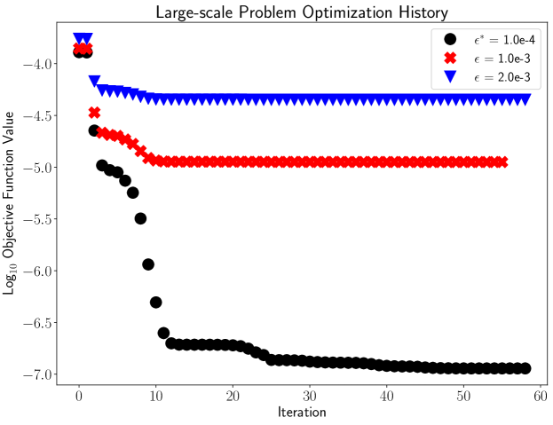
Figure 6: Large-scale example convergence.

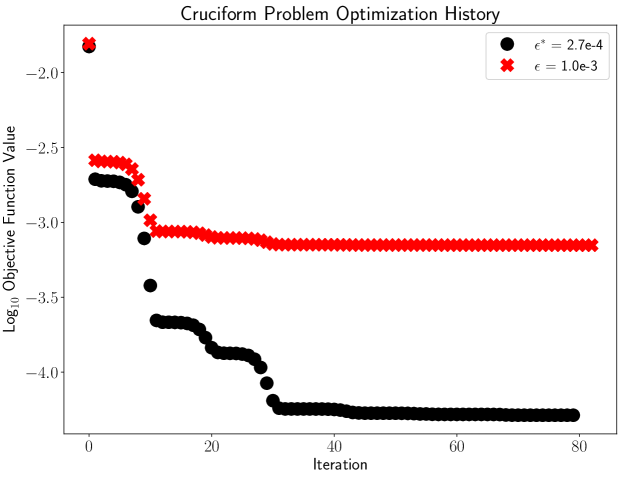
Figure 7: Cruciform example convergence.

	$\mathcal{J}$ Evaluations	$\frac{d\mathcal{J}}{d\boldsymbol{\beta}}$ Evaluations
Circle Problem
$\epsilon^{*}_{\text{noise}}=$6.1\text{\times}{10}^{-5}$$	44	43
$\epsilon_{\text{noise}}=$1.0\text{\times}{10}^{-3}$$	39	37
Large-scale Problem
$\epsilon^{*}_{\text{noise}}=$1.0\text{\times}{10}^{-4}$$	64	59
$\epsilon_{\text{noise}}=$1.0\text{\times}{10}^{-3}$$	68	56
$\epsilon_{\text{noise}}=$2.0\text{\times}{10}^{-3}$$	72	59
Cruciform Problem
$\epsilon^{*}_{\text{noise}}=$2.7\text{\times}{10}^{-4}$$	88 / 91	80 / 77
$\epsilon_{\text{noise}}=$1.0\text{\times}{10}^{-3}$$	89 / 69	83 / 60

Table 4: Number of objective function $\mathcal{J}$ and gradient $\frac{d\mathcal{J}}{d\boldsymbol{\beta}}$ evaluations for each of the numerical examples. The evaluations reported for the forward sensitivities and adjoint methods (FS-ADJ) were identical but distinct from the FEMU results in the cruciform example, so they are reported separately (i.e. FS-ADJ / FEMU). A comparison to FEMU was not performed for the large-scale example.

References

- [1] Swagato Acharjee and Nicholas Zabaras. A proper orthogonal decomposition approach to microstructure model reduction in rodrigues space with applications to optimal control of microstructure-sensitive properties. Acta Materialia, 51(18):5627–5646, 2003.
- [2] Swagato Acharjee and Nicholas Zabaras. The continuum sensitivity method for the computational design of three-dimensional deformation processes. Computer Methods in Applied Mechanics and Engineering, 195(48-49):6822–6842, 2006.
- [3] Ryan Alberdi and Kapil Khandelwal. Topology optimization of pressure dependent elastoplastic energy absorbing structures with material damage constraints. Finite Elements in Analysis and Design, 133:42–61, 2017.
- [4] Ryan Alberdi and Kapil Khandelwal. Bi-material topology optimization for energy dissipation with inertia and material rate effects under finite deformations. Finite Elements in Analysis and Design, 164:18–41, 2019.
- [5] Ryan Alberdi and Kapil Khandelwal. Design of periodic elastoplastic energy dissipating microstructures. Structural and Multidisciplinary Optimization, 59(2):461–483, 2019.
- [6] Ryan Alberdi and Kapil Khandelwal. Optimized bi-material layouts for energy dissipating composites under finite deformations. International Journal of Solids and Structures, 193:152–171, 2020.
- [7] Ryan Alberdi, Guodong Zhang, Lei Li, and Kapil Khandelwal. A unified framework for nonlinear path-dependent sensitivity analysis in topology optimization. International Journal for Numerical Methods in Engineering, 115(1):1–56, 2018.
- [8] Oded Amir. Stress-constrained continuum topology optimization: a new approach based on elasto-plasticity. Structural and Multidisciplinary Optimization, 55(5):1797–1818, 2017.
- [9] Stéphane Avril, Marc Bonnet, Anne-Sophie Bretelle, Michel Grédiac, François Hild, Patrick Ienny, Félix Latourte, Didier Lemosse, Stéphane Pagano, Emmanuel Pagnacco, et al. Overview of identification methods of mechanical parameters based on full-field measurements. Experimental Mechanics, 48(4):381, 2008.
- [10] S Badrinarayanan and Nicholas Zabaras. A sensitivity analysis for the optimal design of metal-forming processes. Computer Methods in Applied Mechanics and Engineering, 129(4):319–348, 1996.
- [11] Brian K Bay. Methods and applications of digital volume correlation. The Journal of Strain Analysis for Engineering Design, 43(8):745–760, 2008.
- [12] Brian K Bay, Tait S Smith, David P Fyhrie, and Malik Saad. Digital volume correlation: three-dimensional strain mapping using x-ray tomography. Experimental mechanics, 39(3):217–226, 1999.
- [13] Ted Belytschko, Wing Kam Liu, Brian Moran, and Khalil Elkhodary. Nonlinear finite elements for continua and structures. John wiley & sons, 2013.
- [14] Morgan Bertin, François Hild, and Stéphane Roux. On the identifiability of hill-1948 plasticity model with a single biaxial test on very thin sheet. Strain, 53(5):e12233, 2017.
- [15] Morgan Bertin, François Hild, Stéphane Roux, Florent Mathieu, Hugo Leclerc, and Patrick Aimedieu. Integrated digital image correlation applied to elastoplastic identification in a biaxial experiment. The Journal of Strain Analysis for Engineering Design, 51(2):118–131, 2016.
- [16] Michael J Borden, Thomas JR Hughes, Chad M Landis, Amin Anvari, and Isaac J Lee. A phase-field formulation for fracture in ductile materials: Finite deformation balance law derivation, plastic degradation, and stress triaxiality effects. Computer Methods in Applied Mechanics and Engineering, 312:130–166, 2016.
- [17] Ante Buljac, Clément Jailin, Arturo Mendoza, Jan Neggers, Thibault Taillandier-Thomas, Amine Bouterf, Benjamin Smaniotto, François Hild, and Stéphane Roux. Digital volume correlation: review of progress and challenges. Experimental Mechanics, 58(5):661–708, 2018.
- [18] Ante Buljac, Victor-Manuel Trejo Navas, Modesar Shakoor, Amine Bouterf, Jan Neggers, Marc Bernacki, Pierre-Olivier Bouchard, Thilo F Morgeneyer, and François Hild. On the calibration of elastoplastic parameters at the microscale via x-ray microtomography and digital volume correlation for the simulation of ductile damage. European Journal of Mechanics-A/Solids, 72:287–297, 2018.
- [19] Qiushi Chen, Jakob T Ostien, and Glen Hansen. Automatic differentiation for numerically exact computation of tangent operators in small-and large-deformation computational inelasticity. In TMS 2014: 143rd Annual Meeting & Exhibition, pages 289–296. Springer, 2014.
- [20] Sam Coppieters, Tomoyuki Hakoyama, Dimitri Debruyne, Susumu Takahashi, and Toshihiko Kuwabara. Inverse yield locus identification of sheet metal using a complex cruciform in biaxial tension and digital image correlation. In multidisciplinary digital publishing institute proceedings, volume 2, page 382, 2018.
- [21] Brendan P Croom, Huiqing Jin, Bernice Mills, and Xiaodong Li. Effect of fragile speckle patterns on accuracy of digital volume correlation. Experimental Mechanics, 59(7):991–1005, 2019.
- [22] ERIC C Cyr, JN Shadid, and T Wildey. Towards efficient backward-in-time adjoint computations using data compression techniques. Computer Methods in Applied Mechanics and Engineering, 288:24–44, 2015.
- [23] Eduardo A de Souza Neto, Djordje Peric, and David RJ Owen. Computational methods for plasticity: theory and applications. John Wiley & Sons, 2011.
- [24] Cetin B Dilgen, Sumer B Dilgen, David R Fuhrman, Ole Sigmund, and Boyan S Lazarov. Topology optimization of turbulent flows. Computer Methods in Applied Mechanics and Engineering, 331:363–393, 2018.
- [25] Sumer B Dilgen, Cetin B Dilgen, David R Fuhrman, Ole Sigmund, and Boyan S Lazarov. Density based topology optimization of turbulent flow heat transfer systems. Structural and Multidisciplinary Optimization, 57(5):1905–1918, 2018.
- [26] Felipe Fernandez and Daniel A Tortorelli. Semi-analytical sensitivity analysis for nonlinear transient problems. Structural and Multidisciplinary Optimization, 58(6):2387–2410, 2018.
- [27] Shankar Ganapathysubramanian and Nicholas Zabaras. A continuum sensitivity method for finite thermo-inelastic deformations with applications to the design of hot forming processes. International Journal for Numerical Methods in Engineering, 55(12):1391–1437, 2002.
- [28] Shankar Ganapathysubramanian and Nicholas Zabaras. Computational design of deformation processes for materials with ductile damage. Computer Methods in Applied Mechanics and Engineering, 192(1-2):147–183, 2003.
- [29] Shankar Ganapathysubramanian and Nicholas Zabaras. Deformation process design for control of microstructure in the presence of dynamic recrystallization and grain growth mechanisms. International journal of solids and structures, 41(7):2011–2037, 2004.
- [30] Shankar Ganapathysubramanian and Nicholas Zabaras. Design across length scales: a reduced-order model of polycrystal plasticity for the control of microstructure-sensitive material properties. Computer Methods in Applied Mechanics and Engineering, 193(45-47):5017–5034, 2004.
- [31] Pedro Gomes and Rafael Palacios. Aerodynamic-driven topology optimization of compliant airfoils. Structural and Multidisciplinary Optimization, 2020.
- [32] Brian N Granzow, Assad A Oberai, and Mark S Shephard. Adjoint-based error estimation and mesh adaptation for stabilized finite deformation elasticity. Computer Methods in Applied Mechanics and Engineering, 337:263–280, 2018.
- [33] Michel Grediac, Fabrice Pierron, Stéphane Avril, and Evelyne Toussaint. The virtual fields method for extracting constitutive parameters from full-field measurements: a review. Strain, 42(4):233–253, 2006.
- [34] Andreas Griewank and Andrea Walther. Evaluating derivatives: principles and techniques of algorithmic differentiation. SIAM, 2008.
- [35] Jason Hicken and Juan Alonso. Comparison of reduced-and full-space algorithms for pde-constrained optimization. In 51st AIAA Aerospace Sciences Meeting including the New Horizons Forum and Aerospace Exposition, page 1043, 2013.
- [36] François Hild, Amine Bouterf, Ludovic Chamoin, Hugo Leclerc, Florent Mathieu, Jan Neggers, Florent Pled, Zvonimir Tomičević, and Stéphane Roux. Toward 4d mechanical correlation. Advanced Modeling and Simulation in Engineering Sciences, 3(1):17, 2016.
- [37] François Hild and Stéphane Roux. Digital image correlation: from displacement measurement to identification of elastic properties–a review. Strain, 42(2):69–80, 2006.
- [38] François Hild and Stéphane Roux. Comparison of local and global approaches to digital image correlation. Experimental Mechanics, 52(9):1503–1519, 2012.
- [39] Rodney Hill. A theory of the yielding and plastic flow of anisotropic metals. Proceedings of the Royal Society of London. Series A. Mathematical and Physical Sciences, 193(1033):281–297, 1948.
- [40] Niklas Ivarsson, Mathias Wallin, and Daniel Tortorelli. Topology optimization of finite strain viscoplastic systems under transient loads. International Journal for Numerical Methods in Engineering, 114(13):1351–1367, 2018.
- [41] Niklas Ivarsson, Mathias Wallin, and Daniel A Tortorelli. Topology optimization for designing periodic microstructures based on finite strain viscoplasticity. Structural and Multidisciplinary Optimization, 61:2501–2521, 2020.
- [42] Elizabeth MC Jones, Kyle N Karlson, and Phillip L Reu. Investigation of assumptions and approximations in the virtual fields method for a viscoplastic material model. Strain, 55(4):e12309, 2019.
- [43] E.M.C. Jones, J.D. Carroll, K.N. Karlson, S.L.B. Kramer, R.B. Lehoucq, P.L. Reu, and D.Z. Turner. Parameter covariance and non-uniqueness in material model calibration using the virtual fields method. Comp. Mater. Sci., 152:268–290, 2018. doi:10.1016/j.commatsci.2018.05.037.
- [44] EMC Jones, Edmundo Corona, Amanda R Jones, William M Scherzinger, and Sharlotte Lorraine Bolyard Kramer. Anisotropic plasticity model forms for extruded al 7079: Part ii, validation. International Journal of Solids and Structures, 213:148–166, 2021.
- [45] Ottmar Klaas, Antoinette Maniatty, and Mark S Shephard. A stabilized mixed finite element method for finite elasticity.: Formulation for linear displacement and pressure interpolation. Computer Methods in Applied Mechanics and Engineering, 180(1-2):65–79, 1999.
- [46] Jože Korelc. Automation of primal and sensitivity analysis of transient coupled problems. Computational mechanics, 44(5):631–649, 2009.
- [47] Jože Korelc and Stanisław Stupkiewicz. Closed-form matrix exponential and its application in finite-strain plasticity. International Journal for Numerical Methods in Engineering, 98(13):960–987, 2014.
- [48] Joze Korelc and Peter Wriggers. Automation ofFinite Element Methods. Springer, 2016.
- [49] Sharlotte LB Kramer and William M Scherzinger. Implementation and evaluation of the virtual fields method: determining constitutive model parameters from full-field deformation data. Technical report, Sandia National Lab.(SNL-NM), Albuquerque, NM (United States), 2014.
- [50] Deepak V Kulkarni, Daniel A Tortorelli, and Mathias Wallin. A newton–schur alternative to the consistent tangent approach in computational plasticity. Computer methods in applied mechanics and engineering, 196(7):1169–1177, 2007.
- [51] Pascal Lava, Elizabeth MC Jones, Lukas Wittevrongel, and Fabrice Pierron. Validation of finite-element models using full-field experimental data: Levelling finite-element analysis data through a digital image correlation engine. Strain, 56(4):e12350, 2020.
- [52] David Lecompte, Steven Cooreman, Sam Coppieters, John Vantomme, Hugo Sol, and Dimitri Debruyne. Parameter identification for anisotropic plasticity model using digital image correlation: Comparison between uni-axial and bi-axial tensile testing. European Journal of Computational Mechanics/Revue Européenne de Mécanique Numérique, 18(3-4):393–418, 2009.
- [53] Lei Li and Kapil Khandelwal. Design of fracture resistant energy absorbing structures using elastoplastic topology optimization. Structural and Multidisciplinary Optimization, 56(6):1447–1475, 2017.
- [54] Lei Li, Guodong Zhang, and Kapil Khandelwal. Design of energy dissipating elastoplastic structures under cyclic loads using topology optimization. Structural and Multidisciplinary Optimization, 56(2):391–412, 2017.
- [55] Lei Li, Guodong Zhang, and Kapil Khandelwal. Topology optimization of energy absorbing structures with maximum damage constraint. International Journal for Numerical Methods in Engineering, 112(7):737–775, 2017.
- [56] Lei Li, Guodong Zhang, and Kapil Khandelwal. Failure resistant topology optimization of structures using nonlocal elastoplastic-damage model. Structural and Multidisciplinary Optimization, pages 1–30, 2018.
- [57] Zhen Li, Max O Bloomfield, and Assad A Oberai. Simulation of finite-strain inelastic phenomena governed by creep and plasticity. Computational Mechanics, 62(3):323–345, 2018.
- [58] Jikai Liu, Andrew T Gaynor, Shikui Chen, Zhan Kang, Krishnan Suresh, Akihiro Takezawa, Lei Li, Junji Kato, Jinyuan Tang, Charlie CL Wang, et al. Current and future trends in topology optimization for additive manufacturing. Structural and Multidisciplinary Optimization, 57(6):2457–2483, 2018.
- [59] Quan Long, Mohammad Motamed, and Raúl Tempone. Fast bayesian optimal experimental design for seismic source inversion. Computer Methods in Applied Mechanics and Engineering, 291:123–145, 2015.
- [60] Rolf Mahnken. Aspects on the finite-element implementation of the gurson model including parameter identification. International Journal of Plasticity, 15(11):1111–1137, 1999.
- [61] Rolf Mahnken. A comprehensive study of a multiplicative elastoplasticity model coupled to damage including parameter identification. Computers & Structures, 74(2):179–200, 2000.
- [62] Rolf Mahnken. Theoretical, numerical and identification aspects of a new model class for ductile damage. International Journal of Plasticity, 18(7):801–831, 2002.
- [63] Rolf Mahnken and Erwin Stein. Parameter identification for finite deformation elasto-plasticity in principal directions. Computer Methods in Applied Mechanics and Engineering, 147(1-2):17–39, 1997.
- [64] Antoinette M Maniatty, Yong Liu, Ottmar Klaas, and Mark S Shephard. Higher order stabilized finite element method for hyperelastic finite deformation. Computer methods in applied mechanics and engineering, 191(13-14):1491–1503, 2002.
- [65] A Marek, FM Davis, J-H Kim, and F Pierron. Experimental validation of the sensitivity-based virtual fields for identification of anisotropic plasticity models. Experimental Mechanics, pages 1–26, 2020.
- [66] JMP Martins, A Andrade-Campos, and S Thuillier. Calibration of anisotropic plasticity models using a biaxial test and the virtual fields method. International Journal of Solids and Structures, 172:21–37, 2019.
- [67] Florent Mathieu, Hugo Leclerc, François Hild, and Stéphane Roux. Estimation of elastoplastic parameters via weighted femu and integrated-dic. Experimental Mechanics, 55(1):105–119, 2015.
- [68] Panagiotis Michaleris, Daniel A Tortorelli, and Creto A Vidal. Tangent operators and design sensitivity formulations for transient non-linear coupled problems with applications to elastoplasticity. International Journal for Numerical Methods in Engineering, 37(14):2471–2499, 1994.
- [69] Amir M Mirzendehdel, Behzad Rankouhi, and Krishnan Suresh. Strength-based topology optimization for anisotropic parts. Additive Manufacturing, 19:104–113, 2018.
- [70] Asitav Mishra, Dylan Jude, and James D Baeder. A gpu accelerated adjoint solver for shape optimization. In 2018 Fluid Dynamics Conference, page 3557, 2018.
- [71] PB Nakshatrala and DA Tortorelli. Topology optimization for effective energy propagation in rate-independent elastoplastic material systems. Computer Methods in Applied Mechanics and Engineering, 295:305–326, 2015.
- [72] J Neggers, F Mathieu, François Hild, and Stéphane Roux. Simultaneous full-field multi-experiment identification. Mechanics of Materials, 133:71–84, 2019.
- [73] J Neggers, F Mathieu, S Roux, and F Hild. Reducing full-field identification cost by using quasi-newton methods. In Residual Stress, Thermomechanics & Infrared Imaging, Hybrid Techniques and Inverse Problems, Volume 9, pages 135–140. Springer, 2017.
- [74] Jan Neggers, Olivier Allix, François Hild, and Stéphane Roux. Big data in experimental mechanics and model order reduction: today’s challenges and tomorrow’s opportunities. Archives of Computational Methods in Engineering, 25(1):143–164, 2018.
- [75] Jan Neggers, Florent Mathieu, François Hild, Stéphane Roux, and Nicolas Swiergiel. Improving full-field identification using progressive model enrichments. International Journal of Solids and Structures, 118:213–223, 2017.
- [76] Sebastian A Nørgaard, Max Sagebaum, Nicolas R Gauger, and Boyan S Lazarov. Applications of automatic differentiation in topology optimization. Structural and Multidisciplinary Optimization, 56(5):1135–1146, 2017.
- [77] Jakob T Ostien, JW Foulk, A Mota, and MG Veilleux. A 10-node composite tetrahedral finite element for solid mechanics. International Journal for Numerical Methods in Engineering, 107(13):1145–1170, 2016.
- [78] Roger P Pawlowski, Eric T Phipps, and Andrew G Salinger. Automating embedded analysis capabilities and managing software complexity in multiphysics simulation, part i: Template-based generic programming. Scientific Programming, 20(2):197–219, 2012.
- [79] Roger P Pawlowski, Eric T Phipps, Andrew G Salinger, Steven J Owen, Christopher M Siefert, and Matthew L Staten. Automating embedded analysis capabilities and managing software complexity in multiphysics simulation, part ii: Application to partial differential equations. Scientific Programming, 20(3):327–345, 2012.
- [80] Eric Phipps and Roger Pawlowski. Efficient expression templates for operator overloading-based automatic differentiation. In Recent Advances in Algorithmic Differentiation, pages 309–319. Springer, 2012.
- [81] Fabrice Pierron and Michel Grédiac. The virtual fields method: extracting constitutive mechanical parameters from full-field deformation measurements. Springer Science & Business Media, 2012.
- [82] The ROL Project Team. The ROL Project Website, 2021 (accessed May 12, 2021). URL: https://trilinos.github.io/rol.html.
- [83] Binoj Ramesh and Antoinette M Maniatty. Stabilized finite element formulation for elastic–plastic finite deformations. Computer Methods in Applied Mechanics and Engineering, 194(6-8):775–800, 2005.
- [84] Julien Réthoré, Thomas Elguedj, Michel Coret, Philippe Chaudet, Alain Combescure, et al. Robust identification of elasto-plastic constitutive law parameters from digital images using 3d kinematics. International Journal of Solids and Structures, 50(1):73–85, 2013.
- [85] Phillip L Reu, William Sweatt, Timothy Miller, and Darryn Fleming. Camera system resolution and its influence on digital image correlation. Experimental Mechanics, 55(1):9–25, 2015.
- [86] J Rokicki et al. Adjoint lattice boltzmann for topology optimization on multi-gpu architecture. Computers & Mathematics with Applications, 71(3):833–848, 2016.
- [87] Marco Rossi and Fabrice Pierron. Identification of plastic constitutive parameters at large deformations from three dimensional displacement fields. Computational mechanics, 49(1):53–71, 2012.
- [88] Marco Rossi, Fabrice Pierron, and Michaela Štamborská. Application of the virtual fields method to large strain anisotropic plasticity. International Journal of Solids and Structures, 97:322–335, 2016.
- [89] Steffen Rothe and Stefan Hartmann. Automatic differentiation for stress and consistent tangent computation. Archive of Applied Mechanics, 85(8):1103–1125, 2015.
- [90] Andre P Ruybalid, Johan PM Hoefnagels, Olaf van der Sluis, and Marc GD Geers. Comparison of the identification performance of conventional fem updating and integrated dic. International Journal for Numerical Methods in Engineering, 106(4):298–320, 2016.
- [91] Ole Sigmund and Kurt Maute. Topology optimization approaches. Structural and Multidisciplinary Optimization, 48(6):1031–1055, 2013.
- [92] Juan C Simo and Thomas JR Hughes. Computational Inelasticity, volume 7. Springer Science & Business Media, 2006.
- [93] Akkaram Srikanth and Nicholas Zabaras. Shape optimization and preform design in metal forming processes. Computer Methods in Applied Mechanics and Engineering, 190(13-14):1859–1901, 2000.
- [94] Akkaram Srikanth and Nicholas Zabaras. An updated lagrangian finite element sensitivity analysis of large deformations using quadrilateral elements. International Journal for Numerical Methods in Engineering, 52(10):1131–1163, 2001.
- [95] Veera Sundararaghavan and Nicholas Zabaras. Design of microstructure-sensitive properties in elasto-viscoplastic polycrystals using multi-scale homogenization. International Journal of Plasticity, 22(10):1799–1824, 2006.
- [96] Veera Sundararaghavan and Nicholas Zabaras. A multi-length scale sensitivity analysis for the control of texture-dependent properties in deformation processing. International Journal of Plasticity, 24(9):1581–1605, 2008.
- [97] Veeraraghavan Sundararaghavan and Nicholas Zabaras. On the synergy between texture classification and deformation process sequence selection for the control of texture-dependent properties. Acta materialia, 53(4):1015–1027, 2005.
- [98] Michael A Sutton, Jean Jose Orteu, and Hubert Schreier. Image correlation for shape, motion and deformation measurements: basic concepts, theory and applications. Springer Science & Business Media, 2009.
- [99] Krister Svanberg. The method of moving asymptotes—a new method for structural optimization. International journal for numerical methods in engineering, 24(2):359–373, 1987.
- [100] M Teaca, I Charpentier, M Martiny, and G Ferron. Identification of sheet metal plastic anisotropy using heterogeneous biaxial tensile tests. International Journal of Mechanical Sciences, 52(4):572–580, 2010.
- [101] LAMÉ Team. Library of advanced materials for engineering (lamé) 5.0. Technical Report SAND 2021-2672, Sandia National Laboratories. Albuquerque, NM and Livermore, CA, 2021.
- [102] The Trilinos Project Team. The Trilinos Project Website, 2021 (accessed May 12, 2021). URL: https://trilinos.github.io.
- [103] Ivaylo N Vladimirov, Michael P Pietryga, and Stefanie Reese. Anisotropic finite elastoplasticity with nonlinear kinematic and isotropic hardening and application to sheet metal forming. International Journal of Plasticity, 26(5):659–687, 2010.
- [104] Mathias Wallin, Viktor Jönsson, and Eric Wingren. Topology optimization based on finite strain plasticity. Structural and multidisciplinary optimization, 54(4):783–793, 2016.
- [105] Wenjia Wang, Peter M Clausen, and Kai-Uwe Bletzinger. Efficient adjoint sensitivity analysis of isotropic hardening elastoplasticity via load steps reduction approximation. Computer Methods in Applied Mechanics and Engineering, 325:612–644, 2017.
- [106] Yueqi Wang, Sam Coppieters, Pascal Lava, and Dimitri Debruyne. Anisotropic yield surface identification of sheet metal through stereo finite element model updating. The Journal of Strain Analysis for Engineering Design, 51(8):598–611, 2016.
- [107] Nicholas Zabaras, Yangang Bao, Akkaram Srikanth, and William Garth Frazier. A continuum lagrangian sensitivity analysis for metal forming processes with applications to die design problems. International Journal for Numerical Methods in Engineering, 48(5):679–720, 2000.
- [108] Nicholas Zabaras, Shankar Ganapathysubramanian, and Qing Li. A continuum sensitivity method for the design of multi-stage metal forming processes. International Journal of Mechanical Sciences, 45(2):325–358, 2003.
- [109] Guodong Zhang, Lei Li, and Kapil Khandelwal. Topology optimization of structures with anisotropic plastic materials using enhanced assumed strain elements. Structural and Multidisciplinary Optimization, 55(6):1965–1988, 2017.
- [110] Ciyou Zhu, Richard H Byrd, Peihuang Lu, and Jorge Nocedal. Algorithm 778: L-bfgs-b: Fortran subroutines for large-scale bound-constrained optimization. ACM Transactions on Mathematical Software (TOMS), 23(4):550–560, 1997.