Zero-Shot Stance Detection:
A Dataset and Model using Generalized Topic Representations

Abstract

Stance detection is an important component of understanding hidden influences in everyday life. Since there are thousands of potential topics to take a stance on, most with little to no training data, we focus on zero-shot stance detection: classifying stance from no training examples. In this paper, we present a new dataset for zero-shot stance detection that captures a wider range of topics and lexical variation than in previous datasets. Additionally, we propose a new model for stance detection that implicitly captures relationships between topics using generalized topic representations and show that this model improves performance on a number of challenging linguistic phenomena.

1 Introduction

Stance detection, automatically identifying positions on a specific topic in text (Mohammad et al., 2017), is crucial for understanding how information is presented in everyday life. For example, a news article on crime may also implicitly take a position on immigration (see Table  1).

There are two typical approaches to stance detection: topic-specific stance (developing topic-specific classifiers, e.g., Hasan and Ng (2014)) and cross-target stance (adapting classifiers from a related topic to a single new topic detection, e.g., Augenstein et al. (2016)). Topic-specific stance requires the existence of numerous, well-labeled training examples in order to build a classifier for a new topic, an unrealistic expectation when there are thousands of possible topics for which data collection and annotation are both time-consuming and expensive. While cross-target stance does not require training examples for a new topic, it does require human knowledge about any new topic and how it is related to the training topics. As a result, models developed for this variation are still limited in their ability to generalize to a wide variety of topics.

In this work, we propose two additional variations of stance detection: zero-shot stance detection (a classifier is evaluated on a large number of completely new topics) and few-shot stance detection (a classifier is evaluated on a large number of topics for which it has very few training examples). Neither variation requires any human knowledge about the new topics or their relation to training topics. Zero-shot stance detection, in particular, is a more accurate evaluation of a model’s ability to generalize to the range of topics in the real world.

Topic: immigration	Stance: against
Text: The jury’s verdict will ensure that another violent criminal alien will be removed from our community for a very long period …

Table 1: Example snippet from Fox News describing a crime but taking a stance against immigration. Phrases indicating stance are highlighted.

Existing stance datasets typically have a small number of topics (e.g., 6) that are described in only one way (e.g., ‘gun control’). This is not ideal for zero-shot or few-shot stance detection because there is little linguistic variation in how topics are expressed (e.g., ‘anti second amendment’) and limited topics. Therefore, to facilitate evaluation of zero-shot and few-shot stance detection, we create a new dataset, VAried Stance Topics (VAST). VAST consists of a large range of topics covering broad themes, such as politics (e.g., ‘a Palestinian state’), education (e.g., ‘charter schools’), and public health (e.g., ‘childhood vaccination’). In addition, the data includes a wide range of similar expressions (e.g., ‘guns on campus’ versus ‘firearms on campus’). This variation captures how humans might realistically describe the same topic and contrasts with the lack of variation in existing datasets.

We also develop a model for zero-shot stance detection that exploits information about topic similarity through generalized topic representations obtained through contextualized clustering. These topic representations are unsupervised and therefore represent information about topic relationships without requiring explicit human knowledge.

Our contributions are as follows: (1) we develop a new dataset, VAST, for zero-shot and few-shot stance detection and (2) we propose a new model for stance detection that improves performance on a number of challenging linguistic phenomena (e.g., sarcasm) and relies less on sentiment cues (which often lead to errors in stance classification). We make our dataset and models available for use: https://github.com/emilyallaway/zero-shot-stance.

2 Related Work

Previous datasets for stance detection have centered on two definitions of the task (Küçük and Can, 2020). In the most common definition (topic-phrase stance), stance (pro, con, neutral) of a text is detected towards a topic that is usually a noun-phrase (e.g., ‘gun control’). In the second definition (topic-position stance), stance (agree, disagree, discuss, unrelated) is detected between a text and a topic that is an entire position statement (e.g., ‘We should disband NATO’).

A number of datasets exist using the topic-phrase definition with texts from online debate forums (Walker et al., 2012; Abbott et al., 2016; Hasan and Ng, 2014), information platforms (Lin et al., 2006; Murakami and Putra, 2010), student essays (Faulkner, 2014), news comments (Krejzl et al., 2017; Lozhnikov et al., 2018) and Twitter (Küçük, 2017; Tsakalidis et al., 2018; Taulé et al., 2017; Mohammad et al., 2016). These datasets generally have a very small number of topics (e.g., Abbott et al. (2016) has 16) and the few with larger numbers of topics (Bar-Haim et al., 2017; Gottipati et al., 2013; Vamvas and Sennrich, 2020) still have limited topic coverage (ranging from $55$ to $194$ topics). The data used by Gottipati et al. (2013), articles and comments from an online debate site, has the potential to cover the widest range of topics, relative to previous work. However, their dataset is not explicitly labeled for topics, does not have clear pro/con labels, and does not exhibit linguistic variation in the topic expressions. Furthermore, all of these stance datasets are not used for zero-shot stance detection due to the small number of topics, with the exception of the SemEval2016 Task-6 (TwitterStance) data, which is used for cross-target stance detection with a single unseen topic (Mohammad et al., 2016). In constrast to the TwitterStance data, which has only one new topic in the test set, our dataset for zero-shot stance detection has a large number of new topics for both development and testing.

For topic-position stance, datasets primarily use text from news articles with headlines as topics (Thorne et al., 2018; Ferreira and Vlachos, 2016). In a similar vein, Habernal et al. (2018) use comments from news articles and manually construct position statements. These datasets, however, do not include clear, individuated topics and so we focus on the topic-phrase definition in our work.

Many previous models for stance detection trained an individual classifier for each topic (Lin et al., 2006; Beigman Klebanov et al., 2010; Sridhar et al., 2015; Somasundaran and Wiebe, 2010; Hasan and Ng, 2013; Li et al., 2018; Hasan and Ng, 2014) or for a small number of topics common to both the training and evaluation sets (Faulkner, 2014; Du et al., 2017). In addition, a handful of models for the TwitterStance dataset have been designed for cross-target stance detection (Augenstein et al., 2016; Xu et al., 2018), including a number of weakly supervised methods using unlabeled data related to the test topic (Zarrella and Marsh, 2016; Wei et al., 2016; Dias and Becker, 2016). In contrast, our models are trained jointly for all topics and are evaluated for zero-shot stance detection on a large number of new test topics (i.e., none of the zero-shot test topics occur in the training data).

3 VAST Dataset

We collect a new dataset, VAST, for zero-shot stance detection that includes a large number of specific topics. Our annotations are done on comments collected from The New York Times ‘Room for Debate’ section, part of the Argument Reasoning Comprehension (ARC) Corpus (Habernal et al., 2018). Although the ARC corpus provides stance annotations, they follow the topic-position definition of stance, as in §2. This format makes it difficult to determine stance in the typical topic-phrase (pro/con/neutral) setting with respect to a single topic, as opposed to a position statement (see Topic and ARC Stance columns respectively, Table 2). Therefore, we collect annotations on both topic and stance, using the ARC data as a starting point.

Comment	ARC Stance	Topic	$\mathcal{\ell}$	Type
… Instead they have to work jobs (while their tax dollars are going to supporting illegal aliens) in order to put themselves through college [cont]	Immigration is really a problem	immigration	Con	Heur	(1)
3-6		a problem $\Rsh$
		costs to american citizens	Con	List	(2)
Why should it be our job to help out the owners of the restaurants and bars? … If they were paid a living wage …[cont]	Not to tip	workplace $\Rsh$			(3)
		living wage	Pro	Corr
3-6		restaurant owners	Con	List	(4)
…I like being able to access the internet about my health issues, and find I can talk with my doctors … [cont]	Medical websites are healthful	medical websites	Pro	Heur	(5)
3-6		home schoolers	Neu		(6)

Table 2: Examples from VAST, showing the position statement in the original ARC data and our topics, labels ($\mathcal{\ell}$) and type (see §3.1). We show extracted topic ( green, italics), extracted but corrected topics (strikeout), and phrases that match with annotator-provided topics ( yellow). Neu indicates neutral label.

3.1 Data Collection

3.1.1 Topic Selection

To collect stance annotations, we first heuristically extract specific topics from the stance positions provided by the ARC corpus. We define a candidate topic as a noun-phrase in the constituency parse, generated using Spacy, of the ARC stance position (as in (1) and (5) Table 2). To reduce noisy topics, we filter candidates to include only noun-phrases in the subject and object position of the main verb in the sentence. If no candidates remain for a comment after filtering, we select topics from the categories assigned by The New York Times to the original article the comment is on (e.g., the categories assigned for (3) in Table 2 are ‘Business’, ‘restaurants’, and ‘workplace’). From these categories, we remove proper nouns as these are over-general topics (e.g., ‘Caribbean’, ‘Business’). From these heuristics we extract $304$ unique topics from $3365$ unique comments (see examples in Table 2).

Although we can extract topics heuristically, they are sometimes noisy. For example, in (2) in Table 2, ‘a problem’ is extracted as a topic, despite being overly vague. Therefore, we use crowdsourcing to collect stance labels and additional topics from annotators.

3.1.2 Crowdsourcing

We use Amazon Mechanical Turk to collect crowdsourced annotations. We present each worker with a comment and first ask them to list topics related to the comment, to avoid biasing workers toward finding a stance on a topic not relevant to the comment. We then provide the worker with the automatically generated topic for the comment and ask for the stance, or, if the topic does not make sense, to correct it. Workers are asked to provide stance on a 5-point scale (see task snapshot in Appendix A.0.1) which we map to 3-point pro/con/neutral. Each topic-comment pair is annotated by three workers. We remove work by poor quality annotators, determined by manually examining the topics listed for a comment and using MACE (Hovy et al., 2013) on the stance labels. For all examples, we select the majority vote as the final label. When annotators correct the provided topic, we take the majority vote of stance labels on corrections to the same new topic.

Our resulting dataset includes annotations of three types (see Table 2): Heur stance labels on the heuristically extracted topics provided to annotators (see (1) and (5)), Corr labels on corrected topics provided by annotators (see (3)), List labels on the topics listed by annotators as related to the comment (see (2) and (4)). We include the noisy type List, because we find that the stance provided by the annotator for the given topic also generally applies to the topics the annotator listed and these provide additional learning signal (see A.0.2 for full examples). We clean the final topics to remove noise by lemmatizing and removing stopwords using NLTK and running automatic spelling correction.

3.1.3 Neutral Examples

Every comment will not convey a stance on every topic. Therefore, it is important to be able to detect when the stance is, in fact, neutral or neither. Since the original ARC data does not include neutral stance, our crowdsourced annotations yield only $350$ neutral examples. Therefore, we add additional examples to the neutral class that are neither pro nor con. These examples are constructed automatically by permuting existing topics and comments.

We convert each entry of type Heur or Corr in the dataset to a neutral example for a different topic with probability $0.5$. We do not convert type noisy List entries into neither examples. If a comment $d_{i}$ and topic $t_{i}$ pair is to be converted, we randomly sample a new topic $\tilde{t_{i}}$ for the comment from topics in the dataset. To ensure $\tilde{t_{i}}$ is semantically distinct from $t_{i}$, we check that $\tilde{t_{i}}$ does not overlap lexically with $t_{i}$ or any of the topics provided to or by annotators for $d_{i}$ (see (6) Table 2).

	#	%P	%C
Type Heur	4416	49	51
Type Corr	3594	44	51
Type List	11531	50	48
Neutral examples	3984	–	–
TOTAL examples	23525	40	41
Topics	5634	–	–

Table 3: VAST dataset statistics. P is Pro, C is Con. Example types (§3.1.2): Heur – original topic, Corr – corrected topic, List – listed topic

3.2 Data Analysis

The final statistics of our data are shown in Table 3. We use Krippendorff $\alpha$ to compute interannotator agreement, yielding $0.427$, and percentage agreement ($75\%$), which indicate stronger than random agreement. We compute agreement only on the annotated stance labels for the topic provided, since few topic corrections result in identical new topics. We see that while the task is challenging, annotators agree the majority of the time.

We observe the most common cause of disagreement is annotator inference about stance relative to an overly general or semi-relevant topic. For example, annotators are inclined to select a stance for the provided topic (correcting the topic only $30\%$ of the time), even when it does not make sense or is too general (e.g., ‘everyone’ is overly general).

The inferences and corrections by annotators provide a wide range of stance labels for each comment. For example, for a single comment our annotations may include multiple examples, each with different topic and potentially different stance labels, all correct (see (3) and (4) Table 2). That is, our annotations capture semantic and stance complexity in the comments and are not limited to a single topic per text. This increases the difficulty of predicting and annotating stance for this data.

In addition to stance complexity, the annotations provide great variety in how topics are expressed, with a median of $4$ unique topics per comment. While many of these are slight variations on the same idea (e.g., ‘prison privatization’ vs. ‘privatization’), this more accurately captures how humans might discuss a topic, compared to restricting themselves to a single phrase (e.g., ‘gun control’). The variety of topics per comment makes our dataset challenging and the large number of topics with few examples each (the median number of examples per topic is $1$ and the mean is $2.4$) makes our dataset well suited to developing models for zero-shot and few-shot stance detection.

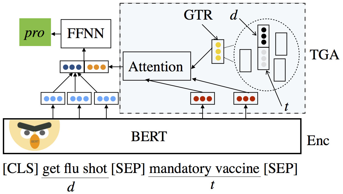
Figure 1: Architecture of TGA Net. Enc indicates contextual conditional encoding (§4.2), GTR indicates Generalized Topic Representation (§4.3), TGA indicates Topic-grouped Attention (4.4).

4 Methods

We develop Topic-Grouped Attention (TGA) Net: a model to implicitly construct and use relationships between the training and evaluation topics without supervision. The model consists of a contextual conditional encoding layer (§4.2), followed by topic-grouped attention (§4.4) using generalized topic representations (§4.3) and a feed-forward neural network (see Figure 1).

4.1 Definitions

Let $D=\{x_{i}=(d_{i},t_{i},y_{i})\}_{i=1}^{N}$ be a dataset with $N$ examples, each consisting of a document $d_{i}$ (a comment), a topic $t_{i}$, and a stance label $y_{i}$. Recall that for each unique document $d$, the data may contain examples with different topics. For example (1) and (2) (Table 2) have the same document but different topics. The task is to predict a stance label $\hat{y}\in\{\text{pro, con, neutral}\}$ for each $x_{i}$, based on the topic-phrase definition of stance (see §2).

4.2 Contextual Conditional Encoding

Since computing the stance of a document is dependent on the topic, prior methods for cross-target stance have found that bidirectional conditional encoding (conditioning the document representation on the topic) provides large improvements (Augenstein et al., 2016). However, prior work used static word embeddings and we want to take advantage of contextual emebddings. Therefore, we embed a document and topic jointly using BERT (Devlin et al., 2019). That is, we treat the document and topic as a sentence pair, and obtain two sequences of token embeddings $\bar{t}=t^{(1)},\ldots,t^{(m)}$ for the topic $t$ and $\bar{d}=d^{(1)},\ldots,d^{(n)}$ for the document $d$. As a result, the text embeddings are implicitly conditioned on the topic, and vice versa.

4.3 Generalized Topic Representations (GTR)

For each example $x=(d,t,y)$ in the data, we compute a generalized topic representation $r_{dt}$: the centroid of the nearest cluster to $x$ in euclidean space, after clustering the training data. We use hierarchical clustering on $v_{dt}=[v_{d};v_{t}]$, a representation of the document $d$ and text $t$, to obtain clusters. We use one $v_{d}\in\mathbb{R}^{E}$ and one $v_{t}\in\mathbb{R}^{E}$ (where $E$ is the embedding dimension) for each unique document $d$ and unique topic $t$.

To obtain $v_{d}$ and $v_{t}$, we first embed the document and topic separately using BERT (i.e., [CLS] $<$text$>$ [SEP] and [CLS] $<$topic$>$ [SEP]) then compute a weighted average over the token embeddings $\bar{d}$ (and similarly $\bar{t}$). In this way, $v_{d}$ ($v_{t}$) is independent of all topics (comments) and so $v_{d}$ and $v_{t}$ can share information across examples. That is, for examples $x_{i},x_{j},x_{k}\in D$ we may have that $d_{i}=d_{j}$ but $d_{j}\neq d_{k}$ and $t_{j}=t_{k}$ but $t_{i}\neq t_{j}$. The token embeddings are weighted in $v_{d}$ by tf-idf, in order to downplay the impact of common content words (e.g., pronouns or adverbs) in the average. In $v_{t}$, the token embeddings are weighted uniformly.

4.4 Topic-Grouped Attention

We use the generalized topic representation $r_{dt}$ for example $x$ to compute the similarity between $t$ and other topics in the dataset. Using learned scaled dot-product attention (Vaswani et al., 2017), we compute similarity scores $s_{i}$ and use these to weigh the importance of the current topic tokens $t^{(i)}$, obtaining a representation $c_{dt}$ that captures the relationship between $t$ and related topics and documents. That is, we compute

$$c_{dt}=\sum_{i}s_{i}t^{(i)},\ s_{i}=\text{softmax}\Big{(}\lambda t^{(i)}\cdot(W_{a}r_{dt})\Big{)}$$

where $W_{a}\in\mathbb{R}^{E\times 2E}$ are learned parameters and $\lambda=1/\sqrt{E}$ is the scaling value.

4.5 Label Prediction

To predict the stance label, we combine the output of our topic-grouped attention with the document token embeddings and pass the result through a feed-forward neural network to compute the output probabilities $p\in\mathbb{R}^{3}$. That is,

$$p=\text{softmax}(W_{2}(\tanh(W_{1}[\tilde{d};c_{dt}]+b_{1})+b_{2}))$$

where $\tilde{d}=\frac{1}{n}\sum_{i}d^{(i)}$ and $W_{1}\in\mathbb{R}^{h\times 2E},W_{2}\in\mathbb{R}^{3\times h},b_{1}\in\mathbb{R}^{h},b_{2}\in\mathbb{R}^{3}$ are learned parameters and $h$ is the hidden size of the network. We minimize cross-entropy loss.

	Train	Dev	Test
# Examples	13477	2062	3006
# Unique Comments	1845	682	786
# Few-shot Topics	638	114	159
# Zero-shot Topics	4003	383	600

Table 4: Data split statistics for VAST.

5 Experiments

5.1 Data

We split VAST such that all examples $x_{i}=(d_{i},t_{i},y_{i})$ where $d_{i}=d$, for a particular document $d$, are in exactly one partition. That is, we randomly assign each unique $d$ to one partition of the data. We assign $70\%$ of unique documents to the training set and split the remainder evenly between development and test. In the development and test sets we only include examples of types Heur and Corr (we exclude all noisy List examples).

We create separate zero-shot and few-shot development and test sets. The zero-shot development and test sets consist of topics (and documents) that are not in the training set. The few-shot development and test sets consist of topics in the training set (see Table 4). For example, there are $600$ unique topics in the zero-shot test set (none of which are in the training set) and $159$ unique topics in the few-shot test set (which are in the training set). This design ensures that there is no overlap of topics between the training set and the zero-shot development and test sets both for pro/con and neutral examples. We preprocess the data by tokenizing and removing stopwords and punctuation using NLTK.

Due to the linguistic variation in the topic expressions (§3.2), we examine the prevalence of lexically similar topics, LexSimTopics, (e.g., ‘taxation policy’ vs. ‘tax policy’) between the training and zero-shot test sets. Specifically, we represent each topic in the zero-shot test set and the training set using pre-trained GloVe (Pennington et al., 2014) word embeddings. Then, test topic $t_{i}^{(t)}$ is a LexSimTopic if there is at least one training topic $t_{j}^{(r)}$ such that $\text{cosine}\_\text{sim}(t_{i}^{(t)},t_{j}^{(r)})\geq\theta$ for fixed $\theta\in\mathbb{R}$. We manually examine a random sample of zero-shot dev topics to determine an appropriate threshold $\theta$. Using the manually determined threshold $\theta=0.9$, we find that only $16\%$ ($96$ unique topics) of the topics in the entire zero-shot test set are LexSimTopics.

5.2 Baselines and Models

We experiment with the following models:

• CMaj: the majority class computed from each cluster in the training data.

• BoWV: we construct separate BoW vectors for the text and topic and pass their concatenation to a logistic regression classifier.

• C-FFNN: a feed-forward network trained on the generalized topic representations.

• BiCond: a model for cross-target stance that uses bidirectional encoding, whereby the topic is encoded using a BiLSTM as $h_{t}$ and the text is then encoded using a second BiLSTM conditioned on $h_{t}$ (Augenstein et al., 2016). This model uses fixed pre-trained word embeddings. A weakly supervised version of BiCond is currently state-of-the-art on cross-target TwitterStance.

• CrossNet: a model for cross-target stance that encodes the text and topic using the same bidirectional encoding as BiCond and adds an aspect-specific attention layer before classification (Xu et al., 2018). Cross-Net improves over BiCond in many cross-target settings.

• BERT-sep: encodes the text and topic separately, using BERT, and then classification with a two-layer feed-forward neural network.

• BERT-joint: contextual conditional encoding followed by a two-layer feed-forward neural network.

• TGA Net: our model using contextual conditional encoding and topic-grouped attention.

5.2.1 Hyperparameters

We tune all models using uniform hyperparameter sampling on the development set. All models are optimized using Adam (Kingma and Ba, 2015), maximum text length of $200$ tokens (since $<5\%$ of documents are longer) and maximum topic length of $5$ tokens. Excess tokens are discarded

For BoWV we use all topic words and a comment vocabulary of $10,000$ words. We optimize using using L-BFGS and L2 penalty. For BiCond and Cross-Net we use fixed pre-trained $100$ dimensional GloVe (Pennington et al., 2014) embeddings and train for $50$ epochs with early stopping on the development set. For BERT-based models, we fix BERT, train for $20$ epochs with early stopping and use a learning rate of $0.001$. We include complete hyperparameter information in Appendix A.1.1.

We cluster generalized topic representations using Ward hierarchical clustering (Ward, 1963), which minimizes the sum of squared distances within a cluster while allowing for variable sized clusters. To select the optimal number of clusters $k$, we randomly sample $20$ values for $k$ in the range $[50,300]$ and minimize the sum of squared distances for cluster assignments in the development set. We select $197$ as the optimal $k$.

	F1 All			F1 Zero-Shot			F1 Few-Shot
	pro	con	all	pro	con	all	pro	con	all
CMaj	.382	.441	.274	.389	.469	.286	.375	.413	.263
BoWV	.457	.402	.372	.429	.409	.349	.486	.395	.393
C-FFNN	.410	.434	.300	.408	.463	.417	.413	.405	.282
BiCond	.469	.470	.415	.446	.474	.428	.489	.466	.400
Cross-Net	.486	.471	.455	.462	.434	.434	.508	.505	.474
BERT-sep	.4734	.522	.5014	.414	.506	.454	.524	.539	.544
BERT-joint	.545	.591	.653	.546	.584	.661	.544	.597	.646
TGA Net	.573*	.590	.665	.554	.585	.666	.589*	.595	.663

Table 5: Macro-averaged F1 on the test set. ^∗ indicates significance of TGA Net over BERT-joint, $p<0.05$.

5.3 Results

Test Topic	Cluster Topics
drug addicts	war drug, cannabis, legalization, marijuana popularity, social effect, pot, colorado, american lower class, gateway drug, addiction, smoking marijauana, social drug
oil drilling	natural resource, international cooperation, renewable energy, alternative energy, petroleum age, electric car, solar use, offshore drilling, offshore exploration, planet
free college education	tax break home schooling, public school system, education tax, funding education, public service, school tax, homeschool tax credit, community, home schooling parent

Table 6: Topics from test examples and training examples in their assigned cluster.

We evaluate our models using macro-average F1 calculated on three subsets of VAST (see Table 5): all topics, topics only in the test data (zero-shot), and topics in the train or development sets (few-shot). We do this because we want models that perform well on both zero-shot topics and training/development topics.

We first observe that CMaj and BoWV are strong baselines for zero-shot topics. Next, we observe that BiCond and Cross-Net both perform poorly on our data. Although these were designed for cross-target stance, a more limited version of zero-shot stance, they suffer in their ability to generalize across a large number of targets when few examples are available for each.

We see that while TGA Net and BERT-joint are statistically indistinguishable on all topics, the topic-grouped attention provides a statistically significant improvement for few-shot learning on ‘pro’ examples (with $p<0.05$). Note that conditional encoding is a crucial part of the model, as this provides a large improvement over embedding the comment and topic separately (BERT-sep).

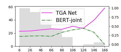
Figure 2: Percentage (right y-axis) each model is best on the test set as a function of the number of unique topics in each cluster. Histogram (left y-axis) of unique topics shown in gray.

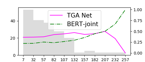
Figure 3: Percentage (right y-axis) each model is best on the test set as a function of the number of examples per cluster. Histogram of cluster sizes (left y-axis) shown in gray.

Additionally, we compare the performance of TGA Net and BERT-joint on both zero-shot LexSimTopics and non-LexSimTopics. We find that while both models exhibit higher performance on zero-shot LexSimTopics ($.70$ and $.72$ F1 respectively), these topics are such a small fraction of the zero-shot test topics that zero-shot evaluation primarily reflects model performance on the non-LexSimTopics. Additionally, the difference between performance on zero-shot LexSimTopics and non-LexSimTopics is less for TGA Net (only $0.04$ F1) than for BERT-joint ($0.06$ F1), showing our model is better able to generalize to lexically distinct topics.

To better understand the effect of topic-grouped attention, we examine the clusters generated in §4.3 (see Table 6). The clusters range in size from $7$ to $257$ examples (median $62$) with the number of unique topics per cluster ranging from $6$ to $166$ (median $43$). We see that the generalized representations are able to capture relationships between zero-shot test topics and training topics.

		Imp	mlT	mlS	Qte	Sarc
BERT joint	I	.600	.610	.541	.625	.587
	O	.710	.748	.713	.657	.662
TGA Net	I	.623	.624	.547	.661	.637
	O	.713	.752	.725	.663	.667

Table 7: Accuracy on varying phenomena in the test set. I indicates examples with the phenomenon, O indicates examples without.

Comment	Topic	$\mathcal{\ell}$
… we need(-) to get those GOP members out of the House & Senate, since they only support(+)$\rightarrow$ patronize(-) billionaire tax breaks, evidently(+)$\rightarrow$ obviously(-). We need(-) MORE PARKS. And they should all be FREE(+)$\rightarrow$ gratuitous(-) …	government spending on parks	Pro
… debaters don’t strike(-)$\rightarrow$ shine(+) me as being anywhere near diverse in their perspectives on guns. Not one of the gun-gang cited any example of where a student with a gun saved someone from something terrible(-) $\rightarrow$ tremendous(+) on their campuses. At least(-) the professor speaks up for rationality(+).	guns	Con

Table 8: Examples with changed majority sentiment polarity. Sentiment words are bold italicized, for removed words (struck out) and positive ( green (+)) and negative ( red (-)) sentiment words.

		BERT joint	TGA Net
Pro	$M+$	.73	.77
	$M-$	.65	.68
	$M+\rightarrow M-$ ($\downarrow$)	.71$\rightarrow$.69	.74$\rightarrow$.67
	$M-\rightarrow M+$ ($\uparrow$)	.71$\rightarrow$.74	.71$\rightarrow$.70
Con	$M+$	.74	.70
	$M-$	.79	.80
	$M+\rightarrow M-$ ($\uparrow$)	.76$\rightarrow$.80	.70$\rightarrow$.74
	$M-\rightarrow M+$ ($\downarrow$)	.75$\rightarrow$.71	.75$\rightarrow$.74

Table 9: F1 on the test set for examples with a majority sentiment polarity ($M$) and conversion between sentiment polarities (e.g., $M+\rightarrow M-$). The direction the score a sentiment-susceptible model is expected to change is indicated with $\uparrow$ or $\downarrow$.

We also evaluate the percentage of times each of our best performing models (BERT-joint and TGA Net) is the best performing model on a cluster as a function of the number of unique topics (Figure 2) and cluster size (Figure 3). To smooth outliers, we first bin the cluster statistic and calculate each percent for clusters with at least that value (e.g., clusters with at least $82$ examples). We see that as the number of topics per cluster increases, TGA Net increasingly outperforms BERT-joint. This shows that the model is able to benefit from diverse numbers of topics being represented in the same manner. On the other hand, when the number of examples per cluster becomes too large ($>182$), TGA NET’s performance suffers. This suggests that when cluster size is very large, the stance signal within a cluster becomes too diverse for topic-grouped attention to use.

5.4 Error Analysis

5.4.1 Challenging Phenomena

We examine the performance of TGA Net and BERT-joint on five challenging phenomena in the data: i) Imp – the topic phrase is not contained in the document and the label is not neutral ($1231$ cases), ii) mlT – a document is in examples with multiple topics ($1802$ cases), iii) mlS – a document is in examples with different, non-neutral, stance labels (as in (3) and (4) Table 2) ($952$ cases), iv) Qte – a document with quotations, and v) Sarc – sarcasm, as annotated by Habernal et al. (2018).

We choose these phenomena to cover a range of challenges for the model. First, Imp examples require the model to recognize concepts related to the unmentioned topic in the document (e.g., recognizing that computers are related to the topic ‘3d printing’). Second, to do well on mlT and mlS examples, the model must learn more than global topic-to-stance or document-to-stance patterns (e.g., it cannot predict a single stance label for all examples with a particular document). Finally, quotes are challenging because they may repeat text with the opposite stance to what the author expresses themselves (see Appendix Table 20 for examples).

Overall, we find the TGA Net performs better on these difficult phenomena (see Table 7). These phenomena are challenging for both models, as indicated by the generally lower performance on examples with the phenomena compared to those without, with the mlS especially difficult. We observe that TGA Net has particularly large improvements on the rhetorical devices (Qte and Sarc), suggesting that topic-grouped attention allows the model to learn more complex semantic information in the documents.

5.4.2 Stance and Sentiment

Finally, we investigate the connection between stance and sentiment vocabulary. Specifically, we use the MPQA sentiment lexicon (Wilson et al., 2017) to identify positive and negative sentiment words in texts. We observe that in the test set, the majority ($80\%$) of pro examples have more positive than negative sentiment words, while only $41\%$ of con examples have more negative than positive sentiment words. That is, con stance is often expressed using positive sentiment words but pro stance is rarely expressed using negative sentiment words and therefore there is not a direct mapping between sentiment and stance.

We use $M+$ to denote majority positive sentiment polarity and similarity for $M-$ and negative. We find that on pro examples with $M-$, TGA Net outperforms BERT-joint, while the reverse is true for con examples with $M+$. For both stance labels and models, performance increases when the majority sentiment polarity agrees with the stance label ($M+$ for pro, $M-$ for con). Therefore, we investigate how susceptible both models are to changes in sentiment.

To test model susceptibility to sentiment polarity, we generate swapped examples. For examples with majority polarity $p$, we randomly replace sentiment words with a WordNet synonym of opposite polarity until the majority polarity for the example is $-p$ (see Table 8). We then evaluate our models on the examples before and after the replacements.

When examples are changed from the opposite polarity ($-\rightarrow+$ for pro, $+\rightarrow-$ for con), a model that relies too heavily on sentiment should increase performance. Conversely, when converting to the opposite polarity ($+\rightarrow-$ for pro, $-\rightarrow+$ for con) an overly reliant model’s performance should decrease. Although the examples contain noise, we find that both models are reliant on sentiment cues, particularly when adding negative sentiment words to a pro stance text. This suggests the models are learning strong associations between negative sentiment and con stance.

Our results also show TGA Net is less susceptible to replacements than BERT-joint. On pro $-\rightarrow+$, performance actually decreases by one point (BERT-joint increases by three points) and on con $-\rightarrow+$ performance only decreases by one point (compared to four for BERT-joint). TGA Net is better able to distinguish when positive sentiment words are actually indicative of a pro stance, which may contribute to its significantly higher performance on pro. Overall, TGA Net relies less on sentiment cues than other models.

6 Conclusion

We find that our model TGA Net, which uses generalized topic representations to implicitly capture relationships between topics, performs significantly better than BERT for stance detection on pro labels, and performs similarly on other labels. In addition, extensive analysis shows our model provides substantial improvement on a number of challenging phenomena (e.g., sarcasm) and is less reliant on sentiment cues that tend to mislead the models. Our models are evaluated on a new dataset, VAST, that has a large number of topics with wide linguistic variation and that we create and make available.

In future work we plan to investigate additional methods to represent and use generalized topic information, such as topic modeling. In addition, we will study more explicitly how to decouple stance models from sentiment, and how to improve performance further on difficult phenomena.

7 Acknowledgements

We thank the Columbia NLP group and the anonymous reviewers for their comments. This work is based on research sponsored by DARPA under agreement number FA8750-18- 2-0014. The U.S. Government is authorized to reproduce and distribute reprints for Governmental purposes notwithstanding any copyright notation thereon. The views and conclusions contained herein are those of the authors and should not be interpreted as necessarily representing the official policies or endorsements, either expressed or implied, of DARPA or the U.S. Government.

Appendix A Appendices

A.0.1 Crowdsourcing

We show a snap shot of one ‘HIT’ of the data annotation task in Figure 4. We paid annotators $\$0.13$ per HIT. We had a total of $696$, of which we removed $183$ as a result of quality control.

A.0.2 Data

We show complete examples from the dataset in Table 10. These show the topics extracted from the original ARC stance position, potential annotations and corrections, and the topics listed by annotators as relevant to each comment.

In (a), (d), (i), (j), and (l) the topic make sense to take a position on (based on the comment) and annotators do not correct the topics and provide a stance label for that topic directly. In contrast, the annotators correct the provided topics in (b), (c), (e), (f), (g), (h), and (k). The corrections are because the topic is not possible to take a position on (e.g., ‘trouble’), or not specific enough (e.g, ‘california’, ‘a tax break’). In one instance, we can see that one annotator chose to correct the topic (k) whereas another annotator for the same topic and comment chose not to (j). This shows how complex the process of stance annotation is.

We also can see from the examples the variations in how similar topics are expressed (e.g., ‘public education’ vs. ‘public schools’) and the relationship between the stance label assigned for the extracted (or corrected topic) and the listed topic. In most instances, the same label applies to the listed topics. However, we show two instances where this is not the case: (d) – the comment actually supports ‘public schools’ and (i) – the comment is actually against ‘airline’). This shows that this type of example (ListTopic, see §3.1.2), although somewhat noisy, is generally correctly labeled using the provided annotations.

We also show neutral examples from the dataset in Table 11. Examples 1 and 2 were constructed using the process described in §3.1.3. We can see that the new topics are distinct from the semantic content of the comment. Example 3 shows an annotator provided neutral label since the comment is neither in support of or against the topic ‘women’s colleges’. This type of neutral example is less common than the other (in 1 and 2) and is harder, since the comment is semantically related to the topic.

A.1 Experiments

A.1.1 Hyperparameters

All neural models are implemented in Pytorch and tuned on the developement. Our logistic regression model is implemented with scikit-learn. The number of trials and training time are shown in Table 12. Hyperparameters are selected through uniform sampling. We also show the hyperparameter search space and best configuration for C-FFNN (Table 13), BiCond (Table 14), Cross-Net (Table 15), BERT-sep (Table 16), BERT-joint (Table 17) and TGA Net (Table 18). We use one TITAN Xp GPU.

We calculate expected validation performance (Dodge et al., 2019) for F1 in all three cases and additionally show the performance of the best model on the development set (Tale 19). Models are tuned on the development set and we use macro-averaged F1 of all classes for zero-shot examples to select the best hyperparameter configuration for each model. We use the scikit-learn implementation of F1. We see that the improvement of TGA Net over BERT-joint is high on the development set.

A.1.2 Results

A.1.3 Error Analysis

We investigate the performance of our two best models (TGA Net and BERT-joint) on five challenging phenomena, as discussed in §5.4.1. The phenomena are:

• Implicit (Imp): the topic is not contained in the document.

• Multiple Topics (mlT): document has more than one topic.

• Multiple Stance (mlS): a document has examples with different, non-neutral, stance labels.

• Quote (Qte): the document contains quotations.

• Sarcasm (Sarc): the document contains sarcasm, as annotated by Habernal et al. (2018).

We show examples of each of these phenomena in Table 20.

A.1.4 Stance and Sentiment

To construct examples with swapped sentiment words we use the MPQA lexicon (Wilson et al., 2017) for sentiment words. We use WordNet to select synonyms with opposite polarity, ignoring word sense and part of speech. We show examples from each set type of swap, $+\rightarrow-$ (Table 22) and $-\rightarrow+$ (Table 21). In total there are $1158$ positive sentiment words and $1727$ negative sentiment words from the lexicon in our data. Of these, $218$ positive words have synonyms with negative sentiment, and $224$ negative words have synonyms with positive sentiment.

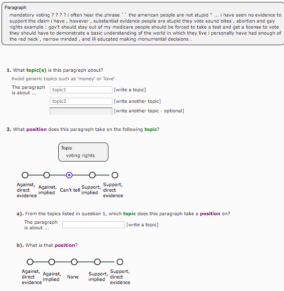
Figure 4: Snapshot of Amazon Mechanical Turk Annotation Task with sample input data.

Comment	ARC Stance	Extracted Topic	Listed Topic	$\mathcal{\ell}$
So based on these numbers London is forking out  12-24 Billion dollars to pay for the Olympics. According to the Official projection they have already spent 12 Billion pounds (or just abous $20 billion). Unofficially the bill is looking more like 24 Billion pounds (or closer to 40 Billion dollars). What a complete waste of Money.	Olympics are more trouble	•olympics	•olympics	C	a
			•london olympics budget
3-6		trouble $\Rsh$ •spending	•wasting money	C	b
		money on the olympics	•sport
3-6		trouble $\Rsh$ •olympics	• london finances	C	c
The era when there were no public schools was not a good socio-economic time in the life of our nation. Anything which weakens public schools and their funding will result in the most vulnerable youth of America being left out of the chance to get an education.	Home schoolers do not deserve a tax break	•home schoolers	• public schools	C	d
3-6		a tax break $\Rsh$ •public schools	•youth of america	P	e
3-6		a tax break $\Rsh$ •public education	•public education funding	P	f
Airports and the roads on east nor west coast can not handle the present volume adequately as is. I did ride the vast trains in Europe, Japan and China and found them very comfortable and providing much better connections and more efficient.	California needs high-speed rail	california $\Rsh$ •train	•transportation	P	g
3-6		california $\Rsh$ •traffic	•roadway	C	h
3-6		•high-speed rail	•airline •public transit	P	i
There is only a shortage of agricultural labor at current wages. Raise the wage to a fair one, and legal workers will do it. If US agriculture is unsustainable without abusive labor practices, should we continue to prop up those practices?	Farms could survive without illegal labor	•farms	• agricultural labor	C	j
3-6		farms $\Rsh$ •illegal workers	•agricultural labor wages	C	k
3-6		•illegal labor	•agricultural labor •labor	C	l

Table 10: Complete examples from our dataset with extracted topics ( green, italic) and corrections (old struck out). Topics related to the comment are also shown (listed topics), as are labels ($\mathcal{\ell}$), where P indicates Pro and C indicates C. Each label applies to all topics in the cell. Phrases related to the corrections or listed topics are highlighted in yellow.

Comment	Original Topic	$\mathcal{\ell}$	New Topic
Good idea. I have always had a cat or two. While being inhumane, declawing places a cat in danger. Should my charming indoor kitty somehow escape outside, he would have no way to defend himself.Why don’t humans have their finger-and tonails removed to save on manicures? Answer:they are important to the functioning and protection of our bodies.	nail removal	Pro	attack	1
Marijuana is not addictive – and is much less dangerous than alcohol. The gate-way drugs are prescription meds found in medicine cabinets everywhere. Heroin is a lot less expensive than marijuana and if marijuana were legal, and less expensive, fewer people would want heroin.	prescription meds	Con	israel	2
There are no women only law schools. Womens’ colleges, like Mills College, that do offer graduate degrees have co-ed graduate schools. The example of Hillary Clinton’s success at Yale Law School either says nothing about womens’ colleges or supports them.	women’s colleges	N	women’s colleges	3

Table 11: Neutral examples from the dataset. N indicates neutral original label

	TGA Net	BERT-joint	BERT-sep	BiCond	Cross-Net	C-FFNN
# search trials	10	10	10	20	20	20
Training time (seconds)	6550.2	2032.2	1995.6	2268.0	2419.8	5760.0
# Parameters	617543	435820	974820	225108	205384	777703

Table 12: Search time and trials for various models.

Hyperparameter	Search space	Best Assignment
batch size	64	64
epochs	50	50
dropout	uniform-float[$0.1,0.3$]	$0.28149172466319095$
hidden size	uniform-integer[$300,1000$]	$505$
learning rate	$0.001$	$0.001$
learning rate optimizer	Adam	Adam

Table 13: Hyperparameter search space and setting for C-FFNN.

Hyperparameter	Search space	Best Assignment
batch size	64	64
epochs	100	100
dropout	uniform-float[$0.1,0.5$]	$04850254141775727$
hidden size	uniform-integer[$40,100$]	$78$
learning rate	loguniform[$0.001,0.01$]	$0.004514020306243207$
learning rate optimizer	Adam	Adam
pre-trained vectors	Glove	Glove
pre-trained vector dimension	100	100

Table 14: Hyperparameter search space and setting for BiCond.

Hyperparameter	Search space	Best Assignment
batch size	64	64
epochs	100	100
dropout	uniform-float[$0.1,0.5$]	$0.36954545196802335$
BiLSTM hidden size	uniform-integer[$40,100$]	$68$
linear layer hidden size	uniform-integer[$20,60$]	$48$
attention hidden size	uniform-integer[$20,100$]	$100$
learning rate	loguniform[$0.001,0.01$]	$0.00118168557993075$
learning rate optimizer	Adam	Adam
pre-trained vectors	Glove	Glove
pre-trained vector dimension	100	100

Table 15: Hyperparameter search space and setting for Cross-Net.

Hyperparameter	Search space	Best Assignment
batch size	$64$	$64$
epochs	$20$	$20$
dropout	uniform-float[$0.1,0.3$]	$0.22139772968435562$
hidden size	uniform-integer[$300,1000$]	$633$
learning rate	$0.001$	$0.001$
learning rate optimizer	Adam	Adam

Table 16: Hyperparameter search space and setting for BERT-sep.

Hyperparameter	Search space	Best Assignment
batch size	64	64
epochs	20	20
dropout	uniform-float[$0.1,0.4$]	$0.20463604390811982$
hidden size	uniform-integer[$200,800$]	$283$
learning rate	$0.001$	$0.001$
learning rate optimizer	Adam	Adam

Table 17: Hyperparameter search space and setting for BERT-joint.

Hyperparameter	Search space	Best Assignment
batch size	$64$	$64$
epochs	$50$	$50$
dropout	uniform-float[$0.1,0.3$]	$0.35000706311476193$
hidden size	uniform-integer[$300,1000$]	$401$
learning rate	$0.001$	$0.001$
learning rate optimizer	Adam	Adam

Table 18: Hyperparameter search space and settings for TGA Net.

	Best Dev			$\mathbb{E}$[Dev]
	F1a	F1z	F1f	F1a	F1z	F1f
CMaj	.3817	.2504	.2910	–	–	–
BoWV	.3367	.3213	.3493	–	–	–
C-FFNN	.3307	.3147	.3464	.3315	.3128	.3590
BiCond	.4229	.4272	.4170	.4423	.4255	.4760
Cross-Net	.4779	.4601	.4942	.4751	.4580	.4979
BERT-sep	.5314	.5109	.5490	.5308	.5097	.5519
BERT-joint	.6589	.6375	.6099	.6579	.6573	.6566
TGA Net	.6657	.6851	.6421	.6642	.6778	.6611

Table 19: Best results on the development set and expected validation score (Dodge et al., 2019) for all tuned models. $a$ is All, $z$ is zero-shot, $f$ is few-shot.

Type	Comment	Topic	$\mathcal{\ell}$
Imp	No, it’s not just that the corporations will have larger printers. It is that most of us will have various sizes of printers. IT’s just what happened with computers. I was sold when some students from Equador showed me their easy to make, working, prosthetic arm. Cost to make, less than one hundred dollars.	•3d printing	Pro
Sarc	yes, let’s hate cyclists: people who get off their ass and ride, staying fit as they get around the city. they don’t pollute the air, they don’t create noise, they don’t create street after street clogged with cars dripping oil… I think the people who hate cyclists are the same ones who hate dogs: they have tiny little shards of coal where their heart once was. they can’t move fast or laugh, and want no one else to, either. According to the DMV, in 2009 there were 75,539 automobile crashes in New York City, less than 4 percent of those crashes involved a bicycle. cyclists are clearly the problem here.	•cyclists	Pro
Qte	“cunning, baffling and powerful disease of addiction” - LOL no. This is called ’demon possession’. Let people do drugs. They’ll go through a phase and then they’ll get tired of it and then they’ll be fine. UNLESS they end up in treatment and must confess a disease of free will, in which case all bets are off.	• disease of addiction	Con
mlS	That this is even being debated is evidence of the descent of American society into madness. The appalling number of gun deaths in America is evidence that more guns would make society safer? Only in the US does this kind of logic translate into political or legal policy. I guess that’s what exceptionalism means.	•guns •gun control	Con Pro
mlT	The focus on tenure is just another simplistic approach to changing our educational system. The judge also overlooked that tenure can help attract teachers. Living in West Virginia, a state with many small and isolated communities, why would any teacher without personal ties to our state come here, if she can fired at will? I know that I and my wife would not.	•tenure •stability	Pro Pro

Table 20: Examples of hard phenomena in the dataset as discussed in §5.4.1.

Negative(-) Word	Positive(+) Word
inevitably	necessarily
low	humble
resistant	tolerant
awful	tremendous
eliminate	obviate
redundant	spare
rid	free
hunger	crave
exposed	open
mad	excited
indifferent	unbiased
denial	defense
costly	dear
weak	light
laughable	amusing
worry	interest
pretend	profess
depression	impression
fight	press
trick	joke
slow	easy
sheer	bold
doom	destine
wild	fantastic
laugh	jest
partisan	enthusiast
deep	rich
restricted	qualified
gamble	adventure
shake	excite
scheme	dodge
suffering	brook
burn	glow
argue	reason
oppose	defend
hard	strong
complicated	refine
fell	settle
avoid	obviate
hedge	dodge

Table 21: Example word pairs for converting words from negative(-) to positive(+) sentiment.

Positive(+) Word	Negative(-) Word
compassion	pity
terrified	terrorize
frank	blunt
modest	low
magic	illusion
sustained	suffer
astounding	staggering
adventure	gamble
glow	burn
spirited	game
enduring	suffer
wink	flash
sincere	solemn
amazing	awful
triumph	wallow
compassionate	pity
plain	obviously
stimulating	shake
excited	mad
sworn	swear
unbiased	indifferent
compelling	compel
exciting	shake
yearn	ache
validity	rigor
seasoned	temper
appealing	sympathetic
innocent	devoid
pure	stark
super	extremely
interesting	worry
productive	fat
strong	stiff
fortune	hazard
rally	bait
motivation	need
ultra	radical
justify	rationalize
amusing	laughable
awe	fear

Table 22: Example word pairs for converting words from positive(+) to negative(-) sentiment.

References

- Abbott et al. (2016) Rob Abbott, Brian Ecker, Pranav Anand, and Marilyn A. Walker. 2016. Internet argument corpus 2.0: An sql schema for dialogic social media and the corpora to go with it. In LREC.
- Augenstein et al. (2016) Isabelle Augenstein, Tim Rocktäschel, Andreas Vlachos, and Kalina Bontcheva. 2016. Stance detection with bidirectional conditional encoding. In EMNLP.
- Bar-Haim et al. (2017) Roy Bar-Haim, Indrajit Bhattacharya, Francesco Dinuzzo, Amrita Saha, and N. Slonim. 2017. Stance classification of context-dependent claims. In EACL.
- Beigman Klebanov et al. (2010) Beata Beigman Klebanov, Eyal Beigman, and Daniel Diermeier. 2010. Vocabulary choice as an indicator of perspective. In Proceedings of the ACL 2010 Conference Short Papers, pages 253–257, Uppsala, Sweden. Association for Computational Linguistics.
- Devlin et al. (2019) Jacob Devlin, Ming-Wei Chang, Kenton Lee, and Kristina Toutanova. 2019. Bert: Pre-training of deep bidirectional transformers for language understanding. ArXiv, abs/1810.04805.
- Dias and Becker (2016) Marcelo Dias and Karin Becker. 2016. Inf-ufrgs-opinion-mining at semeval-2016 task 6: Automatic generation of a training corpus for unsupervised identification of stance in tweets. In SemEval@NAACL-HLT.
- Dodge et al. (2019) Jesse Dodge, Suchin Gururangan, Dallas Card, Roy Schwartz, and Noah A. Smith. 2019. Show your work: Improved reporting of experimental results. In EMNLP/IJCNLP.
- Du et al. (2017) Jiachen Du, Ruifeng Xu, Yulan He, and Lin Gui. 2017. Stance classification with target-specific neural attention. In IJCAI.
- Faulkner (2014) Adam Faulkner. 2014. Automated classification of stance in student essays: An approach using stance target information and the wikipedia link-based measure. In FLAIRS Conference.
- Ferreira and Vlachos (2016) William Ferreira and Andreas Vlachos. 2016. Emergent: a novel data-set for stance classification. In HLT-NAACL.
- Gottipati et al. (2013) Swapna Gottipati, Minghui Qiu, Yanchuan Sim, Jing Jiang, and Noah A. Smith. 2013. Learning topics and positions from debatepedia. In EMNLP.
- Habernal et al. (2018) Ivan Habernal, Henning Wachsmuth, Iryna Gurevych, and Benno Stein. 2018. The argument reasoning comprehension task: Identification and reconstruction of implicit warrants. In NAACL-HLT.
- Hasan and Ng (2013) Kazi Saidul Hasan and Vincent Ng. 2013. Stance classification of ideological debates: Data, models, features, and constraints. In IJCNLP.
- Hasan and Ng (2014) Kazi Saidul Hasan and Vincent Ng. 2014. Why are you taking this stance? identifying and classifying reasons in ideological debates. In EMNLP.
- Hovy et al. (2013) Dirk Hovy, Taylor Berg-Kirkpatrick, Ashish Vaswani, and Eduard H. Hovy. 2013. Learning whom to trust with mace. In HLT-NAACL.
- Kingma and Ba (2015) Diederik P. Kingma and Jimmy Ba. 2015. Adam: A method for stochastic optimization. CoRR, abs/1412.6980.
- Krejzl et al. (2017) Peter Krejzl, Barbora Hourová, and Josef Steinberger. 2017. Stance detection in online discussions. ArXiv, abs/1701.00504.
- Küçük (2017) Dilek Küçük. 2017. Stance detection in turkish tweets. ArXiv, abs/1706.06894.
- Küçük and Can (2020) Dilek Küçük and F. Can. 2020. Stance detection: A survey. ACM Computing Surveys (CSUR), 53:1 – 37.
- Li et al. (2018) Chang Li, Aldo Porco, and Dan Goldwasser. 2018. Structured representation learning for online debate stance prediction. In COLING.
- Lin et al. (2006) Wei-Hao Lin, Theresa Wilson, Janyce Wiebe, and Alexander G. Hauptmann. 2006. Which side are you on? identifying perspectives at the document and sentence levels. In CoNLL.
- Lozhnikov et al. (2018) Nikita Lozhnikov, Leon Derczynski, and Manuel Mazzara. 2018. Stance prediction for russian: Data and analysis. ArXiv, abs/1809.01574.
- Mohammad et al. (2016) Saif M. Mohammad, Svetlana Kiritchenko, Parinaz Sobhani, Xiao-Dan Zhu, and Colin Cherry. 2016. Semeval-2016 task 6: Detecting stance in tweets. In SemEval@NAACL-HLT.
- Mohammad et al. (2017) Saif M. Mohammad, Parinaz Sobhani, and Svetlana Kiritchenko. 2017. Stance and sentiment in tweets. ACM Trans. Internet Techn., 17:26:1–26:23.
- Murakami and Putra (2010) Akiko Murakami and Raymond H. Putra. 2010. Support or oppose? classifying positions in online debates from reply activities and opinion expressions. In COLING.
- Pennington et al. (2014) Jeffrey Pennington, Richard Socher, and Christopher D. Manning. 2014. Glove: Global vectors for word representation. In Empirical Methods in Natural Language Processing (EMNLP), pages 1532–1543.
- Somasundaran and Wiebe (2010) Swapna Somasundaran and Janyce Wiebe. 2010. Recognizing stances in ideological on-line debates. In HLT-NAACL 2010.
- Sridhar et al. (2015) Dhanya Sridhar, James Foulds, Bert Huang, Lise Getoor, and Marilyn Walker. 2015. Joint models of disagreement and stance in online debate. In Proceedings of the 53rd Annual Meeting of the Association for Computational Linguistics and the 7th International Joint Conference on Natural Language Processing (Volume 1: Long Papers), pages 116–125, Beijing, China. Association for Computational Linguistics.
- Taulé et al. (2017) Mariona Taulé, Maria Antònia Martí, Francisco M. Rangel Pardo, Paolo Rosso, Cristina Bosco, and Viviana Patti. 2017. Overview of the task on stance and gender detection in tweets on catalan independence. In IberEval@SEPLN.
- Thorne et al. (2018) James Thorne, Andreas Vlachos, Christos Christodoulopoulos, and Arpit Mittal. 2018. Fever: a large-scale dataset for fact extraction and verification. In NAACL-HLT.
- Tsakalidis et al. (2018) Adam Tsakalidis, Nikolaos Aletras, Alexandra I. Cristea, and Maria Liakata. 2018. Nowcasting the stance of social media users in a sudden vote: The case of the greek referendum. Proceedings of the 27th ACM International Conference on Information and Knowledge Management.
- Vamvas and Sennrich (2020) Jannis Vamvas and Rico Sennrich. 2020. X -stance: A multilingual multi-target dataset for stance detection. ArXiv, abs/2003.08385.
- Vaswani et al. (2017) Ashish Vaswani, Noam Shazeer, Niki Parmar, Jakob Uszkoreit, Llion Jones, Aidan N. Gomez, Lukasz Kaiser, and Illia Polosukhin. 2017. Attention is all you need. In Proceedings of the Thirty-First Annual Conference on Neural Information Systems.
- Walker et al. (2012) Marilyn A. Walker, Jean E. Fox Tree, Pranav Anand, Rob Abbott, and Joseph King. 2012. A corpus for research on deliberation and debate. In LREC.
- Ward (1963) Jr. Joe H. Ward. 1963. Hierarchical grouping to optimize an objective function.
- Wei et al. (2016) Wan Wei, Xiao Zhang, Xuqin Liu, Wei Chen, and Tengjiao Wang. 2016. pkudblab at semeval-2016 task 6 : A specific convolutional neural network system for effective stance detection. In SemEval@NAACL-HLT.
- Wilson et al. (2017) Theresa Wilson, Janyce Wiebe, and Claire Cardie. 2017. Mpqa opinion corpus.
- Xu et al. (2018) Chang Xu, Cécile Paris, Surya Nepal, and Ross Sparks. 2018. Cross-target stance classification with self-attention networks. In ACL.
- Zarrella and Marsh (2016) Guido Zarrella and Amy Marsh. 2016. Mitre at semeval-2016 task 6: Transfer learning for stance detection. In SemEval@NAACL-HLT.