Two-epoch orbit estimation for wide binaries resolved in Hipparcos and Gaia

Abstract

The Hipparcos catalog and its Double and Multiple System Annex (DMSA) lists 4099 components with individual proper motions and coordinates on the epoch 1991.25. Many of these long-period binary stars are also present in the Gaia Data Release 2 (DR2). Using the available relative positions and proper motions separated by 24.25 years, the equations of relative orbital motion can be solved for the two epoch eccentric anomalies, orbital period, and eccentricity. This method employs elimination of the linear Thiele-Innes unknowns and nonlinear optimization of the remaining condition equations. The quality of these solutions is compromised by the insufficient condition and modest precision of the Hipparcos astrometric data, as revealed by Monte Carlo simulations with artificially perturbed data points. The presence of multiple systems and optical pairs can also perturb the results. Limited experiments with artificial data indicate that useful estimates can be obtained with a 25-year epoch difference for wide binaries with orbital periods up to $\sim 500$ years. The prospects of this method dramatically improve with the proposed next-generation space astrometry missions such as Gaia-NIR and Theia, especially when additional conditions are included from astrometric or spectroscopic measurements. An ancillary catalog of cross-identification and astrometric information for 1295 double star pairs cross-matched in Gaia DR2 and Hipparcos is published.

1 Introduction

The Gaia astrometric and photometric mission (Gaia Collaboration et al., 2016; Brown & Gaia Collaboration, 2018) provided a trove of new data for billions of celestial objects, including the best studied nearby and bright stars, which are important for navigation and space awareness applications. The multiplicity fraction of nearby solar-type stars is 0.46 (Tokovinin, 2014), and the empirically fitted log-normal distribution of orbital periods suggests that half of binary pairs have periods longer than 100 yr, while 16% of them have periods between 100 and 1000 yr. Such binary systems at 10 pc distance have upper-bound separations in the range $3\arcsec$ – $15\arcsec$ and should be easily resolved by both Hipparcos (ESA, 1997) and Gaia. The rate of spectroscopic binary and multiple systems among the bright red giants is estimated to be 0.46 at the 75% confidence level (Makarov & Unwin, 2015). Magnitude-limited samples of navigation stars are biased toward red giants and early-type dwarfs, owing to their higher luminosity, and they probe larger volumes of space. We should expect no less than 7% of all bright stars to have physical companions with periods between 100 and 1000 yr. Even though the brightest targets of this category have been observed by double star researchers for over a century, only a small fraction of them have well-defined visual orbits.

Orbit determination for visual binaries is a hard and laborious process that is also slow for systems with long periods ($>100$ yr). Even when both components are sufficiently bright and the separation is greater than the typical seeing or angular resolution, observers have to collect multiple position measurements at different phases of the orbit, which requires a continuous observing campaign. High-eccentricity systems are especially problematic because they spend most of the time closer to apoastron where little changes can be measured. In the era of global space astrometry and large etendue ground-based surveys, one would like to utilize the available astrometric data characterized by a limited time span and number of observational epochs. The highest precision, which is essential for orbital work, is provided by the Hipparcos space mission (Lindegren et al., 1997; Perryman, 2009) and Gaia, currently available as Data Release 2. Both mission durations are short enough to consider the mean astrometry data as single epoch points of long-period systems. Is orbit estimation possible with these limited data? The goal of this paper is to demonstrate that it is possible in principle, and to demonstrate the application of the new two-epoch technique to real space astrometry data. The idea is similar to decoupling the 7 orbital parameters into groups that are almost or explicitly independent of each other and estimating these groups in steps (Descamps, 2005).

Orbital motion perturbs the observed proper motion of binary components, and this perturbation has been used to detect new binaries from astrometric measurements (Wielen et al., 1999; Makarov & Kaplan, 2005; Kervella et al., 2019), or to back-engineer the distribution of important orbital parameters from an observed sample distribution of astrometric parameters (Tokovinin & Kiyaeva, 2016). In the proposed method, the relative proper motions are directly used to fit orbits. This novelty will prove especially advantageous when a follow-up space astrometry mission to the currently operating Gaia, such as the proposed Gaia-NIR (McArthur et al., 2019) or Theia (The Theia Collaboration et al., 2017) delivers sub-1 mas astrometry for millions of binary systems. The method is described in §2. It is applied to a sample of visual double stars collected from the Hipparcos and Gaia DR2 catalogs (§3), but extensive Monte Carlo simulations with randomly perturbed input epochs revealed insufficient performance with four free orbital parameters (§4). Useful improvements can be implemented by reducing the number of degrees of freedom with an additional hard constraint derived from the Kepler’s equation and by obtaining solutions for a grid of fixed first-epoch eccentric anomaly values (§5). Fixed eccentricity solutions for 151 pairs (§6) based on Hipparcos Gaia data turn out to be marginally successful. The limitations of the technique come from the modest precision of the available data and the presence of hierarchical multiples and optical pairs. The prospects with future space astrometry missions are briefly discussed in §7.

2 Two-epoch solution

The apparent motion of a binary in the plane of celestial projection is described by (Heintz, 1978):

$$x = A(\cos E-e)+F\sqrt{1-e^{2}}\sin E$$ (1)

$$y = B(\cos E-e)+G\sqrt{1-e^{2}}\sin E$$

where $x$ and $y$ are the relative angular tangential coordinates, and $E$ is the eccentric anomaly related to the mean anomaly $M$ by Kepler’s equation

$$M=2\pi\frac{T-T_{0}}{P}=E-e\sin E.$$ (2)

The Thiele-Innes constants are related to the remaining orbital elements by

$$A = a(\cos\omega\cos\Omega-\sin\omega\sin\Omega\cos i)$$ (3)

$$B = a(\cos\omega\sin\Omega+\sin\omega\cos\Omega\cos i)$$

$$F = a(-\sin\omega\cos\Omega-\cos\omega\sin\Omega\cos i)$$

$$G = a(-\sin\omega\sin\Omega+\cos\omega\cos\Omega\cos i),$$

where $a$ is the angular semimajor axis, $\omega$ is the periastron longitude, $\Omega$ is the node, and $i$ is the orbit inclination ($i=90\arcdeg$ is an edge-on orbit).

The angular elements $\omega$ and $\Omega$ refer to a specific celestial coordinate system. Traditionally, the equatorial system is used with a fixed vernal equinox. In this case, $x=\Delta\alpha\cos\delta$, $y=\Delta\delta$, where $\alpha$ and $\delta$ are the right ascension and declination of a given point on the sky. The actual projected trajectory of a binary component differs from a perfect ellipse because of the curvature of the celestial sphere, but this very small deviation can be ignored. All the orbital parameters are considered to be constant in time except $E$, which is a good approximation when the effects of perspective acceleration, light travel time, parallactic angle, Galactic tidal perturbations, and possible dynamical evolution or relativistic effects can be neglected. It is straightforward to differentiate the astrometric equations in time in order to link the orbital parameters with the observable proper motions:

$$\dot{x} = (-A\sin E+F\sqrt{1-e^{2}}\cos E)\dot{E}$$ (4)

$$\dot{y} = (-B\sin E+G\sqrt{1-e^{2}}\cos E)\dot{E}$$

where $\dot{E}=n/(1-e\cos E)$, and $n=2\pi/P$ is the mean motion. In the equatorial celestial system, the derivatives are equal to the components of instantaneous proper motion caused by the orbital motion, i.e., $\dot{x}=\mu_{\alpha*}$, $\dot{x}=\mu_{\delta}$, if $a_{a}$ is in mas and $T$ is in years. These equations are valid for each of the binary components or for the observed photocenter of unresolved pairs, in which case a smaller photocenter excursion $a_{a}$ should be used instead of the actual projected semimajor axis $a$.

This investigation concerns well-separated, long-period, resolved pairs with separate positions and proper motions determined in Hipparcos and Gaia. The orbital period should be longer than 24.25 years, which is the time difference between the epochs of observation. The upper limit is not well defined, because it depends on the distance, eccentricity, and geometric configuration, but it is probably on the order of 500 – 1000 years. The components’ proper motions include the barycentric proper motion, which cannot be determined, because the mass ratio of the companions is not a priori known. The unknown barycenter position and motion can be eliminated if we consider the relative values, i.e., the difference between $x$, $y$, $\dot{x}$, and $\dot{y}$ of the secondary and the primary components. Equations 1 and 4 remain valid for the differential data, with $a$ corresponding to the total mass of the system. A set of relative coordinates and proper motions from an astrometric catalog provides four condition equations, which can be written in a matrix form:

$$\bf{Q}\cdot\boldsymbol{p}=\boldsymbol{d},$$ (5)

where vector $\boldsymbol{d}=(x,y,\dot{x},\dot{y})^{T}$ comprises observational data, $\boldsymbol{p}=(A,F,B,G)^{T}$ comprises the unknown Thiele-Innes constants, and $\bf{Q}$ is a 4 by 4 matrix comprising functions of $e$, $E$, and $\dot{E}$, which are readily derived from Eqs. 1 and 4. Inverting this equation,

$$\boldsymbol{p}=\bf{Q}^{-1}\cdot\boldsymbol{d}.$$ (6)

The rank of this system with 7 unknowns is 4, so it is undetermined. However, if we have data from two independent epochs (1 and 2), the number of unknowns is explicitly 8 (with $E$ splitting into $E_{1}$ and $E_{2}$), and the system can be numerically solved. This can be done via eliminating the linear part of the equation, which concerns $\boldsymbol{p}$, e.g.,

$$\mathbf{Q}_{2}\bf{Q}_{1}^{-1}\cdot\boldsymbol{d_{1}}=\boldsymbol{d_{2}}.$$ (7)

Alternatively, the observations at epoch 1 could be kept in the right-hand part and epoch 2 data used to eliminate the linear unknowns, which is equivalent to swapping indices 1 and 2 in this equation. The matrix $\bf{S}=\bf{Q}_{2}\bf{Q}_{1}^{-1}$ is, specifically,

$$\bf{S}=\left[{\begin{array}[]{cccc}\frac{\cos(E_{1}-E_{2})-e\,\cos E_{1}}{1-e\,\cos E_{1}}&0&\frac{\sin(E_{2}-E_{1})-e(\sin E_{2}-\sin E_{1})}{n}&0\\ 0&\frac{\cos(E_{1}-E_{2})-e\,\cos E_{1}}{1-e\,\cos E_{1}}&0&\frac{\sin(E_{2}-E_{1})-e(\sin E_{2}-\sin E_{1})}{n}\\ \frac{n\,\sin(E_{1}-E_{2})}{(1-e\,\cos E_{1})(1-e\,\cos E_{2})}&0&\frac{\cos(E_{1}-E_{2})-e\,\cos E_{2}}{1-e\,\cos E_{2}}&0\\ 0&\frac{n\,\sin(E_{1}-E_{2})}{(1-e\,\cos E_{1})(1-e\,\cos E_{2})}&0&\frac{\cos(E_{1}-E_{2})-e\,\cos E_{2}}{1-e\,\cos E_{2}}\\ \end{array}}\right]$$ (8)

This system of equations can be solved numerically by the nonlinear least squares method, minimizing the square norm $\|\boldsymbol{d_{2}}-\bf{S}\cdot\boldsymbol{d_{1}}\|^{2}$ using any of the standard nonlinear optimization techniques. Alternatively, a 1-norm solution can be implemented minimizing the sum of the absolute values of these residuals.

3 Preparing the sample

We start with the Hipparcos DMSA Component Solution catalog downloaded from the Vizier database. This data set includes 24588 records with 22 fields each, a mixture of string and numerical values. Each record corresponds to a resolved component of double or multiple systems. Most of the components in this collection have constrained solutions indicated with a flag of F in the first field. The photomultiplier detector of the main instrument with a sensitive area spot of $\sim 38\arcsec$ diameter was tracking one star at a time, but any other source within that area contributed to the combined light, which was modulated on a grid of slits. Therefore, most double stars with separations $20\arcsec$ or less could not be separated at the level of the detected photons, and the regular 5-parameter adjustment could not be applied. The presence of another star shifts the phase and changes the amplitudes of the two recorded harmonics of the modulated signal. To disentangle this signal with 10 astrometric unknowns is difficult—and often impossible without sufficiently accurate prior knowledge of the relative position and brightness of the components. As a result, many double star components were “fixed” to have the same parallax and proper motion, reducing the number of astrometric unknowns to 7.

We find only 4099 entries that were not constrained such that they may have independently determined parallaxes and proper motions. The next step is find their counterparts in the Gaia DR2 catalog. The mean positions at 1991.25 were transferred to the Gaia DR2 epoch, which is 2015.5, using Hipparcos proper motions from the DMSA. A cone search with a $2\arcsec$ radius resulted in 4128 tentative matches. Some of the Hipparcos pairs are completely missing in Gaia or are present without measured proper motions. This mostly concerns doubles with small separations. Apparently, the Gaia pipeline could not handle tight doubles and abandoned these targets. At larger separations, only the secondaries are sometimes missing, e.g., the B component of HIP 375 at $\rho=22.72\arcsec$. There is a star in Gaia that may be the actual counterpart but with a greatly different proper motion. We suspect an optical pair in this case with a grossly incorrect data in Hipparcos. About one-tenth of the initial sample of components (442) could not be reliably matched with Gaia. They may be real omissions in Gaia for complicated close doubles or gross errors in Hipparcos for optical pairs at large separations.

Many Hipparcos components get matched with more than one Gaia counterpart. This happens, for example, for HIP 110 at $\rho=1.2\arcsec$ where each of the components are matched with either part of a resolved Gaia pair. To avoid the confusion at small separations caused by the coarse cone search radius, a merit function merit = 2$\times$AbsDistance + $|$Gmag-Hp$|$ was applied to all cases of multiple identification. The resulting sample includes 3342 uniquely cross-matched Hipparcos components. Some of them are cross-matched to the same Gaia entry whenever Gaia failed to resolve the system. Eliminating those, as well as 3 bogus triple systems, results in a set of 3011 components: 1698 of them are A components, and 1313 are B components. Pairs with only one of the components in Gaia are useless for this analysis, so the pairs have to be identified and coupled from scratch, because the HIP numbers can be different within a pair (example: HIP 71 (A) and 70 (B)), so they cannot be relied upon. This coupling results in a catalog of reliably cross-matched 2590 components of 1295 doubles, which is separately published online. Each star has independently determined positions and proper motions from Hipparcos and Gaia.

4 Computational performance and confidence intervals

Equations 7 can be numerically solved by a variety of nonlinear optimization methods to yield estimates of $E_{1}$, $E_{2}$, $e$, and $n$. Although the number of equations equals the number of formal unknowns, the vectors $\mathbf{S}\cdot\boldsymbol{d_{1}}$ and $\boldsymbol{d_{2}}$ are never equal because both parts include random errors. The data vectors are, specifically, $\boldsymbol{d_{i}}=\{\Delta\alpha_{i}\cos\delta_{i},\;\Delta\delta_{i},\;\Delta\mu_{\alpha,i}\cos\delta_{i},\;\Delta\mu_{\delta,i}\}^{\prime}$, $i=1,2$, where all deltas denote the difference “component B minus component A”, and $i$ is the index of observation epoch. An optimal solution that minimizes a certain metric of the difference should be sought. One investigated option is to use nonlinear least-squares method to minimize the Euclidian norm of the difference. The other possibility is to use a 1-norm metric that would find the smallest sum of absolute values of the difference vector elements. The latter approach may be more stable in the presence of large outliers (flukes), to which a least-squares method is sensitive.

Early trial calculations with both techniques revealed that a vast majority of 1295 selected pairs did not provide reasonable solutions. The main reason is the modest precision of Hipparcos data from the special component solution. Long-period binaries with periods greater than 100 yr may have small proper motion changes on the timescale of 25 yr, unless they are close to us. The situation is reminiscent to trying to measure a small distance between two points by using a measure tape with a precision similar to the distance. The main manifestation of inadequate precision is the high rate of “runaway” solutions with unrealistically high eccentricity (close to 1) and long orbital periods exceeding 1000 – 10000 yr. A random observational error makes the proper motion difference between the two epoch much larger than the true value, and the nonlinear optimization tries to capture this change in proper motion fitting a very elongated ellipse and placing both epochs close to the periastron. Attempting to mitigate this objective difficulty, I removed all data with signal-to-noise ratio below 3 in Hipparcos proper motion difference between the components of each pair, i.e., $\Delta\mu<3\;\sigma_{\Delta\mu}$. The sample was decimated to a meager 472 components of 236 pairs.

The unavoidable difficulty with this selection is that Hipparcos provides relatively small proper motion errors only for widely separated pairs, which tend to be optical. This category can be characterized from significantly different parallaxes in Gaia, but a spot check revealed that Gaia parallaxes for double stars cannot always be trusted. An estimated projected orbital velocity was used instead to remove the most obvious optical pairs:

$$\Delta v=4.74\cdot\Delta\mu/\varpi,$$ (9)

where proper motion is in mas yr^-1, parallax $\varpi$ from Gaia is in mas, and $\Delta v$ is in km s^-1. Fig. 1 shows the histogram of velocity changes thus computed (note the logarithmic scale of the abscissa axis). The distribution is clearly bimodal, with a gap separating two populations. The large $\Delta v$ pairs are mostly optical, with possibly a small addition of nearby short-period binaries. All pairs with $\Delta v>25$ km s^-1 were removed, leaving 151 pairs of 302 components.

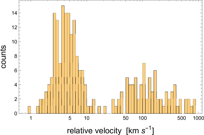
Figure 1: Histogram of estimated relative orbital velocity differences for 236 resolved double stars with independently determined Hipparcos and Gaia DR2 astrometric parameters.

Using the 2-norm option (i.e., nonlinear least-squares optimization) with weights constructed from the formal errors in Hipparcos and Gaia for each of the four condition equations, a unique set of parameters $\{E_{1},E_{2},e,n\}$ can be computed. These solutions are often of low value, however, due to the insufficient signal-to-noise ratios. To estimate the uncertainty of the results, extensive Monte Carlo simulations were performed for all 151 pairs using parallel computing in Mathematica. The observed data points $\boldsymbol{d}_{1}$ and $\boldsymbol{d}_{2}$ were additively perturbed by Gaussian-distributed random variables with a zero mean and standard deviations equal to their combined formal errors. For each trial, a set of 101 perturbed data vectors was generated, and a complete optimization solution obtained for each realization by the Random Search algorithm. The latter was found to perform somewhat better than the more traditional gradient or simulated annealing techniques because of multiple local minima of the merit function in the examined parameter space. The quantiles of the emerging distributions of eccentricity and orbital period $P_{\rm orb}=2\pi/n$ provide confidence intervals of the estimated two-point solutions.

Fig. 2 shows the distribution of eccentricity and $\log P$ values for one specific system HIP 10542 = WDS $02158-1814$. It is a known visual double with estimated $e=0.2$ and $P=330$ yr (Izmailov, 2019) extensively studied by speckle imaging (Horch et al., 2000; Mason et al., 2004; Horch et al., 2006; Tokovinin et al., 2010, 2015). Although the Monte Carlo trials do cluster around the known period at small eccentricity, the eccentricity itself is not well constrained, with clumps at $e=0$, $e=1$ and a separate group of bogus solutions with high $e$ and unreasonably long periods $\log P>3$. This illustrates a rather common issue with the two-point orbit estimation. Some combinations of randomly perturbed data yield runaway solutions with eccentricity values often piling up to the upper bound and unrealistically long periods. The majority of other stars show a similar pile-up at $e=0.99$, which was a hard constraint on the optimization. A poor condition of eccentricity is a known generic problem for astrometric orbital evaluation, which was encountered, for example, in Hipparcos-only estimation of short-period binaries (Goldin & Makarov, 2006).

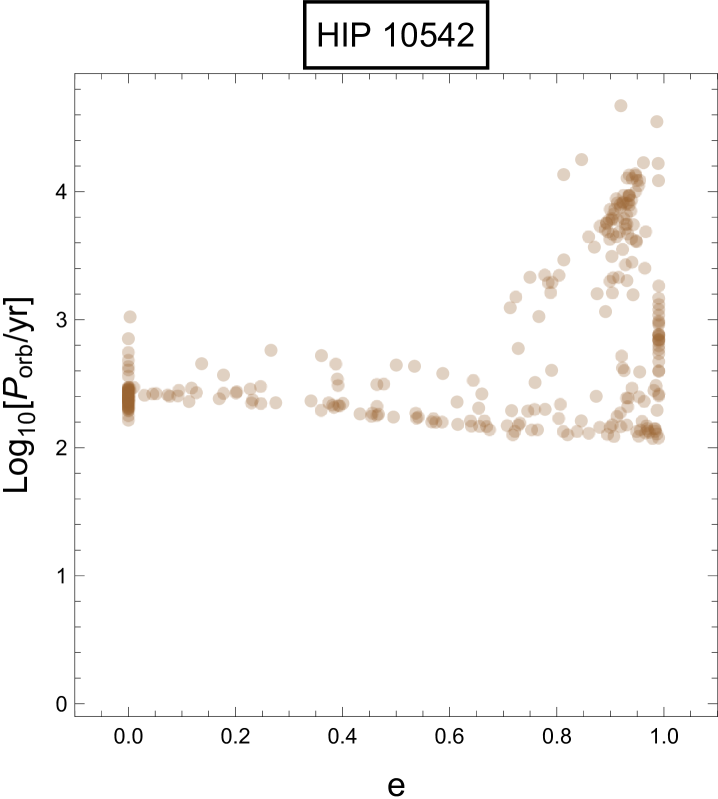
Figure 2: Results of 301 Monte-Carlo simulations of two-point orbit solutions for the physical binary HIP 10542 resolved in Hipparcos and Gaia DR2.

5 Possible improvements and experiments with artificial data

The basic algorithm of two-point orbit estimation described above seeks a solution for four orbital parameters $\{E_{1},E_{2},e,n\}$ after explicit elimination of the Thiele-Innes coefficients using the Gaia data point. However, this set of unknowns is redundant, because there are only 7 independent orbital elements. One can eliminate this redundancy by introducing one additional constraint from the Kepler’s equation:

$$e\,(\sin E_{2}-\sin E_{1})=E_{2}-E_{1}-n\,\Delta t,$$ (10)

where $\Delta t$ is the epoch difference, which equals to 24.25 years for the Hipparcos and Gaia DR2 data sets. Technically, this can be implemented as a constrained nonlinear optimization problem, making the solution somewhat more computer-intensive. At first glance, this should improve the performance, because the number of degrees of freedom is reduced by one. In reality, as my numerical experiments with artificial noiseless data revealed, it only helps to achieve a more accurate solution in the case of negligibly small noise. No significant improvement has been found when applied to the real data in hand. As a possible explanation, we note that statistical flukes or large errors in combination with the additional hard constraint linking the eccentric anomalies (Eq. 10) can perturb the parameters of significance $e$ and $n$ even more.

Another possible improvement concerns the possibility of more stable solutions on a grid of eccentric anomalies at first epoch, $E_{1}$. Fixing this less essential parameter, rather than orbital eccentricity, may provide insight into the overall behavior and condition of the optimization process, as well as help to identify the global minimum of the merit function. To test this hypothesis, I generated synthetic relative positions and proper motions at the relevant epochs 1991.25 and 2015.5 for a binary systems with $i=75\arcdeg$, $\omega=120\arcdeg$, $\Omega=200\arcdeg$, $T_{0}=1900$, $P_{\rm orb}=500$ yr, $e=0.4$, $M_{\rm tot}=2M_{\sun}$ at 100 pc from the Sun. The simulated data sets were processed with the constrained method using different nonlinear optimization techniques: random seeded search, Nelder-Mead, differential evolution, and simulated annealing. The random search solution with 400 search points produced a very good result, with $e=0.387$, $n=0.011$ rad$/$yr. The other algorithms fail to converge to the true orbit, leaving significant errors in $e$ and $n$ despite the anomaly condition Eq. 10 being rigorously satisfied. The reason for this is the complex structure of the merit function within the allowed multi-dimensional parameter space taking numerous minima, which may only be slightly larger than the true (global) minimum.

Mapping the entire parameter space is not feasible, but further insight can be gained by fixing $E_{1}$, which is more restrictive than fixing $e$. The random search and Nelder-Mead methods produce practically perfect solutions if $E_{1}$ value is fixed at the true value (1.5466 rad). Searching for the global minimum may then be implemented on a sufficiently dense grid of fixed $E_{1}$. Using the Nelder-Mead algorithm, which is much faster, I produced orbit solutions for a grid of 360 values $E_{1}=0,1,2,\ldots,359\arcdeg$. Fig. 3 shows the values of the merit function $||\mathbf{S}\cdot\boldsymbol{d_{1}}-\boldsymbol{d_{2}}||$ (left) and the fitted eccentricity $e$ (right) for this grid. Unfortunately, there is a plateau of $E_{1}$ values where the merit function is close to 0, which implies that this optimization is intrinsically uncertain (ill-conditioned). The corresponding estimates of $e$ group around the true value $0.4$, but with some obvious scatter.

Figure 3: Results of 360 two-point orbit solutions for a synthetic binary system with a period of 500 yr and noiseless data. The first-epoch eccentric anomaly was fixed on a grid of values covering the interval 0 to $2\pi$.

6 Estimating orbital periods at fixed eccentricity and comparison with Izmailov 2019 catalog

In view of the poor condition of two-epoch solutions for eccentricity, a more modest objective was set to derive estimates of orbital periods for 151 binary star systems at three fixed eccentricities: $e=0$, 0.5, and 0.9. The other three unknowns entering the epoch transformation matrix (Eq. 8) were constrained in the random search optimization: $E_{1}\in[0,2\pi]$, $E_{2}\in[0,2\pi]$, $n\in[n_{\rm est}/20$, $n_{\rm est}\cdot 10]$, where $n_{\rm est}=\sqrt{0.5\;(\rho/\varpi)^{3}}$, and both the separation $\rho$ and parallax $\varpi$ were extracted from the Gaia data. The hard condition on eccentric anomalies was not used in this experiment. The benchmark $n_{\rm est}$ is a crude estimate of the mean motion. The actual mean motion may deviate for various reasons, including the total mass being different from the assumed $2\,M_{\sun}$, the semimajor axis being likely greater than the observed separation due to the projection effect, the semimajor axis sometimes being smaller than the observed separation due to an eccentric orbit observed closer to the apoastron. The bounds on $n$ are meant to limit runaway solutions and provide a clear indication of failed optimizations.

The sample median period of $e=0$ solutions is $\sim 630$ yr. In each eccentricity sample, 20 to 23 solutions bump into the upper constraint $20\,P_{\rm est}$ resulting in a $>14$% rate of runaway solutions. A much higher rate of failed solution emerges from a comparison with the catalog of orbital parameters by Izmailov (2019). I found 83 systems in common with this catalog, 5 of which are known triple systems where two-point estimates cannot be valid. Only 14 solutions qualify as “good quality”, whereas 43 systems are a total mismatch. The latter often have unreasonably long periods in excess of 2000 years. It appears that the method tends to fit the observed position and velocity differences as a high-eccentricity orbital motion close to the periastron of otherwise a slow orbit.

Fixed-$E_{1}$ grid solutions applied in §5 to synthetic data can be used to gain some understanding of the failed fits. Fig. 4 shows the Nelder-Mead solutions for one of the unsuccessful cases, the binary system HIP 69442. According to Izmailov (2019), the expected orbital period is 1355 years and the eccentricity is 0.81. Although the merit function (left plot) has a well-defined minimum at around $E_{1}=4$, the corresponding eccentricity estimates (right plot) do not show any clumping, with many fits bumping into the upper or lower constraints. The period estimates are all bound to the upper limit. The four condition equations (7) in this case are weighted with weights inversely proportional to the combined formal errors of the corresponding data from Hipparcos and Gaia. Nominally, the squared norm of the residual vector is expected to be equal to the mean of $\chi^{2}_{4}$, which is 4. We can see that in this case the range of merit function values is quite narrow, with the smallest values much greater than the expected value. This implies that the fitting model is inconsistent with the present data. To summarize, a failed solution can be spotted by 1) lack of consistent eccentricity estimates around the global minimum; 2) best solutions bumping into the hard constraints on eccentricity or period; 3) smallest merit function values being too large compared to the expectation.

Figure 4: Results of 360 two-point orbit solutions for HIP 69442 on a grid of fixed first-epoch eccentric anomaly $E_{1}$, obtained with the Nelder-Mead optimization method. This data set also produced inconsistent solutions with the fixed-eccentricity option.

7 Summary and discussion

The technique of two-epoch orbit evaluation is viable in principle, but the practical difficulties arising in working with real space astrometry data indicate some deficiencies. I believe the main problems are the relatively modest precision of Hipparcos data for resolved double stars, especially the proper motions, and the intrinsic poor condition of the full-rank optimization problems. Hipparcos could confidently measure only stars brighter than magnitude $\sim 9$, but the situation was further exacerbated by the blending of signal from the components at separations up to 20 arcsec. As a result, the magnitude difference had to be small for a reliable determination of the secondary’s proper motion to be made. The output of the Hipparcos data reduction process was sensitive to initial assumptions about the components. Incorrect initial assumptions sometimes led to gross errors even for apparently single stars (Fabricius & Makarov, 2000). It is not known if the formal errors of astrometry are realistic for DMSA, so that our selection of S$/$N $>3$ cases does not let statistical flukes through.

On the other hand, Gaia has a vastly better dynamical range and better resolved tracking patches. Millions of resolved double stars are present in DR2 with individual proper motions, despite the absence of a dedicated double star pipeline. Being overall of much better quality, the Gaia part of the input data may still be subject to physical perturbations and errors. Hierarchical multiple systems are common, and the proper motion of unresolved tight pairs is perturbed by astrometric binarity (Wielen et al., 1999; Makarov & Kaplan, 2005). For Gaia, even large planets around nearby stars can be detectable from proper motion perturbations (Kaplan & Makarov, 2003). Such complicated cases require models with larger numbers of unknowns, for which the two-epoch technique provides bogus results. Finally, a fraction of the Hipparcos-Gaia sample may be optical doubles. The proper motion differences in this case reflect only the chance relative motion of two independent stars and random errors in the two catalogs.

It is more difficult to tackle the intrinsic poor condition of the two-epoch orbit solution, but there may be possible ways to improve this as well. The method is expandable with more position measurements. For example, if reliable angular separation and position angle measurements are available from, e.g., ground-based speckle interferometry or long-baseline optical interferometry, they can be incorporated into the main matrix equation 7 by adding two lines in matrix $\bf{S}$ with one additional unknown $E_{3}$, two new data points, and one additional hard constraint on $E_{3}$ from the Kepler’s equation. The method then becomes a three-epoch estimation. Furthermore, spectroscopic radial velocity measurements of both companions can be utilized as well, either as additional conditions in the matrix equation, or simply as additional constraints in the optimization procedure.

Finally, the future plans for astrometric space missions open up excellent prospects for the proposed method. The current Gaia mission could be used as the first epoch for millions of visual double stars, while a Gaia-NIR successor (Hobbs et al., 2019; McArthur et al., 2019) would provide the second point separated by 20–25 years in time with an equal or higher accuracy. The current techniques of ground-based orbit determination (speckle imaging, long-baseline optical interferometry) will prove insufficient to process that great a number of targets. As we move to distances beyond $\sim 100$ pc, angular separations become smaller, proper motion differences caused by orbital motion become smaller too. The sample of characterized wide binaries can be greatly enlarged by an ultra-precise astrometric instrument, such as the anticipated performance of the narrow-angle, differential astrometry mission Theia (The Theia Collaboration et al., 2017).

Appendix

A compilation of 1295 resolved double star pairs with individual component measurements in Hipparcos and Gaia DR2 (i.e., components’ positions, parallaxes, and proper motions) is published as an online-only table. It includes 2590 rows divided into 1295 pairs. Each pair of rows include data for the A component (nominally, the brighter one in Hipparcos) in the first row followed by a row of B component data. Each row contains 26 data fields. The contents of this table are described in Table 1.

Table 1: Resolved double star pairs with individual component measurements in Hipparcos and Gaia DR2

Number	Units	Description
1	—	Hipparcos identification number
2	mag	$H_{p}$ magnitude
3	deg	Hipparcos right ascension in degrees
4	deg	Hipparcos declination in degrees
5	mas	Hipparcos parallax
6	mas yr-1	Hipparcos proper motion in right ascension times $\cos\delta$
7	mas yr-1	Hipparcos proper motion in declination
8	mas	formal error of Hipparcos right ascension times $\cos\delta$
9	mas	formal error of Hipparcos declination
10	mas	formal error of Hipparcos parallax
11	mas yr-1	formal error of Hipparcos proper motion in right ascension times $\cos\delta$
12	mas yr-1	formal error of Hipparcos proper motion in declination
13	—	Gaia source id
14	deg	Gaia right ascension in degrees
15	deg	Gaia declination in degrees
16	mas	Gaia parallax
17	mas yr-1	Gaia proper motion in right ascension times $\cos\delta$
18	mas yr-1	Gaia proper motion in declination
19	mas	formal error of Gaia right ascension times $\cos\delta$
20	mas	formal error of Gaia declination
21	mas	formal error of Gaia parallax
22	mas yr-1	formal error of Gaia proper motion in right ascension times $\cos\delta$
23	mas yr-1	formal error of Gaia proper motion in declination
24	mag	Gaia $G$ magnitude
25	mag	Gaia $B_{p}$ magnitude
26	mag	Gaia $R_{p}$ magnitude

Note. — Table 1 is published in its entirety in the electronic edition of the Astronomical Journal. A portion is shown here for guidance regarding its form and content. Hipparcos astrometric data refer to the mean epoch of $1991.25$. Gaia DR2 data refer to the mean epoch of $2015.5$.

References

- Arenou et al. (2018) Arenou, F., Luri, X., Babusiaux, C., et al. 2018, A&A, 616, A17
- Brown & Gaia Collaboration (2018) Brown, A. G. A., Vallenari, A., Prusti, T., and Gaia Collaboration, 2018, A&A, 616, A1
- Descamps (2005) Descamps, P. 2005, Celestial Mechanics and Dynamical Astronomy, 92, 381
- ESA (1997) ESA, 1997, The Hipparcos Catalogue, ESA SP-1200, Vol. 1-17
- Fabricius & Makarov (2000) Fabricius, C., & Makarov, V. V. 2000, A&AS, 144, 45
- Gaia Collaboration et al. (2016) Gaia Collaboration, Prusti, T., de Bruijne, J. H. J., et al. 2016, A&A, 595, A1
- Goldin & Makarov (2006) Goldin, A., & Makarov, V. V. 2006, ApJS, 166, 341
- Heintz (1978) Heintz, W.D., 1978, Double Stars, D. Reidel Publishing Company
- Hobbs et al. (2019) Hobbs, D., Brown, A., Høg, E., et al. 2019, arXiv e-prints, arXiv:1907.12535
- Horch et al. (2000) Horch, E., Franz, O. G., & Ninkov, Z. 2000, AJ, 120, 2638
- Horch et al. (2006) Horch, E. P., Baptista, B. J., Veillette, D. R., et al. 2006, AJ, 131, 3008
- Izmailov (2019) Izmailov, I. S. 2019, Astronomy Letters, 45, 30
- Kaplan & Makarov (2003) Kaplan, G. H., & Makarov, V. V. 2003, Astronomische Nachrichten, 324, 419
- Kervella et al. (2019) Kervella, P., Arenou, F., Mignard, F., et al. 2019, A&A, 623, A72
- Lindegren et al. (1997) Lindegren, L., Mignard, F., Söderhjelm, S., et al. 1997, A&A, 323, L53
- Makarov & Unwin (2015) Makarov, V. V., & Unwin, S. C. 2015, MNRAS, 446, 2055
- Makarov & Kaplan (2005) Makarov, V. V., & Kaplan, G. H. 2005, AJ, 129, 2420
- Mason et al. (2004) Mason, B. D., Hartkopf, W. I., Wycoff, G. L., et al. 2004, AJ, 128, 3012
- McArthur et al. (2019) McArthur, B., Hobbs, D., Høg, E., et al. 2019, BAAS, 51, 118
- Ochsenbein et al. (2000) Ochsenbein, F., Bauer, P., & Marcout, J. 2000, A&AS, 143, 23
- Perryman (2009) Perryman, M. 2009, Astronomical Applications of Astrometry, Cambridge University Press, Cambridge UK
- Söderhjelm (1999) Söderhjelm, S. 1999, A&A, 341, 121
- The Theia Collaboration et al. (2017) The Theia Collaboration, Boehm, C., Krone-Martins, A., et al. 2017, arXiv e-prints, arXiv:1707.01348
- Tokovinin et al. (2010) Tokovinin, A., Mason, B. D., & Hartkopf, W. I. 2010, AJ, 139, 743
- Tokovinin (2014) Tokovinin, A. 2014, AJ, 147, 87
- Tokovinin et al. (2015) Tokovinin, A., Mason, B. D., Hartkopf, W. I., et al. 2015, AJ, 150, 50
- Tokovinin & Kiyaeva (2016) Tokovinin, A., & Kiyaeva, O. 2016, MNRAS, 456, 2070
- Wielen et al. (1999) Wielen, R., Dettbarn, C., Jahreiß, H., et al. 1999, A&A, 346, 675