Mean first-passage time to a small absorbing target in an elongated planar domain

Abstract

We derive an approximate but fully explicit formula for the mean first-passage time (MFPT) to a small absorbing target of arbitrary shape in a general elongated domain in the plane. Our approximation combines conformal mapping, boundary homogenisation, and Fick-Jacobs equation to express the MFPT in terms of diffusivity and geometric parameters. A systematic comparison with a numerical solution of the original problem validates its accuracy when the starting point is not too close to the target. This is a practical tool for a rapid estimation of the MFPT for various applications in chemical physics and biology.

I Introduction

The concept of first-passage time (FPT) is ubiquitous in describing phenomena around us. Being originally stemmed from the theory of Brownian motion as a time taken for a diffusing particle to arrive at a given location, nowadays it is widely used in chemistry (geometry-controlled kinetics), biology (gene transcription, foraging behaviour of animals) and many applications (financial modelling, forecasting of extreme events in the environment, time to failure of complex devices and machinery, military operations). This subject has an extensive literature, see Redner_2001 ; Bray_2013 ; Metzler_2014 ; Benichou_2014 ; Bressloff_2015 ; Holcman_2015 ; Lindenberg_2019 ; Dagdug_2015 ; Oshanin_2009 ; Lindsay_2017 ; Grebenkov_2016 ; Skvortsov_2018 ; Skvortsov_2020 ; Grebenkov_2020 ; Grebenkov_2019 and references therein. There is also a rich variety of different physical phenomena that can be analytically treated with the framework of the FPT due to similarity of underlying equations Bazant_2016 .

In a basic setting, the first-passage problem is formulated in the following way. We consider a Brownian particle initially located at point r of a bounded domain $\Omega$ and searching for a small target $\mathcal{S}$ (a small region with absorbing boundary) inside that domain (if the target is at the boundary the problem is usually referred to as the narrow escape problem Holcman_2015 ). As the first-passage time of the particle to the target is a random variable, its full characterisation requires the computation of its distribution Mejia12 ; Rupprecht15 ; Godec_2016a ; Godec_2016b ; Lanoiselee_2018 ; Grebenkov_2018a ; Grebenkov_2018b ; Grebenkov_2019b . In many practical situations, however, it is enough to estimate the average time $T(\textbf{r})$ taken for the particle to hit the target (see Redner_2001 ; Metzler_2014 ; Benichou_2014 ; Condamin_2007 ; Benichou_2008 ; Benichou_2010 ; Guerin_2016 and references therein). The mean first-passage time (MFPT) satisfies the Poisson equation Redner_2001

$$D\Delta T(\textbf{r})=-1,$$ (1)

where $D$ is the particle diffusivity, and $\Delta$ is the Laplace operator. The boundary of the domain is assumed reflecting, ${\partial T}/{\partial n}=0$ on $\textbf{r}\in\partial\Omega$ (with $\partial/\partial n$ being the normal derivative) and the target surface is absorbing, $T=0$ on $\textbf{r}\in\partial\mathcal{S}$.

In spite of an apparent simplicity of Eq. (1) and a variety of powerful methods for its analysis, to date the exact closed-form solutions of Eq. (1) are available only for a few special cases and for the domains with high symmetry such as a sphere or a disk Redner_2001 . Many approximate solutions, derived by advanced asymptotic methods, can produce a remarkable agreement with numerical solutions of Eq. (1), but often require specific mathematical expertise and still involve some level of numerical treatment Metzler_2014 ; Benichou_2014 ; Holcman_2015 ; Lindsay_2017 ; Grebenkov_2016 ; Singer06a ; Singer06b ; Singer06c ; Pillay10 ; Cheviakov10 ; Cheviakov12 ; Caginalp12 ; Marshall16 ; Ward_2020 . This necessitates the development of analytical approximations that being perhaps less accurate can lead to simple explicit expressions that provide reasonable estimations for MFPT in some general geometric settings. This was one of the main motivations for the present study.

The aim of the paper is to derive a general formula for the MFPT in an elongated planar domain with reflecting boundaries. The profile of the domain is assumed to be smooth, slowly changing, but otherwise general. The target is assumed to be small but of an arbitrary shape. We validate our findings by numerical solution of Eq. (1) via a finite elements method. Remarkably, this simple general formula, derived under a number of simplified approximations, turns out to be surprisingly accurate.

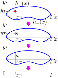
Figure 1: Three-step transformation of the original MFPT problem into an effectively one-dimensional problem with semi-permeable semi-absorbing boundary condition.

II Approximation for the MFPT

We consider an elongated planar domain of “length” $l$, which is determined by two smooth profiles $h_{-}(x)<h_{+}(x)$ (Fig. 1):

$$\Omega=\{(x,y)\in{\mathbb{R}}^{2}~{}:~{}0<x<l,~{}h_{-}(x)<y<h_{+}(x)\}.$$ (2)

In particular, the local “width” of the domain is $h(x)=h_{+}(x)-h_{-}(x)$, and $h_{0}=\max\{h(x)\}$ is the maximal width. Throughout the paper, we assume that the aspect ratio $h_{0}/l$ of the domain is small. A small absorbing target (also called trap or sink) is located inside the domain at some $(x_{T},y_{T})$, which is not too close to the boundary.

The main analytical formula will be derived by employing a three-step approximation. First, we replace the absorbing target by a vertical absorbing interval of the same trapping rate or the same conformal radius or the same logarithmic capacity (since they all are proportional to each other Landkof_1978 ). Far away from the target such a replacement is justifiable since at the distance greater than the size of the target (but still much smaller than $h(x_{T})$ and $l$) the absorption flux can be characterised by the first (monopole) moment of the shape of the target, and this equivalence preserves it. For a variety of planar shapes (circle, ellipse, arc, triangle, square, or even some fractals Ransford_2007 ; Ransford_2010 ), conformal radius is well-known or can be accurately estimated from various approximations, see Skvortsov_2018 ; Landkof_1978 ; Ransford_2010 and references therein. For instance, for an elliptical target with semi-axes $a$ and $b$, its conformal radius is $(a+b)/2$, so for an absorbing interval of length $s$ conformal radius is simply $s/4$ and this allows us to deduce the length of the equivalent absorbing interval $s$ for any given target.

Second, we substitute the absorbing interval at $x=x_{T}$ by an equivalent semi-permeable semi-absorbing vertical boundary. In line with the conventional arguments of effective medium theory, the trapping effect of the target can approximately be captured by means of this boundary with an effective reactivity $\kappa$. More specifically, we assume that the trapping rate of this effective boundary is equal to the trapping flux of the particles induced by the presence of the target. The well-known examples of such an approach are acoustic impedance of perforated screens Crocker_1998 and effective electric conductance of lattices and grids Tretyakov_2003 ; Hewett_2016 ; Marigo_2016 . The effective reactivity can be related to the geometrical parameters by employing the ideas of boundary homogenisation Skvortsov_2020 ; Hewett_2016 ; Marigo_2016 . In particular, an explicit form of this reactivity in the case of two absorbing arcs on the reflecting boundary of a disk of radius $R$ was found in Skvortsov_2020 . As shown in Skvortsov_2020 , an appropriate conformal mapping allows one to transform such a disk into an infinite horizontal stripe of width $2h$ with reflecting boundary that includes two identical absorbing intervals. By symmetry, this domain is also equivalent to a twice narrower stripe (i.e., of width $h$) with a single absorbing interval with a prescribed offset with respect to the reflecting boundary. Upon these transformations, the original formula of the effective reactivity is preserved, except that the perimeter of the disk, $2\pi R$, is replaced by the stripe width:

$$\kappa=\frac{D}{h(x_{T})}\frac{\pi}{\ln{(1/F)}}\,,$$ (3)

where

$$F=\sqrt{\sin^{2}[\tfrac{\pi}{2}(\sigma+\sigma_{g})]-\sin^{2}(\tfrac{\pi}{2}\sigma_{g})}\,,$$ (4)

with $\sigma=s/h(x_{T})$ and $\sigma_{g}=(y_{T}-s/2)/h(x_{T})$. Here, we used the width of the domain, $h(x_{T})$, at the location of the target. Even though Eq. (3) was derived for an infinite stripe, it is also applicable for an elongated rectangle of width $h(x_{T})$. Moreover, we will use it as a first approximation for general elongated domains.

Third, the Brownian particle, which is released at some point $(x,y)$ inside an elongated domain, frequently bounces from the horizontal reflecting walls while gradually diffusing along the domain towards the target. The shape of the horizontal walls (defined by $h_{\pm}(x)$) can additionally create an entropic drift, which can either speed up or slow down the arrival to the target. In any case, the information about the particle initial location in the vertical direction, $y$, becomes rapidly irrelevant, and the original MFPT problem, Eq. (1), is reduced to a one-dimensional problem. While the classical Fick-Jacobs equation determines the concentration $c(x,t)$ averaged over the cross-section (see Zwanzig_1992 ; Reguera_2001 ; Kalinay_2006 ; Bradley_2009 ; Rubi_2010 ; Dagdug_2012 and references therein), the survival probability is determined by the backward diffusion equation with the adjoint diffusion operator Gardiner . In particular, Eq.(1) in an elongated domain reduces to

$$\frac{D}{h(x)}\frac{d}{dx}\biggl{[}h(x)\frac{dT(x)}{dx}\biggr{]}=-1\,.$$ (5)

In summary, we transformed the original problem of finding the MFPT to a small target of arbitrary shape in a general elongated domain to the one-dimensional problem, which can be solved analytically.

Domain	$y(z)$	$Y(z)$	$U_{-}(z)$	$U_{+}(z)$	$Y(1)$	$C_{y}$
Rectangular	$1$	$z$	$\tfrac{1}{2}z^{2}$	$U_{-}(1-z)$	$1$	$\tfrac{1}{6}$
Triangular	$z$	$\tfrac{1}{2}z^{2}$	$\tfrac{1}{4}z^{2}$	$\tfrac{1}{4}(z^{2}-1-2\ln z)$	$\tfrac{1}{2}$	$\tfrac{1}{8}$
Rhombic	$1-|2z-1|$	$\left\{\begin{array}[]{ll}z^{2}&(z<\tfrac{1}{2})\\ \tfrac{1}{2}-(1-z)^{2}&(z>\tfrac{1}{2})\\ \end{array}\right.$	$\left\{\begin{array}[]{ll}\tfrac{1}{4}z^{2}&(z<\tfrac{1}{2})\\ \frac{(1-z)^{2}-\ln(2-2z)}{4}&(z>\tfrac{1}{2})\\ \end{array}\right.$	$U_{-}(1-z)$	$\tfrac{1}{2}$	$\tfrac{3}{32}$
Sinusoidal	$\sin(\pi z)$	$\frac{1}{\pi}(1-\cos(\pi z))$	$\frac{1}{\pi^{2}}\bigl{(}\ln 2-\ln(1+\cos(\pi z))\bigr{)}$	$U_{-}(1-z)$	$\tfrac{2}{\pi}$	$\tfrac{1}{\pi^{2}}$
Parabolic	$4z(1-z)$	$2z^{2}(1-2z/3)$	$\tfrac{1}{6}\bigl{(}z^{2}-z-\ln(1-z)\bigr{)}$	$U_{-}(1-z)$	$\tfrac{2}{3}$	$\tfrac{19}{180}$
Elliptic	$\sqrt{1-(2z-1)^{2}}$	$\begin{array}[]{l}\tfrac{\pi}{8}+\tfrac{1}{4}\mathrm{asin}(2z-1)\\ -(\tfrac{1}{2}-z)\sqrt{z(1-z)}\\ \end{array}$	$\begin{array}[]{l}\frac{\pi^{2}}{64}+\frac{z(z-1)}{4}+\frac{\mathrm{asin}^{2}(2z-1)}{16}\\ +\frac{\pi}{16}\mathrm{asin}(2z-1)\end{array}$	$U_{-}(1-z)$	$\tfrac{\pi}{4}$	$\frac{\pi^{2}}{48}-\tfrac{5}{64}$

Table 1: Several examples of symmetric elongated domains defined by setting $-h_{-}(x)=h_{+}(x)=\tfrac{1}{2}h(x)=\tfrac{1}{2}\,h_{0}\,y(x/l)$: the rescaled profile $y(z)$, its integral $Y(z)$, functions $U_{\pm}(z)$ from Eq. (10), the rescaled area $Y(1)$ (such that $S=lh_{0}Y(1)$), and the shape-dependent constant $C_{y}$ from Eq. (15). For all domains, which are symmetric with respect to the vertical line at $l/2$, one has $U_{+}(z)=U_{-}(1-z)$.

We search for the solution of Eq. (5) in the intervals $(0,x_{T})$ and $(x_{T},l)$. Multiplying this equation by $h(x)/D$, integrating over $x$ and imposing Neumann (reflecting) boundary conditions at $x=0$ and $x=l$, we get

$$T(x)=\left\{\begin{array}[]{l l}\displaystyle C_{-}-\int\nolimits_{0}^{x}dx^{\prime}\frac{S(x^{\prime})}{Dh(x^{\prime})}&(0<x<x_{T}),\\ \displaystyle C_{+}-\int\nolimits_{x}^{l}dx^{\prime}\frac{S(l)-S(x^{\prime})}{Dh(x^{\prime})}&(x_{T}<x<l),\\ \end{array}\right.$$ (6)

where $S(x)=\int\nolimits_{0}^{x}dx^{\prime}\,h(x^{\prime})$ is the area of (sub)domain restricted between $0$ and $x$. The integration constants $C_{\pm}$ are determined by imposing the effective semi-permeable semi-absorbing boundary condition at the target location:

$$T(x_{T}-0) =T(x_{T}+0),$$ (7a)

$$D\left[\frac{dT}{dx}(x_{T}+0)-\frac{dT}{dx}(x_{T}-0)\right] =\kappa\,T(x_{T}).$$ (7b)

The first relation ensures the continuity of the MFPT, whereas the second condition states that the difference of the diffusive fluxes at two sides of the semi-permeable boundary at $x_{T}$ is equal to the reaction flux on the target. The latter flux is proportional to $T(x_{T})$, with an effective reactivity $\kappa$ from Eq. (3).

Substituting Eq. (6) into Eqs. (7), we get the final solution of the problem:

$$T(x)=\frac{l^{2}}{D}\biggl{(}U_{\sigma_{x}}(x_{T}/l)-U_{\sigma_{x}}(x/l)\biggr{)}+\frac{l}{\kappa}\,\frac{Y(1)}{y(x_{T}/l)}\,,$$ (8)

where $y(z)$ is the rescaled profile, $h(x)=h_{0}y(x/l)$ (with $z=x/l$), and

$$Y(z) =\int\limits_{0}^{z}dz^{\prime}\,y(z^{\prime}),$$ (9)

$$U_{-}(z) =\int\limits_{0}^{z}dz^{\prime}\,\frac{Y(z^{\prime})}{y(z^{\prime})},\quad U_{+}(z)=\int\limits_{z}^{1}dz^{\prime}\,\frac{Y(1)-Y(z^{\prime})}{y(z^{\prime})}\,.$$ (10)

The subscript $\sigma_{x}$ in Eq (8) depends on $x$ as being determined by the sign of difference $x-x_{T}$: $\sigma_{x}=+$ for $x>x_{T}$ and $\sigma_{x}=-$ for $x<x_{T}$. The functions $Y(z)$ and $U_{\pm}(z)$ in Eq. (8) can be easily computed for a given profile $h(x)$ (or $y(z)$) either analytically (see Table 1) or numerically. For instance, in the simplest case of the rectangular domain, $h_{\pm}(x)=\pm h_{0}/2$, we get

$$T(x)=\left\{\begin{array}[]{l l}\displaystyle\frac{x_{T}^{2}-x^{2}}{2D}+\frac{l}{\kappa}&~{}~{}(0\leq x\leq x_{T}),\\ \displaystyle\frac{(x-x_{T})(2l-x_{T}-x)}{2D}+\frac{l}{\kappa}&~{}~{}(x_{T}\leq x\leq l),\\ \end{array}\right.$$ (11)

Other examples are summarised in Table 1 and presented below.

The explicit Eq. (8) constitutes the main result of the paper and includes two terms. The first (diffusion) term is independent of the size of the target and is related to the time required for a Brownian particle to arrive at the proximity to the target from its starting position. For this reason, the contribution of this term is small when $x\approx x_{T}$, i.e. when the particle initial position is near the target. The second (reaction) term in Eq. (11) describes the particle absorption by the target when the particle starts in its vicinity. This term diverges logarithmically as the target size decreases and thus dominates in the small target limit.

In many applications, the starting point is not fixed but uniformly distributed inside the domain. In this setting, one often resorts to the surface-averaged MFPT:

$$\overline{T}=\frac{1}{S}\int\limits_{\Omega}dxdy\,T(x,y).$$ (12)

Substituting our approximate solution (8), we get an explicit approximation for $\overline{T}$:

$$\overline{T}_{\rm app}=\frac{l^{2}}{D}\int\limits_{0}^{1}dz\,\frac{y(z)}{Y(1)}\bigl{(}U_{\sigma_{zl}}(z_{T})-U_{\sigma_{zl}}(zl)\bigr{)}+\frac{l}{\kappa}\frac{Y(1)}{y(z_{T})}\,,$$ (13)

where $z_{T}=x_{T}/l$. The last integral can be evaluated by using Eq. (10). After elementary but lengthy computations, we get

$$\overline{T}_{\rm app}=\frac{l^{2}}{D}\biggl{(}U_{-}(z_{T})+U_{+}(z_{T})-C_{y}\biggr{)}+\frac{l}{\kappa}\frac{Y(1)}{y(z_{T})}\,,$$ (14)

where

$$C_{y}=\int\limits_{0}^{1}dz\,\frac{Y(z)(Y(1)-Y(z))}{Y(1)y(z)}$$ (15)

is the shape-dependent constant.

III Conditions of validity

The main conditions that limit the range of validity of the proposed approximation come from the two underlying assumptions: (i) a relative smallness of the target with respect to all dimensions of the system ($s/h\ll 1$), and (ii) introduction of the effective trapping rate (along the domain) that can adequately characterise the target. The effective trapping rate will be formed at some distance from the target (since near the target it varies at much smaller scale $\sim s\ll h$) and this imposes some restriction on the elongation of the domain, as well as on the relative position of the starting point of the particle (e.g., the approximation may be inaccurate if the starting position is in the same cross-section as the target). In line with the previous studies Dagdug_2015 , this approximation is expected to provide reasonable estimations of the MFPT even when the target is not infinitesimally small and the longitudinal separation between the starting point of the particle and the target is of the order of the domain height.

A minor (geometrical) constraint is related to the proximity of the target to the reflecting boundary. If the distance between the target and the boundary is smaller than the half-length $s/2$ of the equivalent absorbing interval, the result will be indistinguishable from the scenario when the target is touching the boundary. Since we assume that the target is relatively small, $s/h\ll 1$, this limitation is insignificant.

More quantitative criteria for the validity of the proposed framework will be established below by numerical simulations.

IV Numerical Simulations

We validate our analytical approximation for the MFPT, Eq. (8), by comparison with the results of a direct numerical solution of the boundary value problem (1) by means of a Finite Element Method (FEM) solver implemented in Matlab PDEtool. First, we calculated MFPT in the rectangular domain for a circular target of radius $\rho$, so the length of the equivalent absorbing interval is $s=4\rho$. Figure 2(a) shows the MFPT, $T(x,y)$, for a circular target of radius $\rho=0.1$ located at $(1,-0.1)$ inside an elongated rectangle $\Omega=(0,5)\times(-\tfrac{1}{2},\tfrac{1}{2})$ with reflecting boundary (i.e., $l=5$ and $h_{0}=1$). In line with the above comments, our analytical approximation provides good estimates of the MFPT, except for the cases when the initial position of the particle is very close to the target (less than $h_{0}$). This condition provides a quantitative criterion for applicability of this analytical framework.

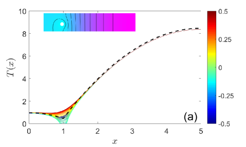
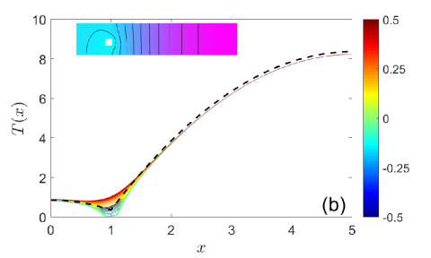
Figure 2: MFPT to a circular target of radius $\rho=0.1$ (a) and to a square target with edge length $a=0.2$ (b), which is located at $(1,-0.1)$ inside an elongated rectangle $(0,5)\times(-\tfrac{1}{2},\tfrac{1}{2})$ with reflecting boundary, with $D=1$. Comparison between our approximation Eq. (11) (shown by black dashed line) and the FEM solution (coloured lines) as a function of $x$ for 64 equally spaced $y$, from $y=-\tfrac{1}{2}$ (dark blue) to $y=\tfrac{1}{2}$ (dark red). Inset show the FEM solution $T(x,y)$ as coloured contour plots.

Next we analyse the effect of the target shape on the MFPT. To this end we consider the MFPT to a small absorbing square of side $a$ in the same rectangular domain, for which the length of the equivalent absorbing interval is $s=a\,\Gamma^{2}(1/4)/{\pi}^{3/2}\approx 2.36\,a$. Figure 2(b) shows a good agreement between our approximation and the FEM solution for a square of side $a=0.2$ at the same location inside the same rectangle as in Fig. 2(a). One can see that the target shape is correctly captured via its conformal radius.

To validate the proposed framework for other elongated domains we calculated the MFPT in three domains of different shape (an ellipse, a triangle, and a rhombus), for which we kept the same aspect ratio as before: $h_{0}/l=0.2$. A circular target of radius $\rho=0.1$ is located in different positions inside these domains. Figure 3 illustrates an excellent agreement between our approximation in Eq. (8) and numerical solutions for all these domains. We also checked that the relative error of the explicit approximation (14) for the surface-averaged MFPT, $\overline{T}$, does not exceed $2\%$ for all these examples (see Table 2).

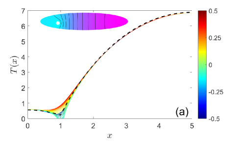
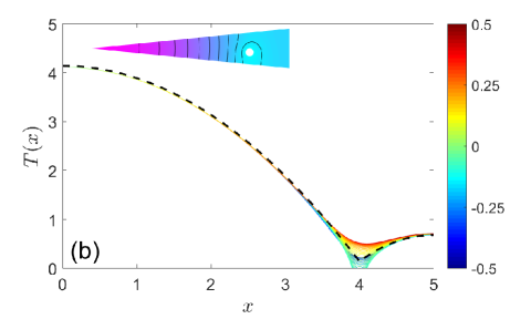
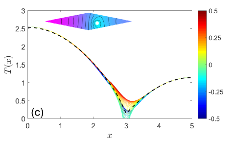
Figure 3: MFPT $T(x,y)$ to a circular target of radius $\rho=0.1$ inside an elongated domain with reflecting boundary, inserted into a rectangle $(0,5)\times(-\tfrac{1}{2},\tfrac{1}{2})$, with $D=1$ (obtained by FEM). (a) Ellipse, $(x_{T},y_{T})=(1,-0.1)$; (b) Triangle, $(x_{T},y_{T})=(4,-0.1)$; (c) Rhombus, $(x_{T},y_{T})=(3,-0.1)$. 64 coloured curves represent $T(x,y)$ as a function of $x$ for 64 equally spaced $y$, from $y=-\tfrac{1}{2}$ (dark blue) to $y=\tfrac{1}{2}$ (dark red). Black dashed line shows the approximate solution (8), with explicitly found functions $Y(z)$ and $U_{\pm}(z)$ in Table 1. Inset shows $T(x,y)$ inside each domain.

Domain	$\overline{T}$	$\overline{T}_{\rm app}$	relative error
Rectangular (circle)	4.7481	4.7961	$1\%$
Rectangular (square)	4.6128	4.6855	$2\%$
Triangular	1.5567	1.5522	$0.3\%$
Rhombic	1.2096	1.1888	$2\%$
Elliptic	4.0403	4.0340	$0.2\%$

Table 2: The surface-averaged MFPT, $\overline{T}$, estimated from the numerical solution of the original problem (solved by a FEM), and its explicit approximation $\overline{T}_{\rm app}$ from Eq. (14), for five examples shown in Figs. 2 and 3.

V Conclusion

We obtained a simple formula (8) for the MFPT to a small absorbing target of an arbitrary shape in an elongated planar domain with slowly changing boundary profile. This formula expresses MFPT in terms of dimensions of the domain, the form and size of the absorbing target and its relative position inside the domain. We validated our analytical predictions by numerical simulations and found excellent agreement. Indeed, if the initial position of the particle and the target location are well separated (more than half of the height of the domain at the target location $x_{T}$) then the numerical and analytical results are almost indistinguishable; but even for closer separations the analytical predictions are still reasonable, see Figs. 2 and 3. The proposed expression for the MFPT is a useful tool for some rapid practical estimations as well as for validation of complex numerical models of particle diffusion in geometrically constrained settings.

Future work may involve an extension of the proposed framework to more complex geometries (an elongated domain with an arbitrary piecewise boundary) or an extension to the three-dimensional settings. The main challenge in the three-dimensional case consists in finding an appropriate expression for the trapping rate of the target, i.e., a 3D generalisation of Eq. (3).

- (1) S. Redner, Guide to First Passage Processes (Cambridge University press, Cambridge, 2001)
- (2) A. J. Bray, S. Majumdar, and G. Schehr, Persistence and First-Passage Properties in Non-equilibrium Systems, Adv. Phys. 62, 225-361 (2013).
- (3) R. Metzler, G. Oshanin, and S. Redner (eds.) First-Passage Phenomena and Their Applications (World Scientific, Singapore, 2014).
- (4) O. Bénichou and R. Voituriez. From first-passage times of random walks in confinement to geometry-controlled kinetics. Phys. Rep. 539, 225-284 (2014).
- (5) P. Bressloff and S. D. Lawley. Stochastically gated diffusion-limited reactions for a small target in a bounded domain. Phys. Rev. E. 92, 062117 (2015).
- (6) K. Lindenberg, R. Metzler, and G. Oshanin (eds.) Chemical Kinetics: Beyond the Textbook (World Scientific, 2019).
- (7) G. Oshanin, O. Vasilyev, P. L. Krapivsky, and J. Klafter. Survival of an evasive prey, Proc. Nat. Acad. Sci. U.S.A. 106, 13696-13701 (2009)
- (8) A. E. Lindsay, A. J. Bernoff, and M. J. Ward. First passage statistics for the capture of a Brownian particle by a structured spherical target with multiple surface traps. SIAM J. Multi. Model. Simul. 15, 74-109 (2017).
- (9) D. Holcman and Z. Schuss, Stochastic Narrow Escape in Molecular and Cellular Biology (Springer, Berlin, 2015).
- (10) D. S. Grebenkov. Universal Formula for the Mean First Passage Time in Planar Domains, Phys. Rev. Lett. 117, 260201 (2016).
- (11) L. Dagdug, A. M. Berezhkovskii, and A. T. Skvortsov. Trapping of diffusing particles by striped cylindrical surfaces. Boundary homogenization approach. J. Chem. Phys. 142, 234902 (2015).
- (12) A. T. Skvortsov, A. M. Berezhkovskii, and L. Dagdug, Trapping of diffusing particles by spiky absorbers, J. Chem. Phys. 148, 084103 (2018).
- (13) A. T. Skvortsov. Mean first passage time for a particle diffusing on a disk with two absorbing traps at the boundary. Phys. Rev E 102, 012123 (2020).
- (14) D. S. Grebenkov, Paradigm shift in diffusion-mediated surface phenomena. Phys. Rev. Lett. 125, 078102 (2020).
- (15) D. S. Grebenkov. Imperfect diffusion-controlled reactions. In: K. Lindenberg, R. Metzler, and G. Oshanin (eds.) Chemical Kinetics: Beyond the Textbook, chap. 8, 191-219 (World Scientific, 2019).
- (16) M. Z. Bazant. Exact solutions and physical analogies for unidirectional flows, Phys. Rev. Fluids 1, 024001 (2016)
- (17) Mattos T, Mejía-Monasterio C, Metzler R, Oshanin G (2012) First passages in bounded domains: When is the mean first passage time meaningful? Phys. Rev. E 86:031143.
- (18) Rupprecht J-F, Bénichou O, Grebenkov DS, Voituriez R (2015) Exit time distribution in spherically symmetric two-dimensional domains. J. Stat. Phys. 158:192-230.
- (19) Godec A, Metzler R (2016) Universal proximity effect in target search kinetics in the few encounter limit. Phys. Rev. X 6:041037.
- (20) Godec A, Metzler R (2016) First passage time distribution in heterogeneity controlled kinetics: going beyond the mean first passage time. Sci. Rep. 6:20349.
- (21) Y. Lanoiselée, N. Moutal, and D. S. Grebenkov, Diffusion-limited reactions in dynamic heterogeneous media, Nature Commun. 9, 4398 (2018).
- (22) Grebenkov DS, Metzler R, Oshanin G (2018) Towards a full quantitative description of single-molecule reaction kinetics in biological cells. Phys. Chem. Chem. Phys. 20:16393-16401.
- (23) Grebenkov DS, Metzler R, Oshanin G (2018) Strong defocusing of molecular reaction times results from an interplay of geometry and reaction control. Commun. Chem. 1:96.
- (24) D. S. Grebenkov, R. Metzler, and G. Oshanin, Full distribution of first exit times in the narrow escape problem, New J. Phys. 21, 122001 (2019).
- (25) S. Condamin, O. Bénichou, V. Tejedor, R. Voituriez, and J. Klafter, First-passage time in complex scale-invariant media, Nature 450, 77-80 (2007).
- (26) Bénichou O, Voituriez R. Narrow-Escape Time Problem: Time Needed for a Particle to Exit a Confining Domain through a Small Window. Phys. Rev. Lett. 100, 168105 (2008).
- (27) O. Bénichou, C. Chevalier, J. Klafter, B. Meyer, and R. Voituriez, Geometry-controlled kinetics, Nature Chem. 2, 472-477 (2010).
- (28) T. Guérin, N. Levernier, O. Bénichou, and R. Voituriez, Mean first-passage times of non-Markovian random walkers in confinement, Nature 534, 356-359 (2016).
- (29) A. Singer, Z. Schuss, D. Holcman, and R. S. Eisenberg, “Narrow Escape, Part I”, J. Stat. Phys. 122, 437-463 (2006).
- (30) A. Singer, Z. Schuss, and D. Holcman, “Narrow Escape, Part II The circular disk”, J. Stat. Phys. 122, 465 (2006).
- (31) A. Singer, Z. Schuss, and D. Holcman, “Narrow Escape, Part III Riemann surfaces and non-smooth domains”, J. Stat. Phys. 122, 491 (2006).
- (32) S. Pillay, M. J. Ward, A. Peirce, and T. Kolokolnikov, “An Asymptotic Analysis of the Mean First Passage Time for Narrow Escape Problems: Part I: Two-Dimensional Domains”, SIAM Multi. Model. Simul. 8, 803-835 (2010).
- (33) A. F. Cheviakov, M. J. Ward, and R. Straube, “An Asymptotic Analysis of the Mean First Passage Time for Narrow Escape Problems: Part II: The Sphere”, SIAM Multi. Model. Simul. 8, 836-870 (2010).
- (34) A. F. Cheviakov, A. S. Reimer, and M. J. Ward, “Mathematical modeling and numerical computation of narrow escape problems”, Phys. Rev. E 85, 021131 (2012).
- (35) C. Caginalp and X. Chen, “Analytical and Numerical Results for an Escape Problem”, Arch. Rational. Mech. Anal. 203, 329-342 (2012).
- (36) J. S. Marshall, “Analytical Solutions for an Escape Problem in a Disc with an Arbitrary Distribution of Exit Holes Along Its Boundary”, J. Stat. Phys. 165, 920-952 (2016).
- (37) S. A. Iyaniwura, T. Wong, C. B. Macdonald, and M. J. Ward, Optimization of the Mean First Passage Time in Near-Disk and Elliptical Domains in 2-D with Small Absorbing Traps, Preprint in ArXiv 2006.12722 (2020).
- (38) N. Landkof. Foundations of Modern Potential Theory (Springer Verlag, Berlin, 1972).
- (39) T. Ransford and J. Rostand, Computation of capacity, Math. Comp. 76, 1499-1520 (2007).
- (40) T. Ransford, Computation of Logarithmic Capacity. Comput. Methods Func. Theory 10, 555-578 (2010).
- (41) M. J. Crocker, Handbook of Acoustics (John Wiley & Sons, Inc., New York, 1998)
- (42) S. Tretyakov. Analytical Modeling in Applied Electromagnetics (Artech House, UK 2003).
- (43) D. P. Hewett and I. J. Hewitt, Homogenized boundary conditions and resonance effects in Faraday cages, Proc. R. Soc. A 472, 20160062 (2016).
- (44) J. J. Marigo and A. Maurel, Two-scale homogenization to determine effective parameters of thin metallic-structured films, Proc. R. Soc. A 472, 20160068 (2016).
- (45) R. Zwanzig, Diffusion past an entropy barrier, J. Phys. Chem. 96, 3926-3930 (1992).
- (46) D. Reguera and J. M. Rubi, Kinetic equations for diffusion in the presence of entropic barriers. Phys. Rev. E 64, 061106 (2001).
- (47) P. Kalinay and J. K. Percus, Corrections to the Fick-Jacobs equation, Phys. Rev. E 74, 041203 (2006).
- (48) R. M. Bradley, Diffusion in a two-dimensional channel with curved midline and varying width: Reduction to an effective one-dimensional description, Phys. Rev. E 80, 061142 (2009).
- (49) J. M. Rubi and D. Reguera, Thermodynamics and stochastic dynamics of transport in confined media, Chem. Phys. 375, 518-522 (2010).
- (50) L. Dagdug, M. Vazquez, A. M. Berezhkovskii, V. Yu. Zitserman, and S. M. Bezrukov. Diffusion in the presence of cylindrical obstacles arranged in a square lattice analyzed with generalized Fick-Jacobs equation. J. Chem. Phys 136, 204106 (2012).
- (51) C. W. Gardiner, Handbook of stochastic methods for physics, chemistry and the natural sciences (Springer: Berlin, 1985).