Physics-constrained Bayesian inference of state functions in classical density-functional theory

Abstract

Abstract

We develop a novel data-driven approach to the inverse problem of classical statistical mechanics: given experimental data on the collective motion of a classical many-body system, how does one characterise the free energy landscape of that system? By combining non-parametric Bayesian inference with physically-motivated constraints, we develop an efficient learning algorithm which automates the construction of approximate free energy functionals. In contrast to optimisation-based machine learning approaches, which seek to minimise a cost function, the central idea of the proposed Bayesian inference is to propagate a set of prior assumptions through the model, derived from physical principles. The experimental data is used to probabilistically weigh the possible model predictions. This naturally leads to humanly interpretable algorithms with full uncertainty quantification of predictions. In our case, the output of the learning algorithm is a probability distribution over a family of free energy functionals, consistent with the observed particle data. We find that surprisingly small data samples contain sufficient information for inferring highly accurate analytic expressions of the underlying free energy functionals, making our algorithm highly data efficient. We consider excluded volume particle interactions, which are ubiquitous in nature, whilst being highly challenging for modelling in terms of free energy. To validate our approach we consider the paradigmatic case of one-dimensional fluid and develop inference algorithms for the canonical and grand-canonical statistical-mechanical ensembles. Extensions to higher-dimensional systems are conceptually straightforward, whilst standard coarse-graining techniques allow one to easily incorporate attractive interactions.

I Introduction

The past few years have seen an explosive development of machine learning (ML) methods, which enabled dramatic enhancements across such diverse fields as pattern recognition [1], natural language processing [2] and even DNA sequencing [3]. It is now generally accepted that adoption of ML methods has the potential to accelerate the development and enhance the quality of research across most scientific and engineering disciplines. Not surprisingly, we are witnessing the emergence of a number of fields at the intersection between ML and sciences-engineering: from quantum ML to data-centric engineering. Despite its advantages and numerous success stories, however, ML has yet to fulfil its full potential, especially in long-standing fundamental problems.

One such classical problem comes from the field of statistical mechanics, a branch of physics which aims to relate the observable macroscopic properties of matter with its underlying microscopic structure. Such properties as pressure, magnetisation or electric charge can all be determined by carefully averaging the small-scale interactions between the constituent particles of matter. The central property which facilitates such averaging is the one-body density function $\rho({\bf r})$, which can be thought of as the probability density function of finding a particle in the vicinity of the position-vector ${\bf r}$. Thus, a general method for obtaining $\rho({\bf r})$ of a given many-body system, poses a long-standing problem of fundamental importance to numerous scientific and engineering fields.

Even when the system particles interact via simple potentials, computing $\rho({\bf r})$ exactly is computationally intractable, due to inter-particle correlations. For example, application of the Liouville theorem leads to a hierarchy of density correlation functions and requires simplifying closure assumptions to make the resulting system of equations computable. A way out is offered by the density-functional theory (DFT), which is based on the mathematical fact that the free energy of a many-body system is a functional of its density $\rho({\bf r})$ and attains its minimum at the density of the system at equilibrium. In the subject literature the acronym DFT usually refers to one of the two generic classes of models: (i) quantum DFT, which deals with the exchange-correlation energy of quantised many-body systems, particularly electron gas [4, 5]; and (ii) classical DFT (cDFT), which applies to many-body systems with classical interactions such as common liquids, electrolytes, salts etc. and works with the Helmholtz free energy functional $F[\rho]$ [6, 7, 8].

The focus here is on the classical world. Ab initio quantum DFT calculations promise to realise the full potential of statistical mechanics. However, they are computationally forbidding for beyond-the-molecular-scale systems, despite drastic improvements in computational power. At the same time, classical statistical mechanics and cDFT are not totally disconnected from the quantum world as they subsume many quantum effects inside the particle interaction potentials. Not surprisingly, cDFT is a generic and widely used statistical mechanical framework for numerical and mathematical scrutiny.

Unfortunately, the payoff reaped by the DFT formulation of the many-body problem as the minimisation of the free energy is lessened by the fact that the exchange correlation energy in quantum DFT and the excess-over-ideal Helmholtz free energy in cDFT are not known exactly. This necessitates the development of methods to approximate these terms, which form the bulk of modern statistical-mechanical literature.

A popular intuitive and practical method for constructing DFT approximations is based on coarse-graining the intermolecular interactions [7]. Essentially, coarse-graining splits the unknown $F[\rho]$ of the system into appropriate reference and perturbation parts, treating them separately. The reference system describes the dominant interaction, which in many systems corresponds to the repulsive part of the full intermolecular potential. For example, interactions in a Lennard-Jones fluid consist of short-range repulsions, caused by the overlap of the electron orbitals and the Pauli exclusion principle, and comparatively weaker long-range attractions, caused by the dipole-dipole electromagnetic interaction. A coarse-grained approximate $F[\rho]$ is then given by the free energy of a hard sphere fluid with an added mean-field attractive term. Coarse-graining can be viewed as an extension of the Born-Oppenheimer approximation, whereby intermolecular effects occurring on different spatiotemporal scales are decoupled and accounted for separately.

The majority of realistic many-body systems can, in principle, be described by similar techniques. Indeed many studies have highlighted the potential utility of coarse-grained cDFTs in practical applications, including phase transitions, interfacial phenomena, colloidal and polymer fluids, surfactants, liquid crystals, crystalline solids, glasses and the rapidly growing fields of microfluidics [7, 9]. Yet, despite considerable efforts to bring cDFT to the applications domain [10, 11], existing cDFT approximations are mainly limited to highly idealised systems. Thus, present-day cDFT is still far from becoming an instrument of widespread practical utility and obtaining the status of a computational go-to framework, on a par with molecular dynamics (MD) and computational fluid dynamics [12].

As mentioned above, one important caveat is to adequately capture the reference system of purely repulsive hard particles of a given shape. In applications, fluid particles interact via complex potentials which makes the construction of DFTs in each case extremely difficult. There is a clear need for an algorithmic hands-off method for obtaining accurate and robust DFT functionals of purely repulsive systems. Coming to our rescue, modern statistical inference frameworks offer the principle means to develop just such a method.

While there is a growing number of ML works in quantum DFT, applications to classical many-body systems are still extremely rare. In Ref. 13, a Bayesian approach was developed to fit the drift of a Langevin equation, describing oscillations of an atom in a lattice. The posterior was sampled with sequential Monte-Carlo, which accommodates large datasets, but has the downside of being suitable only for parametric models with a small number parameters. The four parameters of a postulated ansatz for the inter-particle potential were fitted using simulation data. Unlike Ref. 13, where the number of parameters is fixed, our statistical model for $F[\rho]$ is non-parametric, thus possessing a high-level of flexibility. Our method is also technically more advanced in that it employs adjoint differentiation to evaluate the solution gradient on every step of the sampler. In Ref. 14, the choice of free energy terms is formulated as a classification problem employing a neural network (NN). The training is done by minimising the regularised Euclidean distance between the trained particle distribution and another distribution, obtained by averaging the simulation data. The choices of the NN architecture and the loss function are highly empirical. Additionally, raw simulation data requires costly post-processing, leading to information loss and compromising the accuracy of the predictions. Lastly, no uncertainty estimates are provided in Ref. 14 for the trained functional, raising applicability concerns. In contrast, uncertainty propagation and quantification are central to our proposed method. Our algorithm keeps down empirical choices required of the user and trains on raw particle data. In ML quantum DFT works NNs are quite popular[15, 16]. While deep NNs are well-suited for approximating functions of a high-dimensional arguments and can benefit from automatic differentiation, constructing NN architecture and training are essentially black-box. NNs suffer from interpretability issues, they do not natively provide uncertainty quantification and require large data sets for training. In contrast, our work focuses on physics-constrained learning, requires small data sets and takes full advantage of the Bayesian paradigm, enabling interpretability and quantification of uncertainty. Lastly, the generality and versatility of our approach makes it transferable across statistical mechanics and beyond, including quantum DFT applications.

II Statistical model of a hard-body free energy functional

The exact cDFT functional $F[\rho]$ is known only for a one-dimensional (1D) fluid of hard rods (HR), constrained to a line [17]. Approximate DFTs have been developed for a handful of relatively simple idealised systems, such as hard spheres, hard discs or parallel hard cubes [18]. The aim of the present work is to learn $F[\rho]$ of a hard-particle fluid, using particle trajectories obtained from small-scale simulations. Since our goal is methodological, we consider the simplest possible case of 1D HR on a line. This system provides an optimal starting point for two reasons. First, access to the exact $\rho({\bf r})$ allows us to easily benchmark inference against ground truth. Second, data generation is cheap in 1D, which in turn facilitates convergence studies and comparison to brute-force statistical inference. Application of our approach to more complex systems is conceptually straightforward, but would require an increased computational effort. It should be noted that in higher than one dimension fluids can undergo phase transitions. Still, coarse-graining techniques can be used for such fluids: by first treating the reference system with purely repulsive interactions, the possibilities of liquid-gas coexistence and criticality are eliminated. The cDFT of an attractive-repulsive fluid can then be obtained by, e.g., adding a simple mean-field attractive term to the reference cDFT. The general strategy of splitting interactions leads to good approximations in many cases potentially of practical interest [7, 19]. Clearly, hard-particle fluids can still undergo freezing, and this possibility can be built into $F[\rho]$ by using appropriate trial functionals with singular terms. However, in many liquid-state problems the temperature is sufficiently high that the fluid is not frozen. In such cases a coarse-grained cDFT can capture a wide spectrum of phenomena, e.g. surface-phase transitions during adsorption [20], even when the reference functional does not properly describe the limiting case of freezing.

II.1 Direct and inverse problems of statistical mechanics

The direct problem of equilibrium statistical mechanics in the cDFT formulation can be stated as follows. Obtain the probability-density function $\rho({\bf r})$ over the positions of $N$ interacting particles moving in an external field $V({\bf r})$ by minimising the given free-energy functional $F[\rho]+\int{\rho({\bf r})V({\bf r})d{\bf r}}$. In additions, the number of particles may be constrained, $\int{\rho({\bf r})d{\bf r}}=N$. Observe that the functional $F[\rho]$ above is independent of $V({\bf r})$. A singular $V({\bf r})$ can describe the geometric confines of the particles. Thus, knowing $F[\rho]$ allows us, in principle, to compute the collective statistics of the system in any spatially confined setting, as well as in the bulk. Formally, we can cast the minimisation problem in terms of a Lagrangian $\Omega[\rho]$, introducing a new variable $\mu$ as the dual of $\rho$:

$$\Omega[\rho]=F[\rho]+\int{\rho({\bf r})\left(V({\bf r})-\mu\right)d{\bf r}}.$$ (1)

In equilibrium, the minimum of $\Omega[\rho]$ can be formally obtained from the system’s Hamiltonian, by computing the grand-canonical partition function [21]. Thus, we can get physically meaningful results by applying just the first part of the minimax principle, minimising $\Omega[\rho]$ at a given $\mu$. Fixing $\mu$ instead of $N$ is equivalent to considering an open system, where $N$ fluctuates around its average $\mu$-dependent value $\langle N_{\mu}\rangle$. In this case, we say that the system is connected to a particle reservoir, held at the chemical potential $\mu$. Considering systems at fixed $N$ is known as the canonical ensemble, whereas fixing $\mu$ instead is the grand-canonical ensemble. In large systems both ensembles are equivalent, but systems of a few particles may exhibit differences between ensembles [22]. It should be noted that the form of (1) is the same in both ensembles, and the differences are subsumed by the definition and interpretation of $F[\rho]$. Traditionally, a grand-canonical ensemble is implied with cDFT, but we will demonstarte that it is possible to statistically infer both, canonical and grand-canonical representations from the relevant particle data.

The inverse problem of statistical mechanics can be formulated as finding the unknown $F[\rho]$, using a number of observations of instantaneous coordinates of the system’s particles. The data can be obtained using Monte-Carlo or MD simulations in the relevant ensemble [21]. We seek to compute a probability distribution over the free energy functionals, consistent with the data. This approach is markedly different from traditional analytic modelling, which aims to construct a single approximation for $F[\rho]$, valid under some idealised conditions.

II.2 Free-Energy Model

In classical systems, interactions between the particles are described by the excess-over-ideal part, $F_{ex}[\rho]$, of the full free-energy functional $F[\rho]$:

$$F[\rho]=\beta^{-1}\int{\rho({\bf r})\left(\ln{\lambda^{3}\rho({\bf r})}-1\right)d{\bf r}}+F_{ex}[\rho],$$ (2)

where $\lambda$ is the thermal wavelength, which includes the contribution from the Maxwell distribution of particle velocities, and $\beta$ is the inverse temperature. We notice that changing $\lambda$ is equivalent to changing $\mu$ in (1), which allows us to set $\lambda=1$ without loss of generality. In the grand-canonical ensemble, after $\rho({\bf r})$ is obtained by minimising (1), the correlation-function hierarchy can be recovered by computing the inverses of the functional derivatives of $F_{ex}[\rho]$ at $\rho({\bf r})$. Thus, cDFT is nothing but a convenient formulation of statistical mechanics. When particle interactions are pairwise and given by the potential $\phi(r)$, the following expansion is valid for $F_{ex}[\rho]$ [8]:

$$\beta F_{ex}[\rho]= -\frac{1}{2}\int{\rho({\bf r_{1}})d{\bf r_{1}}}\int{\rho({\bf r_{2}})f({r_{12}})d{\bf r_{2}}}$$

$$+\frac{1}{6}\int{\rho({\bf r_{1}})d{\bf r_{1}}}\int{\rho({\bf r_{2}})d{\bf r_{2}}}\int{\rho({\bf r_{3}})f({r_{12}})f({r_{23}})f({r_{13}})d{\bf r_{3}}}+\mathcal{O}(\rho^{4}),$$ (3)

where ${r_{ij}}=\left.|{\bf r_{i}}-{\bf r}_{j}\right.|$ and $f(r)=\exp{(-\phi(r))}-1$ is the Mayer function. Interactions in a hard-particle fluid are purely repulsive, caused by volume exclusion and the fact that particles have finite sizes and impenetrable cores. For such fluids the Meyer function equals -1 in the spatial regions where the particles overlap and zero otherwise. Thus, $f(r)$ can be expressed as a weighted sum of convolutions of the so-called geometric fundamental measures – window-functions $\{\omega_{i}({\bf r})\}$, which characterize particle geometry in terms of volume, surface area, Gaussian and deviatoric curvatures, etc. [23]. Using this fact, we can cast the low-density asymptote of (II.2) in terms of the weighted densities $n_{i}({\bf r})$, given by the convolutions of $\rho({\bf r})$ with each $\omega_{i}({\bf r})$:

$${\beta F_{ex}[\rho]}\underset{\rho\to 0}{\sim}-\int{\left.\sum\limits_{i,j}n_{i}({\bf r})n_{j}({\bf r})\right.d{\bf r}},\quad\mathrm{where}\quad n_{i}({\bf r})=\omega_{i}*\rho\equiv\int{\omega_{i}({\bf r}+{\bf t})\rho({\bf t})d{\bf t}}.$$ (4)

The number of terms in the sum above depends on the number of non-zero fundamental measures and is determined by the particle shape and dimensionality. For example, a sphere of radius $R$ can be described by $n_{i}({\bf r})$, obtained from two scalar-valued functions $\Theta(R-\left|{\bf r}\right|)$ and $\delta(R-\left|{\bf r}\right|)$, yielding the sphere volume and surface area, and one vector-valued function ${\bf r}\delta(R-\left|{\bf r}\right|)/\left|{\bf r}\right|$, yielding the mean curvature [18]. Here $\Theta(x)$ and $\delta(x)$ are the Heaviside function and the Dirac delta-function. In the case of 1D HR fluid with HR of width $2R$, ${\bf r}\equiv x$ and there are only two fundamental measures, the volume and surface ones: $\omega_{v}(x)=\Theta(R-|x|)$ and $\omega_{s}(x)=\delta(R-|x|)/2$. These give rise to the respective weighted densities $\eta(x)$, and $n_{0}(x)$:

$$\eta(x)=\int\limits_{x-R}^{x+R}\rho(t){dt},\quad n_{0}(x)=\frac{\rho(x-R)+\rho(x+R)}{2}.$$ (5)

The fact that the asymptote of $F_{ex}[\rho]$ in (4) is a local functional of $\{n_{i}\}$ suggests to approximate $F_{ex}[\rho]$ in the form of functions of $\{n_{i}\}$. This simple intuition also forms the physical basis of our inference framework:

$$F_{ex}[\rho]=\beta^{-1}\int{\Phi(n_{1}({\bf r}),n_{2}({\bf r}),\dots)d{\bf r}},$$ (6)

where $\Phi(\{n_{i}\})\equiv\Phi(n_{1}({\bf r}),n_{2}({\bf r}),\dots)$ is a multivariate function of $\{n_{i}\}$. Observe that the 2nd and higher terms of (II.2) cannot be directly expressed as functions of the weighted densities. Thus, (6) is indeed just an approximation for extrapolating the asymptote in (4) to higher $\rho$. Furthermore, the function $\Phi(\{n_{i}\})$ is not unique, e.g., any function which integrates to zero can be added to it. Over the years, many sophisticated theories of increasing complexity were proposed for $\Phi(\{n_{i}\})$. These gave rise to a plethora of approximate cDFTs, collectively known as the Fundamental Measure Theory (FMT) [18]. Yet, even in the case of simple hard-sphere fluids, a universally acceptable approximate $F_{ex}[\rho]$ remains elusive: some functionals fail to recover the thermodynamic equation of state, others diverge when particle motion is restricted to low-dimensional manifolds, others still fail to adequately capture the freezing of hard spheres. In engineering applications, a hard-sphere cDFT is commonly used as a reference part of a more complex coarse-grained functional of an attractive-repulsive fluid, such as a Lennard-Jones fluid or a polymer chain [24, 7]. Typically, there also is a well-defined range of temperatures and pressures of interest. For such restricted regimes, in most practical cases one can select a satisfactory hard-sphere approximation.

Apart from hard spheres, FMTs are obtained only for a handful of simple molecular shapes [18]. However, biology, colloidal and polymer physics, fluid particles often have complex non-spherical shapes. As a result, analytic construction of approximate functionals for each particular problem is extremely difficult, if not impossible. In what follows, we borrow the common aspect of the best existing FMTs, expressed by (6), and develop a Bayesian approach to the inference of $\Phi(\{n_{i}\})$ from the simulated particle trajectories. As mentioned above, for methodological simplicity we consider the paradigmatic case of a 1D HR system.

III Bayesian inference of the grand-canonical density functional

A system of HR inside a pore of width $L$ is sketched at the top of Fig. 1(a). When the fluid is held at the chemical potential $\mu$, its collective behaviour in the grand-canonical ensemble can be simulated, yielding the expected number of particles $\langle N_{\mu}\rangle$ in the pore and a set of $M$ instantaneous particle positions $\{y_{i}\}_{i=1}^{M}$. These form our fixed-$\mu$ training data set $\mathcal{D}_{\mu}$:

$$\mathcal{D}_{\mu}=\left(\mu,\{y_{i}\}_{i=1}^{M},\langle N_{\mu}\rangle\right).$$ (7)

The simulation algorithm is described in Sec. Methods. When $M$ is sufficiently large, the normalised histogram of $\{y_{i}\}_{i=1}^{M}$ should approximate the DFT density profile $\rho(x)$, which minimizes $\Omega[\rho]$ in (1). We assume that $F_{ex}[\rho]$ is given by (6) with an unknown function $\Phi(n_{0},\eta)$ of two weighted densities, given in (5). Thus, $\rho(x)$ solves the Euler-Lagrange equation:

$$\ln{\rho(x)}+\left(\omega_{v}*\frac{\partial\Phi}{\partial\eta(x)}+\omega_{s}*\frac{\partial\Phi}{\partial n_{0}(x)}\right)-\beta\mu=0,\quad\mbox{subject to}\int\limits_{-L/2}^{L/2}{\rho(x)}dx=\langle N_{\mu}\rangle.$$ (8)

We adopt a straightforward and fairly general polynomial form of $\Phi(n_{0},\eta)$ in terms of parameters $Q$:

$$\Phi(n_{0},\eta)\equiv\Phi(n_{0},\eta\mid Q)=\left(a_{N_{1}}n_{0}(x)^{N_{1}}+a_{N_{1}-1}n_{0}(x)^{N_{1}-1}+a_{0}\right)\left(b_{N_{2}}\eta(x)^{N_{2}}+\dots b_{0}\right),$$ (9)

where $Q=\left(a_{N_{1}},\dots a_{0},b_{N_{2}},\dots b_{0}\right)^{T}$ has $N_{Q}=N_{1}+N_{2}+2$ elements. Observe that (9) provides a highly flexible model, capable of representing a broad class of smooth functions. To avoid the equivalence between $\Phi(n_{0},\eta\mid Q)$ and $\Phi(n_{0},\eta\mid-Q)$, we constrain $a_{0}$ to be non-negative. During training we will be solving (8) numerically for randomly drawn $Q$. For stability we use a simple Newton scheme and a trapezium rule for quadratures. Our goal is to find the distribution $P(Q)$, which in turn induces two other distributions: one over the free energy functionals $F[\rho\mid Q]$, via the term $\Phi(n_{0},\eta\mid Q)$ and Eqs. 6 and 2, and another one over the densities $\rho(x\mid Q)$, via (8). To characterise $P(Q)$ by a single value, one can compute the expectation $\rho_{E}(x)=\int\rho(x\mid Q)dP(Q)$, or alternatively, the maximum a-posteriori estimator (MAP), $\rho_{\mathrm{MAP}}(x)=\rho(x\mid\mathrm{argmax}P(Q))$.

As mentioned earlier, the free-energy functional of HR in the grand-canonical ensemble is known exactly. It is given by the expression $\Phi_{X}(n_{0},\eta)=-n_{0}\log{(1-\eta)}$ [17]. Thus, the ground truth for the grand-canonical inference is given by $\rho(x)\equiv\rho_{X\mid\mu}(x)$, which solves (8) with $\Phi\equiv\Phi_{X}(n_{0},\eta)$. Since $\Phi(n_{0},\eta)$ is not unique, we do not expect to infer $\Phi_{X}(n_{0},\eta)$ precisely.

III.1 Inference Procedure

Bayesian prior should characterise $Q$ it in the absence of training data. Clearly, not every $Q$ yields an admissible free-energy functional. Hence, we choose a Gaussian prior $\mathcal{N}(Q\mid\bar{Q},\Sigma_{Q})$ with mean $\bar{Q}=0$ and a diagonal covariance matrix $\Sigma_{Q}$. With this prior on $Q$, $\Phi(\eta,n_{0})$ is a Gaussian random field with polynomial features in $\eta$ and $n_{0}$. The prior variances on $Q$ are chosen to constrain the components of $Q$ to be sufficiently close to zero. The expression for Bayesian likelihood follows from the physical interpretation of $\rho(x\mid Q)$ as the probability-density function:

$$P(\mathcal{D}_{\mu}\mid Q)=\prod\limits_{i=1}^{M}\rho(y_{i}\mid Q).$$ (10)

The posterior distribution over $Q$ follows from the Bayes rule, $P(Q\mid\mathcal{D}_{\mu})\propto\mathcal{N}(Q\mid\bar{Q},\Sigma_{Q})P(\mathcal{D}_{\mu}\mid Q)$, and yields predictive posterior distributions over $F[\rho\mid Q]$ and $\rho(x\mid Q)$. Since $P(Q\mid\mathcal{D}_{\mu})$ is not analytically tractable and known up to a normalising constant, approximate methods of inference must be considered. A popular approach is to use Markov chain Monte-Carlo to construct a Markov chain with samples asymptotically distributed according to $P(Q\mid\mathcal{D}_{\mu})$. Here we implement a Hamiltonian Monte-Carlo (HMC) algorithm to generate samples from the posterior [25]. At every iteration of the chain HMC needs the gradient of log-posterior, $\nabla_{Q}\log{P(Q\mid\mathcal{D}_{\mu})}$. This, in turn, requires computing the Jacobian of the numerical solution to (8) with respect to $Q$, $\nabla_{Q}\rho(x\mid Q)$. It is easy to see that a direct calculation of this Jacobian requires solving (8) $N_{Q}+1$ times. The fact that this calculation must be done at every iteration of the Markov chain may render $\nabla_{Q}\log{P(Q\mid\mathcal{D}_{\mu})}$ computationally intractable even for moderate $N_{Q}$. Significant improvement in the computation of $\nabla_{Q}\rho(x\mid Q)$ can be achieved by using adjoint differentiation methods, which relate the numerical solution of (8) with its Jacobian via a linear system. The expressions for log-posterior and its gradient are provided in Sec. Methods. To simplify notation, we drop the bar-notation for conditional probabilities.

After tuning the HMC step-size and burn-in parameters to ensure that the output is stationary and sufficiently fast mixing, we generate samples using a sufficiently long run of $4$ independent chains. The empirical predictive distribution for $F[\rho]$ is then obtained from these samples analytically via Eqs. (9) and (6), and can be viewed as a distribution over free energies, consistent with the observed simulation data. We illustrate this in Fig. 1, where we train the grand-canonical $F[\rho]$ at $\mu=2$ and $L=8$. Figure 1(a) shows the histogram of the training data, 200 densities $\rho(x)$ minimising samples of $F[\rho]$ (black), and the ground truth, given by the exact distribution $\rho_{X\mid\mu}(x)$ (dashed red). Observe that the inferred $F[\rho]$ represents the ground truth well, even though the training set histogram is rather coarse and does not visibly approximate $\rho_{X\mid\mu}(x)$. This attests to the ability of the physics-informed Bayesian method to combine essential physical features with the data to achieve high efficiency of inference. Figures 1 (b) and (c) show the predictions of the same $F[\rho]$ about the fluid in pores with out-of-sample $L=2$ and $L=12$. The superimposed $\rho_{X\mid\mu}(x)$ again attests to the high quality of inference. The spread of the prediction curves $\rho(x)$ is indicative of the standard deviation and captures the local uncertainty. This seems largest around turning points of the profiles. The uncertainty can be reduced by increasing the size of the training dataset. For the wide pore in Fig. 1(c) the effects of the side walls are lost in the pore center, and the fluid near the pore center should behave like bulk fluid. The fact that the correct plateau of $\rho_{X\mid\mu}(x)$ is reproduced by the trained $F[\rho]$ means that the trained functional correctly captures the physics of the bulk fluid and its thermodynamic equation of state. This result is quite remarkable considering the fact that we were training on the data of a highly confined fluid, represented by the histogram in Fig. 1(a).

Figure 1: Illustration of the trained HR functional. Simulated HRs have width $2R=1$ and interact via elastic collisions. They are confined to a pore of width $L=8$ and are held at chemical potential $\mu=2$, so that $\langle N_{\mu}\rangle=4.6$. The histogram in (a) shows the training dataset from (7) with $M=1000$ simulated HR coordinates, used to train $F[\rho]$ with $N_{1}=N_{2}=5$ in (9). The black “curve” shows 200 profiles $\rho(x)$, obtained from samples of the trained DFT functional. The spread of these profiles characterises the uncertainty of the Bayesian scheme about $F[\rho]$. (b) and (c) show 200 samples in pores with $L=4$ and $L=12$, obtained from the same functional as (a). In (a)-(c), the dashed red curve shows the ground truth in terms of exact distribution $\rho_{X\mid\mu}(x)$.

III.2 A Gaussian random field model for chemical potential

We cannot expect the model used in Fig. 1 to provide good predictions for $\mu$ outside of the training set, which currently includes only a single $\mu$-point. To achieve generalisation with $\mu$ we must extend the learning procedure in two ways: (i) by providing the training data for multiple values of $\mu$ and. (ii) extending the model to be $\mu$-dependent. At first glance, (ii) may seem inconsistent with (2), where $F[\rho]$ does not explicitly depend on $\mu$. However, a more flexible inference model may help us counteract the limitations of the finiteness of the training sets and the finite dimensionality of $Q$. Certainly, in the limit of $N_{Q}\to\infty$ and infinitely large training set $\mathcal{D}$, any built-in $\mu$-dependence of $\Phi$ must disappear as the ground-truth functional is recovered. On the other hand, when $\mathcal{D}$ and $N_{Q}$ are finite, it is worthwhile to test the performance of the $\mu$-dependent inference model on interpolation and extrapolation to out-of-sample $\mu$-points.

We generalise $\Phi(n_{0},\eta\mid Q)$ to $\Phi(n_{0},\eta\mid Q(\mu))$ by representing each element of $Q$ as a polynomial of degree $M$. The new parameter set is represented by the $N_{Q}\times(M+1)$ matrix $A$ of polynomial coefficients:

$$\Phi(n_{0},\eta|\mu,\alpha)\equiv\Phi(n_{0},\eta\mid Q(\mu\mid\alpha)),\quad Q(\mu\mid\alpha)=A\left(\mu^{M},\mu^{M-1}\dots 1\right)^{T},$$ (11)

where $\alpha=\left(\alpha_{1},\dots\alpha_{N_{\alpha}}\right)^{T}$, $N_{\alpha}=N_{Q}(M+1)$, is the (row-wise) flattened matrix $A$. The training data set $\mathcal{D}$ and the likelihood function for this extended model become:

$$\mathcal{D}=\{\mathcal{D}_{\mu_{n}}\}_{n=1}^{K}\equiv\left\{\left(\mu_{n},\{y_{i\mid n}\}_{i=1}^{M_{n}},\langle N_{n}\rangle\right)\right\}_{n=1}^{K},$$ (12)

$$P(\mathcal{D}\mid\alpha)=\prod\limits_{n=1}^{K}\prod\limits_{i=1}^{M_{n}}\rho(y_{i\mid n}\mid\mu_{n},\alpha),$$ (13)

where $M_{n}\equiv M_{\mu_{n}}$, $y_{i\mid n}$ is the $i$-th simulated particle coordinate at $\mu_{n}$, $\langle N_{n}\rangle\equiv\langle N_{\mu_{n}}\rangle$, and $\rho(x\mid\mu_{n},\alpha)$ is the solution of (8) at $\mu=\mu_{n}$ and $\Phi$ given by Eqs. (9) and (11). Now a joint Gaussian prior on the coefficients $\alpha$ induces a Gaussian random field prior on the space of functions of $n_{0}$, $\eta$ and $\mu$.

As before, Eqs. (11)–(13) define a posterior distribution over $\alpha$ for the given particle data, and we obtain the corresponding distribution over $F[\rho]$ from that posterior. But we can now characterise the fluid for a broad range of $\mu$, including very dilute (small $\mu$) and highly structured (large $\mu$) fluid configurations, using the same posterior. As an example, consider a training dataset with $K=8$ integer $\mu$-points, $\mu=-2\dots 5$, and $M_{n}=10^{4}$ particle coordinates per $\mu$-point, drawn from the grand-canonical simulation in a pore of width $L=8$. We use this data to train two functionals: a $\mu$-independent one with $M=0$ in (11), and a linear one in $\mu$ with $M=1$. Both functionals have the same form of (9) with $N_{1}=3$ and $N_{2}=8$. The trained functionals are represented in Fig. 2 in terms of the density profiles minimising their respective cDFTs given in (1). The cDFT minimisation is done for a variety of pores and chemical potentials, all of which are chosen outside of the training dataset. The top and bottom plots in (a)–(c) correspond to the $\mu$-independent model and the linear model, respectively. Dotted curves show the MAP estimators. The uncertainty of the inferred $F[\rho]$ is illustrated by plotting 400 samples from the posterior (grey). The exact $\rho_{X\mid\mu}(x)$ is superimposed in red and demonstrates a good agreement of the trained functionals with the ground truth.

As we saw earlier in Fig. 1, the trained $F[\rho]$ generalises well with $L$. Once again, this shows that the inference is consistent with (1). At large $L$ the bulk fluid densities are again properly captured, as shown in Fig. 2(c). Our results show that both trained functionals generalise well to out-of-sample $\mu$, but reveal interesting and subtle differences. The linear $\mu$-model shows significantly more confidence in its predictions than the $\mu$-independent model. This is revealed by the fact that predictive posterior samples of $\rho(x)$ in the top panel form a much narrower band around their respective MAP estimators than the bottom panels. A more subtle difference concerns the two possibilities for the test $\mu$-points: either the chosen $\mu$ extrapolates from the training set [Figs. 2 (a) and (b)] or interpolates it [Fig. 2(c)]. Evidently, during extrapolation $\mu$-independent model gives slightly better MAP estimators than the linear model, in spite of the fact that the former has higher uncertainty. Moreover, when $\mu$ interpolates the training set, the difference between the MAP estimators nearly vanishes. We can attribute the higher certainty of the linear model to its higher flexibility in fitting the dependencies. At the same time, the slightly worse accuracy of the MAP estimator from the more complex linear model, observed during extrapolation, suggests over-fitting. The actual $\Phi(n_{0},\eta)$ is independent of $\mu$, so artificially relaxing the $\mu$-dependence may fit the training set with more certainty, but sacrifices generalisation.

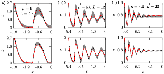
Figure 2: Generalisation of the trained functionals with chemical potential $\mu$, as expressed by Eqs. (11)–(13). Two functionals, both with $N_{1}=3$ and $N_{2}=8$ (but different $M$) are trained at $K=8$ integer values of $\mu=-2,\dots 5$, using $M_{n}=10^{4}$ particle coordinates per $\mu$-point. Top and bottom panels in (a)-(c) correspond to $M=0$ (no $\mu$ dependence) and $M=1$ (linear $\mu$ dependence). Depicted density profiles minimise (1) at the specified $\mu$ and $L$, and due to symmetry are shown for $-L/2\leq x\leq 0$. The posterior spread is illustrated by 400 samples (grey). The MAP estimators (black dots) lie close to the ground truth, $\rho_{X\mid\mu}(x)$ (red). Notice that the linear in $\mu$ model has less uncertainty, but the $\mu$-independent model has better MAP estimators, particularly in (a) and (b), where $\mu$ extrapolates from the training set. This exemplifies over-fitting.

IV Inferring the canonical functional

So far we have been considering the grand-canonical ensemble of HR. In other words, our system was open, with the number of particles fluctuating around a mean $\langle N_{\mu}\rangle$, determined by the chemical potential $\mu$. The exact cDFT of a HR fluid is known only for that case. However, there are many important problems, where one needs the free-energy functional $F_{N}[\rho]$ of a system with a fixed number of particles $N$, i.e. a canonical ensemble cDFT. For example, in non-equilibrium statistical mechanics $F_{N}[\rho]$ enters the Fokker-Planck equation for the time-dependent probability density [8, 26]. When $N$ is large, the grand-canonical and canonical ensembles are indistinguishable. But in small systems the fluctuations of $N$ may be significant, leading to large differences between the ensembles [22]. Analytically derived approximate $F_{N}[\rho]$ requires to solve systems of coupled integral equations but it is not practical due to its complexity [27]. Here we statistically infer a simple and robust approximate $F_{N}[\rho]$ from particle data.

We simulate $N$ HR by removing the particle insertion-deletion steps from the grand-canonical simulation, as described in Sec. Methods. In the canonical ensemble, the direct problem of statistical mechanics from Sec. II.1 formally looks the same. We still need to minimise $\Omega[\rho]$ in (1), with $F[\rho]\equiv F_{N}[\rho]$. There is, however, one important distinction. In the canonical ensemble, knowing the system’s partition function is equivalent to knowing the minimal $F_{N}[\rho]$ and not $\Omega[\rho]$. Consequently, $F_{N}[\rho]$ is a function of $N$, and $\Omega[\rho]$ is simply a Lagrangian of the constrained minimisation problem. Additionally, $\mu$ is no longer a thermodynamic field, but is simply a Lagrange multiplier. We can now safely proceed with the inference in Eqs. (8) and (9), where we set $\langle N_{\mu}\rangle\equiv N$. The training set $\mathcal{D}_{N}$ contains positions of $N$ particles in $K$ different pores:

$$\mathcal{D}_{N}=\{L_{n},\{\left(y_{1},\dots y_{N}\right)_{i}\}_{i=1}^{M_{n}}\}_{n=1}^{K}.$$ (14)

In Fig. 3 we plot the inference results for three different systems with small $N$. For each $L$ in (a)–(c) we trained $F_{N}[\rho]$ on 6 equispaced $L_{n}$, chosen between $L-2$ and $L+2$ with a step of 0.8, so that the test $L$ shown in the figures are not in the training sets. In each case we trained on $M_{n}=10^{4}$ particle coordinates. Black curves show the densities minimising the MAP estimators for $F_{N}[\rho]$, with the ground truth expressed by the histograms of the particle coordinates. Observe the remarkable agreement of the inferred DFT with the histograms. To highlight the difference between the ensembles in each case, we superimpose the exact grand-canonical $\rho_{X\mid\mu}(x)$, computed at $\mu$, such that $\langle N_{\mu}\rangle=N$. We notice that the ensembles differ the most in the pore centres, where $\rho_{X\mid\mu}(x)$ predicts local extrema. With further increase of the system size, the difference between the ensembles vanishes as expected.

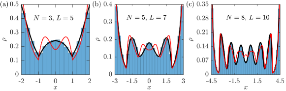
Figure 3: Out-of-sample performance of three different inferred canonical cDFT functionals $F_{N}[\rho]$, for $N$ specified in (a)-(c). In each case the same model for $F_{N}[\rho]$ is used, given by (9) with $N_{1}=N_{2}=4$. Each $F_{N}[\rho]$ was trained on a dataset in (14) with $K=6$, $M_{n}=10^{4}$, and $L_{n}$ equispaced in $[L-2,L+2]$ with step 0.8, where $L$ is specified in the figures. Black curves show $\rho(x)$ minimising the MAP estimators for the inferred $F_{N}[\rho]$. The ground truth is represented by the histograms of simulated particle coordinates at the same $L$ and $N$. Also showing the exact grand-canonical $\rho_{X\mid\mu}(x)$, computed at $\langle N_{\mu}\rangle=N$ (red). Observe the excellent agreement of the inferred canonical $F_{N}[\rho]$ with the ground truth and the break-down of the grand-canonical description of the same system.

V Data efficiency

To assess the data efficiency and accuracy of our method we compare it to a baseline black-box distributional model. Here we ignore the fact that our method yields a full cDFT functional of the underlying system and simply infer the distribution of HR. Consider the following mixture model of Gaussian radial distribution functions (RBF):

$$\rho(x\mid\mu)=\sum_{i=1}^{N_{f}}\alpha_{i}(\mu)\exp{\left(-(x-p_{i})^{2}/w_{i}^{2}(\mu)\right)},$$ (15)

where $\alpha_{i}(\mu)\geq 0$ for all $i$ and $\sum^{N_{f}}_{j}\alpha_{j}(\mu)=1$. The Gaussian means $p_{i}$ are fixed to be equispaced inside the computational domain to speed-up the training, but we assume $\mu$-dependence of the remaining free parameters in (15). As before, we consider fixed-$\mu$ and variable-$\mu$ settings, with the respective likelihoods given in Eqs. 10 and 13. For the fixed-$\mu$ model, we place a Gaussian prior on $w_{i}$ and a rectified prior distribution with mean 1 and variance 0.1 on $\alpha_{i}$, forcing $\alpha_{i}$ to be non-negative. For the variable-$\mu$ model, we treat $w_{i}$ as quadratic polynomials in $\mu$, and $\alpha_{i}$ – as an exponentiated quadratic polynomial in $\mu$. We then place Gaussian priors with zero means and variances 0.1 on the polynomial coefficients.

Figure 4 represents a comparison between the black-box and physics-informed approaches. In Fig. 4(a) we superimpose two MAP estimators in the fixed-$\mu$ setting: the RBF distribution (blue) and the DFT minimiser of the MAP functional (red dashed). Both models were trained on the same small dataset, represented by the histogram. As we saw earlier with similar examples, the physics-informed model performs very well in low-data regimes. In fact, the physics-informed $\rho(x)$ visually coincides with the ground truth $\rho_{X\mid\mu}(x)$ everywhere, and to keep the figure simple, we omitted the plot of $\rho_{X\mid\mu}(x)$. The quality of the RBF model is comparatively worse. There is simply not enough training data to produce an equally good black-box representation of $\rho_{X\mid\mu}(x)$. This is revealed by the lack of symmetry. Increasing the data size will improve the quality of the black-box model. We quantify this in Fig. 4(b) by computing the energy distance [28], $\Delta E$, between $\rho_{X\mid\mu}(x)$ and the MAP-estimators of the inference models as a function of the training data size. The physics-informed model remains at least an order of magnitude closer to the ground truth than the black-box model.

In Fig. 4(c) we compare the two approaches in the variable-$\mu$ setting. This time we superimpose the MAP estimators obtained in the regime of large training data. The data is represented by the histogram, which here visually coincides with $\rho_{X\mid\mu}(x)$. Again, the physics-informed model performs remarkably and is visually indistinguishable from the histogram. The black-box model seems to capture all the essential features of $\rho_{X\mid\mu}(x)$, but is still inferior to the physics-informed model in accuracy. A larger RBF basis may improve the representation quality in this case. The physics-informed approach yields a much more stable model and requires far fewer training $\mu$-points to achieve good representation. When extrapolating from the training set over $\mu$, both approaches may struggle for $\mu$-points far from the training set. Even when the inference becomes inaccurate, the physics-informed model would still yield symmetric distributions which satisfy statistical-mechanical sum-rules [8]. Lastly, by construction the physics-informed model generalises with $L$. We obviously cannot expect this from the black-box model. The dependence on $L$ must be explicitly built into (15), and then even more data, spanning different $L$, will be needed for training. In the end, the cost of training a black-box model may be several orders of magnitude higher than training a physics-informed model.

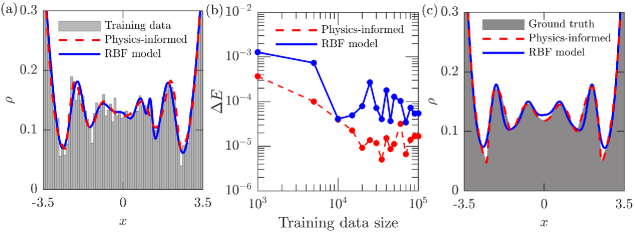
Figure 4: Comparison between the physics-informed and black-box approaches to inference. Panels (a) and (b) show fixed-$\mu$ inference, and (c) shows variable-$\mu$ inference. (a) DFT minimiser of the physics-informed model from (9) with $N_{1}=N_{2}=6$ (dashed red), and the black-box model from (15) with $N_{f}=21$ (blue). Both models are trained at $\mu=3$ and $L=8$, on the dataset in (7) of size $M=5\times 10^{3}$, represented by the histogram. (b) Energy distance [28] to ground-truth as a function of the training data size $M$. (c) Physics-informed model with $N_{1}=N_{2}=6$ (red dashed) and RBF model with $N_{f}=10$ (blue). Both are trained at $L=8$ on the dataset in (12) with $K=6$, $\mu=2.7,2.8,2.9,3.1,3.2$ and $3.3$, and $M_{i}=3\times 10^{4}$; the ground truth is shown in grey.

VI Conclusion

In the traditional sense, physical modeling is often associated with analytic derivations, followed by computation and validation against experimental data. On the other hand, modern statistical inference offers means to accomplish similar goals numerically, whilst staying in touch with the data at all stages of the modelling. Here we focused on the synthesis of both paradigms. We developed a powerful data-driven, physics-constrained approach for obtaining humanly interpretable free-energy functionals from small amounts of data. Our method is fully Bayesian and is based on uncertainty propagation through all levels of modelling yielding uncertainty quantification.

We restricted attention to a system with repulsive interactions. In a broader context, our approach can be applied to systems with more complex interactions via coarse-graining. For example, if there are long-range attractions and the repulsive free energy is obtained via inference, a simple mean-field term can be added to the functional to account for the attractions. In principle, coarse graining lets us systematically obtain different terms of the free-energy functional, corresponding to different parts of interparticle interactions. The generalisation to higher-dimensional fluids is conceptually straightforward, and can be implemented by considering functionals of the same family, $\Phi(\{n_{i}\})$. However, special care should be taken to properly train the inference model in regions, where the system undergoes phase transitions. In such cases, the parametric form of $\Phi(\{n_{i}\})$ should allow for singular behaviour.

Appendix

Simulation algorithm

Here we provide the algorithms to produce a set of particle coordinates of a HRs of radius $R$ confined inside a pore of width $L$ at chemical potential $\mu$. The steps to simulate the grand-canonical ensemble are enumerated below. The canonical algorithm for a fixed number of particles inside the same pore is obtained by repeating only steps 1-2 with $N=N_{i}$.

1. Starting with a random integer $1\leq N_{0}\leq L/2R$ (initial number of particles in the pore), do 1–3 in a loop over $i=0,1,\dots$

2. Randomly draw $N_{i}+1$ non-negative real numbers with the sum equal to $(L-2RN_{i})$. These give lengths of $N_{i}-1$ particle-particle gaps and 2 particle-wall gaps;

3. Compute coordinates $\mathcal{Y}_{i}=(y_{1},\dots y_{N_{i}})$ of $N_{i}$ particles from the gaps of step 1;

4. Obtain the new number of particles $N_{i+1}\in\{N_{i}-1,N_{i},N_{i}+1\}$ by attempting particle insertion/deletion with probabilities $P_{\text{del}}/P_{\text{ins}}$;

   $$P_{\text{del}}=\{N_{i}\exp{(-\mu)}/(L/2R)\text{ if }N_{i}>1\text{ and }0\text{ otherwise,}\}$$

   $$P_{\text{ins}}=\{(L/2R)\exp{(\mu)}/(N_{i}+1)\text{ if }N_{i}+1<L/2R\text{ and }0\text{ otherwise}\}$$ (16)

To build a set of $M$ particle coordinates in the grand-canonical ensemble, we run the steps 1–3 for approximately $ML/R$ iterations, to obtain the cumulative flattened data set $\left(\mathcal{Y}_{1},\mathcal{Y}_{2},\dots\right)$. Then we uniformly thin it to reduce correlations between $y_{i}$, keeping $M$ particle coordinates $\{y_{i}\}_{i=1}^{M}$, and compute the expected number of particles in the pore:

$$\langle N_{\mu}\rangle=\frac{1}{M_{\mu}}\sum_{i=1}^{M_{\mu}}N_{i}.$$ (17)

Log-posterior and its gradient

At a fixed $\mu$, the HMC sampler for posterior $P(Q)$ is implemented with the following expressions for log-posterior and its gradient:

$$\log{P}(Q)=\log{\mathcal{N}(Q\mid\bar{Q},\Sigma_{Q})}+\sum\limits_{i=1}^{M_{\mu}}\log{\frac{\rho(y_{i}\mid Q)}{\langle N_{\mu}\rangle}},$$ (18)

$$\nabla_{Q}\log{P(Q)}=-\Sigma_{Q}^{-1}\left(Q-\bar{Q}\right)+\sum\limits_{i=1}^{M_{\mu}}\nabla_{Q}\rho(x)\biggr{\rvert}_{x=y_{i}}\frac{1}{\rho(y_{i}\mid Q)}.$$ (19)

References

- Guyon and Wang [1994] I. Guyon and P. S. P. Wang, Advances in Pattern Recognition Systems Using Neural Network Technologies, Series in Machine Perception and Artificial Intelligence, Vol. 7 (WORLD SCIENTIFIC, 1994).
- Lake, Salakhutdinov, and Tenenbaum [2015] B. M. Lake, R. Salakhutdinov, and J. B. Tenenbaum, “Human-level concept learning through probabilistic program induction,” Science 350, 1332–1338 (2015).
- Alipanahi et al. [2015] B. Alipanahi, A. Delong, M. T. Weirauch, and B. J. Frey, “Predicting the sequence specificities of DNA- and RNA-binding proteins by deep learning,” Nat Biotechnol 33, 831–838 (2015).
- Hohenberg and Kohn [1964] P. Hohenberg and W. Kohn, “Inhomogeneous electron gas,” Phys Rev 136, B864–B871 (1964).
- Levy [1979] M. Levy, “Universal variational functionals of electron densities, first-order density matrices, and natural spin-orbitals and solution of the v-representability problem,” Proceedings of the National Academy of Sciences 76, 6062–6065 (1979).
- Evans [1979] R. Evans, “The Nature of the Liquid-Vapour Interface and Other Topics in the Statistical Mechanics of Non-Uniform, Classical Fluids,” Adv Phys 28, 143 (1979).
- Wu and Li [2007] J. Wu and Z. Li, “Density-Functional Theory for Complex Fluids,” Annu Rev Phys Chem 58, 85 (2007).
- Lutsko [2010] J. F. Lutsko, “Recent Developments in Classical Density Functional Theory,” in Adv. Chem. Phys. (John Wiley & Sons, 2010) p. 1.
- Lutsko [2019] J. F. Lutsko, “How crystals form: A theory of nucleation pathways,” Sci Adv 5, eaav7399 (2019).
- Segura, Zhang, and Chapman [2001] C. J. Segura, J. Zhang, and W. G. Chapman, “Binary associating fluid mixtures against a hard wall: Density functional theory and simulation,” Molecular Physics 99, 1–12 (2001).
- Tripathi and Chapman [2003] S. Tripathi and W. G. Chapman, “Density-functional theory for polar fluids at functionalized surfaces. I. Fluid-wall association,” The Journal of Chemical Physics 119, 12611–12620 (2003).
- Chiavazzo et al. [2014] E. Chiavazzo, M. Fasano, P. Asinari, and P. Decuzzi, “Scaling behaviour for the water transport in nanoconfined geometries,” Nat Commun 5, 3565 (2014).
- Yousefzadi Nobakht et al. [2020] A. Yousefzadi Nobakht, O. Dyck, D. B. Lingerfelt, F. Bao, M. Ziatdinov, A. Maksov, B. G. Sumpter, R. Archibald, S. Jesse, S. V. Kalinin, and K. J. H. Law, “Reconstruction of effective potential from statistical analysis of dynamic trajectories,” AIP Advances 10, 065034 (2020).
- Lin, Martius, and Oettel [2020] S.-C. Lin, G. Martius, and M. Oettel, “Analytical classical density functionals from an equation learning network,” J. Chem. Phys. 152, 021102 (2020).
- Nagai, Akashi, and Sugino [2020] R. Nagai, R. Akashi, and O. Sugino, “Completing density functional theory by machine learning hidden messages from molecules,” npj Comput Mater 6, 43 (2020).
- Chandrasekaran et al. [2019] A. Chandrasekaran, D. Kamal, R. Batra, C. Kim, L. Chen, and R. Ramprasad, “Solving the electronic structure problem with machine learning,” npj Comput Mater 5, 22 (2019).
- Percus [1976] J. K. Percus, “Equilibrium State of a Classical Fluid of Hard Rods in an External Field,” J Stat Phys 15, 505 (1976).
- Tarazona, Cuesta, and Martinez-Raton [2008] P. Tarazona, J. A. Cuesta, and Y. Martinez-Raton, “Density Functional Theories of Hard Particle Systems,” in Theory and Simulations of Hard-Sphere Fluids and Related Systems. Lecture Notes in Physics 753, edited by A. Mulero (Springer, Berlin Heidelberg, 2008) p. 251.
- Likos [2001] C. N. Likos, “Effective interactions in soft condensed matter physics,” Phys. Rep. 348, 267 (2001).
- Yatsyshin, Parry, and Kalliadasis [2016] P. Yatsyshin, A. O. Parry, and S. Kalliadasis, “Complete Prewetting,” J Phys Condens Matter 28, 275001 (2016).
- Allen and Tildesley [1989] M. P. Allen and D. J. Tildesley, Computer Simulations of Liquids (Oxford Science Publications, 1989).
- Lebowitz, Percus, and Verlet [1967] J. L. Lebowitz, J. K. Percus, and L. Verlet, “Ensemble Dependence of Fluctuations with Application to Machine Computation,” Phys Rev 153, 250 (1967).
- Wittmann, Marechal, and Mecke [2014] R. Wittmann, M. Marechal, and K. Mecke, “Fundamental measure theory for smectic phases: Scaling behavior and higher order terms,” The Journal of Chemical Physics 141, 064103 (2014).
- Zhang et al. [2020] Y. Zhang, S. Xi, A. V. Parambathu, and W. G. Chapman, “Density functional study of one- and two-component bottlebrush molecules in solvents of varying quality,” Molecular Physics 118, e1767812 (2020).
- Brooks [2011] S. Brooks, Handbook of Markov Chain Monte Carlo (Taylor & Francis, Boca Raton, 2011).
- te Vrugt, Löwen, and Wittkowski [2020] M. te Vrugt, H. Löwen, and R. Wittkowski, “Classical dynamical density functional theory: From fundamentals to applications,” Advances in Physics 69, 121–247 (2020).
- White et al. [2000] J. White, A. Gonzalez, F. Roman, and S. Velasco, “Density-Functional Theory of Inhomogeneous Fluids in the Canonical Ensemble,” Phys Rev Lett 84, 1220–1223 (2000).
- Székely and Rizzo [2013] G. J. Székely and M. L. Rizzo, “Energy statistics: A class of statistics based on distances,” Journal of Statistical Planning and Inference 143, 1249–1272 (2013).