"Drunk Man" Saves Our Lives: Route Planning by a Biased Random Walk Model

Abstract

Based on the hurricane struking Puerto Rico in 2017, we developed a transportable disaster response system "DroneGo" featuring a drone fleet capable of delivering medical package and videoing roads. Covering with genetic algorithm and a biased random walk model mimicing a drunk man to explore feasible routes on a field with altitude and road information. A proposal mechanism guaranteeing stochasticity and an objective function biasing randomness are combined. The results shown high performance though time-consuming.

Keywords Disaster Response System  $\cdot$ Genetic Algorithm  $\cdot$ K-means Clustering  $\cdot$ Proposal Mechanism  $\cdot$ K-nearest Neighbor Rule

1 Introduction

Based on the hurricane struking Puerto Rico in 2017, we developed a transportable disaster response system "DroneGo" featuring a drone fleet capable of delivering medical package and videoing roads. Assuming equal weight for both mission, we take the capability of carrying out the former missions as a constraint and a starting point from which reconnaissance routes are built.

The feasibility of fitting packages into cargo bay 1 or 2 is tested by genetic algorithm. In scenario where drones carry packages to and unloaded back, from specification of drones and loading weight can we derive the maximum reachable distance of each drone loaded. A k-means clustering algorithm is used for partitioning destinations and deriving centroids as locations of bases. Sampled points from roads are added to take into account reconnaissance mission. Points of destination are oversampled with increasing weight till centroids fall within the scope of the maximum reachable distance. Drones for each base are selected based on their performance and medical demand of destinations. Containers of each base is filled till full with minimum drones required and maximum medicine storage. Transportation of medical packages and backup drones are also included in our system.

A biased random walk model mimicing a drunk man is built to explore feasible routes on a field with altitude and road information. A proposal mechanism guaranteeing stochasticity and an objective function biasing randomness are combined. Road and home attraction are weighted differently as walk goes, to simulate the behavior of an exploratory and nostalgic drone. In modified model, we unleashed nuisance parameters to follow a log nomal distribution and use recurrent neural network to learn from previous routes and enhance its performance. The results of modified model are apparantly better and a conbination of two routes is chosen for our system. When analyzing filtered distribution of nuisance parameters and their contribution to performance, we find them neither contributing or providing reasonable experience for us to pick their values in the next run. The performance difference caused by k-nearest neighbor rule selection is huge, but the underlying mechanism is not explorable in this single field.

Table 1: Symbol Description

Symbol	Description
MPC	max Payload capacibilities of drones
MDC	max drivable capacibility of drones
k	the proportional coefficient for MDC/MPC
l	the weight of load
t	maximum flight time with cargo
T	maximum flight time without cargo
$P_{1}$	the power of flying to destination
$P_{2}$	the power of flying back
$t_{1}$	the time of flying to destination
$t_{2}$	the time of flying back
$x_{1},x_{2},\cdots,x_{n}$	the longitude of points to be clustered in K-means clustering
$y_{1},y_{2},\cdots,y_{n}$	the latitude of points to be clustered in K-means clustering
dist(X,Y)	the Euclidean distance between X and Y
$label_{i}$	point that has the least squared Euclidean distance
$a_{i}$	the centroid of each cluster
$p_{road}$	the tendency of drones flying towards roads
$p_{home}$	the tendency of drones going home
$\gamma$	relative weight of $p_{home}$
$\hat{p}_{road}$	enlarged difference of $p_{road}$
$\hat{p}_{home}$	enlarged difference of $p_{home}$
$\alpha$	constant relevant to $\gamma$
$\beta$	constant relevant to $\gamma$
MFD	maximum flight distance
d	distance from current cell to the origin
CNN	convolutional neural network
RNN	recurrent neural network
t-1,t,t+1	a Time-Series data set
X	input data set
W	input weight
U	weight of sample in this time
V	output weight
CCR	conbinational coverage rate
NC	net coverage
A	the area of a specified bounding box
$\hat{f}(x)$	indicates the distribution function of after filtering
$f(x)$	indicates the distribution function of before filtering
$m(\hat{f}(x))$	measure of $\hat{f}(x)$. from measure theory to probability theory.
$m(f(x))$	measure of $f(x)$, from measure theory to probability theory.

2 Introduction

2.1 Symbol Description and Disambiguity

2.1.1 Symbol Description

For symbol description, see table 1.

2.1.2 Disambiguity

1. A base is where container is located and drones depart. Bases store medicine and retrieve drones to process videos for decision-making.

2. A destination is where medical package is delivered to.

3. A package plan of destination A is all the medical packages needed by destionation A in a day.

4. Word "feasible" has different meanings: feasible base means drones that depart from it could reach the destination; feasible drone plan means the packages can be packed into the drone cargo bay; feasible cell means drone can walked on it for reason defined in context; feasible route means the drone goes back home in the end.

5. Field: The place where our drone walks on. It has all the factors perceptible and necessary to our drone.

6. Road coverage: the sum of the importance of cells on the route, used for route evaluation.

2.2 Problem Restatement

The occurance of natural disaster events recorded has been increasing exponetially since 1900, despite the recent minor decline [1]. The horrific casualty and economic damage caused by catastrophes concerns every Earth citizen who dreams about living a safe and comfortable life. Not only does timely and adequete response to natural disasters helps decrease casualty and property loss, but also it reassures people from anxiety in the context of global climate change.

Required by HELP, Inc., we developed a transportable disaster response system, "DroneGo", based on the hurricane that struck Puerto Rico in 2017. It includes a drone fleet and medicine configurated according to anticipated medical package demand of destination. It’s carried in ISO standard cargo containers and transported to elaborately picked bases from which drones depart with two missions — medical package delivery and video recording.

2.3 Our Work

We divided the ultimate goal into two sub-problems:

• Selecting base locations and drones and making delivery plan.

• Making reconnaissance routes.

In the first problem, locations are given by k-means clustering of oversampled delivery locations and sampled points on main roads. The maximum reachable distance of different drones are calculated in the scenario that drones carry packages when flying to the delivery locations and are unloaded when going back. The maximum flight time under specific loading weight is derived from a linear model according to max payload capability and flight time with no cargo given by attachment 2. All combination of drones and package plans 3 are numerated and tested by a genetic algorithm for whether they can be packed into the drone cargo bay. The flight capabilities of drones serve as constraints to our k-means clustering in a way that the oversampling weight of delivery points increases till each cluster centers fall within the overlapping scope of maximum reachable circle of destinations. The most requirement-satisfactory drones are selected based on the performance and missions assigned.

In the second problem, we prototyped initial feasible routes by simulating a biased random walk model on a raster featuring altitude and importance derived from the place main roads are located. A proposal mechanism is used to move drones from current cell to a randomly-picked adjacent available cell. Drones decide whether to accpet or reject the proposal based on an objective function of importance and distance from the starting cell. In optimization stage, we integrated feasible and well-performed routes into the objective function, weaken bias by recurrent neural network and unleashed hard-coded parameters by specifying them to follow a lognormal distribution. We also combined 2 routes to get higher coverage to elevate the reconnaissance ability of our system.

2.4 Assumptions

1. When departing for delivery mission, drones first rise to the height required for the route; When landing, drones move right above the spot then go straight down. Time for going straight up and down is negligible.

2. Drones carry out missions seperately.

3. When filming, drones keep at a specific height above ground to keep the resolution of videos.

4. The maximum distance from which roads can be filmed is $50m$.

5. Only bases have charging facilities for drones.

6. One flight has only one destination and the drone carries all the medical packages the destination needs for a day.

7. Maximun flight time decreases linearly with the total weight of cargos with coefficient $k\leq 1.3$.

8. Drones’ speed is constant, regardless to cargo weight.

9. The weight of buffering material can be ignored.

10. Medicine would not go bad, therefore we should fill the container with as many medical packages as possible.

3 Data Manipulation

3.1 Data Source

We obtained a georeferenced raster image displaying elevation data for Puerto Rico and the U.S. Virgin Islands derived from NED data released in December, 2010[3]. The data is in $100\,m\times 100\,m$ resolution and uses the Albers Equal-Area Conic projection.

Road shape data is from OpenStreetMap, a open data licensed under the Open Data Commons Open Database License (ODbL) by the OpenStreetMap Foundation (OSMF)[2]. Thanks to thousands of individuals who contributed to the database.

3.2 Data Wrangling

We cropped the altitude raster into a $700\times 1900$ extent, covering the entire mainland of Puerto Rico. World Geodetic System (WGS84) is the coordinate reference system to which the raster is projected to acquire the longitude and latitude of cells.

We filtered out minor roads in shape files to include only motorways, divided roads, national roads and regional roads. To transform shape files to one single raster for our drones to walk on, we buffered lines with $50\,m$ radius4 and masked a template raster with derived polygons. For each road types, we assigned a progressively decreasing series $(2,\sqrt{3},\sqrt{2},1)$ as their importance and picked the highest importance if one cell belongs to more than once type.

To integrate altitude and road data, we stacked them to a brick file with the same extent and CRS as one of the input data of our model.

4 Part1: Container Configuration

4.1 Analysis of the problem

We came up with three considerations when choosing the best location for bases:

• Drones should be able to fly from the base to distination with medicine and come back unloaded;

• Drones can fly from one base to another to make up for medicine shortage.

• The number of roads that drones can monitor, measured by the number of cells of roads;

All three factors involves calculation of maximum flight distance of drones carrying medical packages, which should be thought about first. Because we don’t consider time and energy consumption, if the base is feasible for delivering medicines, the actual distance between the base and destination is ignored when scheduled. In reality, this could be compensated by forcing drones to deliver packages at night because daytime is more valuable for reconnaissance.

After bases are determined, drones could be selected according to performance and the medicine demand of distination. When filling containers, we first decided the type and number of drones. Then the medical packages are filling into the rest space of the container in a given proportion till the container is full.

Due to the fact that one base may have too many destinations, and thus medical packages are consumed much faster than other bases, we considered making it possible to deliver medical packages from one base to another or to share drones between bases to save space.

4.2 Maximum Distance Calculation

Max payload capability $(MPC)$ mentioned in attachment 2 is redefined as the maxinum capability in which condition are in safety-guaranteed condition, and we defined an imaginary max drivable capability $MDC=k\cdot MPC$, in which condition are not able to fly, where $k$ is the proportional coefficient.

Maximum flight time with cargo $t$ is in negative relationship to cargo weight $l$.Therefore, under any load $l$, the maximum flight time can be derived as:

$$t=-\frac{T}{MDC}\cdot l+T,$$ (1)

where T is the maximum flight time without cargo.

The power of flying to and back is different but time consumption of flying to and back is the same. In a round trip that approaches the farthest spot, total energy storage $E$ of a drone is used up:

$$P_{1}\cdot t+P_{2}\cdot t=E,$$ (2)

where $P_{1}$ is the power of flying to, $P_{2}$ is the power of flying back, and $t$ is the time consumption of flying to or back:

$$t_{1}=t_{2}=\frac{D}{2V},$$ (3)

where $D$ is the maximum reachable distance, and $V$ is the speed constant. The power of flying to and back can be derived from division of energy and time:

$$P_{1}=\frac{E}{t_{1}}=\frac{E}{-\frac{T}{MDC}\cdot l+T}$$ (4)

$$P_{2}=\frac{E}{t_{2}}=\frac{E}{T}$$ (5)

Finally we subsituted equation (4,5) into equation (6) and derived maximum reachable distance $D$ under load $l$:

$$D=\frac{l-k\cdot MCP}{l-2k\cdot MCP}\cdot\frac{V\cdot T}{30}$$ (6)

4.3 Cargo Bay Filling

A genetic algorithm is used for this 3-D bin packing problem. We first enumerated all the combination of drones and package plans and then tested for feasibility of packing the package plan into the cargo bay. Here are the feasible drone package plans for each destination. Only top two plans with longest distance for each destination is shown.

Table 2: Feasible drone plan with $k$ arbitrarily set as 1.3

Destination	Drone	Bay Type	MED1	MED2	MED3	Weight	Distance
Caribbean Medical Center
Fajardo	B	1	1	0	1	5	36
Caribbean Medical Center
Fajardo	C	2	1	0	1	5	31.39
Hospital HIMA
San Pablo	C	2	2	0	1	7	28.44
Hospital HIMA
San Pablo	F	2	2	0	1	7	27.19
Hospital Pavia Snturce
San Juan	B	1	1	1	0	4	40.13
Hospital Pavia Snturce
San Juan	C	2	1	1	0	4	32.72
Puerto Rico Children’s Hospital
Bayamon	F	2	2	1	2	12	23.21
Puerto Rico Children’s Hospital
Bayamon	C	2	2	1	2	12	18.97
Hospital Pavia Arecibo
Arecibo	B	1	1	0	0	2	47.06
Hospital Pavia Arecibo
Arecibo	C	2	1	0	0	2	35.16

4.4 Oversampling and K-means Clustering Model

Since the packing problem is simply organized, our focus is the location(s) of cargo container(s). We firstly oversampled the locations of hospitals due to the minority of hospitals compared with roads, and then we located the cargo containers by K-means to cluster.

Oversampling in data science is a technique, that is used to adjust the class distribution of a data set. The number of points from the road greatly exceeds the number of locations of hospitals, which leads to an imbalance in the data set. In details, if we give them the same weight to calculate the best locations, the result would certainly ignore the tiny turbulence of the locations of hospitals. Therefore, we decided to oversample the locations of hospitals by giving them more weights to emphasize the importance of hospitals. After oversampling, we used K-means clustering to classify three categories of hospitals and main roads, and find the K-means centers of three categories.

We conducted the algorithm of K-means clustering. Here, euclidean distance formula is defined as:

$$dist(X,Y)=\sqrt{\sum_{i=1}^{n}\left|x_{i}-y_{i}\right|^{2}}$$ (7)

Let $T=x_{1},x_{2},\cdots,x_{m}$ be the points to be clustered. The steps of k-means clustering are as follows:

1. Initialize $k$ cluster centers $a_{1},a_{2},\cdots,a_{k}$;

2. Assign each point to the cluster whose mean has the least squared Euclidean distance.

   $$label_{i}=\mathop{\arg\min}_{1\leq j\leq k}{\sqrt{\sum_{i=1}^{n}(x_{i}-a_{j})^{2}}}$$ (8)

3. Recalculate the centroid of each cluster given as:

   $$a_{i}=\left(\frac{\sum_{j}^{n}x_{j}}{n},\frac{\sum_{j}^{n}y_{j}}{n}\right)$$ (9)

4. Check if it meets a terminal condition, which could be evaluated by iteration times, mean squared error or cluster center varying frequency.

5. Go to step 2.

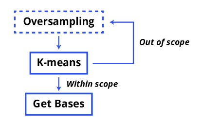
Figure 1: K-means

In the realistic occasions, we see that the ratio of the number of hospitals and the number of sampled points on main roads are over 1:10, so we decided to oversample the number of hospitals into a ratio of 1:1. Then we put these points into K-means clustering, which would give back $k(1\leq k\leq 3)$ cluster centers back. To determine $k$, we prints three possible results of $k$. In the occasions of $k=1,2$, distances from cluster centers to hospitals are too long for drones to arrive by its limited batteries, according to Table 2. So we had to locate 3 cargo containers as the DroneGo disaster response system.

The result of k-means clustering, which indicates the locations of cargo containers, is (18.3147,-66.8219), (18.298,-66.2065), (18.2698,-65.7574). The locations of cargo containers and sampled points on main roads are shown as figure 2.

Five destinations can be partitioned into 3 clusters:

• Base 1: Caribbean Medical Center

• Base 2: Hospital HIMA , Hospital Pavia Snturce and Puerto Rico Children’s Hospital

• Base 3: Hospital Pavia Arecibo

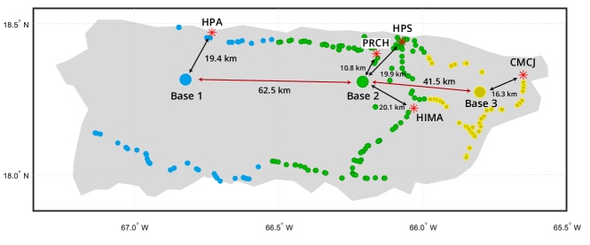
Figure 2: K-means Result

Base 1 and 3 have only one destination assigned and the optimal drone shown in table 2 for both bases are drone B. Thus drone B is our choice for base 1 and 3 with no doubt.

Base 2 has three destinations assigned, and the most optimal common drone of those three destinations is drone C (ranked first in Hospital HIMA, second in both Hospital Pavia Snturce and Puerto Rico Children’s Hospital). Therefore drone C should be chosen for delivery mission for base 2.

For reconnaissance, drone B is outstanding in terms of maximum flight distance (53 km), so each base should at least has one drone B for filming roads. Even though drones have service life more than 2 years, we still decided to double the drone numbers in case that accidents happen. Two drone H are also included for each base for communication purpose.

Because the distance between base 2 and 3 is 41.5km and is lower than either the maximum reachable distance of drone B carrying MED1 or without loading, we considered transportation of medical packages between base 2 and 3. By moving all MED1 storage from base 2 to base3, we can even the medical package number ratio. The rest space of the container is filled with medical packages in the proportion specified by destination medicine demand. The actual number of each medical package in each base is calculated by genetic algorithm metioned in 4.3. Our container configuration is shown as follows:

Table 3: Packing configuration for cargo containers

Base	Distination	Drone Config	Drone of Delivery	MED 1	MED 2	MED 3	Supporting Days
1	HPA	B$\times$4 H$\times$2	B	2251	0	0	375
2	HIMA HPS PRCH	B$\times$2 C$\times$2 H$\times$2	C	0	1080	2160	375
3	CMC	B$\times$2 H$\times$2	B	1320	0	1320	1320

We visualized the packing configuration of each package plan (figure 3).

Figure 3: Drone playload packing configurations

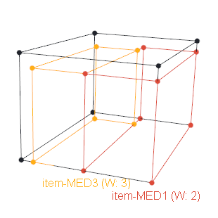
(a) Drone B with MED1,3

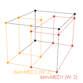
(b) Drone B with MED1,2

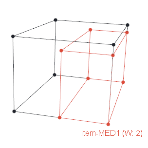
(c) Drone B with MED1

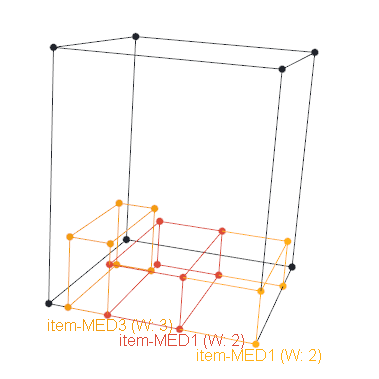
(d) Drone C with MED1,1,3

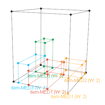
(e) Drone C with MED1,1,2,3,3

5 Part2: Route designing by Biased Random Walk Model

5.1 Analysis of Problem

In previous section, we decided the drone type for each base. All three bases have drone B, which can also fly farther than any other drones and has the video capability. Therefore, it’s our perfect choice for reconnaissance.

When we thought about the problem, we first come up with a deterministic model of path searching. However, deterministic model has its own flaws:

• It’s easy to be trapped in a regional optima.

• It depends too much on some arbitrary parameters.

• It only gives one feasible route. If accidents happen, namely wildfire, and block some cells, the entire route is not applicable anymore.

• It can not amend the route automatically when trapped in dead ends.

Thus, we decided to build a stochastic model simulating a random walk of "drunk man" with the following advantages:

• It’s expected to explore all feasible routes and thus find the global optima for us.

• It’s naturally compatible to stochastic parameters. Thus, our biased walk is less biased by human discretion and more affected by the environment.

• It gives many feasible routes, many of which are equally good. The alternative routes are good backup routes.

• We don’t have to consider how to design a feasible route because we can easily abandon infeasible routes.

We use the metaphor of a drunk man to blueprint our model. Our drunk man should behave as follows:

1. Biased: attracted by roads;

2. Exploratory and nostalgic: moving apart from the origin in the beginning and come back home in the end;

3. New-trumps-old mindset: reluctant to walk on roads that it has walked on previously.

Accordingly, our drunk man should sense the following factors:

1. Importance: evaluated by road type.

2. Altitude change: drones fly at the same height from ground.

3. Moving distance: drones should go back to base before it’s running out of power.

After sensing the necessary factors, our drunk man can finally take the first step! But it still needs to integrate all those factors. But it’s in its mind, anyway. Let’s see how it works.

5.2 Preliminary Model

5.2.1 Random Walk Procedure

Imagine on Christmas eve a man gets loaded for some reason. It has nothing to do. Why not take a walk? So it decides to wander around the field. Departing from home, sometimes it would explore off the roads, but as a sane man, it would keep speeding as much time as possible on roads. Here is what’s going on in its mind: First, it looks around and randomly pick a place to step on. It’s not a psychopath at least so it would avoid hitting a tree or fall into rivers. After spotting a place, it would stare at it for a while to evaluate the spot it chose. Then it accept or reject the spot based on its evaluation. Keep in mind it’s drunk so it’s likely that it would be willing to accept a spot deviating from the main road. But the man has a good memory even when unconscious, so it would avoid going to the place once again (but is not compulsory). After moving to a new spot, it repeats the previous steps.

In parallel universes, sometimes our drunk man would fall into some trenchs (scenario 1); sometime it would get exhausted (scenario 2); but sometimes the man finally get home (scenario 3)! That’s a good news, and the track of its walk is what we are looking for.

It’s time to implement our drunk man in algorithm. First of all, we initalized the drone sited on our bases. The drone keeps iterating the following steps on the field till one of three scenarios mentioned above happens.

1. Search for all available adjacent cells, generate a random number and propose one of them according to a uniform probability;

2. Evaluate the proposed cell by an objective function; which should gives a value between 0 to 1;

3. Decide whether to accept or reject the proposal. Generate another random number for making decision. If lower than the value in step 2, it accepts the proposal, decrease the importance of the adjacent cells and moves to the proposed cell. If it’s lower, it rejects the proposal and keeps still.

5.2.2 Objective Funcion

The objective function integrates all information necessary to our model and is the only source affecting drones’ tendency of filming road networks or going home. It evaluate the relative superiority of proposed cell to other adjacent feasible cells.

We supposed three elements, $p_{road}$, which affects the tendency of drones flying toward roads, $p_{home}$, which affects the tendency of drones going home, and $\gamma$, which is the relative weight of $p_{home}$. The value $f$ of objective function is given as:

$$f=p_{road}+\gamma\times p_{home}$$ (10)

Let $p_{road}=\frac{road_{i}}{\sum road_{i}}$, and $p_{home}=\frac{home_{i}}{\sum home_{i}}$, where $road_{i}$ means the significance of selected point by K-nearest neighbor rule (described later), and $home_{i}$ means the distance from the selected point to the origin. Here, $p_{road}$ and $p_{home}$ are nondimensionalized by other feasible cells adjacent to the current cell, so that $\sum p_{road}=\sum p_{home}=1$, and therefore $p_{road}$ + $p_{home}$ is plausible. We enlarge the difference between $home_{i}$ and $road_{i}$ by exponetialization. Thus, let

$$\hat{p}_{road}=\frac{e^{road_{i}}}{\sum e^{road_{i}}},\quad\hat{p}_{home}=\frac{e^{home_{i}}}{\sum e^{home_{i}}}$$

Still, $\hat{p}_{road}$ and $\hat{p}_{home}$ are nondimensionalized.

To make our drone exploratory and nostalgic, we defined the relative weight of home attraction $\gamma=\alpha\times(d/MFD-\beta)^{3}$ where $\alpha=0.2\&\beta=0.3$ are set arbitrarily, $d$ is the distance from current cell to the origin and $MFD$ is maximum flight distance, $MFD=53000$ for drone B. $\gamma$ is negative at the beginning of the route, making cells apart from the origin have higher probability to be accepted. When leaving origin for some distance, $\gamma$ is close to zero and $p_{road}$ takes major place in accpeting or rejecting proposed cells. In this period the drone behaves totally based on road attraction. In final stage when flight distance is approaching $MFD$, $p_{home}$ is in charge of the process and the drone would accept proposed cells directing to the origin with higher probability.

The sensing range of the drone is specified by the K-nearest neighbor rule. When larger neighbor rule is used, the drone is able to be attracted to remote roads if the drone is wandering within a non-road space. However, if roads are more dense in the field, it’s possible that the heterogeneity of the field is blurred out and thus the drone that moves along roads in small rule would move unintentionally. In this paper, Four|eight|twelve-nearest neighbor rules are implemented in our program and the results are discussed in sensitive analysis.

(f) Four-nearest neighbor rules

(g) Eight-nearest neighbor rules

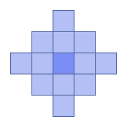
(h) Twelve-nearest neighbor rules

Figure 4: K-nearest neighbor rule

5.2.3 Results of Preliminary Model

After letting off 10000 drones, we picked the route with the highest coverage and ploted in 6. As we can see, in fig a, the drone spent too much time off roads and wandering on the left-bottom corner of the picture. It depicts that roads are not attracted by roads to enough extent. In fig b, the drone covers some part of the nearest road but fail to move farther to explore more territory. Therefore, we concluded $\gamma$ is too small in both ends. Besides, the field is discontinuous at most parts, therefore unbiased walk is commonly expected when drones are trapped in a non-road field. Therefore, some irrational looping is inevitable.

5.3 Modified model

5.3.1 Unleashing Parameters

In defining the relative weight of home attraction $\gamma$, two nuisance parameters $\alpha\&\beta$ are used:

$$\gamma=\alpha\times(d/MFD-\beta)^{3}.$$

$\beta$ determines when $\gamma=0$ and thus pinpoints the turning point of drones from exploratory (going out) to nostalgic (going back). After rescaled by $\alpha$, the $\gamma$ is increased or decreased, making home attraction more or less important in proposal mechanism.

We modified our model by unleashing those two parameters from our hand. We set $\alpha$ and $\beta$ to follow a log normal distribution with means equal $0.5$ and $0.5$ respectively and variance equal $0.7$ and $0.05$ respectively. Those numbers are derived arbitrarily. According to previous analysis, $\gamma$ is small in both direction, we elevated the mean of scalar $\alpha$. After we simulated a feasible route, we would take down its $\alpha\&\beta$ and distance for further analysis.

5.3.2 Experience Learning

Importance data is naturally discrete but experience of previous drones is not. If we use Convolutional Neural Networks(CNN), it cannot memorize the former choices. In order to fit our biased random walk model, we should set a neural network that can memorize the former choices and decide its next move with the turbulance of former choices.

Here we introduce Recurrent Neural Network(RNN). RNN can make use of a sequential information, which means that RNN can memorize former choices and decide its next move by some kind of weight of former choices. In our case, according to our Biased Random Walk Model, we choose the furthest distance that drones go, the repeated routes that drones have, and the standard deviation as our parameters into RNN, trying to train more stable and more accurate parameters into the previous model.

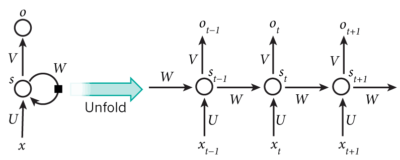
Figure 5: The principle of the recurrent neural network[13]

The figure 5 is the unfolded picture of Hidden Layer of RNN. $t-1,t,t+1$ depicts a Time-Series set, X means the input data set, $S_{t}$ means the memory of sample situated in the time $t$, $S_{t}=f(W*S_{t-1}+U*X_{t})$, where $W$ means the input weight, $U$ means the weight of sample in this time, $V$ means the output weight.

When $t=1$, we initialize $S_{0}=0$, randomly initialize $W,U,V$, and calculated by the equations below:

$$h_{1}=U\dot{x}_{1}+W\dot{s}_{0}$$

$$s_{1}=f(h_{1})$$

$$o_{1}=g(Vs_{1})$$

where function f and function g are both activation function, f can be classic tanh, relu and sigmond function, g can be softmax function. When $t=2$,

$$h_{2}=U\dot{x}_{2}+W\dot{s}_{1}$$

$$s_{2}=f(h_{2})$$

$$o_{2}=g(Vs_{2})$$

As shown above, we can deduce the general equation from this:

$$h_{t}=U\dot{x}_{t}+W\dot{s}_{t-1}$$

$$s_{t}=f(h_{t})$$

$$o_{t}=g(Vs_{t})$$

In our Random Walk model, we remembered the former state and then made its next move. Training the model by RNN, can enhance performance of our model.

Figure 6: The results of preliminary model

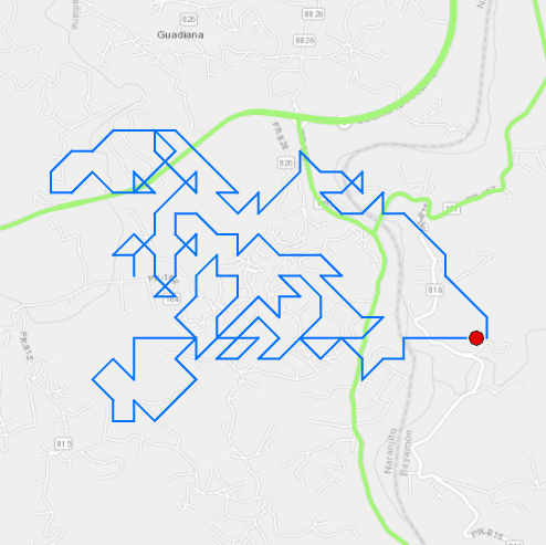
(a) Route 1

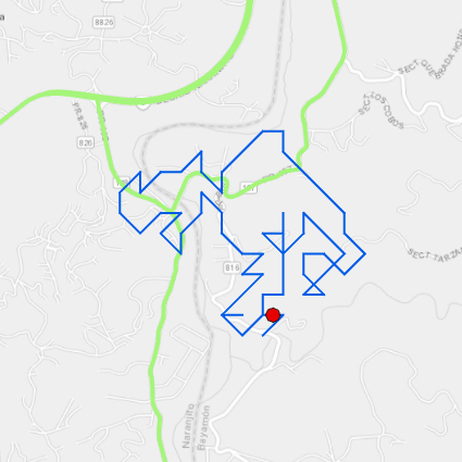
(b) Route 2

Figure 7: The results of modified model

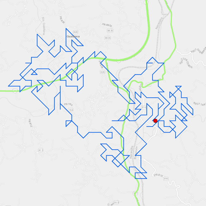
(a) Route 3

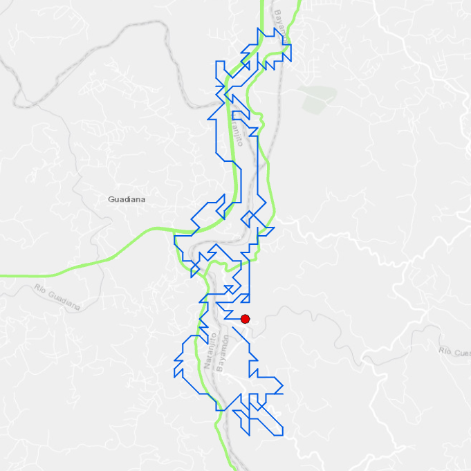
(b) Route 4

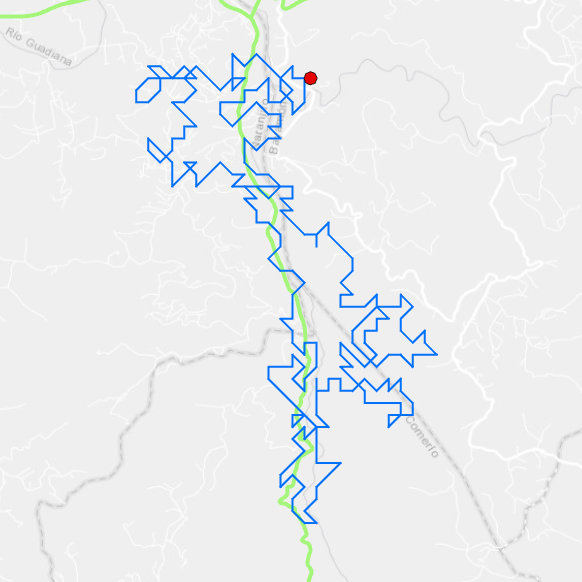
(c) Route 5

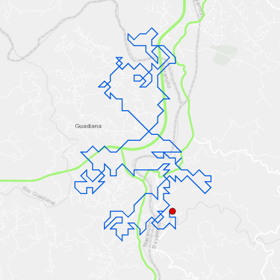
(d) Route 6

5.4 Results of Modified Model

The results of modified model are plotted in fig 7 from a to d. As we can see, those routes are significantly better than results of preliminary model. For example, the drone of route in figure 8(a) walked along roads for a long distance and crossed the non-road field as if roads on the right botton corner are pulling it. However, some small loops still exists in all four routes.

For better coverage, we tried to overlay 2 routes chosen from all feasible routes. Conbinatorial Coverage Rate(CCR) is derived from $CCR=\frac{NC}{A}$, where $NC$ is the net coverage defined as the coverage of union of two routes, and $A$ is the area of a specified bounding box.

Combination of route in figure 8(a) and 8(b) has the highest conbinatorial coverage rate (0.82) among all possible plans.

6 Sensitivity Analysis of Model

6.1 Distribution Change of Behavior Parameters

In modified model, we unleashed behavior parameters $\alpha$ and $\beta$ to follow a lognormal distribution. If we only save the value of those two parameters of routes whose coverage surpasses some threashold, our model could be seen as a gate that filters out some paramters that are not "fittable" intuitively for (1) generate a feasible route (2) increase the coverage.

First, we did a regression analysis of $\alpha$ and $\beta$ to coverage. However, there is no significant relationship between any two of them (figure 8). Second, we did a lognormal fitting of $\alpha$ and $\beta$ respectively (figure 9). $\alpha$ still fits a lognormal distribution($R^{2}=0.89$), with consistant mean value and a small deviation of variance from $0.7\to 0.61$. In terms of $\beta$, it fails to fit a lognormal distribution and has the mean value $0.43$ and variance $0.29$.

Figure 8: Regression analysis of $\alpha$ and $\beta$

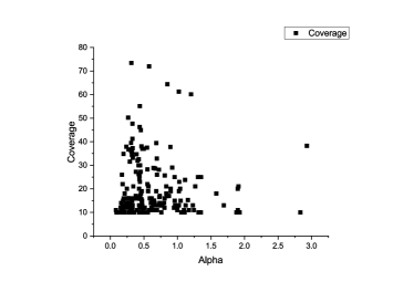
(a) Alpha

(b) Beta

Figure 9: Lognormal fitting of $\alpha$ and $\beta$

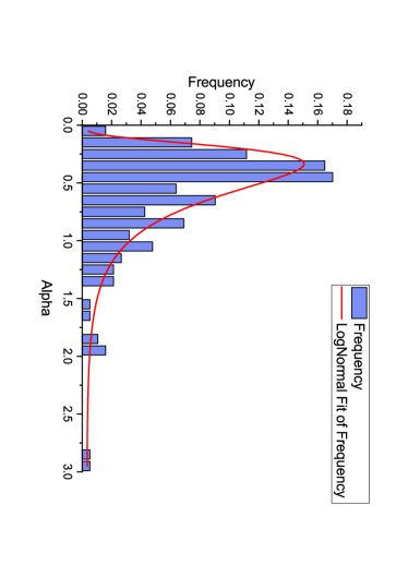
(a) Alpha

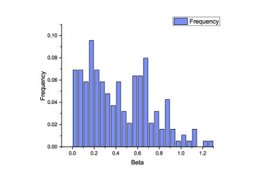
(b) Beta

This analysis shows that neither $\alpha$ or $\beta$ has contribution to the performance of the biased random walk process. The distribution of $\alpha$ is not significantly affected after filtering. However, the distribution of $\beta$ is evened.

$$\hat{f}(x)=\left\{\begin{aligned} g(x)<f(x),x\in K\\ f(x),x\notin K\end{aligned}\right.K\in U(\mu,\epsilon);$$ (11)

So, we can get that,

$$M[\hat{f}(x)]=M_{x\in K}[\hat{f}(x)]+M_{x\notin K}[\hat{f}(x)]=M_{x\in K}[g(x)]+M_{x\notin K}[f(x)]\leq M[f(x)]$$

which means that the probability of after filtering is smaller than the prob

$\beta$ has explicit meaning in our model — time when home attraction surpasses road attraction. Intuitively we expect our drone to turning from departing to going back in the halfway. However, this expectation is probably flawed according to our result. A drone either tending to move near its origin or go far away is probably more likely to make a feasible route and has higher coverage. It occurred to our mind that maybe the lognormal distribution is not a good distribution for our nuisance parameters. And even distribution would generate a more interpretable distribution for results because it’s not skewed at the beginning. However, even distribution is not an uninformative distribution[14], and thus it will still affect the result.

6.2 Performace Change due to K-nearest neighbor rule

We conducted our model based on different K-nearest neighbor rule. The 8-nearest neighbor rule performs best according to average distance and coverage, and 4-nearest neighbor rule worst. The relationship between rule and performance is not deterministic. Field heterogeneity plays a key role. Therefore, we cannot interpret anything from results of a single field. More artificial field should be generated for further analysis.

7 Stength and Weakness

7.1 Strength

1. We used real data for analysis and correctly projected points based on coordinate reference system.

2. We used stochastic model to generate feasible routes to minimize anthropogenic bias underlying evaluation method.

3. The model is space-explicit — it uses as much spatial data as possible to reflect the reality. No simplication on data side is applied apart from importance assignment of roads.

4. This model is flexible that many parts could be modified to integrate new factors biasing our route designing.

7.2 Weakness

1. We have no idea how to tradeoff between delivery distance and road coverage so we arbitrarily emphasized the latter, which may be seen as penny wise and pound foolish.

2. We simulate one drone at a time. Therefore, the combination of routes would have too many overlapping parts.

3. The behavior of our drone is uncontrollable. For example, local looping of routes are inevitable. Afterwards smoothing is required.

4. The algorithm is time-consuming and even though does not guarantee to find the best solution.

5. The initial distribution of nuisance paramters still has some arbitrariness, and filtered distribution is not interpretable.

References

- [1] Hannah Ritchie and Max Roser. Our World in Data, Natural Disasters. In https://ourworldindata.org/natural-disasters, 2019.
- [2] OpenStreetMap contributors. Planet dump retrieved from https://planet.osm.org. In https://www.openstreetmap.org, 2019.
- [3] Geological Survey (U.S.) 100-Meter Resolution Elevation of Puerto Rico and the U.S. Virgin Islands, Albers projection In National Atlas of the United States, 2010.
- [4] Li, Xueping and Zhao, Zhaoxia and Zhang, Kaike A genetic algorithm for the three-dimensional bin packing problem with heterogeneous bins In IIE Annual Conference. Proceedings, Page 2039, Institute of Industrial and Systems Engineers (IISE), 2014.
- [5] Christopher Olah Understanding LSTM Networks In http://colah.github.io/posts/2015-08-Understanding-LSTMs/, 2015.
- [6] Martello, Silvano and Pisinger, David and Vigo, Daniele The three-dimensional bin packing problem In Operations Research, Page 256–267, 2000.
- [7] Themistocleous, Kyriacos The use of UAV platforms for remote sensing applications: case studies in Cyprus In Second International Conference on Remote Sensing and Geoinformation of the Environment (RSCy2014), International Society for Optics and Photonics, 2014.
- [8] Wu, Yong and Li, Wenkai and Goh, Mark and de Souza, Robert Three-dimensional bin packing problem with variable bin height In European journal of operational research, 2010.
- [9] Daniel, Kai and Dusza, Bjoern and Lewandowski, Andreas and Wietfeld, Christian AirShield: A system-of-systems MUAV remote sensing architecture for disaster response In Systems conference, 2009 3rd Annual IEEE, 2009.
- [10] Yu, Chaoqing and Lee, JAY and Munro-Stasiuk, Mandy J Extensions to least-cost path algorithms for roadway planning In International Journal of Geographical Information Science, 2003.
- [11] Kitjacharoenchai, Patchara and Ventresca, Mario and Moshref-Javadi, Mohammad and Lee, Seokcheon and Tanchoco, Jose MA and Brunese, Patrick A Multiple Traveling Salesman Problem with Drones: Mathematical model and heuristic approach In Computers & Industrial Engineering, 2019.
- [12] Saha, Ashis Kumar and Arora, Manoj K and Gupta, Ravi Prakash and Virdi, ML and Csaplovics, Elmar GIS-based route planning in landslide-prone areas In International Journal of Geographical Information Science, 2005.
- [13] LeCun, Yann and Bengio, Yoshua and Hinton, Geoffrey Deep learning In Nature Publishing Group, 2015.
- [14] Gelman, Andrew and Stern, Hal S and Carlin, John B and Dunson, David B and Vehtari, Aki and Rubin, Donald B Bayesian data analysis In Chapman and Hall/CRC, 2013.