Numerical scheme for the far-out-of-equilibrium time-dependent Boltzmann collision operator: 1D second-degree momentum discretisation and adaptive time stepping

Abstract

Study of far-from-equilibrium thermalization dynamics in quantum materials, including the dynamics of different types of quasiparticles, is becoming increasingly crucial. However, the inherent complexity of either the full quantum mechanical treatment or the solution of the scattering integral in the Boltzmann approach, has significantly limited the progress in this domain. In our previous work we had developed a solver to calculate the scattering integral in the Boltzmann equation. The solver is free of any approximation (no linearisation of the scattering operator, no close-to-equilibrium approximation, full non-analytic dispersions, full account of Pauli factors, and no limit to low order scattering) Michael . Here we extend it to achieve a higher order momentum space convergence by extending to second degree basis functions. We further use an adaptive time stepper, achieving a significant improvement in the numerical performance. Moreover we show adaptive time stepping can prevent intrinsic instabilities in the time propagation of the Boltzmann scattering operator. This work makes the numerical time propagation of the full Boltzmann scattering operator efficient, stable and minimally reliant on human supervision.

I Introduction

The study of ultrafast dynamicsFujimoto1984 ; Elsayed1987 ; Schoenlein1987 ; Brorson1990 ; Fann1992 ; Hertel1996 ; Fatti2000 ; Stamm2007 has allowed for the discovery of a number of very interesting effectsBeaurepaire1996 ; Terada2008 ; Crepaldi2012 ; Garcia2011 ; Cacho2015 ; Battiato2018PRLHalfMetals ; Cheng2019 ; Wang2018THzTopolInsul ; Lindemann2019UltrafastSpinLasers . Its theoretical description however has to face a number of challenges, since the most interesting effects often come from the interplay of laser excitation, thermalisation of different types of quasiparticles and transportmalinowski2008control ; battiato2010superdiffusive ; rudolf2012ultrafast ; kampfrath2013terahertz ; eschenlohr2013ultrafast ; battiato2016ultrafast ; Freyse2018 . The concomitant description of these different effects is further aggravated by the fact that out-of-equilibrium dynamics dramatically increases the complexity, as the population cannot be anymore safely assumed as close to equilibriumBagsican2020THzCNT . The large amount of degrees of freedom required to describe a band, position and momentum dependent population increase vastly any theoretical and numerical effort. It is also evident that at times the need to describe several types of quasiparticles requires input from a number of methods, further increasing the complexity. Finally, all these data about transport and scattering for different quasiparticles need to be integrated into a single treatment.

The time dependent Boltzmann equation (BE)Boltzmann1872 has proven very powerful in tackling this complexity as it allows for a seamless integration of transport and scattering even among different types of quasiparticles Semiconductor1969 ; cercignani1988boltzmann ; Abdallah1996 ; Mahan2000 ; Choquet2000 ; Rethfield2002 ; Majorana2004 ; Caceres2006 ; Snoke2011 ; Tani2012 ; Vatsal2017 ; wais2018quantum . This approach requires the tackling of two fundamental issues. First, the BE needs ab initio input for the dispersions and the scattering matrix elements. While finding dispersions for quasiparticles is nowadays routine work in many cases, the second part is far more challenging, yet recently it has been successfully tackled for different quasiparticles by several groups jhalani2017ultrafast ; li2014shengbte ; lindsay2014phonon (we do not address this issue here). The second issue, which we address in this work, is the discretisation of the time-dependent BE itself, after the ab initio input is known.

The BE has been widely used in a range of fields spanning from gasses, plasma, and semiconductor’s physics (we focus here specifically on the time-dependent equation)colonna2016plasma ; villani2002review ; kremer2010introduction ; saint2009hydrodynamic ; colussi2015undamped ; snoke2011quantum ; shomali2017monte ; xu2017lattice . The transport part has a similar shape in all those fields, with the only notable exception that in solid state applications, the particle’s dispersion is not anymore a quadratic function of the momentum, but is in general much more complicated and often an analytic form is not known. A number of successful numerical methods to tackle the transport part of the BE have been developed in the past, even in the presence of electric or electromagnetic fieldsmorgan1990elendif ; nabovati2011lattice ; sellan2010cross ; hamian2015finite ; romano2015dsmc ; heath2012discontinuous ; cockburn2001runge ; li1998analytic ; choquet2003energy ; majorana2004charge ; Singh2020Boltztransp ; Singh2020Boltztransp2 .

The scattering part has instead always been more challenging vangessel2018review ; chernatynskiy2010evaluation ; broido2007intrinsic ; wu2013deterministic ; bird1994molecular ; homolle2007low ; tcheremissine2006solution ; ibragimov2002numerical ; gamba2009spectral ; pareschi2000numerical ; mouhot2006fast ; tani2012ultrafast ; maldonado2017theory ; ziman2001electrons ; fischetti1988monte . For classical particles (gasses and plasmas) as well as in the low occupation regime in semiconductors, the scattering term still requires handling high dimensional integrals, but it can be written as a linear operator of the particles’ populations. A number of approximations have been used to address this problem, yet with modern computational capabilities the linear problem can be handled. On the other hand, when the quantum statistics of particles start playing a role, the scattering term of the BE becomes, in the case, for instance, of electron-electron collisions, a quartic operator due to the presence of the Pauli factors. This hugely increases the difficulty of addressing this problem with straightforward numerical approaches. It is very common in these cases to do close to equilibrium approximations to again reduce the collision term to a linear or at most quadratic operator.

All the mentioned difficulties are present in steady state calculations, but computing the time evolution aggravates some of them and rises further numerical challenges. The scattering integral (which we remind is a quartic operator) requires high dimensional integrals, with highly discontinuous integrands. Yet, even more importantly, the issue of particle, energy and momentum conservation becomes critical. A numerical method that does not preserve exactly those quantities can be used reliably only for steady state or short time propagations, making exact conservation an indispensable property. Unfortunately standard ways of calculating the scattering integrals lead to errors that break such conservation laws.

We have proposed a numerical method to solve the BE scattering term, which allowed for the treatment of arbitrary dispersions, arbitrary scattering amplitudes, had an excellent scaling, and preserved particle, energy and momentumMichael ; Bagsican2020THzCNT . We here extend that method to a higher order and integrate an adaptive time stepper, vastly increasing the numerical performance.

II The Boltzmann scattering integral

The scattering part of the BE (a.k.a. the quantum Fokker-Planck equation) can be obtained by time-dependent perturbation theory applied to a hamiltonian where any number of quasiparticles weakly interact with each othersnoke2011quantum ; snoke2020solid . Notice that the BE cannot be applied to strongly interacting particles directly, as time-dependent perturbation theory fails. In that case one should first reformulate the problem by finding weakly interacting quasiparticles.

Assuming that all quasiparticles’ dispersion $\epsilon_{n}\left(\mathbb{k}\right)$ (where the index $n$ is a composite index containing the quasiparticle type and the band index, and $\mathbb{k}$ the crystal momentum) are known, the scattering BE provides the expression for the time ($t$) evolution of the momentum resolved population $f_{n}\left(t,\mathbb{k}\right)$ for each of the band for each quasiparticle involved in the scattering. Each combination of scattering among quasiparticles and bands with an active interaction (for shortness called scattering channel) will contribute to the time evolution.

As an example, the Boltzmann scattering term (BST) for a four fermionic legs scattering $n_{0}+n_{1}\leftrightarrow n_{2}+n_{3}$ (which, for simplicity, we suppose different) is composed of four terms giving the time propagation of the population in each involved leg. The first term, giving the time evolution of the population in the first involved band $n_{0}$, is

$$\begin{split}\Bigg{(}\frac{\partial f_{n_{0}}\left(t,\mathbb{k}_{0}\right)}{\partial t}\Bigg{)}_{\begin{subarray}{c}n_{0}+n_{1}\\ \leftrightarrow\\ n_{2}+n_{3}\end{subarray}}=\sum_{\mathbb{G}}\int\int\int_{V^{3}_{BZ}}&d\mathbb{k}_{1}\,d\mathbb{k}_{2}\,d\mathbb{k}_{3}\;\;w_{\begin{subarray}{c}n_{0}+n_{1}\\ \leftrightarrow\\ n_{2}+n_{3}\end{subarray}}\left(\mathbb{k}_{0},\mathbb{k}_{1},\mathbb{k}_{2},\mathbb{k}_{3}\right)\;\cdot\\ &\delta(\epsilon_{n_{0}}(\mathbb{k}_{0})+\epsilon_{n_{1}}(\mathbb{k}_{1})-\epsilon_{n_{2}}(\mathbb{k}_{2})-\epsilon_{n_{3}}(\mathbb{k}_{3}))\;\;\delta(\mathbb{k}_{0}+\mathbb{k}_{1}-\mathbb{k}_{2}-\mathbb{k}_{3}+\mathbb{G})\cdot\\ &\Big{[}\big{(}1-f_{n_{0}}\left(t,\mathbb{k}_{0}\right)\big{)}\big{(}1-f_{n_{1}}\left(t,\mathbb{k}_{1}\right)\big{)}f_{n_{2}}\left(t,\mathbb{k}_{2}\right)f_{n_{3}}\left(t,\mathbb{k}_{3}\right)\\ &\;\;\;-f_{n_{0}}\left(t,\mathbb{k}_{0}\right)f_{n_{1}}\left(t,\mathbb{k}_{1}\right)\big{(}1-f_{n_{2}}\left(t,\mathbb{k}_{2}\right)\big{)}\big{(}1-f_{n_{3}}\left(t,\mathbb{k}_{3}\right)\big{)}\Big{]},\end{split}$$ (1)

where $\sum_{\mathbb{G}}$ denotes summation over all reciprocal lattice vectors $\mathbb{G}$ to account for umklapp scattering and $w$ is the momenta ($\mathbb{k}_{n}$) dependent scattering amplitude (which is supposed to be known or estimated by other means) for that given scattering channel. The triple integral on the momenta over the volume of Brillouin zone $V_{BZ}$, along with the two Dirac deltas accounts for all combinations of momenta which yet have to satisfy energy and momentum conservation (up to a reciprocal lattice vector $\mathbb{G}$). The two addends in the square brackets, which we call scattering phase space, account for the direct and the time reversed processes (see Fig. 1).

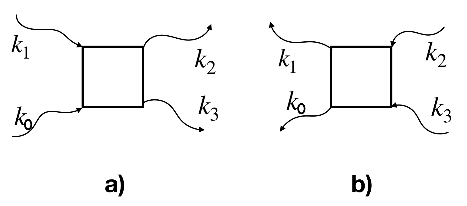
Figure 1: a) Electron-electron scattering between an electron in a state labelled by $k_{0}$, $n_{0}$ and another in a state labelled by $k_{1}$, $n_{1}$ to states labelled by $k_{2}$, $n_{2}$ and $k_{3}$, $n_{3}$. b) Time-reversed process corresponding to the same scattering.

The generalisation of Eq. (1) to other types of scatterings between different quasi-particles (both fermions and bosons) or even different number of legs (a.k.a. involved states) keeps the mathematical structure unchanged. For this reason we will show the numerical method for the time propagation in Eq. (1) only, yet it is general to any type of scattering. Let us, however, remind that calculating quasiparticle dispersions $\epsilon_{n}\left(\mathbb{k}\right)$ and the momenta-resolved amplitudes $w\left(\mathbb{k}_{0},\mathbb{k}_{1},\mathbb{k}_{2},\mathbb{k}_{3}\right)$, which are required as input in Eq. (1), are not addressed here.

Assuming all the input functions are known, the numerical treatment of Eq. (1) still presents several critical challenges. 1) The integral in Eq. (1) is high dimensional and it contains several (depending on the dimensionality of the system) Dirac deltas, one of which has a highly non trivial form. This means that the scattering term requires the execution of integrals over an extremely complex high-dimensional hyper-surface. 2) As all the populations appearing in Eq. (1) are time dependent and known only at runtime, the integral operator on the right-hand side is a quartic operator. This leads to a very prohibitive scaling of the storage and computational cost, if straightforward methods are used. 3) It is imperative to construct a numerical method that is able to conserve exactly particle number, total momentum and total energy, regardless of the achieved numerical precision. In the absence of such property, any numerical method can be exploited only for limited time propagations or under some strict conditions and approximations.

In the following sections we will address how to extend the method we developedMichael in two major ways: 1) the increase of the order of convergence, by using second degree piecewise continuous polynomial basis functions and 2) the use of a more advanced, higher order time stepping algorithm with adaptive timestep.

III Momentum space discretization

We present in this section the necessary changes to our methodMichael in order to increase the momentum space order of convergence. We restrict ourselves in this work to one dimensional materials, yet it can be generalised to higher dimensions. For the reader’s convenience we will briefly summarise the structure of the method, which is independent of the basis functions. We will then introduce the second degree basis functions used in this work. Then we will show how the construction of the scattering tensor has to be modified to account for the use of second degree polynomial basis functions, and how to construct the scattering elements.

We assume the distribution functions $f_{n}\left(t,k\right)$ and the dispersion relation $\epsilon_{n}\left(k\right)$ for a given band $n$ are defined over a certain domain, which can be a compact subset of the Brillouin zone. The method will work even when a different domain is chosen for each band, allowing computational savings as certain regions of the Brillouin zone might not be affected by the dynamics and can be efficiently disregarded.

We now focus on a single band. We split the domain into non-overlapping regions called ’elements’ which completely cover that domain. Together, the group of elements is called a mesh. For our 1D analysis the mesh consists of divisions of the line. Again every band can have a different mesh, and even if in the present work the results are presented for uniform meshes, the method can be applied to any unstructured mesh.

III.1 Projection on local basis functions

We project all the functions defined over the domain of a given band $n$ on a set of momentum basis functions $\Psi_{\begin{subarray}{c}Aa\\ n\end{subarray}}(k)$ (which again can be different for each band). We construct these basis functions to be zero everywhere except over the element identified by the index $A$, and continuous everywhere except at the edges of the element $A$. More than one basis function with subindex $a$ can be constructed for each element as long as they are linearly independent. For instance, the distribution functions $f_{n}\left(t,k\right)$ and the dispersion relation $\epsilon_{n}\left(k\right)$ can be written as a linear combination of these basis functions:

$$\begin{split}f_{n}(t,k)&=\sum_{Bb}f_{\begin{subarray}{c}Bb\\ n\end{subarray}}(t)\;\Psi_{\begin{subarray}{c}Bb\\ n\end{subarray}}(k),\\ \epsilon_{n}(k)&=\sum_{Bb}\epsilon_{\begin{subarray}{c}Bb\\ n\end{subarray}}\;\Psi_{\begin{subarray}{c}Bb\\ n\end{subarray}}(k),\end{split}$$ (2)

where $f_{\begin{subarray}{c}Bb\\ n\end{subarray}}(t)$ and $\epsilon_{\begin{subarray}{c}Bb\\ n\end{subarray}}$ are the coefficients of the discretised population and dispersion. Notice that $f_{n}(t,k)$ has been so far only semi-discretized since the time variable in the coefficients $f_{\begin{subarray}{c}Bb\\ n\end{subarray}}(t)$ has not been discretized yet.

We further assume here (yet it is not necessary) that our basis functions are orthonormal:

$$\int dk\;\Psi_{\begin{subarray}{c}Aa\\ n\end{subarray}}(k)\;\Psi_{\begin{subarray}{c}Bb\\ n\end{subarray}}(k)=\delta_{AB}\;\delta_{ab}$$ (3)

where $\delta$ is the Kronecker delta. Projecting the collision integral in Eq. (1) on the chosen basis and using Eq. (2), the orthonormality of basis functions, and the fact that the basis functions are non zero only over a single element, we obtain the final expression for the semi-discretised form of collision integral as (see ref.Michael for a detailed derivation)

$$\begin{split}\sum_{Aa^{\prime}}\frac{df_{\begin{subarray}{c}Aa^{\prime}\\ n_{0}\end{subarray}}(t)}{dt}=\sum_{Aa}\sum_{Bb}\sum_{Cc}\sum_{Dd}S^{a^{\prime}abcd}_{\begin{subarray}{c}ABCD\\ n_{0}n_{1}n_{2}n_{3}\end{subarray}}\Bigg{(}&\left(1_{\begin{subarray}{c}Aa\\ n_{0}\end{subarray}}-f_{\begin{subarray}{c}Aa\\ n_{0}\end{subarray}}(t)\right)\left(1_{\begin{subarray}{c}Bb\\ n_{1}\end{subarray}}-f_{\begin{subarray}{c}Bb\\ n_{1}\end{subarray}}(t)\right)f_{\begin{subarray}{c}Cc\\ n_{2}\end{subarray}}(t)\;f_{\begin{subarray}{c}Dd\\ n_{3}\end{subarray}}(t)-\\ &f_{\begin{subarray}{c}Aa\\ n_{0}\end{subarray}}(t)\;f_{\begin{subarray}{c}Bb\\ n_{1}\end{subarray}}(t)\left(1_{\begin{subarray}{c}Cc\\ n_{2}\end{subarray}}-f_{\begin{subarray}{c}Cc\\ n_{2}\end{subarray}}(t)\right)\left(1_{\begin{subarray}{c}Dd\\ n_{3}\end{subarray}}-f_{\begin{subarray}{c}Dd\\ n_{3}\end{subarray}}(t)\right)\Bigg{)}\\ \end{split}$$ (4)

with

$$\begin{split}S^{a^{\prime}abcd}_{\begin{subarray}{c}ABCD\\ n_{0}n_{1}n_{2}n_{3}\end{subarray}}=\sum_{G}\int\displaylimits_{\begin{subarray}{c}A\\ n_{0}\end{subarray}}\int\displaylimits_{\begin{subarray}{c}B\\ n_{1}\end{subarray}}\int\displaylimits_{\begin{subarray}{c}C\\ n_{2}\end{subarray}}\int\displaylimits_{\begin{subarray}{c}D\\ n_{3}\end{subarray}}&dk_{0}\,dk_{1}\,dk_{2}\,dk_{3}\;\;\Psi_{\begin{subarray}{c}Aa^{\prime}\\ n_{0}\end{subarray}}(k_{0})\Psi_{\begin{subarray}{c}Aa\\ n_{0}\end{subarray}}(k_{0})\Psi_{\begin{subarray}{c}Bb\\ n_{1}\end{subarray}}(k_{1})\Psi_{\begin{subarray}{c}Cc\\ n_{2}\end{subarray}}(k_{2})\Psi_{\begin{subarray}{c}Dd\\ n_{3}\end{subarray}}(k_{3})\\ &w_{\begin{subarray}{c}n_{0}+n_{1}\\ \leftrightarrow\\ n_{2}+n_{3}\end{subarray}}\left(k_{0},k_{1},k_{2},k_{3}\right)\;\;\delta(k_{0}+k_{1}-k_{2}-k_{3}+G)\\ &\delta\Big{(}\sum_{\alpha}\epsilon_{\begin{subarray}{c}A\alpha\\ n_{0}\end{subarray}}\Psi_{\begin{subarray}{c}A\alpha\\ n_{0}\end{subarray}}(k_{0})+\sum_{\beta}\epsilon_{\begin{subarray}{c}B\beta\\ n_{1}\end{subarray}}\Psi_{\begin{subarray}{c}B\beta\\ n_{1}\end{subarray}}(k_{1})-\sum_{\gamma}\epsilon_{\begin{subarray}{c}C\gamma\\ n_{2}\end{subarray}}\Psi_{\begin{subarray}{c}C\gamma\\ n_{2}\end{subarray}}(k_{2})-\sum_{\delta}\epsilon_{\begin{subarray}{c}D\delta\\ n_{3}\end{subarray}}\Psi_{\begin{subarray}{c}D\delta\\ n_{3}\end{subarray}}(k_{3})\Big{)}\end{split}$$ (5)

where $1_{\begin{subarray}{c}Aa\\ n\end{subarray}}$ is the discretized representation of a function with a constant value of 1 over the domain, and the integrals are now only over a single element and not anymore over the full domain. We refer to $S^{a^{\prime}abcd}_{\begin{subarray}{c}ABCD\\ n_{0}n_{1}n_{2}n_{3}\end{subarray}}$ as the scattering tensor, since it contains all information about the scattering. Even if the numerical results shown in this work are obtained using orthonormal basis functions, we stress that the orthonormality assumption is not necessary and the method is immediately generalisable to a non-orthonormal basis set by simply adding a mass matrix to Eq. 4. We will not repeat here how to execute the summation in Eq. 4 as it is already described in Ref. Michael , and we will simply focus on the construction of the scattering integrals in Eq. 5.

III.2 Second degree polynomial basis functions

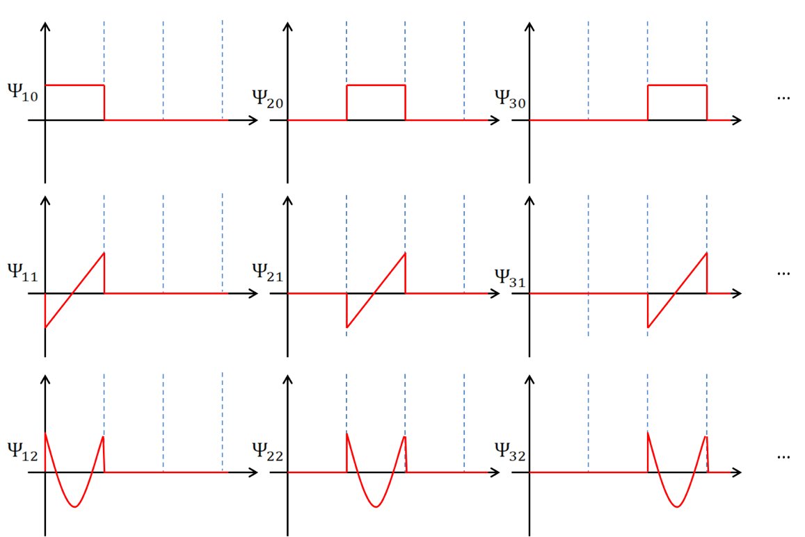
Figure 2: Example of basis functions for a given band. The band index is omitted for brevity.

To achieve a higher order of convergence compared to our previous work, we now use as basis functions second degree piecewise discontinuous polynomials with support on only one element, as shown in Fig. 2. We choose normalized Legendre polynomials of order 0,1 and 2 as basis functions for each element since they form an orthonormal set. The scaling of the number of non-zero elements of each scattering channel remains the same as in the case of linear basis functions. However, switching from first degree to second degree basis functions has three main effects. a) The time and storage cost increases in 1D and for 4-leg scatterings by a factor $(3/2)^{5}\approx 7.6$, as there are more basis functions and therefore more $(a^{\prime}abcd)$ combinations for each combination of $(ABCD)$. b) The order of convergence is however one order higher than the linear case (as it scales as $\epsilon\sim(1/N)^{(p+1)}$, where p is the maximum order of basis functions and N is the number of elements in the mesh), and, already at very low precisions, it compensates for the cost increase and outperforms the lower order approach. c) The third difference is however the most critical: the energy Dirac delta has now a quadratic function inside. This leads to a large increase in cost compared to the linear order in the pre-calculation, yet interestingly it does not affect the storage cost and the numerical cost of the time propagation.

III.3 Numerical integration of scattering tensor elements

The presence of Dirac deltas for energy and momentum conservation in Eq. (4), makes the integration domain highly discontinuous thereby making the use of a straightforward Monte Carlo integration approach impractical. However, notice that our choice of basis functions transforms the dispersion into a piecewise polynomial as shown in Eq. (5). As a result we can analytically invert both the Dirac deltas to reduce the integrand to a more manageable form. We now need to choose the variables to invert the Dirac deltas. Although all the choices are analytically equivalent, they are not so numerically. Moreover, each inversion will lead to slightly different formulas, due to sign asymmetry in Eq. (5).

Before addressing the integration, we construct a mapping of variables as $k_{1}\rightarrow x_{A};k_{2}\rightarrow x_{B};k_{3}\rightarrow-x_{C};k_{4}\rightarrow-x_{D}+G$, which makes the momentum Dirac delta completely symmetric with respect to each variable: $\delta(x_{A}+x_{B}+x_{C}+x_{D})$. By doing so, the whole integral structure becomes symmetric with respect to all the variables. Thanks to this, we can, without loss of generality, invert the Dirac deltas with respect to the first two variables. The inversion with respect to any couple of variables can be obtained simply by an appropriate simple mapping (not shown here).

In Appendix A we derive how to invert the Dirac deltas with respect to the first two variables to finally obtain an expression that has the following structure:

$$\begin{split}\Phi[&F[],l_{A},h_{A},l_{B},h_{B},l_{C},h_{C},l_{D},h_{D},\mu_{0},\mu_{A1},\mu_{A2},\mu_{B1},\mu_{B2},\mu_{C1},\mu_{C2},\mu_{D1},\mu_{D2}]=\int\displaylimits_{l_{C}}^{h_{C}}\int\displaylimits_{l_{D}}^{h_{D}}dx_{C}\;dx_{D}\\ &\Bigg{(}\frac{F[x_{A+}[x_{C},x_{D}],x_{B+}[x_{C},x_{D}],x_{C},x_{D}]}{\sqrt{\mathcal{D}[x_{C},x_{D}]}}.\Theta_{[l_{A},h_{A}]}[x_{A+}[x_{C},x_{D}]]\Theta_{[l_{B},h_{B}]}[x_{B+}[x_{C},x_{D}]]\Theta_{[0,\infty]}[\mathcal{D}[x_{C},x_{D}]]+\\ &\frac{F[x_{A-}[x_{C},x_{D}],x_{B-}[x_{C},x_{D}],x_{C},x_{D}]}{\sqrt{\mathcal{D}[x_{C},x_{D}]}}.\Theta_{[l_{A},h_{A}]}[x_{A-}[x_{C},x_{D}]]\Theta_{[l_{B},h_{B}]}[x_{B-}[x_{C},x_{D}]]\Theta_{[0,\infty]}[\mathcal{D}[x_{C},x_{D}]]\Bigg{)}\end{split}$$ (6)

where $\Theta_{[...,...]}[...]$ represents the Heaviside function between the edges (i.e. $l_{A}$ and $h_{A}$ or $l_{B}$ and $h_{B}$) of the element corresponding to the variable reduced ($x_{A}$ or $x_{B}$ in this case), $\mathcal{D}$ is the discriminant of the quadratic equation obtained when reducing the energy Dirac delta, while the basis functions and $w$ in Eq. (5) are grouped in F[…]. For the complete expressions of all the terms and a more accurate description of the integral, refer to Appendix A. Eq. (6) now does not have any internal Dirac deltas and requires an integration over a rectangular domain. In spite of the lack of Dirac deltas, the integrand has some strong discontinuities due to the presence of the Heaviside functions. In spite of the relatively low dimensionality of this integral in 1D, to be consistent with the treatment we will use in 2D and 3D materials, we use Monte Carlo to perform this integration.

The scattering tensor has some inherent symmetries, which are equivalent to particle, momentum and energy conservation. These symmetries would be automatically obeyed for an error-free calculation of the scattering tensor. However, numerical calculation introduces a finite error which in general breaks these symmetries. In Ref. Michael we symmetrised the tensor after its calculation. We highlight here that, when an apposite construction of Monte Carlo points is done (not treated here), the symmetrisation of the scattering tensor elements becomes unnecessary, and those conservations are ensured from the outset regardless of the numerical precision.

IV Time propagation algorithms

Eq. (4) is a first order, semi-discrete (since the time variable has not been discretised yet) non-linear ordinary differential equation. In principle, once the scattering tensor for a particular scattering channel is calculated, the population can be propagated in time by simply contracting the scattering tensor with the populations at that time. To complete the discretisation, we need to use a time stepping algorithm (which is a numerical algorithm for solving initial value first order ordinary differential equations). We compare in this section two different time propagation schemes: Runge-Kutta 4 (RK4) and the adaptive time stepping method, Dormand Prince 853 (DP853).

IV.1 Runge-Kutta 4

The classic RK4 is a fifth order accurate method. It is easy to implement and, more importantly, it requires only 4 function evaluations per step in timepress2007numerical . RK4 is the most commonly used general purpose time stepping algorithm given that it combines ease of implementation, sufficient stability, good computational cost, a good order of convergence, and usually performs sufficiently well on a very large class of problems.

However, RK4 scheme also presents some serious limitations. The most critical for the present problem is that the timestep is fixed and needs to be provided by the user. This has two major drawbacks. Firstly, usually one would like to control precision (or tolerance to error) of the solution. With RK4 this must be done a posteriori by controlling the timestep. Moreover this must be done directly by the user, leading to an overuse of human time and decreased efficiency. For that reason, it would be beneficial to have a method that can decide the timestep itself.

However the most critical problem is that often dynamics can evolve through different timescales, with, for instance, a first timescale with relatively high time derivatives evolving towards a slower timescale with much smaller derivatives. This is the typical behaviour of the Boltzmann scattering operator, especially when several quasiparticles and bands are involved. This means that the error at a given step in time and, more importantly, the stability condition change throughout the dynamics. The fact that the timestep is fixed in RK4, means that it must be chosen according to the strictest restrictions, even if for the greatest part of the time propagation that chosen time step ends up being unnecessarily small. As a result the actual wall time of the simulations (the real computational cost) is inflated with no benefit on the precision.

RK4 still remains a powerful method in its simplicity, and we will use it to benchmark our results. Moreover in certain situations, especially when the system does not transition between different timescales, or (not shown here) in the presence of static electric fields, RK4 can still maintain a computational advantage over more advanced methods.

IV.2 Adaptive time step Dormand Prince 853

Following the conclusions of the previous section we choose to implement an adaptive time stepping algorithm. These algorithms relieve the user from the task of setting the timestep, and, more importantly, allow for the timestep to be constantly adapted to convergence and stability requirements at each step. These algorithms usually work according to the following strategy. 1) They attempt a propagation with a given timestep $\Delta t$ (usually estimated from the previous steps). 2) They estimate the error. 3) They compare the error with the required accuracy, and if below it, they accept the step and advance the time by $\Delta t$, otherwise the solution is discarded and restart from step 1 with a new estimation of $\Delta t$.

Here we implement adaptive time stepping according to the Dormand Prince 853 method dormand1986runge which is an eight order embedded Runge Kutta method. It uses 12 function evaluation per attempted step to both calculate the numerical solution and estimate the error. For details on the implementation see Ref. DP853_Implementation .

There is one last problem to address when using adaptive time stepping algorithms. Since the algorithm constantly adapts the timestep the output is constructed at non-uniformly spaced time values. This makes plotting and comparison with experiments or other simulations difficult. For this reason, all adaptive time step algorithms allow for interpolation of the solution between steps in time with high order accuracy. To distinguish this output from the direct output of the method, it is referred to as dense output. DP853 allows for the construction of a seventh order accurate dense output, yet achieving this accuracy between the adaptive timesteps requires further 3 function evaluations per step. Let us stress that dense output only serves to provide the user with interpolated values of the solution at the user-specified regular time intervals and that it does not affect the time stepping of DP853 in any way: DP853 uses its own previous time step solution to estimate the next time step value, not the dense output.

In spite of the vastly increased complexity of the solver compared to RK4, DP853 proves to be computationally advantageous compared to RK4 in the long run.

IV.2.1 Modifications to the error estimation

The version of DP853 that we have implemented follows very closely Ref. DP853_Implementation . However we have importantly modified the error evaluation to address some specific features of the Boltzmann scattering term. Before addressing the changes we have made, we first need to summarise the way typical Dormand Prince methods estimate the error. As there are quite some technicalities involved with DP853, and it is not our intention to repeat here a full description of this method, we will instead provide a brief description of the simpler Dormand Prince 5 (DP5) and show how we modify the error estimation in that case. The interested reader can easily apply our extension to DP853.

DP methods, being embedded RK methods, can estimate the solution at different orders of accuracy. DP5 begins the estimation of the error by taking the difference between two solutions at different orders

$$\left|\Delta_{n}(k)\right|=\left|f_{n}^{[5]}(k)-f_{n}^{[4]}(k)\right|$$ (7)

where $\Delta_{n}(k)$ is the band- and momentum-resolved absolute value of the difference between the fifth-order RK estimation $f_{n}^{[5]}(k)$ and the fourth-order one $f_{n}^{[4]}(k)$. We want to compare the $k$-resolved difference with the so called scale which represents the local error that we are ready to tolerate. It is constructed by adding two terms:

$$\mbox{scale}_{n}(k)=\mbox{atol}_{n}+\left|f_{n}^{[5]}(k)\right|\;\mbox{rtol}_{n}$$ (8)

The first term $\mbox{atol}_{n}$ is the absolute tolerance (which we allow to be band-dependent) and refers to the acceptable absolute error in the population. The second term gives the acceptable error as the product of a relative tolerance $\mbox{rtol}_{n}$ and the value of the function (for which the highest order estimation is used). This allows for the error estimation to be controlled as a fraction of the actual population, unless such quantity becomes lower than the absolute tolerance, in which case the less strict requirement applies. The square of the normalised error is then estimated as

$$\left(\epsilon_{\tiny\mbox{DP}5}\right)^{2}=\frac{1}{N}\sum_{n}\left(\int\left(\frac{\left|\Delta_{n}(k)\right|}{\mbox{scale}_{n}(k)}\right)^{2}dk\Bigg{/}\int dk\right),$$ (9)

where $N$ is the number of bands, and each integral runs over each band’s domain (even if the domain is not explicitly written for shortness).

We can now introduce the first modification done to the error estimation. The relative tolerance term has the role of ensuring that the error is smaller than the information carried by the solution. Usually this information is the distance of the value of the solution from 0. However that is not necessarily always the case for fermionic populations. If the population is smaller than 0.5 then the relevant quantity is the number of electrons. However when the population is above 0.5, the system is better described by holes, and we want our precision to be compared to the number of holes i.e. ($1-f$). Therefore we want to make sure that the relative tolerance estimation works equally well for electrons and holes. We modify the scale for fermionic bands as

$$\mbox{scale}_{n}(k)=\mbox{atol}_{n}+\min\left(\left|f_{n}^{[5]}(k)\right|,\left|1-f_{n}^{[5]}(k)\right|\right)\;\mbox{rtol}_{n}$$ (10)

while no change is done for bosonic bands.

The second modification to the error estimation for DP853 is motivated by a different problem. The Boltzmann scattering term is an operator which has several fixed points. These fixed points include thermal equilibrium distributions (more fixed points exist, but it is not really relevant for this discussion). However that is true only when the populations acquire physically meaningful values: if the population somewhere is negative, or, for fermions, above 1, there is no guarantee that Eq. 1 will converge to a thermal equilibrium (yet it still might). If at any step in time the solution acquires unphysical values somewhere, the time evolution of Eq. 1 might lead to a complete divergence of the population. Notice that this would be still the legitimate time propagation of that initial condition and therefore DP has no way of recognising this behaviour by looking at the error. This means that an error, even within the acceptable tolerance, when leading to unphysical values of the solution, can cause catastrophic instabilities in the solution.

To prevent that behaviour we have to do an error estimation that does not treat all the errors of the same amplitude equally. An error that keeps the population within the window of physical values is treated in the standard way. On the other hand we artificially amplify any error that would lead the solution to acquire unphysical values. To achieve that, for each band, we add the following terms to the squared error in Eq. 9:

$$\left(\epsilon_{n}\right)^{2}=\mbox{p}_{n}\;\int\left(\frac{\Theta\left(-f_{n}^{[5]}(k)\right)}{\mbox{scale}_{n}(k)}\right)^{2}dk\Bigg{/}\int dk,$$ (11)

where $\mbox{p}_{n}$ is a penalisation factor (that we allow to be band dependent), and $\Theta$ is the unit step function. For fermionic bands we add the following further contribution to the squared error

$$\left(\epsilon_{{\tiny\mbox{ferm}},n}\right)^{2}=\mbox{p}_{n}\;\int\left(\frac{\Theta\left(f_{n}^{[5]}(k)-1\right)}{\mbox{scale}_{n}(k)}\right)^{2}dk\Bigg{/}\int dk$$ (12)

which penalises solutions with values above 1. DP, in its effort to contain the error by acting on the timestep, will then reject the step when these problematic cases arise, and reduce the timestep.

We remind that all the above expressions enter the code in their discretised versions (which we do not show here for brevity).

V Numerical results

We show numerical results obtained with the use of quadratic basis functions, and compare the performance of the two introduced time propagation schemes. It is not our intent here to address physically interesting cases, but only to show the capabilities and performance of the method on a minimal case study: a two band system. In view of applying the algorithm to the thermalisation dynamics of carbon nanotubes, we choose to describe a 1D semiconducting material. In order to highlight that the implementation can handle bands defined on different meshes, we describe an indirect bandgap semiconductor. Finally to show that the code works for arbitrary dispersions and how they can be taken from ab initio calculations, we use as dispersions those of two electronic bands of (6,5) carbon nanotubes (CNT) close to the Fermi level (see Fig. 3a) as calculated using tight-bindingmalic2013graphene . We include all possible electron-electron scattering channels obtainable with these two bands, as listed in table 1. Again it is not our purpose to describe a realistic system, so we choose all the scattering amplitudes, $w^{e-e}$, to be the same and equal to a constant 1, except for scattering channels 1, 3, and 5. For these the dependence on the momenta is chosen to be a constant 1 everywhere except in regions where the transferred momentum becomes smaller than 0.1. In that region the $w^{e-e}$ is chosen to be linear with the transferred momentum. This mimics the property of real scattering amplitude, which vanishes when the initial and final state are identical. Notice that enforcing this property is necessary as it is required to avoid a divergence of the scattering integral due to a divergence in the joint density of states. Nonetheless we stress that the choice of the dependence of the scattering matrix elements on the momenta is arbitrary and simply meant to display the capabilities of the method.

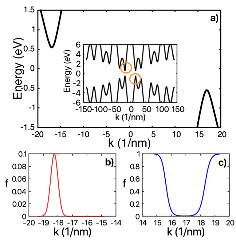
Figure 3: a) Band structure considered for the calculations done in this work. Inset: Band structure of CNT(6,5) calculated using tight binding malic2013graphene from which the dispersions used in this work have been extracted. The circles mark the part of dispersion selected for this study. b) and c) Initial out-of-equilibrium distribution of electron population in the two bands. The chemical potential $\mu$ is set to -1 eV and the temperature value is set to 1000 for band 2 (c). Band 1 has been filled with a non equilibrium distribution (b) chosen to be a Gaussian centered at k=-18.25 with a spread of 0.25 and amplitude of 0.1 eV.

Scattering Channel number	Scattering Process
1	1+1 $\Longleftrightarrow$ 1+1
2	1+1 $\Longleftrightarrow$ 1+2
3	1+2 $\Longleftrightarrow$ 1+2
4	2+2 $\Longleftrightarrow$ 2+1
5	2+2 $\Longleftrightarrow$ 2+2
6	1+1 $\Longleftrightarrow$ 2+2

Table 1: List of all scattering channels included. The numbers on the left column refer to band numbers (1 for conduction band and 2 for valence band). For instance $2+2\Longleftrightarrow 2+1$ describes a scattering channel where two electrons in band 2 scatter into band 1 and band 2.

V.1 Time propagation: Runge Kutta 4

To test the method we choose an out-of-equilibrium population as initial condition (see Fig. 3 b and c) and let the code propagate the populations in all the bands. Notice that since the scattering amplitude is in arbitrary units, the time is in arbitrary units as well. In Fig. 4 we show the evolution of the populations. The calculations have been done with 100 elements per band (for a total of 600 basis functions), and a RK4 timestep of 0.001. We observe that the initial out-of-equilibrium distribution in the bands thermalises with time. To accommodate for the added particles and energy (the initial gaussian excitation in the higher energy band) the thermalized distribution broadens in both bands as seen from Fig. 4. The shift of the peak in band 1 towards the center of the domain indicates a re-distribution of the momentum between the two bands. Notice that when umklapp scatterings are present, total momentum is not preserved, as these scatterings preserve it only up to a reciprocal lattice vector $G$. Since we constructed the Brillouin zone to be much wider than the momentum domain of the bands, umklapp scatterings (which the solver tries to construct by default) are absent. This implies that the total momentum is conserved to machine precision. We have also verified that the code conserves total particles and total energy to machine precision.

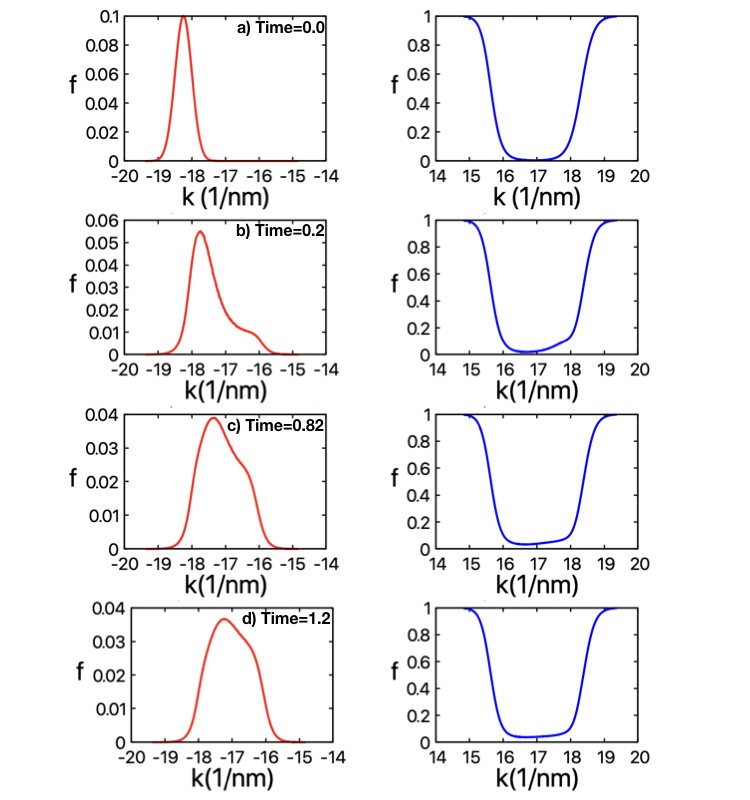
Figure 4: Time propagation of the initial electron population distribution in band 1 (left side) and band 2 (right side) with RK4 scheme. a), b), c) and d) show the different successive snap shots of the time propagation. Adaptive time stepping with DP853 shows the same thermalization profiles (not shown).

Before proceeding to the numerical evaluation of the method, as an interesting analysis tool we define a quantity that indicates the distance from equilibrium. We define the distance between two populations $f(k)$ and $g(k)$ in a given band as

$$d(f(k),g(k))=\left(\int\left(f(k)-g(k)\right)^{2}dk\right)^{1/2}$$ (13)

and denote the band-resolved distance from equilibrium $DEq_{n}$ as the distance between the population $f_{n}(k,t)$ of that band $n$ at any given time $t$

$$DEq_{n}=d(f_{n}(k,t),f_{eq,n}(k))$$ (14)

and the equilibrium condition $f_{eq,n}(k)=\lim_{t\to\infty}f_{n}(k,t)$. The distance from equilibrium for the conduction band (as shown in Fig. 5) is not a simple exponential decay.

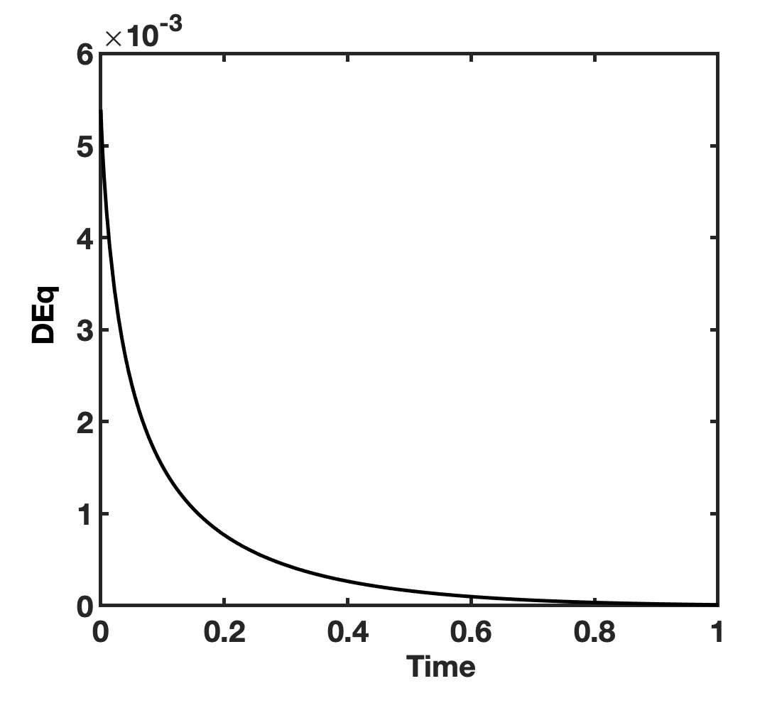
Figure 5: Distance from equilibrium (as defined in Eq. 14) for the time propagation of the excitation shown in Fig. 3 using RK4 scheme. The band index is omitted for brevity.

We test here the dependence of the precision of RK4 on the timestep. To construct the error, we need the exact solution. As that is not accessible, we perform a DP853 calculation with a very small absolute and relative tolerance (1e-16 for both the bands), and take this solution as a good estimation of the exact solution. We then perform a series of RK4 calculations with increasingly larger timesteps and calculate the distance between the predicted population at time $t=0.4$ with our nearly exact solution at $t=0.4$. In Fig. 6 we show the influence of the time step on the error.

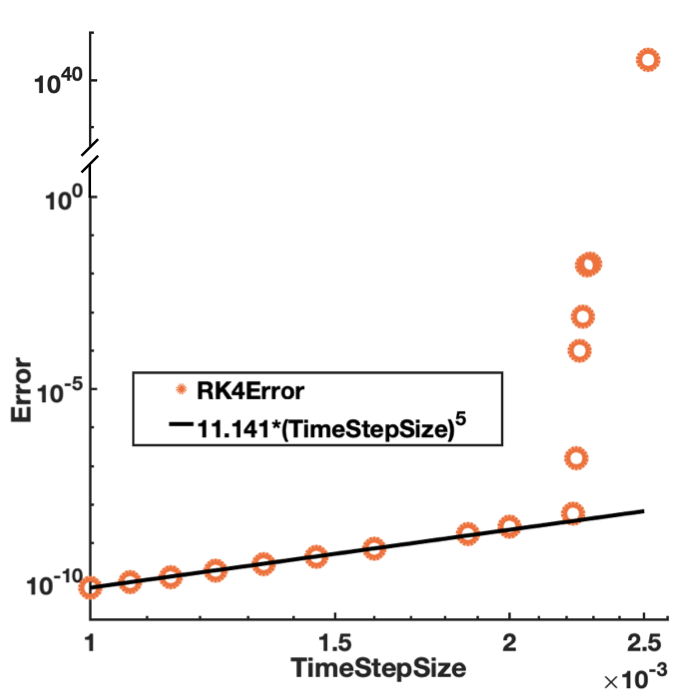
Figure 6: Variation of Error with the timestep size for RK4. For smaller time steps the error varies with the fifth power of the time step size.

Figure 7: Effect of instability on the population. Right) Stable solution at time $t=0.4$. Left) Solution at time $t=0.4$ when the RK4 time propagation becomes unstable.

We observe that with increasing timestep the error increases as $\delta t^{5}$ as expected. We can also observe the appearance of instability, when the timestep increases above a certain threshold. In Fig.7 we show the population for a timestep of $0.0022$ where instability in the solution is just appearing, and the one for a timestep of $0.0025$ where instead the solution has completely diverged.

V.2 Time propagation: Dormand Prince 853

The observation that the system’s thermalisation evolves through different timescales (Fig. 5), hints that a full propagation with a single timestep is inefficient. Early times require small timesteps, while later times could permit the use of longer ones. Even if that can be done by the user manually in RK4 by stopping the simulation, changing the timestep and then continuing, adaptive time stepping methods like DP853 are preferable in these cases, as they perform that task automatically at each timestep and optimise the choices.

The analysis of the convergence order of DP853 itself is less straightforward compared to RK4, as there is no fixed timestep. Moreover the computational cost is not directly linked to the number of performed steps, since a fraction of the steps are rejected. We first show in fig. 8 the behaviour of the error in the solution after a time, t=0.4 in dependence of the accepted and total (meaning accepted plus rejected) steps in time. Both values are indirectly controlled by setting the tolerances mentioned in the previous section. We observe that the error scales with the ninth power of the total timesteps at lower tolerances or higher number of time steps. It can be noted from Fig. 8 that the number of rejected timesteps (i.e. the difference between the number of total timesteps and the number of successful timesteps) tends to remain relatively constant over the full range of required tolerances (please notice the logarithmic scale). We observe that most of the rejections happen at the beginning of the calculation. DP853 uses the error obtained using the initial guess for timestep (which we provide as large) to make a better guess. This takes a few iterations before DP853 obtains a value of the time step that gives an acceptable error. From that point on DP853 is very efficient in predicting a time step for the next iteration and rarely rejects future steps.

Figure 8: Variation of Error for DP853 with the number of steps. At higher number of steps, i.e. higher tolerances, the error varies with the ninth power of the number of the time steps.

We can now compare DP853 and RK4. The number of total steps taken does not provide a fair comparison, since the computational cost at each step is very different for the two methods. We therefore compare in Fig. 9 the wall time (actual time that it takes for the time propagation) at parity of error. As seen from Fig. 9 DP853 vastly outperforms RK4. This is partially due to the much higher convergence order. However notice that RK4 diverges if the numerical effort is too low. This is due to the fact that while DP853 adapts its step and can take shorter time steps at early times when the dynamics is fast and then save computational resources later, RK4 does not have this flexibility and its overall stability is linked to the worst case timescale. For a required error precision of 1e-4, which can be considered acceptable, the cost of RK4 is approximately 45 times the cost of DP853.

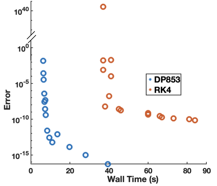
Figure 9: Comparison of the computational cost of DP853 and RK4.

However Fig. 9 does not account for one of the greatest advantages of DP853 over RK4. In RK4 the user needs to test timestep sizes and observe the solution to evaluate its quality. This approach has both a numerical and, even more importantly, a human cost, not included in the comparison in Fig. 9. This makes the real wall time for RK4 much higher than the one for DP853, in almost all the cases.

V.3 Dormand Prince 853: Dense output

It is worth however highlighting one problem we encountered when using DP853. The method computes the solution with eight-order accuracy at irregular time intervals. However this output, due to this characteristic, is seldom useful. The order of convergence of the dense output is one order lower. That means that while DP853 controls the error of the eight-order embedded Runge Kutta method by comparing it to the tolerances assigned by the user, the useful output (the dense one) has a (sometimes importantly) higher error. This difference in the orders of convergence can lead to very evident errors. In Fig. 10 we show one case where the eight-order solution at the adaptive steps has an extremely low error, while the seventh-order one at the dense time mesh shows evident errors. One might see this from a different point of view: while the solution produced on the adapted times has a high precision, the lower order interpolation, used to produce the solution on the dense mesh has a lower precision. This is an issue the user should be aware of, yet it is easily solvable by running another simulation with smaller tolerances with the effect of reducing the error in both orders. This is rarely a problem, since, given the high order of convergence, usually an even rather large decrease in the required tolerance leads to a very small increase in computational time.

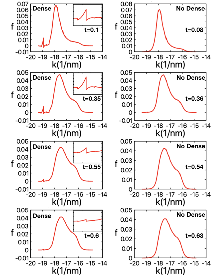
Figure 10: Comparison between the eight-order solution (on the adaptive time steps) and the seventh-order solution (on the closest point of the dense mesh) for DP853. Inset: Zoomed in discontinuity of the solution. To magnify the effect of numerical accuracy we choose a lower mesh resolution of n=20 elements and set the tolerance values to 1e-2 for this case.

VI Conclusions

Concluding, we have extended in two major ways the method we developed in Ref. Michael for the solution (without any approximation) of the time-dependent Boltzmann scattering integral for strongly-out-of-equilibrium scenarios and for realistic band structures and matrix elements. 1) We have extended the treatment to higher order basis functions, gaining one order of convergence in momentum space. 2) We have implemented a powerful adaptive time step scheme and shown how to modify it to address the issues typical of this equation. We have shown how these improvements work and allow for flexible and multipurpose calculations of the ultrafast time propagation of femtosecond excitations in solids.

Appendix Appendix A Scattering elements with second order basis functions

We here address the task of computing the scattering elements in Eq. 5. As already mentioned we first perform the mapping of variables as: $k_{1}\rightarrow x_{A};k_{2}\rightarrow x_{B};k_{3}\rightarrow-x_{C};k_{4}\rightarrow-x_{D}+G$, to express the integral in a form that is symmetric with respect to the variables. It can be shown that the integral assumes the following general form:

$$\begin{split}\Phi&[F(),l_{A},h_{A},l_{B},h_{B},l_{C},h_{C},l_{D},h_{D},\mu_{0},\mu_{A1},\mu_{A2},\mu_{B1},\mu_{B2},\mu_{C1},\mu_{C2},\mu_{D1},\mu_{D2}]\\ &=\int_{l_{A}}^{h_{A}}\int_{l_{B}}^{h_{B}}\int_{l_{C}}^{h_{C}}\int_{l_{D}}^{h_{D}}dx_{A}dx_{B}dx_{C}dx_{D}\;F\left(x_{A},x_{B},x_{C},x_{D}\right)\;\delta(x_{A}+x_{B}+x_{C}+x_{D})\\ &\delta(\mu_{0}+\mu_{A1}x_{A}+\mu_{A2}x_{A}^{2}+\mu_{B1}x_{B}+\mu_{B2}x_{B}^{2}+\mu_{C1}x_{C}+\mu_{C2}x_{C}^{2}+\mu_{D1}x_{D}+\mu_{D2}x_{D}^{2})\end{split}$$ (A.15)

where the function $F()$ incorporates the basis functions and the scattering matrix element, while the coefficients, $\mu_{0}$, $\mu_{A1}$ etc. result from expressing the coefficients of the dispersions and the basis functions, everything after the appropriate variable transformation.

Without loss of generality, we now choose the variables $x_{A}$ and $x_{B}$ to analytically invert the Dirac deltas. By reducing the first Dirac delta, we can write the first variable as

$$x_{A}[x_{B},x_{C},x_{D}]=-x_{B}-x_{C}-x_{D}.$$ (A.16)

We can now substitute this in the energy Dirac delta and collect all the terms with the same power of $x_{B}$ to find:

$$\delta\left(energy\right)=\delta\left(\alpha x_{B}^{2}+\beta[x_{C},x_{D}]x_{B}+\gamma[x_{C},x_{D}]\right)$$ (A.17)

where

$$\alpha=\mu_{A2}+\mu_{B2}$$ (A.18)

$$\beta[x_{C},x_{D}]=\mu_{B1}-\mu_{A1}+2\mu_{A2}(x_{C}+x_{D})$$ (A.19)

$$\gamma[x_{C},x_{D}]=\mu_{0}+(\mu_{C1}-\mu_{A1})x_{C}+$$ (A.20)

$$\;\;\;\;\;\;\;\;\;+(\mu_{A2}+\mu_{C2})x_{C}^{2}++(\mu_{D1}-\mu_{A1})x_{D}+$$

$$\;\;\;\;\;\;\;\;\;+(\mu_{A2}+\mu_{D2})x_{D}^{2}+2\mu_{A2}x_{C}x_{D}$$

The quadratic form inside the Dirac delta in Eq. A.17, possesses two roots with respect to the variable $x_{B}$. Notice that these roots $x_{B+}[x_{C},x_{D}]$ and $x_{B-}[x_{C},x_{D}]$ are dependent on the last two variables and are real only where the discriminant

$$D[x_{C},x_{D}]=\beta^{2}[x_{C},x_{D}]-4\alpha[x_{C},x_{D}]\gamma[x_{C},x_{D}]$$ (A.21)

is positive. We can now rewrite Eq. A.15 as

$$\begin{split}\Phi[...]=\int_{l_{C}}^{h_{C}}\int_{l_{D}}^{h_{D}}dx_{C}dx_{D}\Bigg{(}&\frac{F[x_{A+}[x_{C},x_{D}],x_{B+}[x_{C},x_{D}],x_{C},x_{D}]}{\sqrt{D[x_{C},x_{D}]}}\cdot\\ &\cdot\Theta_{[l_{A},h_{A}]}[x_{A+}[x_{C},x_{D}]]\;\;\Theta_{[l_{B},h_{B}]}[x_{B+}[x_{C},x_{D}]]\;\;\Theta_{[0,\infty]}[D[x_{C},x_{D}]]\\ &+\frac{F[x_{A-}[x_{C},x_{D}],x_{B-}[x_{C},x_{D}],x_{C},x_{D}]}{\sqrt{D[x_{C},x_{D}]}}\cdot\\ &\cdot\Theta_{[l_{A},h_{A}]}[x_{A-}[x_{C},x_{D}]]\;\;\Theta_{[l_{B},h_{B}]}[x_{B-}[x_{C},x_{D}]]\;\;\Theta_{[0,\infty]}[D[x_{C},x_{D}]]\Bigg{)},\end{split}$$ (A.22)

where the first (second) addend in the brackets comes to the first (second) root. The $\Theta[...]$ represents the Heaviside function. The first two Heaviside functions derive from the limits of the integration in the first two variables. The third $\Theta[...]$ function, ensures that the integral is not performed over complex solutions.

The expression in Eq. A.22 is now a lower dimensional integral finally over a function and not anymore a distribution (in the sense of a generalised function). However this is not a smooth function due to the presence of the Heaviside functions. We are now free to perform this integral by any numerical technique. For consistence to the technique that we will use in higher dimensions, we performed this integral with Monte Carlo.

References

- [1] Michael Wais, Karsten Held, and Marco Battiato. Deterministic solver for the time-dependent far-from-equilibrium quantum boltzmann equation. arXiv preprint arXiv:2004.02683, 2020.
- [2] J. G. Fujimoto, J. M. Liu, E. P. Ippen, and N. Bloembergen. Femtosecond laser interaction with metallic tungsten and nonequilibrium electron and lattice temperatures. Phys. Rev. Lett., 53:1837–1840, Nov 1984.
- [3] H. E. Elsayed-Ali, T. B. Norris, M. A. Pessot, and G. A. Mourou. Time-resolved observation of electron-phonon relaxation in copper. Phys. Rev. Lett., 58:1212–1215, Mar 1987.
- [4] R. W. Schoenlein, W. Z. Lin, J. G. Fujimoto, and G. L. Eesley. Femtosecond studies of nonequilibrium electronic processes in metals. Phys. Rev. Lett., 58:1680–1683, Apr 1987.
- [5] S. D. Brorson, A. Kazeroonian, J. S. Moodera, D. W. Face, T. K. Cheng, E. P. Ippen, M. S. Dresselhaus, and G. Dresselhaus. Femtosecond room-temperature measurement of the electron-phonon coupling constant in metallic superconductors. Phys. Rev. Lett., 64:2172–2175, Apr 1990.
- [6] W. S. Fann, R. Storz, H. W. K. Tom, and J. Bokor. Electron thermalization in gold. Phys. Rev. B, 46:13592–13595, Nov 1992.
- [7] T. Hertel, E. Knoesel, M. Wolf, and G. Ertl. Ultrafast electron dynamics at cu(111): Response of an electron gas to optical excitation. Phys. Rev. Lett., 76:535–538, Jan 1996.
- [8] N. Del Fatti, C. Voisin, M. Achermann, S. Tzortzakis, D. Christofilos, and F. Vallée. Nonequilibrium electron dynamics in noble metals. Phys. Rev. B, 61:16956–16966, Jun 2000.
- [9] C. Stamm, T. Kachel, N. Pontius, R. Mitzner, T. Quast, K. Holldack, S. Khan, C. Lupulescu, E. F. Aziz, M. Wietstruk, H. A. Dürr, and W. Eberhardt. Femtosecond modification of electron localization and transfer of angular momentum in nickel. Nature Materials, 6:740–743, 2007.
- [10] E. Beaurepaire, J.-C. Merle, A. Daunois, and J.-Y. Bigot. Ultrafast spin dynamics in ferromagnetic nickel. Phys. Rev. Lett., 76:4250–4253, May 1996.
- [11] Yasuhiko Terada, Shoji Yoshida, Atsushi Okubo, Ken Kanazawa, Maojie Xu, Osamu Takeuchi, and Hidemi Shigekawa. Optical doping active control of metal insulator transition in nanowire. Nano Lett., 8(11):3577–3581, 2008.
- [12] A. Crepaldi, B. Ressel, F. Cilento, M. Zacchigna, C. Grazioli, H. Berger, Ph. Bugnon, K. Kern, M. Grioni, and F. Parmigiani. Ultrafast photodoping and effective fermi-dirac distribution of the dirac particles in bi2se3. Phys. Rev. B, 86:205133, Nov 2012.
- [13] Guillermo Garcia, Raffaella Buonsanti, Evan L. Runnerstrom, Rueben J. Mendelsberg, Anna Llordes, Andre Anders, Thomas J. Richardson, and Delia J. Milliron. Dynamically modulating the surface plasmon resonance of dopedsemiconductor nanocrystals. Nano Lett., 11(10):4415–4420, 2011.
- [14] C. Cacho, A. Crepaldi, M. Battiato, J. Braun, F. Cilento, M. Zacchigna, M. C. Richter, O. Heckmann, E. Springate, Y. Liu, S. S. Dhesi, H. Berger, Ph. Bugnon, K. Held, M. Grioni, H. Ebert, K. Hricovini, J. Minár, and F. Parmigiani. Momentum-resolved spin dynamics of bulk and surface excited states in the topological insulator . Phys. Rev. Lett., 114:097401, Mar 2015.
- [15] M. Battiato, J. Minár, W. Wang, W. Ndiaye, M. C. Richter, O. Heckmann, J.-M. Mariot, F. Parmigiani, K. Hricovini, and C. Cacho. Distinctive picosecond spin polarization dynamics in bulk half metals. Phys. Rev. Lett., 121:077205, Aug 2018.
- [16] Liang Cheng, Xinbo Wang, Weifeng Yang, Jianwei Chai, Ming Yang, Mengji Chen, Yang Wu, Xiaoxuan Chen, Dongzhi Chi, Kuan Eng Johnson Goh, Jian-Xin Zhu, Handong Sun, Shijie Wang, Justin C. W. Song, Marco Battiato, Hyunsoo Yang, and Elbert E. M. Chia. Far out-of-equilibrium spin populations trigger giant spin injection into atomically thin mos2. Nature Physics, 15(4):347–351, 2019.
- [17] A. I. Frenkel, D. M. Pease, J. I. Budnick, P. Metcalf, E. A. Stern, P. Shanthakumar, and T. Huang. Strain-induced bond buckling and its role in insulating properties of cr-doped v2o3. Phys. Rev. Lett., 97:195502, Nov 2006.
- [18] Markus Lindemann, Gaofeng Xu, Tobias Pusch, Rainer Michalzik, Martin R. Hofmann, Igor žutić, and Nils C. Gerhardt. Ultrafast spin-lasers. Nature, 568:212, 2019.
- [19] G Malinowski, F Dalla Longa, JHH Rietjens, PV Paluskar, R Huijink, HJM Swagten, and B Koopmans. Control of speed and efficiency of ultrafast demagnetization by direct transfer of spin angular momentum. Nature Physics, 4(11):855–858, 2008.
- [20] Marco Battiato, Karel Carva, and Peter M Oppeneer. Superdiffusive spin transport as a mechanism of ultrafast demagnetization. Physical review letters, 105(2):027203, 2010.
- [21] Dennis Rudolf, La-O-Vorakiat Chan, Marco Battiato, Roman Adam, Justin M Shaw, Emrah Turgut, Pablo Maldonado, Stefan Mathias, Patrik Grychtol, Hans T Nembach, Thomas J Silva, Martin Aeschlimann, Henry C Kapteyn, Margaret M Murnane, Claus M Schneider, and Peter M Oppeneer. Ultrafast magnetization enhancement in metallic multilayers driven by superdiffusive spin current. Nature communications, 3(1):1–6, 2012.
- [22] Tobias Kampfrath, Marco Battiato, Pablo Maldonado, G Eilers, J Nötzold, Sebastian Mährlein, V Zbarsky, F Freimuth, Y Mokrousov, S Blügel, M Wolf, I Radu, Peter M Oppeneer, and M Münzenberg. Terahertz spin current pulses controlled by magnetic heterostructures. Nature nanotechnology, 8(4):256–260, 2013.
- [23] Andrea Eschenlohr, Marco Battiato, Pablo Maldonado, N Pontius, T Kachel, K Holldack, R Mitzner, Alexander Föhlisch, Peter M Oppeneer, and C Stamm. Ultrafast spin transport as key to femtosecond demagnetization. Nature materials, 12(4):332–336, 2013.
- [24] M Battiato and K Held. Ultrafast and gigantic spin injection in semiconductors. Physical Review Letters, 116(19):196601, 2016.
- [25] F. Freyse, M. Battiato, L. V. Yashina, and J. Sánchez-Barriga. Impact of ultrafast transport on the high-energy states of a photoexcited topological insulator. Phys. Rev. B, 98:115132, Sep 2018.
- [26] Filchito Renee G. Bagsican, Michael Wais, Natsumi Komatsu, Weilu Gao, Lincoln W. Weber, Kazunori Serita, Hironaru Murakami, Karsten Held, Frank A. Hegmann, Masayoshi Tonouchi, Junichiro Kono, Iwao Kawayama, and Marco Battiato. Terahertz excitonics in carbon nanotubes: Exciton autoionization and multiplication. Nano Letters, 20(5):3098–3105, 2020. PMID: 32227963.
- [27] Ludwig Boltzmann. Weitere studien über das wärmegleichgewicht unter gasmolekülen. Sitzungsberichte der Kaiserlichen Akademie der Wissenschaften., 66:275, 1872.
- [28] Simon M. Sze and Kwok K. Ng. Physics of Semiconductor Devices. Wiley-Interscience, 1969.
- [29] Carlo Cercignani. The boltzmann equation. In The Boltzmann equation and its applications, pages 40–103. Springer, 1988.
- [30] N. Ben Abdallah and P. Degond. On a hierarchy of macroscopic models for semiconductors. Journal of Mathematical Physics, 37(7):3306–3333, 1996.
- [31] Gerald D. Mahan. Many-Particle Physics. Kluwer Academic/Plenum Publishers, New York, 2000.
- [32] Isabelle Choquet, Pierre Degond, and Christian Schmeiser. Energy-transport models for charge carriers involving impact ionization in semiconductors. Transport Theory and Statistical Physics, 32, 05 2000.
- [33] B. Rethfeld, A. Kaiser, M. Vicanek, and G. Simon. Ultrafast dynamics of nonequilibrium electrons in metals under femtosecond laser irradiation. Phys. Rev. B, 65:214303, May 2002.
- [34] Armando Majorana, Orazio Muscato, and C. Milazzo. Charge transport in 1d silicon devices via monte carlo simulation and boltzmann-poisson solver. COMPEL: The International Journal for Computation and Mathematics in Electrical and Electronic Engineering, 23:410–425, 06 2004.
- [35] María Cáceres, J. Carrillo, and Armando Majorana. Deterministic simulation of the boltzmann–poisson system in gaas-based semiconductors. SIAM J. Scientific Computing, 27:1981–2009, 01 2006.
- [36] D. W. Snoke. The quantum boltzmann equation in semiconductor physics. Annalen der Physik, 523(1-2):87–100, 2011.
- [37] Shuntaro Tani, Fran çois Blanchard, and Koichiro Tanaka. Ultrafast carrier dynamics in graphene under a high electric field. Phys. Rev. Lett., 109:166603, Oct 2012.
- [38] Vatsal A. Jhalani, Jin-Jian Zhou, and Marco Bernardi. Ultrafast hot carrier dynamics in gan and its impact on the efficiency droop. Nano Lett., 17(8):5012–5019, 2017.
- [39] Michael Wais, Martin Eckstein, Roland Fischer, Philipp Werner, Marco Battiato, and Karsten Held. Quantum boltzmann equation for strongly correlated systems: Comparison to dynamical mean field theory. Physical Review B, 98(13):134312, 2018.
- [40] Vatsal A Jhalani, Jin-Jian Zhou, and Marco Bernardi. Ultrafast hot carrier dynamics in gan and its impact on the efficiency droop. Nano Letters, 17(8):5012–5019, 2017.
- [41] Wu Li, Jesús Carrete, Nebil A Katcho, and Natalio Mingo. Shengbte: A solver of the boltzmann transport equation for phonons. Computer Physics Communications, 185(6):1747–1758, 2014.
- [42] L Lindsay, Wu Li, Jesús Carrete, Natalio Mingo, DA Broido, and TL Reinecke. Phonon thermal transport in strained and unstrained graphene from first principles. Physical Review B, 89(15):155426, 2014.
- [43] Gianpiero Colonna and Antonio D’Angola. Plasma Modeling; Methods and Applications. 2016.
- [44] Cédric Villani. A review of mathematical topics in collisional kinetic theory. Handbook of mathematical fluid dynamics, 1(71-305):3–8, 2002.
- [45] Gilberto M Kremer. An introduction to the Boltzmann equation and transport processes in gases. Springer Science & Business Media, 2010.
- [46] Laure Saint-Raymond. Hydrodynamic limits of the Boltzmann equation. Number 1971. Springer Science & Business Media, 2009.
- [47] VE Colussi, Cameron JE Straatsma, Dana Z Anderson, and MJ Holland. Undamped nonequilibrium dynamics of a nondegenerate bose gas in a 3d isotropic trap. New Journal of Physics, 17(10):103029, 2015.
- [48] David W Snoke. The quantum boltzmann equation in semiconductor physics. Annalen der Physik, 523(1-2):87–100, 2011.
- [49] Zahra Shomali, Behrad Pedar, Jafar Ghazanfarian, and Abbas Abbassi. Monte-carlo parallel simulation of phonon transport for 3d silicon nano-devices. International Journal of Thermal Sciences, 114:139–154, 2017.
- [50] Ao Xu, Wei Shyy, and Tianshou Zhao. Lattice boltzmann modeling of transport phenomena in fuel cells and flow batteries. Acta Mechanica Sinica, 33(3):555–574, 2017.
- [51] WL Morgan and BM Penetrante. Elendif: A time-dependent boltzmann solver for partially ionized plasmas. Computer Physics Communications, 58(1-2):127–152, 1990.
- [52] Aydin Nabovati, Daniel P Sellan, and Cristina H Amon. On the lattice boltzmann method for phonon transport. Journal of Computational Physics, 230(15):5864–5876, 2011.
- [53] Daniel P Sellan, JE Turney, Alan JH McGaughey, and Cristina H Amon. Cross-plane phonon transport in thin films. Journal of applied physics, 108(11):113524, 2010.
- [54] Sina Hamian, Toru Yamada, Mohammad Faghri, and Keunhan Park. Finite element analysis of transient ballistic–diffusive phonon heat transport in two-dimensional domains. International Journal of Heat and Mass Transfer, 80:781–788, 2015.
- [55] Vittorio Romano, Armando Majorana, and Marco Coco. Dsmc method consistent with the pauli exclusion principle and comparison with deterministic solutions for charge transport in graphene. Journal of Computational Physics, 302:267–284, 2015.
- [56] Ross E Heath, Irene M Gamba, Philip J Morrison, and Christian Michler. A discontinuous galerkin method for the vlasov–poisson system. Journal of Computational Physics, 231(4):1140–1174, 2012.
- [57] Bernardo Cockburn and Chi-Wang Shu. Runge–kutta discontinuous galerkin methods for convection-dominated problems. Journal of scientific computing, 16(3):173–261, 2001.
- [58] LH Li. An analytic solution of the boltzmann equation in the presence of self-generated magnetic fields in astrophysical plasmas. Physics Letters A, 246(5):436–440, 1998.
- [59] Isabelle Choquet, Pierre Degond, and Christian Schmeiser. Energy-transport models for charge carriers involving impact ionization in semiconductors. 2003.
- [60] A Majorana, O Muscato, and C Milazzo. Charge transport in 1d silicon devices via monte carlo simulation and boltzmann-poisson solver. COMPEL-The international journal for computation and mathematics in electrical and electronic engineering, 2004.
- [61] Satyvir Singh and Marco Battiato. Effect of strong electric fields on material responses: The bloch oscillation resonance in high field conductivities. Materials, 13:1070, 2020.
- [62] Satyvir Singh and Marco Battiato. Strongly out-of-equilibrium simulations for electron boltzmann transport equation using explicit modal discontinuous galerkin method. Int. J. Appl. Comput.l Math., 6:133, 2020.
- [63] Francis VanGessel, Jie Peng, and Peter W Chung. A review of computational phononics: the bulk, interfaces, and surfaces. Journal of materials science, 53(8):5641–5683, 2018.
- [64] Aleksandr Chernatynskiy and Simon R Phillpot. Evaluation of computational techniques for solving the boltzmann transport equation for lattice thermal conductivity calculations. Physical Review B, 82(13):134301, 2010.
- [65] David A Broido, Michael Malorny, Gerd Birner, Natalio Mingo, and DA Stewart. Intrinsic lattice thermal conductivity of semiconductors from first principles. Applied Physics Letters, 91(23):231922, 2007.
- [66] Lei Wu, Craig White, Thomas J Scanlon, Jason M Reese, and Yonghao Zhang. Deterministic numerical solutions of the boltzmann equation using the fast spectral method. Journal of Computational Physics, 250:27–52, 2013.
- [67] Graeme A Bird and JM Brady. Molecular gas dynamics and the direct simulation of gas flows, volume 5. Clarendon press Oxford, 1994.
- [68] Thomas MM Homolle and Nicolas G Hadjiconstantinou. A low-variance deviational simulation monte carlo for the boltzmann equation. Journal of Computational Physics, 226(2):2341–2358, 2007.
- [69] FG Tcheremissine. Solution to the boltzmann kinetic equation for high-speed flows. Computational mathematics and mathematical physics, 46(2):315–329, 2006.
- [70] Ilgis Ibragimov and Sergej Rjasanow. Numerical solution of the boltzmann equation on the uniform grid. Computing, 69(2):163–186, 2002.
- [71] Irene M Gamba and Sri Harsha Tharkabhushanam. Spectral-lagrangian methods for collisional models of non-equilibrium statistical states. Journal of Computational Physics, 228(6):2012–2036, 2009.
- [72] Lorenzo Pareschi and Giovanni Russo. Numerical solution of the boltzmann equation i: Spectrally accurate approximation of the collision operator. SIAM journal on numerical analysis, 37(4):1217–1245, 2000.
- [73] Clément Mouhot and Lorenzo Pareschi. Fast algorithms for computing the boltzmann collision operator. Mathematics of computation, 75(256):1833–1852, 2006.
- [74] Shuntaro Tani, François Blanchard, and Koichiro Tanaka. Ultrafast carrier dynamics in graphene under a high electric field. Physical review letters, 109(16):166603, 2012.
- [75] Pablo Maldonado, Karel Carva, Martina Flammer, and Peter M Oppeneer. Theory of out-of-equilibrium ultrafast relaxation dynamics in metals. Physical Review B, 96(17):174439, 2017.
- [76] John M Ziman. Electrons and phonons: the theory of transport phenomena in solids. Oxford university press, 2001.
- [77] Massimo V Fischetti and Steven E Laux. Monte carlo analysis of electron transport in small semiconductor devices including band-structure and space-charge effects. Physical Review B, 38(14):9721, 1988.
- [78] David W Snoke. Solid state physics: Essential concepts. Cambridge University Press, 2020.
- [79] William H Press, Saul A Teukolsky, William T Vetterling, and Brian P Flannery. Numerical recipes 3rd edition: The art of scientific computing. Cambridge university press, 2007.
- [80] JR Dormand and PJ Prince. Runge-kutta triples. Computers & Mathematics with Applications, 12(9):1007–1017, 1986.
- [81] Ernst Hairer, Syvert P Nørsett, and Gerhard Wanner. Solving ordinary differential equations I. Nonstiff problems, volume 8 of. Springer Series in Computational Mathematics, 1993.
- [82] Ermin Malic and Andreas Knorr. Graphene and carbon nanotubes: Ultrafast Relaxation Dynamics and Optics. Wiley-VCH, 2013.