Lepton sector in modular $A_{4}$ and gauged $U(1)_{R}$ symmetry

Abstract

We propose a lepton model under modular $A_{4}$ and gauged $U(1)_{R}$ symmetries, in which the neutrino masses are induced at one-loop level. Thanks to the modular $A_{4}$ symmetry, we have several predictions on the lepton sector, especially, on fixed points of $\tau=i,\omega\equiv e^{2\pi i/3},i\times\infty$ each of which has remnant symmetry; $Z_{2}$ for $\tau=i$ and $Z_{3}$ for $\tau=\omega,i\infty$. These points are favored by a string theory and phenomenologically interesting.

I Introduction

Right-handed gauged symmetry $U(1)_{R}$ is one of the promising candidates for physics beyond the standard model. It naturally accommodates the three right-handed fermions in order to cancel chiral anomalies, and also it and the other similar models such as gauged $U(1)_{B-L}$ symmetry can be discriminated by measuring, e.g., forward-backward asymmetry via each of the extra gauge bosons at International Linear Collider Baer:2013cma .

Recently, attractive flavor symmetries are also proposed by papers Feruglio:2017spp ; deAdelhartToorop:2011re , in which they applied modular motivated non-Abelian discrete flavor symmetries to quark and lepton sectors. One remarkable advantage is that any dimensionless couplings can also be transformed as non-trivial representations under those symmetries. Therefore, we do not need so many scalars to find a predictive mass matrix. Along this line of the idea, a vast literature has recently arisen in references, e.g., $A_{4}$ Feruglio:2017spp ; Criado:2018thu ; Kobayashi:2018scp ; Okada:2018yrn ; Nomura:2019jxj ; Okada:2019uoy ; deAnda:2018ecu ; Novichkov:2018yse ; Nomura:2019yft ; Okada:2019mjf ; Ding:2019zxk ; Nomura:2019lnr ; Kobayashi:2019xvz ; Asaka:2019vev ; Zhang:2019ngf ; Gui-JunDing:2019wap ; Kobayashi:2019gtp ; Nomura:2019xsb ; Wang:2019xbo ; Okada:2020dmb ; Okada:2020rjb ; Behera:2020lpd ; Behera:2020sfe ; Nomura:2020opk ; Nomura:2020cog ; Asaka:2020tmo ; Okada:2020ukr , $S_{3}$ Kobayashi:2018vbk ; Kobayashi:2018wkl ; Kobayashi:2019rzp ; Okada:2019xqk ; Mishra:2020gxg , $S_{4}$ Penedo:2018nmg ; Novichkov:2018ovf ; Kobayashi:2019mna ; King:2019vhv ; Okada:2019lzv ; Criado:2019tzk ; Wang:2019ovr , $A_{5}$ Novichkov:2018nkm ; Ding:2019xna ; Criado:2019tzk , larger groups Baur:2019kwi , multiple modular symmetries deMedeirosVarzielas:2019cyj , and double covering of $A_{4}$ Liu:2019khw ; Chen:2020udk , $S_{4}$ Novichkov:2020eep ; Liu:2020akv , and the other types of groups Kikuchi:2020nxn in which masses, mixing, and CP phases for quark and/or lepton are predicted.  Furthermore, a systematic approach to understand the origin of CP transformations has been discussed in Ref. Baur:2019iai , and CP violation in models with modular symmetry is discussed in Ref. Kobayashi:2019uyt ; Novichkov:2019sqv , and a possible correction from Kähler potential is discussed in Ref. Chen:2019ewa . Systematic analysis of the fixed points(stabilizers) has been discussed in ref. deMedeirosVarzielas:2020kji .

In this paper, we combine these features of the gauged $U(1)_{R}$ based on our recent paper Nagao:2020azf and a modular $A_{4}$ symmetry, in which we construct lepton Yukawa Lagrangian while the neutrino mass is generated by non-trivial Yukawa couplings at one-loop level. Due to the $A_{4}$ nature, the charged-lepton mass matrix is diagonal at the flavor eigenstate. And we find specific Yukawa and mass matrices that lead to several predictions when we focus on three fixed points $\tau=i,\omega,i\infty$, where $\omega\equiv e^{2\pi i/3}$. These points retain remnant symmetries even after the breaking of flavor symmetry; $Z_{2}$ for $\tau=i$ and $Z_{3}$ for $\tau=\omega,i\infty$, which are favored by a string theory Kobayashi:2020uaj .

This letter is organized as follows. In Sec. II, we review our model, and formulate valid Higgs sector and lepton sector including heavier fermions, lepton flavor violations(LFVs), and muon anomalous magnetic moment. In Sec. III, we have numerical analysis and show several predictions in each case of $\tau=i,\omega,i\infty$. Finally we devote the summary to our results and the conclusion.

II Model setup and Constraints

	$L_{L_{1}},L_{L_{2}},L_{L_{3}}$	$e_{R_{1}},e_{R_{2}},e_{R_{3}}$	$N_{R_{a}}$	$S_{L_{a}}$	$\bar{L}^{\prime}_{a}$	$H$	$\varphi$	$\chi$
$SU(3)_{C}$	$\bm{1}$	$\bm{1}$	$\bm{1}$	$\bm{1}$	$\bm{1}$	$\bm{1}$	$\bm{1}$	$\bm{1}$
$SU(2)_{L}$	$\bm{2}$	$\bm{1}$	$\bm{1}$	$\bm{1}$	$\bm{2}$	$\bm{2}$	$\bm{2}$	$\bm{1}$
$U(1)_{Y}$	$-\frac{1}{2}$	$-1$	$0$	$0$	$\frac{1}{2}$	$\frac{1}{2}$	$\frac{1}{2}$	$0$
$U(1)_{R}$	$0$	$-x$	$x$	$0$	$x$	$x$	$2x$	$x$
$A_{4}$	${\bf 1,1^{\prime},1^{\prime\prime}}$	${\bf 1,1^{\prime},1^{\prime\prime}}$	$\bf 3$	$\bf 3$	$\bf 3$	$\bf 1$	$\bf 1$	$\bf 1$
$-k$	$0$	$0$	$-1$	$-1$	$-1$	$0$	$0$	$-5$

Table 1: Charge assignments of the our fields under $SU(3)_{C}\times SU(2)_{L}\times U(1)_{Y}\times U(1)_{R}$, where $SU(2)_{L}$ doublet quarks $Q_{L}$ and singlets $u_{R},d_{R}$ in the SM have $0$, $x,-x$ under $U(1)_{R}$ symmetry, respectively, in order to cancel chiral anomalies, and the upper index $a$ is the number of family that runs over 1-3.

In this section we depict our model. In the fermion sector, we add three families of isospin singlet right-handed fermions $N_{R}$ with $x$ charge under the $U(1)_{R}$ gauge symmetry, where it is triplet under the $A_{4}$ symmetry and $-1$ under the modular weight $-k$. The detailed feature of modular $A_{4}$ described in the following is found in Appendix. This $x$ charge is required by chiral anomaly cancelations among fermions; $[U(1)_{Y}]^{2}U(1)_{R}$, $[U(1)_{R}]^{2}U(1)_{Y}$, $[U(1)_{R}]^{3}$, $U(1)_{R}$ Nomura:2016emz . Notice here that quark sector in the SM also has to be nonzero charge of $U(1)_{R}$ symmetry; $SU(2)_{L}$ doublet quarks $Q_{L}$ and singlets $u_{R},d_{R}$ respectively have $0$, $x,-x$ under $U(1)_{R}$ symmetry in order to cancel the anomalies Nagao:2020azf . Also three families of isospin singlet left-handed fermions $S_{L}$ and isospin doublet vector-like fermions $\bar{L}^{\prime}_{L}$ are introduced in order to explain the neutrino mass matrix at one-loop level. Since $S_{L}$ has zero charge under $U(1)_{R}$, it does not affect the anomaly cancellations. Field $\bar{L}^{\prime}_{L}$ also does not contribute to the anomaly cancellations because it is vector-like fermions. Here, both of $S_{L}$ and $\bar{L}^{\prime}_{L}$ have the same charge assignments as the $N_{R}$’s charges under the $A_{4}$ symmetry and modular weight $-k$. In the boson sector, we accommodate the SM Higgs $H$ and two isospin singlet bosons $\varphi$ and $\chi$, where each of them has $U(1)_{R}$ charge of $x,2x,x$, respectively. All the bosons are trivial singlet under the $A_{4}$ and only $\chi$ has nonzero modular weight $-5$. We denote each of the bosons as follows here; $H\equiv[h^{+},(v_{H}+h+iz)/\sqrt{2}]^{T}$, $\varphi\equiv(v^{\prime}+r+iz^{\prime})/\sqrt{2}$, and $\chi\equiv(\chi_{R}+i\chi_{I})/\sqrt{2}$. Then, $h^{+}$, $z$ and $z^{\prime}$ respectively give the nonzero masses for $W^{+}$, $Z$ and $Z^{\prime}$ gauge boson after the spontaneously symmetry breaking, respectively. Field $\chi$ plays a role in generating the neutrino mass matrix at one-loop level. All the field contents and their assignments are summarized in Table 1.

Under these symmetries, the valid Higgs potential is given by

$${\it V} ={\it V}_{trivial}+\frac{\mu_{1}}{2}(Y^{(10)}_{1})^{*}\varphi^{*}\chi^{2}+{\rm h.c.},$$ (1)

where we abbreviate the trivial quadratic and quartic terms that are proportional to $\phi^{\dagger}\phi$, being $\phi=(H,\varphi,\chi)$. Since $Y^{(10)}_{1}$ is a complex value, the real part of $\chi$ mixes with the imaginary one of $\chi$. Thus the mass matrix is found as

$$M^{2}_{inert}=\left[\begin{array}[]{cc}m^{2}+{\rm Re}[\delta m^{2}]&-{\rm Im}[\delta m^{2}]\\ -{\rm Im}[\delta m^{2}]&m^{2}-{\rm Re}[\delta m^{2}]\\ \end{array}\right].$$ (4)

Here, $m^{2}$ is constructed by trivial terms in ${\it V}_{trivial}$, while $\delta m^{2}$ is defined by $(Y^{(10)}_{1})^{*}\mu_{1}v_{\varphi}/\sqrt{2}$. Then, $M^{2}_{inert}$ is diagonalized by an orthogonal matrix $O$ as ${\rm diag.}(m_{1}^{2},m_{2}^{2})=OM^{2}_{inert}O^{T}$. We denote the mass eigenstates as $H_{1}$ and $H_{2}$, and their masses are $m_{1}$ and $m_{2}$, respectively. Even though each of $m_{1,2}$ is complicated form, we have simple relations in terms of components of $M^{2}_{inert}$ as follows:

$$m^{2}_{1}+m^{2}_{2}=2m^{2},\quad-m^{2}_{1}+m^{2}_{2}=2|\delta m^{2}|=|Y^{(10)}_{1}||\mu_{1}|v_{\varphi}/\sqrt{2},$$ (5)

where $v_{\varphi}$ is supposed to be a real value. If we assume to be $m^{2}>>\delta m^{2}$, we find $m^{2}_{1}=m^{2}_{2}=m^{2}$. In cases of $\tau=i$ and $\tau=\omega$, one finds $Y^{(10)}_{1}=0$, which implies that $m^{2}>>\delta m^{2}$ could naturally be realized. While, in case of $\tau=i\times\infty$, $\tau=\omega$, one finds $Y^{(10)}_{1}=1$. Therefore, one has to impose the free mass parameter $\mu_{1}$ to be small enough to realize $m^{2}>>\delta m^{2}$.

The Yukawa Lagrangian in the charged-lepton sector is diagonal due to the $A_{4}$ flavor symmetry and given as follows:

$$\sum_{\ell=1,2,3}y_{\ell}\bar{L}_{L_{\ell}}H_{1}e_{R_{\ell}}+{\rm h.c.}.$$ (6)

After the spontaneously symmetry breakings, the mass of charged-lepton is found by $m_{e}\equiv y_{e}v_{H_{1}}/\sqrt{2}$, $m_{\mu}\equiv y_{\mu}v_{H_{1}}/\sqrt{2}$, and $m_{\tau}\equiv y_{\tau}v_{H_{1}}/\sqrt{2}$.

An allowed Yukawa Lagrangian in the neutrino sector is given by

$$Y^{(6)}_{\rm 3}\otimes\bar{L}^{\prime}_{R}\otimes L_{L}\otimes\chi+Y^{(6)}_{\rm 3^{\prime}}\otimes\bar{L}^{\prime}_{R}\otimes L_{L}\otimes\chi+{\rm h.c.}$$

$$= \alpha_{1}(y^{\prime}_{1}\bar{L}^{\prime}_{R_{1}}+y^{\prime}_{2}\bar{L}^{\prime}_{R_{3}}+y^{\prime}_{3}\bar{L}^{\prime}_{R_{2}})L_{L_{1}}\chi+\beta_{1}(y^{\prime}_{2}\bar{L}^{\prime}_{R_{2}}+y^{\prime}_{1}\bar{L}^{\prime}_{R_{3}}+y^{\prime}_{3}\bar{L}^{\prime}_{R_{1}})L_{L_{2}}\chi$$

$$+\gamma_{1}(y^{\prime}_{3}\bar{L}^{\prime}_{R_{3}}+y^{\prime}_{1}\bar{L}^{\prime}_{R_{2}}+y^{\prime}_{2}\bar{L}^{\prime}_{R_{1}})L_{L_{3}}\chi$$

$$+ \alpha_{2}(y^{\prime\prime}_{1}\bar{L}^{\prime}_{R_{1}}+y^{\prime\prime}_{2}\bar{L}^{\prime}_{R_{3}}+y^{\prime\prime}_{3}\bar{L}^{\prime}_{R_{2}})L_{L_{1}}\chi+\beta_{2}(y^{\prime\prime}_{2}\bar{L}^{\prime}_{R_{2}}+y^{\prime\prime}_{1}\bar{L}^{\prime}_{R_{3}}+y^{\prime\prime}_{3}\bar{L}^{\prime}_{R_{1}})L_{L_{2}}\chi$$

$$+\gamma_{2}(y^{\prime\prime}_{3}\bar{L}^{\prime}_{R_{3}}+y^{\prime\prime}_{1}\bar{L}^{\prime}_{R_{2}}+y^{\prime\prime}_{2}\bar{L}^{\prime}_{R_{1}})L_{L_{3}}\chi+{\rm h.c.}.$$ (7)

Here, we define $Y^{(6)}_{3}\equiv[y^{\prime}_{1},y^{\prime}_{2},y^{\prime}_{3}]^{T}$, $Y^{(6)}_{3^{\prime}}\equiv[y^{\prime\prime}_{1},y^{\prime\prime}_{2},y^{\prime\prime}_{3}]^{T}$, and $\alpha_{1,2},\beta_{1,2},\gamma_{1,2}$ are free parameters. This term is important to connect the sector of neutrino and exotic fields. This gives the following Yukawa coupling

$$f=\left[\begin{array}[]{ccc}y^{\prime}_{1}&y^{\prime}_{3}&y^{\prime}_{2}\\ y^{\prime}_{3}&y^{\prime}_{2}&y^{\prime}_{1}\\ y^{\prime}_{2}&y^{\prime}_{1}&y^{\prime}_{3}\\ \end{array}\right]\left[\begin{array}[]{ccc}\alpha_{1}&0&0\\ 0&\beta_{1}&0\\ 0&0&\gamma_{1}\\ \end{array}\right]+\left[\begin{array}[]{ccc}y^{\prime\prime}_{1}&y^{\prime\prime}_{3}&y^{\prime\prime}_{2}\\ y^{\prime\prime}_{3}&y^{\prime\prime}_{2}&y^{\prime\prime}_{1}\\ y^{\prime\prime}_{2}&y^{\prime\prime}_{1}&y^{\prime\prime}_{3}\\ \end{array}\right]\left[\begin{array}[]{ccc}\alpha_{2}&0&0\\ 0&\beta_{2}&0\\ 0&0&\gamma_{2}\\ \end{array}\right].$$ (20)

By applying phase redefinitions of $L^{\prime}_{R}$, we can suppose $\alpha_{1},\beta_{1},\gamma_{1}$ as real parameters, while $\alpha_{2},\beta_{2},\gamma_{2}$ as complex, without loss of generality.

An allowed Yukawa Lagrangian that induces a neutral Dirac mass matrix is given by

$$(Y^{(2)}_{\rm 3})^{*}\otimes\bar{S}_{L}\otimes L^{\prime}_{R}\otimes H_{2}+{\rm h.c.}$$

$$= \frac{a}{3}\left[y^{*}_{1}(2\bar{S}_{L_{1}}L^{\prime}_{R_{1}}-\bar{S}_{L_{2}}L^{\prime}_{R_{3}}-\bar{S}_{L_{3}}L^{\prime}_{R_{2}})+y^{*}_{3}(2\bar{S}_{L_{3}}L^{\prime}_{R_{3}}-\bar{S}_{L_{1}}L^{\prime}_{R_{2}}-\bar{S}_{L_{2}}L^{\prime}_{R_{1}})\right.$$

$$\left.+y^{*}_{2}(2\bar{S}_{L_{2}}L^{\prime}_{R_{2}}-\bar{S}_{L_{1}}L^{\prime}_{R_{3}}-\bar{S}_{L_{3}}L^{\prime}_{R_{1}})\right]H_{2}$$

$$+\frac{b}{2}\left[y^{*}_{1}(\bar{S}_{L_{3}}L^{\prime}_{R_{2}}-\bar{S}_{L_{2}}L^{\prime}_{R_{3}})+y^{*}_{3}(\bar{S}_{L_{2}}L^{\prime}_{R_{1}}-\bar{S}_{L_{1}}L^{\prime}_{R_{2}})+y^{*}_{2}(\bar{S}_{L_{1}}L^{\prime}_{R_{3}}-\bar{S}_{L_{3}}L^{\prime}_{R_{1}})\right]H_{2}+{\rm h.c.},$$ (21)

where we define $Y^{(2)}_{3}\equiv[y_{1},y_{2},y_{3}]^{T}$, and $a,b$ are free parameters. It gives the mass matrix after the spontaneously symmetry breaking as

$$m^{\prime}=\frac{v_{H_{2}}}{\sqrt{2}}\left(\frac{a}{3}\left[\begin{array}[]{ccc}2y^{*}_{1}&-y^{*}_{3}&-y^{*}_{2}\\ -y^{*}_{3}&2y^{*}_{2}&-y^{*}_{1}\\ -y^{*}_{2}&-y^{*}_{1}&2y^{*}_{3}\\ \end{array}\right]+\frac{b}{2}\left[\begin{array}[]{ccc}0&-y^{*}_{3}&y^{*}_{2}\\ y^{*}_{3}&0&-y^{*}_{1}\\ -y^{*}_{2}&y^{*}_{1}&0\\ \end{array}\right]\right).$$ (28)

By applying phase redefinitions of $S_{L}$, we can consider $a$ as a real parameter, while $b$ as a complex one.

Another Yukawa Lagrangian to get a neutral Dirac mass matrix is given by

$$M_{L^{\prime}}\otimes\bar{L}^{\prime}_{L_{L}}\otimes L^{\prime}_{R}+{\rm h.c.}=M_{L^{\prime}}\left[\bar{L}^{\prime}_{L_{1}}L^{\prime}_{R_{1}}+\bar{L}^{\prime}_{L_{2}}L^{\prime}_{R_{2}}+\bar{L}^{\prime}_{L_{3}}L^{\prime}_{R_{3}}\right]+{\rm h.c.},$$ (29)

where $M_{L^{\prime}}$, which is real mass parameter, includes invariant factor $1/(i\bar{\tau}-i\tau)$.

The right-handed Majorana mass matrix is given by

$$Y^{(2)}_{\rm 3}\otimes\bar{N}_{R}^{C}\otimes N_{R}\otimes\varphi^{*}+{\rm h.c.}$$

$$= \frac{a_{N}}{3}\left[y_{1}(2\bar{N}^{C}_{R_{1}}N_{R_{1}}-\bar{N}^{C}_{R_{2}}N_{R_{3}}-\bar{N}^{C}_{R_{3}}N_{R_{2}})+y_{3}(2\bar{N}^{C}_{R_{3}}N_{R_{3}}-\bar{N}^{C}_{R_{1}}N_{R_{2}}-\bar{N}^{C}_{R_{2}}N_{R_{1}})\right.$$

$$\left.+y_{2}(2\bar{N}^{C}_{R_{2}}N_{R_{2}}-\bar{N}^{C}_{R_{1}}N_{R_{3}}-\bar{N}^{C}_{R_{3}}N_{R_{1}})\right]\varphi^{*}+{\rm h.c.},$$ (30)

where $a_{N}$ is a free parameter. After the spontaneously symmetry breaking of $\varphi$, the mass matrix is given by

$$M_{R}=\frac{a_{N}v_{\varphi}}{3\sqrt{2}}\left[\begin{array}[]{ccc}2y_{1}&-y_{3}&-y_{2}\\ -y_{3}&2y_{2}&-y_{1}\\ -y_{2}&-y_{1}&2y_{3}\\ \end{array}\right].$$ (34)

By applying phase redefinitions of $N_{R}$, we can suppose $a_{N}$ as a real parameter.

The left-handed Majorana mass matrix is given by

$$M_{0}[(Y^{(2)}_{\rm 3})^{*}\otimes\bar{S}_{L}\otimes S_{L}^{C}]+{\rm h.c.}$$

$$= \frac{M_{0}}{3}\left[y_{1}(2\bar{S}_{L_{1}}S^{C}_{L_{1}}-\bar{S}_{L_{2}}S^{C}_{L_{3}}-\bar{S}_{L_{3}}S^{C}_{L_{2}})+y_{3}(2\bar{S}_{L_{3}}S^{C}_{L_{3}}-\bar{S}_{L_{1}}S^{C}_{L_{2}}-\bar{S}_{L_{2}}S^{C}_{L_{1}})\right.$$

$$\left.+y_{2}(2\bar{S}_{L_{2}}S^{C}_{L_{2}}-\bar{S}_{L_{1}}S^{C}_{L_{3}}-\bar{S}_{L_{3}}S^{C}_{L_{1}})\right]+{\rm h.c.},$$ (35)

where $M_{0}$ is a free parameter. Then, the mass matrix is given by

$$M_{S}=\frac{M_{0}}{3}\left[\begin{array}[]{ccc}2y_{1}^{*}&-y_{3}^{*}&-y_{2}^{*}\\ -y_{3}^{*}&2y_{2}^{*}&-y_{1}^{*}\\ -y_{2}^{*}&-y_{1}^{*}&2y_{3}^{*}\\ \end{array}\right].$$ (39)

The neutral fermion mass matrix with 9$\times$9 based on $[N^{\prime}_{R},N^{\prime c}_{L},S^{c}_{L}]^{T}$ is finally given by

$$M_{N} =\left[\begin{array}[]{ccc}0&M_{L^{\prime}}^{T}&0\\ M_{L^{\prime}}&0&m^{\prime}\\ 0&m^{\prime T}&M_{S}\\ \end{array}\right],$$ (43)

Then $M_{N}$ is diagonalized by a unitary matrix $V_{N}$ as $D_{N}\equiv V_{N}^{T}M_{N}V_{N}$ and $N=V_{N}\psi$, where $D_{N}$ is mass eigenvalue and $\psi$ is mass eigenstate.

The active neutrino mass matrix is given by Ma:2006km

$$(m_{\nu})_{ij} =\sum_{a=1}^{9}\sum_{k,k^{\prime}=1}^{3}\frac{f^{T}_{ik}(V_{N}^{*})_{ka}D_{N_{a}}(V_{N}^{\dagger})_{ak^{\prime}}f_{k^{\prime}j}}{2(4\pi)^{2}}\left[\frac{m^{2}_{1}}{m^{2}_{1}-D^{2}_{N_{a}}}\ln\frac{m^{2}_{1}}{D^{2}_{N_{a}}}-\frac{m^{2}_{2}}{m^{2}_{2}-D^{2}_{N_{a}}}\ln\frac{m^{2}_{2}}{D^{2}_{N_{a}}}\right]~{}$$

$$\approx|\mu_{1}|\sum_{a=1}^{9}\sum_{k,k^{\prime}=1}^{3}\frac{f^{T}_{ik}(V_{N}^{*})_{ka}D_{N_{a}}(V_{N}^{\dagger})_{ak^{\prime}}f_{k^{\prime}j}}{\sqrt{2}(4\pi)^{2}}\frac{v_{\varphi}|Y^{(10)}_{1}|}{m^{2}-D^{2}_{N_{a}}}\left[1-\frac{D^{2}_{N_{a}}}{m^{2}-D^{2}_{N_{a}}}\ln\frac{m^{2}}{D^{2}_{N_{a}}}\right],$$ (44)

where we assume $m^{2}\ll\delta m^{2}$ in the second equation, and $m_{\nu}$ is diagonalzied by a unitary matrix $U_{\rm PMNS}$ Maki:1962mu ; $D_{\nu}=|\mu_{1}|\tilde{D}_{\nu}=U_{\rm PMNS}^{T}m_{\nu}U_{\rm PMNS}=|\mu_{1}|U_{\rm PMNS}^{T}\tilde{m}_{\nu}U_{\rm PMNS}$. Then $|\mu_{1}|$ is determined by

$$(\mathrm{NO}):\ |\mu_{1}|^{2}=\frac{|\Delta m_{\rm atm}^{2}|}{\tilde{D}_{\nu_{3}}^{2}-\tilde{D}_{\nu_{1}}^{2}},\quad(\mathrm{IO}):\ |\mu_{1}|^{2}=\frac{|\Delta m_{\rm atm}^{2}|}{\tilde{D}_{\nu_{2}}^{2}-\tilde{D}_{\nu_{3}}^{2}},$$ (45)

where $\Delta m_{\rm atm}^{2}$ is atmospheric neutrino mass difference squares, and NO and IO represent the normal hierarchy and the inverted hierarchy cases. Subsequently, the solar mass different squares can be written in terms of $|\mu_{1}|$ as follows:

$$\Delta m_{\rm sol}^{2}=|\mu_{1}|^{2}({\tilde{D}_{\nu_{2}}^{2}-\tilde{D}_{\nu_{1}}^{2}}),$$ (46)

which can be compared to the observed value. In our model, one finds $U_{\mathrm{PMNS}}=V_{\nu}$ since the charged-lepton is diagonal basis, and it is parametrized by three mixing angle $\theta_{ij}(i,j=1,2,3;i<j)$, one CP violating Dirac phase $\delta_{CP}$, and two Majorana phases $\{\alpha_{21},\alpha_{32}\}$ as follows:

$$U_{\mathrm{PMNS}}=\begin{pmatrix}c_{12}c_{13}&s_{12}c_{13}&s_{13}e^{-i\delta_{CP}}\\ -s_{12}c_{23}-c_{12}s_{23}s_{13}e^{i\delta_{CP}}&c_{12}c_{23}-s_{12}s_{23}s_{13}e^{i\delta_{CP}}&s_{23}c_{13}\\ s_{12}s_{23}-c_{12}c_{23}s_{13}e^{i\delta_{CP}}&-c_{12}s_{23}-s_{12}c_{23}s_{13}e^{i\delta_{CP}}&c_{23}c_{13}\end{pmatrix}\begin{pmatrix}1&0&0\\ 0&e^{i\frac{\alpha_{21}}{2}}&0\\ 0&0&e^{i\frac{\alpha_{31}}{2}}\end{pmatrix},$$ (47)

where $c_{ij}$ and $s_{ij}$ stands for $\cos\theta_{ij}$ and $\sin\theta_{ij}$ respectively. Then, each of mixing is given in terms of the component of $U_{\mathrm{PMNS}}$ as follows:

$$\sin^{2}\theta_{13}=|(U_{\mathrm{PMNS}})_{13}|^{2},\quad\sin^{2}\theta_{23}=\frac{|(U_{\mathrm{PMNS}})_{23}|^{2}}{1-|(U_{\mathrm{PMNS}})_{13}|^{2}},\quad\sin^{2}\theta_{12}=\frac{|(U_{\mathrm{PMNS}})_{12}|^{2}}{1-|(U_{\mathrm{PMNS}})_{13}|^{2}}.$$ (48)

Also we compute the Jarlskog invariant, $\delta_{CP}$ derived from PMNS matrix elements $U_{\alpha i}$:

$$J_{CP}=\text{Im}[U_{e1}U_{\mu 2}U_{e2}^{*}U_{\mu 1}^{*}]=s_{23}c_{23}s_{12}c_{12}s_{13}c^{2}_{13}\sin\delta_{CP},$$ (49)

and the Majorana phases are also estimated in terms of other invariants $I_{1}$ and $I_{2}$:

$$I_{1}=\text{Im}[U^{*}_{e1}U_{e2}]=c_{12}s_{12}c_{13}^{2}\sin\left(\frac{\alpha_{21}}{2}\right),\ I_{2}=\text{Im}[U^{*}_{e1}U_{e3}]=c_{12}s_{13}c_{13}\sin\left(\frac{\alpha_{31}}{2}-\delta_{CP}\right).$$ (50)

In addition, the effective mass for the neutrinoless double beta decay is given by

$$\langle m_{ee}\rangle=|\mu_{1}||\tilde{D}_{\nu_{1}}\cos^{2}\theta_{12}\cos^{2}\theta_{13}+\tilde{D}_{\nu_{2}}\sin^{2}\theta_{12}\cos^{2}\theta_{13}e^{i\alpha_{21}}+\tilde{D}_{\nu_{3}}\sin^{2}\theta_{13}e^{i(\alpha_{31}-2\delta_{CP})}|,$$ (51)

where its observed value could be measured by KamLAND-Zen in future KamLAND-Zen:2016pfg . We will adopt the neutrino experimental data at 3$\sigma$ interval Esteban:2018azc as follows:

$${\rm NO}:\Delta m^{2}_{\rm atm}=[2.431,2.622]\times 10^{-3}\ {\rm eV}^{2},\ \Delta m^{2}_{\rm sol}=[6.79,8.01]\times 10^{-5}\ {\rm eV}^{2},$$ (52)

$$\sin^{2}\theta_{13}=[0.02044,0.02437],\ \sin^{2}\theta_{23}=[0.428,0.624],\ \sin^{2}\theta_{12}=[0.275,0.350],$$

$${\rm IO}:\Delta m^{2}_{\rm atm}=[2.413,2.606]\times 10^{-3}\ {\rm eV}^{2},\ \Delta m^{2}_{\rm sol}=[6.79,8.01]\times 10^{-5}\ {\rm eV}^{2},$$ (53)

$$\sin^{2}\theta_{13}=[0.02067,0.02461],\ \sin^{2}\theta_{23}=[0.433,0.623],\ \sin^{2}\theta_{12}=[0.275,0.350].$$

II.1 Lepton flavor violations and anomalous magnetic moment

Lepton flavor-violating (LFV) processes arise from the following Lagrangian

$${\cal L}_{Y} =\frac{f_{ai}}{\sqrt{2}}\bar{E}^{\prime}_{R_{a}}\ell_{L_{i}}(c_{\theta}H_{1}-s_{\theta}H_{2})+\frac{f_{ai}}{\sqrt{2}}\bar{E}^{\prime}_{R_{a}}\ell_{L_{i}}(s_{\theta}H_{1}+c_{\theta}H_{2})+\mbox{h.c.},$$ (54)

where $c_{\theta}(s_{\theta})$ is a mixing angle of $O$ to diagonalize the inert boson mass matrix in Eq.(4). Then the branching ratio is given by

$${\rm BR}(\ell_{i}\to\ell_{j}\gamma) =\frac{12\pi^{3}\alpha_{\rm em}C_{ij}c_{\theta}^{2}s_{\theta}^{2}}{(4\pi)^{4}G_{F}^{2}}\left(1+\frac{m^{2}_{\ell_{j}}}{m^{2}_{\ell_{i}}}\right)\left|\sum_{\alpha=1}^{3}f^{\dagger}_{j\alpha}f_{\alpha i}[F(m_{1},M_{L^{\prime}})-F(m_{2},M_{L^{\prime}})]\right|^{2}~{},$$ (55)

$$F(m_{a},m_{b}) =\frac{m_{b}^{6}-6m_{b}^{4}m_{a}^{2}+3m_{b}^{2}m_{a}^{4}+2m_{a}^{6}+6m_{b}^{2}m_{a}^{4}\ln\left[\frac{m^{2}_{b}}{m^{2}_{a}}\right]}{12(m_{b}^{2}-m_{a}^{2})^{4}},$$ (56)

where the fine structure constant $\alpha_{\rm em}\simeq 1/128$, the Fermi constant $G_{F}\simeq 1.17\times 10^{-5}$ GeV^-2, and $(C_{21},C_{31},C_{32})\simeq(1,0.1784,0.1736)$. The current experimental upper bounds at 90% confidence level (CL) are TheMEG:2016wtm ; Adam:2013mnn

$${\rm BR}(\mu\to e\gamma)<4.2\times 10^{-13}~{},~{}{\rm BR}(\tau\to e\gamma)<3.3\times 10^{-8}~{},~{}{\rm BR}(\tau\to\mu\gamma)<4.4\times 10^{-8}~{}.$$ (57)

Muon $g-2$ is positively found via the same interaction with LFVs and its form is given by

$$\Delta a_{\mu}^{(1)}\approx\frac{m_{\mu}^{2}}{(4\pi)^{2}}s_{\theta}c_{\theta}\sum_{\alpha=1}^{3}f^{\dagger}_{j\alpha}f_{\alpha i}\left[F(m_{1},M_{L^{\prime}})-F(m_{2},M_{L^{\prime}})\right],$$ (58)

where the discrepancy of the muon $g-2$ between the experimental measurement and the SM prediction is given by Hagiwara:2011af

$$\Delta a_{\mu}=(26.1\pm 8.0)\times 10^{-10}.$$ (59)

Since the mass difference between $H_{1}$ and $H_{2}$ is assumed to be tiny, $F(m_{1},M_{L^{\prime}})-F(m_{2},M_{L^{\prime}})$ is close to be zero. Thus, we do not need to consider the constraints of LFVs so seriously, even though we cannot obtain the muon $g-2$ enough. Here, we neglect them in our numerical analysis.

III Numerical analysis

III.1 Normal Hierarchy Case

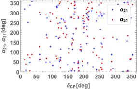
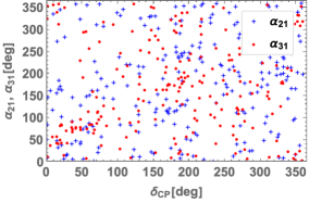
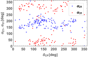
Figure 1: Plots of $\alpha_{12}$ and $\alpha_{31}$ for $\tau=\infty$ (left), $i$ (center) and $\omega$ (right), normal hierarchy case. Blue $+$ and Red $\bullet$ represent $\alpha_{12}$ and $\alpha_{31}$ for corresponding $\delta_{\mathrm{CP}}$, respectively.

In Fig. 1, scatter plots of $\alpha_{12}$ and $\alpha_{31}$ are shown. No specific tendency of the distribution is seen for $\tau=\infty,i$ case. For $\tau=\omega$ case, on the other hand, we can see $100^{\circ}<\alpha_{21}<250^{\circ}$ and $\alpha_{31}<100^{\circ},250^{\circ}<\alpha_{31}$ are favored.

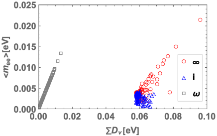
Figure 2: Plot of $\sum D_{v}$–$\langle m_{ee}\rangle$ for $\tau=\infty$, $i$ and $\omega$, normal hierarchy case.

In Fig. 2, scatter plot of $\sum D_{v}$–$\langle m_{ee}\rangle$ is shown. For $\tau=\infty$ case, parameter region $0.05<\sum D_{v}<0.1$ eV and $\langle m_{ee}\rangle<0.025$ eV is favored. For $\tau=i$ case, all the produced points in the numerical calculation is concentrated in $\sum D_{v}\sim 0.06$ eV and $\langle m_{ee}\rangle<0.005$ eV. For $\tau=\omega$ case, we can see $\langle m_{ee}\rangle$ seems to be propotional to $D_{v}$.

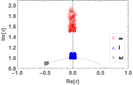
Figure 3: Scatter plot of Re[$\tau$]–Im[$\tau$] for $\tau=\infty$, $i$ and $\omega$, normal hierarchy case.

In Fig. 3, scatter plot of Re[$\tau$]–Im[$\tau$] is shown. Points correspond to $\tau=\infty$ case distribute in Re[$\tau$]$\sim 0$, also $1.5<$ Im[$\tau$] $<2$. For $\tau=i$ and $\omega$ cases, the distribution is more dense than $\tau=\infty$ case. Especially, $\tau=\omega$ points are located not on the real axis, i.e., Re[$\tau$]$\sim-0.5$.

III.2 Inverted Hierarchy Case

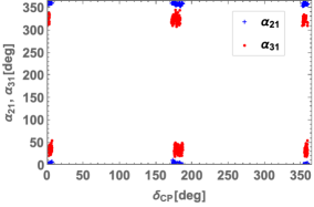
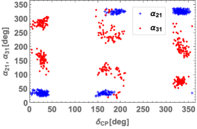
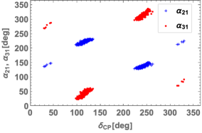
Figure 4: Legend is same as Fig. 1 but for inverted hierarchy case.

In Fig. 4, scatter plots of $\alpha_{21}$ and $\alpha_{31}$ for inverted hierarchy are shown. Unlike the normal hierarchy case, several specific regions are favored even for $\tau=\infty,i$ cases. Especially, in $\tau=\infty$ case, all the points are densely gathered in region $\delta_{\mathrm{CP}}\sim 0^{\circ}(360^{\circ}),180^{\circ}$ and $\alpha_{21},\alpha_{31}\sim 0^{\circ}(360^{\circ})$.

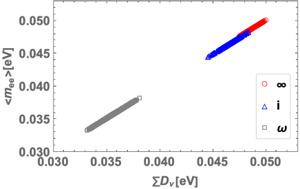
Figure 5: Legend is same as Fig. 2 but for inverted hierarchy case.

In Fig. 5, scatter plot of $\sum D_{v}$–$\langle m_{ee}\rangle$ is shown. For all cases, $\langle m_{ee}\rangle$ seems to be propotional to $D_{v}$. Range $0.032<\sum D_{v}<0.038$, $0.044<\sum D_{v}<0.049$ and $0.047<\sum D_{v}<0.05$ on the proportional function are favored for $\tau=\infty,i,\omega$ cases, respectively.

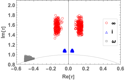
Figure 6: Legend is same as Fig. 3 but for inverted hierarchy case.

In Fig. 6, Scatter plot of Re[$\tau$]–Im[$\tau$] is shown. For $\tau=\infty,i$ cases, distributions are symmetric about the real axis. Points corresponds to $\tau=i$ case are converged on two narrow regions in small Im[$\tau$] region while points corresponds to $\tau=\infty$ widely spread in $1.3<$ Im[$\tau$] $<1.8$ compared to $\tau=i$ case. Distribution of $\tau=\omega$ is concentrated on Re[$\tau$] $\sim-0.5$ and Im[$\tau$] $\sim 0.9$, and not symmetric about the real axis.

IV Summary and Conclusions

We have proposed a lepton model under the modular $A_{4}$ and gauged $U(1)_{R}$ symmetries, in which the neutrino masses are induced at one-loop level. Also we have several predictions on the lepton sector thanks to the modular $A_{4}$ symmetry, especially, on the fixed points of $\tau=i,\omega,i\times\infty$. We especially point it out that we have found $100^{\circ}<\alpha_{21}<250^{\circ}$ and $\alpha_{31}<100^{\circ},250^{\circ}<\alpha_{31}$ are favored, and $0\lesssim\langle m_{ee}\rangle\lesssim 0.02$ eV seems be proportional to $D_{v}$ for $\tau=\omega$ with NH. And we have obtained more predictions for all the three cases with IH, as we have shown in the previous section. These cases would be verifiable and tested by future experiments soon.

Appendix

Here, we show several properties of modular $A_{4}$ symmetry. In general, the modular group $\bar{\Gamma}$ is a group of linear fractional transformation $\gamma$, acting on the modulus $\tau$ which belongs to the upper-half complex plane and transforms as

$$\tau\longrightarrow\gamma\tau=\frac{a\tau+b}{c\tau+d}\ ,~{}~{}{\rm where}~{}~{}a,b,c,d\in\mathbb{Z}~{}~{}{\rm and}~{}~{}ad-bc=1,~{}~{}{\rm Im}[\tau]>0~{}.$$ (60)

This is isomorphic to $PSL(2,\mathbb{Z})=SL(2,\mathbb{Z})/\{I,-I\}$ transformation. Then modular transformation is generated by two transformations $S$ and $T$ defined by:

$$S:\tau\longrightarrow-\frac{1}{\tau}\ ,\qquad\qquad T:\tau\longrightarrow\tau+1\ ,$$ (61)

and they satisfy the following algebraic relations,

$$S^{2}=\mathbb{I}\ ,\qquad(ST)^{3}=\mathbb{I}\ .$$ (62)

More concretely, we can fix the basis of $S$ and $T$ as follows:

$$S=\frac{1}{3}\begin{pmatrix}-1&2&2\\ -2&-1&2\\ 2&2&-1\\ \end{pmatrix},\quad T=\begin{pmatrix}1&0&0\\ 0&\omega&0\\ 0&0&\omega^{2}\\ \end{pmatrix},$$ (63)

where $\omega\equiv e^{2\pi i/3}$.

Here we introduce the series of groups $\Gamma(N)~{}(N=1,2,3,\dots)$ which are defined by

$$\begin{aligned} \Gamma(N)=\left\{\begin{pmatrix}a&b\\ c&d\end{pmatrix}\in SL(2,\mathbb{Z})~{},~{}~{}\begin{pmatrix}a&b\\ c&d\end{pmatrix}=\begin{pmatrix}1&0\\ 0&1\end{pmatrix}~{}~{}({\rm mod}~{}N)\right\}\end{aligned},$$ (64)

and we define $\bar{\Gamma}(2)\equiv\Gamma(2)/\{I,-I\}$ for $N=2$. Since the element $-I$ does not belong to $\Gamma(N)$ for $N>2$ case, we have $\bar{\Gamma}(N)=\Gamma(N)$, that are infinite normal subgroup of $\bar{\Gamma}$ known as principal congruence subgroups. We thus obtain finite modular groups as the quotient groups defined by $\Gamma_{N}\equiv\bar{\Gamma}/\bar{\Gamma}(N)$. For these finite groups $\Gamma_{N}$, $T^{N}=\mathbb{I}$ is imposed, and the groups $\Gamma_{N}$ with $N=2,3,4$ and $5$ are isomorphic to $S_{3}$, $A_{4}$, $S_{4}$ and $A_{5}$, respectively deAdelhartToorop:2011re .

Modular forms of level $N$ are holomorphic functions $f(\tau)$ which are transformed under the action of $\Gamma(N)$ given by

$$f(\gamma\tau)=(c\tau+d)^{k}f(\tau)~{},~{}~{}\gamma\in\Gamma(N)~{},$$ (65)

where $k$ is the so-called as the modular weight.

Under the modular transformation in Eq.(60) in case of $A_{4}$ ($N=3$) modular group, a field $\phi^{(I)}$ is also transformed as

$$\phi^{(I)}\to(c\tau+d)^{-k_{I}}\rho^{(I)}(\gamma)\phi^{(I)},$$ (66)

where $-k_{I}$ is the modular weight and $\rho^{(I)}(\gamma)$ denotes a unitary representation matrix of $\gamma\in\Gamma(2)$ ($A_{4}$ reperesantation). Thus Lagrangian such as Yukawa terms can be invariant if sum of modular weight from fields and modular form in corresponding term is zero (also invariant under $A_{4}$ and gauge symmetry).

The kinetic terms and quadratic terms of scalar fields can be written by

$$\sum_{I}\frac{|\partial_{\mu}\phi^{(I)}|^{2}}{(-i\tau+i\bar{\tau})^{k_{I}}}~{},\quad\sum_{I}\frac{|\phi^{(I)}|^{2}}{(-i\tau+i\bar{\tau})^{k_{I}}}~{},$$ (67)

which is invariant under the modular transformation and overall factor is eventually absorbed by a field redefinition consistently. Therefore the Lagrangian associated with these terms should be invariant under the modular symmetry.

The basis of modular forms with weight 2, $Y^{(2)}_{3}=(y_{1},y_{2},y_{3})$, transforming as a triplet of $A_{4}$ is written in terms of Dedekind eta-function $\eta(\tau)$ and its derivative Feruglio:2017spp :

$$y_{1}(\tau) =\frac{i}{2\pi}\left(\frac{\eta^{\prime}(\tau/3)}{\eta(\tau/3)}+\frac{\eta^{\prime}((\tau+1)/3)}{\eta((\tau+1)/3)}+\frac{\eta^{\prime}((\tau+2)/3)}{\eta((\tau+2)/3)}-\frac{27\eta^{\prime}(3\tau)}{\eta(3\tau)}\right)$$

$$\simeq 1+12q+36q^{2}+12q^{3}+\cdots,$$ (68)

$$y_{2}(\tau) =\frac{-i}{\pi}\left(\frac{\eta^{\prime}(\tau/3)}{\eta(\tau/3)}+\omega^{2}\frac{\eta^{\prime}((\tau+1)/3)}{\eta((\tau+1)/3)}+\omega\frac{\eta^{\prime}((\tau+2)/3)}{\eta((\tau+2)/3)}\right),$$

$$\simeq-6q^{1/3}(1+7q+8q^{2}+\cdots),$$ (69)

$$y_{3}(\tau) =\frac{-i}{\pi}\left(\frac{\eta^{\prime}(\tau/3)}{\eta(\tau/3)}+\omega\frac{\eta^{\prime}((\tau+1)/3)}{\eta((\tau+1)/3)}+\omega^{2}\frac{\eta^{\prime}((\tau+2)/3)}{\eta((\tau+2)/3)}\right)$$

$$\simeq-18q^{2/3}(1+2q+5q^{2}+\cdots),$$ (70)

where $q=e^{2\pi i\tau}$, and expansion form in terms of $q$ would sometimes be useful to have numerical analysis.

Then, we can construct the higher order of couplings $Y^{(4)}_{1},Y^{(6)}_{1},Y^{(10)}_{1},Y^{(6)}_{3},Y^{(6)}_{3^{\prime}}$ following the multiplication rules as follows:

$$Y^{(4)}_{1} =y^{2}_{1}+2y_{2}y_{3},\ Y^{(6)}_{1}=y^{3}_{1}+y^{3}_{2}+y^{3}_{3}-3y_{1}y_{2}y_{3},\ Y^{(10)}_{1}=Y^{(4)}_{1}Y^{(6)}_{1},$$ (71)

$$Y^{(6)}_{3} \equiv(y^{\prime}_{1},y^{\prime}_{2},y^{\prime}_{3})=(y^{3}_{1}+2y_{1}y_{2}y_{3},y_{1}^{2}y_{2}+2y^{2}_{2}y_{3},y^{2}_{1}y_{3}+2y^{2}_{3}y_{2}),$$ (72)

$$Y^{(6)}_{3^{\prime}} \equiv(y^{\prime\prime}_{1},y^{\prime\prime}_{2},y^{\prime\prime}_{3})=(y^{3}_{3}+2y_{1}y_{2}y_{3},y^{2}_{3}y_{1}+2y^{2}_{1}y_{2},y^{2}_{3}y_{2}+2y^{2}_{2}y_{1}),$$ (73)

where the above relations are constructed by the multiplication rules under $A_{4}$ as shown below:

$$\begin{pmatrix}a_{1}\\ a_{2}\\ a_{3}\end{pmatrix}_{\bf 3}\otimes\begin{pmatrix}b_{1}\\ b_{2}\\ b_{3}\end{pmatrix}_{\bf 3^{\prime}} =\left(a_{1}b_{1}+a_{2}b_{3}+a_{3}b_{2}\right)_{\bf 1}\oplus\left(a_{3}b_{3}+a_{1}b_{2}+a_{2}b_{1}\right)_{{\bf 1}^{\prime}}$$

$$\oplus\left(a_{2}b_{2}+a_{1}b_{3}+a_{3}b_{1}\right)_{{\bf 1}^{\prime\prime}}$$

$$\oplus\frac{1}{3}\begin{pmatrix}2a_{1}b_{1}-a_{2}b_{3}-a_{3}b_{2}\\ 2a_{3}b_{3}-a_{1}b_{2}-a_{2}b_{1}\\ 2a_{2}b_{2}-a_{1}b_{3}-a_{3}b_{1}\end{pmatrix}_{{\bf 3}}\oplus\frac{1}{2}\begin{pmatrix}a_{2}b_{3}-a_{3}b_{2}\\ a_{1}b_{2}-a_{2}b_{1}\\ a_{3}b_{1}-a_{1}b_{3}\end{pmatrix}_{{\bf 3^{\prime}}\ }\ ,$$

$${\bf 1}\otimes{\bf 1}={\bf 1}\ ,\quad {\bf 1^{\prime}}\otimes{\bf 1^{\prime}}={\bf 1^{\prime\prime}}\ ,\quad{\bf 1^{\prime\prime}}\otimes{\bf 1^{\prime\prime}}={\bf 1^{\prime}}\ ,\quad{\bf 1^{\prime}}\otimes{\bf 1^{\prime\prime}}={\bf 1}\ .$$ (74)

Finally, we show the features of fixed points of $\tau=i,\omega,i\times\infty$.

• In case of $\tau=i$, it is invariant under the transformation of $\tau\to-1/\tau$ that corresponds to $S$ transformation. It implies that there is a remnant $Z_{2}$ symmetry and its element is given by $\{1,S\}$. Then, the concrete value of $Y^{(2)}_{3}$ can be written down by Okada:2020ukr

  $$Y^{(2)}_{3} \simeq 1.0025(1,1-\sqrt{3},-2+\sqrt{3}).$$ (75)

• In case of $\tau=\omega$, it is invariant under the transformation of $\tau\to-1/(1+\tau)$ that corresponds to $ST$ transformation. It implies that there is a remnant $Z_{3}$ symmetry and its element is given by $\{1,ST,(ST)^{2}\}$. Then, the concrete value of $Y^{(2)}_{3}$ can be written down by Okada:2020ukr

  $$Y^{(2)}_{3} \simeq 0.9486(1,\omega,-\frac{1}{2}\omega^{2}).$$ (76)

• In case of $\tau=i\times\infty$, this corresponds to $T$ transformation. It suggests that there is a remnant $Z_{3}$ symmetry and its element is given by $\{1,T,T^{2}\}$. Then, the concrete value of $Y^{(2)}_{3}$ can be written down by Okada:2020ukr

  $$Y^{(2)}_{3} \simeq(1,0,0).$$ (77)

References

-
(1)
H. Baer, T. Barklow, K. Fujii, Y. Gao, A. Hoang, S. Kanemura, J. List, H. E. Logan, A. Nomerotski, M. Perelstein, M. E. Peskin, R. P
UTF00F6schl, J. Reuter, S. Riemann, A. Savoy-Navarro, G. Servant, T. M. P. Tait and J. Yu, [arXiv:1306.6352 [hep-ph]]. - (2) R. de Adelhart Toorop, F. Feruglio and C. Hagedorn, Nucl. Phys. B 858, 437 (2012) [arXiv:1112.1340 [hep-ph]].
- (3) F. Feruglio, arXiv:1706.08749 [hep-ph].
- (4) J. C. Criado and F. Feruglio, SciPost Phys. 5 (2018) no.5, 042 [arXiv:1807.01125 [hep-ph]].
- (5) T. Kobayashi, N. Omoto, Y. Shimizu, K. Takagi, M. Tanimoto and T. H. Tatsuishi, JHEP 1811, 196 (2018) [arXiv:1808.03012 [hep-ph]].
- (6) H. Okada and M. Tanimoto, Phys. Lett. B 791, 54 (2019) [arXiv:1812.09677 [hep-ph]].
- (7) T. Nomura and H. Okada, Phys. Lett. B 797 (2019), 134799 [arXiv:1904.03937 [hep-ph]].
- (8) H. Okada and M. Tanimoto, arXiv:1905.13421 [hep-ph].
- (9) F. J. de Anda, S. F. King and E. Perdomo, Phys. Rev. D 101 (2020) no.1, 015028 [arXiv:1812.05620 [hep-ph]].
- (10) P. P. Novichkov, S. T. Petcov and M. Tanimoto, Phys. Lett. B 793 (2019), 247-258 [arXiv:1812.11289 [hep-ph]].
- (11) T. Nomura and H. Okada, arXiv:1906.03927 [hep-ph].
- (12) G. J. Ding, S. F. King and X. G. Liu, JHEP 1909, 074 (2019) [arXiv:1907.11714 [hep-ph]].
- (13) H. Okada and Y. Orikasa, arXiv:1907.13520 [hep-ph].
- (14) T. Nomura, H. Okada and O. Popov, Phys. Lett. B 803 (2020), 135294 [arXiv:1908.07457 [hep-ph]].
- (15) T. Kobayashi, Y. Shimizu, K. Takagi, M. Tanimoto and T. H. Tatsuishi, Phys. Rev. D 100 (2019) no.11, 115045 [arXiv:1909.05139 [hep-ph]].
- (16) T. Asaka, Y. Heo, T. H. Tatsuishi and T. Yoshida, JHEP 01 (2020), 144 [arXiv:1909.06520 [hep-ph]].
- (17) D. Zhang, Nucl. Phys. B 952 (2020), 114935 [arXiv:1910.07869 [hep-ph]].
- (18) G. J. Ding, S. F. King, X. G. Liu and J. N. Lu, JHEP 12 (2019), 030 [arXiv:1910.03460 [hep-ph]].
- (19) T. Nomura, H. Okada and S. Patra, [arXiv:1912.00379 [hep-ph]].
- (20) T. Kobayashi, T. Nomura and T. Shimomura, [arXiv:1912.00637 [hep-ph]].
- (21) X. Wang, [arXiv:1912.13284 [hep-ph]].
- (22) H. Okada and Y. Shoji, [arXiv:2003.13219 [hep-ph]].
- (23) H. Okada and M. Tanimoto, [arXiv:2005.00775 [hep-ph]].
- (24) M. K. Behera, S. Singirala, S. Mishra and R. Mohanta, [arXiv:2009.01806 [hep-ph]].
- (25) M. K. Behera, S. Mishra, S. Singirala and R. Mohanta, [arXiv:2007.00545 [hep-ph]].
- (26) T. Nomura and H. Okada, [arXiv:2007.04801 [hep-ph]].
- (27) T. Nomura and H. Okada, [arXiv:2007.15459 [hep-ph]].
- (28) T. Asaka, Y. Heo and T. Yoshida, [arXiv:2009.12120 [hep-ph]].
- (29) H. Okada and M. Tanimoto, [arXiv:2009.14242 [hep-ph]].
- (30) T. Kobayashi, K. Tanaka and T. H. Tatsuishi, Phys. Rev. D 98 (2018) no.1, 016004 [arXiv:1803.10391 [hep-ph]].
- (31) T. Kobayashi, Y. Shimizu, K. Takagi, M. Tanimoto, T. H. Tatsuishi and H. Uchida, Phys. Lett. B 794, 114 (2019) [arXiv:1812.11072 [hep-ph]].
- (32) T. Kobayashi, Y. Shimizu, K. Takagi, M. Tanimoto and T. H. Tatsuishi, PTEP 2020 (2020) no.5, 053B05 [arXiv:1906.10341 [hep-ph]].
- (33) H. Okada and Y. Orikasa, arXiv:1907.04716 [hep-ph].
- (34) S. Mishra, [arXiv:2008.02095 [hep-ph]].
- (35) J. T. Penedo and S. T. Petcov, Nucl. Phys. B 939, 292 (2019) [arXiv:1806.11040 [hep-ph]].
- (36) P. P. Novichkov, J. T. Penedo, S. T. Petcov and A. V. Titov, JHEP 1904, 005 (2019) [arXiv:1811.04933 [hep-ph]].
- (37) T. Kobayashi, Y. Shimizu, K. Takagi, M. Tanimoto and T. H. Tatsuishi, arXiv:1907.09141 [hep-ph].
- (38) S. F. King and Y. L. Zhou, Phys. Rev. D 101 (2020) no.1, 015001 [arXiv:1908.02770 [hep-ph]].
- (39) H. Okada and Y. Orikasa, arXiv:1908.08409 [hep-ph].
- (40) J. C. Criado, F. Feruglio and S. King, J.D., JHEP 02 (2020), 001 [arXiv:1908.11867 [hep-ph]].
- (41) X. Wang and S. Zhou, JHEP 05 (2020), 017 [arXiv:1910.09473 [hep-ph]].
- (42) P. P. Novichkov, J. T. Penedo, S. T. Petcov and A. V. Titov, JHEP 04 (2019), 174 [arXiv:1812.02158 [hep-ph]].
- (43) G. J. Ding, S. F. King and X. G. Liu, Phys. Rev. D 100 (2019) no.11, 115005 [arXiv:1903.12588 [hep-ph]].
- (44) A. Baur, H. P. Nilles, A. Trautner and P. K. S. Vaudrevange, Phys. Lett. B 795 (2019), 7-14 [arXiv:1901.03251 [hep-th]].
- (45) I. de Medeiros Varzielas, S. F. King and Y. L. Zhou, Phys. Rev. D 101 (2020) no.5, 055033 [arXiv:1906.02208 [hep-ph]].
- (46) X. G. Liu and G. J. Ding, JHEP 1908 (2019) 134 [arXiv:1907.01488 [hep-ph]].
- (47) P. Chen, G. J. Ding, J. N. Lu and J. W. F. Valle, arXiv:2003.02734 [hep-ph].
- (48) P. P. Novichkov, J. T. Penedo and S. T. Petcov, [arXiv:2006.03058 [hep-ph]].
- (49) X. G. Liu, C. Y. Yao and G. J. Ding, [arXiv:2006.10722 [hep-ph]].
- (50) S. Kikuchi, T. Kobayashi, H. Otsuka, S. Takada and H. Uchida, [arXiv:2007.06188 [hep-th]].
- (51) G. Altarelli and F. Feruglio, Rev. Mod. Phys. 82 (2010) 2701 [arXiv:1002.0211 [hep-ph]].
- (52) H. Ishimori, T. Kobayashi, H. Ohki, Y. Shimizu, H. Okada and M. Tanimoto, Prog. Theor. Phys. Suppl. 183 (2010) 1 [arXiv:1003.3552 [hep-th]].
- (53) H. Ishimori, T. Kobayashi, H. Ohki, H. Okada, Y. Shimizu and M. Tanimoto, Lect. Notes Phys. 858 (2012) 1, Springer.
- (54) D. Hernandez and A. Y. Smirnov, Phys. Rev. D 86 (2012) 053014 [arXiv:1204.0445 [hep-ph]].
- (55) S. F. King and C. Luhn, Rept. Prog. Phys. 76 (2013) 056201 [arXiv:1301.1340 [hep-ph]].
- (56) S. F. King, A. Merle, S. Morisi, Y. Shimizu and M. Tanimoto, arXiv:1402.4271 [hep-ph].
- (57) S. F. King, Prog. Part. Nucl. Phys. 94 (2017) 217 [arXiv:1701.04413 [hep-ph]].
- (58) S. T. Petcov, Eur. Phys. J. C 78 (2018) no.9, 709 [arXiv:1711.10806 [hep-ph]].
- (59) A. Baur, H. P. Nilles, A. Trautner and P. K. S. Vaudrevange, Nucl. Phys. B 947 (2019), 114737 [arXiv:1908.00805 [hep-th]].
- (60) T. Kobayashi, Y. Shimizu, K. Takagi, M. Tanimoto, T. H. Tatsuishi and H. Uchida, Phys. Rev. D 101 (2020) no.5, 055046 [arXiv:1910.11553 [hep-ph]].
- (61) P. P. Novichkov, J. T. Penedo, S. T. Petcov and A. V. Titov, JHEP 07 (2019), 165 [arXiv:1905.11970 [hep-ph]].
- (62) M. C. Chen, S. Ramos-Sánchez and M. Ratz, Phys. Lett. B 801 (2020), 135153 [arXiv:1909.06910 [hep-ph]].
- (63) I. de Medeiros Varzielas, M. Levy and Y. L. Zhou, [arXiv:2008.05329 [hep-ph]].
- (64) K. I. Nagao and H. Okada, [arXiv:2008.13686 [hep-ph]].
- (65) T. Kobayashi and H. Otsuka, Phys. Rev. D 102, no.2, 026004 (2020) doi:10.1103/PhysRevD.102.026004 [arXiv:2004.04518 [hep-th]].
- (66) T. Nomura and H. Okada, Phys. Lett. B 761, 190-196 (2016) doi:10.1016/j.physletb.2016.08.023 [arXiv:1606.09055 [hep-ph]].
- (67) E. Ma, Phys. Rev. D 73, 077301 (2006) doi:10.1103/PhysRevD.73.077301 [arXiv:hep-ph/0601225 [hep-ph]].
- (68) Z. Maki, M. Nakagawa and S. Sakata, Prog. Theor. Phys. 28, 870-880 (1962) doi:10.1143/PTP.28.870
- (69) A. Gando et al. [KamLAND-Zen], Phys. Rev. Lett. 117, no.8, 082503 (2016) doi:10.1103/PhysRevLett.117.082503 [arXiv:1605.02889 [hep-ex]].
- (70) I. Esteban, M. C. Gonzalez-Garcia, A. Hernandez-Cabezudo, M. Maltoni and T. Schwetz, JHEP 01, 106 (2019) doi:10.1007/JHEP01(2019)106 [arXiv:1811.05487 [hep-ph]].
- (71) A. M. Baldini et al. [MEG], Eur. Phys. J. C 76, no.8, 434 (2016) doi:10.1140/epjc/s10052-016-4271-x [arXiv:1605.05081 [hep-ex]].
- (72) J. Adam et al. [MEG], Phys. Rev. Lett. 110, 201801 (2013) doi:10.1103/PhysRevLett.110.201801 [arXiv:1303.0754 [hep-ex]].
- (73) K. Hagiwara, R. Liao, A. D. Martin, D. Nomura and T. Teubner, J. Phys. G 38, 085003 (2011) doi:10.1088/0954-3899/38/8/085003 [arXiv:1105.3149 [hep-ph]].