Pattern formation in clouds via Turing instabilities

Abstract

Pattern formation in clouds is a well-known feature, which can be observed almost every day. However, the guiding processes for structure formation are mostly unknown, and also theoretical investigations of cloud patterns are quite rare. From many scientific disciplines the occurrence of patterns in non-equilibrium systems due to Turing instabilities is known, i.e. unstable modes grow and form spatial structures. In this study we investigate a generic cloud model for the possibility of Turing instabilities. For this purpose, the model is extended by diffusion terms. We can show that for some cloud models, i.e special cases of the generic model, no Turing instabilities are possible. However, we also present a general class of cloud models, where Turing instabilities can occur. A key requisite is the occurrence of (weakly) nonlinear terms for accretion. Using numerical simulations for a special case of the general class of cloud models, we show spatial patterns of clouds in one and two spatial dimensions. From the numerical simulations we can see that the competition between collision terms and sedimentation is an important issue for the existence of pattern formation.

1 Introduction

Pattern formation is a general feature in nature. We find patterns in many different locations and research fields, e.g. sand ripples at sand dunes or at the beach, stripes on zebras and fishes, convective cells in Rayleigh-Benard convection, spiral states in chemical reaction systems as e.g. the famous Belousov–Zhabotinski system, and many other examples. The generation of structures is a common feature for systems out of thermodynamic equilibrium. In contrast to states at equilibrium, which tend to be homogeneous, an external forcing driving a system out of equilibrium has the potential to form new structures. These structures can have different forms, i.e. homogeneous or inhomogeneous in space and stationary or oscillatory in time (see, e.g.,[Cross, M. C., Hohenberg, P. C. (1993)]). Pattern formation is an emergent process, and is usually not predictable a priori from the underlying micro states of the system; the structures on larger scales often appear in a spontaneous way. Research on pattern formation is an important field in many disciplines in natural sciences e.g. mathematical biology [Murray, J. D. (2003)], chemistry [Kondepudi, D. and Prigogine, I. (2015)], fluid dynamics (e.g. Rayleigh-Benard convection, see [Bodenschatz, E. et al. (2000)]) and many other fields.

There are several approaches to represent pattern formation in models. One of the first approaches was presented by [Turing, A. M. (1952)] in his seminal article on morphogenesis. Chemical reactions are represented by a system of ordinary differential equations (ODEs). This set of equations is extended by diffusion terms, i.e. a Laplacian in spatial directions is added to each equation representing the concentration of a chemical species. It can be shown by linear stability analysis that under certain conditions (e.g. different diffusion coefficients) stable stationary points of the ODE system can be destabilised, i.e. some Fourier modes become unstable and grow, until they become saturated by nonlinear effects. Since only wave numbers out of a finite interval become unstable, spatial structures become visible. This phenomenon is called Turing instability. There are other attempts to represent structures in models; a whole zoo of structure equations is available [Cross, M. C., Hohenberg, P. C. (1993)]. However, these approaches are often empirical and the variables are not directly linked to physical quantities. Sometimes, it is possible to reduce or reformulate an underlying physical system of equations to a known structure equation ([Monroy, D. L. and Naumis, G. G. (2020)]). The approach of using reaction-diffusion equations is more direct, but often ignores other feedback due to the simplistic starting point. Nevertheless, reaction-diffusion equations provide an important class of equations for pattern formation, and are directly linked to the physical variables.

In atmospheric physics, a very prominent example of emerging structures is pattern formation in clouds, which can be seen nicely from surface observation as well as obtained by remote sensing techniques (e.g. from satellites). Surprisingly, the investigation of pattern formation in clouds is currently not a widespread topic in atmospheric physics. During the 1980s and 1990s several investigations and empirical studies on pattern formation in liquid clouds were carried out, see e.g. the review on cloud streets in the planetary boundary layer [Etling, D. and Brown, R. (1993)] or the series on cloud clustering [Weger, R. et al (1992), Zhu et al (1992), Weger, R. et al (1993), Lee, J. et al. (1994), Nair, U. et al. (1998)]. There are only few newer studies on pattern formation, mainly in connection with investigations of open and closed cells in marine stratocumulus (see, e.g., [Glassmeier, F. and Feingold, G. (2017), Khouider, B. and Bihlo, A. (2019)]); however, rigorous and theoretic investigations on the formation of patterns for clouds are lacking. This is surprising, since internal structures of clouds constitute a serious uncertainty in terms of radiative feedback. Radiative transfer in homogeneous media is completely different than in inhomogeneous media. For the investigations of Earth’s energy budget, clouds play a major role due to scattering and reflection of sunlight as well as trapping infrared radiation by absorption and re-emission. In structured clouds, many assumptions of radiative transfer in homogeneous media do not work anymore; for instance multiple scattering occurs frequently, and horizontal radiative transport becomes more important. Thus, in this respect the investigation of structured (i.e. inhomogeneous) clouds and their origin and evolution is quite essential for meaningful estimations of cloud radiative forcings.

There is another difficulty concerning the representation of cloud patterns in models. Clouds constitute an ensemble of many water particles. In cloud physics, one often considers processes on the scale of individual particles, which are only partly understood until now. The description of the statistical ensemble of cloud particles, forming the macroscopic “object” cloud, is not very precise, and is lacking a rigorous formulation. There are some attempts based on Boltzmann-type evolution equations (see, e.g., [Morrison, H. et al. (2020)], [Beheng, K. D. (2010)]) ,however there is no general theory of clouds and no basic set of equations as a common ground to start is available in cloud physics. In contrast when the motion of dry air shall be described, the Navier-Stokes equations can be used. For the description of clouds, often averaged variables such as the number concentration or mass concentration of particles are used. It is possible to relate these quantities to general moments of the underlying size/mass distribution of the particle ensemble ( see, e.g. [Beheng, K. D. (2010)], [Khain, A. P. et al. (2015)]). For these averaged variables, the process rates of the cloud processes are often formulated by nonlinear terms. With these parameterisation at hand the temporal evolution of the averaged quantities can be described by system of ordinary differential equations, where the process rates form the right hand side of the ODE system, also called the reaction term. Since a basic theory is lacking, the formulation of the process rates differ among the available cloud models, and often they are not mathematically consistent. For instance, the uniqueness of solutions of the ODE system is not always guaranteed, and often requires a more rigorous treatment (see, e.g.,[Hanke, M, and Porz, N. (2020)]). Nevertheless, these cloud models are often used, and they are useful for scientific investigations as well as for operational weather forecasts or climate predictions.

In this study, we investigate the potential of generic cloud models, formulated in a former study ([Rosemeier, J. et al. (2018)]), to form spatial structures. We couple the model equations with diffusion terms, i.e. Laplacians in the spatial directions; this leads to reaction-diffusion equations for cloud physics schemes, which will be investigated in terms of Turing instabilities.

The study is structured as follows: In the next section we will briefly describe the generic cloud model and the represented processes. In section 3 we present the approach of linear stability theory, leading to conditions for Turing instabilities in reaction-diffusion equations. The generic cloud model always allows a trivial equilibrium (no clouds, only rain); in section 4 we show that this equilibrium state cannot form Turing instabilities. In section 5 we present a special case of a cloud model, which does not show pattern formation; this case contains standard cloud models. In contrast, in section 6 we present a general class of cloud models allowing Turing instabilities and thus pattern formation. In addition, a special case is explored for investigating several features of the model. In the following section 7 this cloud model is numerically simulated for a 1D and a 2D scenario, and these results are shown. We end the study with a summary and some conclusions.

2 Generic cloud model

We present the generic cloud model formulated in the former study by [Rosemeier, J. et al. (2018)]. The model represents clouds consisting exclusively of liquid water droplets, so-called warm clouds. The droplet population is divided into two different regimes, namely cloud droplets and rain drops, respectively. Cloud droplets are water droplets of small sizes (radius smaller than $\sim$40\text{\,}\mathrm{\SIUnitSymbolMicro m}$$), whereas rain drops are larger water particles. This separation can be seen in detailed simulations (see, e.g., [Beheng, K. D. (2010)] his figure 4), and partly in measurements. All water particles fall in vertical direction due to gravity. Since for small droplets the fall velocities are very small due to friction of air, we can assume that these droplets are stationary, in contrast to large rain drops, which fall out faster. This separation was first proposed by [Kessler, E. (1969)] in an ad hoc manner; however, it could be justified by the simulations mentioned above. We consider the mass concentrations of these two populations as variables in the model. The phase transitions (water vapour vs. liquid water) are guided by the saturation ratio $S_{l}=\frac{p_{v}}{p_{s}(T)}$, i.e. the ratio of partial pressure of water vapour, $p_{v}$, and its temperature dependent saturation vapour pressure, $p_{s}(T)$. Thermodynamic equilibrium, i.e. coexistence of gaseous and liquid water, is then fulfilled at $S_{l}=1$; for simplification of the notation, we also introduce the supersaturation $S:=S_{l}-1$, i.e. equilibrium is reached for $S=0$. For liquid clouds, the following processes must be taken into account.

• Condensation and diffusional growth/evaporation
  Cloud droplets are formed at thermodynamic conditions slightly beyond thermodynamic equilibrium, i.e. at supersaturation ($S>0$); actually, aerosol particles are activated and after passing a critical size, as given by Köhler theory ([Köhler, H. (1936)]), they constitute cloud droplets. In simple cloud models, this process of condensation is simplified and represented together with diffusional growth. Cloud droplets can grow or shrink by uptake or evaporation of water vapour, which is provided by diffusion; this process is also driven by the supersaturation, which controls the thermodynamic equilibrium. Diffusional growth is quite inefficient for large droplets, thus this process is only relevant for small droplets, i.e. for the cloud droplet category. Both processes, condensation and diffusional growth (or on the contrary evaporation for $S<0$) are represented by a rate $C=c^{\prime}Sq_{c}$ with a suitable constant $c^{\prime}$ depending on temperature and pressure only. For simplification, we assume in our investigations a permanent source of supersaturation, e.g. driven by a vertical upward motion. Thus, we can also neglect evaporation of water droplets for the system.

• Collision processes
  Since water particles fall with different velocities depending on their masses, there will be collisions between neighbouring particles of different size, and these particles will eventually form a single droplet after collision (so-called collision-coalescence). Because of the artificial splitting of the whole droplet ensemble into two categories, we have to consider two (artificial) processes:
  (1) Two cloud droplets collide and form a large rain drop; this process is called autoconversion. (2) A large rain drop collects a small cloud droplet by collision; this process is called accretion. These processes are usually modelled in the spirit of population dynamics, using nonlinear terms; however, derivations from integrals over size/mass distributions lead to similar descriptions (see, e.g., [Seifert, A. and Beheng, K. D. (2006)], [Beheng, K. D. (2010)]. Autoconversion can be represented by terms $A_{1}=a_{1}q_{c}^{\gamma}$ with a suitable constant $a_{1}>0$ and an exponent $\gamma>0$. For accretion, the terms can be formulated as $A_{2}=a_{2}q_{c}^{\beta_{c}}q_{r}^{\beta_{r}}$ with a suitable constant $a_{2}>0$ and exponents $\beta_{c},\beta_{r}>0$, mimicking a generalised predator-prey process.

• Sedimentation of particles
  For the representation of rain drops falling out of a cloud level, in general we would have to consider a hyperbolic term in the vertical direction. For simplicity, we assume just one atmospheric layer with a prescribed vertical extension. Thus, we discretise the hyperbolic term and assume a constant flux of mass from above. Then, the sedimentation term can be approximated by $D=B-dq_{r}^{\zeta}$, with constants $B,d>0$ and an exponent $\zeta>0$. Note, that terminal velocities of cloud particles can be parameterised by power laws (see, e.g., [Seifert, A. et al. (2014)]).

Using the representation of the processes as stated above, we obtain the generic cloud scheme described in [Rosemeier, J. et al. (2018)]:

$$\derivative{q_{c}}{t} =c^{\prime}Sq_{c}-a_{1}q_{c}^{\gamma}-a_{2}q_{c}^{\beta_{c}}q_{r}^{\beta_{r}},$$ (1a)

$$\derivative{q_{r}}{t} =\ \quad\qquad a_{1}q_{c}^{\gamma}+a_{2}q_{c}^{\beta_{c}}q_{r}^{\beta_{r}}+B-dq_{r}^{\zeta}.$$ (1b)

To simplify the notation we will write $c$ instead of $c^{\prime}S$ in the remaining of the study. For the analysis of the equations, we assume constant environmental conditions, i.e. constant temperature, pressure, and supersaturation ($S>0$), respectively. This assumption leads to an idealised situation, however it could be shown that similar conditions can be encountered in the atmosphere (see, e.g., [Korolev, A.V. and Mazin, I.P. (2003)])for quite long times. Assuming these constant conditions allows us to investigate the asymptotic states of the system.

The ODE system (1) was discussed in detail in [Rosemeier, J. et al. (2018)]. In the presented work the equations (1) are extended by diffusion terms, so we obtain the following system

$$\derivative{q_{c}}{t} =cq_{c}-a_{1}q_{c}^{\gamma}-a_{2}q_{c}^{\beta_{c}}q_{r}^{\beta_{r}}\qquad\qquad\quad+D_{1}\laplacian q_{c}$$ (2a)

$$\derivative{q_{r}}{t} =\ \ \quad\quad a_{1}q_{c}^{\gamma}+a_{2}q_{c}^{\beta_{c}}q_{r}^{\beta_{r}}-dq_{r}^{\zeta}+B+D_{2}\laplacian q_{r}.$$ (2b)

This is a reaction-diffusion system (or Turing system). Note, that the added diffusion terms do not represent molecular dynamics, as in chemical systems. Actually, these terms can be seen as a representation of unresolved (dynamical) processes, as e.g. small eddies or turbulence. For the representation of turbulence in subgrid scale schemes or entrainment due to unresolved eddies, often gradient terms are used (see, e.g.,[Deardorff, J. W. (1972)], [Stull, R. B. (1988)]). This approach leads to diffusion terms in the equations for the mean variables. The different values of the diffusion constants for the two water species can be motivated as follows:

Small clouds droplets will mainly follow the small scale motions in the system, thus the diffusion coefficient $D_{1}$ for this species should be large. On the other hand, rain drops are mostly accelerated by gravity, thus they are less affected by small scale motions. For this species, the diffusion coefficient $D_{2}$ can be chosen different from the coefficient $D_{1}$, e.g. we would assume $D_{2}<D_{1}$.

In the sequel the system (2) is investigated with respect to pattern formation. The occurrence of patterns cannot be guaranteed for the generic model, i.e. for all possible choices of parameters, but in some cases linear stability analysis predicts pattern formation. These findings can be confirmed by numerical simulations. In addition, numerical simulations with an extended parameter range might lead to further insights into potential pattern formation.

3 Linear stability analysis

The ideas of linear stability analysis (e.g. [Turing, A. M. (1952)]) can be used for the determination of stable and unstable modes of the system of equations. A classical example for the analysis of reaction-diffusion equations using linear stability analysis is the investigation of the Brusselator as a simple system describing chemical reactions (see, e.g., [Cross, M. and Greenside, H. (2009)] pp. 105-108). In this section we mostly follow the exposition given in [Cross, M. and Greenside, H. (2009)] for a 2D system of reaction-diffusion equations, as, e.g., given by (2).
The subsequent 2D reaction-diffusion system is given by

$$\derivative{u_{1}}{t} =f_{1}\quantity(u_{1},u_{2})+D_{1}\laplacian u_{1}$$ (3a)

$$\derivative{u_{2}}{t} =f_{2}\quantity(u_{1},u_{2})+D_{2}\laplacian u_{2}.$$ (3b)

In a first step, we determine the stationary and homogeneous equilibrium states, thus we omit the diffusion terms. By neglecting the Laplacians, we obtain a system of ordinary differential equations

$$\derivative{u_{1}}{t} =f_{1}\quantity(u_{1},u_{2})$$ (4a)

$$\derivative{u_{2}}{t} =f_{2}\quantity(u_{1},u_{2}).$$ (4b)

The right hand side is called the reaction term. We want to derive conditions for a stable equilibrium of (4) which can be destabilised by diffusion terms. First, we consider an equilibrium solution $u_{e1},u_{e2}$ of the system (4). By definition it satisfies the equations

$$0 =f_{1}\quantity(u_{e1},u_{e2})$$ (5a)

$$0 =f_{2}\quantity(u_{e1},u_{e2}).$$ (5b)

Next we compute the Jacobian of (4) evaluated at the equilibrium solution $u_{e1},u_{e2}$

$$Df|_{\quantity(u_{e1},u_{e2})}=\begin{pmatrix}a_{11}&a_{12}\\ a_{21}&a_{22}\\ \end{pmatrix},$$ (6)

where the entries of the matrix are determined by

$$a_{ij}=\partialderivative{f_{i}}{u_{j}}\quantity(u_{e1},u_{e2}).$$ (7)

The (potentially complex) eigenvalues of the Jacobian at the equilibrium state are denoted by $\sigma_{1},\sigma_{2}$. The equilibrium solution $u_{e1},u_{e2}$ is asymptotically stable if and only if the following relations are fulfilled

$$\text{tr}\quantity(Df) \coloneqq a_{11}+a_{22}=\sigma_{1}+\sigma_{2}<0$$ (8a)

$$\text{det}\quantity(Df) \coloneqq a_{11}a_{22}-a_{12}a_{21}=\sigma_{1}\cdot\sigma_{2}>0.$$ (8b)

This is equivalent to the more common condition for asymptotic stability, i.e. $\real(\sigma_{i})<0$ for $i=1,2$.

Now we consider the system (3) including the diffusion terms. For this purpose, we use spatial coordinates $x=(x_{1},\ldots,x_{n})^{T}$ and a generalised wave number vector $k=(k_{1},\ldots,k_{n})^{T}$. For each spatial direction, we consider linear waves with wave lengths $\lambda_{i}=\frac{2\pi}{k_{i}}$. The Laplacian is defined by $\displaystyle\laplacian=\sum_{i=1}^{n}\partialderivative[2]{\leavevmode\nobreak\ }{x_{i}}$. The spatial dimension is given by $n\geq 1$.

For the linear stability analysis of the reaction-diffusion system, we replace the reaction term by its linearisation evaluated at $u_{e1},u_{e2}$, i.e. with the linearisation $u=u_{e}+u_{p}$, with a small perturbation $u_{p}$ around the constant equilibrium state $u_{e}$, we obtain

$$\partialderivative{u_{p1}}{t} =a_{11}u_{p1}+a_{12}u_{p2}+D_{1}\laplacian u_{p1}$$ (9a)

$$\partialderivative{u_{p2}}{t} =a_{21}u_{p1}+a_{22}u_{p2}+D_{2}\laplacian u_{p2}.$$ (9b)

We want to derive conditions for the destabilisation of $u_{e1},u_{e2}$ due to the diffusion terms. For simplification we assume periodic boundary conditions; therefore a Fourier discretisation in space with a superposition of linear wave modes $\exp(ikx)$ can be applied. The system (9) shall be solved by a separation ansatz

$$u_{p}=\begin{pmatrix}u_{1q}\\ u_{2q}\\ \end{pmatrix}\exp(\sigma_{q}t)\exp(ikx).$$ (10)

using the eigenvalues $\sigma_{q}$ representing a single Fourier mode. Such a Fourier mode is an eigenfunction of the Laplacian, hence the equation

$$\laplacian\exp(ikx)=-\left(\sum_{i=1}^{n}k_{i}^{2}\right)\exp(ikx)=-q^{2}\exp(ikx)$$ (11)

holds, with the sum over all squared wave numbers $q^{2}=\sum k_{i}^{2}$, which is used as an index. Substituting (11) into the linearized equation (9) leads to the eigenvalue problem

$$Df_{q}\,u_{q}=\sigma_{q}u_{q},$$ (12)

for the coefficient $u_{q}$ of the Fourier mode (10) where the matrix $Df_{q}$ is given by

$$Df_{q}=\begin{pmatrix}a_{11}-D_{1}q^{2}&a_{12}\\ a_{21}&a_{22}-D_{2}q^{2}\\ \end{pmatrix}.$$ (13)

For the determination of the eigenvalues $\sigma_{q}$ of the matrix $Df_{q}$ the roots of the quadratic polynomial

$$0=\det(Df_{q}-\sigma_{q}I)=\sigma_{q}^{2}-\quantity(\tr(Df_{q}))\sigma_{q}+\det(Df_{q}).$$ (14)

must be determined. The eigenvalues $\sigma_{qi}$ are given by

$$\sigma_{q1/2}=\frac{1}{2}\tr(Df_{q})\pm\frac{1}{2}\sqrt{\quantity(\tr(Df_{q}))^{2}-4\det(Df_{q})}.$$ (15)

It follows that the mode which belongs to the wave number $q$ is asymptotically stable if and only if

$$\tr(Df_{q}) \coloneqq a_{11}+a_{22}-\quantity(D_{1}+D_{2})q^{2}=\sigma_{q1}+\sigma_{q2}<0$$ (16a)

$$\det(Df_{q}) \coloneqq\quantity(a_{11}-D_{1}q^{2})\quantity(a_{22}-D_{2}q^{2})-a_{12}a_{21}=\sigma_{q1}\cdot\sigma_{q2}>0.$$ (16b)

Remember, that the condition can also be formulated in terms of determinant and trace of the original ODE system, i.e.

$$\tr(Df_{q}) \coloneqq\tr(Df)-(D_{1}+D_{2})q^{2}$$ (17a)

$$\det(Df_{q}) \coloneqq\det(Df)-\quantity(D_{1}a_{22}+D_{2}a_{11})q^{2}+D_{1}D_{2}q^{4}$$ (17b)

We are interested in conditions for the destabilisation of a mode $q$. Equation (16a) is satisfied because equation (8a) is valid and $D_{1},D_{2},q^{2}>0$. The only way for destabilisation is to violate condition (16b), thus we look for a mode which fulfills

$$\quantity(a_{11}-D_{1}q^{2})\quantity(a_{22}-D_{2}q^{2})-a_{12}a_{21}<0.$$ (18)

The left hand side of (18) defines a quadratic polynomial in $q^{2}$,

$$p_{2}(q^{2})=\quantity(a_{11}-D_{1}q^{2})\quantity(a_{22}-D_{2}q^{2})-a_{12}a_{21}.$$ (19)

All modes $q$ with $p_{2}(q^{2})<0$ are unstable. The quadratic polynomial admits a minimum at

$$q_{m}^{2}=\frac{D_{1}a_{22}+D_{2}a_{11}}{2D_{1}D_{2}},$$ (20)

which constitutes the “most unstable” Fourier mode. Inserting the relation (20) into (18) yields the condition

$$D_{1}a_{22}+D_{2}a_{11}>2\sqrt{D_{1}D_{2}\quantity(a_{11}a_{22}-a_{12}a_{21})}$$ (21)

or in the reformulated version

$$D_{1}a_{22}+D_{2}a_{11}>2\sqrt{D_{1}D_{2}\det(Df)}$$ (22)

There is a chance to find an unstable mode $q$ if (21) holds, see figure 1. The conditions (8a) and (21) can be satisfied when $a_{11}$ and $a_{22}$ have opposite signs.

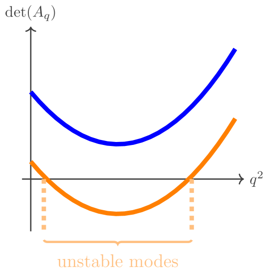
Figure 1: The quadratic polynomial (19), which gives the determinant of the Jacobian (13), is shown. No unstable modes occur if the minimum of $p_{2}$ is positive (blue line). Unstable modes are possible if the minimum of $p_{2}$ is negative (orange line).

4 The trivial equilibrium of the generic cloud model

We now show that the trivial equilibrium of the generic cloud model (1) in case of a stable stationary point never leads to Turing instabilities. We start with the generic cloud model (1), leading to the stationary point

$$q_{ce}=0,\leavevmode\nobreak\ q_{re}=\left(\frac{B}{d}\right)^{\frac{1}{\zeta}}.$$ (23)

Since this implies no cloud, just rain, in the atmospheric layer, this state is called trivial equilibrium. Actually, this stationary point is only valid for linear stability analysis for values of the exponents $\gamma\geq 1$ and $\beta_{c}\geq 1$. Otherwise, the partial derivatives with respect to $q_{c}$ do not exist at $q_{c}=0$. Cloud models with $\gamma<1$ or $\beta_{c}<1$ also lack Lipschitz continuity. Therefore, the Picard-Lindelöff theorem does not guarantee the unique solvability of the ODE system when the initial value for $q_{c}$ is given by $q_{c}=0$. For discussions of such cloud models and possible extensions to uniqueness, see the recent study by [Hanke, M, and Porz, N. (2020)]. In the remainder of the study developed here we will always assume $\gamma\geq 1,\beta_{c}\geq 1$. For linear stability analysis we have to consider the Jacobian $Df|_{(q_{ce},q_{re})}$. As discussed by [Rosemeier, J. et al. (2018)] the Jacobian always has the form

$$Df|_{(q_{ce},q_{re})}=\begin{pmatrix}a_{11}&0\\ a_{21}&a_{22}\\ \end{pmatrix}\coloneqq A,$$ (24)

with $a_{22}=-d\zeta\left(\frac{B}{d}\right)^{\frac{\zeta-1}{\zeta}}<0$. As $\beta_{c}\geq 1$ is assumed, we obtain $a_{12}=0$. If even the conditions $\gamma>1$ and $\beta_{c}>1$ hold, we obtain $a_{21}=0$, otherwise $a_{12}>0$; for details, see calculations in appendix A. Nevertheless, it is clear that the eigenvalues $\sigma_{i}$ are given by $\sigma_{1}=a_{11},\sigma_{2}=a_{22}<0$ and thus $\det(A)=a_{11}a_{22}=\sigma_{1}\sigma_{2}$, and $\Tr(A)=a_{11}+a_{22}=\sigma_{1}+\sigma_{2}$, respectively. For a stable stationary point, both (real) eigenvalues must be negative, leading to the criteria (8); this might be fulfilled for the choice of parameters $c<a_{1}$ in case of $\gamma=1$; otherwise the stationary point cannot be stable (see also appendix A). However, the stable stationary point can not lead to Turing instabilities via destabilisation. The criterion for the existence of destabilisation (21) can be reduced to the following form:

$$D_{1}a_{22}+D_{2}a_{11}>2\sqrt{D_{1}D_{2}\quantity(a_{11}a_{22})}.$$ (25)

Since $a_{11}=\sigma_{1}<0$ and $a_{22}=\sigma_{2}<0$, this leads to a contradiction. This proves that the trivial stationary point (if it exists) cannot be destabilised by diffusion, and thus it cannot serve for Turing instabilities.

From a physical point of view, in this situation the source for cloud droplets represented by the term $cq_{c}$ is too weak and collision processes (terms $A_{1}$ and $A_{2}$) reduce the cloud water such efficiently that diffusion cannot change the quality of the stable stationary point (i.e. no cloud with rain).

If the parameters $c,a_{1}$ are chosen such that $a_{11}=\sigma_{1}=c-a_{1}>0$, an unstable equilibrium state can be obtained. Physically, this means that condensation and diffusional growth is much stronger than autoconversion, i.e. more cloud mass is generated by condensation than is lost by collision processes. This situation usually occurs in scenarios with a persistent updraught, leading to a steady source of supersaturation and thus permanent cloud droplet formation and growth. In case of an unstable trivial equilibrium, the modified Jacobian at the equilibrium admits the following form:

$$Df_{q}|_{(q_{ce},q_{re})}=\begin{pmatrix}a_{11}-D_{1}q^{2}&0\\ a_{21}&a_{22}-D_{2}q^{2}\\ \end{pmatrix}.$$ (26)

The second eigenvalue $\sigma_{q2}=a_{22}-D_{1}q^{2}$ is still negative, since $D_{1},q^{2}\geq 0$. The first (real) eigenvalue can be negative for Fourier modes $q$ fulfilling the following condition

$$\sigma_{q2}=a_{11}-D_{1}q^{2}<0\Leftrightarrow a_{11}<D_{1}q^{2}\Leftrightarrow\frac{a_{11}}{D_{1}}<q^{2}.$$ (27)

Thus, the absolute value of the diffusion constant $D_{1}>0$ decides about the stability of the modes.

5 A case without destabilisation

We set $\gamma=1$ and $\beta_{c}=1$ in the system (1) and show that it is not possible to destabilise an asymptotically stable equilibrium of this model by diffusion terms with arbitrary coefficients $D_{1},D_{2}>0$. The cloud scheme of the operational numerical weather prediction model COSMO ([Doms, G. et al. (2011)]) of the German weather service (DWD) and the research model by [Wacker, U. (1992)] admit this special form of the cloud scheme examined in the sequel. Particularly we consider

$$\derivative{q_{c}}{t} =cq_{c}-a_{1}q_{c}-a_{2}q_{c}q_{r}^{\beta_{r}},$$ (28a)

$$\derivative{q_{r}}{t} =\qquad\ \ a_{1}q_{c}+a_{2}q_{c}q_{r}^{\beta_{r}}+B-dq_{r}^{\zeta}.$$ (28b)

Besides the trivial equilibrium state (see discussion in section 4) the only non-trivial equilibrium of the system (28) is given by (see [Rosemeier, J. et al. (2018)])

$$q_{ce}=\frac{d}{c}\quantity(\frac{c-a_{1}}{a_{2}})^{\frac{\zeta}{\beta_{r}}}-\frac{B}{c}\qquad q_{re}=\quantity(\frac{c-a_{1}}{a_{2}})^{\frac{1}{\beta_{r}}}.$$ (29)

Note, for the existence of this (non-negative) equilibrium state two conditions must be fulfilled, i.e.

$$c>a_{1},\text{\leavevmode\nobreak\ and\leavevmode\nobreak\ }d\quantity(\frac{c-a_{1}}{a_{2}})^{\frac{\zeta}{\beta_{r}}}>B.$$ (30)

Physically, this means that, as before, the cloud droplet source $cq_{c}$ is stronger than the sink of autoconversion. Additionally, the rain flux from above $B$ must not be too strong, otherwise no equilibrium state is reached, i.e. the rain will collect almost all cloud droplets.

Again we compute the Jacobian at the equilibrium state

$$Df|_{\quantity(q_{ce},q_{re})}=\begin{pmatrix}a_{11}&a_{12}\\ a_{21}&a_{22}\\ \end{pmatrix},$$ (31)

where

$$a_{11} =c-a_{1}-a_{2}q_{re}^{\beta_{r}}=0,$$ (32a)

$$a_{12} =-a_{2}\beta_{r}q_{ce}q_{re}^{\beta_{r}-1}<0,$$ (32b)

$$a_{21} =a_{1}+a_{2}q_{r,e}^{\beta_{r}}=c>0,$$ (32c)

$$\begin{split}a_{22}&=a_{2}\beta_{r}q_{ce}q_{re}^{\beta_{r}-1}-d\zeta q_{re}^{\zeta-1}\\ &=a_{2}\beta_{r}\quantity(\frac{d}{c}\quantity(\frac{c-a_{1}}{a_{2}})^{\frac{\zeta}{\beta_{r}}}-\frac{B}{c})\quantity(\frac{c-a_{1}}{a_{2}})^{\frac{\beta_{r}-1}{\beta_{r}}}-d\zeta\quantity(\frac{c-a_{1}}{a_{2}})^{\frac{\zeta-1}{\beta_{r}}}.\end{split}$$ (32d)

As $a_{11}=0$, condition (8a) gives $a_{22}<0$; note, that condition (8b) is fulfilled. On the other hand in this case, condition (21) reduces to

$$D_{1}a_{22}>2\sqrt{D_{1}D_{2}\quantity(-1)a_{12}a_{21}}.$$ (33)

This yields a contradiction. Thus, for schemes with $\gamma=\beta_{c}=1$ pattern formation via Turing instabilities is impossible.

Generally, it is of interest if and when the matrix entry $a_{22}$ changes its sign, since this entry determines the quality of the stationary point. For this purpose we further investigate $a_{22}$ in detail

$$\begin{split}a_{22}&=\frac{a_{2}\beta_{r}d}{c}\quantity(\frac{c-a_{1}}{a_{2}})^{\frac{\beta_{r}+\zeta-1}{\beta_{r}}}-d\zeta\quantity(\frac{c-a_{1}}{a_{2}})^{\frac{\zeta-1}{\beta_{r}}}-\frac{a_{2}\beta_{r}}{c}B\quantity(\frac{c-a_{1}}{a_{2}})^{\frac{\beta_{r}-1}{\beta_{r}}}\\ &=\quantity(\frac{\beta_{r}d}{c}\quantity(c-a_{1}))-d\zeta\quantity(\frac{c-a_{1}}{a_{2}})^{\frac{\zeta-1}{\beta_{r}}}\underbrace{-\frac{a_{2}\beta_{r}}{c}B\quantity(\frac{c-a_{1}}{a_{2}})^{\frac{\beta_{r}-1}{\beta_{r}}}}_{<0}.\end{split}$$ (34a)

For the determination of the sign of $a_{22}$ the following term must be examined

$$\frac{\beta_{r}d}{c}\quantity(c-a_{1}))-d\zeta=d\quantity(\beta_{r}-\frac{a_{1}\beta_{r}}{c}-\zeta).$$ (35)

We can now conclude that $\beta_{r}\leq\zeta$ is sufficient for $a_{22}$ to be negative. This condition holds for the Wacker and COSMO schemes.

The trivial equilibrium state is given by

$$q_{c}=0,\qquad q_{r}=\quantity(\frac{B}{d})^{\frac{1}{\zeta}}.$$ (36)

It is unstable for the COSMO and Wacker schemes, but several modes $q$ are stabilised by the diffusion terms, depending on the diffusion constant $D_{1}$. However it is not generally unstable for an arbitrary choice for the prefactors. The stable case was already discussed in section 4, it cannot trigger Turing instabilities.

6 A cloud scheme with pattern formation

In this section we present a general class of cloud schemes of the form (1) which allow pattern formation via Turing instabilities. Again the method described in section (3) is applied. Cloud schemes of the form

$$\derivative{q_{c}}{t} =cq_{c}-a_{1}q_{c}-a_{2}q_{c}^{\beta}q_{r}^{\beta}$$ (37a)

$$\derivative{q_{r}}{t} =\ \quad\quad\ a_{1}q_{c}+a_{2}q_{c}^{\beta}q_{r}^{\beta}-dq_{r}$$ (37b)

are considered, where $\beta>1$. Thus, accretion is parameterised by the term $a_{2}q_{c}^{\beta}q_{r}^{\beta}$, which can also be found in some standard cloud models (see, e.g., [Khairoutdinov, M. and Kogan, Y. (2000)] with $\beta=1.15$ as used in the IFS). For simplification, we additionally assume a linear autoconversion ($\gamma=1$) according to [Kessler, E. (1969)]. However, we will discuss later that this restriction is not crucial. Note, that we also assume $\beta=\beta_{r}>\zeta=1$ as indicated in section 5. Finally, we first omit the constant rain flux from above (i.e. the term $B$) for simplification; we will discuss the inclusion of this term at the end of this section and also in section 7 for a special set of parameters. The ODE system (37) is extended by diffusion terms and the resulting reaction-diffusion system is given by

$$\partialderivative{q_{c}}{t} =cq_{c}-a_{1}q_{c}-a_{2}q_{c}^{\beta}q_{r}^{\beta}\quad\qquad+D_{1}\laplacian q_{c}$$ (38a)

$$\partialderivative{q_{r}}{t} =\ \ \quad\quad a_{1}q_{c}+a_{2}q_{c}^{\beta}q_{r}^{\beta}-dq_{r}\ +D_{2}\laplacian q_{r}.$$ (38b)

The system (37) has the following nontrivial equilibrium

$$q_{re}=\frac{c}{d}q_{ce}\ ,\qquad\qquad q_{ce}=\quantity(\frac{d^{\beta}}{c^{\beta}}\frac{c-a_{1}}{a_{2}})^{\frac{1}{2\beta-1}}.$$ (39)

To guarantee the existence of a positive equilibrium we assume

$$c>a_{1}.$$ (40)

This is the first constraint on the admissible set of parameters. As before, condensation is dominant over autoconversion of cloud droplets. The Jacobian evaluated at the above mentioned equilibrium has the entries

$$a_{11} =\quantity(1-\beta)(c-a_{1})<0$$ (41a)

$$a_{12} =-\beta\frac{d}{c}\quantity(c-a_{1})<0$$ (41b)

$$a_{21} =a_{1}+\beta(c-a_{1})>0$$ (41c)

$$a_{22} =d\quantity(\beta\frac{c-a_{1}}{c}-1).$$ (41d)

Turing instabilities can arise if $a_{22}>0$. This is equivalent to the condition

$$1<\beta\frac{c-a_{1}}{c}.$$ (42)

Note that condition (42) is equivalent to the formulation $1-\frac{1}{\beta}>\frac{a_{1}}{c}$, which implies $\beta>1$ as already assumed; thus, the prefactors $a_{1},c>0$ can be chosen accordingly.

The trace of the Jacobian is given by

$$\tr(Df_{q})=a_{11}+a_{22}=\quantity(1-\beta)(c-a_{1})+d\quantity(\beta\frac{c-a_{1}}{c}-1).$$ (43)

The condition (8a) for negative trace holds when $d$ is chosen small enough. It can be shown that for the system (37) the condition on the positive determinant (8b) is equivalent to $0<2\beta-1$ which is always satisfied for $\beta>1$. Consequently it is possible to chose $a_{1},c$ and $d$ as well as $D_{1}$ and $D_{2}$ in (38) such that Turing instabilities can arise.

As a concrete example for investigating the details we consider the case $\beta=2$, i.e. the cloud scheme

$$\derivative{q_{c}}{t} =cq_{c}-a_{1}q_{c}-a_{2}q_{c}^{2}q_{r}^{2}$$ (44a)

$$\derivative{q_{r}}{t} =\ \quad\quad a_{1}q_{c}+a_{2}q_{c}^{2}q_{r}^{2}-dq_{r}.$$ (44b)

The corresponding reaction-diffusion system has the form

$$\partialderivative{q_{c}}{t} =cq_{c}-a_{1}q_{c}-a_{2}q_{c}^{2}q_{r}^{2}\quad\qquad+D_{1}\laplacian q_{c}$$ (45a)

$$\partialderivative{q_{r}}{t} =\ \quad\quad a_{1}q_{c}+a_{2}q_{c}^{2}q_{r}^{2}-dq_{r}\ +D_{2}\laplacian q_{r}.$$ (45b)

Applying relation (39) gives the non-trivial equilibrium

$$q_{ce} =\quantity(\frac{c-a_{1}}{a_{2}})^{\frac{1}{3}}\quantity(\frac{d}{c})^{\frac{2}{3}}$$ (46a)

$$q_{re} =\quantity(\frac{c}{a_{2}d})^{\frac{1}{3}}\quantity(c-a_{1})^{\frac{1}{3}}$$ (46b)

for $c>a_{1}$ as indicated in equation (40).

In the next step the Jacobian of (44) evaluated at the equilibrium (46) is considered. The condition $a_{22}>0$ is equivalent to

$$c>2a_{1}.$$ (47)

This amounts to a further constraint on the prefactors. Additionally, the trace of the Jacobian must be negative when (8a) is supposed to hold, i.e.

$$a_{11}+a_{22}=\underbrace{a_{1}-c}_{<0}+\underbrace{d\quantity(1-\frac{2a_{1}}{c})}_{>0}.$$ (48)

When $d$ is chosen sufficiently small, i.e.

$$d<c\frac{c-a_{1}}{c-2a_{1}},$$ (49)

the relation (8a) holds.

Thus with an appropriate choice of $d$ according to (49) we can satisfy the conditions (8), and (21) can be fulfilled for a proper choice of the diffusion constants $D_{1},D_{2}$. In summary, we have derived three limiting conditions (40), (47), and (49), which are illustrated in figure 2. For values of $c$ and $d$ in the blueish domain of the parameter space, the equilibrium state is stable and in general allows Turing instabilities.

From eq. (49) as well as from the phase diagram in figure 2 we see that the strength of the sedimentation (parameter $d$) plays a major role for the existence of Turing instabilities. If sedimentation is too strong compared to condensation, diffusion is not effective enough to distribute the cloud spatially for generating instabilities.

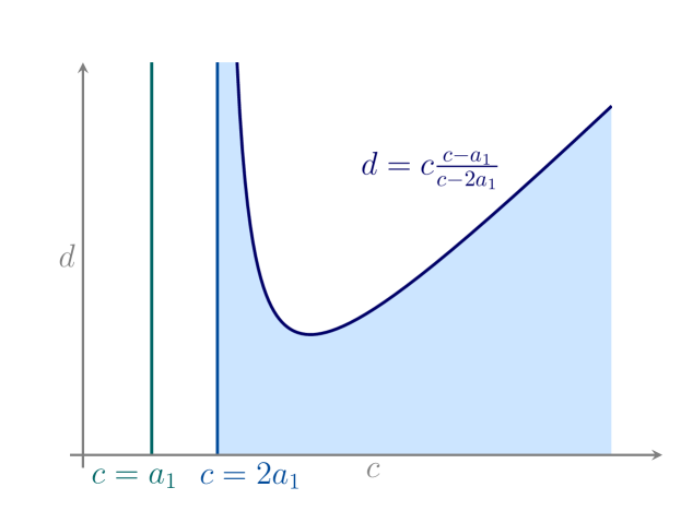
Figure 2: Constraints on the prefactors. We assume that $a_{1}$ is given.

Remarks:

1. If we investigate the first equation of the generic ODE System (1a) we can identify a relation satisfied by the non-trivial equilibrium $q_{ce},q_{re}$ which holds for any admissible set of parameters. If the condensation term in the original formulation is slightly extended to obtain the final equation

   $$\derivative{q_{c}}{t}=cq_{c}^{\gamma}-a_{1}q_{c}^{\gamma}-a_{2}q_{c}^{\beta_{c}}q_{r}^{\beta_{r}},$$ (50)

   i.e. the condensation and the autoconversion term have the same exponential behaviour, then we detect the following identity for the nontrivial steady states satisfying $\derivative{q_{c}}{t}=0$

   $$\frac{c-a_{1}}{a_{2}}=q_{ce}^{\beta_{c}-\gamma}q_{re}^{\beta_{r}}.$$ (51)

   This means that a certain combination of $q_{ce}$ and $q_{re}$ is constant in the set of the admissible exponents $\beta_{c},\beta_{r}$ and $\gamma$, provided the prefactors $a_{1},a_{2}$ and $c$ are held constant. Therefore, the value $\frac{c-a_{1}}{a_{2}}$ will be denoted as a conserved quantity in the sequel. Note that the validity of the identity (51) is unaffected by the inclusion of a term $B$ in (1b).

2. In case of $\gamma=1$, we obtain for the conserved quantity in equation (51) the term

   $$\frac{c-a_{1}}{a_{2}}=q_{c}^{\beta_{c}-1}q_{r}^{\beta_{r}}.$$ (52)

   This leads to a strong simplification of the first column in the Jacobi matrix $Df$, since with relation (52) the dependence on $q_{ce},q_{re}$ can be eliminated easily ($a_{11}=\quantity(1-\beta_{c})\quantity(c-a_{1})$, $a_{21}=a_{1}+\beta_{c}(c-a_{1})$). This property holds for all values of $\beta_{r}>0$.

3. Including the rain flux from above $B$ into equation (38b) leads to the modification

   $$\derivative{q_{r}}{t}=a_{1}q_{c}+a_{2}q_{c}^{\beta}q_{r}^{\beta}+B-dq_{r}.$$ (53)

   Thus, the determination of the non-trivial stationary point becomes more complicated. For the special case $\beta=2$ we investigate (53) explicitely. The stationary points shall be computed. Following the strategy at the beginning of the section, we add the two ODE equations (44a) and (53), which were set to zero before. This leads to the problem of finding real roots of the general cubic polynomial

   $$p_{3}(q_{re})=dq_{re}^{3}-Bq_{re}^{2}-c\frac{c-a_{1}}{a_{2}}.$$ (54)

   Using Cardano’s formulas (see, e.g., [Bosch, S. (2018)], chapter 6), we can determine the roots of the polynomial directly using the following terms:

   $$p = -\frac{1}{3}\quantity(\frac{B}{d})^{2}$$ (55)

   $$q = -\frac{2B^{3}+27d^{3}c\frac{c-a_{1}}{a_{2}}}{27d^{3}}$$ (56)

   $$\Delta = \quantity(\frac{q}{2})^{2}+\quantity(\frac{p}{3})^{3}=\frac{27d^{2}c^{2}\frac{\quantity(c-a_{1})^{2}}{a_{2}^{2}}-4B^{3}c\frac{c-a_{1}}{a_{2}}}{108d^{4}}$$ (57)

   whereas the parameter $\Delta$ decides about the quality of the roots (e.g. one real root and two complex conjugates for $\Delta>0$). One real root is given by

   $$u=\sqrt[3]{-\frac{q}{2}+\sqrt{\Delta}}, v=\sqrt[3]{-\frac{q}{2}-\sqrt{\Delta}}, q_{re}=u+v+\frac{B}{3d}.$$ (58)

   Since the sign of parameter $\Delta$ decides about the number of real roots, there is in general a bifurcation at $B_{1}$, which can be calculated using equation (57):

   $$27d^{2}c^{2}\frac{\quantity(c-a_{1})^{2}}{a_{2}^{2}}=4B_{1}^{3}c\frac{c-a_{1}}{a_{2}}\Leftrightarrow B_{1}=\sqrt[3]{\frac{27}{4}d^{2}\frac{c(c-a_{1})}{a_{2}}}.$$ (59)

   However, the condition (21) for the existence of a Turing instability might be violated at different values of $B$ as can be seen in the numerical simulations in the next section. The equilibrium states can be inserted into the Jacobi matrix for determining the eigenvalues. Using the relation (52), we see that the entries $a_{11}$ and $a_{21}$ do not depend on $B$. Therefore when the impact of $B$ on the existence of Turing instabilities shall be investigated, we only have to consider the entries $a_{12}(B),a_{22}(B)$. The sign of $a_{22}(B)$ is again the key parameter, and depends on the rain flux $B$. Actually, for a certain setting of parameters $c,a_{1},a_{2},d$ we will determine the qualitative behaviour and the possibility of Turing instabilities numerically (see next section).

4. The choice of exponents $\beta_{c}>1,\beta_{r}>1$ in the accretion term is motivated by existing models as e.g. the operational weather forecasting model IFS ([IFS DOCUMENTATION]), which contains such exponents. However, since the representation of collision processes in bulk models is not well-defined from a basic theory, there is actually no restriction of the choice of parameters. It is conceivable that the parameters also vary for different environmental regimes.

5. A nonlinear autoconversion generally affects the nontrivial stationary point as well as the entries $a_{12},a_{21}$ of the Jacobian. However, an analytical derivation of general conditions for the occurrence of Turing instabilities appears at least cumbersome through the nonlinear equation for the equilibrium, i.e.

   $$d-a_{1}\quantity(\frac{d}{c})^{\gamma}q_{r}^{\gamma-1}-a_{2}\quantity(\frac{d}{c})^{\beta}q_{r}^{2\beta-1}=0,\leavevmode\nobreak\ \leavevmode\nobreak\ \beta>1,\gamma>1.$$ (60)

   Numerical studies for different values of parameters $\beta,\gamma$ indicate that pattern formation is not restricted to the case $\gamma=1$. We could detect patterns in two simulations where $\beta_{c}=\beta_{r}=1.25$ and $\gamma=2$ or $\gamma=3$. The other parameters were chosen as in the 1D test case in the next section. The arising patterns are very similar to the patterns illustrated in the next section. This observation suggests that patterns can also evolve when the parameterisation of the autoconversion process is nonlinear. However, for an accretion term of the form $A_{2}=a_{2}q_{c}q_{r}$ one can show that even for exponents $\gamma>1$ these schemes do not allow Turing instabilities.

7 Numerical simulations of cloud pattern

Setup: We carry out 1D and 2D numerical simulations for investigating the special case ($\beta=2$) of the general cloud model allowing Turing instabilities, discussed in section 6. A pseudo-spectral method is applied for the numerical solution of the system, see appendix B. We choose a domain length of $L=50$ for the 1D case and a quadratic domain with length of $L=50$ for the 2D case, respectively. In both cases, the domain is cyclic as assumed in the linear stability analysis above. For the 1D simulations, we specify the parameters as follows:
$a_{1}=1,a_{2}=1,c=5,d=0.1,D_{1}=10^{3}$ and $D_{2}=10^{-1}$. In this scenario, the non-trivial stationary point is asymptotically stable and the parabola $p_{2}$ defined by equation (19) is negative for wave numbers $q^{2}=\frac{4\pi^{2}}{L^{2}}n^{2}$ with $n\in\{2,\dots,7\}$. Therefore, these modes give rise for linear instability and thus lead to Turing instability. For the 2D simulations we choose $d=0.13,D_{1}=10^{2},D_{2}=2.5\cdot 10^{-2}$. The other parameters are like in the 1D case. This slight modification does not change the qualitative behaviour. As initial condition for both cases we prescribe the equilibrium of the ODE system with spatial, normally distributed perturbations with amplitude of order $0.01$. In a first step, the system (44) is simulated, i.e. there is no rain flux from above ($B=0$). In a second step we will discuss the impact of the rain flux on the pattern formation in the simulations.

Results of 1D simulations without rain flux ($B=0$): First, we investigate the numerical simulations in one spatial dimension. In figure 3 the time evolution of the two variables $q_{c}$ (left panel) and $q_{r}$ (right panel) is shown. The horizontal axis represents the spatial extension of the 1D domain (with cyclic boundary conditions), the vertical axis represents time. The values of the cloud variables are represented by the colour code. Note, that we always consider dimensionless variables $q_{c},q_{r}$, thus the absolute values of these variables have no specific physical meaning.

The time evolution clearly shows the formation of spatial structures at times $t>200$ (in dimensionless time).

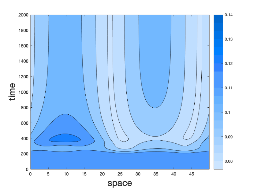
(a) $q_{c}$

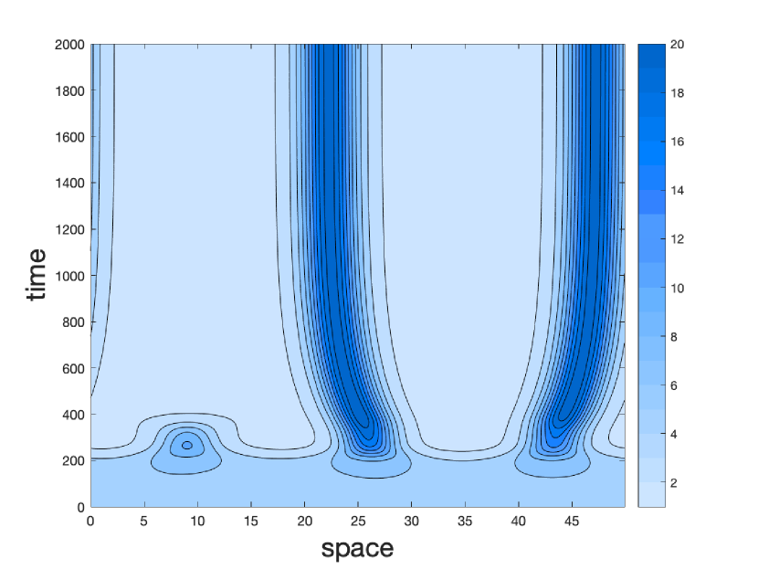
(b) $q_{r}$

Figure 3: Time evolution of the variables $q_{c}$ (left panel a) and $q_{r}$ (right panel b) in 1D. The spatial dimension is displayed on the horizontal axis (cyclic domain of length $L=50$).The time is displayed on the vertical axis. At $t\sim 200$ spatial structures form, which finally lead to a kind of wavy pattern at the end of the simulation

The spatial structure is forming out of the noise, i.e. the destabilised modes suddenly grow to larger sizes until they are saturated (and thus stopped) by the nonlinear terms. Their spatial distribution slightly changes during time until at around $t\sim 1200$ the situation is consolidated, i.e. the pattern stays quite stationary. In figure 4 the simulations at times $t=20/200/2000$ are shown. Here, the evolution can be seen clearly as well as the final “wavy” structure at $t=2000$. Note, that the variables $q_{c}$ and $q_{r}$ have contrary behaviour: for high values of $q_{c}$ the rain variable $q_{r}$ is quite small and vice versa. This can be explained by the collision terms, which act as in a generalised predator-prey system. If the predator population (i.e. the rain) is small, the cloud water survives and grows to larger values due to condensation only, since autoconversion is weak. If the rain becomes larger, it reduces the prey (the cloud water) due to collisions.

Using Fourier analysis (not shown) we see that only a part of the Fourier spectrum has reasonable amplitudes, whereas higher modes are of very low amplitudes. However, we do not see the distinct spectrum as predicted by linear stability theory. The reason for this is the nonlinear interaction of the different modes, which leads to non-vanishing amplitudes of modes which are stable according to the linear stability analysis. Nevertheless, we see that only a small part of the Fourier spectrum is present in the simulations.

Results of 2D simulations without rain flux ($B=0$): In a second simulation we use the 2D setup with white noise as before to investigate pattern formation in a 2D domain.

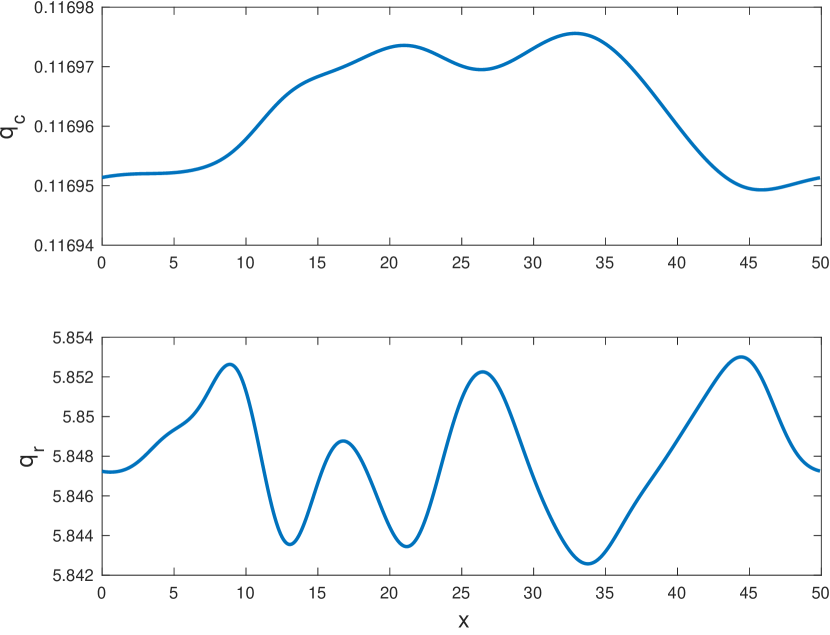
(a) $t=20$

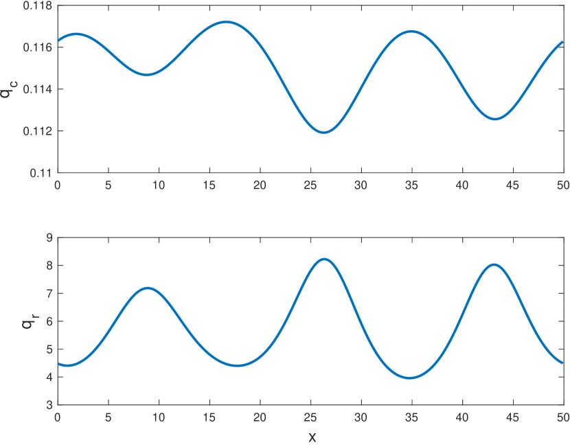
(b) $t=200$

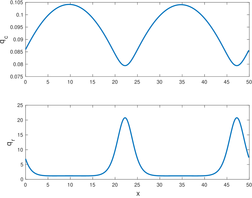
(c) $t=2000$

Figure 4: Spatial variation of the variables $q_{c}$ (top row) and $q_{r}$ (bottom row) for times $t=20$ (left), $t=200$ (middle), and $t=2000$ (right), respectively. Note the different scaling of the vertical axes. Actually, at $t=20$ there is almost no variation of $q_{c},q_{r}$ visible, whereas at $t=2000$ the change in $q_{c},q_{r}$ is obvious.

Qualitatively, we see the same behaviour for the 2D simulations of a quadratic domain of length $L=50$ with cyclic boundary conditions. After a short time, the simulation leads to growing unstable modes, which are then saturated by nonlinear terms in the model; these modes form spatial structures, which change only slightly over time until they stay stationary. Thus, pattern formation due to Turing instabilities can be observed as expected from theory. The structures in cloud water $q_{c}$ are less pronounced than in the rain water $q_{r}$. Nevertheless, the spatial patterns remain stationary, even for longer times.

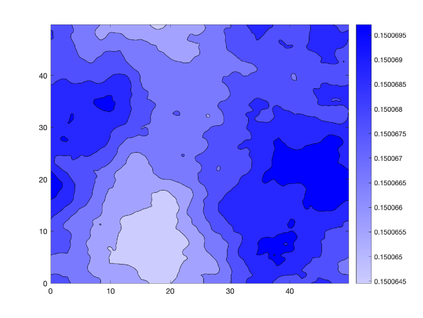
(a) $t=1$

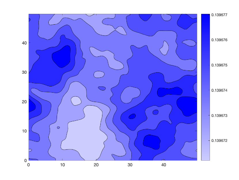
(b) $t=10$

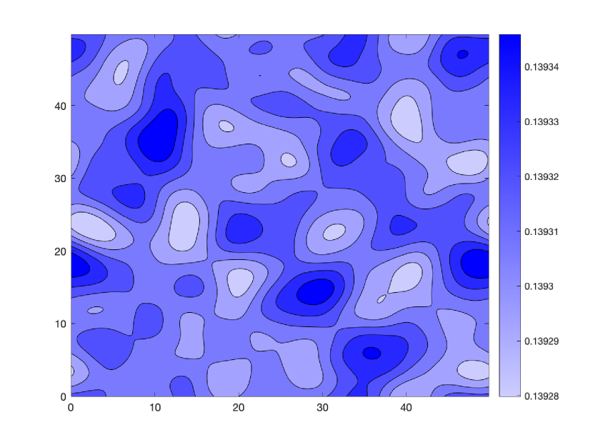
(c) $t=60$

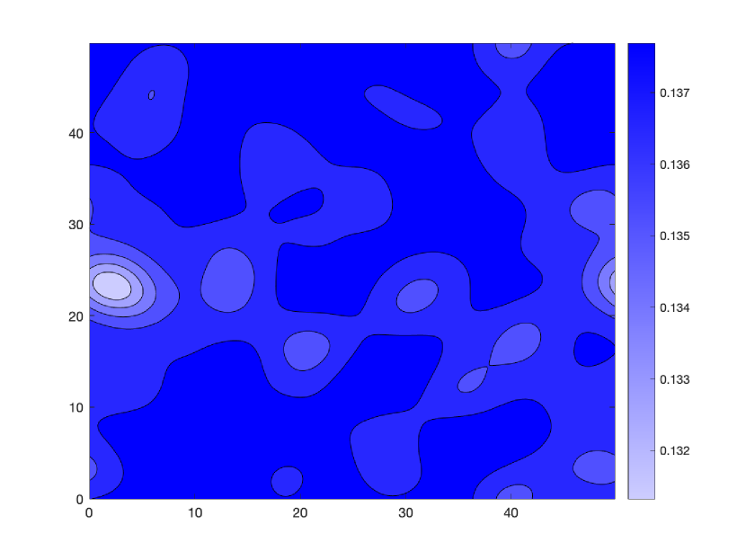
(d) $t=120$

Figure 5: Spatial distribution of cloud water $q_{c}$ in 2D for different simulation times ($t=1/10/60/120$). Note, that the pattern is already forming at times $t\sim 10$. For longer times, the pattern stays stationary although the absolute variation of the cloud water variable is very small over the whole 2D domain.

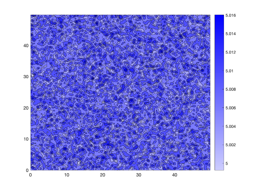
(a) $t=1$

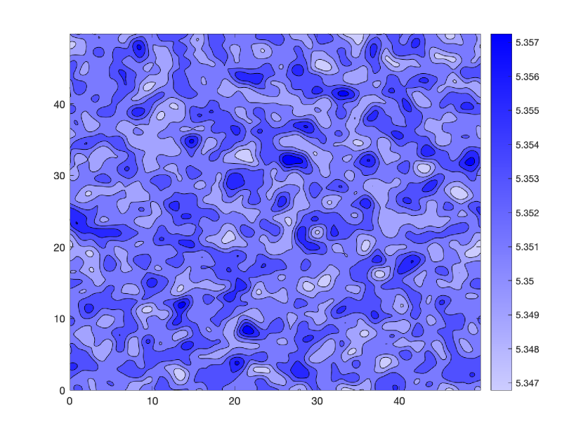
(b) $t=10$

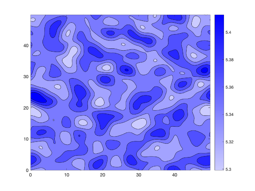
(c) $t=60$

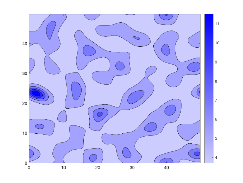
(d) $t=120$

Figure 6: Spatial distribution of rain water $q_{r}$ in 2D for different simulation times ($t=1/10/60/120$). The spatial structure for this variable is more pronounced than for the cloud water, i.e. the spatial variation of $q_{r}$ is quite large.

Results of 1D simulations for including the rain flux ($B>0$): In a last series of simulations we investigate the impact of the rain flux $B$, which was set to zero in section 6 for simplification of the analysis. Using the fixed parameters $c,a_{1},a_{2},d$ we can calculate the roots of the cubic polynomial determining the stationary points. One real root can be calculated as $q_{re}=u+v+\frac{B}{3d}$, see (58). The bifurcation value can be calculated as $B_{1}\sim 1.10521$. Actually, we additionally find that the eigenvalues $\sigma_{i}$ (for $i=1,2$) always have negative real part for $0<B<B_{1}$. Thus, the nontrivial stationary point is always asymptotically stable for rain flux from above in the relevant parameter range.

As described in section 6, the entries $a_{11}<0,a_{21}>0$ of the Jacobi matrix are constant, the entries $a_{12}(B),a_{22}(B)$ depend on the rain flux. For fulfilling the criterion for Turing instabilities (21), the sign of entry $a_{22}$ decides about the existence or non-existence of instabilities. For values $B<B_{2}\sim 0.137$ we obtain $a_{22}(B)>0$ (i.e. Turing instability is possible), whereas for $B>B_{2}$ the entry is negative.

We confirm these findings with a series of numerical simulations using different values $0<B<0.17$ for the set of parameters as specified at the beginning of the section. As predicted, for values $B<0.137$ we find Turing instabilities, whereas for $B>0.137$ there are no Turing instabilities. In Figure 7 the simulations at time $t=2000$ (i.e. steady state) depending on the parameter $B$ are shown. The absolute values of the pattern in $q_{c}$ and $q_{r}$ slightly vary with changing $B$; however, the quality of the pattern remains the same until values $B\sim B_{2}$ are reached. Passing this values, a homogeneous state in both variables can be seen and no pattern formation occurs. Note, that the boundary $B_{2}$ is not sharp, since the occurrence of the Turing instability depends also on the values of $D_{1},D_{2}$. Due to the large ratio of these coefficients, the transition in the simulations is very close to $B_{2}$.

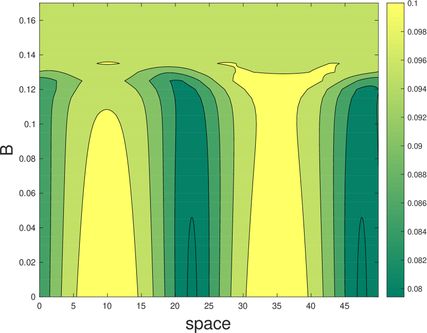
(a) $q_{c}$

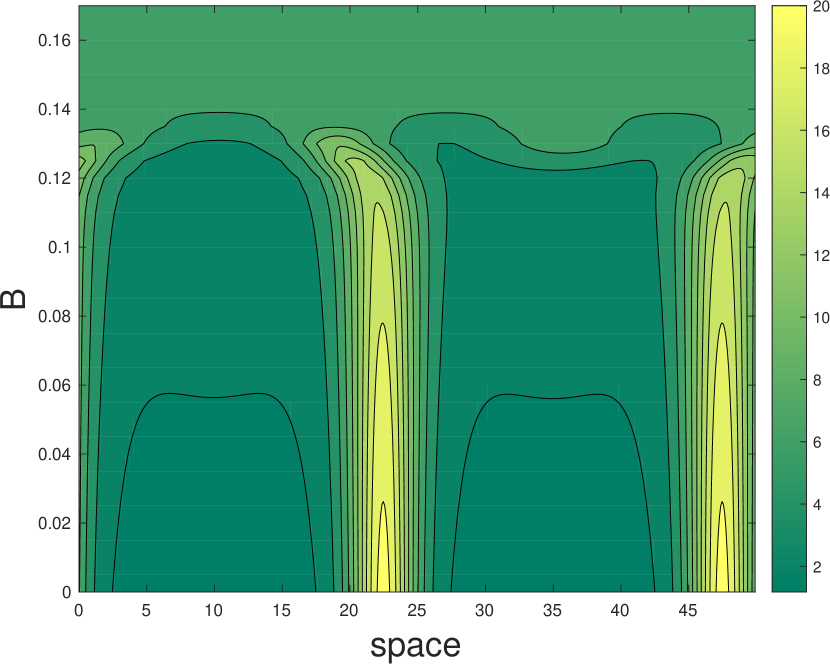
(b) $q_{r}$

Figure 7: The cloud variables $q_{c}$ (left panel a) and $q_{r}$ (right panel b) after 2000 time units for different values of the rain flux $B$ in 1D simulations. The x-axis displays the spatial direction, the y-axis represent different values of the rain flux $B$. The values of the cloud variables are given by the colour code.

8 Summary and conclusion

In this study we investigate a generic cloud model for pure liquid clouds on the possibility of Turing instabilities for forming spatial patterns. This kind of investigation is carried out for the first time for cloud pattern formation. For the theoretical and numerical investigations, the generic cloud model formulated in the former study [Rosemeier, J. et al. (2018)] is extended by diffusion terms, consisting of Laplacians in spatial directions. The model is analysed using stability theory for the linearisation around the steady states of the underlying two-dimensional ODE system. Analytical conditions for the existence of Turing instabilities can be determined. Since the model contains quite complex nonlinear terms with several parameters determining the overall quality of the steady states, it is very hard to find general conditions for the existence of Turing instabilities. However, the generic model always admits a trivial stationary point in terms of “no clouds, just rain falling through the layer”. This stationary point could be either stable or unstable, depending on the set of parameters. However, even in the stable case, the steady state cannot be destabilised by diffusion; thus, this state does not admit Turing instabilities. In addition, we can specify a class of models, which do not allow Turing instabilities at all. This class is characterised by a linear autoconversion term $A_{1}=a_{1}q_{c}$ and also a linear contribution of cloud water $q_{c}$ in the accretion term $A_{2}$. Well-known cloud models such as the standard COSMO cloud scheme ([Doms, G. et al. (2011)]) or the research model by [Wacker, U. (1992)] belong to this class. However, we can also provide a general class of cloud models, which allow Turing instabilities. If the exponents in the accretion parameterisation are chosen to be larger than 1 (i.e. $\beta=\beta_{c}=\beta_{r}>1$), the model can allow Turing instabilities and thus pattern formation. These theoretical findings could be confirmed by numerical simulations in one and two spatial dimensions. The inclusion of rain flux from above turns out to be an additional restriction for the instabilities. This is investigated for the special case $\beta=2$. If the rain flux becomes too large (i.e. if it surpasses a certain threshold $B>B_{2}$), the criterion for the existence of Turing instabilities is violated, as can be seen also in a series of 1D numerical simulations. This observation leads to the interpretation that collision processes in combination with the sedimentation of cloud particles play the major role for pattern formation; only if these processes can interact in a proper nonlinear way, Turing instabilities are possible. A strong rain flux from above can prevent the formation of cloud patterns; this might be explained by stronger collision terms, which finally almost extinct the cloud droplet population, thus diffusion can not counteract this process.

We can conclude that the generic cloud model admits Turing instabilities in special cases. However, several standard cloud models used in research and operational weather forecasts do not admit pattern formation due to Turing instabilities. It is still unknown how patterns in clouds form, especially, which processes lead to the emergence of cloud structures. The use of diffusion terms is motivated by the parameterisation of subgrid scale processes; this approach might be too simplistic for representing the underlying processes in a meaningful way. On the other hand, it is conceivable that pattern formation in clouds is dominated by Turing instabilities; in this case it might be a major drawback to use cloud models, which do not allow this type of pattern formation. Since pattern formation in clouds is far away from being understood, this observation has to be taken into account, and it might have an impact on the choice of cloud models for further investigations. For the investigation of cloud patterns, more theoretical studies are needed for a better understanding of the underlying processes and their interaction, which leads to the emergence of cloud structures.

Acknowledgement: We thank Maria Lukacova and Manuel Baumgartner for fruitful discussions. We acknowledges support of the Transregional Collaborative Research Center SFB/TRR 165 “Waves to Weather”, funded by the “Deutsche Forschungsgemeinschaft” (DFG), within the sub-project “Structure Formation on Cloud Scale and Impact on Larger Scales” (Project A2).

Appendix A Jacobian of ODE system (1)

The Jacobian $Df$ of the generic cloud model (without diffusion) can be calculated as

$$Df=\begin{pmatrix}c-\gamma a_{1}q_{c}^{\gamma-1}-a_{2}\beta_{c}q_{c}^{\beta_{c}-1}q_{r}^{\beta_{r}}&-a_{2}\beta_{r}q_{c}^{\beta_{c}}q_{r}^{\beta_{r}-1}\\ a_{1}\gamma q_{c}^{\gamma-1}+a_{2}\beta_{c}q_{c}^{\beta_{c}-1}q_{r}^{\beta_{r}}&a_{2}\beta_{r}q_{c}^{\beta_{c}}q_{r}^{\beta_{r}-1}-d\zeta q_{r}^{\zeta-1}\\ \end{pmatrix}.$$ (61)

In case of the trivial equilibrium state $q_{ce}=0,\leavevmode\nobreak\ q_{re}=\left(\frac{B}{d}\right)^{\frac{1}{\zeta}}$ the Jacobian reduces to

$$\begin{pmatrix}a_{11}&0\\ a_{21}&-d\zeta\left(\frac{B}{d}\right)^{\frac{\zeta-1}{\zeta}}\end{pmatrix}$$ (62)

Remember, that the Jacobian of the trivial state is only defined for values $\gamma\geq 1$, $\beta_{c}\geq 1$; otherwise the partial derivatives with respect to $q_{c}$ do not exist and the initial value problem is potentially not uniquely solvable, since the right hand side of the ODE system (1) is not Lipschitz continuous. For the entries in the matrix (62), we have to discriminate between different cases. First, we determine the value of $a_{11}$.

• For $\gamma=1,\beta_{c}=1$ we obtain $a_{11}=c-a_{1}-a_{2}\quantity(\frac{B}{d})^{\frac{\beta_{r}}{\zeta}}$. In this case, the trivial stationary point can be stable ($c<a_{1}+a_{2}\quantity(\frac{B}{d})^{\frac{\beta_{r}}{\zeta}}$) or unstable ($c>a_{1}+a_{2}\quantity(\frac{B}{d})^{\frac{\beta_{r}}{\zeta}}$).

• For $\gamma=1,\beta_{c}>1$ we obtain $a_{11}=c-a_{1}$. In this case, the trivial stationary point can be stable ($c<a_{1}$) or unstable ($c>a_{1}$).

• For $\gamma>1,\beta_{c}=1$ we obtain $a_{11}=c-a_{2}\quantity(\frac{B}{d})^{\frac{\beta_{r}}{\zeta}}$. In this case, the trivial stationary point can be stable ($c<a_{2}\quantity(\frac{B}{d})^{\frac{\beta_{r}}{\zeta}}$) or unstable ($c>a_{2}\quantity(\frac{B}{d})^{\frac{\beta_{r}}{\zeta}}$).

• For $\gamma>1,\beta_{c}>1$ we obtain $a_{11}=c$. In this case, the trivial stationary point is always unstable.

Second, the entry $a_{21}$ is investigated.

• For $\gamma=1,\beta_{c}=1$ we obtain $a_{21}=a_{1}+a_{2}\left(\frac{B}{d}\right)^{\frac{\beta_{r}}{\zeta}}$.

• For $\gamma=1,\beta_{c}>1$ we obtain $a_{21}=a_{1}$.

• For $\gamma>1,\beta_{c}=1$ we obtain $a_{21}=a_{2}\left(\frac{B}{d}\right)^{\frac{\beta_{r}}{\zeta}}$.

• For $\gamma>1,\beta_{c}>1$ we obtain $a_{21}=0$.

In any case, the entry $a_{21}$ does not affect the stability of the trivial stationary point.

Appendix B Pseudo-spectral method

The pseudo-spectral method is applied to the following type of semilinear equations

$$\derivative{x}{t}=L\quantity(x)+R\quantity(x).$$ (63)

where $L$ is a linear operator and $R$ a nonlinear operator. The model equation (2) represents such a system, the linear operator $L$ and the reaction term $R$ admit the form

$$L\quantity(q_{c},q_{r})=\left(\begin{array}[]{c}\quantity(c+D_{1}\laplacian)q_{c}\\ D_{2}\laplacian q_{r}\end{array}\right)$$ (64)

and

$$R\quantity(q_{c},q_{r})=\left(\begin{array}[]{c}-a_{1}q_{c}^{\gamma}-a_{2}q_{c}^{\beta_{c}}q_{r}^{\beta_{r}}\\ a_{1}q_{c}^{\gamma}+a_{2}q_{c}^{\beta_{c}}q_{r}^{\beta_{r}}-dq_{r}^{\zeta}+B\end{array}\right).$$ (65)

For the spatial discretisation a Fourier expansion is applied

$$y\quantity(t,x)=\sum_{n}\varphi\quantity(t)\exp(ik_{n}x).$$ (66)

Thus we obtain a system of ordinary differential equations

$$\derivative{\varphi_{n}}{t}\quantity(t)=l_{n}\varphi_{n}\quantity(t)+R_{n}\quantity(t),\qquad n=-\frac{N}{2},\dots,\frac{N}{2},$$ (67)

where $l_{n}$ is the matrix

$$l_{n}=\left(\begin{array}[]{rr}c-D_{1}k_{n}^{2}&0\\ 0&-D_{2}k_{n}^{2}\\ \end{array}\right).$$ (68)

The nonlinear operator $R$ can be expressed with Fourier modes

$$R\quantity(q_{c}\quantity(t),q_{r}\quantity(t))\approx\sum_{n=-\frac{N}{2}}^{\frac{N}{2}}R_{n}\quantity(t)\exp(ik_{n}x).$$ (69)

Therefore, the formulation of equation (67) requires a Fourier transform. In addition after each time step the solution in the Fourier space, given through (67), can be transformed back and the reaction term can be computed for that time step. The transformations can be done with a Fast Fourier Transform.

The system (67) can be solved with the exponential integrator scheme ([Hochbruck, M. and Ostermann, A. (2010)]) of second order (ETD2 scheme). The ETD2 scheme is a two step method. The first step can be computed with the exponential integrator scheme of first order (ETD1 scheme).

References

- [Beheng, K. D. (2010)] Beheng, Klaus D. (2010). The Evolution of Raindrop Spectra: A Review of Microphysical Essentials. In: Rainfall: State of the Science. American Geophysical Union, S. 29–48.
- [Bodenschatz, E. et al. (2000)] Bodenschatz, E., Pesch, W and Ahlers, G (2000). Recent developments in Rayleigh-Benard convection. In: Annual Review of Fluid Mechanics. 32, S. 709–778.
- [Bosch, S. (2018)] Bosch, S. (2018). Algebra - From the Viewpoint of Galois Theory. Springer, 367 pp.
- [Cross, M. and Greenside, H. (2009)] Cross, M. and Greenside, H. (2009). Pattern Formation and Dynamics in Nonequilibrium Systems. Cambridge University Press.
- [Cross, M. C., Hohenberg, P. C. (1993)] Cross, Mark C and Hohenberg, Pierre C (1993). Pattern formation outside of equilibrium In: Reviews of Modern Physics. 65, S. 851.
- [Deardorff, J. W. (1972)] Deardorff, JW (1972). Numerical Investigation of Neutral and Unstable Planetary Boundary-Layers In: Journal of the Atmospheric Sciences 29.1, S. 91–115.
- [Doms, G. et al. (2011)] Doms, G., Förstner, J., Heise, E., Herzog, H.-J., Mironow, D., Raschendorfer, M., Reinhardt, T., Ritter, B., Schrodin, R., Schulz, J.-P. and Vogel, G. (2011). A Description of the Nonhydrostatic Regional COSMO Model. Part II: Physical Parameterization.
- [IFS DOCUMENTATION] ECMWF (2017). IFS DOCUMENTATION – Cy43r3. Part IV: Physical Processes.
- [Etling, D. and Brown, R. (1993)] Etling, D. and Brown, R. (Aug. 1993). Roll Vortices in the Planetary Boundary-Layer - A Review. In: Boundary-Layer Meteorology 65.3, pp. 215–248.
- [Glassmeier, F. and Feingold, G. (2017)] Glassmeier, Franziska and Feingold, Graham (2017). Network approach to patterns in stratocumulus clouds In: Proceedings of the National Academy of Sciences of the United States of America 114.40, S. 10578–10583.
- [Hanke, M, and Porz, N. (2020)] Hanke, Martin and Porz, Nikolas (2020). Unique Solvability of a System of Ordinary Differential Equations Modeling a Warm Cloud Parcel In: SIAM Journal on Applied Mathematics 80.2, S. 706–724.
- [Hochbruck, M. and Ostermann, A. (2010)] Hochbruck, M. and Ostermann, A. (2010). Exponential integrators. In: Acta Numerica 19, pp. 209–286.
- [Kessler, E. (1969)] Kessler, Edwin (1969). On the Distribution and Continuity of Water Substance in Atmospheric Circulations In: On the Distribution and Continuity of Water Substance in Atmospheric Circulations. Boston, MA: American Meteorological Society, S. 1–84.
- [Khain, A. P. et al. (2015)] Khain, A. P., Beheng, K. D., Heymsfield, A., Korolev, A., Krichak, S. O., Levin, Z., Pinsky, M., Phillips, V., Prabhakaran, T., Teller, A., Heever, S. C. van den and Yano, J. -I. (2015). Representation of micro- physical processes in cloud-resolving models: Spectral (bin) microphysics versus bulk parameterization. In: Reviews of Geophysics 53.2, S. 247–322.
- [Khairoutdinov, M. and Kogan, Y. (2000)] Khairoutdinov, M. and Kogan, Y. (2000). A New Cloud Physics Parameterization in a Large-Eddy Simulation Model of Marine Stratocumulus. In: Monthly Weather Review 128.1, pp. 229–243.
- [Khouider, B. and Bihlo, A. (2019)] Khouider, Boualem and Bihlo, Alexander (2019). A New Stochastic Model for the Boundary Layer Clouds and Stratocumulus Phase Transition Regimes: Open Cells, Closed Cells, and Convective Rolls. In: Journal of Geophysical Research-Atmospheres 124.1, S. 367–386.
- [Köhler, H. (1936)] Köhler, H. (1936). The nucleus in and the growth of hygroscopic droplets. In: Transactions of the Faraday Society 32, S. 1152–1161.
- [Kondepudi, D. and Prigogine, I. (2015)] Kondepudi, D. and Prigogine, I. (2015). Modern Thermodynamics. Wiley.
- [Korolev, A.V. and Mazin, I.P. (2003)] Korolev, AV and Mazin, IP (2003). Supersaturation of water vapor in clouds. In: Journal of the Atmospheric Sciences 60.24, S. 2957–2974.
- [Lee, J. et al. (1994)] Lee, J., Chou, J., Weger, R., and Welch, R. (July 1994). Clustering, randomness, and regularity in cloud fields .4. Stratocumulus Cloud Fields. In: Journal of Geophysical Research-Atmospheres 99.D7, pp. 14461–14480.
- [Monroy, D. L. and Naumis, G. G. (2020)] Monroy, Diana L. and Naumis, Gerardo G. (2020). Description of mesoscale pattern formation in shallow convective cloud fields by using time-dependent Ginzburg-Landau and Swift-Hohenberg stochastic equations. arXiv:2006.03981.
- [Morrison, H. et al. (2020)] Morrison, Hugh, Lier-Walqui, Marcus van, Fridlind, Ann M., Grabowski, Wojciech W., Harrington, Jerry Y., Hoose, Corinna, Korolev, Alexei, Kumjian, Matthew R., Milbrandt, Jason A., Pawlowska, Hanna, Posselt, Derek J., Prat, Olivier P., Reimel, Karly J., Shima, Shin-Ichiro, Diedenhoven, Bastiaan van and Xue, Lulin (2020). In: Journal of Advances in Modeling Earth Systems 12.8, e2019MS001689.
- [Murray, J. D. (2003)] Murray, J. D. (2003). Mathematical Biology II: Spatial Models and Biomedical Applications. 12.8, e2019MS001689.
- [Nair, U. et al. (1998)] Nair, U., Weger, R., Kuo, K., and Welch, R. (May 1998). Clustering, randomness, and regularity in cloud fields - 5. The nature of regular cumulus cloud fields. In: Journal of Geophysical Research-Atmospheres 103.D10, pp. 11363–11380.
- [Rosemeier, J. et al. (2018)] Rosemeier, Juliane, Baumgartner, Manuel and Spichtinger, Peter (2018). Intercomparison of warm-rain bulk microphysics schemes using asymptotics. In: Math. Clim. Weather Forecast. 4.1, S. 104–124.
- [Seifert, A. et al. (2014)] Seifert, A., Blahak, U. and Buhr, R. (2014). On the analytic approximation of bulk collision rates of non-spherical hydrometeors. In: Geoscientific Model Development 7.2, S. 463–478.
- [Seifert, A. and Beheng, K. D. (2006)] Seifert, Axel and Beheng, Klaus D. (2006). A two-moment cloud microphysics parameterization for mixed-phase clouds. Part 1: Model description. 92.1, S. 45–66.
- [Stull, R. B. (1988)] Stull, R. B. (1988). An Introduction to Boundary Layer Meteorology. Bd. 13. Atmospheric and Oceanographic Sciences Library. Springer, 688 pp.
- [Turing, A. M. (1952)] Turing, AM (1952). The Chemical Basis of Morphogenesis. In: Philosophical Transactions of the Royal Society of London Series B-Biological Sciences 237.641, S. 37–72.
- [Wacker, U. (1992)] Wacker, Ulrike (1992). Structural Stability in Cloud Physics Using Parameterized Microphysics. In: Beitr äge zur Physik der Atmosphäre 65.3, S. 231–242.
- [Weger, R. et al (1993)] Weger, R., Lee, J., and Welch, R. (Oct. 1993). Clustering, randomness, and regularity in cloud fields .3. The Nature and Distribution of Clusters. In: Journal of Geophysical Research-Atmospheres 98.D10, pp. 18449–18463.
- [Weger, R. et al (1992)] Weger, R., Lee, J., Zhu, T., and Welch, R. (Dec. 1992). Clustering, randomness, and regularity in cloud fields. 1. Theoretical Considerations. In: Journal of Geophysical Research-Atmospheres 97.D18, pp. 20519–20536.
- [Zhu et al (1992)] Zhu, T., Lee, J., Weger, R., and Welch, R. (Dec. 1992). Clustering, randomness, and reg- ularity in cloud fields. 2. Cumulus Cloud Fields. In: Journal of Geophysical Research- Atmospheres 97.D18, pp. 20537–20558.