Orientational ordering in a fluid of hard kites: A density-functional-theory study

Abstract

Using Density Functional Theory we theoretically study the orientational properties of uniform phases of hard kites – two isosceles triangles joined by their common base. Two approximations are used: Scaled Particle Theory, and a new approach which better approximates third virial coefficients of two-dimensional hard particles. By varying some of their geometrical parameters kites can be transformed into squares, rhombuses, triangles, and also very elongated particles, even reaching the hard-needle limit. Thus a fluid of hard kites, depending on the particle shape, can stabilize isotropic, nematic, tetratic and triatic phases. Different phase diagrams are calculated, including those of rhombuses, and kites with two of their equal interior angles fixed to $90^{\circ}$, $60^{\circ}$ and $75^{\circ}$. Kites with one of their unequal angles fixed to $72^{\circ}$, which have been recently studied via Monte Carlo simulations, are also considered. We find that rhombuses and kites with two equal right angles and not too large anisometry stabilise the tetratic phase but the latter stabilize it to a much higher degree. By contrast, kites with two equal interior angles fixed to $60^{\circ}$ stabilize the triatic phase to some extent, although it is very sensitive to changes in particle geometry. Kites with the two equal interior angles fixed to $75^{\circ}$ have a phase diagram with both tetratic and triatic phases, but we show the nonexistence of a particle shape for which both phases are stable at different densities. Finally the success of the new theory in the description of orientational order in kites is shown by comparing with Monte Carlo simulations for the case where one of the unequal angles is fixed to $72^{\circ}$. These particles also present phase diagrams with stable tetratic and triatic phases.

I Introduction

The study of entropically-driven phase transitions in liquid crystals has been an active field of research from the pioneering work of Onsager onsager , having a major boost in the 80’s and 90’s frenkel ; veerman ; allen ; jackson ; bolhuis ; mulder and continuing as a very active topic of research up to the present kooij ; wensink ; cheng ; schiling ; cinacchi ; odriozola ; yang ; cuetos ; dijkstra2 ; dijkstra3 ; rafael . These works theoretically and experimentally showed that liquid-crystalline uniform phases, such as uniaxial or biaxial nematics (N), and non-uniform phases such as smectic and columnar phases, can be stabilized solely by extremely short-ranged repulsive particle interactions. Several statistical-mechanical models were developed for the description of thermodynamic and structural properties of hard-body fluids in which the Helmholtz free-energy has only an entropic contribution, with Density Functional Theory (DFT) being one of the most successful theoretical tool in this respect mederos .

Most theoretical works naturally concentrated on 3D systems since in experiments the ratios between the lengths of the samples along the three spatial directions and those of the particles are large enough to conform to the three-dimensional spatial criterion. However new experimental techniques have been recently developed for the synthesis of taylor-shaped hard-core interacting microparticles, which can now be studied under extreme confinement along one spatial direction chaikin ; zhao3 ; zhao5 . These systems can be thought of as single monolayers of particles subject to Brownian motion in two dimensions (2D).

Recent experimental works on these effectively 2D hard-body fluids showed the stability of exotic uniform liquid-crystalline phases such as tetratic (T) chaikin ; zhao3 , and triatic (TR) zhao5 . The symmetries of these phases can be rationalized from the properties of the orientational distribution function, $h(\phi)$, defined as the probability density for the angle $\phi$ between the particle axis and the nematic director. Four- or six-fold symmetries, i.e. $h(\phi)=h(\phi+2\pi/n)$, indicate the presence of T ($n=4$) or TR ($n=6$) phases, respectively. Theoretical studies using MC simulations frenkel1 ; donev and DFT schlacken ; MR3 ; MR4 predicted the stability of the T phase long before the experiments were conducted. By contrast, theoretical studies of the TR phase dijkstra ; MR2 appeared after the phase was discovered in experiments zhao5 .

Depending on their particular (usually polygonal) shape, 2D particles also crystallize into a variety of structures with different symmetries. These symmetries exhibit a subtle dependence on geometrical details such as the roundness of the particle corners. For example, in the case of regular polygons with more than seven sides, the crystal melts continuously into an hexatic phase and then transforms into an isotropic (I) fluid through a first order transition glotzer . Triangles, squares and hexagons exhibit a Kosterlitz-Thouless transition from I to TR, T and hexatic phases, respectively, which then crystallize glotzer . Finally, pentagons undergo a one-step first-order melting from crystal to I glotzer . However in a fluid of squares with rounded corners, the orientationally disordered hexatic-rotator, or orientationally-ordered rhombic crystalline phases are stabilized as density is increased zhao3 ; escobedo , but no T phase was found; instead, an hexatic phase between I and crystal appears for a certain roundness parameter escobedo . In the case of hexagons with rounded corners a transition occurs between an hexagonal rotator crystal and an hexagonal crystal zhao4 . DFT studies revealed that non-polygonal particles such as hard rectangles schlacken ; MR3 ; MR4 or superellipses close enough to the rectangular shape szabi can stabilize the T phase when the aspect ratio is below a certain critical value.

Some recent experimental works have shown the tendency of some achiral 2D particles, such as equilateral triangles or square crosses, to form chiral crystalline structures at high packing fractions zhao5 ; mayoral ; zhao6 . By mixing particles with exotic geometries, e.g. kites and darts, it is also possible to obtain quasi-periodic structures in which kite- and dart-shaped tiles form pentagonal stars, arranged in turn into different close-packed superstructural patterns zhao7 . In recent experiments the phase diagram of kites with one of its unequal interior angles, $\alpha_{1}$, fixed to $72^{\circ}$ with the other, $\alpha_{2}$ being variable, was elucidated zhao1 . Interestingly, kites with a shape departing from the square geometry also form a T phase for some values of $\alpha_{2}$ zhao1 .

In this work the phase behavior and orientational properties of a uniform fluid of hard kites is studied theoretically. DFT is used, based on two alternative approximations: the standard Scaled Particle Theory (SPT), and a new approach which better approximates the third virial coefficient. Different constraints on the interior angles $\alpha_{i}$ of kites are selected. The kite geometry has the square ($\alpha_{i}=90^{\circ}$) and equilateral triangle ($\alpha_{1}=60^{\circ}$, $\alpha_{2}=180^{\circ}$) as limiting cases. Actually, these shapes maximize T and TR stability, respectively. We are interested in changes in the stability of these phases resulting from distortions of these two polygonal geometries, always within the kite-like shape. Therefore, the following constraints on the interior angles are applied: (i) $\alpha_{1}=\alpha_{2}$ (rhombuses having the square as a limiting case), (ii) $\alpha_{1}+\alpha_{2}=180^{\circ}$ (kites with the same limiting case and with both equal interior angles fixed to $90^{\circ}$), (iii) $\alpha_{1}+\alpha_{2}=240^{\circ}$ (kites with the equilateral triangle as a limiting case), and (iv) $\alpha_{1}+\alpha_{2}=210^{\circ}$ (kites with the limiting case consisting of an isosceles triangle with opening angle equal to $30^{\circ}$). Phase diagrams of all these cases are calculated. By comparing the first and second cases we show that the latter has a larger stability region for the T phase, i.e. a larger interval for $\alpha_{1}$ where the phase is stable. Also, the TR phase of hard equilateral triangles is very sensitive to changes in particle geometry, resulting in the lowest $\alpha_{1}$-interval for which the phase is stable. The case (iv) is very interesting since the phase diagram presents stable T and TR phases for different $\alpha_{1}$. The existence of a particular particle shape (with fixed $\alpha_{i}$) that exhibits both phases at different densities can be discarded. Finally, we calculated the phase diagram of kites with one of the unequal angles, $\alpha_{1}$, fixed to $72^{\circ}$, while the other one, $\alpha_{2}$, is freely varied. This study allowed our new DFT theory to be contrasted with the recent Monte Carlo (MC) simulations of Ref. zhao1 . We showed that, by varying $\alpha_{1}$ in the interval $[54^{\circ},180^{\circ}]$, both phases, T and TR, are stable, with the former having the largest stability region. The size of this region is similar to that found in the simulations. This result, together with the agreement in the values of packing fractions at the I-T transition, gives support to the validity of our DFT approach.

II Theory

In this section we introduce the theoretical tools used to study the equilibrium properties of the fluid of hard kites. In Sec. II.1 the two version of DFT used are presented: the one based on the classical SPT, and a new one which better approximates three-body correlations in general systems of 2D hard convex particles. In Sec. II.2 the particle model used and the properties of the excluded area (the main ingredient of the DFTs) are considered. Finally Sec. II.3 presents a bifurcation analysis using both theories to calculate the I-(TR,T) bifurcation curves; when the SPT approximation is used analytic expressions can be obtained. The bifurcation analysis from the (T,TR) phases to the N phase is described in Sec. A.

II.1 DFT for 2D hard convex particles

The density expansion of the fluid pressure is based on the knowledge of the virial coefficients $B_{n}$. For hard spheres or hard disks these coefficients are known to high order. However for anisotropic hard bodies only the cases $n=2$ and $3$ are available in general, and the latter case is only known for a few geometries. In 2D the exact second-virial coefficient of convex bodies in the orientationally disordered I phase is given by kihara ; tarjus

$$B_{2}=a+\frac{{\cal L}^{2}}{4\pi}=a\left(1+\gamma\right),$$ (1)

with $a$ and ${\cal L}$ the area and perimeter of the particle. The anisometry parameter

$$\gamma=\frac{{\cal L}^{2}}{4\pi a},$$ (2)

is a measure of how much the particle geometry deviates from a disk. In this case $\gamma=1$, while for other convex particles $\gamma>1$.

A good approximation for the third virial coefficient, again for orientationally disordered particle configurations, is given by

$$B_{3}=a^{2}+\delta_{1}\frac{{\cal L}^{2}a}{4\pi}+\delta_{2}\frac{{\cal L}^{4}}{\left(4\pi\right)^{2}}=a^{2}\left(1+\delta_{1}\gamma+\delta_{2}\gamma^{2}\right),$$ (3)

where $\delta_{i}$ are numerical coefficients obtained by fitting the available values of $B_{3}$ (calculated from MC integration) for several convex particles boublik ; tarjus ; MR4 .

An interesting limit is the Onsager hard-needle limit, where particles become infinitely elongated. In this limit the particle aspect ratio $\kappa$ becomes infinite, $\kappa\to\infty$. The behavior of the ratio of $B_{3}$ to $B_{2}^{2}$ is onsager ; tarjus

$$\lim_{\kappa\to\infty}\frac{B_{3}}{B_{2}^{2}}=0,\ \text{in}\ \text{3D},$$ (4)

$$\lim_{\kappa\to\infty}\frac{B_{3}}{B_{2}^{2}}\simeq 0.514,\ \text{in}\ \text{2D}.$$ (5)

The 3D limit explains the success of DFT theories for 3D hard-body fluids based only on the exact second virial coefficient. By contrast, because of (5), the corresponding 2D theories have a lesser degree of accuracy and third and possibly higher-order virial coefficients are necessary in the theory to adequately account for particle correlations in the fluid.

For orientationally ordered phases, the anisometry parameter becomes a functional of the orientational distribution function $h(\phi)$:

$$\gamma[h] = \frac{\langle\langle A_{\rm spt}(\phi)\rangle\rangle_{h(\phi)}}{2a}$$ (6)

$$\equiv \frac{1}{2a}\int_{0}^{2\pi}d\phi_{1}\int_{0}^{2\pi}d\phi_{2}h(\phi_{1})h({\phi_{2}})A_{\rm spt}(\phi_{12}),$$

This is defined as a double angular average of $A_{\rm spt}(\phi)$, which is directly related to the excluded area between two particles as

$$A_{\rm spt}(\phi)\equiv A_{\rm excl}(\phi)-2a.$$ (7)

Note that, inserting the uniform distribution function $h(\phi)=(2\pi)^{-1}$ in (6), we obtain

$$\gamma=\frac{1}{4\pi a}\int_{0}^{2\pi}d\phi A_{\rm spt}(\phi)=\frac{{\cal L}^{2}}{4\pi a}.$$ (8)

The latter equality is proven in Refs. isihara ; kihara for general convex particles. Following a similar reasoning, an approximation for the third-virial coefficient of orientationally ordered phases can be obtained by substituting the value of the anisometry parameter by its functional form $\gamma\to\gamma[h]$ in (3).

For perfectly oriented nematic phase, with the symmetric orientational distribution function $h(\phi)=\left[\delta(\phi)+\delta(\phi-\pi)\right]/2$ ($\delta(x)$ being the Dirac-delta function), one obtains from Eq. (6) $\gamma[h]=\left[A_{\rm excl}(0)+A_{\rm excl}(\pi)\right]/(4a)-1$. Now taking into account that the excluded area of perfectly antiparallel oriented convex particles is equal to four times the particle area, $A_{\rm excl}(\pi)=4a$, we obtain $\gamma[h]=A_{\rm excl}(0)/(4a)$. Finally if particles are symmetric ($A_{\rm excl}(0)=A_{\rm excl}(\pi)$) the same value as for hard disks, $\gamma[h]=1$, is obtained.

Following the SPT approximation, the excess free-energy per particle in thermal units $kT=\beta^{-1}$ is given by

$$\varphi_{\rm exc}[h]\equiv\frac{\beta{\cal F}_{\rm exc}[h]}{N}=-\log\left(1-\eta\right)+\frac{\gamma[h]\eta}{1-\eta},$$ (9)

with $k$ the Boltzmann constant, $T$ the temperature and $N$ the total number of particles. ${\cal F}_{\rm exc}[h]$ is the Helmholtz free-energy density functional. The fluid packing fraction is $\eta=\rho a$ with $\rho$ the number density. Note that the density expansion of (9), up to second order, is

$$\varphi_{\rm exc}[h] \simeq a\left(1+\gamma[h]\right)\rho+\frac{1}{2}\left(1+2\gamma[h]\right)a^{2}\rho^{2}$$ (10)

$$= B_{2}[h]\rho+\frac{1}{2}B_{3}^{(\rm spt)}[h]\rho^{2}.$$

This gives the exact expression for the second virial coefficient given by (1), and an approximate value for the third one as

$$B_{3}^{(\rm spt)}[h]=\left(1+2\gamma[h]\right)a^{2}.$$ (11)

We note that the third virial coefficient for the I phase, as obtained from SPT, gives the incorrect hard-needle limit

$$\lim_{\kappa\to\infty}\frac{B_{3}^{(\rm spt)}}{B_{2}^{2}}=\lim_{\kappa\to\infty}\frac{1+2\gamma}{\left(1+\gamma\right)^{2}}=0,$$ (12)

since $\gamma\to\infty$ as $\kappa\to\infty$. Comparing Eqns. (3) and (11) we conclude that, for hard disks ($\gamma=1$), both expressions coincide if and only if $\delta_{1}+\delta_{2}=2$.

To overcome the failure of SPT to describe the correct scaling behavior in the Onsager limit, we here propose a different expression for the excess free-energy which gives the exact value of $B_{2}$ and the approximation (3) for $B_{3}$, resulting in the correct scaling for $\kappa\to\infty$. We also require to recover the SPT expression for hard disks, so we choose the condition $\delta_{1}+\delta_{2}=2$. Finally we set $\displaystyle{\delta_{2}=\frac{1}{2}}$ so that the hard-needle limit, $\displaystyle{\frac{B_{3}}{B_{2}^{2}}\to 0.514\approx\frac{1}{2}}$, is accurately approximated.

With these constraints in mind our proposal is

$$\varphi_{\rm exc}[h]=-\log(1-\eta)+\frac{\gamma[h]\eta}{1-\eta}$$

$$+\gamma[h]\left(\gamma[h]-1\right)\left(\frac{1}{2}+r\eta\right)\left(\frac{\eta}{1-\eta}+\log(1-\eta)\right),$$ (13)

where an extra term is included, proportional to $r\eta$, which only affects the expressions for the fourth and higher virial coefficients. The coefficient $r$ can be chosen to accurately describe the packing fraction of the I-T transition of the hard square fluid (as obtained from MC simulations).

The ideal part of the free-energy per particle, dropping the thermal area, is

$$\varphi_{\rm id}[h] \equiv \frac{\beta{\cal F}_{\rm id}[h]}{N}$$ (14)

$$= \log\eta-1+\int_{0}^{2\pi}d\phi h(\phi)\log\left(2\pi h(\phi)\right).$$

The scaled fluid pressure $\displaystyle{\beta pa=\eta^{2}\frac{\partial\varphi}{\partial\eta}}$ is calculated from the the total free-energy per particle $\varphi[h]=\varphi_{\rm id}[h]+\varphi_{\rm exc}[h]$ as

$$\beta pa = \frac{\eta}{1-\eta}+\frac{\gamma[h]\eta^{2}}{(1-\eta)^{2}}+\gamma[h]\left(\gamma[h]-1\right)\eta^{2}$$ (15)

$$\times \left[\left(\frac{1}{2}+r\right)\frac{\eta}{(1-\eta)^{2}}+r\log(1-\eta)\right].$$

As already mentioned the anisometry asymptotically behaves as $\gamma[h]\sim 1$ for very high orientational ordering. Thus, in the case $(\gamma[h]-1)/(1-\eta)^{2}\sim 0$, Eqns. (13) and (15) show that the SPT (the first two terms in both equations) is also recovered at high packing fractions.

In Sec. III we use the SPT approximation (9) and our new proposal (13) to calculate the phase diagrams of hard kites. As usual, the total free-energy per particle $\varphi[h]$ is minimised with respect to $h(\phi)$ to obtain its equilibrium value. The minimization is much less demanding numerically using truncated Fourier expansions for the orientational distribution function,

$$h(\phi)=\frac{1}{2\pi}\left(1+\sum_{k=1}^{n}h_{k}\cos(2k\phi)\right),$$ (16)

and then minimizing $\varphi[h]$ with respect to the Fourier coefficients $\{h_{k}\}$. The second order I-(T,TR) transition lines are calculated using a bifurcation analysis (see Sec. II.3), while the coexisting binodals are obtained from the equality of the chemical potentials $\displaystyle{\beta\mu=\varphi+\frac{\beta pa}{\eta}}$ and pressures $\beta pa$ (evaluated at the equilibrium values of $\{h_{k}\}$) in the two coexisting phases.

The only uniform orientationally ordered phase in a fluid of hard squares is the tetratic phase. From the excluded area between two hard squares we obtain $A_{\rm spt}(\phi)=2a\left(|\sin\phi|+|\cos\phi|\right)$ (the key quantity to calculate $\gamma[h]$). The symmetry of the T phase implies $h(\phi)=h(\phi+\pi/2)$, and consequently the Fourier expansion (16) should only contain even integers $k=2j$ ($j\geq 1$). $\varphi[h]$ is then minimised with respect to $\{h_{2j}\}$ for a given $\eta$, with $\varphi_{\rm ex}[h]$ given by SPT [Eq. (9)], and also using our new proposal [Eq. (13)] with $r=1$ and $2$. Inserting the equilibrium values into (15) and its SPT-version (the first two terms), three different approximations for the equations of state (EOS) are obtained. Results are shown in Fig. 1, which also includes the EOS of hard squares obtained from MC simulations, Ref. frenkel1 . The left arrow indicates the I-T transition from simulations, which occurs for $\eta\simeq 0.7$. The conclusion is that the choice $r=2$ predicts the transition much better, while the SPT gives a much higher value $\eta\approx 0.855$. The figure also shows how the theories overestimate the fluid pressure with respect to MC simulations, particularly close to the phase transition. It should be taken into account that simulation results also include the crystal phase at densities higher than $\eta\simeq 0.78$ (the right arrow in Fig. 1). However the crystal phase has not been included in our DFT study, so that it makes sense that both theories overestimate the pressure at high densities.

The SPT approximation had been extensively used in the description of the phase behavior of hard particle fluids. As will be shown in Sec. II.3, it has the advantage of producing analytic expressions of the packing fraction at the continuous transition from I to the orientationally ordered phases as a function of the particle characteristic lengths. Because of this we decided to calculate most phase diagrams with the SPT formalism. The new proposal (13) was numerically implemented to calculate two different phase diagrams with the aim to comparing both theories. Also we wanted to confront the new theory with recent MC simulations for hard kites zhao1 .

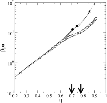
Figure 1: EOS of hard squares according to SPT (dotted), the new approach with $r=1$ (dashed) and with $r=2$ (solid). Open circles represent MC simulation results from Ref. frenkel1 . The I-T transitions from SPT and the new approach using $r=1$ and $r=2$ are shown by solid triangles, squares and circles, respectively. The stability region of the T phase obtained from MC simulations frenkel1 is defined by the arrows.

II.2 Excluded area of hard kites

Kites are formed by two isosceles triangles of heights $h_{1}$ and $h_{2}$ and unequal opening angles $\alpha_{1}$ and $\alpha_{2}$ ($0\leq\alpha_{i}\leq\pi$), joined by their common bases $b$. See a sketch of the particle in Fig. 2. The other two interior angles, not indicated in the figure, are equal and have a value of $\pi-(\alpha_{1}+\alpha_{2})/2$. In the same figure the excluded area between two kites with a relative angle $\phi$ is drawn. The particle axis is parallel to the heights and we choose the axis to point from the vertex with the largest opening angle to that with the smallest one. The particle area is $\displaystyle{a=\frac{b}{2}(h_{1}+h_{2})=l_{1}l_{2}\sin\left(\frac{\alpha_{1}+\alpha_{2}}{2}\right)}$ with $l_{1}$ and $l_{2}$ the lengths of the isosceles triangles, $l_{i}=\sqrt{h_{i}^{2}+b^{2}/4}$.

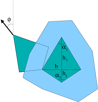
Figure 2: Sketches of the particle geometry and the excluded area of two kites for a relative angle $\phi$. Some characteristic lengths and angles are shown.

Considering that $\alpha_{1}\leq\alpha_{2}$ (as sketched in Fig. 2), the SPT area, $A_{\rm spt}(\phi)=A_{\rm excl}(\phi)-2a$, with a relative angle $0\leq\phi\leq\pi$ can be calculated from

$$A_{\rm spt}(\phi) = 2l_{1}^{2}\sin\alpha_{1}\cos\phi$$ (17)

$$+ l_{1}^{2}\sin(\phi-\alpha_{1})\Theta(\phi-\alpha_{1})$$

$$+ l_{2}^{2}\sin(\phi-\alpha_{2})\Theta(\phi-\alpha_{2})$$

$$+ 2l_{1}l_{2}\left[\sin(\phi-\alpha_{12}^{-})\Theta(\phi-\alpha_{12}^{-})\right.$$

$$+ \left.\sin(\phi-\pi+\alpha_{12}^{+})\Theta(\phi-\pi+\alpha_{12}^{+})\right].$$

Here we have defined $\alpha_{12}^{\pm}=(\alpha_{2}\pm\alpha_{1})/2$, and $\Theta(x)$ is the Heaviside function. For $\pi\leq\phi\leq 2\pi$ the SPT area is just $A_{\rm spt}(2\pi-\phi)$.

In general, kites are not symmetric with respect to $180^{\circ}$ rotations. However, as we showed in Ref. MR2 , a fluid of hard triangles (also a non-symmetric particle) has equilibrium N and TR phases with orientational distribution functions having the symmetry $h(\phi)=h(\pi-\phi)$, a property directly related to the nonnegativity of the odd-index Fourier amplitudes of the function $A_{\rm spt}(\phi)$ MR2 :

$$\int_{0}^{2\pi}d\phi\cos[(2k-1)\phi]A_{\rm spt}(\phi)=\left\{\begin{matrix}0,&k=1,\\ >0,&k>1.\end{matrix}\right.$$ (18)

The function $A_{\rm spt}(\phi)$ for kites also exhibits the same property. This symmetry of the orientational distribution function implies that particles axes have equal probabilities to point along the two possible directions parallel to the (N,T,TR)-directors.

By construction kites can degenerate into squares if $\alpha_{1}=\alpha_{2}=90^{\circ}$, into triangles when $\alpha_{2}=180^{\circ}$ and $\alpha_{1}<180^{\circ}$, or into rhombuses for $\alpha_{1}=\alpha_{2}$. Fig. 3 shows four examples of the function $A_{\rm spt}(\phi)$ for squares, equilateral triangles ($\alpha_{1}=60^{\circ}$ $\alpha_{2}=180^{\circ}$), rhombuses with $\alpha_{1}=\alpha_{2}=60^{\circ}$ and also for kites with $\alpha_{1}=60^{\circ}$ and $\alpha_{2}=240^{\circ}$. The symmetries of this function are: (i) $A_{\rm spt}(\phi)=A_{\rm{spt}}(\phi+\pi/2)$ for squares, (ii) $A_{\rm spt}(\phi)=A_{\rm{spt}}(\phi+2\pi/3)$ for equilateral triangles, and (iii) $A_{\rm spt}(\phi)=A_{\rm{spt}}(\pi-\phi)$ for rhombuses. These symmetries are directly related to the propensity of the system to stabilize the T, TR and N phases, respectively, at high densities. Also note the complexity of $A_{\rm spt}(\phi)$ for kites with $\alpha_{1}=60^{\circ}$ and $\alpha_{2}=120^{\circ}$ (this is generally true for $\alpha_{1}\neq\alpha_{2}$), with the presence of several local minima and maxima, and with the absolute minimum always located at $\phi=\pi$. Thus the minimum excluded area is always reached when the main particle axes are antiparallel, resulting in $A_{\rm excl}(\pi)=4a$.

Figure 3: The function $A_{\rm spt}(\phi)$ for squares (dashed), triangles with $\alpha_{1}=60^{\circ}$ and $\alpha_{2}=180^{\circ}$ (dotted), rhombuses with $\alpha_{1}=\alpha_{2}=60^{\circ}$ (dot-dashed) and kites with $\alpha_{1}=60^{\circ}$ and $\alpha_{2}=120^{\circ}$ (solid).

II.3 Bifurcation analysis from I phase

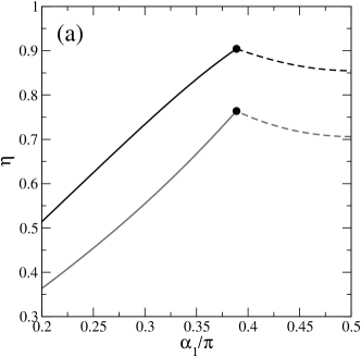
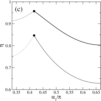
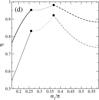
Figure 4: I-N (solid), I-T (dashed) and I-TR (dotted) bifurcation curves of (a) hard rhombuses, (b) kites with $\alpha_{1}+\alpha_{2}=180^{\circ}$, (c) $240^{\circ}=4\pi/3$ and (d) $210^{\circ}=7\pi/6$, according to SPT (black) and the new approach (dark grey). Intersections between these curves are shown by black circles. Intervals of the opening angle $\alpha_{1}$ shown in (c) and (d) are $[\pi/3,2\pi/3]$ and $[\pi/6,7\pi/12]$, respectively.

In this section we present the calculation of the second order transition lines, $\eta$ as a function of the opening angle $\alpha_{1}$ of kites, from the I to orientationally ordered phases, using some constraints on the other angle $\alpha_{2}$. As shown in Sec. III these transitions can be of first order. However this generally occurs in a small region of the phase diagram, so the I-(TR,T,N) transitions are, for most values of $\alpha_{1}$, of second order.

Inserting the Fourier expansion (16) into the definition of $\gamma[h]$, Eq. (6), we obtain

$$\gamma[h]=\gamma_{0}+\frac{1}{2}\sum_{k\geq 1}\gamma_{k}h_{k}^{2},$$ (19)

where we define the coefficients

$$\gamma_{k}\equiv\frac{1}{\pi}\int_{0}^{\pi}d\phi\frac{A_{\rm spt}(\phi)}{2a}\cos(2k\phi)$$

$$=-\frac{\left[\sin(\alpha_{1}/2)\cos(k\alpha_{2})+\sin(\alpha_{2}/2)\cos(k\alpha_{1})\right]^{2}}{\left(4k^{2}-1\right)\pi\sin(\alpha_{1}/2)\sin(\alpha_{2}/2)\sin\left[(\alpha_{1}+\alpha_{2})/2\right]},$$ (20)

depending only on $\alpha_{i}$ ($i=1,2$). Note that we used the symmetry of $A_{\rm spt}(\phi)$ with respect to the axis $\phi=\pi$ to integrate from 0 to $\pi$, multiplying the result by 2. In the following we use the same symmetry of $h(\phi)$ to change the integration intervals from $[0,2\pi]$ to $[0,\pi]$. Because of this, the normalization factor $(2\pi)^{-1}$ in $h(\phi)$ (see Eq. (16)) will be substituted by $\pi^{-1}$.

Consider a small perturbation of the orientational distribution function of the I phase, $h(\phi)\approx\pi^{-1}\left(1+h_{j}^{2}\cos(2j\phi)\right)$, where $j=1,2$ and 3 for N, T, and TR symmetries, respectively. The lowest order perturbation of the ideal part of the free-energy per particle is $\displaystyle{\varphi_{\rm id}\approx\log\eta-1+\frac{h_{j}^{2}}{4}}$, while the excess part can be calculated from (13), taking

$$\gamma[h]\approx\gamma_{0}+\frac{1}{2}\gamma_{j}h_{j}^{2},$$ (21)

and retaining only terms proportional to $h_{j}^{2n}$ (with $n=0,1$). The free-energy difference between the orientationally ordered phase $\rm{X}$ ($\rm{X}=$N, T, TR) and the I phase is

$$\Delta\varphi\equiv\varphi_{\rm X}-\varphi_{\rm I}\simeq\left\{1+2\left[\frac{\eta}{1-\eta}+(2\gamma_{0}-1)\left(\frac{1}{2}+r\eta\right)\right.\right.$$

$$\left.\left.\hskip 28.45274pt\times\left(\frac{\eta}{1-\eta}+\log(1-\eta)\right)\right]\gamma_{j}\right\}\frac{h_{j}^{2}}{4}.$$ (22)

At the bifurcation point the factor inside the square bracket is equal to zero. The value of the packing fraction at this point is obtained by solving (22) numerically for $\eta$. Considering now the free-energy difference from the SPT approach, i.e. the same Eqn. (22) but removing the term proportional to $2\gamma_{0}-1$, we obtain a simple analytical result:

$$\eta_{j}=\frac{1}{1-2\gamma_{j}},$$ (23)

where the packing fraction is labeled with $j$, indicating the symmetry of the bifurcated phase. Some interesting cases are: rhombuses with $\alpha_{1}=\alpha_{2}$, and kites with $\alpha_{1}+\alpha_{2}=180^{\circ}$. The latter constraint implies that the other two equal angles of the kites are fixed to $90^{\circ}$. As shown below this restriction constitutes an important requirement for a stable T phase even for values of $\alpha_{1}$ significantly different from $90^{\circ}$ (square geometry). The expressions for $\eta_{j}$ for these important cases are

$$\frac{1}{\eta_{j}}=\left\{\begin{array}[]{l}1+\frac{8\cos^{2}(j\alpha_{1})}{\pi(4j^{2}-1)\sin\alpha_{1}}\hskip 71.13188pt(\alpha_{1}=\alpha_{2})\\ \\ 1+\frac{2\cos^{2}(j\alpha_{1})\left[\tan(\alpha_{1}/2)+\cot(\alpha_{1}/2)+2(-1)^{j}\right]}{\pi(4j^{2}-1)}\\ \hskip 136.5733pt(\alpha_{1}+\alpha_{2}=\pi).\end{array}\right.$$ (28)

(29)

A first indication for the stability of the T phase in a fluid of hard rhombuses is given by the intersection of the I-N ($j=1$) and I-T ($j=2$) bifurcation curves, $\eta_{1}(\alpha_{1})=\eta_{2}(\alpha_{1})$. This equality gives the result $\alpha_{1}^{*}\simeq 69.98^{\circ}$, a value corresponding to the most anisometric rhombus with a stable T phase. In fact the actual value is a bit larger since, as shown in Sec. III, the phase transitions are of first order in the neighborhood of the intersection point. For the case $\alpha_{1}+\alpha_{2}=180^{\circ}$ the solution to the equation $\eta_{1}(\alpha_{1})=\eta_{2}(\alpha_{1})$ is $\alpha_{1}^{*}=56.14^{\circ}$. Obviously the fact that the other two equal angles of the kites are $90^{\circ}$ promotes the stabilization of the T phase for values of $\alpha_{1}$ lower to those for hard rhombuses.

Applying now the constraint $\alpha_{1}+\alpha_{2}=240^{\circ}$, we obtain the I-N and I-TR bifurcation curves

$$\frac{1}{\eta_{j}}=\left\{\begin{matrix}1+\frac{\cos^{2}(3\alpha_{1}/2)}{\sqrt{3}\pi\sin(\alpha_{1}/2)\sin(\alpha_{1}/2+\pi/3)}&(j=1)\\ &\\ 1+\frac{4\sqrt{3}\cos^{2}(3\alpha_{1})\cos^{2}(\alpha_{1}/2-\pi/3)}{35\pi\sin(\alpha_{1}/2)\sin(\alpha_{1}/2+\pi/3)}&(j=3).\end{matrix}\right.$$ (30)

In this case the equal angles of the kites are fixed to $60^{\circ}$. Thus for $\alpha_{1}=60^{\circ}$ the kite degenerates into an equilateral triangle while for $\alpha_{1}=120^{\circ}$ it becomes a rhombus. The equality $\eta_{1}(\alpha_{1})=\eta_{3}(\alpha_{1})$ gives $\alpha_{1}^{*}\simeq 75^{\circ}$. This value is rather close to $60^{\circ}$, implying that the TR phase is less stable with respect to deformations (within the kite geometry) of the equilateral triangle as compared to rhombuses or kites with $\alpha_{1}+\alpha_{2}=180^{\circ}$. In fact the difference $\Delta\alpha_{1}\equiv\left|\alpha_{1}^{*}-\alpha_{1}^{\rm ref}\right|$ (with $\alpha_{1}^{\rm ref}=90^{\circ}$ for rhombuses and kites with $\alpha_{1}+\alpha_{2}=180^{\circ}$, and $\alpha_{1}^{\rm ref}=60^{\circ}$ for kites with $\alpha_{1}+\alpha_{2}=240^{\circ}$), gives $\Delta\alpha_{1}\approx 15^{\circ}$, $20^{\circ}$ and $34^{\circ}$ for $240^{\circ}$-kites, rhombuses and $180^{\circ}$-kites, respectively.

Fig. 4 shows the bifurcation curves for the I-N transition, $\eta_{1}(\alpha_{1})$, and the I-T transition, $\eta_{2}(\alpha_{2})$, for (a) rhombuses and (b) kites with $\alpha_{1}+\alpha_{2}=180^{\circ}$, as obtained from Eqns. (29). Panel (c) corresponds to $\eta_{1}(\alpha_{1})$ and $\eta_{3}(\alpha_{1})$ (the I-TR bifurcation) for the case $\alpha_{1}+\alpha_{2}=240^{\circ}$, obtained from Eqns. (30). All figures also show the same bifurcation curves from the new approach (with $r=2$). Finally in (d) the case $\alpha_{1}+\alpha_{2}=210^{\circ}$ is shown. It is clear that the new approach gives much lower values of packing fractions at bifurcation than those predicted from the SPT for all the explored values of $\alpha_{1}$. However the intersections between different bifurcation curves (which can be taken to approximately bound the stability regions of the N, T and TR phases), are located at the same values $\alpha_{1}^{*}$. This result can be explained by the fact that the equality $\eta_{i}(\alpha_{1})=\eta_{j}(\alpha_{1})$ implies the same equality $\gamma_{i}=\gamma_{j}$ for both theories.

The stability of the N, T and TR phases is bounded from below, in case of second order transitions, by the bifurcation curves plotted in Fig. 4. However, as shown in Sec. III, the T and TR phases exhibit a transition to a N phase at high densities. Also nonuniform phases, not taken into account in the present study, could limit the stability of the orientationally ordered phases from above. To calculate the (T,TR)-N second order transitions, we need to perform a bifurcation analysis from T and TR phases, which we relegate to Sec. A.

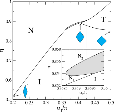
Figure 5: Phase diagram of hard rhombuses ($\alpha_{1}=\alpha_{2}$) in the packing fraction ($\eta$)-opening angle ($\alpha_{1}$) plane. The regions of stability of I, T and N phases are correspondingly labeled. The coexistence region of the I-N and T-N first-order phase transitions (located in the neighborhood of the crossover between the I-T and T-N bifurcation curves) are shaded in grey. The inset shows a detail of the N₁-N₂ first-order phase transition in a small $\alpha_{1}$ interval. Also rhombuses for different $\alpha_{1}$ are depicted, in particular the one located at the intersection of the I-T second-order transition curve with the (I,TR)-binodal of the I-N (left) and TR-N (right) transitions.

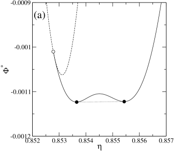
Figure 6: (a) Free-energy densities of I (dashed) and N (solid) phases vs. packing fraction of hard rhombuses with $\alpha_{1}=0.359\pi=64.62^{\circ}$. We have defined $\Phi^{*}=\Phi+53.344-71.474\eta$, where a straight line has been subtracted from the free-energy. N-N coexistence is shown by black circles joined by a dotted line. The open circle indicates the I-N bifurcation point. (b) The functions $h(\phi)$ corresponding to the N₁ (dashed)-N₂ (solid) coexistence (the black circles of panel (a)). (c) Orientational distribution function $h(\phi)$ of the N phase coexisting with I for rhombuses with $\alpha_{1}=0.4\pi=72^{\circ}$. (d) The functions $h(\phi)$ corresponding to the T (dashed) and N (solid) phases of rhombuses with $\alpha_{1}=0.42\pi=75.6^{\circ}$.

The case of kites with $\alpha_{1}+\alpha_{2}=210^{\circ}=7\pi/6$ deserves special attention. When $\alpha_{1}=30^{\circ}$ and consequently $\alpha_{2}=180^{\circ}$, the kite degenerates into an acute isosceles triangle, while for $\alpha_{1}=\alpha_{2}=105^{\circ}=7\pi/12$ particle becomes a rhombus. For larger values of $\alpha_{1}$ the phase diagram is symmetric with respect to the axis $\alpha_{1}=105^{\circ}$. From Fig. 4(d) we see that the N, T and TR phases are present in the phase diagram, but the most striking feature is the existence of a crossover between the I-TR and I-T bifurcation curves. This could imply that there exist some kites which can have stable T and TR phases and a transition between them. In Sec. III this case is studied in detail, and we will show that below this crossover the I phase exhibits a transition to the N phase, with the latter being the stable one at high densities.

III Results

This section is divided into three parts, each showing the phase diagrams as well as the orientational properties of: rhombuses (Sec. III.1), kites with the sum of the two unequal interior angles constant, $\alpha_{1}+\alpha_{2}=\text{const}$ (Sec. III.2), and kites with one of the unequal interior angles fixed to $\alpha_{1}=72^{\circ}$ (Sec. III.3).

III.1 Hard rhombuses

First we calculated the phase diagram of the uniform phases of hard rhombuses ($\alpha_{1}=\alpha_{2}$). Apart from the I-N and I-T bifurcation curves, shown in Fig. 4 (a), we also calculated the T-N bifurcation curve using the formalism described in Sec. A. Also for those values of $\alpha_{1}$ where a first order I-N or T-N transition exists, we calculated the coexisting packing fractions from the equality of chemical potential and pressure of the coexisting phases. The complete phase diagram is shown in Fig. 5. We can see how the region of stability of the T phase is reduced as the particle shape changes from square ($\alpha_{1}=90^{\circ})$ to a critical rhombus with $\alpha_{1}=73^{\circ}$ (shown in the figure). The stability region of the T phase is bounded below and above by the I-N and T-N second-order transition curves. In the neighborhood of their intersection there exists an interval of $\alpha_{1}$ where first-order I-N and T-N transitions take place. For $\alpha_{1}$ below the intersection of the I-N bifurcation curve and the I-binodal of the I-N transition, there exists a N-N transition ending in a critical point. The N-N coexistence region is shown in the inset of Fig. 5.

Obviously for small values of $\alpha_{1}$, when the rhombus becomes highly elongated, the N phase is the only possible uniform phase with orientational order at high enough densities. This phase becomes stable at a second-order I-N transition, occurring at rather low packing fraction. For $\alpha_{1}\sim 90^{\circ}$ the T phase is the stable one at densities above a second-order I-T transition, at relative high packing fractions. As the opening angle decreases from $90^{\circ}$ and reaches a critical value $\alpha_{1}^{*}=73^{\circ}$, the T phase looses its stability. For $\alpha\gtrsim\alpha_{1}^{*}$, as the density increases, the T phase exhibits a transition to a N phase (see Fig. 5), so that particle axes break the fourfold symmetry and the alignment along two equivalent directors changes to alignment along a single director. However, as the structure of the function $h(\phi)$ indicates, this N phase keeps some tetratic correlations. As shown below, in the interval $[0,360^{\circ}]$ the function still exhibits four peaks separated by $90^{\circ}$, but two of them, separated by $180^{\circ}$, are much sharper and consequently the T symmetry is broken. The present results indicate that the second-virial DFT theories predict, for opening angles close to the critical value $\alpha_{1}^{\ast}$, the existence of first order I-N, T-N and N-N transitions, all of them coalescing in the same region of the phase diagram.

The free-energy density $\Phi\equiv\beta{\cal F}a/A=\eta\varphi$ as a function of $\eta$ for $\alpha_{1}=0.359\pi=64.62^{\circ}$ is shown in Fig. 6(a). The free energy clearly shows the presence of a N-N transition. In panel (b) the coexisting orientational distribution functions for both uniaxial nematics for this value $\alpha_{1}$ are shown. Panel (c) shows the function $h(\phi)$ of the N phase that coexists with the I phase, for a value $\alpha_{1}=0.4\pi=72^{\circ}$ (located within the I-N first order transition region). We see the strong uniaxial ordering, with the presence of sharp peaks located at $\phi=0,180^{\circ}$, and the existence of small undulations around $\phi=90^{\circ}$. Finally, in panel (d) we show $h(\phi)$ for the coexisting T and N phases at $\alpha_{1}=0.42\pi=75.6^{\circ}$. The former has three peaks with equal heights, located at $\phi=\left\{0,90^{\circ},180^{\circ}\right\}$, indicating the T symmetry $h(\phi)=h(\phi+\pi/2)$, while the latter exhibits a clear uniaxial character with the most pronounced peaks located at $\phi=\left\{0,180^{\circ}\right\}$, and with a secondary peak located at $\phi=90^{\circ}$, corresponding to the presence of T correlations.

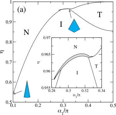
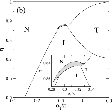
Figure 7: Phase diagrams of kites with $\alpha_{1}+\alpha_{2}=180^{\circ}$ according to (a) SPT, and (b) the new approach. The insets show the regions of the phase diagrams where first-order transitions take place. Coexistence regions are shaded in grey. The stability regions of I, N and T phases are correspondingly labeled. In (a) kites for two values of $\alpha_{1}$ are depicted.

III.2 Hard kites with $\alpha_{1}+\alpha_{2}=\text{const}$

The next phase diagram is that of kites with the constraint $\alpha_{1}+\alpha_{2}=180^{\circ}$, i.e. with the two equal angles fixed to $90^{\circ}$. We have used both, the SPT, and the new approach discussed in Sec. II.1. Results are plotted in Fig. 7(a) and (b), respectively. The fact that two of the angles of kites are right angles makes the averaged excluded area to decrease much more, as T ordering increases from the orientationally disordered configuration. If MC simulations of kites with $\alpha_{1}+\alpha_{2}=180^{\circ}$ were performed they presumably would show a high propensity of particles to form clusters of particles joined by the sides adjacent to the right-angled vertexes. In turn the presence of a large amount of these clusters with $\alpha_{1}$ not acute enough is the main stabilizing mechanism for the T phase. This result is confirmed in Fig. 7 where, according to both theories, the lower limit of stability of the T phase is reached for $\alpha_{1}\approx 58.4^{\circ}$, a critical angle significantly lower than that for rhombuses. In the region where the I-N, I-T and T-N bifurcation curves meet we again observe the existence of first-order phase transitions between different phases, with the presence of a N-N transition ending in a critical point. Interestingly the $\alpha_{1}$-interval where the latter occurs is enlarged with respect to that of rhombuses and also takes place at higher densities. By comparing both panels we conclude that, within the new approach, the region of stability of the T phase is significantly enlarged, with the second-order I-T transition occurring at lower densities. Also the I-N, T-N and N-N first-order transitions become stronger, with a wide density gap.

Figure 8: Orientational distribution functions, $h(\phi)$ for two coexisting nematics, N₁ (dashed) and N₂ (solid) of kites with $\alpha_{1}=0.285\pi=51.3^{\circ}$ and $\alpha_{1}+\alpha_{2}=180^{\circ}$ calculated from SPT. Inset: the SPT-area, $A_{\rm spt}(\phi)$, for these kites.

In Fig. 8 the orientational distribution functions of two coexisting nematics of kites with $\alpha_{1}=0.285\pi=51.3^{\circ}$, as calculated from SPT, are plotted. The function $h(\phi)$ for the higher-ordered nematic ($N_{2}$) has, apart from the main peaks located at $\left\{0,180^{\circ}\right\}$, three additional local maxima, whose locations are strongly correlated with the particle shapes. This can be seen in the inset, where we plot the function $A_{\rm spt}(\phi)$ for this value of $\alpha_{1}$. Two of the local minima of $A_{\rm spt}(\phi)$ are located at $\alpha_{1}=0.285\pi=51.3^{\circ}$ and $90^{\circ}$ (highly correlated with two of the positions of the local maxima of $h(\phi)$), with the other being the symmetric counterpart of that located at $\phi\approx 0.233\pi=41.94^{\circ}$. The latter is inside the interval $[0.215\pi,0.285\pi]$, where the function $A_{\rm spt}(\phi)$ has a relatively low value. Thus, apart from the most favored antiparallel orientations of the main particle axes ($\left\{0,180^{\circ}\right\}$), some orientations are also favored to a lesser extent, due to the local minimization of the excluded area.

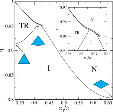
Figure 9: Phase diagram of kites with $\alpha_{1}+\alpha_{2}=240^{\circ}$. The inset shows a detail close to the intersection between the I-N and I-TR bifurcation curves. The regions shaded in grey indicate the first order character of phase transitions. Regions of stability of I, TR and N phases are correspondingly labeled. Three kites with $\alpha_{1}=60^{\circ}$, $\alpha_{1}=74.3^{\circ}$ and $\alpha_{1}=120^{\circ}$ are depicted, the middle indicating the upper stability limit of TR phase.

We have calculated the phase diagram of kites with the constraint $\alpha_{1}+\alpha_{2}=240^{\circ}$ and $\alpha_{1}\in[60^{\circ},120^{\circ}]$ with the aim to study in what extent the TR phase, with the symmetry $h(\phi)=h(\phi+\pi/3)$, is still stable by deforming an equilateral triangle within the kite geometry. The results from the SPT are plotted in Fig. 9 which shows that the region of TR phase stability, bounded by I-TR bifurcation curve and the TR-coexistence binodal of TR-N transition, ends at $\alpha_{1}\approx 74.3^{\circ}$ (see the shape of this kite in Fig. 9) a value not too far from $60^{\circ}$ indicating that the TR phase is very sensitive to these kind of deformations. Also, in the region where the I-TR and I-N bifurcation curves meet, the I-N transition becomes of first order (see the inset) which continues in a TR-N transition for lower $\alpha_{1}$ eventually keeping its first order character up to $\alpha_{1}=60^{\circ}$. We can only speculate about this fact close to $\eta\approx 1$ because the coexistence calculations are very difficult to numerically perform in this limit so we extrapolated the obtained TR and N binodals up to $\eta=1$.

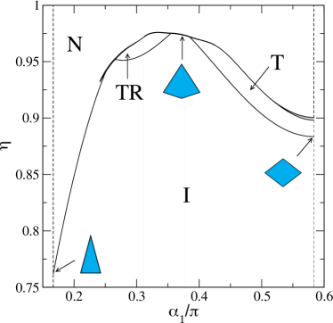
Figure 10: Phase diagram of kites with $\alpha_{1}+\alpha_{2}=210^{\circ}$ following the SPT. Regions of stability of I, TR and N phases are correspondingly labeled. Some kites are sketched.

As we have already pointed out in Sec. II.3 kites with $\alpha_{1}+\alpha_{2}=210^{\circ}$ and $\alpha_{1}\in[30^{\circ},105^{\circ}]$ deserve special attention for two reasons: (i) from the bifurcation analysis we showed that the T and TR phases are present in the phase diagram and (ii) it is interesting to prove or discard the existence of a kite with both T and TR phases and a transition between them. The complete phase diagram resulting from the SPT is plotted in Fig. 10. Indeed the TR and T phases are stable and they are bounded above by a TR or T binodals of the (TR,T)-N first order phase transitions except for some relatively small intervals of $\alpha_{1}$ where these transitions becomes of second order. Two examples of equilibrium orientational distribution functions $h(\phi)$ for stable T and TR phases, with their inherent symmetries $h(\phi+2\pi/n)$ (with $n=4$ and 6 for T and TR respectively), are shown in Fig. 11 (a). As we can see from the phase diagram of Fig. 10, for values of $\alpha_{1}$ close to that of the intersection between I-TR and I-T bifurcation curves [see also Fig. 4 (d)] the I phase exhibits a direct transition to a N phase thus discarding at all the existence of a particle geometry having both stable TR and T phases. Also the packing fraction values at which the TR and T phases are stable are remarkable high if we compare with those of the other phase diagrams shown. Thus we expect that if we included the nonuniform phases in our analysis they would be more stable than the orientationally ordered uniform phases in large parts of the phase diagram.

Figure 11: (a) Orientational distribution functions of kites with $\alpha_{1}+\alpha_{2}=210^{\circ}$ and values of the pairs $(\alpha_{1},\eta)=\left(54^{\circ},0.965\right)$ (solid) and $\left(90^{\circ},0.922\right)$ (dashed), corresponding to stable TR and T phases, respectively. (b) Three different functions $h(\phi)$ corresponding to stable N phases of kites with $(\alpha_{1},\eta)=\left(54^{\circ},0.971\right)$ (dotted), $\left(66.6^{\circ},0.975\right)$ (solid) and $\left(90^{\circ},0.935\right)$. The scale of the figure has been chosen so as to enhance the secondary peaks of $h(\phi)$.

In Fig. 11 (b) we plot the function $h(\phi)$ for three different stable N phases for values of the opening angle of kites $\alpha_{1}=0.3\pi=54^{\circ}$, $0.37\pi=66.6^{\circ}$ and $90^{\circ}$ and for packing fractions higher than upper bounds of stability of TR, I and T phases respectively (see the phase diagram of Fig. 10). We concentrate only on the description of the secondary peaks (the much sharper main peaks are located at $\{0,\pi\}$ and are outside the scale of the figure). For packing fractions above the TR-phase stability region (fixing $\alpha_{1}=0.3\pi$) the secondary peaks of the stable N phase are located at $\phi\approx\{\pi/3,2\pi/3\}$ confirming the presence of important TR correlations in particle orientations. As $\alpha_{1}$ increases up to $0.37\pi$, approximately coinciding with the location of the intersection between the I-TR and I-T bifurcation curves, these main secondary peaks move to $\phi\approx 0.4\pi$ and $0.6\pi$, approximately equal to $\alpha_{1}$ and its symmetric counterpart with respect to $0.5\pi$. As we have already described above this issue is related with the local minima of the function $A_{\rm spt}(\phi)$. It is interesting also to observe the presence of two lower peaks located at $\phi\approx 0.2\pi$ and $0.8\pi$ which are also related with the structure of the excluded area. Finally for $\alpha_{1}=0.5\pi$ (the right opening angle) we observe the usual secondary peak located of $\phi=\pi/2$ showing the presence of important T correlations in the fluid.

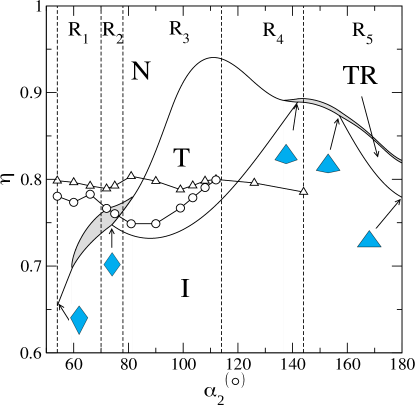
Figure 12: Phase diagram of hard kites with one of the unequal interior angles set to $\alpha_{1}=72^{\circ}$, while the other one is varied in the interval $[54^{\circ},180^{\circ}]$. Results correspond to the new approach for $\varphi_{\rm exc}[h]$, with $r=2$. The regions of stability of I, N, T and TR phases are correspondingly labeled. Shaded regions indicate the coexistence regions of the first-order phase transitions. Open circles and triangles show transitions from I to liquid-crystalline uniform phases and from uniform to non-uniform phases, respectively, as obtained from the MC simulations of Ref. zhao1 . Different regions, from R₁ to R₄, correspond to the division of the interval $[54^{\circ},144^{\circ}]$ introduced by the authors of Ref. zhao1 ; from left to right, these regions indicate the stability intervals for H^mo phase (see the text for its definition), an asymmetric tetratic phase T₂, and the usual symmetric T₁ phase. In region R₅ (not calculated in Ref. zhao1 ), the presence of a TR phase is observed.

III.3 Hard kites with $\alpha_{1}=72^{\circ}$

Finally, we have calculated the phase diagram of kites with one of the unequal opening angles fixed to $\alpha_{1}=72^{\circ}$, while the other one, $\alpha_{2}$, was varied inside the interval $[54^{\circ},180^{\circ}]$. The new approach for $\varphi_{\rm exc}[h]$ with $r=2$ [see Eq. (13)] was used. The aim of this calculation was to compare the results obtained from the implementation of our new theoretical model with recent MC simulations of hard kites with the same value of $\alpha_{1}$ and with $\alpha_{2}\in[54^{\circ},144^{\circ}]$ zhao1 . In Fig. 12 the theoretical phase diagram, together with the simulation results of Ref. zhao1 , are shown. Our model predicts that, as $\alpha_{2}$ is varied from $54^{\circ}$ to $180^{\circ}$, the I phase exhibits a sequence of transitions to N ($\alpha_{2}\in[54^{\circ},74^{\circ}]$), T ($\alpha_{2}\in[74^{\circ},142^{\circ}]$), N again ($\alpha_{2}\in[142^{\circ},157^{\circ}]$), and TR ($\alpha_{2}\in[157^{\circ},180^{\circ}]$) phases. The I-N transitions are generally of first order.

Considering only uniform phases, our analysis shows that the T and TR phases are stable up to packing fractions where second- or first-order (T,TR)-N transitions occur. Fig. 12 shows the transitions from the I to liquid-crystalline phases (open circles) and from these to non-uniform phases (open triangles), as obtained from the MC simulations of Ref. zhao1 . The authors of Ref. zhao1 divided the interval $[54^{\circ},144^{\circ}]$ in four regions (enumerated in Fig. 12 using the labels R_i, with $i=1,\dots,4$). They claimed the existence of: (i) a molecular ordered hexatic liquid-crystal phase (H^mo) (in principle, this is what we call here a TR phase) in R₁, (ii) an asymmetric T phase (T₂) in R₂, (iii) the usual symmetric T phase (T₁) in R₃, and (iv) a direct transition from I to non-uniform phases in R₄.

From the structure of $h(\phi)$ in the region R₁, with six peaks separated by $60^{\circ}$ but not necessarily of the same height, the authors of Ref. zhao1 concluded that H^mo is stable in a relatively small interval of $\eta$. In R₂ they found an angular distribution $h(\phi)$ with four peaks separated by $90^{\circ}$, but these come in pairs of different height, so this was associated to an asymmetric T (T₂) phase. Finally, in R₃ a distribution with nearly perfect fourfold symmetry was found, which points to the usual T phase, called T₁.

From the theoretical point of view, however, the definitions of the T and TR phases are clearcut: the symmetry $h(\phi)=h(\phi+2\pi/n)$ (with $n=4$ and $6$, respectively) must be fulfilled. In case $h(\phi)\neq h(\phi+2\pi/n)$ the phase should be called N, even if the secondary peaks of $h(\phi)$ (different from the main ones at $\{0,\pi\}$) are sharp, pointing to important T or TR correlations in the fluid.

Fig. 13(a) shows the function $h(\phi)$ for the coexisting N phase at the I-N transition, for kites with $\alpha_{2}=70^{\circ}$ (just at the boundary between R₁ and R₂). For values of $\alpha_{2}$ well inside the region $R_{1}$, the structure of $h(\phi)$ is similar, except for the precise location of the secondary peaks, which change with $\alpha_{2}$. In this case, from the structure of $h(\phi)$ we can infer the existence of clear N ordering, with two sharp peaks at $\{0,\pi\}$, and two very small secondary peaks at $\phi\approx\{0.4\pi,0.6\pi\}$, separated by a region with a rather constant value and a weak local minimum at $\phi=0.5\pi$. This approximate plateau in the interval $0.4\pi$ to $0.6\pi$ indicates the existence of T correlations which, as can be seen from panel (b), are much stronger in the N phase coexisting with T for kites with $\alpha_{2}=78^{\circ}$ (a value close to the boundary between the regions R₂ and R₃). For $\alpha_{2}\in[54^{\circ},70^{\circ}]$ we only see a uniaxial N phase with very small TR correlations.

Figure 13: (a) Coexisting N distributions corresponding to the I-N transitions of hard kites with $\alpha_{1}=72^{\circ}$, and $\alpha_{2}=70^{\circ}$ (dashed) and $150^{\circ}$ (solid). (b) Coexisting distributions corresponding to the T (dashed)-N (solid) transition for kites with same the $\alpha_{1}$ and $\alpha_{2}=78^{\circ}$. (c) Coexisting distributions of the TR (dashed)-N (solid) transition for kites with the same $\alpha_{1}$ and $\alpha_{2}=171^{\circ}$.

The structure of the asymmetric distribution found in R₁ by the simulations is more similar to that we found in the N phase (coexisting with I) of kites with $\alpha_{2}=150^{\circ}$, see panel (a), or in the N phase (coexisting with TR) of kites with $\alpha_{2}=171^{\circ}$, see the panel (c); both these values are inside the region R₅.

Differences in the heights of the secondary peaks of $h(\phi)$ resulting from theory and simulations, with $\alpha_{2}$ well inside the region R₁, could be explained by the importance of three-body and higher correlations in the description of the ordering properties of the fluid. Our theory approximates the third virial coefficient of the N phase based on the second, which could explain the differences mentioned above.

Despite this, following our definitions for the orientationally ordered phases and renaming H^mo to N and T₂ to N, the phase diagrams of MC simulations and theory are remarkable similar, in particular regarding the stability of uniform orientationally-ordered phases. The I-N transition occurs in the regions R₁ and R₂, the I-T transition in R₃, and the transition from I to non-uniform phases in $R_{4}$, similar to what we found from the theoretical model (except for the presence of non-uniform phases). Also the packing fractions of these transitions are quite similar. The main drawback of the model is the impossibility to study the stability of non-uniform phases, which would require a DFT for the one-body density profile $\rho({\bm{r}},\phi)$ with an accurate description of spatial correlations. An extension of the present model involving the substitution $\rho(\phi)\to\rho({\bm{r}},\phi)$ is simply not adequate. The recently developed DFT based on the Fundamental Measure Theory fmt is expected to be a promising route.

The inclusion of non-uniform phases would probably modify the phase diagram of Fig. 12 in the sense that the region where the T is now stable for $\eta\gtrsim 0.8$ would become unstable with respect to spatially ordered phases. Taking this into account we obtain a confidence interval for T-phase stability as $\alpha_{2}\sim[74^{\circ},121^{\circ}]$, similar to that obtained from simulations where the region of T₁-stability is $\alpha_{2}\sim[78^{\circ},114^{\circ}]$.

Finally we would like to comment on the region in the phase diagram denoted by R₅. In this region, not simulated in Ref. zhao1 , we found that the I phase exhibits a transition to a TR phase for $\alpha_{2}\in[157^{\circ},180^{\circ}]$, as expected for kites similar to triangles and not very far from the equilateral triangle. This TR phase is stable up to packing fractions where a first-order TR-N transition takes place.

IV Conclusions

In this paper we have presented a systematic theoretical study of the phase behavior of hard kites, with an emphasis on the relative stability of all the possible uniform phases (I, T, TR and N). We used the SPT approximation, together with a new approach that approximates the third virial coefficient more accurately. This approximation was refined by comparing the EOS of hard squares from theory and MC simulations. Several phases diagrams were calculated, including that of rhombuses ($\alpha_{1}=\alpha_{2}$), a set of them for kites with a constraint on the sum of their two unequal interior angles, $\alpha_{1}+\alpha_{2}=\left\{180^{\circ},240^{\circ},210^{\circ}\right\}$, and finally that for kites with $\alpha_{1}=72^{\circ}$. The latter was calculated with the aim of comparing with recent MC simulations zhao1 . In general we found first- and second-order I-(T,TR,N) and (T,TR)-N transitions, which define regions of stability of the uniform phases. Also we found several intervals for the opening angle where the hard-kite fluid exhibits a first-order N-N transition ending in a critical point.

As expected, the T phase was found to be more stable for kites with both equal angles fixed to $90^{\circ}$ (the constraint $\alpha_{1}+\alpha_{2}=180^{\circ}$). For this particular case the interval of $\alpha_{1}$ where the T is stable is the largest, $[58.4^{\circ},90^{\circ}]$; compared to that of rhombuses: $[73^{\circ},90^{\circ}]$. The new approach presents a stabilizing effect on the T phase, with a dramatic lowering of the I-T bifurcation curve, resulting in a larger T-region in the phase diagram. Kites with the constraint $\alpha_{1}+\alpha_{2}=240^{\circ}$ and with an opening angle $\alpha_{1}$ within the interval $\left[60^{\circ},210^{\circ}\right]$ (with bounds corresponding to the equilateral triangle and rhombus respectively) have a stable TR phase for $\alpha_{1}\in[60^{\circ},74^{\circ}]$. We can therefore conclude that the TR phase is more sensitive to changes in particle shape (but still within the kite geometry) than the T phase. The case $\alpha_{1}+\alpha_{2}=210^{\circ}$ is particularly interesting because the crossover between the I-T and I-TR bifurcation curves would suggest the existence of some kites exhibiting transitions between T and TR phases. However, we have proved this is not possible due to the presence of an I-N transition occurring below the crossover, the N phase being the stable one at higher densities. The N phase close to the crossover is peculiar, in the sense that it presents TR or T correlations (depending on the value of $\alpha_{1}$), with the orientational distribution function $h(\phi)$ having secondary peaks (apart from the main peaks at $\left\{0,180^{\circ}\right\}$), located at angles $\phi$ compatible with those associated with the TR or T symmetries.

By comparing the phase diagrams of kites with $\alpha_{1}=72^{\circ}$ obtained from theory and simulations, we can validate the suitability of the new approach for the prediction of the stability of orientationally-ordered uniform phases. The interval of $\alpha_{1}$ where the T phase is stable and the densities of the I-T transition are quite similar in the theory and the simulations. Also similar is the structure of the orientational distribution function in some parts of the phase diagrams. In others this structure can be different, in particular regarding the relative heights of the secondary peaks, something that can be explained by the approximations, inherent in the theory, for the third and higher-order virial coefficients.

The inclusion of non-uniform phases deserves further study. This is certainly far from trivial at the DFT level. In this regard a DFT with an accurate description of spatial correlations would be required. An example of such a theory, developed for hard discorectangles and within the Fundamental Measure Formalism, can be found in Ref. fmt .

Appendix A Bifurcation analysis from (T,TR) phases

The starting point in the bifurcation analysis from the T or TR phases is the nonlinear integral equation resulting from the equilibrium condition:

$$\frac{\delta\varphi[h]}{\delta h(\phi)}=\lambda\Rightarrow h(\phi)=\exp{\left[\lambda-\frac{\delta\varphi_{\rm exc}[h]}{\delta h(\phi)}\right]},$$ (31)

where $\lambda$ is a Lagrange multiplier that guarantees the normalization $\int_{0}^{\pi}d\phi h(\phi)=1$. Taking into account Eqn. (13), we have

$$\frac{\delta\varphi_{\rm exc}[h]}{\delta h(\phi)}=\psi\left[h;\eta\right]\frac{\delta\gamma[h]}{\delta h(\phi)},$$

$$\frac{\delta\gamma[h]}{\delta h(\phi)}=\int_{0}^{\pi}d\phi^{\prime}h(\phi+\phi^{\prime})\frac{A_{\rm spt}(\phi^{\prime})}{a}$$

$$\hskip 85.35826pt=2\sum_{k\geq 0}\gamma_{k}h_{k}\cos(2k\phi),$$ (32)

where we have used the Fourier representation (16) of $h(\phi)$ and the definition (20) for the coefficients $\gamma_{k}$. Also the shorthand notation

$$\psi\left[h;\eta\right]=\frac{\eta}{1-\eta}+\left(2\gamma[h]-1\right)$$

$$\times\left(\frac{1}{2}+r\eta\right)\left(\frac{\eta}{1-\eta}+\log(1-\eta)\right).$$ (33)

has been used. From Eqs. (31) and (32) we obtain

$$h(\phi)=e^{\lambda}\exp{\left\{-2\psi\left[h;\eta\right]\sum_{k\geq 1}\gamma_{k}h_{k}\cos(2k\phi)\right\}},$$ (34)

where $\lambda$ can be calculated from

$$e^{-\lambda}=\int_{0}^{\pi}d\phi^{\prime}\exp{\left\{-2\psi\left[h;\eta\right]\sum_{k\geq 1}\gamma_{k}h_{k}\cos(2k\phi^{\prime})\right\}},$$ (35)

which obviously guarantees the normalization condition. Multiplying (34) by $\cos(2j\phi)$, integrating over $\phi$, and using again the expansion (16), we obtain

$$h_{j}=2e^{\lambda}\int_{0}^{\pi}d\phi\cos(2j\phi)$$

$$\times\exp{\left\{-2\psi\left[h;\eta\right]\sum_{k\geq 1}\gamma_{k}h_{k}\cos(2k\phi)\right\}}.$$ (36)

Now a small perturbation of the T phase is introduced, resulting in a N phase with orientation distribution function

$$h_{\rm N}(\phi)=h_{\rm T}(\phi)+\frac{1}{\pi}\sum_{j\geq 1}h_{2j-1}\cos[2(2j-1)\phi],$$

$$h_{\rm T}(\phi)=\frac{1}{\pi}\left(1+\sum_{j\geq 1}h_{2j}\cos(4j\phi)\right),$$ (37)

with $h_{2j-1}\ll h_{2j}$. We define the quantity

$$T(\phi)\equiv\exp{\left\{-\psi_{\rm T}\left[h;\eta\right]\sum_{k\geq 1}\gamma_{2k}h_{2k}\cos(4k\phi)\right\}},$$ (38)

with $\psi_{\rm T}\left[h;\eta\right]$ calculated from Eq. (33) with the anisometry parameter having a T symmetry:

$$\gamma_{\rm T}[h]=\gamma_{0}+\frac{1}{2}\sum_{k\geq 1}\gamma_{2k}h_{2k}^{2}.$$ (39)

Expanding Eqn. (36) for $j=2n-1$ up to first order in $\{h_{2k-1}\}$, and using the symmetry of the T phase (implying $\int_{0}^{\pi}d\phi T(\phi)\cos\left[2(2j-1)\phi\right]=0$), we obtain

$$h_{2n-1}=-\frac{2\psi_{0}(\eta)}{\int_{0}^{\pi}d\phi^{\prime}T(\phi^{\prime})}\int_{0}^{\pi}d\phi T(\phi)\sum_{k\geq 1}\gamma_{2k-1}h_{2k-1}$$

$$\times\left\{\cos[4(k+n-1)\phi]+\cos[4(k-n)\phi]\right\}$$ (40)

$$\Rightarrow h_{2n-1}=-\psi_{0}(\eta)\sum_{k\geq 1}\gamma_{2k-1}$$

$$\times\left[h_{2(k+n-1)}+h_{2|k-n|}\right]h_{2k-1}.$$ (41)

Here we have used the definition $h_{2k}=2\int_{0}^{\pi}d\phi T(\phi)\cos(4k\phi)/\int_{0}^{\pi}d\phi^{\prime}T(\phi^{\prime})$ while the function $\psi_{0}(\eta)$ is the same as (33) with the substitution $\gamma[h]\to\gamma_{0}$.

Defining now the column vector ${\bm{c}}$ with coordinates $c_{k}=h_{2k-1}$, $k=1,\dots,m/2$ (with $m$ an even number) and the matrix $B$ with elements

$$b_{nk}=\delta_{nk}+\psi_{0}(\eta)\gamma_{2k-1}\left(h_{2(k+n-1)}+h_{2|k-n|}\right),$$

$$\hskip 56.9055ptn,k=1,\dots,\frac{m}{2},$$ (42)

the Eqn. (41) can be put in the matrix form $B{\bm{c}}=\bm{0}$ which has a nontrivial solution for ${\bm{c}}$ if and only if

$${\cal B}(\eta,\{h_{2k}\})\equiv\text{det}\left(B\right)=0.$$ (43)

$m/2$ is the total number of even Fourier amplitudes $\{h_{1},h_{3},\dots,h_{m-1}\}$, which are of same order, say $\sim\epsilon$, in the perturbative expansion of $h(\phi)$ around $h_{\rm T}(\phi)$. We need to take $h_{2(k+n-1)}=0$ if $k+n-1>m/2$ and $h_{2|k-n|}=2$ for $k=n$.

We solve Eqn. (43) iteratively for the present as well as for the SPT approach (obtained by replacing $2\gamma_{0}-1$ by $0$ in Eqn. (33)) to find the T-N bifurcation value of $\eta$, once the equilibrium Fourier amplitudes of the T phase $\{h_{2k}\}$ have been obtained (these in turn depend on $\eta$). In most of the calculated T-N bifurcations we found that assuming all even Fourier amplitudes $\{h_{2k-1}\}$ to have the same order $\epsilon$ exactly gives a value $\eta^{*}$ in agreement with that found from the free-energy minimization with respect to all $\{h_{j}\}$ (odd and even) for a given $\eta$ (and extrapolating $\eta\to\eta^{*}$, which gives $h_{2k-1}\to 0$).

The bifurcation analysis can also be implemented for a small perturbation of the TR phase, resulting in a N phase with

$$h_{\rm N}(\phi)=h_{\rm TR}(\phi)+\frac{1}{\pi}\sum_{i=1,2}\sum_{j\geq 1}h_{3j-i}\cos\left[2(3j-i)\phi\right],$$ (44)

$$h_{\rm TR}(\phi)=\frac{1}{\pi}\left(1+\sum_{j\geq 1}h_{3j}\cos(6j\phi)\right),h_{3j-i}\ll h_{3j}.$$ (45)

This analysis can be realized using the same procedure as for the bifurcation from the T phase. The result is:

$$h_{3n-l}=-\frac{2\psi_{0}(\eta)}{\int_{0}^{\pi}d\phi^{\prime}T(\phi^{\prime})}\sum_{i}\sum_{j}\gamma_{3j-i}h_{3j-i}\int_{0}^{\pi}d\phi T(\phi)$$

$$\times\left\{\cos[6(n+j-1)\phi)\delta_{l+i,3}+\cos[6(n-j)\phi]\delta_{l-i,0}\right\}$$

(46)

$$\Rightarrow h_{3n-l}=-\psi_{0}(\eta)\sum_{i}\sum_{j}\gamma_{3j-i}$$

$$\times\left[h_{3(n+j-1)}\delta_{l+i,3}+h_{3|n-j|}\delta_{l-i,0}\right]h_{3j-i},$$ (47)

where in this case

$$T(\phi)=\exp{\left\{-2\psi_{\rm TR}\left[h;\eta\right]\sum_{k\geq 1}\gamma_{3k}h_{3k}\cos(6k\phi)\right\}},$$

(48)

$$\gamma_{\rm TR}[h]=\gamma_{0}+\frac{1}{2}\sum_{k\geq 1}\gamma_{3k}h_{3k}^{2}.$$ (49)

Defining the vector ${\bm{c}}=\left({\bm{c}}^{(1)},{\bm{c}}^{(2)}\right)^{T}$ with coordinates $c^{(i)}_{k}=h_{3k-i}$ ($i=1,2$), $k=1,\dots,m/3$ (with $m$ a multiple of 3), and the matrix

$$B\equiv\begin{pmatrix}B^{(1,1)}&B^{(1,2)}\\ B^{(2,1)}&B^{(2,2)}\end{pmatrix}$$ (50)

with matrix elements

$$b_{nj}^{(l,i)}=\delta_{n,j}\delta_{l,i}+\psi_{0}(\eta)\gamma_{3j-i}$$

$$\hskip 28.45274pt\times\left[h_{3(n+j-1)}\delta_{l+i,3}+h_{3|n-j|}\delta_{l-i,0}\right],$$

$$n,j=1,\dots,\frac{m}{3},$$ (51)

we solve Eqn. (43) to find the packing fraction at bifurcation. Again we take $h_{3(n+j-1)}=0$ if $n+j-1>m/3$ and $h_{3|n-j|}=2$ if $n=j$.

- (1) L. Onsager, Ann. N. Y. Acad. Sci. 51, 627 (1949).
- (2) D. Frenkel, H. N. W. Lekkerkerker, and A. Stroobants, Nature 332, 822 (1988).
- (3) J. A. C. Veerman and D. Frenkel, Phys. Rev. A 45, 5632 (1992).
- (4) A. Samborski, G. T. Evans, C. P. Mason, and M. Allen, Mol. Phys. 81, 263 (1994).
- (5) S. C. McGrother, D. C. Willianson and G. Jackson, J. Chem. Phys. 104, 6755 (1996).
- (6) P. Bolhuis and D. Frenkel, J. Chem. Phys. 106, 666 (1997).
- (7) P. I. Teixeira, A. J. Masters, and B. M. Mulder, Mol. Cryst. Liq. Cryst. 323, 167 (1998).
- (8) F. M. van der Kooij, K. Kassapidou, and H. N. W. Lekkerkerker, Nature 406, 868 (2000).
- (9) H. H. Wensink and H. N. W. Lekkerkerker, Mol. Phys. 107, 2111 (2009).
- (10) D. Sun, H.-J. Sue, Z. Cheng, Y. Martínez-Ratón and E. Velasco, Phys. Rev. E 80, 041704 (2009).
- (11) P. Pfleiderer and T. Schilling, Phys. Rev. E 75, 020402(R) (2007).
- (12) G. Cinacchi and J. Duijneveldt, J. Phys. Chem. Lett. 1, 787 (2010).
- (13) G. Odriozola, J. Chem. Phys. 136, 134505 (20012).
- (14) Y. Yang, G. Chen, S. Thanneeru, J. He, K. Liu, and Z. Nie, Nature Communications 9, 4513 (2018).
- (15) A. Cuetos, M. Denninson, A. Masters and A. Patti, Soft Matter 13, 4720 (2017).
- (16) S. Dussi, N. Tasios, T. Drwenski, R. van Roij, and M. Dijkstra, Phys. Rev. Lett. 120, 177801 (2018).
- (17) M. Chiappini, T. Drwenski, R. van Roij, and M. Dijkstra, Phys. Rev. Lett. 123, 068001 (2019).
- (18) E. M. Rafael, D. Corbett, A. Cuetos, and A. Patti, Soft Matter 16, 5565 (2020).
- (19) L. Mederos, E. Velasco, and Y. Martínez-Ratón, J. Phys.: Condens. Matter 26, 463101 (2014).
- (20) K. Zhao, C. Harrison, D. Huse, W. B. Russel, and P. M. Chaikin Phys. Rev. E 76, 040401(R) (2007).
- (21) K. Zhao, R. Bruinsma, and T. G. Mason, PNAS 108, 2684 (2011).
- (22) K. Zhao, R. Bruinsma, and T. G. Mason, Nature Communications 3, 801 (2012).
- (23) K. W. Wojciechowski and D. Frenkel, Comp. Meth. Sci. Tech. 10, 235 (2004).
- (24) A. Donev, J. Burton, F. H. Stillinger, and S. Torquato, Phys. Rev. B 73, 054109 (2006).
- (25) H. Schlacken, H.-J. Mogel, and P. Schiller, Mol. Phys. 93, 777 (1998).
- (26) Y. Martínez-Ratón, E. Velasco, and L. Mederos, J. Chem. Phys. 122, 064903 (2005).
- (27) Y. Martínez-Ratón, E. Velasco, and L. Mederos, J. Chem. Phys. 125, 014501 (2006).
- (28) A. P. Gantapara, W. Qi, and M. Dijkstra, Soft Matter 11, 8684 (2015).
- (29) Y. Martínez-Ratón, A. Díaz-De Armas and E. Velasco, Phys. Rev. E 97, 052703 (2018).
- (30) J. A. Anderson, J. Antonaglia, J. A. Millan, M. Engel, and S. C. Glotzer, Phys. Rev. X 7, 021001 (2017).
- (31) C. Avendaño and F. A. Escobedo, Soft Matter 8, 4675 (2012).
- (32) Z. L. Hou, K. Zhao, Y. W. Zong, and T. G. Mason, Phys. Rev. Matt. 3, 015601 (2019).
- (33) S. Mizani, P. Gurin, R. Aliabadi, H. Salehi, and S. Varga, J. Chem. Phys. 153, 034501 (2020).
- (34) K. Mayoral and T. G. Mason, Soft Matter 10, 4471 (2014).
- (35) K. Zhao and T. G. Mason, J. Phys.: Condens. Matter 26, 152101 (2014).
- (36) P.-Y. Wang and T. G. Mason, Nature 561, 94 (2018).
- (37) Z. Hou, Y. Zong, Z. Sun, F. Ye, T. G. Mason, and K. Zhao, Nature Commun. 11, 2064 (2020).
- (38) T. Boublik and I. Nezbeda, Collect. Czech. Commun. 51, 2301 (1986).
- (39) G. Tarjus, P. Viot, S. M. Ricci, and J. Talbot, Mol. Phys. 73, 773 (1991).
- (40) A. Isihara, J. Chem. Phys. 18, 1446 (1950).
- (41) T. Kihara, Rev. Mod. Phys. 25, 831 (1953).
- (42) R. Wittmann, C. E. Sitta, F. Smallenburg, and H. Löwen, J. Chem. Phys. 147, 134908 (2017).